Dynamic load balancingof the N-body problem

Roger Philp

Intel HPC Software Workshop Series 2016

HPC Code Modernization for Intel® Xeon and Xeon Phi™

February 18th 2016, Barcelona

This material is based on Chapter 11 of the Parallel Pearls book Volume 1.

The N body problem

Models the attraction of N particles in space acting under a force, or potential field

Typical examples are gravitational, or electrostatic

Example Gravitational N Body kernel

∀𝑖 ∈ 1… .𝑁 𝑚𝑖𝒂𝒊 = 𝐺 σ𝑖≠𝑗𝑚𝑖𝑚𝑗

𝑑𝑖𝑗2 𝒖𝒊𝒋

note 𝒂𝒊 and 𝒖𝒊𝒋 are vector quantities

The nature of the problem means that the computation scales as the square of the number of particles being considered.

3

Platform information

Hardware environment• Intel® Xeon® E5-2620 v2

• 2 socket

• 6 cores per socket

• 2 HTs per core

• 2x Intel® Xeon PhiTM 31S1P• 57 cores

• 4 threads per core

Software environment• Linux Ubuntu 15.04 (vivid)

• Intel® C/C++ Compiler 15.0.3.187 (build 20150407)

4

Computational Optimisation Approaches• As the number of particles in an N Body simulation scales

computation become intractable.

• Tricks and techniques must be developed in order to execute the computation.

• We use a combination of Xeon and Xeon Phi processors to explore optimisation of the simulation.

• In this presentation we examine the following approaches:

Native – processing done by the main processor

Symmetric – processing load shared between the processor and co-processor*

Offload – Processing done by the co-processor*

*These models require data transfer between the main processor and co-processing

devices.

5

Scientific Tricks to simplify the algorithm

To limit the n-body calculations try:

Region cutoff: first square cutoff then radial cutoff

Ewald summation eg DLPOLY, this works for periodic coulombic force calculations. Long range forces done using Fourrier transforms.

But this talk is regarding the computer science of the solution.

How best to use the resources of the system to solve the problem.

Summary of differences between software versions of the N body simulation engineThe various optimisation steps are as follows:

- nbody-v0.cc: OpenMP as usual, able to run either on host Xeon processors or in native mode on one hosted Xeon Phi co-processor.

- nbody-v1.cc: offload mode version of the code, running on the host and offloading the computations to one Xeon phi device.

- nbody-v2.cc: uses all hosting Xeon cores and one Xeon Phi device at the same time. Load balancing between the two parts is dynamic and should always distribute the optimal amount of work to each sides of the machine. In this code, no overlapping is done during the data transfers between host and device.

- nbody-v2.1.cc: same as previous with only an extra refinement to overlap sends and receives of data between host and device.

- nbody-v3.cc: final version able of using an arbitrary number of devices on a machine, included none. This version will always use all Xeon and Xeon Phi co-processors it finds, and balance their respective workload as evenly as possible. Data transfers are reasonably overlapped but the code could be improved in that regards (if a performance difference between versions 2 and 2.1 showed it was beneficial).

7

Need to match the workload to the capacity of the component of the system to perform that work.

N Body Kernel

N Body Kernel

Present a first version

Code in Red enable simple optimisations

// Function computing a time step of Newtonian interactions for our entire systemvoid

Newton( size_t n, real dt )

{

const real dtG = dt * G;

#pragma omp parallel

{

#pragma omp for schedule( auto )

for ( size_t i = 0; i < n; ++i )

{

real dvx = 0, dvy = 0, dvz = 0;

#pragma omp simd

for ( size_t j = 0; j < i; ++j )

{

real dx = x[j] - x[i], dy = y[j] - y[i], dz = z[j] - z[i];

real dist2 = dx*dx + dy*dy + dz*dz;

real mOverDist3 = m[j] / (dist2 * Sqrt( dist2 ));

dvx += mOverDist3 * dx; dvy += mOverDist3 * dy; dvz += mOverDist3 * dz;

}

#pragma omp simd

for ( size_t j = i+1; j < n; ++j )

{

real dx = x[j] - x[i], dy = y[j] - y[i], dz = z[j] - z[i];

real dist2 = dx*dx + dy*dy + dz*dz;

real mOverDist3 = m[j] / (dist2 * Sqrt( dist2 ));

dvx += mOverDist3 * dx;

dvy += mOverDist3 * dy;

dvz += mOverDist3 * dz;

}

vx[i] += dvx * dtG;

vy[i] += dvy * dtG;

vz[i] += dvz * dtG;

}

#pragma omp for simd schedule( auto )

for ( size_t i = 0; i < n; ++i )

{

x[i] += vx[i] * dt;

y[i] += vy[i] * dt;

z[i] += vz[i] * dt;

}

}

}

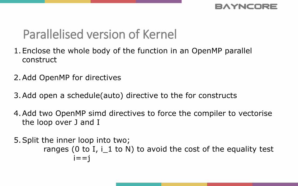
Parallelised version of Kernel1.Enclose the whole body of the function in an OpenMP parallel

construct

2.Add OpenMP for directives

3.Add open a schedule(auto) directive to the for constructs

4.Add two OpenMP simd directives to force the compiler to vectorise the loop over J and I

5.Split the inner loop into two;ranges (0 to I, i_1 to N) to avoid the cost of the equality test

i==j

Modifying the code to offload is easy: specify target and data. This forces the compiler to create two versions of code; processor and co-processor

#pragma omp target datamap (tofrom: x[0:n], y[0:n], z[0:n])map (to: vx[0:n], vy[0:n], vz[0:n], m[0:n] )

For (int it=0; it<100; it++){

Newton(n, 0.01);}

Inadequate Load Balancing

Results indicate speed up as we increase the number of threads (2 processors – left, coprocessor – right).

Offloading decreases the computation time for both double and single precision calculations (2 host processors, and one coprocessor)

Both the host and the Offload device are working at capacity – they can now share the workload.

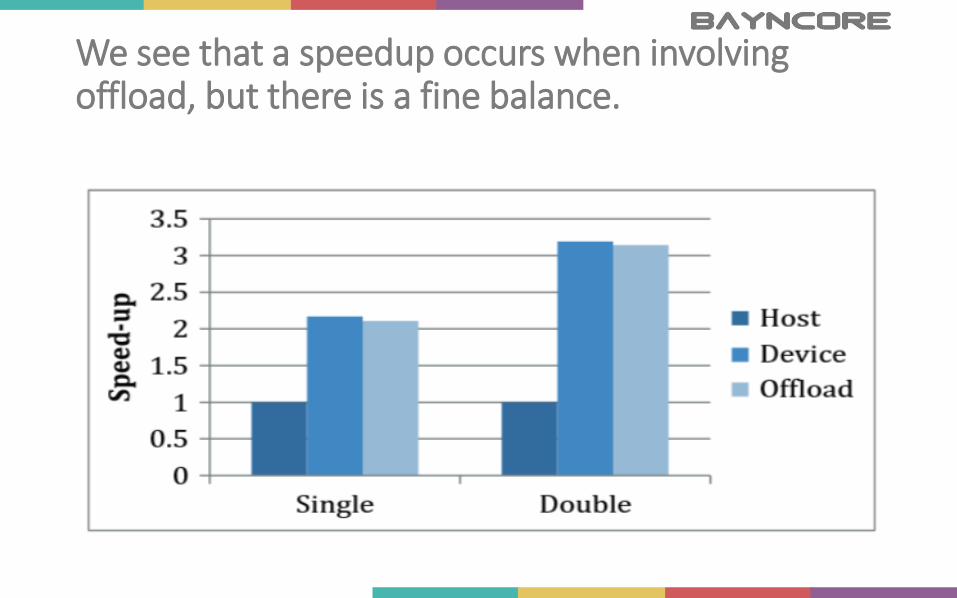
We see that a speedup occurs when involving offload, but there is a fine balance.

Well used processors – workloads tailored to match individual capacities.

• This requires configuring the system to run parallel on the host and the offload device:omp_set_nested(true)

• We need to create 2 threads to allow the host and the device part to work together#pragma omp parallel num_threads(2)

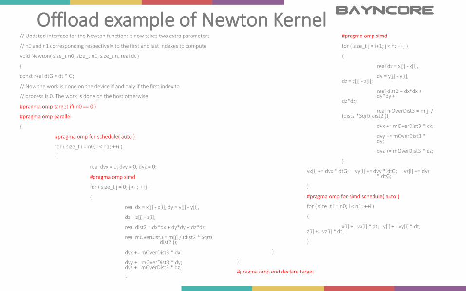
Offload example of Newton Kernel// Updated interface for the Newton function: it now takes two extra parameters

// n0 and n1 corresponding respectively to the first and last indexes to compute

void Newton( size_t n0, size_t n1, size_t n, real dt )

{

const real dtG = dt * G;

// Now the work is done on the device if and only if the first index to

// process is 0. The work is done on the host otherwise

#pragma omp target if( n0 == 0 )

#pragma omp parallel

{

#pragma omp for schedule( auto )

for ( size_t i = n0; i < n1; ++i )

{

real dvx = 0, dvy = 0, dvz = 0;

#pragma omp simd

for ( size_t j = 0; j < i; ++j )

{

real dx = x[j] - x[i], dy = y[j] - y[i],

dz = z[j] - z[i];

real dist2 = dx*dx + dy*dy + dz*dz;

real mOverDist3 = m[j] / (dist2 * Sqrt( dist2 ));

dvx += mOverDist3 * dx;

dvy += mOverDist3 * dy; dvz += mOverDist3 * dz;

}

#pragma omp simd

for ( size_t j = i+1; j < n; ++j )

{

real dx = x[j] - x[i],

dy = y[j] - y[i], dz = z[j] - z[i];

real dist2 = dx*dx + dy*dy +

dz*dz;

real mOverDist3 = m[j] / (dist2 *Sqrt( dist2 ));

dvx += mOverDist3 * dx;

dvy += mOverDist3 * dy;

dvz += mOverDist3 * dz;

}

vx[i] += dvx * dtG; vy[i] += dvy * dtG; vz[i] += dvz* dtG;

}

#pragma omp for simd schedule( auto )

for ( size_t i = n0; i < n1; ++i )

{

x[i] += vx[i] * dt; y[i] += vy[i] * dt; z[i] += vz[i] * dt;

}

}

}

#pragma omp end declare target

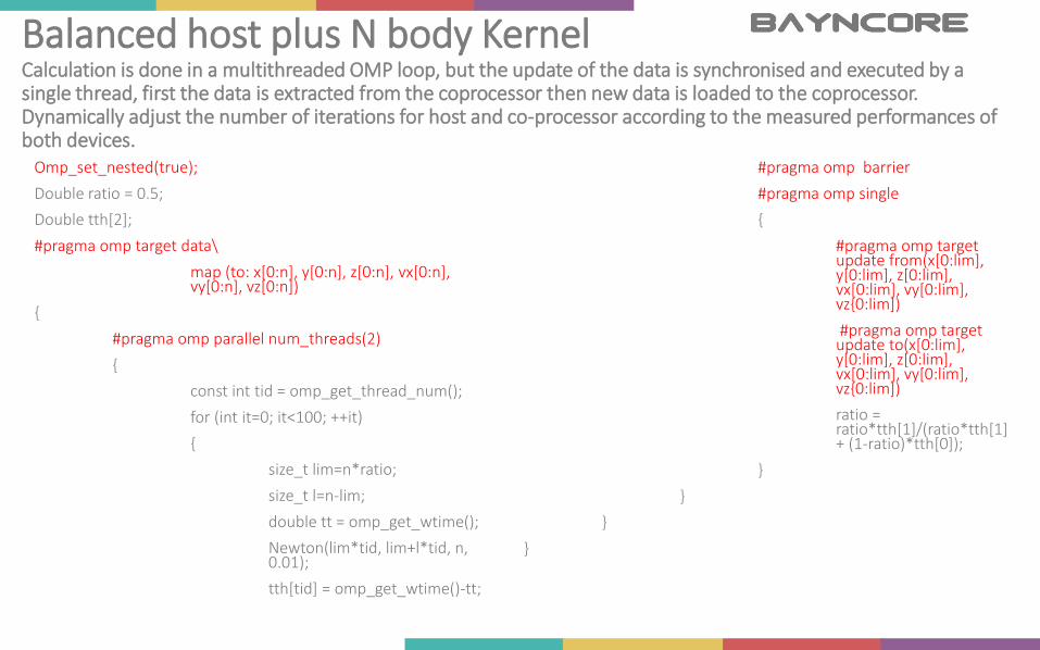
Balanced host plus N body KernelCalculation is done in a multithreaded OMP loop, but the update of the data is synchronised and executed by a single thread, first the data is extracted from the coprocessor then new data is loaded to the coprocessor. Dynamically adjust the number of iterations for host and co-processor according to the measured performances of both devices.

Omp_set_nested(true);

Double ratio = 0.5;

Double tth[2];

#pragma omp target data\

map (to: x[0:n], y[0:n], z[0:n], vx[0:n], vy[0:n], vz[0:n])

{

#pragma omp parallel num_threads(2)

{

const int tid = omp_get_thread_num();

for (int it=0; it<100; ++it)

{

size_t lim=n*ratio;

size_t l=n-lim;

double tt = omp_get_wtime();

Newton(lim*tid, lim+l*tid, n, 0.01);

tth[tid] = omp_get_wtime()-tt;

#pragma omp barrier

#pragma omp single

{

#pragma omp target update from(x[0:lim], y[0:lim], z[0:lim], vx[0:lim], vy[0:lim], vz{0:lim])

#pragma omp target update to(x[0:lim], y[0:lim], z[0:lim], vx[0:lim], vy[0:lim], vz{0:lim])

ratio = ratio*tth[1]/(ratio*tth[1] + (1-ratio)*tth[0]);

}

}

}

}

We see predictably there is a speed up in the calculation as we include the Xeon-Phi platform. Greater for double precision calculations

After a short warm up phase the proportion of the work offloaded to the coprocessors and processor stabilises.

Productive Offloading to multiple devices

Test for number of devices, map data accordingly, set up a parallel for loop for calculation

Const int dev = omp_get_num_devices();#pragma omp parallel num_threads(dev+1){

{ int tid = omp_get_thread_num();#pragma omp target data device(tid)

map(to:x[0:n], y[0:n], z[0:n], m[0:n], vx[0:n], vy[0:n], vz[0:n])

for(int it=0; it<100; ++it){

• Omp_get_num_devices returns the number of devices possible to OFFLOAD

• Device(int) specifies a particular device to be OFFLOADED to• The trick is to use one thread per device to do the work

Load Balancing between multiple devices –mathematical analysisOverall aim is to prevent all of the threads in the system from being idle.

So need to alter the amount of work given to each of the system components to ensure that each portion of the work is concluded at the same time. This is done using the following formula.

𝑟′ =𝑡ℎ𝑟

𝑡ℎ𝑟 + 𝑡𝑏𝑟𝑟′ 𝑇ℎ𝑖𝑠 𝑖𝑠 𝑡ℎ𝑒 𝑛𝑒𝑤 𝑟𝑎𝑡𝑖𝑜 𝑡𝑜 𝑏𝑒 𝑢𝑠𝑒𝑑 𝑖𝑛 𝑡ℎ𝑒 𝑛𝑒𝑥𝑡 𝑖𝑡𝑒𝑟𝑎𝑡𝑖𝑜𝑛𝑟 𝑇ℎ𝑖𝑠 𝑖𝑠 𝑡ℎ𝑒 𝑟𝑎𝑡𝑖𝑜 𝑜𝑓 𝑡ℎ𝑒 𝑤𝑜𝑟𝑘 𝑑𝑜𝑛𝑒 𝑎𝑡 𝑡ℎ𝑒 𝑑𝑒𝑣𝑖𝑐𝑒 𝑜𝑛 𝑡ℎ𝑒 𝑝𝑟𝑒𝑣𝑖𝑜𝑢𝑠 𝑖𝑡𝑒𝑟𝑎𝑡𝑖𝑜𝑛.

𝑡ℎ 𝑇𝑖𝑚𝑒 𝑠𝑝𝑒𝑛𝑡 𝑜𝑛 𝑡ℎ𝑒 𝑐𝑜𝑚𝑝𝑢𝑡𝑎𝑡𝑖𝑜𝑛 𝑜𝑛 𝑡ℎ𝑒 ℎ𝑜𝑠𝑡

𝑡𝑏 𝑇𝑖𝑚𝑒 𝑠𝑝𝑒𝑛𝑡 𝑜𝑛 𝑐𝑜𝑚𝑝𝑢𝑡𝑎𝑡𝑖𝑜𝑛 𝑜𝑛 𝑡ℎ𝑒 𝑑𝑒𝑣𝑖𝑐𝑒

Normalisation condition

𝑖=0

𝑑𝑒𝑣

𝑟𝑖′ = 1

• Measure time• Calculate proportions• Divide work accordingly

Load balancing between multiple devices

Assume each compute device runs at its own speed.

We can compute the starting indices for each off-load device (derivation in Parallel Pears book)

Void computeDisplacements (siz_t *displ, const double *tth, int dev){

double sumLengthOverT = 0;size_t length[dev+1];for (int i=0; i<dev+1; ++i){

length[i] =disp[i+1] –disp[i];for(int i=0; i<dev+1; ++i){

sumLengthOverT += length[i]/tth[i];for(int i=0; i<dev; ++i){

displ[i+1] = displ[i] + round((displ[dev+1]*length[i])/(tth[i]*sumLengthOverT));

}

The retrieval of the results from the offload device is done within a critical section. Whereas the loading of the computation to the offload devices is done in parallel.

For int it=0; it<100; ++it)

{

size_t s = displ[tid], l = disp[tid+1] – disp[tid];

double tt = omp_get_wtime();

Newton(n, s, l, 0.01, tid,dev);

tth[tid] = omp_get_wtime() –tt;

#pragma omp critical

{

#pragma omp target update device (tid)

{

if(tid<dev)

from(x[s:l], y[s:l], z[s:l], vx[s:l],vy[s:l],vz[s:l])

}

#pragma omp barrier

#pragma omp target update device(tid)

if(tid<dev)

to( x[0:s], y[0:s], z[0:s], vx[0:s], vy[0:s], vz[0:s])

size_t s1 = s+1, l1=n-s-l;

#pragma omp target update device (tid)

if(tid<dev)

to (x[s1:l1], y[s1,:l1], z{s1, l1], vx[s1:l1], vy[s1,:l1], vz{s1, l1])

#pragma omp single

computedisplacements (displ, tth, dev);

}

Predictably the more hardware we use the greater the speed up

Evolution of the ratios of the workloads with time

Thankyou

31