Embed Size (px)
Citation preview
박 사 학 위 논 문
Ph.D. Dissertation
변형에너지 변분을 이용한 국부 구조의
실용적인 안정성 평가 방법
A practical method for evaluating stability of local structures
using strain energy variation
2020
오 민 한 (吳 珉 漢 Oh, Min-Han)
한 국 과 학 기 술 원
Korea Advanced Institute of Science and Technology

박 사 학 위 논 문
변형에너지 변분을 이용한 국부 구조의
실용적인 안정성 평가 방법
2020
오 민 한
한 국 과 학 기 술 원
기계항공공학부/기계공학과

변형에너지 변분을 이용한 국부 구조의
실용적인 안정성 평가 방법
오 민 한
위 논문은 한국과학기술원 박사학위논문으로
학위논문 심사위원회의 심사를 통과하였음
2019년 11월 21일
심사위원장 이 필 승 (인 )
심 사 위 원 오 일 권 (인 )
심 사 위 원 김 성 수 (인 )
심 사 위 원 부 승 환 (인 )
심 사 위 원 김 을 년 (인 )

A practical method for evaluating stability of local
structures using strain energy variation
Min-Han Oh
Advisor: Phill-Seung Lee
A dissertation/thesis submitted to the faculty of
Korea Advanced Institute of Science and Technology in
partial fulfillment of the requirements for the degree of
Doctor of Philosophy in Mechanical Engineering
Daejeon, Korea
November 21, 2019
Approved by
Phill-Seung Lee,
Professor of Mechanical Engineering
The study was conducted in accordance with Code of Research Ethics1)
.
1) Declaration of Ethical Conduct in Research: I, as a graduate student of Korea Advanced Institute of Science
and Technology, hereby declare that I have not committed any act that may damage the credibility of my research.
This includes, but is not limited to, falsification, thesis written by someone else, distortion of research findings, and
plagiarism. I confirm that my dissertation contains honest conclusions based on my own careful research under the
guidance of my advisor.

초 록
본 논문에서는 대형 구조물의 국부 안정성을 평가하기 위한 실용적인 방법을 제안한다. 전체
비선형 유한요소(FE) 해석을 통해 계산된 국부 변형 에너지의 2차 변분값을 조사하여 국부
안정성을 평가한다. 이전의 방법들과 달리, 국부 구조와 전체 구조 간의 복잡한 상호 작용을
완벽히 고려할 수 있으며 별도의 국부 FE 해석을 필요로 하지 않는다. FE 모델이 많은 수의
자유도를 가지는 경우, 모델 축소법을 적용하여 계산 효율성을 크게 향상시킬 수 있다. 가장 큰
장점은 제안된 방법이 단순하고 일반적인 구조의 임의 형상 부분에 적용 가능하다는 것이다.
산업계 엔지니어가 적은 노력으로 실용적으로 사용할 수 있다. 몇 가지 수치 예제들을 통해
제안한 평가 방법론의 실효성을 입증하였다.
핵 심 낱 말 국부 안정성, 변형에너지 변분, 비선형 유한요소해석, 모델 축소법, 좌굴
Abstract
In this thesis, we propose a practical method to evaluate the local stability of large size structures. Local stability
is assessed by investigating the second variation of the local strain energy calculated through global nonlinear
finite element (FE) analysis. Unlike previous methods, complicated interactions between local and global
structures are fully considered and the local FE analysis is not necessary. The computational efficiency is greatly
improved by applying the model reduction method to the FE model with a large number of degrees of freedom.
A great advantage is that the proposed method is simple and applicable to arbitrary parts of general structures.
That is, it can be practically used by engineers in industries without much effort. The evaluation methodology is
proposed and its practical effectiveness is demonstrated through several numerical examples.
Keywords Local stability, Strain energy variation, Nonlinear finite element analysis, Model reduction, Buckling
오민한. 변형에너지 변분을 이용한 국부 구조의 실용적인
안정성 평가 방법. 기계공학과. 2020년. 101+ix 쪽. 지도교
수: 이필승. (영문 논문)
Min-Han Oh. A practical method for evaluating stability of local
structures using strain energy variation. Department of Mechanical
Engineering. 2020. 101+ix pages. Advisor: Phill-Seung Lee. (Text in
English)


i
Contents
Contents ............................................................................................................................................................... i
List of Tables ..................................................................................................................................................... ii
List of Figures ................................................................................................................................................... iii
Nomenclature .................................................................................................................................................... ix
Chapter 1 Introduction ........................................................................................................................................ 1
Chapter 2 Structural stability .............................................................................................................................. 7
2.1 Variation criterion for stable state ..................................................................................................... 7
2.2 Incremental strain energy criterion using nonlinear FE method ...................................................... 12
Chapter 3 Evaluation of local stability ............................................................................................................. 14
3.1 Evaluation through the local FE analysis ........................................................................................ 14
3.2 Direct evaluation through the global FE analysis ............................................................................ 16
Chapter 4 Numerical examples ......................................................................................................................... 20
4.1 Stiffened rectangular plate structure in ship-shaped structure ......................................................... 20
4.2 Cylindrical shell structure with radial bulkheads ............................................................................ 31
4.3 Horizontally stiffened cylindrical structure with radial bulkheads .................................................. 38
4.4 Bracket girder in the column-pontoon connection structure of tension leg platform ...................... 44
Chapter 5 Computational efficiency ................................................................................................................. 54
5.1 Reliability and applicability of model reduction method ................................................................ 54
5.2 Comparisons with reduced domain analyses ................................................................................... 71
5.2.1 Horizontally stiffened cylindrical structure with radial bulkheads ...................................... 71
5.2.2 Bracket girder in the column-pontoon connection structure of tension leg platform ........... 82
5.3 Computational efficiency improvement .......................................................................................... 92
Chapter 6 Concluding Remarks ........................................................................................................................ 94
Bibliography ..................................................................................................................................................... 96
Acknowledgments in Korean ......................................................................................................................... 101

ii
List of Tables
Table 1. Local safety factors for a stiffened rectangular plate structure in ship-shaped structure .................... 22
Table 2. Local safety factors for a horizontally stiffened cylindrical structure with radial bulkheads ............. 39
Table 3. Stiffness matrix sizes (degrees of freedom) of full and superelement models for FLNG independent
cargo tank ........................................................................................................................................... 61
Table 4. Contact forces and their ratios on tank supports: friction sensitivity check for friction coefficients of
zero and 0.2 ........................................................................................................................................ 65
Table 5. Stiffness matrix sizes (degrees of freedom) of full and superelement models for dry transportation . 68
Table 6. Comparison of maximum contact forces of full and superelement analysis for dry transportation .... 69
Table 7. Comparison of computing time of full and superelement nonlinear analysis for dry transportation .. 69
Table 8. Local safety factors (LSF) of a horizontally stiffened cylindrical structure with radial bulkheads for all
analysis cases ...................................................................................................................................... 79
Table 9. Standard errors of critical local load of reduced domain analyses compared to full domain analysis for a
horizontally stiffened cylindrical structure with radial bulkheads (unit: kN) ..................................... 81
Table 10. Local safety factors (LSF) of a bracket girder in the column-pontoon connection structure of tension leg
platform for analysis cases ................................................................................................................. 89
Table 11. Standard errors of critical local load of reduced domain analyses compared to full domain analysis for a
bracket girder in the column-pontoon connection structure of tension leg platform (unit: kN) ......... 91
Table 12. Computing costs of evaluation domains for a bracket girder in the column-pontoon connection structure
of tension leg platform for all analysis cases ...................................................................................... 92

iii
List of Figures
Fig. 1. Mississippi bridge collapse [1]: (a) bowed gusset plates (June 2003) and (b) overall view after
collapse (August 1, 2007) .................................................................................................................. 1
Fig. 2. Typical local structures in thin-walled ship and offshore structures: stiffened panels, cylindrical shells,
brackets, and opening structures ........................................................................................................ 2
Fig. 3. Illustrations of permanent damages due to local buckling in ship structures [3]: (a) buckling of
stiffened plate, (b) bucking and rupture around plate opening and (c) buckling of web plate ........... 3
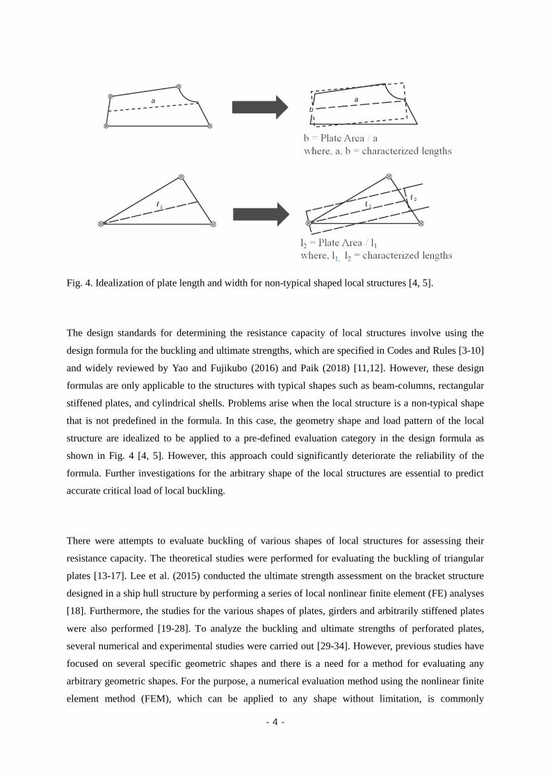
Fig. 4. Idealization of plate length and width for non-typical shaped local structures [4, 5] ........................ 4
Fig. 5. Ball in different gravity field conditions [38]: (a) stable, (b) unstable (neutral equilibrium) and (c)
unstable .............................................................................................................................................. 7
Fig. 6. Schematic models of truss beam structure: (a) a truss alone and (b) a truss with vertical spring ...... 8
Fig. 7. Load - displacement curve for truss beam structure with vertical spring ......................................... 11
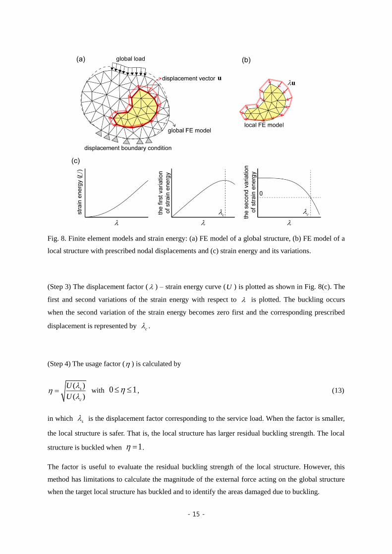
Fig. 8. Finite element models and strain energy: (a) FE model of a global structure, (b) FE model of a local
structure with prescribed nodal displacements and (c) strain energy and its variations ................... 15
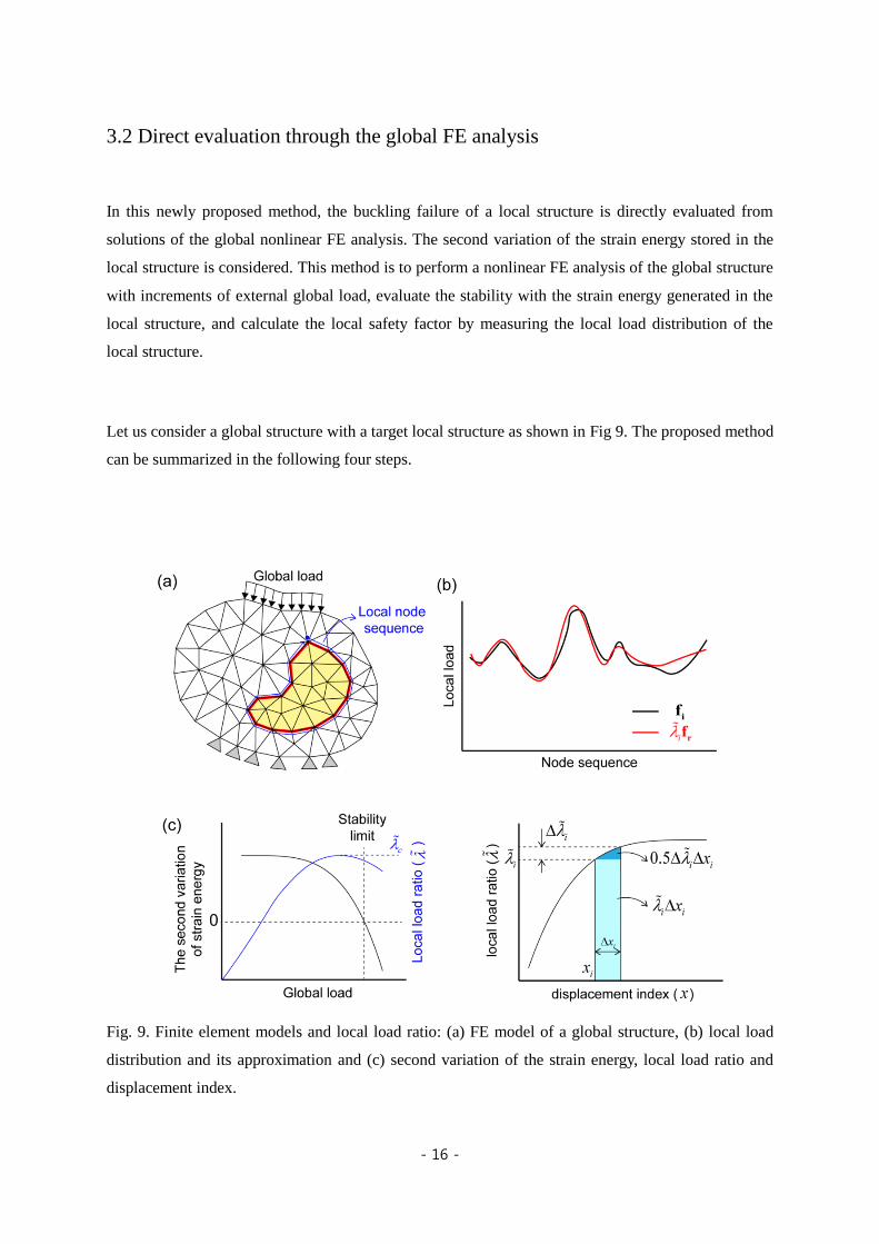
Fig. 9. Finite element models and local load ratio: (a) FE model of a global structure, (b) local load
distribution and its approximation and (c) second variation of the strain energy, local load ratio and
displacement index .......................................................................................................................... 16
Fig. 10. Identification of damaged area along to the range of the evaluated area ......................................... 19
Fig. 11. Floating structure and stiffened plate: (a) overview of ship-shaped floating structure under vertical
bending moment and (b) stiffened rectangular local plate structure at the upper sideshell of the
floating structure .............................................................................................................................. 20
Fig. 12. Strain energy composition of force and moment components for local structural domain of a stiffened
rectangular plate structure in ship-shaped structure ......................................................................... 23
Fig. 13. Finite element model, applied global loads and local loads of a stiffened rectangular plate structure in
ship-shaped structure: (a) finite element model, (b) von Mises stress distribution and (c) local loads at
10th analysis step ............................................................................................................................. 24
Fig. 14. The reference local load and calculated local load ratios of a stiffened rectangular plate structure in
ship-shaped structure: (a) reference local load (2nd step), (b) applied and approximated local loads
(10th step), (c) error function of local load (10th step) and (d) calculated local load ratios along the
applied loads .................................................................................................................................... 25
Fig. 15. Stability evaluation with the second variation of the local strain energy, local load ratios and selected
critical local load of a stiffened rectangular plate structure in ship-shaped: (a) second variation of the
local strain energy per unit deformation, (b) local load ratio and displacement index and (c) critical
local load selected from the stability evaluation .............................................................................. 26

iv
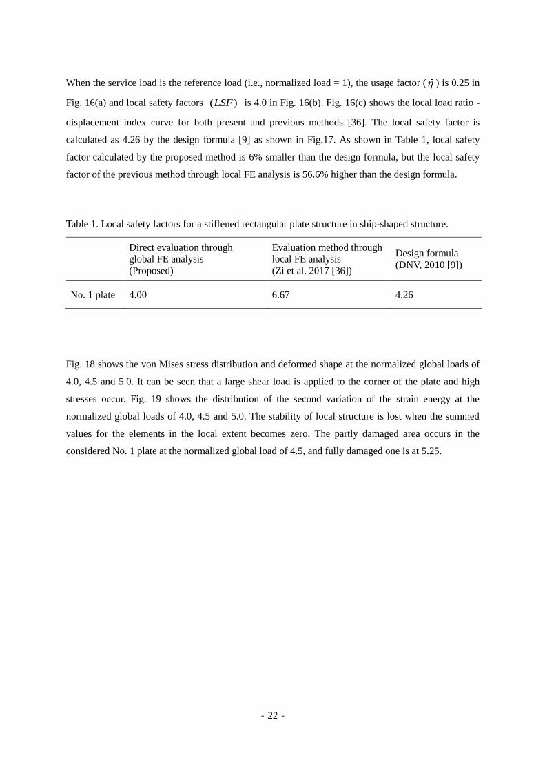
Fig. 16. Calculation of usage factors and local safety factors of a stiffened rectangular plate structure in ship-
shaped structure: (a) usage factors along to service load levels, (b) local safety factors along to service
load levels and (c) comparison of local load ratios with previous study (Zi et al. 2017) ................. 27
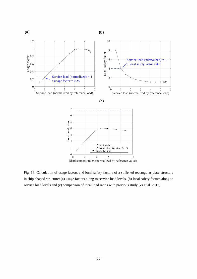
Fig. 17. Calculation of the safety of the Plate No. 1 in a stiffened rectangular plate structure in ship-shaped
structure by the design formula of DNV-RP-C201 [9] .................................................................... 28
Fig. 18. von Mises stress plots (unit: MPa) and deformed shapes (30-time scale) of the Plate No. 1 in a
stiffened rectangular plate structure in ship-shaped structure. The normalized global loads are (a) 4.0,
(b) 4.5 and (c) 5.0 ............................................................................................................................ 29
Fig. 19. Second variation of the strain energy plots (unit: Nmm) and damaged areas of the Plate No. 1 in a
stiffened rectangular plate structure in ship-shaped structure. The normalized global loads are (a) 4.0,
(b) 4.5 and (c) 5.0 ............................................................................................................................ 30
Fig. 20. Monocolumn FPSO for North Sea field: (a) overview of monocolumn FPSO [40], (b) inner view of
cylindrical shell and radial bulkhead in a simplified model, and (c) inner view of cylindrical shell and
radial bulkhead with horizontal stringer in a simplified model ....................................................... 31
Fig. 21. Simplified structural strip model of a cylindrical shell structure with radial bulkheads in monocolumn
FPSO ................................................................................................................................................ 32
Fig. 22. Strain energy of full and local structural domains of a cylindrical shell structure with radial bulkheads
........................................................................................................................................................... 34
Fig. 23. Strain energy composition of force and moment components for local structural domain of a
cylindrical shell structure with radial bulkheads .............................................................................. 34
Fig. 24. Second variation of strain energy in local domain of a cylindrical shell structure with radial bulkheads
........................................................................................................................................................... 35
Fig. 25. Applied global load versus displacement on load points of a cylindrical shell structure with radial
bulkheads ......................................................................................................................................... 35
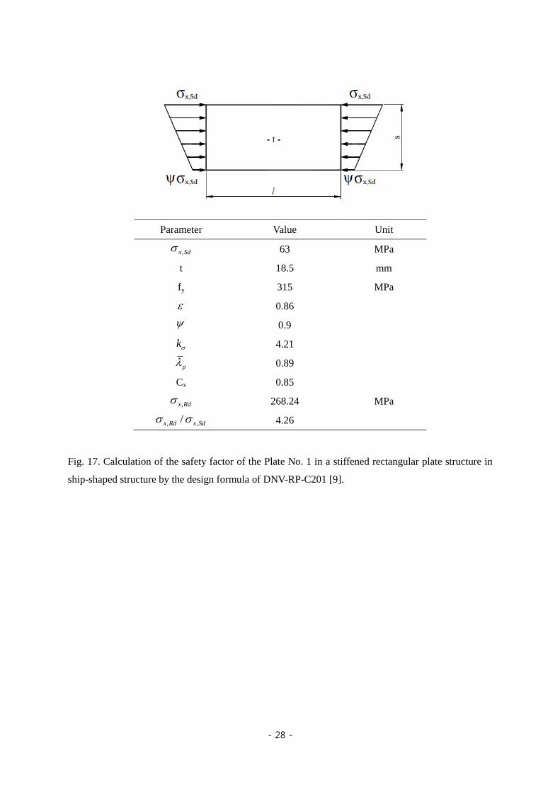
Fig. 26. X–directional deformation contour (unit: mm) and true-scaled deformed shapes of the simplified
structural-strip model in a cylindrical shell structure with radial bulkheads for the evaluation of snap-
through behavior. The applied loads are (a) 0.5 kN, (b) 5 kN, (c) 9.38 kN, and (d) 9.59 kN .......... 36
Fig. 27. Local load ratio - displacement index curve of a cylindrical shell structure with radial bulkheads
......................................................................................................................................................... 37
Fig. 28. Simplified stringer model of a horizontally stiffened cylindrical structure with radial bulkheads in
monocolumn FPSO .......................................................................................................................... 38
Fig. 29. Strain energy composition of force and moment components for local structural domain of a
horizontally stiffened cylindrical structure with radial bulkheads ................................................... 40
Fig. 30. Second variation of strain energy in local domain of a horizontally stiffened cylindrical structure with
radial bulkheads ............................................................................................................................... 40
v
Fig. 31. Elastic and plastic deformations (five-time scale) of a stiffened cylindrical shell structure with radial
bulkheads. The applied loads are (a) 1 MPa, (b) 7 MPa, (c) 10.59 MPa, and (d) 10.76 MPa. The red
color indicates that the element has reached the material yield stress ............................................. 41
Fig. 32. Local load ratio - displacement index curve of a horizontally stiffened cylindrical structure with radial
bulkheads ......................................................................................................................................... 41
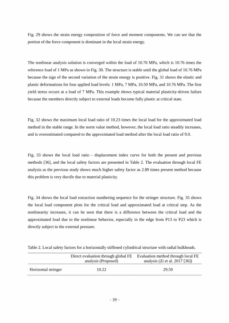
Fig. 33. Local load ratios of a stiffened cylindrical shell structure with radial bulkheads with previous study
(Zi et al. 2017) ................................................................................................................................. 42
Fig. 34. Local load extraction numbering sequence for horizontal stringers structure of a horizontally stiffened
cylindrical structure with radial bulkheads ...................................................................................... 42
Fig. 35. Local load component plots (unit: MPa) for the critical load and approximated load at critical step of
a horizontally stiffened cylindrical structure with radial bulkheads ................................................ 43
Fig. 36. TLP installed in West Africa field: (a) Photo of TLP [41], (b) schematic of TLP hull with column and
pontoon structures, and (c) plan view of the bracket girder between column and pontoons ........... 44
Fig. 37. Finite element model of a column-pontoon connection structure of tension leg platform ............... 45
Fig. 38. Finite element model of a bracket girder of interest in the column-pontoon connection structure of
tension leg platform ......................................................................................................................... 45
Fig. 39. Finite element model and applied loads of a bracket girder in the column-pontoon connection
structure of tension leg platform ...................................................................................................... 46
Fig. 40. Strain energy composition of force and moment components for local structural domain of a bracket
girder in the column-pontoon connection structure of tension leg platform .................................... 48
Fig. 41. Second variation of strain energy in local domain of a bracket girder in the column-pontoon
connection structure of tension leg platform .................................................................................... 48
Fig. 42. Elastic and plastic deformations (three-time scale) of a bracket girder in the column-pontoon
connection structure of tension leg platform. Applied normalized global loads are (a) 1.0, (b) 2.0, (c)
3.1, (d) 3.5, (e) 3.8, and (f) 4.0. The red color indicates that the element has reached the material yield
stress .................................................................................................................................................. 49
Fig. 43. Deformation of a bracket girder in the column-pontoon connection structure of tension leg platform:
(a) vertical (z-) direction displacement contour (unit: mm) at critical state and (b) vertical (z-)
direction displacement on point A under the various applied loads ................................................. 50
Fig. 44. Local load extraction numbering sequence of a bracket girder in the column-pontoon connection
structure of tension leg platform ...................................................................................................... 51
Fig. 45. Local load component plots for the critical load and approximated load at critical step of a bracket
girder in the column-pontoon connection structure of tension leg platform .................................... 52
Fig. 46. Local load - displacement index curve of a bracket girder in the column-pontoon connection structure
of tension leg platform ..................................................................................................................... 53
Fig. 47. Schematic of the model reduction method with static condensation for local structural stability
evaluation ......................................................................................................................................... 55

vi
Fig. 48. Simple FE model for nonlinear superelement analysis verification ............................................... 57
Fig. 49. Notation of gap elements: ant-pitch (AP) and vertical (VT) elements ............................................. 57
Fig. 50. Normalized contact and friction force comparison between full FE model and condensed FE model
using the proposed superelement method (static and slip friction coefficient = 0.2, convergence
criteria: EPSP = 1E−3 and EPSW = 1E−5); (a) contact force, (b) friction(i) force, and (c) friction(ii)
force ................................................................................................................................................. 58
Fig. 51. Example of independent cargo tank supports [47]: (a) the mid ship section, (b) the vertical support
model and (c) the anti-roll and anti-pitch support models ............................................................... 60
Fig. 52. Hydrodynamic and internal tank pressure RAO (LNG tank fully-loaded condition, quartering sea, ω=
0.398) ............................................................................................................................................... 61
Fig. 53. Considered anti-roll support location in a starboard side tank ......................................................... 63
Fig. 54. Considered anti-pitch and vertical support locations in a starboard side tank ................................. 63
Fig. 55. Maximum vertical contact forces on vertical support (static and slip friction coefficient = 0.2,
convergence criteria: EPSP = 1E−3 and EPSW = 1E−5) ................................................................ 64
Fig. 56. Maximum transverse contact forces on lower anti-roll support (static and slip friction coefficient =
0.2, convergence criteria: EPSP = 1E−3 and EPSW = 1E−5) ......................................................... 64
Fig. 57. Maximum transverse contact forces on upper anti-roll support (static and slip friction coefficient =
0.2, convergence criteria: EPSP = 1E−3 and EPSW = 1E−5) ......................................................... 64
Fig. 58. Maximum longitudinal contact forces on anti-pitch support (static and slip friction coefficient = 0.2,
Convergence criteria: EPSP = 1E−3 and EPSW = 1E−5) ............................................................... 64
Fig. 59. Overall FE model of dry transportation ........................................................................................... 67
Fig. 60. Detailed view of sea-fastening stopper and gap elements between cargo and transportation barge: (a)
plated structure and (b) vertical columns ......................................................................................... 67
Fig. 61. Deformed shape of dry transportation model for load case 2 .......................................................... 68
Fig. 62. Nonlinear analysis domain of a stringer of a horizontally stiffened cylindrical structure with radial
bulkheads for model reduction and prescribed displacement analysis ............................................. 72
Fig. 63. Nonlinear analysis domain of the extended stringer of a horizontally stiffened cylindrical structure
with radial bulkheads for extended model reduction ....................................................................... 72
Fig. 64. Second variation of strain energy in local domain of a horizontally stiffened cylindrical structure with
radial bulkheads for model reduction case ....................................................................................... 74
Fig. 65. Second variation of strain energy in local domain of a horizontally stiffened cylindrical structure with
radial bulkheads for extended model reduction case ....................................................................... 74
Fig. 66. Second variation of strain energy in local domain of a horizontally stiffened cylindrical structure with
radial bulkheads for prescribed displacement case .......................................................................... 75
Fig. 67. Local load ratio – displacement index curve of a horizontally stiffened cylindrical structure with
radial bulkheads for all analysis cases ............................................................................................. 75
vii
Fig. 68. Local load component plots for the critical load and approximated load at critical step of a
horizontally stiffened cylindrical structure with radial bulkheads for model reduction case ........... 76
Fig. 69. Local load component plots for the critical load and approximated load at critical step of a
horizontally stiffened cylindrical structure with radial bulkheads for extended model reduction
case .................................................................................................................................................. 77
Fig. 70. Local load component plots for the critical load and approximated load at critical step of a
horizontally stiffened cylindrical structure with radial bulkheads for prescribed displacement
case .................................................................................................................................................. 78
Fig. 71. Local safety factors of a horizontally stiffened cylindrical structure with radial bulkheads ............ 79
Fig. 72. Local load component plots for the critical load and approximated load at critical step of a
horizontally stiffened cylindrical structure with radial bulkheads for all analysis cases ................. 80
Fig. 73. Standard errors of critical local load of reduced domain analyses compared to critical full domain
analysis of a horizontally stiffened cylindrical structure with radial bulkheads. Standard error is
defined as ( ) ( )f f f fi i ref i i ref , where fi is i-th local load vector and ( )fi ref is i-th
local load vector in full domain analysis as the reference value ...................................................... 81
Fig. 74. Nonlinear analysis domain of a bracket girder in the column-pontoon connection structure of tension
leg platform for model reduction and prescribed displacement ....................................................... 83
Fig. 75. Nonlinear analysis domain of the extended bracket girder structure in the column-pontoon connection
structure of tension leg platform for extended model reduction ...................................................... 83
Fig. 76. Second variation of strain energy in local domain of a bracket girder in the column-pontoon
connection structure of tension leg platform for model reduction case ........................................... 84
Fig. 77. Second variation of strain energy in local domain of a bracket girder in the column-pontoon
connection structure of tension leg platform for extended model reduction case ............................ 84
Fig. 78. Second variation of strain energy in local domain of a bracket girder in the column-pontoon
connection structure of tension leg platform for prescribed displacement case ............................... 85
Fig. 79. Local load ratio – displacement index curve of a bracket girder in the column-pontoon connection
structure of tension leg platform for all analysis cases .................................................................... 85
Fig. 80. Local load component plots for the critical load and approximated load at critical step of a bracket
girder in the column-pontoon connection structure of tension leg platform for model reduction
case .................................................................................................................................................. 86
Fig. 81. Local load component plots for the critical load and approximated load at critical step of a bracket
girder in the column-pontoon connection structure of tension leg platform for extended model
reduction case .................................................................................................................................. 87
Fig. 82. Local load component plots for the critical load and approximated load at critical step of a bracket
girder in the column-pontoon connection structure of tension leg platform for prescribed displacement
case .................................................................................................................................................. 88
viii
Fig. 83. Maximum local load ratios of a bracket girder in the column-pontoon connection structure of tension
leg platform for all analysis cases .................................................................................................... 89
Fig. 84. Local load component plots for the critical load and approximated load at critical step of a bracket
girder in the column-pontoon connection structure of tension leg platform for all analysis cases .. 90
Fig. 85. Standard errors of critical local load for reduced domain analyses compared to critical full domain
analysis of a bracket girder in the column-pontoon connection structure of tension leg platform.
Standard error is defined as ( ) ( )f f f fi i ref i i ref , where fi is i-th local load vector and
( )fi ref is i-th local load vector in full domain analysis as the reference value ................................ 91
Fig. 86. Total computing time comparison for a bracket girder in the column-pontoon connection structure of
tension leg platform for all analysis cases ....................................................................................... 93

ix
Nomenclature
potential energy
U strain energy
W work of load
iq
i-th general displacement variable
E Young’s modulus of truss beam
strain of truss beam
L length of truss beam
A area of truss beam
initial angle of truss beam
applied angle of truss beam
P applied load of truss beam
q applied vertical displacement of truss beam
fi i-th step applied load vector
fr reference load vector
u
displacement vector
displacement factor
,s c
displacement factor at service load and critical load
usage factor
usage factor for proposed method
local load ratio by approximated load method
,s c
local load ratio by approximated load method at service load and critical load
local load ratio by norm value method
i i-th step error function
ix
i-th step displacement index
EPSP error tolerance for load (P) criterion
EPSW error tolerance for work (W) criterion
LSF local safety factor

- 1 -
Chapter 1. Introduction
Steels are commonly used in civil, ship and offshore structures. Since the steels are characterized by
high strength and high toughness, and tensile and compressive strengths are almost the same, steel
structures can be designed to be thin-walled. However, this characteristic is likely to cause local
structural failures mainly due to buckling. The structural instability due to buckling is a very
dangerous phenomenon in terms of structural safety.
In the past, a Mississippi bridge collapse occurred in 2007 as shown in Fig. 1 [1]. The primary cause
of the collapse was due to the poor structural stability (buckling) evaluation of the small gusset plate,
which did not account for the increased load. The concrete had been added to the road surface over
the years, and the extraordinary weight of construction equipment and material rested on the bridge
just above its weakest point at the time of the collapse. This unexpected load increase caused lateral
buckling of the load-carrying local gusset structure, followed by a sudden collapse of the entire
structure. It is recorded as a major disaster that caused the whole structure collapse due to poor
evaluation of the structural stability of the local structure.
(a) (b)
Fig. 1. Mississippi bridge collapse [1]: (a) bowed gusset plates (June 2003) and (b) overall view after
collapse (August 1, 2007).

- 2 -
Fig. 2. Typical local structures in thin-walled ship and offshore structures: stiffened panels, cylindrical
shells, brackets, and opening structures.
The buckling refers to the loss of stability of a component structure. The buckling strength is to be
checked on the local strength level [2]. Fig. 2 shows various local parts of structures (or local
structures), for which local buckling is considered in structural design. Fig. 3 illustrates permanent
damages due to the local buckling [3]. When a local buckling happens, excessive local deformation
occurs and the entire load resistance can be significantly reduced. The progressive local buckling
would lead to a global failure of the structure. To maintain robust structural systems with desired
capacity, it is important to ensure that local structures still contribute to the entire resistance. If
necessary, local reinforcement should be applied. For such purposes, the accurate evaluation of the
local stability is essential. However, local and global structures are complexly connected. This fact
makes the stability evaluation very difficult, especially, for structures with complicated geometry.

- 3 -
(a)
(b)
(c)
Fig. 3. Illustrations of permanent damages due to local buckling in ship structures [3]: (a) buckling of
stiffened plate, (b) bucking and rupture around plate opening and (c) buckling of web plate.
- 4 -
Fig. 4. Idealization of plate length and width for non-typical shaped local structures [4, 5].
The design standards for determining the resistance capacity of local structures involve using the
design formula for the buckling and ultimate strengths, which are specified in Codes and Rules [3-10]
and widely reviewed by Yao and Fujikubo (2016) and Paik (2018) [11,12]. However, these design
formulas are only applicable to the structures with typical shapes such as beam-columns, rectangular
stiffened plates, and cylindrical shells. Problems arise when the local structure is a non-typical shape
that is not predefined in the formula. In this case, the geometry shape and load pattern of the local
structure are idealized to be applied to a pre-defined evaluation category in the design formula as
shown in Fig. 4 [4, 5]. However, this approach could significantly deteriorate the reliability of the
formula. Further investigations for the arbitrary shape of the local structures are essential to predict
accurate critical load of local buckling.
There were attempts to evaluate buckling of various shapes of local structures for assessing their
resistance capacity. The theoretical studies were performed for evaluating the buckling of triangular
plates [13-17]. Lee et al. (2015) conducted the ultimate strength assessment on the bracket structure
designed in a ship hull structure by performing a series of local nonlinear finite element (FE) analyses
[18]. Furthermore, the studies for the various shapes of plates, girders and arbitrarily stiffened plates
were also performed [19-28]. To analyze the buckling and ultimate strengths of perforated plates,
several numerical and experimental studies were carried out [29-34]. However, previous studies have
focused on several specific geometric shapes and there is a need for a method for evaluating any
arbitrary geometric shapes. For the purpose, a numerical evaluation method using the nonlinear finite
element method (FEM), which can be applied to any shape without limitation, is commonly
- 5 -
recommended [35].
The basic difficulty is that the resistance capacity of local structures is hard to distinguish because the
local structures are included in a global structure with complicated couplings. That is, the local
behavior is not independent from the global one. To overcome these limitations, Zi et al. (2017)
separated the local and global behaviors and employed nonlinear finite element analysis for a local
bracket girder structure [36]. The reference displacement vector on the boundary of the local bracket
girder was extracted from the linear global finite element analysis, and then the local finite element
analysis was performed linearly-incrementing the prescribed reference displacement. The method was
successful for the local stability evaluation of an arbitrarily shaped bracket girder in an offshore
structure. However, the coupling between local and global structures was not considered.
In this thesis, an adoptable evaluation method of local stability of structures by using nonlinear finite
element analysis is proposed. Of course, the coupling between local and global structures is fully
considered. The energy criterion of the local structure is investigated to evaluate the structural
stability as the extension of the energy method developed by Zi et al. [36]. The accuracy and
efficiency of the evaluation procedure are improved in the practical structural design aspect. For this,
we define the local load of the considered local structure and the representative local load ratio for the
quantitative safety factor assessment. In this step, the local load distribution is approximately fitted to
the reference value with a scalar factor. A displacement index is introduced to show the physical
quantities representing the equivalent displacement level. For a large number of degrees of freedom
problem, the analysis time can be significantly reduced by applying the model reduction method. The
proposed method is simple and applicable to arbitrary parts of general global structures. We illustrate
the usefulness of the proposed method through four examples: a stiffened rectangular plate structure
in a ship-shaped structure, a cylindrical shell structure with radial bulkheads, a horizontally stiffened
cylindrical shell structure with radial bulkheads, and a bracket girder in the column-pontoon
connection structure of tension leg platform. The evaluation procedure uses the nonlinear finite
element analysis by the Newton-Raphson method or the arc-length method [37].

- 6 -
The proposed method can be used for following practical purposes:
We can identify whether the target local structure is buckled. When the target local structure
loses its stability, the corresponding magnitude of the external force acting on the global
structure can be calculated.
We can identify areas where local buckling occurs in the global structure. That is, damaged
areas can be identified.
The residual strength of the damaged areas can be calculated.
When we locally reinforce the damaged areas, the effectiveness of the local reinforcement
can be measured.
We reduce analysis time economically through the model reduction technique for finite
element models with a large number of degrees of freedom.
In Chapter 2 of this paper, the structural stability is reviewed in brief. The proposed evaluation
method is presented in Chapter 3. In Chapter 4, we verify the performance of the proposed method
through several simplified numerical examples and actual large scale problems. Chapter 5 examines
the computational efficiency of the model reduction, and finally, conclusions are presented in Chapter
6.

- 7 -
Chapter 2. Structural stability
In this chapter, we review the definition and formulation for the structural stability and investigate
how incremental nonlinear finite element analysis can be applied to stability evaluation.
2.1 Variation criterion for stable state
Structural stability refers to the phenomenon in which a structure returns to an equilibrium state when
an external displacement disturbance is applied to the structure under this equilibrium state. To
maintain a structurally stable state, the potential energy at the equilibrium state must be the minimum
value [38]. Fig. 5 shows the ball in the gravity field. Fig. 5(a) shows a case where the potential
gravitational energy is minimal and this state is stable.
(a) (b) (c)
Fig. 5. Ball in different gravity field conditions [38]: (a) stable, (b) unstable (neutral equilibrium) and
(c) unstable.
To introduce structural stability, we construct a simple model, derive evaluation equations, and
perform stability assessments. In particular, we choose an example of a sudden snap-buckling as
shown in Fig. 6(a). We see how the overall behavior would change if an additional structure is
attached. Fig. 6(b) illustrates the problem of structural stability of the truss beam with a spring which
simplifies adjacent structures.

- 8 -
(a) (b)
Fig. 6. Schematic models of truss beam structure: (a) a truss alone and (b) a truss with vertical spring.
The potential energy is defined as
U W , (1)
where U is the strain energy and W is the work of loads.
According to the law of conservation of energy, the equilibrium state of a structure with respect to a
given change in load or displacement means that the change in potential energy is zero as below:
0U W . (2)
That is, in the equilibrium state, the value of is always a constant. If the is continuous
derivatives, the function may be expanded into a Taylor series with second-order variations about
the equilibrium state:
2
1 1 1,..., ,....,n n nq q q q q q (3)
with 1
n
i
i i
and
22
1 1
1
2
n n
i j
i j i j
q qq q
,
in which iq is small variations in the i-th generalized displacements from the equilibrium state at
constant load, and and 2 are the first and second variations of the potential energy,
respectively.

- 9 -
The conditions of equilibrium are
0 for any iq , (4a)
or 0iq
for each i . (4b)
According to the Lagrange-Dirichlet theorem, the equilibrium state is stable for those values of the
constant load for which
2 0 for any iq , jq . (5)
To obtain the variation criterion for satisfying the stable state for the snap-through problem in Fig.
7(a), we find the potential energy:
2
21 cos2 1
2 cos cos
EALU W E dV Pq Pq
(6)
with 1tan tan
q
L
,
where E , , L , and A are the Young’s modulus, strain, length and section area of the truss
member, respectively, and is the initial angle, is the applied angle, P is the applied load,
and q is the applied vertical displacement.
To decide the question of stability of equilibrium states, we need to calculate the second-order
derivative of :
2
3 3 1
2
2 2cos cos cos cos tan tan
EA EA q
q L L L
. (7)
The truss is stable if this expression is positive as
2
20
q
.

- 10 -
This yields the condition that
3cos cos 0 , or (8a)
3 1cos cos tan tan 0q
L
. (8b)
We examine how snap-through phenomena change if we add additional stiffness in addition to the
structure in which snap-through occurs. Fig. 6(b) shows the case where the grounded spring is added
to the load application point in Fig. 6(a). Considering the case of a spring in the direction of load, we
find the potential energy with a vertical stiffness:
2
2 2 21 1 cos 12 1
2 2 cos cos 2
EALE dV Kq Pq Kq Pq
, (9)
where K is additional grounded spring stiffness.
To decide the question of stability of equilibrium states, we need to calculate the second-order
derivative of .
2
3 3 1
2
2 2cos cos cos cos tan tan
EA EA qK K
q L L L
. (10)
The truss is stable if this expression is positive as
2
20
q
.
This yields the condition that
32cos cos 0
EAK
L , or (11a)
3 12cos cos tan tan 0
EA qK
L L
. (11b)

- 11 -
Fig. 7. Load - displacement curve for truss beam structure with vertical spring.
Whether the entire structure may be stable is depending on the spring stiffness value attached to the
truss structure as shown in Fig. 7. The global load ( )G iP q is applied when the displacement is at iq
and the local load ( )L iP q of a part of the local structure works. It can be seen that the global load
and displacement are nonlinear relationships. The truss structure itself with zero spring stiffness
unstably behaves like the snap buckling after the load reaches the critical load ( )L cP q as the curve
(a). However, the entire structure may be the stable state when the adjacent structure is relatively stiff
as the curve (b). In other words, it means that even if the entire structure is stable, the local structure
itself may already be in a state of losing its stability. The instability of the local structure makes it not
to have the resistance to the external load. If additional external loads are applied, local deformation
may increase rapidly. For the robust and cost-effective design, the own resistance capacity of the local
structure has to be evaluated reliably and quantitatively. As can be seen in the truss beam model, it
can be precisely identified when the local structure itself loses stability by investigating the second
variation of the potential energy of the local structure.

- 12 -
2.2 Incremental strain energy criterion using nonlinear FE method
When the load has a constant value, the formulation of the second variation of the potential energy
can be simplified to a second variation of the strain energy [36, 38]. For practical purposes, it can be
assumed that there is no load change due to small external displacement disturbances. When this
assumption is applied, we can see that the term of the second-order work regarding the constant load
( P ) is absent in Eqs. (7) and (10). Therefore, when the second variation of the strain energy stored in
structures is from positive to negative, the structure loses stability. This is the energy criterion for
evaluating the stability of structures. The structural resistance can be defined as the maximum load
level within the stable load range obtained from the stability evaluation.
The stability of the structure can be easily evaluated using a nonlinear finite element analysis. We
apply the energy criterion to the target structure using the incremental strain energy value at each
analysis step while incrementing the load or displacement [36, 38]. If the analysis is performed at
sufficiently small intervals, we can precisely find the instant losing stability. In the equilibrium state,
the second variation of the strain energy becomes the second-order term of the incremental external
work according to the law of conservation of energy. Depending on the preference, an evaluation of
the second-order term of the incremental external work can be applied as an energy criterion for the
stability evaluation.
Therefore, if 2 0iW , it becomes a stable state as
0.5 0.5 0f u f ui i i i , (12)
where fi is the load vector and ui
is the displacement vector, and fi and ui
are directly obtained
from results of the nonlinear FE analysis, where the subscript i refers to the i-th analysis step.
This method is effective for evaluating the stability of elastic structures, and it is also applicable to
inelastic structures on the approximation that they are considered as the tangentially equivalent elastic
structures during each small loading step [38]. That is, the structural stability in consideration of the
plasticity of the material can be evaluated.

- 13 -
The method applies initial fabrication imperfections to the target structure in the form of an elastic
buckling mode that easily occurs in the considered load configuration. By applying the initial
imperfections, incremental displacement disturbances corresponding to intended specific load paths
induce the predominant instability for the structure. The method is efficient in terms of calculation
time because it does not consider all possible displacement disturbances and only reflects the
displacement disturbances corresponding to a specific load.

- 14 -
Chapter 3. Evaluation of local stability
In this Chapter, we briefly review the method to evaluate the local stability of structures through
sequential FE analysis of a local structure proposed by Zi et al. (2017) [36]. We then newly propose a
method to directly evaluate the local stability of structures through the global FE analysis.
3.1 Evaluation through the local FE analysis
Recently, Zi et al. proposed an index (usage factor) to measure the safety from the local buckling
failure for the local structures of non-typical geometry. Doing so, linear FE analysis of a global
structure is performed first and nonlinear incremental analysis of a local structure is performed using
the calculated displacement field on the boundary of the local structure included in the global
structure. Then, the critical buckling load can be evaluated by finding the load level which the second
variation of the strain energy of the local structure becomes zero [38].
Considering a target local structure as shown in Fig 8, we here summarize the method proposed by Zi
et al. in the following four steps.
(Step 1) The linear finite element analysis is performed for the global structure, see Fig. 8(a). We then
find the displacement distribution along the interface between the local and global structures (or the
boundary of the local structure). The distribution is represented by a nodal displacement vector u .
(Step 2) We construct the finite element model only for the local structure and apply the prescribed
displacement u with a factor . Note that the displacement distribution is varying depending on
load level in the global structure but we assume that the distribution does not change. Increasing the
displacement factor representing the magnitude of the prescribed displacement, we perform nonlinear
incremental finite element analysis, see Fig. 8(b).
- 15 -
Fig. 8. Finite element models and strain energy: (a) FE model of a global structure, (b) FE model of a
local structure with prescribed nodal displacements and (c) strain energy and its variations.
(Step 3) The displacement factor ( ) – strain energy curve (U ) is plotted as shown in Fig. 8(c). The
first and second variations of the strain energy with respect to is plotted. The buckling occurs
when the second variation of the strain energy becomes zero first and the corresponding prescribed
displacement is represented by c .
(Step 4) The usage factor ( ) is calculated by
( )
( )
s
c
U
U
with 0 1 , (13)
in which s is the displacement factor corresponding to the service load. When the factor is smaller,
the local structure is safer. That is, the local structure has larger residual buckling strength. The local
structure is buckled when 1 .
The factor is useful to evaluate the residual buckling strength of the local structure. However, this
method has limitations to calculate the magnitude of the external force acting on the global structure
when the target local structure has buckled and to identify the areas damaged due to buckling.
- 16 -
3.2 Direct evaluation through the global FE analysis
In this newly proposed method, the buckling failure of a local structure is directly evaluated from
solutions of the global nonlinear FE analysis. The second variation of the strain energy stored in the
local structure is considered. This method is to perform a nonlinear FE analysis of the global structure
with increments of external global load, evaluate the stability with the strain energy generated in the
local structure, and calculate the local safety factor by measuring the local load distribution of the
local structure.
Let us consider a global structure with a target local structure as shown in Fig 9. The proposed method
can be summarized in the following four steps.
Fig. 9. Finite element models and local load ratio: (a) FE model of a global structure, (b) local load
distribution and its approximation and (c) second variation of the strain energy, local load ratio and
displacement index.

- 17 -
(Step 1) A finite element model for the global structure is constructed, see Fig. 9(a). The nonlinear
incremental finite element analysis is performed for the global structure. The external load is
incrementally imposed with load step i =1, 2, 3, …… We first obtain the reference interface force
distribution fr (i.e., force distribution along the boundary of the local structure), which is chosen
from results of the early load step within linear response stage. We then find the interface force fi at
each load step, see Fig. 9(b).
(Step 2) In this step, we find a single scalar value which represents the interface force level. Since the
force distribution varies depending on the external load level, we approximate the interface force fi
at load step i using the reference force distribution fr ( f fi i r
with a local load ratio
i ).
For the typical shapes of local structures, the applied and reference load distributions on the loaded
area are commonly converted into single scalar loads by averaging or integrating the load
distributions and then the ratio of these scalar loads is calculated as the local load ratio. However, this
method is not effective for an arbitrarily shaped local structure, because the averaged or summed
value might be zero even if significant loads exist when the signs of the nodal loads are different.
The present approximation method is proposed to overcome this problem in the arbitrarily shaped
local structures. The local load ratio (i ) is derived by the least squares fitting method. The sum
squared error function ( i ) of the local load is as follows:
f f f fi i i r i i r . (14)
The local load ratio (i ) is calculated so that the error function ( i ) has a minimum value as follows;
this is called the approximated load method:
f f
f f
i ri
r r
. (15)

- 18 -
For comparison, another measure can be considered. The local load ratio (i ) is defined as a ratio of
the norm values (magnitudes) of the critical local load and reference local load as follows; this is
called the norm value method:
f f
f f
i ii
r r
. (16)
Note that both methods only consider the translational degrees of freedom of the nodal load
component to calculate the local load ratio. The contribution of the rotational degrees of freedom to
strain energy is not considered, as they can be ignored in most numerical problems.
(Step 3) We then find the critical state, i.e., the stability limit. The stability limit is determined by the
load level at which the sign of the second variation of the strain energy shifts from positive to negative
at each analysis step, see Fig. 9(c). The largest local load ratio within a stable load range is selected as
the critical local load ratio c . The stability of the structure can be evaluated by the second variation
of the strain energy which is obtained from the second-order term of the incremental external work
(0.5 )f ui i as mentioned in section 2.2.
The displacement index is introduced to investigate tendencies such as the severity of deformation at a
specific load step. The correlation curve between the local load ratio and displacement index is
derived from the strain energy at each step. The scalar value of the incremental displacement index
( ix ) is calculated as follows:
0.5f
ii i i i
r
Wx x
, (17a)
0.5f
ii
r i i
Wx
, (17b)
in which i is the incremental local load ratio.
(Step 4) The usage factor ( ) is calculated by

- 19 -
s
c
with 0 1 , (18)
in which s is the load factor corresponding to the service load. The local safety factor (LSF) is
proposed with an inversed form of the usage factor as the measure of the safety in the structural
design. When the safety factor is larger, the local structure is safer:
1 c
s
LSF
. (19)
The safety factor characterized by the ratio of the load levels is used to be more rational and useful to
accurately evaluate the residual buckling strength of the local structure. Since the proposed method
can fully consider complicated interactions between local and global structures.
The method can be easily used to define vulnerable areas by changing the local extents without
additional finite element analysis. Fig. 10 shows how to identify damaged areas. We first find an
unstable element (blue color) that is no longer, and then evaluate the stability of that area (red
borderline) extending to adjacent elements. When the sign of the sum of the second variation of strain
energy in an extended area is negative, then this area is identified as a probable damaged area. At this
stage, the identified local structure loses its stability and no longer contributes to the overall resistance.
When we remedy the presence of extensive damage, it is cost-effective to intensively reinforce the
identified damaged area.
Fig. 10. Identification of damaged area along to the range of the evaluated area.
Unstable element
: negative second variation of the strain energy in a element
A B C D
Considered damage evaluation area
Damaged Damaged Damaged Undamaged
Sec
on
d v
aria
tio
n
of
stra
in e
ner
gy
0
x xx
x
A B C D

- 20 -
Chapter 4. Numerical examples
In this Chapter, to verify the performance of the proposed method, we solve four practical engineering
problems involving stiffened plate structure in ship-shaped floating structure, cylindrical shell and
stringer structures in mono-column FPSO (floating production storage and offloading) and local
bracket girder structure in TLP (tension leg platform).
4.1 Stiffened rectangular plate structure in ship-shaped structure
This section shows a detailed step-by-step procedure for applying the proposed methodology to the
first example for stability evaluation. We evaluate typical rectangular plates in the stiffened plate
structure in ship and offshore floating structure. The stiffened side shell structure in ship structure is
considered under uniformly varying loads representing hull girder bending as shown in Fig. 11.
Fig. 11. Floating structure and stiffened plate: (a) overview of ship-shaped floating structure under
vertical bending moment and (b) stiffened rectangular local plate structure at the upper sideshell of the
floating structure.

- 21 -
To represent the bending condition, uniformly varying distributed load of 630 / 8300y MPa are
applied to the edges, where y is the vertical coordinate (unit: mm) from the bottom of the stiffened
plate structure in Fig. 13(a). The reference global load is selected as one-tenth of the applied load. The
structural stability of the local plate structure is evaluated through the incremental finite element
analysis with intervals of 1/20 of the applied loads to investigate the safety margin. Simply supported
boundary conditions are applied to all the edges of the stiffened plate structure and a straight
constraint is added. The initial imperfection is applied as the form of five half waves in longitudinal
direction and the maximum deflection of 5.73 mm is applied [39]. The structure is discretized by
using 31,100 four node shell elements. We used the material properties of high-tensile steel (yield
stress = 315 MPa, Young’s modulus = 205.8 GPa, and Poisson’s ratio = 0.3). Material nonlinearity is
considered as a perfectly plastic stress-strain relationship without strain hardening.
Fig. 12 shows the strain energy composition of force and moment components. We can see that the
portion of the force component is dominant in the local strain energy. The von Mises stress plot and
deformed shape for a representative analysis results (10th analysis step) is displayed in Fig. 13(b) and
the most compressive plate in corner of entire structure is selected as the local structure to be
evaluated. The local loads are obtained for all analysis steps of nonlinear global FE analysis. As an
example, the result of 10th analysis step is plotted in Fig. 13(c).
The local load of 2nd analysis step is used as the reference local load in Fig. 14(a) and the local load
(10th analysis step) is approximated with a factor 10 3.96 in Fig. 14(b), which is calculated by
the least-squares fitting method in Fig. 14(c). For all applied loads, the calculated local load ratios by
the approximated load method and norm value method are plotted in Fig. 14(d).
As shown in Fig. 15(a), the plate is stable up to the normalized global load of 5.0 (10th analysis step)
because the sign of the second variation of the strain energy is positive. In approximated load method,
the critical load is the normalized global load of 4.5 (9th analysis step) and the corresponding local
safety factor is 4.0 as shown in Fig. 15(b). The first unstable local load ratio from the norm value
method is 4.19 (4.8% higher than the approximated load method). The applied and approximated local
loads are plotted in Fig. 15(c). A difference exists between the critical load and approximated load
after nonlinear behavior occurs.
- 22 -
When the service load is the reference load (i.e., normalized load = 1), the usage factor ( ) is 0.25 in
Fig. 16(a) and local safety factors ( )LSF is 4.0 in Fig. 16(b). Fig. 16(c) shows the local load ratio -
displacement index curve for both present and previous methods [36]. The local safety factor is
calculated as 4.26 by the design formula [9] as shown in Fig.17. As shown in Table 1, local safety
factor calculated by the proposed method is 6% smaller than the design formula, but the local safety
factor of the previous method through local FE analysis is 56.6% higher than the design formula.
Table 1. Local safety factors for a stiffened rectangular plate structure in ship-shaped structure.
Direct evaluation through
global FE analysis
(Proposed)
Evaluation method through
local FE analysis
(Zi et al. 2017 [36])
Design formula
(DNV, 2010 [9])
No. 1 plate 4.00 6.67 4.26
Fig. 18 shows the von Mises stress distribution and deformed shape at the normalized global loads of
4.0, 4.5 and 5.0. It can be seen that a large shear load is applied to the corner of the plate and high
stresses occur. Fig. 19 shows the distribution of the second variation of the strain energy at the
normalized global loads of 4.0, 4.5 and 5.0. The stability of local structure is lost when the summed
values for the elements in the local extent becomes zero. The partly damaged area occurs in the
considered No. 1 plate at the normalized global load of 4.5, and fully damaged one is at 5.25.

- 23 -
Fig. 12. Strain energy composition of force and moment components for local structural domain of a
stiffened rectangular plate structure in ship-shaped structure

- 24 -
Fig. 13. Finite element model, applied global loads and local loads of a stiffened rectangular plate
structure in ship-shaped structure: (a) finite element model, (b) von Mises stress distribution and (c)
local loads at 10th analysis step.
(c)
26th
36th 86th
96th1st 120th
Local load extraction node sequence
Y
X
Z
(a)
Considered local plate structures
No.1 Plate(b)
10th analysis step
Y
X

- 25 -
Fig. 14. The reference local load and calculated local load ratios of a stiffened rectangular plate
structure in ship-shaped structure: (a) reference local load (2nd step), (b) applied and approximated
local loads (10th step), (c) error function of local load (10th step) and (d) calculated local load ratios
along the applied loads.
(a)
(c)
Local load extraction node sequence
(b)
(d)
Y
X
3.96

- 26 -
Fig. 15. Stability evaluation with the second variation of the local strain energy, local load ratios and
selected critical local load of a stiffened rectangular plate structure in ship-shaped: (a) second
variation of the local strain energy, (b) local load ratio and displacement index and (c) critical local
load selected from the stability evaluation.
(c) Local load extraction node sequence
(a) (b)
Y
X
4.19
4.0
Stable
- 27 -
Fig. 16. Calculation of usage factors and local safety factors of a stiffened rectangular plate structure
in ship-shaped structure: (a) usage factors along to service load levels, (b) local safety factors along to
service load levels and (c) comparison of local load ratios with previous study (Zi et al. 2017).
(a) (b)
Service load (normalized) = 1
: Usage factor = 0.25
Service load (normalized) = 1
: Local safety factor = 4.0
(c)
- 28 -
Parameter Value Unit
,x Sd 63 MPa
t 18.5 mm
fy 315 MPa
0.86
0.9
k 4.21
p 0.89
Cx 0.85
,x Rd 268.24 MPa
, ,/x Rd x Sd 4.26
Fig. 17. Calculation of the safety factor of the Plate No. 1 in a stiffened rectangular plate structure in
ship-shaped structure by the design formula of DNV-RP-C201 [9].

- 29 -
Fig. 18. von Mises stress plots (unit: MPa) and deformed shapes (30-time scale) of the Plate No. 1 in a
stiffened rectangular plate structure in ship-shaped structure. The normalized global loads are (a) 4.0,
(b) 4.5 and (c) 5.0.
(a)
(b)
(c)
(a)
(b)
(c)

- 30 -
Fig. 19. Second variation of the strain energy plots (unit: Nmm) and damaged areas of the Plate No. 1
in a stiffened rectangular plate structure in ship-shaped structure. The normalized global loads are (a)
4.0, (b) 4.5 and (c) 5.0.
(a)
(b)
(c)
No damage
Damaged extent
Damaged extent
(a)
(b)
(c)

- 31 -
4.2 Cylindrical shell structure with radial bulkheads
Mono-column FPSO (floating production storage and offloading) unit is selected as the second
example in which snap-through buckling could occur in offshore structures. Fig. 20(a) shows a typical
mono-column FPSO [40] in the North Sea. The overall structure includes top and bottom horizontal
circular decks, outer cylinder shell, inner radial bulkheads, and horizontal stringers. To evaluate
characteristics of the local structural stability, we simplify the actual circular FPSO as shown in Fig.
20(b) and 20(c).
(a) (b) (c)
Fig. 20. Monocolumn FPSO for North Sea field: (a) overview of monocolumn FPSO [40], (b) inner
view of cylindrical shell and radial bulkhead in a simplified model, and (c) inner view of cylindrical
shell and radial bulkhead with horizontal stringer in a simplified model.
We make an example corresponding to a representative strip section of the outer shell where snap-
through failure can occur first under lateral loads as shown in Fig. 21. The area of interest is selected
as the shell plating between two bulkheads as shown in the figure.
The large and small diameters of cylinder are 2.0 m and 1.0 m, respectively. The height and
thicknesses of strip are 0.05 m and 0.01 m, respectively. A 0.05 m × 0.05 m mesh of shell finite
elements is used. The reference (service) load is defined as 500 N and the applied load is 50,000 N as
hundred times the reference load with a load increment step of 500 N. The boundary conditions are
applied somewhere away from the region of interest to avoid a rigid body motion.
Considered
shell strip
Considered
shell strip
with stringer

- 32 -
Fig. 21. Simplified structural strip model of a cylindrical shell structure with radial bulkheads in
monocolumn FPSO.
Four node-shell elements are used for the FE models. The material properties of high-tensile steel are
used (yield stress = 355 MPa, Young’s modulus = 210 GPa, and Poisson’s ratio = 0.3). Material
nonlinearity is considered as a perfectly plastic stress-strain relationship without stress hardening.
Fig. 22 shows the increase in strain energy of the entire structure and the local structure of interest by
the external load increment. The snap-through phenomenon occurs at 9.38 kN, after which the strain
energy increases significantly. Since the external load acts only on the member to be evaluated, most
of the total strain energy is the strain energy of the considered local strip until the snap-through occurs.
Fig. 23 shows the strain energy composition of force and moment components. We can see that the
portion of the force component is dominant in the local strain energy.
As shown in Fig. 24, it is stable until the external load of 9.38 kN since the sign of the second
variation of the strain energy is positive. Also, after 9.95 kN, the local structure becomes stable again.
Fig. 25 shows the magnitude of the displacement at the loading point as the external global load
increases. It can be seen that the load point is abruptly displaced and there is no significant decrease in
load. Fig. 26 shows the deformation contour (unit: mm) and true-scaled deformed shapes for four
applied load levels: 0.5 kN, 5 kN, 9.38 kN and 9.59 kN. The first yield stress occurs at a load of 5 kN.
Considered local area

- 33 -
Fig. 27 shows the displacement index corresponding to the local load ratio of the local structure by the
approximated load method. The displacement index is also normalized by the displacement index
value at the reference load of 500 N. The local structure itself is no longer resisted at 19.06 times the
reference local load. So-called local snap-buckling occurs, so that the local load is reduced and the
reduced amount of load is shifted to the adjacent structures. The local load ratio by norm value
method also be plotted, and the first instability local load ratio is 19.76 which is 3.7% higher than the
one by the approximated load method.

- 34 -
Fig. 22. Strain energy of full and local structural domains of a cylindrical shell structure with radial
bulkheads.
Fig. 23. Strain energy composition of force and moment components for local structural domain of a
cylindrical shell structure with radial bulkheads.

- 35 -
Fig. 24. Second variation of strain energy in local domain of a cylindrical shell structure with radial
bulkheads.
Fig. 25. Applied global load versus displacement on load points of a cylindrical shell structure with
radial bulkheads.
0.5 kN
9.38 kN 9.59 kN
(a)
(c) (d)
5 kN
(b)
0.5 kN (a)
5 kN
(b)
9.38 kN
(c)
9.59 kN
(d)
- 36 -
Fig. 26. X–directional deformation contour (unit: mm) and true-scaled deformed shapes of the
simplified structural-strip model in a cylindrical shell structure with radial bulkheads for the
evaluation of snap-through behavior. The applied loads are (a) 0.5 kN, (b) 5 kN, (c) 9.38 kN, and (d)
9.59 kN.
(a) (b)
(c) (d)
Y
X
Z

- 37 -
Fig. 27. Local load ratio - displacement index curve of a cylindrical shell structure with radial
bulkheads.
19.76
19.06
First
stability
limit
Unstable
Stable
Instability limit
Stable
- 38 -
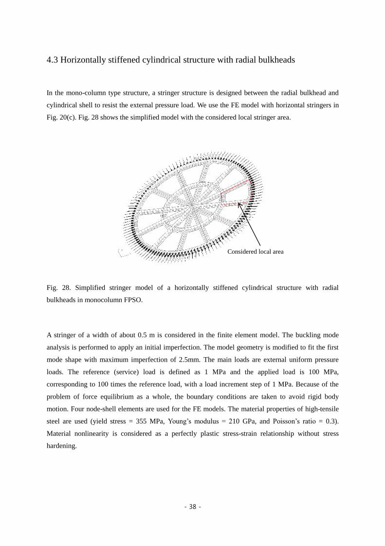
4.3 Horizontally stiffened cylindrical structure with radial bulkheads
In the mono-column type structure, a stringer structure is designed between the radial bulkhead and
cylindrical shell to resist the external pressure load. We use the FE model with horizontal stringers in
Fig. 20(c). Fig. 28 shows the simplified model with the considered local stringer area.
Fig. 28. Simplified stringer model of a horizontally stiffened cylindrical structure with radial
bulkheads in monocolumn FPSO.
A stringer of a width of about 0.5 m is considered in the finite element model. The buckling mode
analysis is performed to apply an initial imperfection. The model geometry is modified to fit the first
mode shape with maximum imperfection of 2.5mm. The main loads are external uniform pressure
loads. The reference (service) load is defined as 1 MPa and the applied load is 100 MPa,
corresponding to 100 times the reference load, with a load increment step of 1 MPa. Because of the
problem of force equilibrium as a whole, the boundary conditions are taken to avoid rigid body
motion. Four node-shell elements are used for the FE models. The material properties of high-tensile
steel are used (yield stress = 355 MPa, Young’s modulus = 210 GPa, and Poisson’s ratio = 0.3).
Material nonlinearity is considered as a perfectly plastic stress-strain relationship without stress
hardening.
Considered local area
- 39 -
Fig. 29 shows the strain energy composition of force and moment components. We can see that the
portion of the force component is dominant in the local strain energy.
The nonlinear analysis solution is converged within the load of 10.76 MPa, which is 10.76 times the
reference load of 1 MPa as shown in Fig. 30. The structure is stable until the global load of 10.76 MPa
because the sign of the second variation of the strain energy is positive. Fig. 31 shows the elastic and
plastic deformations for four applied load levels: 1 MPa, 7 MPa, 10.59 MPa, and 10.76 MPa. The first
yield stress occurs at a load of 7 MPa. This example shows typical material plasticity-driven failure
because the members directly subject to external loads become fully plastic at critical state.
Fig. 32 shows the maximum local load ratio of 10.23 times the local load for the approximated load
method in the stable range. In the norm value method, however, the local load ratio steadily increases,
and is overestimated compared to the approximated load method after the local load ratio of 9.0.
Fig. 33 shows the local load ratio - displacement index curve for both the present and previous
methods [36], and the local safety factors are presented in Table 2. The evaluation through local FE
analysis as the previous study shows much higher safety factor as 2.89 times present method because
this problem is very ductile due to material plasticity.
Fig. 34 shows the local load extraction numbering sequence for the stringer structure. Fig. 35 shows
the local load component plots for the critical load and approximated load at critical step. As the
nonlinearity increases, it can be seen that there is a difference between the critical load and the
approximated load due to the nonlinear behavior, especially in the edge from P13 to P23 which is
directly subject to the external pressure.
Table 2. Local safety factors for a horizontally stiffened cylindrical structure with radial bulkheads.
Direct evaluation through global FE
analysis (Proposed)
Evaluation method through local FE
analysis (Zi et al. 2017 [36])
Horizontal stringer 10.22 29.59

- 40 -
Fig. 29. Strain energy composition of force and moment components for local structural domain of a
horizontally stiffened cylindrical structure with radial bulkheads.
Fig. 30. Second variation of strain energy in local domain of a horizontally stiffened cylindrical
structure with radial bulkheads.
1 MPa
10.76 MPa
(a)
(d)
10.59 MPa
(c)
7 MPa
(b)

- 41 -
Fig. 31. Elastic and plastic deformations (five-time scale) of a stiffened cylindrical shell structure with
radial bulkheads. The applied loads are (a) 1 MPa, (b) 7 MPa, (c) 10.59 MPa, and (d) 10.76 MPa. The
red color indicates that the element has reached the material yield stress.
Fig. 32. Local load ratio - displacement index curve of a horizontally stiffened cylindrical structure
with radial bulkheads.
(a) (b)
(c) (d)
10.23
11.02
Stable
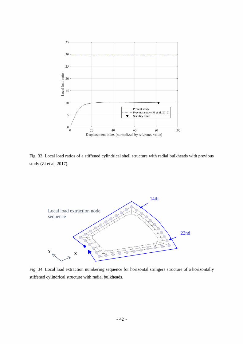
- 42 -
Fig. 33. Local load ratios of a stiffened cylindrical shell structure with radial bulkheads with previous
study (Zi et al. 2017).
Fig. 34. Local load extraction numbering sequence for horizontal stringers structure of a horizontally
stiffened cylindrical structure with radial bulkheads.
Local load extraction node
sequence
Y X
14th
22nd

- 43 -
Fig. 35. Local load component plots (unit: MPa) for the critical load and approximated load at critical
step of a horizontally stiffened cylindrical structure with radial bulkheads.

- 44 -
4.4 Bracket girder in the column-pontoon connection structure of tension leg
platform
The local bracket girder structure in TLP (tension leg platform) hull is selected as the last example,
which has a non-typical geometry not to be applied to the conventional design formula. TLP is a
vertically moored floating structure for deep water as shown in Fig. 36 [41]. The horizontal pontoon
structure is usually connected to the vertical column, which is locally reinforced by a stiffener and a
bracket girder as shown in Fig. 37. Due to the connection geometry between cylindrical column and
box type pontoon, irregular shaped bracket girder structure is attached on the connection area. Since it
is difficult to intuitively estimate a typical deformed shape and stress distribution under the subjected
load, a direct structural response should be analyzed in consideration of the global structural stiffness
through the nonlinear finite element analysis.
(a) (b) (c)
Fig. 36. TLP installed in West Africa field: (a) Photo of TLP [41], (b) schematic of TLP hull with
column and pontoon structures, and (c) plan view of the bracket girder between column and pontoons.
Considered local area
Part model

- 45 -
In the tension leg platform problem, the part of column with adjacent pontoon structure is considered
as the full domain of the finite element analysis as shown in Fig. 37. The local bracket girder structure
of interest is the horizontally irregular-shaped plate between the cylindrical shell plating of the column
and the horizontal girder in the pontoon. The zoomed view of the bracket girder is shown in Fig. 38.
Fig. 37. Finite element model of a column-pontoon connection structure of tension leg platform.
Fig. 38. Finite element model of a bracket girder of interest in the column-pontoon connection
structure of tension leg platform.
TLP Pontoon
TLP Column
Stability evaluation
area (range)

- 46 -
As shown in Fig. 39, the bracket girders are located in vertically as a same design detail, and the
concerned position is selected to the vertically medium level where the local load on bracket girder
boundary is most generated. The initial imperfection of the bracket girder is assumed to be 3.5 mm in
the vertical direction, and the geometry of the finite element model is modified as the lowest local
mode shape. In order to prevent the occurrence of unbalance forces in the considered area, boundary
conditions are specified far away from the target bracket girder. This tension leg platform mainly
experiences the external and internal water head pressure because it is installed at calm sea of West
Africa. Therefore, the inner tank and the external water head pressure are defined as the global
reference (service) load. To investigate the design safety margin, the structural stability of the local
bracket girder structure is evaluated by linearly increasing the global reference load on the column-
pontoon connection structure.
Three and four node-shell elements are used for the FE models. The material properties of high-tensile
steel are used (yield stress = 355 MPa, Young’s modulus = 210 GPa, and Poisson’s ratio = 0.3).
Material nonlinearity is considered as a perfectly plastic stress-strain relationship without stress
hardening.
Fig. 39. Finite element model and applied loads of a bracket girder in the column-pontoon connection
structure of tension leg platform.
Considered local bracket girder structure
External sea pressure
Internal tank pressure

- 47 -
Fig. 40 shows the strain energy composition of force and moment components. We can see that the
portion of the force component is dominant in the local strain energy. As shown in Fig. 41, it is stable
until the external load of 3.5 times reference (service) load since the sign of the second variation of
the strain energy is positive. Fig. 42 shows the elastic and plastic deformations for normalized global
loads of 1.0, 2.0, 3.1, 3.5, 3.8, and 4.0. The first yield occurs at a normalized global load of 2.0 and
most of the area is plastic at a normalized global load of 4.0. This example shows failure that is driven
by combined geometric and material nonlinearities.
At the critical limit state, the bracket girder flange edge is deformed in the lateral direction as shown
in Fig. 43(a). The vertical (z-direction) displacement of the point, at which the maximum
displacement occurs, is plotted along with the external load as shown in Fig. 43(b). In this figure, as
the displacement increases, the external load also continues to increase, and it is not known at what
load step the resistance of the local structure has been reached.
Fig. 44 shows the local load extraction numbering sequence. Fig. 45 shows local load component
plots for the critical load and approximated load at critical step. As the nonlinearity increases, it can be
seen that there is a difference between the critical load and the approximated load due to the nonlinear
behavior
From the local load ratio - displacement index curve, we can find the analysis step with the highest
local load ratio of 3.25 by the approximated load method as shown in Fig. 46. However, from the
result of stability check, the local load ratio of 3.22 is the stable state limit, which is the representative
critical local load ratio. The first instability local load ratio by norm value method is 3.31 which is 2.8%
higher than the one by the approximated load method. After the stable state limit, the local load ratio
by the norm value method doesn’t significantly decrease as a different tendency compared to
approximated method.

- 48 -
Fig. 40. Strain energy composition of force and moment components for local structural domain of a
bracket girder in the column-pontoon connection structure of tension leg platform.
Fig. 41. Second variation of strain energy in local domain of a bracket girder in the column-pontoon
connection structure of tension leg platform.
(a) 1.0 (b) 2.0
(c) 3.1
(d) 3.5
(e) 3.8
(f) 4.0

- 49 -
Fig. 42. Elastic and plastic deformations (three-time scale) of a bracket girder in the column-pontoon
connection structure of tension leg platform. Applied normalized global loads are (a) 1.0, (b) 2.0, (c)
3.1, (d) 3.5, (e) 3.8, and (f) 4.0. The red color indicates that the element has reached the material yield
stress.
(a)
(c)
(e)
(b)
(d)
(f)

- 50 -
(a)
(b)
Fig. 43. Deformation of a bracket girder in the column-pontoon connection structure of tension leg
platform: (a) vertical (z-) direction displacement contour (unit: mm) at critical state and (b) vertical (z-)
direction displacement on point A under the various applied loads.
Y X
Z
A
3.5 (Stability limit)
Globally Stable
Locally Unstable

- 51 -
Fig. 44. Local load extraction numbering sequence of a bracket girder in the column-pontoon
connection structure of tension leg platform.
Local load extraction node sequence
Y
X
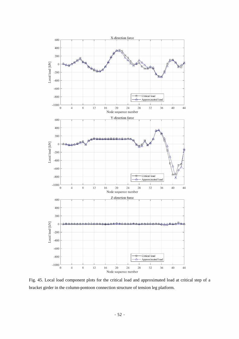
- 52 -
Fig. 45. Local load component plots for the critical load and approximated load at critical step of a
bracket girder in the column-pontoon connection structure of tension leg platform.

- 53 -
Fig. 46. Local load - displacement index curve of a bracket girder in the column-pontoon connection
structure of tension leg platform.
3.22
3.31

- 54 -
Chapter 5. Computational efficiency
In this Chapter, the nonlinear analysis results for the full domain and reduced domain FE models are
reviewed to validate the reliability and applicability of model reduction method. We then apply the
model reduction method to evaluating the stability of local structures for two numerical examples.
Finally, we check the computation efficiency improvement.
5.1 Reliability and applicability of model reduction method
In general, the finite element model of the global structure has many degrees of freedom, but the local
structure may have a relatively a few degree of freedom. In this case, in a computational cost point of
view, it is very useful to condense the stiffness for the degrees of freedom except the region of interest
using the model reduction method [42], and proceed to perform the nonlinear analysis only for the
region of interest as shown in Fig. 47. A condensed stiffness is linear and does not require nonlinear
iterations every time, so the computational cost can be greatly reduced.
The static condensation technique is briefly illustrated in the following derivations. The relationship
between displacements and loads is shown as the static equilibrium equation;
11 12 1 1
21 22 2 2
K K U R
K K U R
, (20)
where K is the stiffness matrix, U is the displacement vector, R is the load vector, and
their subscripts 1 and 2 denote slave (removed) and master (residual) degrees of freedom, respectively.
When the formulation for 2U can be derived as
-1 -1
21 11 12 22 2 21 11 1 2K K K K U K K R R . (21)

- 55 -
We can finally derive the stiffness matrix K and load vector R regarding residual degrees of
freedom of 2U ;
-1
21 11 12 22K K K K K , (22a)
-1
21 11 1 2R K K R R . (22b)
Fig. 47. Schematic of the model reduction method with static condensation for local structural
stability evaluation.

- 56 -
The analysis results for load-carrying structures with nonlinear contact and frictional behaviors
between large floating offshore structures are reviewed to validate the reliability and applicability of
the model reduction method. The evaluation of contact and friction forces on the interface local
connections is conducted by performing nonlinear contact analysis considering the local stiffness and
geometry. The method is applied to the nonlinear behaviors of following interfaces;
Vertical and anti-pitch/roll support interfaces between the FLNG hull and independent tank,
and
Stopper-type sea-fastening interfaces between cargo and transportation barge.
The proposed analysis method is a superelement method with a static condensation technique. A
superelement is a group of finite elements in which part of the DOF is condensed out. Guyan
reduction [43] can be used for the static condensation. The condensation of a large stiffness matrix can
also be performed very quickly by applying an automated static condensation algorithm [44].
Verification of the superelement method using gap elements in MSC/NASTRAN [37] is performed.
Fig. 48 shows a simple FE model used for verification. Yellow beams are modeled as gap elements.
The DOFs in the stiffness matrix of the lower steel box are condensed to the DOF of the gap elements
on the lower and external sides, denoted as superelement No. 10. The DOF of the upper steel box are
condensed to the DOF of the gap elements on the upper and inner sides, denoted as superelement No.
20. A vertical boundary condition is applied on the lower face of the lower box using a vertical spring
to represent restoring behavior in a floating state. The calculated DOF of the full and superelement
models are listed in Fig. 48. Anti-pitch supports are named AP1 and AP2, and vertical supports are
designated VT1 to VT6, as shown in Fig. 49. The loads applied are gravity and longitudinal inertia
load.
Nonlinear analyses of the full FE model and residual gap FE model using superelement method are
performed. The static and slip friction coefficient applied is 0.2. The convergence criteria applied are
EPSP = 1E-3 (error tolerance for load criterion) and EPSW = 1E-5 (error tolerance for work criterion).

- 57 -
Full FE model degrees of freedom
(gap element, lower, and upper steel boxes)
1,740
Superelement model degrees of freedom
Residual
(gap element)
Superelement 10
(lower steel box)
Superelement 20
(upper steel box)
144
1,596 (original) 144 (original)
72 (condensed) 72 (condensed)
Fig. 48. Simple FE model for nonlinear superelement analysis verification.
Fig. 49. Notation of gap elements: ant-pitch (AP) and vertical (VT) elements.
Gap element
(SE00)
Superelement No. 20 (SE20)
Superelement No. 10 (SE10)

- 58 -
Fig. 50 shows that the result of the condensed FE analysis using superelement method coincides with
the one from full FE analysis. The direction of contact force is in line with that of the gap element.
Friction (I) and (II) forces are in two orthogonal directions of contact force. In this analysis, nonlinear
large displacement effects are not considered. Considering the nonlinear large displacement effects,
the results can be different according to the rotational displacement level of the upper steel box. It is
noted that the proposed procedure is only valid in the case that the relative rotational displacement of
the independent object is small.
(a) (b) (c)
Fig. 50. Normalized contact and friction force comparison between full FE model and condensed FE
model using the proposed superelement method (static and slip friction coefficient = 0.2, convergence
criteria: EPSP = 1E−3 and EPSW = 1E−5); (a) contact force, (b) friction(i) force, and (c) friction(ii)
force.

- 59 -
APPLICATION I: FLNG INDEPENDENT CARGO TANK
Membrane type CCS (Cargo Containment System) for LNG (Liquefied Natural Gas) storage is widely
used in LNG carriers and FLNG (Floating Liquefied Natural Gas) projects. The sloshing impact
pressure is one of most critical design loads for the CCS, and many structural issues induced by the
sloshing still remain to the present. To reduce sloshing related issues, another type of CCS which
names as independent type B prismatic tank system is being tried for application to FLNG in a FEED
(Front-End Engineering and Design) project. From a structural safety point of view, independent tank
supports are critical areas because they are load-carrying members; so the reliable evaluation of the
structural strength of the tank supports is required.
Classification Societies [45-48] have proposed applicable evaluation procedures in consideration of
the use of friction coefficients with nonlinear contact behaviors of interface areas of the supports. Fig.
51(a) shows the example of cargo tank supports for vertical and anti-roll. The vertical and anti-pitch
supports are generally arranged on inner bottom of the hull, and anti-roll supports are arranged along
the tank centerline at the top and bottom of the hull. Contact and friction forces act on interface areas
between the tank and hull where the tank contacts the supports, as shown in Figs. 51(b) and 51(c). In
this support configuration, the characteristics of the frictional behavior of their contact, including the
initial gap on supports and static dead loads, result in very complex effects on the support structures.

- 60 -
(a)
(b)
(c)
Fig. 51. Example of independent cargo tank supports [47]: (a) the mid ship section, (b) the vertical
support model and (c) the anti-roll and anti-pitch support models.

- 61 -
In this study, a two-row independent tank type FLNG is considered for evaluation of tank supports.
From the hydrodynamic analysis, the hydrodynamic pressure and inertia load RAOs (Response
Amplitude Operators) are generated. Fig. 52 shows the generated hydrodynamic pressure RAO on the
internal tank and external surface at a certain wave frequency. For the hydrodynamic load generation,
a representative sea state of the Pierson-Moskowitz wave spectrum (significant wave height of 5 m
and peak period of 10.5 s) is selected, which corresponds to a 100-year return period maximum level
in Southeast-Asia gas fields. The irregular hydrodynamic pressure and inertia loads are generated by
superposition of regular load RAOs, at all-time instants during 300 s, with intervals of 0.5 s only for
the applicability check of the proposed method.
Fig. 52. Hydrodynamic and internal tank pressure RAO (LNG tank fully-loaded condition, quartering
sea, ω= 0.398).
Table 3. Stiffness matrix sizes (degrees of freedom) of full and superelement models for FLNG
independent cargo tank.
Full FE model degrees of freedom
(gap element, LNG tank, and hull)
2,729,646
Superelement model degrees of freedom
Residual
(gap element)
Superelement 10
(starboard LNG tank)
Superelement 20
(hull)
1,728
94,014 (original) 2,635,632 (original)
864 (condensed) 864 (condensed)

- 62 -
The DOF in the stiffness matrix of the starboard tank are condensed to the DOF of the gap elements
on the tank side, which is denoted as superelement No. 10. The other adjacent hull structure is
condensed to the DOF of the gap elements on the hull side, which are denoted as superelement No. 20.
The loads generated are condensed to the DOF of both end nodes of the gap elements in the same
manner used for the stiffness matrix. The solving of the residual gap elements is performed with
condensed stiffness matrices and local loads. The calculated DOF of the full and superelement models
are listed in Table 3; those of the full matrix are about 2.7 million. On the other hand, after applying
the condensation technique, the matrix size is dramatically reduced to 864.
The static and slip friction coefficient applied is 0.2, and the stiffness of gap elements are
appropriately estimated to represent the stiffness of the inserted wood and local steel support structure.
It is noted that the values applied for the coefficients and stiffness are selected as appropriate for the
feasibility check of the proposed procedure.
Figs. 53 and 54 show the critical support locations where the highest contact forces occur. All the
critical support locations are at corners, in the case that the stiffness of all the supports are the same.
In an actual design, stiffness optimization is required according to the location of each support. Figs.
55 to 58 show the normal contact force distributions, which are the maximum values during 300 s of
simulation.

- 63 -
Fig. 53. Considered anti-roll support location in a starboard side tank.
Fig. 54. Considered anti-pitch and vertical support locations in a starboard side tank.
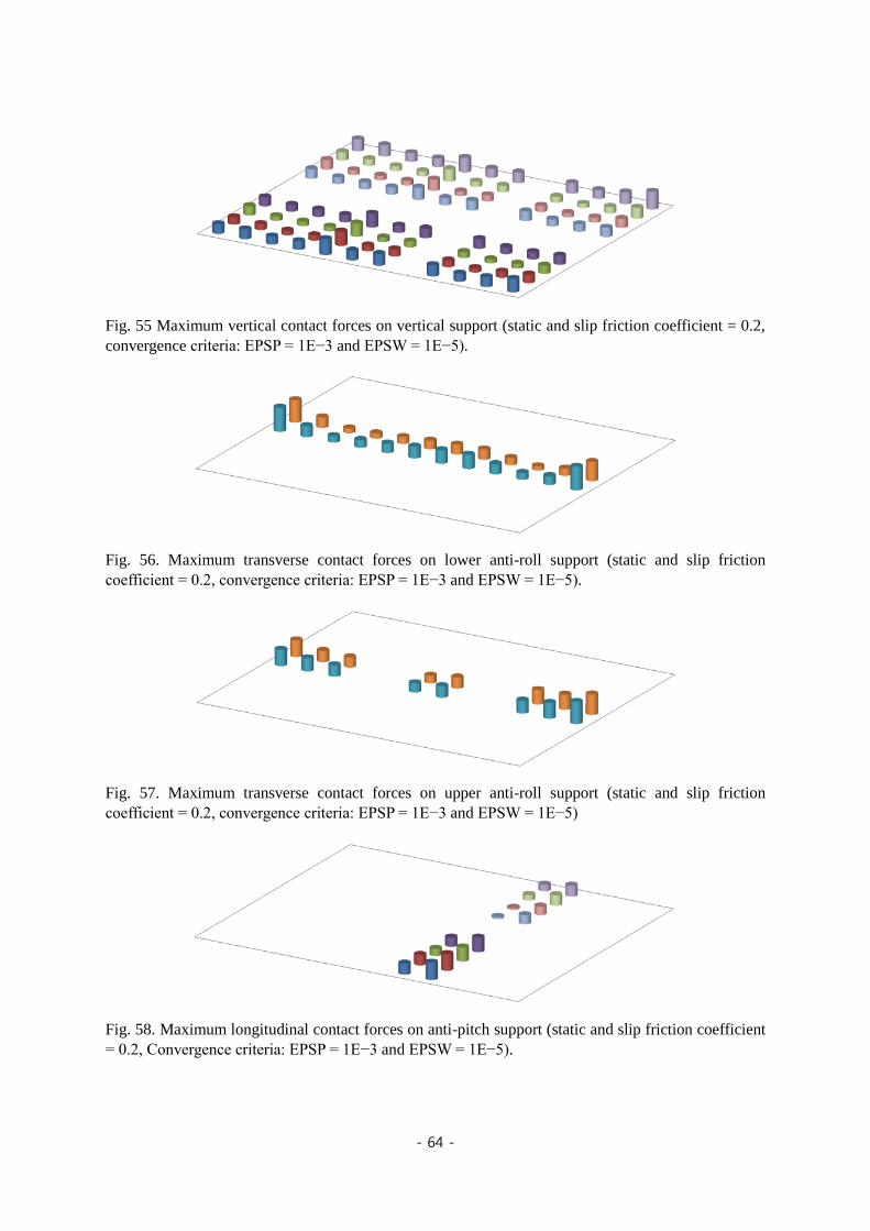
- 64 -
Fig. 55 Maximum vertical contact forces on vertical support (static and slip friction coefficient = 0.2,
convergence criteria: EPSP = 1E−3 and EPSW = 1E−5).
Fig. 56. Maximum transverse contact forces on lower anti-roll support (static and slip friction
coefficient = 0.2, convergence criteria: EPSP = 1E−3 and EPSW = 1E−5).
Fig. 57. Maximum transverse contact forces on upper anti-roll support (static and slip friction
coefficient = 0.2, convergence criteria: EPSP = 1E−3 and EPSW = 1E−5)
Fig. 58. Maximum longitudinal contact forces on anti-pitch support (static and slip friction coefficient
= 0.2, Convergence criteria: EPSP = 1E−3 and EPSW = 1E−5).
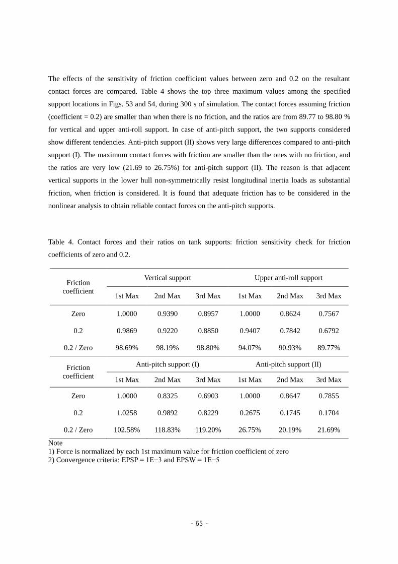
- 65 -
The effects of the sensitivity of friction coefficient values between zero and 0.2 on the resultant
contact forces are compared. Table 4 shows the top three maximum values among the specified
support locations in Figs. 53 and 54, during 300 s of simulation. The contact forces assuming friction
(coefficient = 0.2) are smaller than when there is no friction, and the ratios are from 89.77 to 98.80 %
for vertical and upper anti-roll support. In case of anti-pitch support, the two supports considered
show different tendencies. Anti-pitch support (II) shows very large differences compared to anti-pitch
support (I). The maximum contact forces with friction are smaller than the ones with no friction, and
the ratios are very low (21.69 to 26.75%) for anti-pitch support (II). The reason is that adjacent
vertical supports in the lower hull non-symmetrically resist longitudinal inertia loads as substantial
friction, when friction is considered. It is found that adequate friction has to be considered in the
nonlinear analysis to obtain reliable contact forces on the anti-pitch supports.
Table 4. Contact forces and their ratios on tank supports: friction sensitivity check for friction
coefficients of zero and 0.2.
Friction
coefficient
Vertical support Upper anti-roll support
1st Max 2nd Max 3rd Max 1st Max 2nd Max 3rd Max
Zero 1.0000 0.9390 0.8957 1.0000 0.8624 0.7567
0.2 0.9869 0.9220 0.8850 0.9407 0.7842 0.6792
0.2 / Zero 98.69% 98.19% 98.80% 94.07% 90.93% 89.77%
Friction
coefficient
Anti-pitch support (I) Anti-pitch support (II)
1st Max 2nd Max 3rd Max 1st Max 2nd Max 3rd Max
Zero 1.0000 0.8325 0.6903 1.0000 0.8647 0.7855
0.2 1.0258 0.9892 0.8229 0.2675 0.1745 0.1704
0.2 / Zero 102.58% 118.83% 119.20% 26.75% 20.19% 21.69%
Note
1) Force is normalized by each 1st maximum value for friction coefficient of zero
2) Convergence criteria: EPSP = 1E−3 and EPSW = 1E−5

- 66 -
APPLICATION II: OFFSHORE DRY TRANSPORTATION
Recently, large offshore structures are frequently transported while loaded on transportation barges
(i.e., dry transportation). Compared with wet towing, the load applied to the cargo structure is smaller
because it does not directly encounter wave loads. In terms of transportation cost, it is advantageous
because the transportation period is relatively short due to faster towing speed, compared to wet
towing. To secure the cargo structure during dry transportation, sea-fastening designs should be
considered. Conventionally, an offshore jacket or topside platform structure is often dry-transported.
The design of sea-fastening can be conducted by hand calculation or spread sheet because of the
simple point contacts between the framed cargo structure and the barge. However, in recent years,
plated structures such as FPU (floating production unit), cylindrical FPSO (floating production
storage and offloading), and Spar hull are also being dry-transported. Because of the surface contact
between the plated cargo structure and the transportation barge, the friction between them should
definitely be considered in the sea-fastening design. Friction force depends on the global and local
structural deformation of the contact areas. The mutual contact and frictional behaviors of a complex
plated structure cannot be determined using simple calculations, but can be evaluated by performing
nonlinear FE analysis.
An offshore dry transportation analysis is performed as a second application in this section. Fig. 59
shows the FE model of dry transportation. The model includs a cargo structure, wedge-type large
auxiliary structures, cribbing wood, and the transportation barge. Fig. 60 shows the detailed view of
the gap elements, longitudinal and transverse stoppers for two representative areas. The analysis
consists of two similar load cases that include static gravity, hydrodynamic inertia load, and external
pressures. Fig. 61 shows the deformed shape of full-ship nonlinear FE analysis, considering horizontal
contact behavior with gap elements, for a specific load case. The cargo is overhung in the longitudinal
direction. It is expected that longitudinal friction is considerable from the deformed shape; however,
the vertical cribbing wood is not expected to be slip, and was linearly modeled. This is because the
applied horizontal inertia load of the overall cargo is less than the overall horizontal friction in this
study.

- 67 -
Fig. 59. Overall FE model of dry transportation.
(a)
(b)
Fig.60. Detailed view of sea-fastening stopper and gap elements between cargo and transportation
barge: (a) plated structure and (b) vertical columns.
Plated
structure Vertical columns

- 68 -
Fig.61. Deformed shape of dry transportation model for load case 2.
The superelement analysis is performed in the same manner as for the FLNG independent tank
support. Gap elements on the horizontal stoppers are assigned residual DOF and all the other elements
of cargo, auxiliary, and barge structures are considered to remove DOF. The sizes of the matrices
considered (for DOF) of a full FE model and reduced model, are shown in Table 5.
Table 5. Stiffness matrix sizes (degrees of freedom) of full and superelement models for dry
transportation.
Full FE model
(gap element, cargo, and barge)
3,067,356
Superelement model
Residual
(gap element)
Superelement 10
(cargo and barge)
1,968
3,067,356 (original)
1,968 (condensed)

- 69 -
The validity of the proposed superelement analysis is checked as shown in Table 6. The static and slip
friction coefficient applied is 0.2, and the stiffness of gap elements are appropriately estimated to
represent the stiffness of the local steel stopper structure. The maximum contact forces are compared
with the ones from full FE analysis for two load cases. The largest difference in the contact forces is
just 2.63E-6, i.e., nearly negligible, at a longitudinal stopper. A comparison of computing time is
shown in Table 7. The processor of the computer used was a GenuineIntel / 1699 MHz. The full FE
analysis of 3.1 million of DOF for the two load cases studied, required 13.67 h. However, the
superelement analysis for 1,968 DOF requires only 43 s. Prior to this, pre-processing time of 7.25
hours is required for stiffness and load condensation. If a large number of load cases are considered to
obtain load responses against fatigue load time history, the efficiency of the proposed calculation
approach will be very high compared to full FE analysis.
Table 6. Comparison of maximum contact forces of full and superelement analysis for dry
transportation.
Load Case Location Full FE * Superelement * Difference ratio
1 Longitudinal stopper 1.0 1.0 0
Transverse stopper 1.0 1.00000263 2.63E-6
2 Longitudinal stopper 1.0 1.0 0
Transverse stopper 1.0 1.0 0
Note
1) * Contact force is normalized by each full FE analysis result
2) Static and slip friction coefficient = 0.2
3) Convergence criteria: EPSP=1E-3 and EPSW=1E-5
Table 7. Comparison of computing time of full and superelement nonlinear analysis for dry
transportation.
Full FE Superelement
Iterative solving Static condensation Iterative solving
13.67 hours 7.25 hours 43 seconds
Note
1) System: GENUINEINTEL / 1699MHZ / RAM 62GB
2) Platform: INTEL LINUX 2.6.16.60-0.21
3) Static and slip friction coefficient = 0.2
4) Convergence criteria: EPSP=1E-3 and EPSW=1E-5
- 70 -
The accuracy and computing cost of the proposed superelement analysis method were investigated for
use in time consuming analysis. By applying the model reduction method, we confirmed that the
contact behavior and the friction effect were well-reflected.
In the FLNG independent cargo tank support analysis case, the sensitivity of the friction effect of
supports was investigated. If friction was considered (friction coefficient = 0.2), the maximum contact
forces decreased to about one-quarter or one-fifth of the ones for no friction case, for a certain anti-
pitch support. The friction at the contact interface seriously affected the magnitude of contact force
according to the support location. Therefore, adequate friction had to be considered to obtain reliable
contact forces on the independent tank supports.
In the case of contact force, accuracy was guaranteed with 2.63E-6 of error ratio, which was observed
in the dry transportation load cases considered. Superelement analysis could reliably be considered to
reflect both global and local behaviors. The full FE analysis considered millions of DOF while
superelement analysis considered only thousands of DOF. In terms of calculation efficiency, full ship
FE analysis required 13.67 h and superelement analysis required only 43 s, aside from the static
condensation work.
In the nonlinear large displacement problem, the accuracy of nonlinear contact results might be
reduced because the condensed stiffness matrix was not updated along with the variation of stiffness
induced by geometric nonlinearity. The result was valid for the calculation of small displacement
problems.
Many load cases needed to be considered during structural design. Occasionally, full ship FE analyses
were required to evaluate the global structural strength. When repeated analyses were required due to
design changes during actual offshore project design development, nonlinear full ship analysis was
not applicable. From this study, however, it was found that the proposed superelement analysis with
static condensation was quite applicable for a particular nonlinear contact problem, and had the
advantage of short calculation time.
- 71 -
5.2 Comparisons with reduced domain analyses
In this section, the structural stability is evaluated by the reduced model analysis for the two examples
in Chapter 4, and compared with the results of the full domain analysis.
5.2.1 Horizontally stiffened cylindrical structure with radial bulkheads
We evaluate the structural stability by applying the model reduction method for the local stringer part
considered in section 4.3. Two cases are evaluated for different ranges of nonlinear analysis. The one
is the stringer region of interest, and the other is the extended range of the stringer with adjacent
bulkheads in order to improve the accuracy of the analysis result. The stiffness of all other areas
except the selected area is condensed. The model reduction method uses both the stiffness of the part
of interest and the condensed stiffness of the other part.
The structural stability is also evaluated by applying linear increment of initial prescribed
displacement, which is commonly applied in previous studies [35, 36]. The prescribed displacement
analysis method uses only a stiffness of the part of interest. In this way, the results of the model
reduction and prescribed displacement cases are compared with the full domain analysis in this
section.
As shown in Fig. 62, the nonlinear analysis is performed only for the stringer region of interest with
the model reduction of the other region. In addition, the analysis is performed by incrementing
prescribed displacement at the initial reference load application. Fig. 63 shows the extended nonlinear
analysis domain with the extended model reduction.
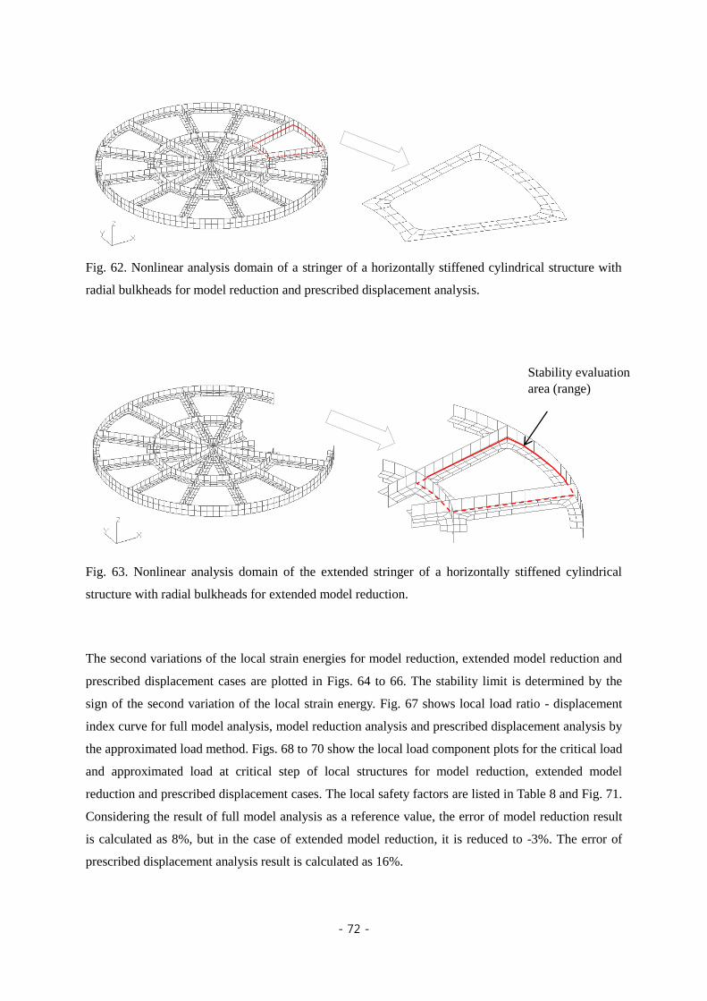
- 72 -
Fig. 62. Nonlinear analysis domain of a stringer of a horizontally stiffened cylindrical structure with
radial bulkheads for model reduction and prescribed displacement analysis.
Fig. 63. Nonlinear analysis domain of the extended stringer of a horizontally stiffened cylindrical
structure with radial bulkheads for extended model reduction.
The second variations of the local strain energies for model reduction, extended model reduction and
prescribed displacement cases are plotted in Figs. 64 to 66. The stability limit is determined by the
sign of the second variation of the local strain energy. Fig. 67 shows local load ratio - displacement
index curve for full model analysis, model reduction analysis and prescribed displacement analysis by
the approximated load method. Figs. 68 to 70 show the local load component plots for the critical load
and approximated load at critical step of local structures for model reduction, extended model
reduction and prescribed displacement cases. The local safety factors are listed in Table 8 and Fig. 71.
Considering the result of full model analysis as a reference value, the error of model reduction result
is calculated as 8%, but in the case of extended model reduction, it is reduced to -3%. The error of
prescribed displacement analysis result is calculated as 16%.
Stability evaluation
area (range)

- 73 -
Fig. 72 shows local load component plots for the critical load and approximated load at critical step
for all analyses. Table 9 and Fig. 73 show the standard errors of the local load distributions compared
to the one of the full model analysis. The smallest value is 42 kN which is the standard error of the
extended model reduction result at maximum local load ratio. In other words, it can be said that the
local load distribution of the extended model reduction case is most similar to full model analysis. The
prescribed displacement analysis shows large error value as 195 kN. When we consider the computing
cost, the extended model reduction case is the best way to represent the local load distribution among
the reduced domain analysis cases.

- 74 -
Fig. 64. Second variation of strain energy in local domain of a horizontally stiffened cylindrical
structure with radial bulkheads for model reduction case.
Fig. 65. Second variation of strain energy in local domain of a horizontally stiffened cylindrical
structure with radial bulkheads for extended model reduction case.

- 75 -
Fig. 66. Second variation of strain energy in local domain of a horizontally stiffened cylindrical
structure with radial bulkheads for prescribed displacement case.
Fig. 67. Local load ratio – displacement index curve of a horizontally stiffened cylindrical structure
with radial bulkheads for all analysis cases.
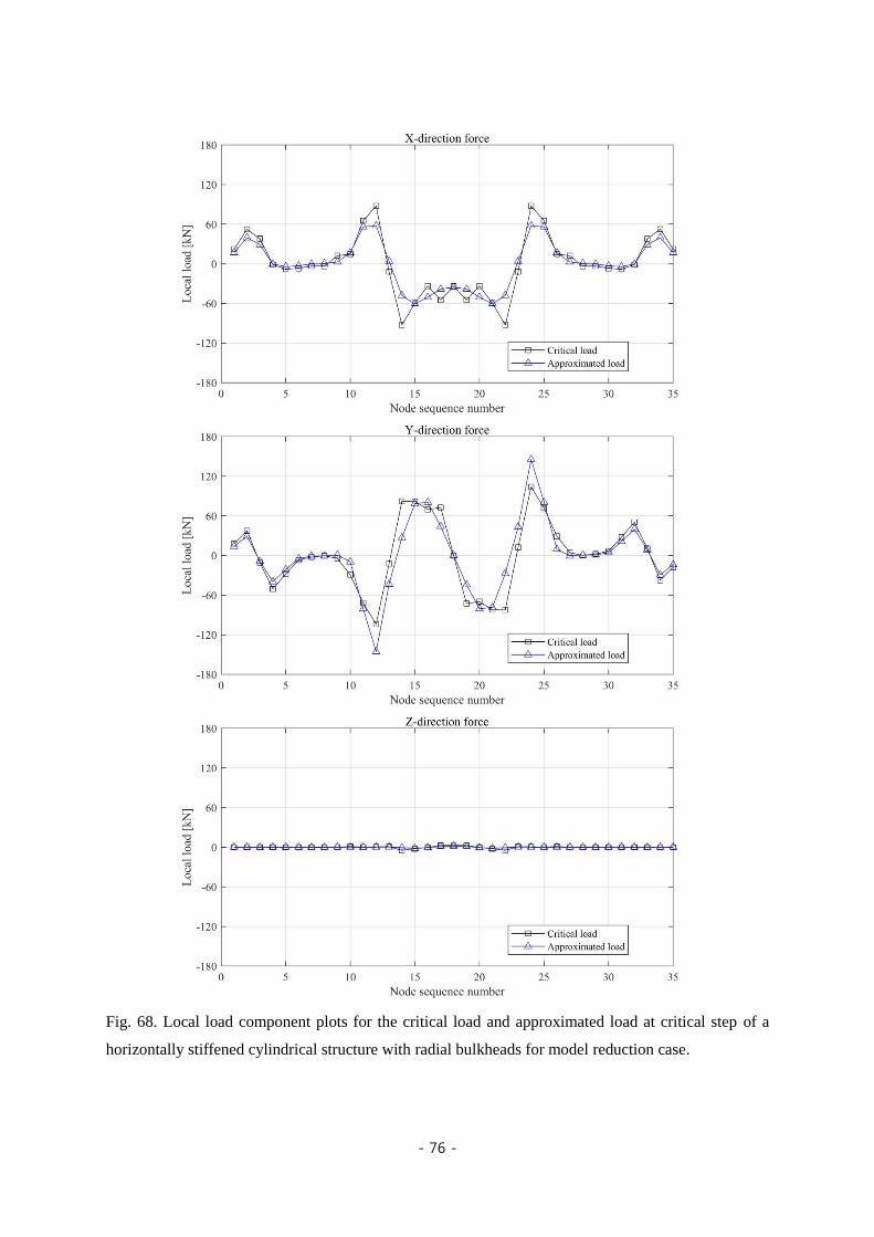
- 76 -
Fig. 68. Local load component plots for the critical load and approximated load at critical step of a
horizontally stiffened cylindrical structure with radial bulkheads for model reduction case.

- 77 -
Fig. 69. Local load component plots for the critical load and approximated load at critical step of a
horizontally stiffened cylindrical structure with radial bulkheads for extended model reduction case.
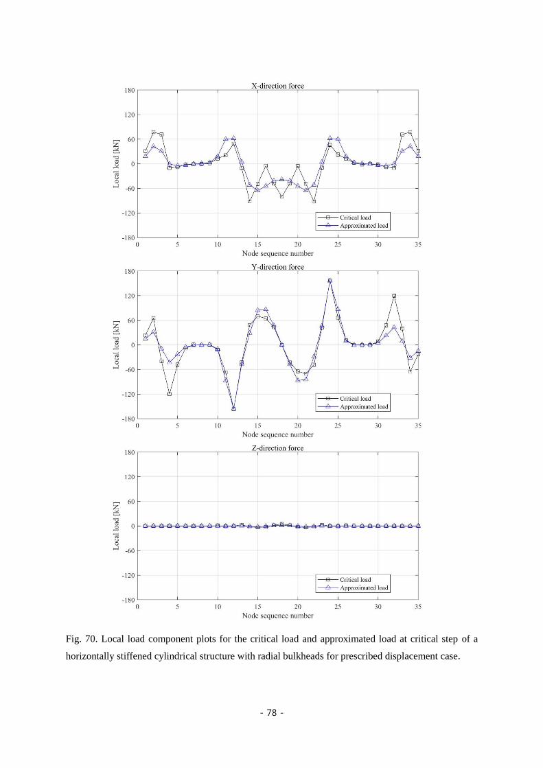
- 78 -
Fig. 70. Local load component plots for the critical load and approximated load at critical step of a
horizontally stiffened cylindrical structure with radial bulkheads for prescribed displacement case.

- 79 -
Table 8. Local safety factors (LSF) of a horizontally stiffened cylindrical structure with radial
bulkheads for all analysis cases.
Full domain Model reduction
Extended
model reduction
Prescribed
displacement
LSF 10.22 11.03 9.95 11.84
Normalized LSF 1.00 1.08 0.97 1.16
Fig. 71. Local safety factors of a horizontally stiffened cylindrical structure with radial bulkheads for
all analysis cases.
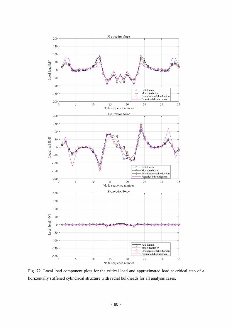
- 80 -
Fig. 72. Local load component plots for the critical load and approximated load at critical step of a
horizontally stiffened cylindrical structure with radial bulkheads for all analysis cases.

- 81 -
Table 9. Standard errors of critical local load of reduced domain analyses compared to full domain
analysis for a horizontally stiffened cylindrical structure with radial bulkheads (unit: kN).
Model reduction
Extended
model reduction
Prescribed
displacement
Standard error of local load * 120 42 195
* Standard error is defined as ( ) ( )f f f fi i ref i i ref , where fi is i-th local load vector and
( )fi ref is i-th local load vector in full domain analysis as the reference value.
Fig. 73 Standard errors of critical local load of reduced domain analyses compared to critical full
domain analysis of a horizontally stiffened cylindrical structure with radial bulkheads. Standard error
is defined as ( ) ( )f f f fi i ref i i ref , where fi is i-th local load vector and ( )fi ref is i-th local
load vector in full domain analysis as the reference value.

- 82 -
5.2.2 Bracket girder in the column-pontoon connection structure of tension leg platform
We evaluate the structural stability by applying the model reduction method for the local bracket
girder part considered in section 4.4. As shown in Fig. 74, the nonlinear analysis is performed only for
the bracket girder region of interest. Two analyses cases are performed, which are the model reduction
of the remaining regions and the prescribed displacement increment based on the reference
displacement. Fig. 75 shows the extended the nonlinear analysis domain for the extended model
reduction.
Figs. 76 to 78 show the second variation of the strain energy for model reduction, extended model
reduction and prescribed displacement cases. Fig. 79 shows local load ratio - displacement index
curve for full model analysis, model reduction analysis and prescribed displacement analysis. Figs. 80
to 82 show the local load component plots for the critical load and approximated load at critical step
of local structures for model reduction, extended model reduction and prescribed displacement cases.
The local safety factor values by the approximated load method are listed in Table 10 and Fig. 83.
Considering the result of full model analysis as a reference value, the error of model reduction result
is calculated as 12%, but in the case of extended model reduction, it is reduced to -6% error. The error
of prescribed displacement analysis result is 4%, which is the lowest. However, there is an unrealistic
result that it becomes stable in the next step immediately after the first instability of the local structure
occurs at the prescribed displacement analysis case as shown in Fig. 78. We can see that the
prescribed displacement analysis case may give a somewhat unstable result and its critical local load
ratio is calculated to be quite low compared to the maximum local load ratio in Figs. 79 and 83.
Therefore, the extended model reduction case gives a rather reliable result among the reduced analysis
cases.
Fig. 84 shows local load component plots for the critical load and approximated load at critical step
for all analyses. Table 11 and Fig. 85 show the standard errors of the local load distributions compared
to the one of the full model analysis. The smallest value is 231 kN which is the standard error of the
extended model reduction result at maximum local load ratio. In other words, it can be said that the
local load distribution of the extended model reduction case is most similar to full model analysis. The
prescribed displacement analysis shows large error value as 394 kN. Similarly in this example, the
extended model reduction case is the best way to represent the local load distributions among the
reduced domain analysis cases.
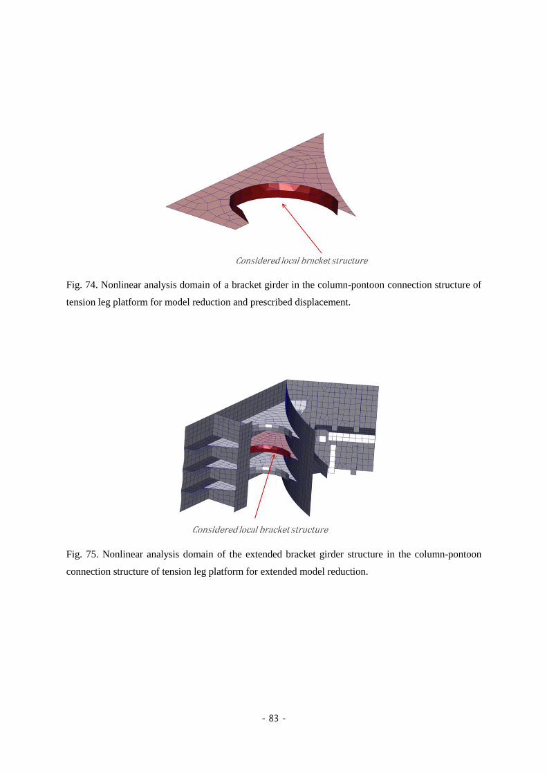
- 83 -
Fig. 74. Nonlinear analysis domain of a bracket girder in the column-pontoon connection structure of
tension leg platform for model reduction and prescribed displacement.
Fig. 75. Nonlinear analysis domain of the extended bracket girder structure in the column-pontoon
connection structure of tension leg platform for extended model reduction.
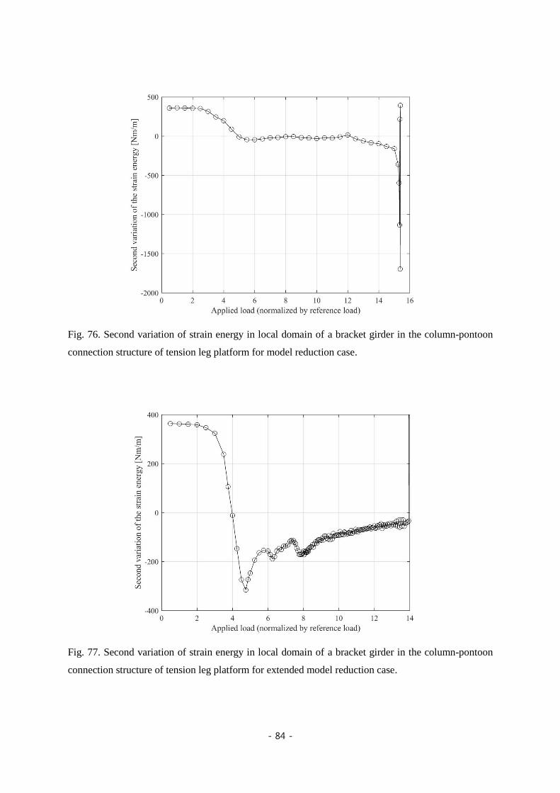
- 84 -
Fig. 76. Second variation of strain energy in local domain of a bracket girder in the column-pontoon
connection structure of tension leg platform for model reduction case.
Fig. 77. Second variation of strain energy in local domain of a bracket girder in the column-pontoon
connection structure of tension leg platform for extended model reduction case.
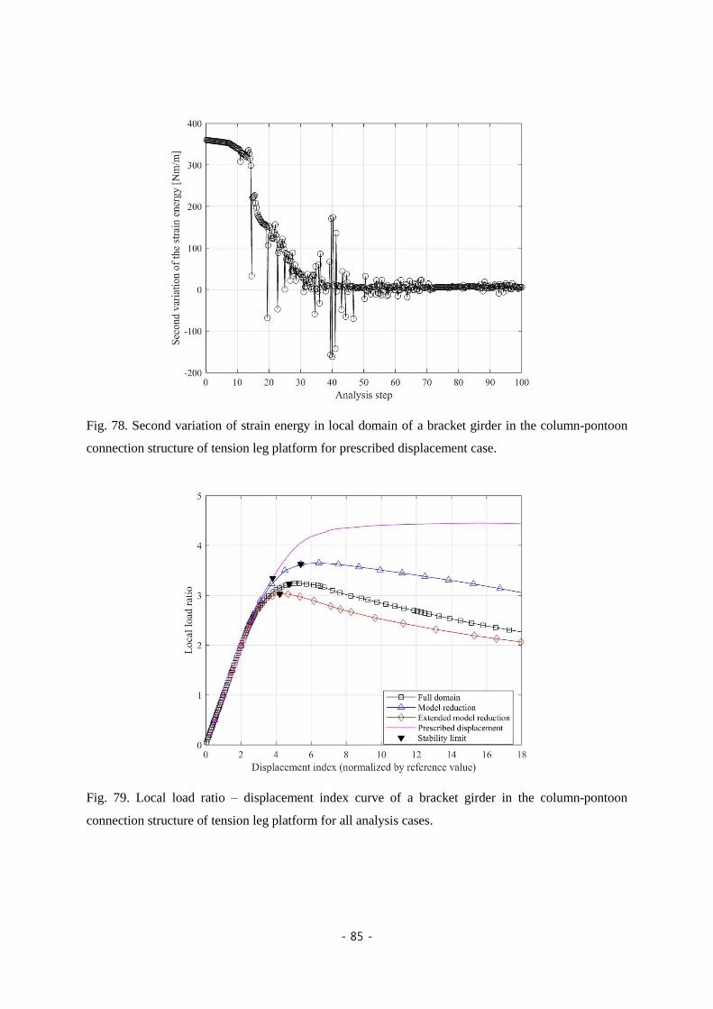
- 85 -
Fig. 78. Second variation of strain energy in local domain of a bracket girder in the column-pontoon
connection structure of tension leg platform for prescribed displacement case.
Fig. 79. Local load ratio – displacement index curve of a bracket girder in the column-pontoon
connection structure of tension leg platform for all analysis cases.

- 86 -
Fig. 80. Local load component plots for the critical load and approximated load at critical step of a
bracket girder in the column-pontoon connection structure of tension leg platform for model reduction
case.

- 87 -
Fig. 81. Local load component plots for the critical load and approximated load at critical step of a
bracket girder in the column-pontoon connection structure of tension leg platform for extended model
reduction case.

- 88 -
Fig. 82. Local load component plots for the critical load and approximated load at critical step of a
bracket girder in the column-pontoon connection structure of tension leg platform for prescribed
displacement case.
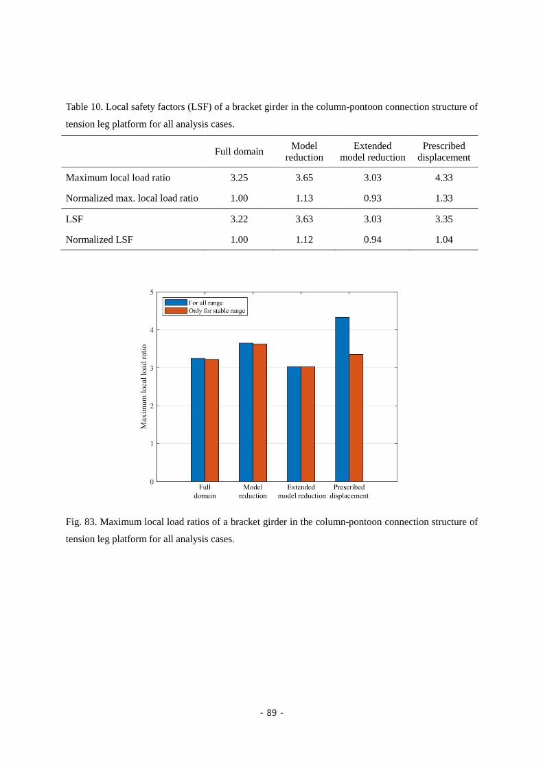
- 89 -
Table 10. Local safety factors (LSF) of a bracket girder in the column-pontoon connection structure of
tension leg platform for all analysis cases.
Full domain
Model
reduction
Extended
model reduction
Prescribed
displacement
Maximum local load ratio 3.25 3.65 3.03 4.33
Normalized max. local load ratio 1.00 1.13 0.93 1.33
LSF 3.22 3.63 3.03 3.35
Normalized LSF 1.00 1.12 0.94 1.04
Fig. 83. Maximum local load ratios of a bracket girder in the column-pontoon connection structure of
tension leg platform for all analysis cases.
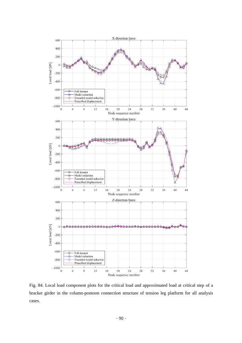
- 90 -
Fig. 84. Local load component plots for the critical load and approximated load at critical step of a
bracket girder in the column-pontoon connection structure of tension leg platform for all analysis
cases.
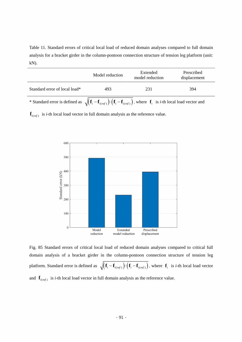
- 91 -
Table 11. Standard errors of critical local load of reduced domain analyses compared to full domain
analysis for a bracket girder in the column-pontoon connection structure of tension leg platform (unit:
kN).
Model reduction
Extended
model reduction
Prescribed
displacement
Standard error of local load* 493 231 394
* Standard error is defined as ( ) ( )f f f fi i ref i i ref , where fi is i-th local load vector and
( )fi ref is i-th local load vector in full domain analysis as the reference value.
Fig. 85 Standard errors of critical local load of reduced domain analyses compared to critical full
domain analysis of a bracket girder in the column-pontoon connection structure of tension leg
platform. Standard error is defined as ( ) ( )f f f fi i ref i i ref , where fi is i-th local load vector
and ( )fi ref is i-th local load vector in full domain analysis as the reference value.

- 92 -
5.3 Computational efficiency improvement
In this section, we check the computing efficiency. If we are interested only in the local structure, it is
very economical to perform nonlinear analysis only for the effective local domain rather than
calculating the nonlinear behavior of the global structure.
The required computing time is measured for each evaluation method by the model reduction and the
prescribed displacement. The evaluation method by the model reduction takes time in the static
condensation process. The extended model reduction case provides the most reliable result among the
reduced domain analyses as shown in Table 11 because the standard error of the extended model
reduction case is smallest. Also, the time required for the analysis of the local region is reduced to
11.9% (=240/2,023) compared to the full domain as shown in Table 12 and Fig. 86.
Table 12. Computing costs of evaluation domains for a bracket girder in the column-pontoon
connection structure of tension leg platform for all analysis cases.
Item Full
domain
Model
reduction
Extended
model reduction
Prescribed
displacement
Number
of nodes
Residual model 37,809 159 2,423 159
Condensed interface 44 263
Time
(seconds)
Condensation 16 54
Iterative run 2,023 9 186 16
Total 2,023 25 240 16
System: GenuineIntel / 2600 MHz / RAM 251GB
Platform: Intel linux 3.10.0-693.el7.x86_64
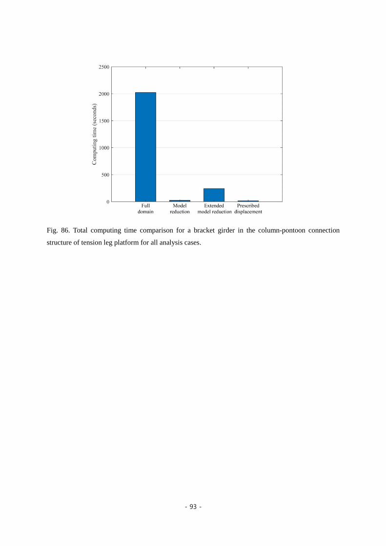
- 93 -
Fig. 86. Total computing time comparison for a bracket girder in the column-pontoon connection
structure of tension leg platform for all analysis cases.

- 94 -
Chapter 6. Concluding remarks
In this thesis, a structural stability evaluation method for local structures was developed by
investigating the second variation of the local strain energy. The method could be practically used to
various arbitrarily shapes of slender local structures for ship and offshore structures by engineers in
industries without much effort. The practical effectiveness of this method was demonstrated through
numerical examples.
In the proposed method, complicated interactions between local and global structures were fully
considered through global nonlinear FE analysis. The instability of the local structure was explicitly
identified even if the overall structural integrity was maintained. The local resistance capacity could
be precisely quantified by the local safety factor. When the target local structure lost stability, the
corresponding magnitude of the external force acting on the global structure could be calculated. Also,
where local buckling occurred in the global structure, i.e., locally damaged area, was easily identified.
A method of calculating the safety factor of any arbitrary shape of the local structure was originally
proposed. The local load of the local structure was approximated by the least-squares fitting method to
quantify the structural safety factor. This approach was very effective for any arbitrarily geometric
shape of the local structure. Quantifying single scalar loads, by averaging or integrating the load
distribution of local structures, could not be applied to arbitrary shapes, but this method was not
limited to being used for any shape.
In the industry, reducing the time required to evaluate structural stability is one of the most important
factors in structural design. For large FE models, the analysis time could be reduced economically
through the model reduction method. The nonlinear iterative solving was performed only for the local
structure in the method. The reliability and computational efficiency were investigated and it was
found that the extended model reduction method was the best solution when the nonlinear analysis
with a full FE model could not be performed due to the limited time.

- 95 -
In future studies, this practical evaluation method can be applied to demonstrate strength proofs of
irregularly reinforced structures and weakened plate openings that are not predefined in design
formulas. In addition, the residual strength and damaged area can be identified to determine the
reinforcement of local structures after structural damages from grounding or collision accidents.

- 96 -
Bibliography
[1] https://en.wikipedia.org/wiki/I-35W_Mississippi_River_bridge
[2] Chakrabarti, S. (2005), Handbook of Offshore Engineering. Elsevier, Kidlington, U.K.
[3] DNVGL (2015), DNVGL-CG-0128. Class Guideline: Buckling; DNVGL.
[4] DNVGL (2018), DNVGL-RU-SHIP Pt.3 Ch.8. Rules for Classification: Buckling; DNVGL.
[5] BV (2018), Rule Note NI 615 DT R02 E. Buckling Assessment of Plated Structures; Bureau
Veritas, Paris, France.
[6] AISC (2016), ANSI/AISC 360-16. An American National Standard: Specification for Structural
Steel Buildings; American Institute of Steel Construction, Chicago, U.S.A.
[7] API (2014), RP 2A-WSD. Recommended Practice for Planning, Designing and Constructing
Fixed Offshore Platforms- Working Stress Design; American Petroleum Institute, Washington, U.S.A.
[8] DNVGL (2017), DNVGL-RP-C202. Recommended Practice: Buckling Strength of Shells;
DNVGL.
[9] DNV (2010), DNV-RP-C201. Recommended Practice: Buckling Strength of Plated Structures; Det
Norske Veritas.
[10] ABS (2018), Guide for Buckling and Ultimate Strength Assessment for Offshore Structures;
American Bureau of Shipping, New York, U.S.A.
[11] Yao, T. and Fujikubo, M. (2016), Buckling and Ultimate Strength of Ship and Ship-Like Floating
Structures. Elsevier Inc., New York, U.S.A.
[12] Paik, J.K. (2018), Ultimate Limit State Analysis and Design of Plated Structures, 2nd Edition.
Jon Wiley & Sons, Chichester, U.K.

- 97 -
[13] Wang, C.M. and Liew, K.M. (1994), “Buckling of triangular plates under uniform compression”,
Eng.Struct., 16(1), 43–50.
[14] Xiang, Y., Wang, C.M., Kitipornchai, S. and Liew, K.M. (1994), “Buckling of triangular Mindlin
plates under isotropic in-plane compression”, ActaMech., 102(1–4), 123–135.
[15] Jaunky, N., Knight, N.F. and Ambur, D.R. (1995), “Buckling analysis of general triangular
anisotropic plates using polynomials”, AIAA J., 33(12), 9387–2654.
[16] Xiang, Y. (2002), “Buckling of triangular plates with elastic edge constraints”, ActaMech.,
156(1–2), 63–77.
[17] Aung, T.M. (2006), “Plastic Buckling of Mindlin Plates”, PhD Dissertation. National University
of Singapore, Singapore.
[18] Lee, S.E., Thayamballi, A.K. and Paik, J.K. (2015), “Ultimate strength of steel brackets in ship
structures”, Ocean Eng. 101, 182–200.
[19] Tham, L.G. and Szeto, H.Y. (1990), “Buckling analysis of arbitrarily shaped plates by spline
finite strip method”, Computers & Structures, 36(4), 729-735.
[20] Wang, C.M., Xiang, Y., Kitipornchai, S. and Liew, K.M. (1994). “Buckling solutions for Mindlin
plates of various shapes”, Eng. Struct., 16(2), 119–127.
[21] Jaunky, N., Knight, N.F. and Ambur, D.R. (1995), “Buckling of arbitrary quadrilateral anisotropic
plates”, AIAA J., 33(5), 938-944.
[22] Saadatpour, M.M., Azhari, M. and Bradford, M.A. (1998), “Buckling of arbitrary quadrilateral
plates with intermediate supports using the Galerkin method”, Computer Methods in Applied
Mechanics and Engineering, 164(3–4), 297-306.
[23] Wu, L. and Feng, W. (2003), “Differential cubature method for buckling analysis of arbitrary
quadrilateral thick plates”, Struct. Eng. Mech., 16(3), 259-273.
[24] Jamshidi, S. and Fallah, N. (2019), “Buckling analysis of arbitrary point-supported plates using
new hp-cloud shape functions”, Struct. Eng. Mech., 70(6), 711-722.

- 98 -
[25] Brubak, L., Hellesland, J. and Steen, E. (2007), “Semi-analytical buckling strength analysis of
plates with arbitrary stiffener arrangements”, Journal of Constructional Steel Research, 63(4), 532-543.
[26] Brubak, L. and Hellesland, J. (2007b), “Approximate buckling strength analysis of arbitrarily
stiffened, stepped plates”, Engineering Structures, 29(9), 2321-2333.
[27] Kim, H.S., Park, Y.M., Kim, B.J. and Kim, K. (2018), “Numerical investigation of buckling
strength of longitudinally stiffened web of plate girders subjected to bending”, Struct. Eng. Mech.,
65(2), 141-154.
[28] Kim, H.S., Park, Y.M., Kim, K. and Choi, B.H. (2019), “Web bend-buckling strength of plate
girders with two longitudinal web stiffeners”, Struct. Eng. Mech., 69(4), 383-397.
[29] Muhammad, T. and Singh, A.V. (2005), “The buckling of rectangular plates with opening using a
polynomial method”, Struct. Eng. Mech., 21(2), 151-168.
[30] Komur, M.A. and Sonmez, M. (2008), “Elastic buckling of perforated plates subjected to linearly
varying in-plane loading”, Struct. Eng. Mech., 28(3), 353-356.
[31] Kim, U.N., Choe, I.H. and Paik, J.K. (2009), “Buckling and ultimate strength of perforated plate
panels subject to axial compression: experimental and numerical investigations with design
formulations”, Ships and Offshore Structures, 4(4), 337-361.
[32] Kim, J.H., Jeon, J.H., Park, J.S., Seo, H.D., Ahn, H.J. and Lee, J.M. (2015), “Effect of
reinforcement on buckling and ultimate strength of perforated plates”, International Journal of
Mechanical Sciences, 92, 194-205.
[33] Saad-Eldeen, S., Garbatov, Y.C. and Soares, G. (2016), “Experimental strength assessment of
thin steel plates with a central elongated circular opening”, Journal of Constructional Steel Research,
118, 135-144.
[34] Mohammadzadeh, B., Choi, E. and Kim, W.J. (2018), “Comprehensive investigation of buckling
behavior of plates considering effects of holes”, Struct. Eng. Mech., 68(2), 261-275.
[35] DNVGL (2016), DNVGL-RP-C208. Recommended Practice: Determination of Structural
Capacity by Non-linear Finite Element Analysis Methods; DNVGL.

- 99 -
[36] Zi, G., Kim, H.H., Ahn, J.Y. and Oh, M.H. (2017), “Evaluation of buckling strength of non-
structured plates by using the deformation energy”, Journal of the Korea Institute for Structural
Maintenance and Inspection, 21(3), 102-113.
[37] MSC Software (2014), MSC Nastran 2014 Quick Reference Guide. MSC Software, Newport
Beach, U.S.A.
[38] Bazant, Z.P. and Cedolin, L. (1991), Stability of Structures: Elastic, Inelastic, Fracture, and
Damage Theories. Oxford University Press, New York, U.S.A.
[39] Kim, D.K., Poh, B.Y., Lee, J.R. and Paik, J.K. (2018), “Ultimate strength of initially deflected
plate under longitudinal compression: Part I = An advanced empirical formulation”, Struct. Eng.
Mech., 68(2), 247-259.
[40] Lei, Y., Chen, S., Wang, L. and Xu, H. (2018), “Global strength analysis of a monocolumn
FPSO”, The 28th International Ocean and Polar Engineering Conference. 10-15 June, Sapporo, Japan.
[41] Blarez, E. (2018), “OTC-28406-MS. Moho Nord, A Complex Integrated Project”, Offshore
Technology Conference. 20-23 March, Kuala Lumpur, Malaysia.
[42] Qu, Z.Q. (2004), Model Order Reduction Techniques: with Applications in Finite Element
Analysis. Springer-Verlag, London, U.K.
[43] Guyan, R. (1965), “Reduction of stiffness and mass matrices”, AIAA J., 3(2), 380-380.
[44] Boo, S.H. and Oh, M.H. (2017), “Automated static condensation method for the local analysis of
large finite element models”, Struct. Eng. Mech., 61(6), 807-816.
[45] ABS (2012), Guide for Building and Classing: Floating Offshore Liquefied Gas Terminals;
American Bureau of Shipping, New York, U.S.A.
[46] BV (2015), Rule Note NR 622: Structural Assessment of Independent Tanks and Supports for
Asphalt Carriers; Bureau Veritas, Paris, France.
[47] DNV (2013), Classification Notes 31.12. Strength Analysis of Liquefied Gas Carriers with
Independent Type B Prismatic Tanks; Det Norske Veritas.

- 100 -
[48] LR (2012), Guidance Notes for Liquefied Gas Carriers Adopting IMO Type B Independent Tanks
Primarily Constructed of Plane Surfaces; Lloyd’s Register, London, U.K.