A PRACTICAL IMPLEMENTATION OF ACOUSTIC FULL WAVEFORM ... · PDF fileA practical implementation of acoustic full waveform inversion on graphical processing units. ... Full waveform

A PRACTICAL IMPLEMENTATION OF ACOUSTIC FULL WAVEFORM INVERSION ON GRAPHICAL PROCESSING UNITS

CT&F - Ciencia, Tecnología y Futuro - Vol. 6 Num. 2 Dec. 2015 5

A PRACTICAL IMPLEMENTATION OF ACOUSTIC FULL WAVEFORM INVERSION

ON GRAPHICAL PROCESSING UNITS

Sergio-Alberto Abreo-Carrillo1*, Ana-B. Ramirez1, Oscar Reyes1, David-Leonardo Abreo-Carrillo1 and Herling González-Alvarez2

1CPS Research Group, Depart. Electrical, Electronic and Telecom. Eng., Universidad Industrial deSantander, Bucaramanga, Santander, Colombia

2Ecopetrol S.A. - Instituto Colombiano del Petróleo (ICP), A.A. 4185 Bucaramanga, Santander, Colombia

e-mail: [email protected]

(Received: Apr. 24, 2015; Accepted: Nov. 26, 2015)

*To whom correspondence should be addressed

CT&F - Ciencia, Tecnología y Futuro - Vol. 6 Num. 2 Dec. 2015 Pag. 5 - 16

Recently, Full Waveform Inversion (FWI) has gained more attention in the exploration geophysics com-munity as a data fitting method that provides high-resolution seismic velocity models. Some of FWI essential components are a cost function to measure the misfit between observed and modeled data,

a wave propagator to compute the modeled data and an initial velocity model that is iteratively updated until an acceptable decrease of the cost function is reached.

Since FWI is a wave equation based method, the computational costs are elevated. In this paper, it is presented a fast Graphical Processing Unit (GPU) FWI implementation that uses a 2D acoustic wave propagator in time and updates the model using the gradient of the cost function, which is efficiently computed with the adjoint state method. The proposed parallel implementation is tested using the Marmousi velocity model. The performance of the proposed implementation is evaluated using the NVIDIA GeForce GTX 860 GPU and compared to a serial Central Processing Unit (CPU) implementation, in terms of execution time. We also evaluate the GPU occupancy and analyze the memory requirements. Our tests show that the GPU implementation can achieve a speed-up of 26.89 times when compared to its serial CPU implementation.

ABSTRACT

How to cite: Abreo-Carrillo, S. A., Ramirez, A. B., Reyes, O., Abreo-Carrillo, D. L. & González-Alvarez, H. (2015). A practical implementation of acoustic full waveform inversion on graphical processing units. CT&F - Ciencia, Tecnología y Futuro, 6(2), 5-16.

UNA IMPLEMENTACIÓN PRÁCTICA DE LA INVERSIÓN DE ONDA COMPLETAACÚSTICA SOBRE UNIDADES DE PROCESAMIENTO GRÁFICO

UMA IMPLEMENTAÇÃO PRÁTICA DA INVERSÃO DE ONDA COMPLETA ACÚSTICA SOBRE UNIDADES DE PROCESSAMENTO GRÁFICO

ISSN (Print) 0122-5383ISSN (Online) 2382-4581

Journal of oil, gas and alternative energy sources

Keywords: Full waveform inversion, Adjoint state method, Graphical processing units, Convolutional perfect matched layer, Seismic modeling, Wave propagation.

CT&F - Ciencia, Tecnología y Futuro - Vol. 6 Num. 2 Dec. 2015

SERGIO-ALBERTO ABREO-CARRILLO et al.

6

R ecentemente, a inversão de onda completa (FWI, sigla em inglês) ganhou maior atenção na comunidade de exploração geofísica como método de ajuste de dados, que fornece modelos de velocidades sísmicas de alta resolução. Alguns dos componentes essenciais do FWI são uma função

de custo para estimar a diferença entre os dados observados e os dados modelados, um propagador do campo de ondas acústicas para os dados modelados e um modelo de velocidade inicial, que é atualizada de forma iterativa.

Como o FWI está baseado no método da equação da onda, as exigências computacionais de execução são altas. Neste artigo apresentamos uma implementação rápida do FWI acústico 2D em tempo em uma unidade de processamento gráfico (GPU, sigla em inglês). Esta implementação utiliza um propagador da equação de onda e atualiza o modelo de velocidade, utilizando o gradiente da função objetivo, que é calculada de forma eficiente usando o método do estado adjunto. Proposta de implementação paralela é testada utilizando o modelo de velocidade Marmousi. O desempenho da implementação proposta é avaliada usando uma GeForce GTX 860 e comparada com uma aplicação de série em, um único processador, em termos de tempo de execução. Avaliamos também a quantidade de recursos utilizados pela GPU e analisamos os requisitos de memória. Os testes mostram que a implementação em GPU pode conseguir uma taxa de aceleração de 26.89 vezes quando comparada com uma implementação serial do processador.

R ecientemente, la inversión de onda completa (FWI, por sus siglas en inglés) ha ganado una mayor atención en la comunidad de exploración geofísica como un método de ajuste de datos que provee modelos de velocidades sísmicas de gran resolución. Algunos de los componentes esenciales de la

FWI corresponden a una función de costo para medir la diferencia entre los datos observados y los datos modelados, un propagador de onda para obtener los datos modelados y un modelo de velocidad inicial que es actualizado iterativamente hasta llegar a un valor deseado de la función de costo.

Como la FWI es un método basado en la ecuación de onda, el costo computacional de su implementación es elevado. En este documento presentamos una implementación rápida de la FWI 2D acústica en tiempo sobre una unidad de procesamiento gráfico (GPU, por sus siglas en inglés). Esta implementación usa la ecuación de onda acústica para modelar la propagación y actualiza el modelo de velocidades usando el gradiente de la función de costo, el cual es calculado eficientemente usando el Método del Estado Adjunto. La implementación paralela propuesta es probada usando el modelo de velocidades Marmousi. El desempeño de la implementación propuesta es evaluado usando una GPU NVIDIA GeForce GTX 860 y comparado con una implementación serial sobre un procesador, en términos de tiempo de ejecución. Adicionalmente, se evalúa la cantidad de recursos usados por la GPU y se analizan los requerimientos de memoria de la implementación. Las pruebas muestran que la implementación sobre GPU puede alcanzar un índice de aceleración de 26.89 veces si se compara con la implementación serial sobre el procesador.

Palabras clave: Inversión de onda completa, Método del estado adjunto, Unidades de procesamiento gráfico, Capas perfectamente emparejadas, Modelamiento sísmico, Propagación de onda.

Palavras-chave: Processo de inversão de forma de onda completa, Método adjunto, Unidades de processamento gráfico, Modelagem sísmica, Propagação de ondas.

RESUMEN

RESUMO



1. INTRODUCTION

Full Waveform Inversion (FWI) has gained considera-ble attention in the geophysics community in the last years due to its capabilities to generate seismic velocity models with high resolution. Although its theory was developed by Lailly (1983) and Tarantola (1984) around 1983, FWI has not been widely applied to real problems because of some difficulties, such as: non-uniqueness of the solution, its dependency on a good initial model and its high computational cost. This problem is becoming more tractable due to the evolution of computing systems, and FWI is now being applied to obtain subsurface parameters for both short- and long-offset acquisitions (Virieux & Operto, 2009; Vigh et al., 2014). Recent works have shown the capabilities of FWI using traditional computer architectures (Bunks et al., 1995; Thierry, Donno & Noble, 2014; Etienne et al., 2014; Cao & Liao, 2014). Furthermore, as a consequence of the development of parallel computer architectures such as Graphics Processing Units (GPUs), some studies have targeted to implementing FWI in time domain using GPUs, achieving speedups in the computation time in comparison to its serial implementation counterpart (Wang et al., 2011; Mao, Wu & Wang, 2012; Kim, Shin & Calandra, 2012; Weiss & Shragge, 2013; Zhang et al., 2014; Yang, Gao & Wang, 2015).

For example, Weiss and Shragge (2013) proposed a parallel implementation for solving the 2D and 3D elastic wave equation on GPU devices, achieving speedups of 10 and 28 times, respectively. The main differences between Weiss’s work and our work are: 1) Weiss’s work only evaluates the Finite Difference in Time Domain (FDTD) implementation inside the GPU whereas our work not only computes the FDTD but also the gradient, and the update of the velocity model inside the GPU. 2) In Weiss’s work, the elastic FDTD is evaluated, whereas in our work we solve the acoustic wave equation. 3) Also, the order of the space discretization in the FDTD is different (Weiss used 8th order in space, we used 2nd order). 4) Finally, the GPU used in their work is the NVIDIA GTX 480x, whereas we used the NVIDIA GeForce GTX 860M.

This work proposes a practical parallel implementa-tion of FWI in time on a GPU architecture, using an algo-rithm where the modeled wavefield is computed inside

the GPU, avoiding CPU-GPU data transfer. Although this implementation allows us to reduce the computa-tion time of FWI, the amount of GPU RAM required to store the entire wavefield becomes a constraint as the size of the velocity model and the number of shots increase. In order to compute the modeled wavefield, we use a finite-differences discretization of second order in time and space of the 2D acoustic wave equa-tion. Furthermore, the Convolutional Perfect Matched Layer (CPML) method is used to model the absorbing boundary conditions. The gradient of the cost function, obtained with the adjoint state method, and the update of the velocity model are also computed inside the GPU. The Marmousi velocity model (Versteeg & Grau, 1991) is used to test the performance of the proposed GPU implementation.

The main contributions of this work are twofold. First, we propose a GPU implementation algorithm of FWI in the time domain from a practical point of view, such that it can be easily reproduced. Second, we present a performance analysis of the proposed implementation, not only in terms of execution time, but also in terms of GPU occupancy and RAM. The last two performance parameters are required to evaluate the capabilities of the implementation when the problem is scaled up. The outline of this paper is as follows. In section two, we present the theoretical framework of the wave propagation model. In section three, we describe the parallel implementation of FWI in GPU. Experimental results are presented in section four. Finally, discussion and conclusions are presented in sections five and six, respectively.

2. WAVE PROPAGATION MODELING

This subsection describes the 2D isotropic acoustic wave equation used to model the propagation of a source through the medium and, the implementation of the CPML technique to absorb the energy on boundaries.

Isotropic Acoustic Wave EquationIn particular, we model the two-dimensional wave

propagation using the acoustic and isotropic wave equation defined by

(1)v2(x, z)

1 ∂2p∂t2 src(x, z),= + +∂2p

∂x2∂2p∂z2



8

where v (x, z) is the acoustic velocity of the medium as a function of the spatial variables x and z, p denotes the scalar pressure field, and t is the time variable. A discretized version of Equation 1 corresponding to a second-order finite-difference approximation in space and time (Alford, Kelly & Boore, 1974) is given by

where C = v(x,z)·Dt ≤ 1 , i and j denote the discrete

spatial variables, Dh is the spatial step, Dt is the time step, and n denotes the discrete time variable.

A graphical representation of the stencil used to implement the Equation 2 is shown in Figure 1. A single point, pn+1 i, j , in the propagated wave field in the future (Figure 1c), requires information of five points of the present (Figure 1b), and one point of the past (Figure 1a) wave fields, which are supposed to be known.

Convolutional Perfectly Matched LayerThe boundary conditions are required to minimize

artificial reflections inside the area of interest. Several methods have been proposed to include the boundary

conditions in the solution of the wave equation, such as Perfectly Matched Layer (PML), proposed by Berenger (1994); Nearly Perfectly Matched Layer (NPML), proposed by Hu, Abubakar and Habashy (2007); and Convolutional Perfectly Matched Layer (CPML), proposed by Pasalic and McGarry (2010). We use CPML since it has proven to be an efficient method when compared to PML, and offers good energy absorption at the boundaries. The isotropic acoustic wave equation including CPML requires two auxiliary variables at each spatial dimension. The modified version of the wave equation is given by

A discretized version of the continuous acoustic wave shown in Equation 3, including CPML, is given by

where

According to Pasalic and McGarry (2010), the auxi-liary variables that minimize the artificial reflections at the boundaries are given by

where q can be either x or z, y0 q and z0 q are zero at the first iteration, and aq and bq can be found using Equations 7 to 10 (Collino & Tsogka, 2001).

(2)2(1_2C2)pi,jn+1 n-1pi,j

_ pi,j +C2 (n pi +1, j + pi -1, j +n n pi,j+1 + pi,j-1)n n=

(a)

pi,jn-1 pi,j

n

(b)

(c) (d)

Figure 1. Stencil for computing the scalar field p at a spatial point located outside the boundaries area. (a) Past wave field (b) Present wave field (c) Future wave field (d) Boundaries area.

(3)v(x, z)2

1 ∂2p∂t2 ζx= + + ζz.+∂2p

∂x2∂2p∂z2 + ∂ψx

∂x + ∂ψz

∂z

(5)ψq = bqψq + aq ,∂p∂q

n-1n

(6)ζq = bqζq + aq + ∂2p∂q2

n-1nn n∂ψq ,∂q

(7)ax = dx (bx _ 1),

dx - αx

(8)bx = , e_(dx+αx)∆t

(9)dx = ,f (x) 2

Lxd0Vmax

(10)αx = .Lx _ f (x)Lxπ f

(4)+C2 pi +1, j +pi - 1, j +n n n npi,j+1 +pi,j -1)+ ( n nC2∆h · ψst + (C· ∆h)2ζ st ,

2(1_2C2)pi,jn+1 n-1pi,j

_ pi,jn=

n n n n n

n n n

ψst = ψx,i+1, j _ ψx,i, j + ψz,i, j+1 _ ψz,i, j ,

ζst = ζx,i, j + ζz,i, j .



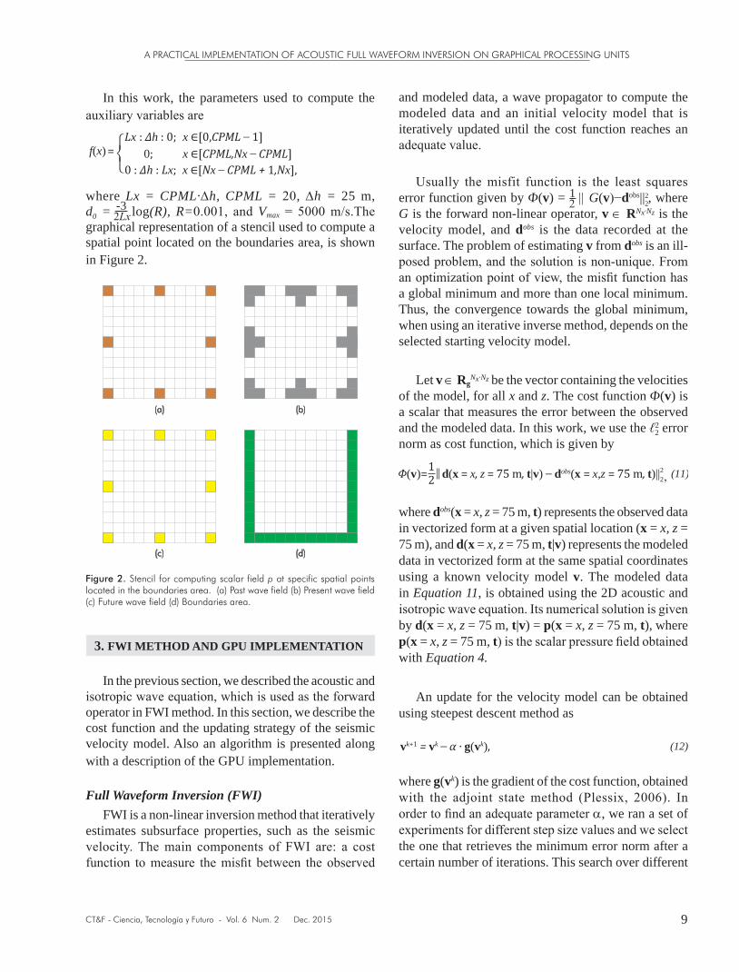
In this work, the parameters used to compute the auxiliary variables are

where Lx = CPML·Dh, CPML = 20, Dh = 25 m, d0 = -3 log(R), R=0.001, and Vmax = 5000 m/s.The graphical representation of a stencil used to compute a spatial point located on the boundaries area, is shown in Figure 2.

3. FWI METHOD AND GPU IMPLEMENTATION

In the previous section, we described the acoustic and isotropic wave equation, which is used as the forward operator in FWI method. In this section, we describe the cost function and the updating strategy of the seismic velocity model. Also an algorithm is presented along with a description of the GPU implementation.

Full Waveform Inversion (FWI)FWI is a non-linear inversion method that iteratively

estimates subsurface properties, such as the seismic velocity. The main components of FWI are: a cost function to measure the misfit between the observed

and modeled data, a wave propagator to compute the modeled data and an initial velocity model that is iteratively updated until the cost function reaches an adequate value.

Usually the misfit function is the least squares error function given by F(v) = 1 || G(v)−dobs||2 2, where G is the forward non-linear operator, v ∈ RNx·Nz is the velocity model, and dobs is the data recorded at the surface. The problem of estimating v from dobs is an ill-posed problem, and the solution is non-unique. From an optimization point of view, the misfit function has a global minimum and more than one local minimum. Thus, the convergence towards the global minimum, when using an iterative inverse method, depends on the selected starting velocity model.

Let v ∈ RgNx·Nz be the vector containing the velocities

of the model, for all x and z. The cost function F(v) is a scalar that measures the error between the observed and the modeled data. In this work, we use the ℓ2

2 error norm as cost function, which is given by

where dobs(x = x, z = 75 m, t) represents the observed data in vectorized form at a given spatial location (x = x, z = 75 m), and d(x = x, z = 75 m, t|v) represents the modeled data in vectorized form at the same spatial coordinates using a known velocity model v. The modeled data in Equation 11, is obtained using the 2D acoustic and isotropic wave equation. Its numerical solution is given by d(x = x, z = 75 m, t|v) = p(x = x, z = 75 m, t), where p(x = x, z = 75 m, t) is the scalar pressure field obtained with Equation 4.

An update for the velocity model can be obtained using steepest descent method as

where g(vk) is the gradient of the cost function, obtained with the adjoint state method (Plessix, 2006). In order to find an adequate parameter a, we ran a set of experiments for different step size values and we select the one that retrieves the minimum error norm after a certain number of iterations. This search over different

(10)f(x) = Lx : ∆h : 0; x ∈[0,CPML _ 1]

0 : ∆h : Lx; x ∈[Nx _ CPML + 1,Nx],0; x ∈[CPML,Nx _ CPML]

(a) (b)

(c) (d)

Figure 2. Stencil for computing scalar field p at specific spatial points located in the boundaries area. (a) Past wave field (b) Present wave field (c) Future wave field (d) Boundaries area.

(11)Φ(v)= d(x = x, z = 75 m, t|v) _ dobs(x = x,z = 75 m, t)||22 12 ,

(12)vk+1 = vk _ α · g(vk),



10

values of a is computationally expensive, and instead this parameter can be estimated using a line-search method, as proposed by Tarantola (1987). The gradient is given by

where the wave field qs is obtained with Equation 4 having as source the error between the modeled and observed data, in reverse time. For this reason, qs is called the back-propagated field of the residual.

Figure 3a shows the propagation of the pressure field generated by a source. Note that the receivers record the pressure wave field at the surface level when a single source is used.

The residual between the modeled and observed seismic traces is then used as a source to find the back- propagated field, qs(x, z, t). This process is shown in Figure 3b. The main difference between Figures 3a and 3b is that in Figure 3b, the original source disappears and each receiver becomes a source whose signature is a residual. The curved lines in Figure 3 illustrate an example of the wavefront propagation of the sources. Having both wavefields, Equation 13 is then used to compute the gradient g(vk).

GPU ImplementationA kernel is a function used to run applications inside

a GPU. When a kernel is launched, it uses blocks with a certain number of threads. A thread represents the minimum group of hardware elements required to run a task. All the threads within the same block work in parallel, and the number of blocks working in parallel depends on the number of streaming multiprocessors (SMs) inside the GPU. Usually, a kernel requires various blocks to execute a function and, depending on the number of SMs, the function is partially or completely parallelized.

We assign Equation 4 to each thread to calculate every future point of the wavefield in parallel (see yellow points in Figures 1, 2 and 3). The total number of future points that can be computed in parallel in the NVIDIA

GeForce GTX 860M are 10240. This occurs since the GPU has 1024 threads per block, two blocks per SMs and five SMs (1024 × 2 × 5, see Table 2). A pseudocode of the implementation is presented in Algorithm 1.

(13)_ ∑ qs(x,z,T _ t) dt, 2 ∂2ps(x,z,t)∂t2g(vk)= (vk(x,z))3

s 0

T

Non−Natural Boundaries

Receiver

Source

Cell Size ∆h=∆x=∆zWave equation propagation

Back propagation

xz

t0

t

Non−Natural Boundaries

Residuals as a source

xz

t

t1

t2

tn

tn

t2

t1

t0

(a)

(b)

Figure 3. (a) Propagation of a source (in red) at different time steps using the wave equation. The receivers are depicted in blue and the boundari-es area is depicted in green. (b) Backpropagation of the residuals (in red) at different time steps using the wave equation. The boundaries area is depicted in green.



4. EXPERIMENTAL RESULTS

In this section, we describe the velocity model and the geometry used to test the FWI implementation. Also, we present the execution time required by our implementation, and the hardware characteristics used in all tests. Furthermore, we present a formulation of the RAM required to perform FWI as well as its experimental validation.

Geophysical ModelThe Marmousi velocity model, created by the Institut

Françãis du Pétrole (IFP) in 1988 (Figure 4a), is used to test the performance of FWI. Particularly, we use a section of this model of 5.25 km × 1.7 km (a grid of 210×68 points with a spatial resolution of 25 m) as depicted in Figure 4b.

The observed and modeled data were produced using

100 sources located at a depth of 75 m. The first source

was placed at 625 m and the final source at 4625 m. The source distribution was computed using

where a is the grid position of the first source (a = 25), b the grid position of the last source (b = 185), n the number of sources (n = 100), SR the spatial resolution (SR = 25 m) and | | represents the operator that takes the nearest integer. The receivers were placed in line on the surface every 25 m, from the position 525 m to the position 4750 m totaling 170. Each receiver recorded 3.5 s at a time step of 4 ms and each source is a Ricker wavelet with a central frequency of 3 Hz. Equation 4 and the Marmousi model (Figure 5a) were used to obtain the observed data. Figure 5b depicts the initial velocity model, v0, which was generated by applying a horizontal recursive smoothing filter to the original model. The filter was recursively applied twenty times using Equation 15, where vn

i,j represents a specific pixel in the velocity model.

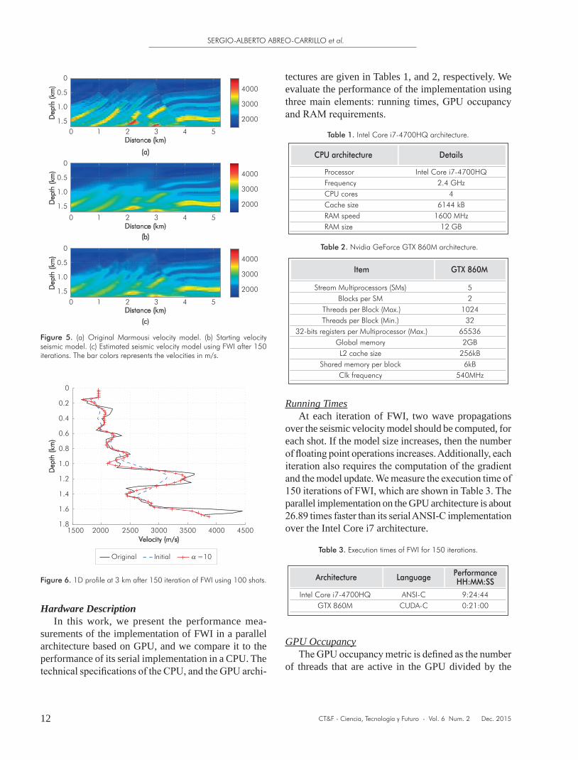
The estimated velocity model after 150 iterations is depicted in Figure 5c. At each iteration, the model is updated using Equation 12, with a = 10. Note in Figure 5c that the low frequency components in the resulting velocity model are correctly estimated. Figure 6 shows a 1D profile of the estimated velocity model. This 1D profile allows for an easy observation of the quality of results.

Algorithm 1 Full Waveform Inversion implemented inside a GPU

1:2:3:4:5:6:7:8:9:10:11:12:

13:14:15:16:17:18:19:20:

21:22:

23:24:25:26:27:28:29:

FWI (v, Obs, s, in f, α)vObssin fαfor i ← 1, iG do acum ← 0 g(x, z) = 0 for j ← 1, Ns do for t ← 1, Nt do

Mod (x,t) ← ps (x,0,t) end for Obsdev ← Obsj,host Residual(x,t) ← Mod (x,t) - Obsdev(x,t) norm←||Residual(x,t)||2

2 acum← 1

2 norma + acum for t ← 1,Nt do

end for

end for φ(i) ← acum v(x,z) ← v(x,z) - α.g(x,z)end forVend ← v(x, z)φ h ← φreturn φ h,vend

FWI inputsStarting velocity model

Observed tracesWavelet source

Location and offset of each shotAlpha value

iG, Number of FWI interations

Ns, Number of sourcesNt, Number of time steps

Observed traces from host to device

(L2 Norm)2

Model update. Equation 12

Final velocity model from device to hostObjective function evolution from device to host

v(x,z)2

1 ∂2ps

∂t2 = + +

∂2ps(x,z,t)∂t2

∂2ps

∂x2∂2ps

∂z2 S(sj,t)

v(x, z)2

1 ∂2qs

∂t2 = + +∂2qs

∂x2∂2qs

∂z2 Residual (x,Nt - t)

g(x, z) = g(x, z) - qs(x,z,T-t) dt(vk(x,z))3

20

T

Equation 13

Distance (km)(a)

(b)

Dep

th (k

m)

0 2 4 6 8 10 122000300040005000

0

1

2

3

Distance (km)

Dep

th (k

m)

0 1 2 3 4 52000

3000

4000

50000

0.5

1.0

1.5

Figure 4. (a) Original Marmousi velocity model. (b) Marmousi trimmed section. The bar colors represents the velocities in m/s.

(14)Sx= SR · ·k a+ k={0, 1, 2,···, n _ 1}(b _ a)(n _ 1)

(15)vi,j = · (vi,j-2 + vi,j-1 + vi,j + vi,j+1 + vi,j+2).n n n n n n15



12

tectures are given in Tables 1, and 2, respectively. We evaluate the performance of the implementation using three main elements: running times, GPU occupancy and RAM requirements.

Running TimesAt each iteration of FWI, two wave propagations

over the seismic velocity model should be computed, for each shot. If the model size increases, then the number of floating point operations increases. Additionally, each iteration also requires the computation of the gradient and the model update. We measure the execution time of 150 iterations of FWI, which are shown in Table 3. The parallel implementation on the GPU architecture is about 26.89 times faster than its serial ANSI-C implementation over the Intel Core i7 architecture.

GPU OccupancyThe GPU occupancy metric is defined as the number

of threads that are active in the GPU divided by the

Hardware DescriptionIn this work, we present the performance mea-

surements of the implementation of FWI in a parallel architecture based on GPU, and we compare it to the performance of its serial implementation in a CPU. The technical specifications of the CPU, and the GPU archi-

Distance (km)

(a)

(b)

(c)

Dep

th (k

m)

0 1 2 3 4 5

0 1 2 3 4 5

0 1 2 3 4 5

2000

3000

4000

0

0.5

1.0

1.5

Distance (km)

Dep

th (k

m)

2000

3000

4000

0

0.5

1.0

1.5

Distance (km)

Dep

th (k

m)

2000

3000

4000

0

0.5

1.0

1.5

Figure 5. (a) Original Marmousi velocity model. (b) Starting velocity seismic model. (c) Estimated seismic velocity model using FWI after 150 iterations. The bar colors represents the velocities in m/s.

Figure 6. 1D profile at 3 km after 150 iteration of FWI using 100 shots.

Velocity (m/s)

Dep

th (k

m)

Original Initial α

1500 2000 2500 3000 3500 4000 4500

0

0.2

0.4

0.6

0.8

1.0

1.2

1.4

1.6

1.8

=10

Table 1. Intel Core i7-4700HQ architecture.

CPU architecture Details

Processor Frequency CPU cores Cache size RAM speed RAM size

Intel Core i7-4700HQ2.4 GHz

46144 kB

1600 MHz12 GB

Item GTX 860M

Stream Multiprocessors (SMs) Blocks per SM

Threads per Block (Max.)Threads per Block (Min.)

32-bits registers per Multiprocessor (Max.)Global memory L2 cache size

Shared memory per block Clk frequency

52

102432

655362GB

256kB6kB

540MHz

Table 2. Nvidia GeForce GTX 860M architecture.

Table 3. Execution times of FWI for 150 iterations.

Architecture Language PerformanceHH:MM:SS

Intel Core i7-4700HQ GTX 860M

ANSI-CCUDA-C

9:24:440:21:00



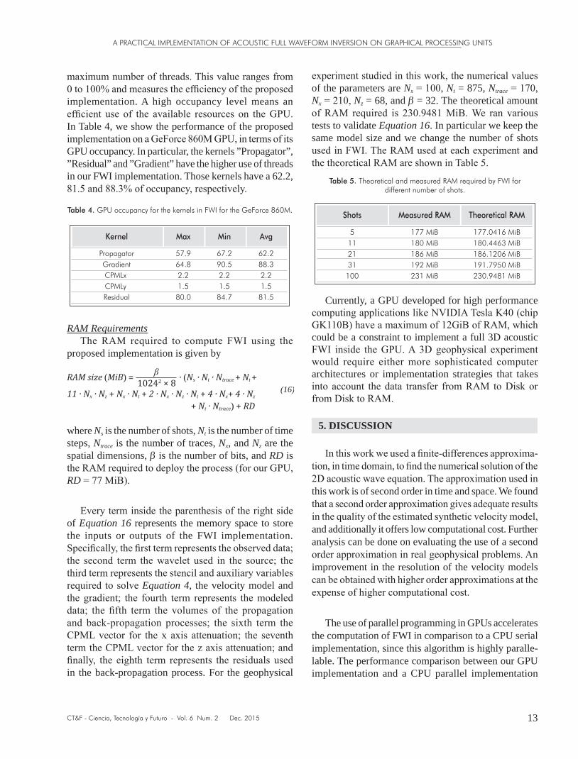
maximum number of threads. This value ranges from 0 to 100% and measures the efficiency of the proposed implementation. A high occupancy level means an efficient use of the available resources on the GPU. In Table 4, we show the performance of the proposed implementation on a GeForce 860M GPU, in terms of its GPU occupancy. In particular, the kernels ”Propagator”, ”Residual” and ”Gradient” have the higher use of threads in our FWI implementation. Those kernels have a 62.2, 81.5 and 88.3% of occupancy, respectively.

RAM RequirementsThe RAM required to compute FWI using the

proposed implementation is given by

where Ns is the number of shots, Nt is the number of time steps, Ntrace is the number of traces, Nx, and Nz are the spatial dimensions, b is the number of bits, and RD is the RAM required to deploy the process (for our GPU, RD = 77 MiB).

Every term inside the parenthesis of the right side of Equation 16 represents the memory space to store the inputs or outputs of the FWI implementation. Specifically, the first term represents the observed data; the second term the wavelet used in the source; the third term represents the stencil and auxiliary variables required to solve Equation 4, the velocity model and the gradient; the fourth term represents the modeled data; the fifth term the volumes of the propagation and back-propagation processes; the sixth term the CPML vector for the x axis attenuation; the seventh term the CPML vector for the z axis attenuation; and finally, the eighth term represents the residuals used in the back-propagation process. For the geophysical

Kernel Max Min Avg

PropagatorGradientCPMLx CPMLy Residual

57.964.82.21.5

80.0

67.290.52.21.5

84.7

62.288.32.21.581.5

experiment studied in this work, the numerical values of the parameters are Ns = 100, Nt = 875, Ntrace = 170, Nx = 210, Nz = 68, and b = 32. The theoretical amount of RAM required is 230.9481 MiB. We ran various tests to validate Equation 16. In particular we keep the same model size and we change the number of shots used in FWI. The RAM used at each experiment and the theoretical RAM are shown in Table 5.

Currently, a GPU developed for high performance computing applications like NVIDIA Tesla K40 (chip GK110B) have a maximum of 12GiB of RAM, which could be a constraint to implement a full 3D acoustic FWI inside the GPU. A 3D geophysical experiment would require either more sophisticated computer architectures or implementation strategies that takes into account the data transfer from RAM to Disk or from Disk to RAM.

5. DISCUSSION

In this work we used a finite-differences approxima-tion, in time domain, to find the numerical solution of the 2D acoustic wave equation. The approximation used in this work is of second order in time and space. We found that a second order approximation gives adequate results in the quality of the estimated synthetic velocity model, and additionally it offers low computational cost. Further analysis can be done on evaluating the use of a second order approximation in real geophysical problems. An improvement in the resolution of the velocity models can be obtained with higher order approximations at the expense of higher computational cost.

The use of parallel programming in GPUs accelerates the computation of FWI in comparison to a CPU serial implementation, since this algorithm is highly paralle-lable. The performance comparison between our GPU implementation and a CPU parallel implementation

Table 4. GPU occupancy for the kernels in FWI for the GeForce 860M.

(16)RAM size (MiB) = · (Ns · Nt · Ntrace + Nt +

β10242 × 8

11 · Nx · Nz + Nx · Nt + 2 · Nx · Nz · Nt + 4 · Nx+ 4 · Nz + Nt · Ntrace) + RD

Shots Measured RAM Theoretical RAM

5112131100

177 MiB180 MiB186 MiB192 MiB231 MiB

177.0416 MiB180.4463 MiB186.1206 MiB191.7950 MiB230.9481 MiB

Table 5. Theoretical and measured RAM required by FWI for different number of shots.



14

remains as on-going research work. One of the main concerns, in the GPU implementation, arises in terms of RAM requirements. For the geophysical experiment studied in this paper, the RAM requirements were satisfied. Nevertheless, real geophysical surveys can require RAM resources larger than 12 GiB. For example, in a 3D FWI, the RAM requirements of our implementation would not be satisfied by current GPU technologies, and FWI implementation should take into account the data transfer between GPU and CPU memories.

Finally, synchronization problems might occur when FWI is computed using parallel architectures such as GPUs. It is critical to implement the algorithm taking into account the synchronization of all the processes running inside the GPU. In the proposed GPU imple-mentation, all points of the future pressure field layer are computed in parallel. Therefore, it is critical to guarantee that present and past pressure field layers are computed before computing the future layer, otherwise an error will be propagated throughout all the layers.

6. CONCLUSIONS

● In this paper, we presented a GPU parallel implemen-tation of the 2D acoustic full waveform inversion. The proposed implementation uses finite-differences in time domain to find the solution of the isotropic and acoustic wave equation. Also, we used the convolu-tional perfect matched layer method to compute the propagated field at the non-natural boundaries. The algorithm uses the adjoint state method to update the velocity models iteratively.

● The proposed parallel implementation was tested for the GPU GTX 860M in terms of running times, RAM requirements and GPU occupancy. Running times were compared to those obtained using serial programming on an Intel Core i7-4700HQ architecture. The high parallelism level of FWI algorithm makes GPU implementation about 26.89 times faster than our sequential implementation. The RAM requirements proposed by Equation 16 were experimentally validated, showing the impact of storing in RAM all the observed data and both wave fields in a 2D FWI. The GPU occupancy presented in Table 4 reveals that none of the kernels uses 100

percent of the resources. This is intrinsic to the propagation process because some kernels are active inside the CPML area and others are active outside the CPML area, but all of them have the same size of the geophysical model (Nx ·Nz).

● In the geophysical experiment the major constraint of the proposed implementation is the memory capacity. Only 230.94 MiB was required for our 2D FWI implementation, for all shot gathers; however a 3D implementation can easily require more than 12 GiB of RAM (the current capacity of a GPU Tesla K40). In that case, a different strategy for implementing FWI should be tested where only one field is stored in RAM, and the other is constantly re-computed. This strategy would use less RAM allowing a 3D implementation.

ACKNOWLEDGEMENTS

This work is supported by Colombian Oil Com-pany Ecopetrol S.A. and Colciencias as a part of the research project grant No. 0266-2013.

REFERENCES

Alford, R., Kelly, K. & Boore, D. M. (1974). Accuracy of finite-difference modeling of the acoustic wave equation. Geophysics, 39(6), 834-842.

Berenger, J. P. (1994). A perfectly matched layer for the absorption of electromagnetic waves. J. Comput. Phy., 114(2), 185-200.

Bunks, C., Saleck, F. M., Zaleski, S. & Chavent, G. (1995). Multiscale seismic waveform inversion. Geophysics, 60(5), 1457-1473.

Cao, D. & Liao, W. (2014). An adjoint-based hybrid compu-tational method for crosswell seismic inversion. Comput. Sci. Eng., 16(6), 60-67.

Collino, F. & Tsogka, C. (2001). Application of the perfectly matched absorbing layer model to the linear elastodynamic problem in anisotropic heterogeneous media. Geophysics, 66(1), 294-307.

Etienne, V., Tonellot, T., Thierry, P., Berthoumieux, V. & Andreolli, C. (2014). Speeding-up FWI by one order



of magnitude. EAGE Workshop on High Performance Computing for Upstream. Chania, Crete.

Hu, W., Abubakar, A. & Habashy, T. M. (2007). Application of the nearly perfectly matched layer in acoustic wave modeling. Geophysics, 72(5), 169-175.

Kim, Y., Shin, C. & Calandra, H. (2012). 3D hybrid waveform inversion with GPU devices. SEG Annual Meeting. Las Vegas, Nevada. SEG-2012-0138.

Lailly, P. (1983). The seismic inverse problem as a sequence of before stack migrations. Conference on Inverse Scattering: Theory and Application. Society for Industrial and Applied Mathematics, Philadelphia, PA.

Mao, J., Wu, R.S. & Wang, B. (2012). Multiscale full waveform inversion using GPU. SEG Annual Meeting. Las Vegas, Nevada, SEG-2012-2575.

Pasalic, D. & McGarry, R. (2010). Convolutional perfectly matched layer for isotropic and anisotropic acoustic wave equations. SEG Annual Meeting. Denver, Colorado, SEG- 2010-2925.

Plessix, R. E. (2006). A review of the adjoint-state method for computing the gradient of a functional with geophysical applications. Geophys. J. Int., 167(2), 495-503.

Tarantola, A. (1984). Inversion of seismic reflection data in the

acoustic approximation. Geophysics, 49(8), 1259-1266.

Tarantola, A. (1987). Inverse problem theory: Methods for data fitting and model parameter estimation. Elsevier.

Thierry, P., Donno, D. & Noble, M. (2014). Fast 2D FWI on a multi and many-cores workstation. EGU General Assembly, 16: Vienna, Austria.

Versteeg, R. & Grau, G. (1991). The Marmousi experience: Proceedings of the 1990 EAEG Workshop on practical aspects of seismic data inversion.

Vigh, D., Cheng, X., Jiao, K., Sun, D. & Kapoor, J. (2014). Multiparameter TTI full waveform inversion on long-offset broadband acquisition: A case of study. SEG Annual Meeting. Denver, Colorado, SEG-2014-0530.

Virieux, J. & Operto, S. (2009). An overview of full-waveform inversion in exploration geophysics. Geophysics, 74(6), 1-26.

Wang, B., Gao, J., Zhang, H. & Zhao,W. (2011). CUDA-based acceleration of full waveform inversion on GPU. SEG Annual Meeting. San Antonio, Texas, SEG-2011-2528.

Weiss, R. M. & Shragge, J. (2013). Solving 3D anisotropic elastic wave equations on parallel GPU devices. Geophysics, 78(2), 7-15.

Yang, P., Gao, J. & Wang, B. (2015). A graphics processing unit implementation of time-domain full-waveform inversion. Geophysics, 80(3), 31-39.

Zhang, M., Sui, Z., Wang, H., Ren, H., Wang, Y. & Meng, X. (2014). An approach of full waveform inversion on GPU clusters and its application on land datasets. 76th EAGE Conference and Exhibition. Amsterdam.

AUTHORS

Sergio-Alberto Abreo-CarrilloAffiliation: Universidad Industrial de SantanderElectronics Engineer, Universidad Distrital Francisco José de CaldasM. Eng. in Electronics Engineering, Universidad Industrial de SantanderPh. D. Student in Electronics Engineering, Universidad Industrial de Santandere-mail: [email protected] Ana-Beatriz Ramírez-SilvaAffiliation: Universidad Industrial de SantanderElectronics Engineer, Universidad Industrial de SantanderM. Sc. in Electronics Engineering, Recinto Universitario de MayaguezPh. D. in Electrical Engineering, University of Delawaree-mail: [email protected]

Oscar ReyesAffiliation: Universidad Industrial de SantanderElectronics Engineer, Universidad Industrial de SantanderM. Eng. in Electronics Engineering, Universidad Industrial de SantanderDr. -Ing. in Computer Science, Hamburg University of Technologye-mail: [email protected]

David-Leonardo Abreo-CarrilloAffiliation: Universidad Industrial de SantanderElectronics Engineer, Universidad Industrial de SantanderM. Eng. Student in Electronics Engineering, Universidad Indus-trial de Santandere-mail: [email protected]



16

Herling González-AlvarezAffiliation: Ecopetrol S.A. - Instituto Colombiano del Petróleo (ICP)Physicist, Universidad Industrial de SantanderM. Sc. in Physics, Universidad Industrial de Santandere-mail: [email protected]

Documents

A PRACTICAL IMPLEMENTATION OF ACOUSTIC FULL WAVEFORM ... · PDF fileA practical implementation of acoustic full waveform inversion on graphical processing units. ... Full waveform