Velocity Analysis ofMulti-Receiver Full Waveform Acoustic

365

Velocity Analysis of Multi-ReceiverFull Waveform Acoustic Logging Data

In Open and Cased Holes

by

Lisa V. Block, C.H. Cheng, and Gregory L. Duckworth

Earth Resources LaboratoryDepartment of Earth, Atmospheric, and Planetary Sciences

Massachusetts Institute of TechnologyCambridge, MA 02139

ABSTRACT

Average semblance and maximum-likelihood spectral analyses are applied to syntheticand field full waveform acoustic logging data to determine formation velocities. Ofparticular interest is the ability of these methods to resolve the P and shear/pseudoRayleigh arrivals in data from poorly-bonded cased boreholes. In synthetic open-holedata the velocity analyses yield results within 4% of the true velocities. Results fromsynthetic well-bonded cased hole data are generally as good as those from the open holedata. However, if the formation P-wave velocity is within roughly 10% of the platevelocity of the steel pipe (about 5.3-5.5 km/s), then there may be a resonance effectthat appears to slow down the P wave slightly (on the order of 6%). For cased-holemodels with no steel/cement bonding (the free-pipe situation), the measured P-wavevelocities are typically 6 to 8% less than the actual formation velocities. If the formationS-wave velocity is greater than about 2.5 km/s, the S-wave velocity estimate may alsobe 6 to 8% low. Furthermore, increasing the thickness of either the cement layer or thefluid layer between the pipe and the cement further decreases the formation velocityestimates. Also, if the P-wave velocity is within roughly 15% of the velocity of the steelarrival, the P wave may not be resolved by the semblance method unless the data isfirst low-pass filtered. Initial tests show that this filtering process may adversely affectthe final P-wave velocity estimate, but the details of this type of approach have notbeen studied. The P wave is resolved. by spectral analysis of the original, nnfiltereddata. For cased-hole models with no cement/formation bonding (the unbonded-casing

366 Block et al.

situation), formation S-wave velocities are estimated to within 3% relative error, andthe formation P-wave velocity is estimated to within 2% error in a slow formation.However, for P-wave velocities between 3.4 km/s and 5.94 km/a, the P wave cannot beresolved by spectral analysis, and it is resolved by the semblance method only in themodel with the low velocity (3.4 km/s).

INTRODUCTION

This paper is a continuation of the work begun last year in velocity analysis of fullwaveform acoustic logging data. Two methods of velocity analysis are employed: themaximum-likelihood method (MLM), which is a high-resolution spectral method, andthe average semblance method. A description of these methods is given in the Appendix. Additional information on the maximum-likelihood method can be found inDuckworth (1983). The objective of this work is two-fold: to determine borehole conditions which allow estimation of formation velocities from full waveform acoustic welllogs, and to compare the performances of the maximum-likelihood method and thesemblance method. Synthetic data sets for open-hole models, well-bonded cased-holemodels, and poorly-bonded cased-hole models are generated using the method of Tubman (1984). (The frequency range of the source function is approximately 4 to 18 kHz.)For each case, models with varying formation velocities are studied. Both velocity analysis techniques are applied to each data set and the results are compared. In this report,the results for the open-hole models and the well-bonded cased-hole models are brieflysummarized. The results for the poorly-bonded cased-hole models are presented in moredetail. These models are divided into two groups: those models in which the steel pipeis not bonded to the cement, referred to as the free-pipe situation, and those models inwhich the cement is not bonded to the formation, referred to as the unbonded-casingsituation. Finally, field data from open and cased holes are analyzed.

RESULTS

Open-hole and Well-bonded Cased-hole Models

Data from open-borehole models have been analyzed for formation P-wave velocitiesof 4.0 km/s, 4.88 km/s, and 5.94 km/s. (The corresponding S-wave velocities are 2.13km/s, 2.6 km/s, and 3.2 km/s.) The P wave and the shear/pseudo-Rayleigh wave areresolved well by both methods. The formation velocities are determined to within 4% ofthe true velocities. The Stoneley wave is resolved by the maximum-likelihood methodat the lowest frequency analyzed, 4 kHz. It is not resolved by the MLM results at higher

Velocity Analysis 367

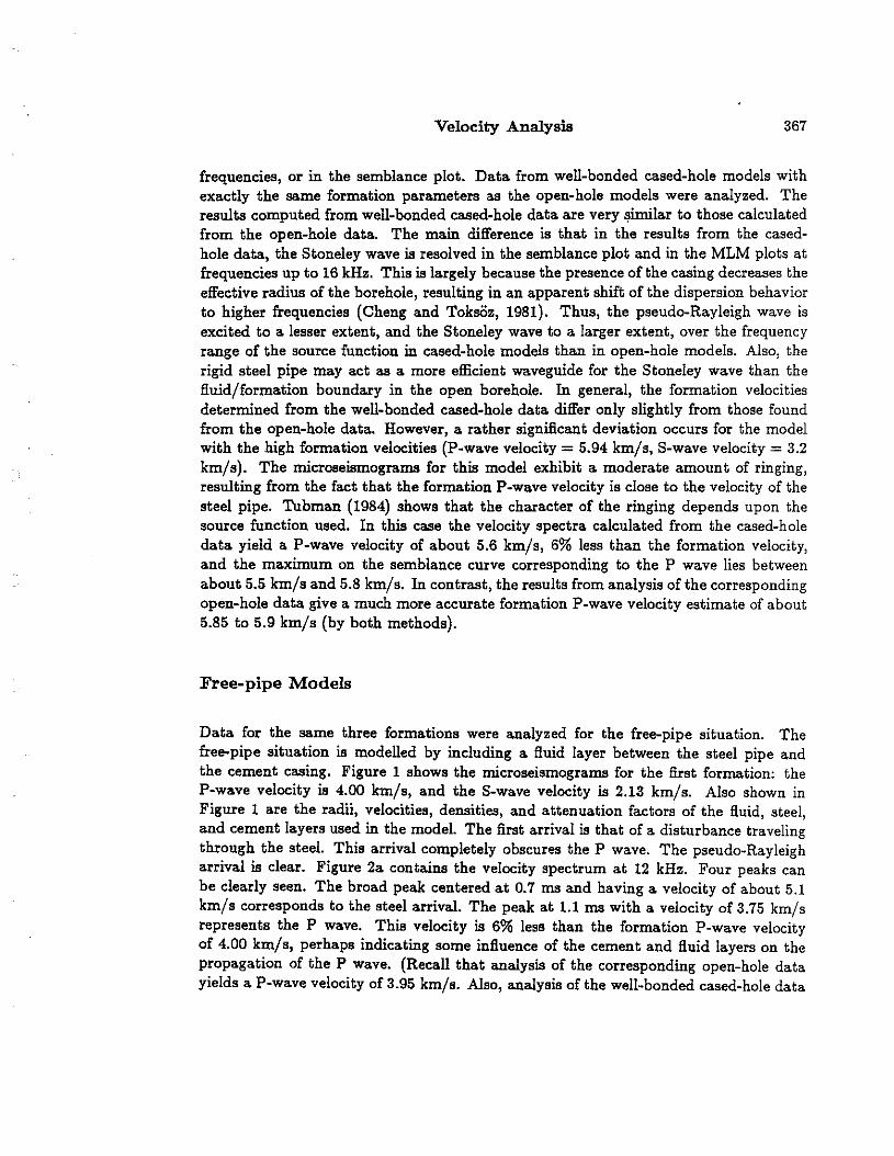
frequencies, or in the semblance plot. Data from well-bonded cased-hole models withexactly the same formation parameters as the open-hole models were analyzed. Theresults computed from well-bonded cased-hole data are very ~imilar to those calculatedfrom the open-hole data. The main difference is that in the results from the casedhole data, the Stoneley wave is resolved in the semblance plot and in the MLM plots atfrequencies up to 16 kHz. This is largely because the presence of the casing decreases theeffective radius of the borehole, resulting in an apparent shift of the dispersion behaviorto higher frequencies (Cheng and Toksiiz, 1981). Thus, the pseudo-Rayleigh wave isexcited to a lesser extent, and the Stoneley wave to a larger extent, over the frequencyrange of the source function in cased-hole models than in open-hole models. Also, therigid steel pipe may act as a more efficient waveguide for the Stoneley wave than thefluid/formation boundary in the open borehole. In general, the formation velocitiesdetermined from the well-bonded cased-hole data differ only slightly from those foundfrom the open-hole data. However, a rather significant deviation occurs for the modelwith the high formation velocities (P-wave velocity = 5.94 km/s, S-wave velocity = 3.2km/s). The microseismograms for this model exhibit a moderate amount of ringing,resulting from the fact that the formation P-wave velocity is close to the velocity of thesteel pipe. Tubman (1984) shows that the character of the ringing depends upon thesource function used. In this case the velocity spectra calculated from the cased-holedata yield a P-wave velocity of about 5.6 km/s, 6% less than the formation velocity,and the maximum on the semblance curve corresponding to the P wave lies betweenabout 5.5 km/s and 5.8 km/s. In contrast, the results from analysis of the correspondingopen-hole data give a much more accurate formation P-wave velocity estimate of about5.85 to 5.9 km/s (by both methods).

Free-pipe Models

Data for the same three formations were analyzed for the free-pipe situation. Thefree-pipe situation is modelled by including a fluid layer between the steel pipe andthe cement casing. Figure 1 shows the microseismograms for the first formation: theP-wave velocity is 4.00 km/s, and the S-wave velocity is 2.13 km/s. Also shown inFigure 1 are the radii, velocities, densities, and attenuation factors of the fluid, steel,and cement layers used in the model. The first arrival is that of a disturbance travelingthrough the steel. This arrival completely obscures the P wave. The pseudo-Rayleigharrival is clear. Figure 2a contains the velocity spectrum at 12 kHz. Four peaks canbe clearly seen. The broad peak centered at 0.7 ms and having a velocity of about 5.1km/s corresponds to the steel arrival. The peak at 1.1 ms with a velocity of 3.75 km/srepresents the P wave. This velocity is 6% less than the formation P-wave velocityof 4.00 km/s, perhaps indicating some influence of the cement and fluid layers on thepropagation of the P wave. (Recall that analysis of the corresponding open-hole datayields a P-wave velocity of 3.95 km/s. Also, analysis of the well-bonded cased-hole data

368

o 1

Block et aL

TIME (ma)

2 3

10

l'

~

4::~... 12I"ilen

""""013

14

15

MODEL PARAMETERS

LAYER OUTER V, V. DENSITY Q, Q,RADIUS (em) (kIn/s) (km/s) (g/ee)

fluid 4.699 1.68 0.00 1.20 20.00 0.00steel 5.715 6.10 3.35 7.50 1000.00 1000.00fluid 6.985 l.68 0.00 1.20 20.00 0.00cement 10.160 2.82 1.73 1.92 40.00 30.00{ormation 00 4.00 2.13 2.16 60.00 60.00

sampling interval = 15.625 fJS

Figure 1: Data for a free-pipe model.

(


o

min = -49, max = -21, inc. = 4

~Me..ured Velocities (km/s):

3.0

VELOCITY (km/s)

l:B-5.0

4.0

2.0

steel 5.1P 3.75pseudo-Rayleigh 2.05

I;S::to:n:.:e:le!..y~ -...:I::.5.:5-"",__-,,_..:::,~ ..L- 2"1.0 '0 2

TIME (ms)

(a)

(b)

2.0 I>

f-;;...ured velOCi~/S): dsteel 5.1 - 5.4P 3.75pseudo-Rayleigh 2.07 9- 7

I;;S:to;:n:,el:;:ey!... .:1.::5.:5_-"'"C-,'1~"'.----'::::. ~-----l1.0 "'0 I 2

TIME (m,)

Figure 2: Velocity analysis of the data in Figure 1. (a) Velocity spectrum at 12 kHz.(b) Semblance.

370 Block et al.

yields a P-wave velocity of about 3.95 to 4.0 km/s.) The pseudo-Rayleigh wave comesin at about 1.6 ms with a velocity of 2.05 km/s, about 3.8% less than the true S-wavevelocity of 2.i3 km/s. (Velocity analysis of the corresponding well-bonded cased-holedata at this frequency yields a velocity estimate of approximately 2.14 km/s. Since thechange in borehole radius due to the casing shifts the dispersion curve of the pseudoRayleigh wave, direct comparison to velocity estimates computed from the open-holedata cannot be made.) The Stoneley wave is represented by the large maximum atabout 2 ms and 1.55 km/s. The semblance is presented in Figure 2b. The steel arrival,P wave, and Stoneley wave appear as strong peaks with the same velocities as in thevelocity spectrum. (The Stoneley arrival is located at 1.8 ms. The linear feature to theleft of the Stoneley wave is due to cycle-skipping 'across the steel arrivaL) The peakrepresenting the pseudo-Rayleigh arrival occurs at a velocity of 2.07 km/s.

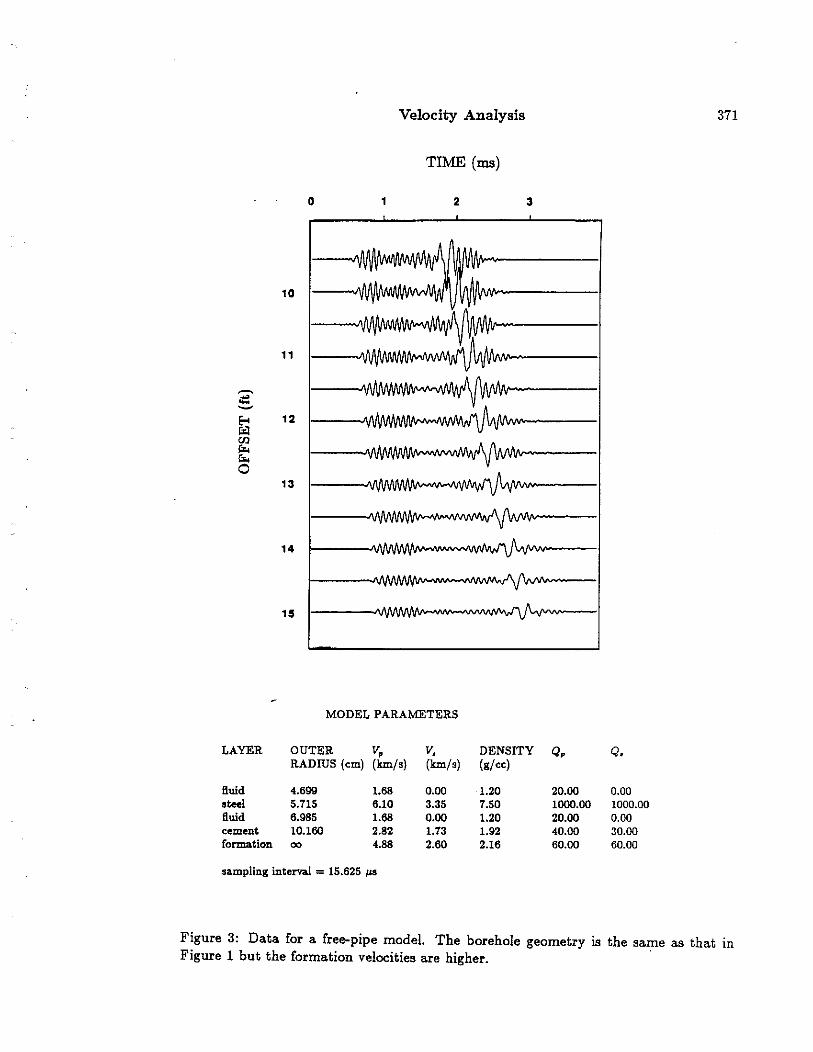
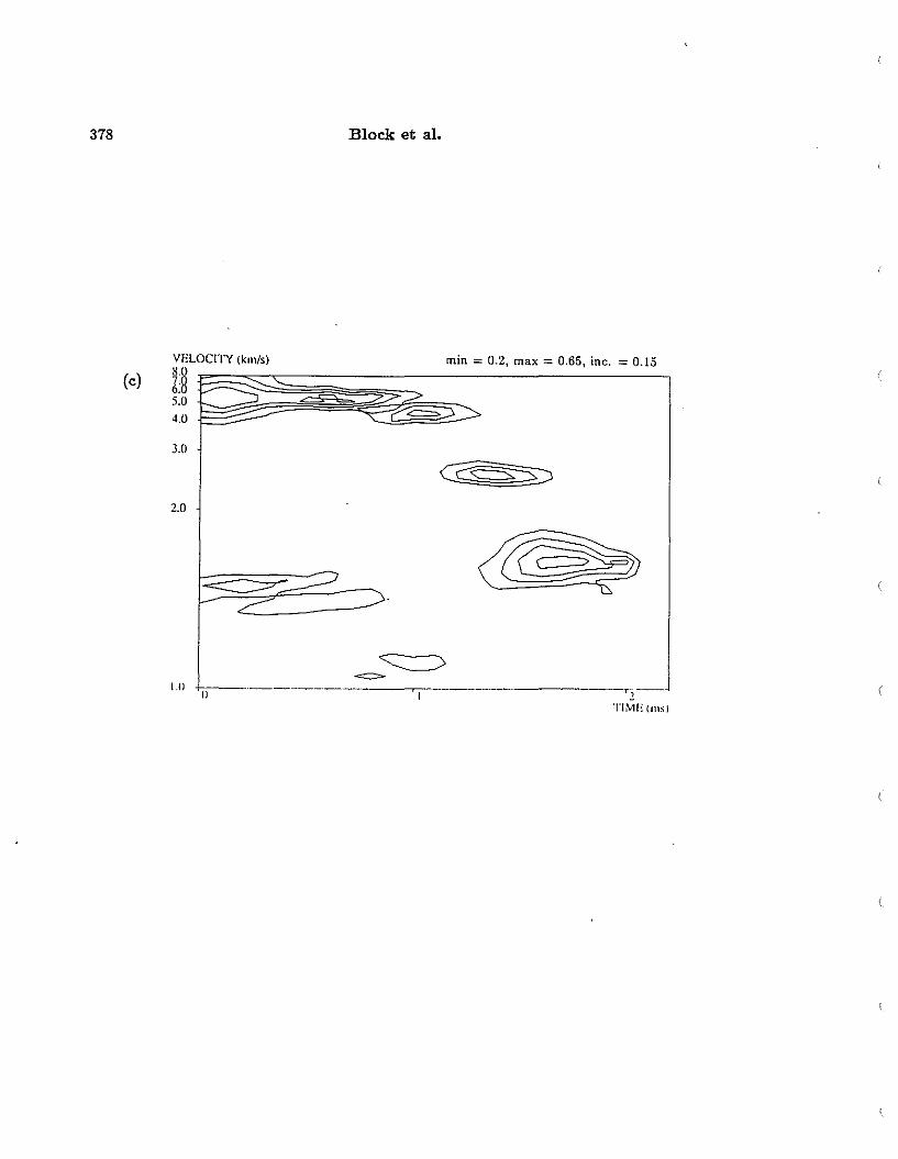
A model having the same geometry as that just discussed but having higher formation velocities is examined. The P-wave velocity for this model is 4.88 km/s, and theS-wave velocity is 2.60 km/s. The data is presented in Figure 3. The duration of thesteel arrival is greater than in the previous model, and therefore the pseudo-Rayleigharrival is not as clear as before. The velocity spectra and semblance are shown in Figures 4a-d. The maximum in the extreme upper left corner of Figure 4a (velocityspectrum at 8 kHz) is due to slight noncausality in the synthetic data. The true steelarrival corresponds to the peak at 0.6 ms and 5.3 km/s. The P wave is represented by asmall peak at 1.05 ms and 4.5 km/s. Again, the measured P-wave velocity is less thanthe formation velocity (by almost 8%). (Analysis of the corresponding open-hole datagives a P-wave velocity estimate of'4.7 to 4.8 km/s, and analysis of the well-bondedcased-hole data yields an estimate of 4.65 km/s.) The steel arrival and P-wave maxima begin to merge with increasing frequency. At 16 kHz (Figure 4c) the steel arrivalis located at 0.8 ms and 5.1 km/s. The P-wave maximum has moved to 1.0 ms andapproximately 4.65 km/s. The pseudo-Rayleigh wave is associated with a distinct peakat a velocity of about 2.45 km/s at all frequencies shown, 6% less than the formationS-wave velocity of 2.60 km/s. The semblance plot in Figure 4d yields the same S-wavevelocity. (Velocity analysis of the corresponding well-bonded cased-hole data yields Swave velocity estimates between 2.52 and 2.65 km/s.) No distinct P-wave maximum ispresent in the semblance results. The steel arrival and the P wave are represented bya linear feature varying in velocity from 4.3 km/s to 5.4 km/s. Apparently the P-waveformation velocity is close enough to the plate velocity of steel to cause minor resolutionproblems in the frequency domain and a total loss of resolution in the time domain. TheStoneley wave maxima occur at a velocity of 1.55 km/s, the same velocity as determinedfor the model with the slower formation velocities. This fact agrees with the observationmade by Tubman et al. (1984) that the casing, rather than the formation velocities, isthe major influence on the Stoneley wave velocity.

Since the P wave is best resolved for the model above in the velocity spectra atthe lower frequencies, an attempt was made to low-pass filter the data and process the

(

o 1

Velocity Analysis

TIME (IDS)

2 3

371

10

11

12

13

14

15

MODEL PARAMETERS

LAYER OUTER Vp V. DENSITY Qp Q.RADIUS (em) (km/.) (km/.) (g/ee)

fluid 4.699 1.68 0.00 1.20 20.00 0.00steel 5.715 6.10 3.35 7.50 1000.00 1000.00fluid 6.985 1.68 0.00 1.20 20.00 0.00cement 10.160 2.82 1.73 1.92 40.00 30.00formation 00 4.88 2.60 2.16 60.00 60.00

sampling interval = 15.625 fJ8

Figure 3: Data for a free-pipe model. The borehole geometry is the same as that inFigure 1 but the formation velocities are higher.

372 Block et al.

min = ~50, max = -18, inc = 4

=

steel 5.3P 4.5pseudo-Rayleigh 2.45Stoneley 1.55

+:0;==:.----.....:..:......-~-4,-4........<:..--.>----'----'--'-....L.12

TIME (ms)

1.0

VELOCITY (km/s)

~:~5.04.0

-M';;;ured Velocities (kmJs):

2.0

3.0

(a)

2TIME (ms)

min = -45, max = -25, inc. = 4

•

5.14.62.451.55

~Measured Velocities (kmJs):

steelppseudo-RayleighStoneleyo

3.0

VELOCITY (km/s)

~:~5.04.0

2.0

1.0

(b)

Figure 4: Velocity analysis of the data in Figure 3. (a) Velocity spectrum at 8 kHz. (b)Velocity spectrum at 12 kHz. (c) Velocity spectrum at 16 kHz. (d) Semblanc·e.


VELOCITY (kmls)

~:~5.0

4.0

3.0

2.0

Measured Velocities (km/s):

min = -40, max = -28, inc = 4

oC)

,teel 5.1P 4.65

.j.~p~,e=u~d~o~-R~a~y~le,=i!!:gh~_...::2.~4~5-L:::"'__-r:- -----l1.0 0 2

TIME (ms)

min = 0.2, max = 0.65, inc. = 0.15VELOCITY (kmls)

(d) ~:~ F~~~~:i~;;-:---l5.0

4.0

3.0

2.0

c__->Measured Velocities (km/s):

steel 4.3 - 5.4pseudo-Rayleigh 2.45Stoneley 1.55

1.0 +0.;-==---------...,.,.------------,"'2-'

TIME (ms)

374 Block et al.

filtered data to see if the P wave could then be resolved by the semblance method. Thefilter shown in Figure 5a was applied to the data to cut off the spectrum between 13and 17 kHz. The filtered data is shown in Figure 5b. The ringing in the data has beenreduced slightly. The results of the semblance are shown in Figure 5c. The P wave isnow represented by a discernable peak at a velocity of about 4.6 km/s, as good as thevelocity estimate obtained via MLM. If the data is filtered to a greater extent, such asshown in Figure 6, the P wave is better resolved in the semblance results. However,the P-wave velocity estimate is reduced. In Figure 6 the spectrum is cut off between11 and 15 kHz, and the P-wave velocity estimate obtained from semblance is about 4.3- 4.35 km/s. (The filtered data and the semblance results for this case are shown inF.igures 6b and c.) In short, a P-wave velocity estimate may be obtained by filteringthe data before applying semblance analysis, but the value of the estimate is sensitiveto the filtering parameters.

For the model with the fast formation (P-wave velocity = 5.94 km/s; S-wave velocity= 3.2 km/s) , a S-wave velocity estimate of about 2.95 km/s is obtained by both methods.This is 8% less the formation S-wave velocity. (Velocities between 3.1 and 3.2 km/s aremeasured in the open-hole situation.) No distinct P-wave maxima are present on theplots. Given the observation that the cement and fluid layers appear to slow down theP wave in the free-pipe situation, the P-wave energy is probably traveling with close tothe velocity of the steel arrival, and hence the P wave is difficult to resolve with thesemethods.

In order to investigate the influence of the cement and fluid layers on the propagationof the P and shear/pseudo-Rayleigh waves, the thickness of the fluid layer was fixed at1.27 cm while the thickness of the cement layer was varied from 3.175 cm to 4.4425cm. Also, the thickness of the cement layer was fixed at 4.4425 cm while the thicknessof the fluid layer was varied from 1.27 cm to 0.025 cm. This procedure was done forthe first two formations above: P-wave velocity = 4.0 km/s (S-wave velocity = 2.13km/s), and P-wave velocity = 4.88 km/s (S-wave velocity = 2.6 km/s). The resultsare summarized in Table 1. From these results it can be concluded that the estimatedvelocity of the P wave decreases as the thickness of either the fluid layer or the cementlayer increases. Furthermore, the higher the P-wave velocity, the greater the absolutechange in the velocity estimate as the geometry varies. Since the formation S-wavevelocities are relatively low, changes in the velocity estimates of the shear or pseudoRayleigh waves with changes in the thicknesses of the fluid and cement layers are notsignificant in these examples. Indeed, the small changes that are observed may mainlybe due to shifts in the dispersion curve of the pseudo-Rayleigh wave with changingeffective borehole radius.

(a)


O.l,2(;;;)()()()=....L.----.J..;-;;Ioooo=------;O';-------+.Ioooo=,.---~---!20000

FREQUENCY (Hz)

TIME (ms)

(b)o 1 2 3

10

11

12

13

14

15

Figure 5: (a) Low-pass filter applied to the free-pipe data in Figure 3. (b) Filtered data.(c) Semblance results for'the filtered data.

376

(c)VELOCITY (km/s)

S'S7.6.5.0

4.0

3.0

2.0

:-

Block et al.

min;;;;;; 0.0, max = 0.6, inc = 0.15

(

I.() +,;,-,-----------....------------c2,--JTIME (ms)

(a)


0·~oooo ·I(XXXI 0 IlXXXI 2000(l

FREQUENCY (Hz)

TIME (ms)

(b) 0 1 2 3

10

11

~.:::~

Eo< 12"=lenr..r..0

13

14

15

•• J\ '.,'v "V IVv'

... I .."V .'" ,IV

... -J ...IV

. . ~\".'\0- I VV

.. \, .I VV

I."V I VV

..'o.J 'V

I \Iv

A"V

Figure 6: (a) Low-pass filter applied to the free-pipe data in Figure 3. (b) Filtered data.(C) Semblance results for the filtered data.

378 Block et al.

min == 0.2, max = 0.65, inc. = 0.15VELOCITY (klll/s)

~:~ ~~~~i"'--'i-~~;;;:~---l~4.0

(cl

3.0

2.0

~-

1.0 0--- .----r;'I-----------ri--TIME tillS)

Velocity Analysis

Formation 1: P-wave velocity = -t.00 km/s, S-wave velocity = 2.19 km/s

Layer Thickness (em] Measured Velocity (km/s)cement fluid P S3.175 1.27 3.75 2.05 2.15

4.4425 1.27 3.5 - 3.6 2.03 - 2.094.4425 0.025 3.75 2.08 - 2.10

Formation 2: P-wave velocity = -t.88 km/s, S-wave velocity = 2.60 km/s

Layer Thickness (ern) Measured Velocity (km/s)cement fluid P S3.175 1.27 4.5 4.65 2.45

4.4425 1.27 4.0 - 4.15 2.42 - 2.454.4425 0.025 4.3 2.45

379

Table 1: Comparison of the thicknesses of the fluid and cement layers ill free-pipesituations and the velocity estimates obtained.

Models with Unhanded Casing

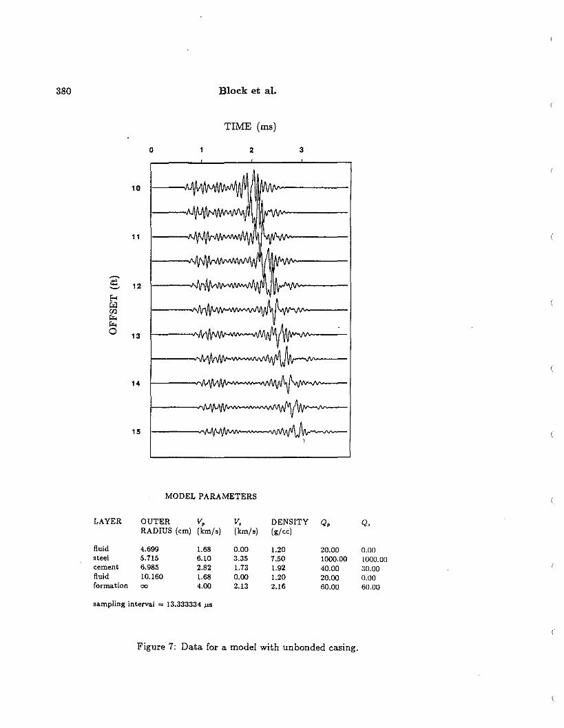
Good steel/cement bonding but no cement/formation bonding, referred to as the unbonded-casing situation, is modelled by inserting a fluid layer between the cement andthe formation. Tubman (1984) showed that if the cement is sufficiently thick (on theorder of 4 ern), it will damp out the casing arrival, and the P-wave arrival can be seen.However, if the cement is too thin, the first arrival on the microseismograms will be dueto a disturbance propagating through the casing with a velocity intermediate betweenthe steel and cement velocities. This situation can be observed in Figure 7. In thismodel, the thickness of the cement is 1.27 ern, and the thickness of the fluid layer is3.18 ern. The complex nature of the first arrival is due to the combined ringing of thesteel and the cement (Tubman, 1984). The amplitude variation within this arrival oftencauses its associated maxima on the velocity spectra to contain several subpeaks. The p_wave arrival is again completely obscured, and the pseudo-Rayleigh arrival is not clear.The formation P-wave velocity for this model is 4.00 km/s, and the S-wave velocity is2.13 km/s. Figures 8a,b contain a typical velocity spectrum and the semblance plot.The maximum representing the pseudo-Rayleigh wave occurs at a velocity of about2.08 km/s on the velocity spectrum and 2.15 km/s on the semblance plot. Hence, a

380 Block et al.

TIME (msJ

o 2 3

10

11

~

it: 12~

l'-<rilenr..r..0 13

14

15

MODEL PARAMETERS

LAYER OUTER V, V. DENSITY Q, Q.RADIUS (em) (km/s) (km/s) (glee)

fluid 4.699 1.68 0.00 1.20 20.00 0.00steel 5.715 6.10 3.35 7.50 1000.00 1000.00cement 6.985 2.82 1.73 1.92 40.00 :10.00fluid 10.160 1.68 0.00 1.20 20.00 0.00formation 00 4.00 2.13 2.16 60.00 60.00

sampling interval = 13.333334 JJS

Figure 7: Data for a model with unbonded casing.

(a)VELOCITY (km/s)8.Ql:tl5.0

4.0

3.0

2.0

Velocity Analysis

min = -38, max = -18, inc. = 5

381

r---o c:;::--Me..ured Velocities (kmjs):

(b)

1.0

3.0

2.0

casingpseudo-Rayleigh

o

4.65 - 4.72.08

TIME (msl

min = 0.25, max::;;; 0.55, inc = 0.1

----::==-~z:_?"':z='>:::J---- .-- ~=----_.Measured Velocities (kmjs):

10

casingplleudo- RayleighStoneleyo

4.65 - 4.72.151.55

2TIME (IUS)

Figure 8: Velocity analysis of the data in Figure 7. (a) Velocity spectrum at 11.7 kHz(b) Semblance

382 Block et al.

good formation S-wave velocity estimate is obtained. The peaks located at a velocityof about 4.65 to 4.7 km/s on the figures correspond to the casing arrival. There is nopeak representing the P wave on either the velocity spectrum or the semblance plot.Apparently these velocity analysis techniques are not powerful enough to separate theP-wave arrival from the complex casing arrival for this model.

Models with lower formation velocities were processed in order to determine whenthe P-wave arrival can be resolved. A model having a formation P-wave velocity of3.7 km/s and a S-wave velocity of 1.97 km/s yielded results very similar to those justexamined. Results for a model having formation P and S-wave velocities of 3.4 km/sand 1.81 km/s, respectively, are presented in Figures 9a and b. The P wave still cannotbe resolved on the velocity spectra, but a weak maximum is present on the semblanceplot between 3.4 and 3.45 km/s. The pseudo-Rayleigh wave is represented by a peak at1.8 km/s on both plots, although on the semblance plot this peak is beginning to mergewith the Stoneley-wave maximum. Finally, data from a slow formation are analyzed.The formation P-wave velocity for this model is 2.9 km/s, and the S-wave velocity is1.52 km/s. A typical velocity spectrum and the semblance plot are shown in Figures lOaand b. A strong peak corresponding to the P wave is seen on the semblance plot, anda smaller maximum occurs on the velocity spectrum. The P-wave velocity measuredfrom these plots is between 2.85 and 2.95 km/s. Hence, an accurate formation P-wavevelocity estimate is obtained for this model. Since the formation S-wave velocity is lessthan the borehole fluid velocity, no shear wave or pseudo-Rayleigh wave is generated.

Unbonded-casing data were also analyzed for the formations with the higher velocities: P-wave velocity = 4.88 km/s (S-wave velocity = 2.6 km/s) and P-wave velocity= 5.94 km/s (S-wave velocity = 3.2 km/s). In each case, the formation S-wave velocitywas estimated to within 3% by both methods, but the P wave could not be resolved byeither method.

The reason why the P wave is more difficult to resolve in the unbonded-casingsituation than in the free-pipe situation is two-fold. First, the casing arrival has a lowervelocity in this situation (4.65-4.7 km/s) than in the free-pipe situation (5.3-5.5 km/s).This casing velocity lies near the center of the P-wave velocity range of interest in welllogging applications - approximately 3.0 to 6.0 km/s. Thus, the casing arrival affectsthe resolution of P waves with moderate to relatively low velocities as well as thosewith high velocities. Secondly, the casing arrival in the unbonded-casing situation ismore complex than the steel arrival in the free pipe situation. This complexity seems tohinder the maximum-likelihood method a little more than the semblance method. In thefree-pipe situation, separate analysis of different frequency components via MLM offersan advantage because the steel arrival and the P wave attain their maximum powerat somewhat different frequencies. In the unbonded-casing situation, this advantageis lost because the addition of the cement layer adds a lower-frequency component tothe casing arrival which apparently overlaps much of the main frequency range of the


(a)VELOCITY (kmls)

l~5.0

4.0

min = -40, max = -25, inc. = 3

casing 4.6

l.;;p::;·e:.:u:.:d:.:o...:-R:::a:::Y.:.le::i~gh::..-_--:1.:.:8 ~I --'-__.L..-__--"I.() T ()

3.0

~Measured Velocitie. (kmj.):

2.0

TIME (ms)

VELOCITY (km/s)

(b) l:~5.0

4.0

min = 0.0, max = 0.6, inc. = 0.1

3.0

2.0

~~~~

Measured Velocitie. (kmj.):~

1.0

steelpp~eudo-Rayleigh

Stoneleyo

4.6 - 4.93.4 - 3.451.81.52

2TIMElms)

Figure 9: Velocity analysis of unbonded-casing data. The borehole geometry is the sameas that shown in Figure 7, but the formation velocities are lower: P-wave velocity = 3.4km/s, S-wave velocity = 1.81 km/s. (a) Velocity spectrum at 12 kHz (b) Semblance

384 Block et al.

<>

min = -55, max = -25, inc. = 5

3.0

2.0

VELOCITY (km/s)8.Qb:tl5.04.0

-c::::= ~<:J-Measured Velocities (kmjs):

casing 4.7 !1.0 g(;~ ----=2:::.9::::5__-..L_..,,---:-_---l---l__.L--.-L'-------'----J

TIME (ms)

(a)

(b)VELOCITY (kmIs) min = 0.2, max = 0.8, inc = 0.15l:S rl?---p----------------,5.0 ~ ~/~4.0

3.0

(

2.0

Meas;':ed VelocitiesTkmjs): ------I.~__-

1.0

casingp

Stoneleyo

4.6 - 4.92.85 - 2.91.52

2TIME(ms)

(

Figure 10: Velocity analysis of data from an unbonded-casing situation in a slow formation. The borehole geometry is the same as that shown in Figure 7, and the formationP and S-wave velocities are 2.9 km/s and 1.52 km/s, respectively. (a) Velocity spectrumat 11.7 kHz (b) Semblance


P wave. When two coherent arrivals with the same frequency and similar slownessesare analyzed by the maximum-likelihood method, the power estimates are biased down.This fact explains why the P wave is not resolved by MLM in most. of the modelsdiscussed above and why the P-wave maximum is very weak in Figure lOa.

Field Data

Figure 11 contains acoustic logging data from an open borehole. Despite the fact thatthe data were recorded in an open borehole, there is a rather large amount of ringing inthe waveforms. The pseudo-Rayleigh wave clearly has a 'multi-pulse' nature, and theP wave appears to consist of two fairly distinct pulses rather than one. Whether thisresponse is due to one or more reflections or whether it is a result of the nature of thetool, or is possibly due to damage around the borehole cannot be determined from thisdata set alone. However, other data sets from the same well exhibit the same behavior,lending support to either of the latter two hypotheses. Velocity spectra at 4.7 kHz and7.8 kHz are presented in Figures 12a and b, respectively, and the semblance is shown inFigure 12c. A P-wave velocity estimate of 6.2 km/s is obtained from Figures 12b andc. (The P wave is not resolved well in Figure 12a because the frequency is low.) Thevelocity spectrum at 4.7 kHz yields a formation S-wave velocity estimate of about 3.22- 3.23 km/s, and the semblance plot gives an estimated velocity of about 3.20 km/s. Inthe velocity spectrum at 7.8 kHz (Fig. 12b), there are two pseudo-Rayleigh wave peaks,one at a velocity of 3.2 km/s and one at a lower velocity of around 2.85 km/s. It is not \clear whether these two peaks represent two pseudo-Rayleigh modes, or whether theyare simply a result of the complex nature of the waveforms described above.

Figure 13 contains microseismograms from the same well as above, and from thesame depth, but after the well was cased. The casing is well-bonded in this part of thewell, and thus the first arrival is the P wave. Figure 14a shows the velocity spectrum at7.8 kHz, and Figure 14b contains the semblance plot. The P wave is represented by amaximum at a phase velocity of 6.3 km/s in the velocity spectrum, and 6.1 km/s in thesemblance plot. These results are consistent with those from the open-hole log. In thevelocity spectrum at 7.8 kHz, the pseudo-Rayleigh wave is represented by several peaksvarying in velocity from about 3.0 to 3.5 km/s. The small peak at a time of 2.85 ms anda velocity of 2.95 km/s is believed to represent the Airy phase of the pseudo-Rayleighwave. The overall increase in the pseudo-Rayleigh wave velocity is consistent withthe theory that the pseudo-Rayleigh wave dispersion curve shifts to higher frequencieswhen the effective borehole radius decreases due to the casing (Cheng and Toksiiz,1981). Also, this shift of the dispersion curve explains why the pseudo-Rayleigh waveis not resolved in the velocity spectrum at 4.7 kHz for the cased-hole data (not shown).In the semblance plot, the pseudo-Rayleigh wave peak exhibits dispersion, varying invelocity from about 3.15 to 3.4 km/s. The smaller subpeak to the right (centered at

386 Block et al.

TIME (ms)

2 3 4

10

11

12

13

Figure 11: Field data from an open borehole.



]

TIME (illS)

omin = -20, max::::::; 24, inc. ::::::; 4

2

3.22 - 3.231.52

pseudo-RayleighStoneley

3.0

2.0

VELOCITY (km/s)8.Ql:ti5.0

4.0

1.0

(a)

.lTIME (ms)

oo6.2

2.85 & 3.21.55


p

pseudo-RayleighStoneJey

3.0

VELOCITY (km/s) min ::::::; -13, max = 23, inc_ ::::::; 4.ts ~~TTT"rIT--;r--r-'-~--'--~1l5.0

4.0

2.0

1.0

(b)

Figure 12: Velocity analysis of the data in Figure 11. (a) Velocity spectrum at 4.7 kHz(b) Velocity spectrum at 7.8 kHz (c) Semblance

388 Block et al.

min = 0.2, max = 0.8, inc. = 0.1

3.0

2.0

VELOCITY (km/s)

l:8 ~~~----:C~c=5F'~~>l5.0~~~~~~4.0

(c)

MeasuredVelocities (km/s);:::>~

1.0

p

pseudo-RayleighStoneley

6.23.21.55

2 3TIME (illS)

(

about 2.7 ms) represents the Airy phase and yields a velocity of 3.0 km/s. Recall thatno dispersion was noticed in the semblance plot for the open-hole data (Figure 12c).This suggests that the higher frequencies of the pseudo-Rayleigh wave are being excitedto a greater degree in the cased hole than in the open hole. This hypothesis could alsoexplain why the Stoneley wave is resolved in the velocity spectrum at 7.8 kHz for theopen-hole data but not for the cased-hole data. According to this idea, the pseudoRayleigh wave is excited to a greater degree at 7.8 kHz in the cased hole than in theopen hole, making the Stoneley wave more difficult to resolve.

The data shown in Figure 15 was recorded in the same well as the previous databut in a different formation. These traces are from the open-hole log. Although thedata is noisy, the P wave, the pseudo-Rayleigh wave, and the Stoneley wave can bedistinguished. The velocity spectra at 4.7 and 7.8 kHz are presented in Figures 16aand b, and the semblance plot is shown in Figure 16c. The P-wave velocity estimatevaries from plot to plot. The velocity spectrum at 4.7 kHz yields an estimate of 5.3 5.35 km/s, the spectrum at 7.8 kHz gives a velocity of 5.6 - 5.7 km/s, and from thesemblance plot an estimate of about 5.5 km/s is obtained. The values of the formationS-wave velocity estimate range from 2.87 km/s to 3.03 km/s. As in the other data sets,two pseudo-Rayleigh peaks are observed in the velocity spectrum at 7.8 kHz.

Velocity Analysis

TIME (IDS)

389

1 2 3 4

10

11

12

13

Figure 13: Field data from a well-bonded cased hole. The data is from the same welland the same depth as the data shown in Figure II.

390 Block et al.


3TIME (ms)

•

min = -3, max:::; 29, inc. = 4

o6

2

<::>

6.3

3.052.95

p

pseudo-RayleighAiry ph~ of pR

2.0

VELOCITY (kmfs)8.Q6:ti5.0

4.0

3.0

1.0

(a)

min = 0.15, max::; 0.675, inc. :;::; 0.075(b)

VELOCITY (kmfs)

UF~=~--l::: <?:~~===s.

2.0

Measured Velocities (km/s):o

1.0

p

pseudo-RayleighAiry ph""e of pitStandey

6.1~

3.15 - 3.4 >3.01.52


Velocity Analysis

TIME (ms)

391

1 2 3 4

10

11

12

13

Figure 15: Field data from an open borehole.

392 Block et al.

Measured Velocitie, (krn/,):

3TIME (illS)

min = -15, max == 29, inc. == 4

2

5.3 - 5.352.95(1.40

ppseudo-RayleighStoneley

2.0

VELOCITY (Ian/,)8.Ql:tl5.0

4.0

3.0

1.0

(al

min == -8, max == 22, inc. = 3

G<:)

o~Measured Velocities (krn/,):

3.0

VELOCITY (km/,)

8.~7.6.5.0

4.0

2.0

(b)

1.0

p

p~eudo-Rayleigh

Stoneley

5.6 - 5.72.87 & 3.031.15

2 .1TIME (illS)

Figure 16: Velocity analysis of the data in Figure 15. (a) Velocity spectrum at 4.7 kHz(b) Velocity spectrum at 7.8 kHz (cl Semblance


Measured Velocities (kmjs):

3.0

2.0

VELOCITY (km/s) min = 0.2, max = 0.8, inc. = 0.075

l:~ ~~~-------I5.0 ~=~...~~.. :::J)4.0

(c)

ltl

ppseudo-Ra)'JeighStoneley

5.52.951.47

.1TIME(ms)

The microseismograms in Figure 17 are from the cased-hole log, at the same depth asthe data just examined. The hole was not cemented at this depth - the steel pipe is notbonded to the surrounding rock. Hence, this data corresponds to a special case of thefree-pipe situation. Figures 18a and b contain the velocity spectrum at 7.8 kHz and thesemblance contour plot, respectively. Five arrivals are resolved on the velocity spectrum:the Stoneley wave at a velocity of about 1.53 km/s, the shear/pseudo-Rayleigh arrivalat a velocity of 2.9 to 2.95 km/s, the Airy phase of the pseudo-Rayleigh wave at avelocity of 2.6 km/s, and two arrivals at relatively high velocities of approximately 5.0km/s and 5.5 - 5.6 km/s. From analysis of the open hole data, the P wave is expectedto have a velocity between 5.3 and 5.7 km/s. The steel arrival, however, also travelswith a velocity in this range, and hence it is impossible to determine which maximumcorresponds to the P wave and which one corresponds to the steel arrival. In practice,continuity of the peaks over a range of depths would be needed to correctly identify thetwo arrivals. On the semblance plot (Figure 18b) there is only one high-velocity arrival(at 5.5 km/s). This lack of resolution in the semblance results is consistent with earlieranalysis of synthetic data (Recall Figure 4d). Maxima representing the shear/pseudoRayleigh wave and the Stoneley wave are present in the semblance results. However,these maxima are not prominent due to the large amount of interference from thesteel arrival. The S-wave velocity estimated from this plot is 2.7 km/s. This data setwas low-pass filtered several times to attempt to improve the semblance results. The

394 Block et al.

TIME (ms)

2 3 4

10

11

~

.;::~

Eo<

""en...... 120

13

Figure 17: Field data recorded in a borehole with a 'free pipe'. This data is from thesame well and the same depth as the data shown in Figure 15.


(a)VELOCITY (km!s)

l:85.0~~~~

4.0

min = ~4, max = 28, inc. = 4

3TIME (ms)

9

o

2

5.0 & 5.5 - 5.62.9 - 2.952.61.53

Steel &< Ppseudo-RayleighAiry phase or pRSloneley


2.0

3.0

1.0

min = 0.15, max = 0.825, inc. = 0.075


3.0

VELOCITY (krn!s)

l:8 ,~~=------:..£.~~>50~ ~4.0

2.0

(b)

1.0

steellPpseudo-RayleighAiry phase of pRStondey

5.52.72.651.55 - 1.65

2 3TIME (illS)


396 Block et al.

filtering greatly enhanced the overall quality of the semblance plots, but two distincthigh-velocity events (Le., the P wave and the steel arrival) could not be resolved in anyof the results. One of the filters used is shown in Figure 19a, and the correspondingfiltered traces are presented in Figure 19b. The results of applying the semblancemethod to this filtered data are shown in Fig. 19c.

CONCLUSIONS

The average semblance and the maximum-likelihood spectral analysis yield good resultsfor synthetic open-hole data. The estimated formation velocities vary by not more than4% from the true velocities. For synthetic data from well-bonded cased boreholes, theresults are generally about the same as for open holes. However, for very fast formations(having a P-wave velocity close to that of the steel pipe), there may be a resonance effectthat appears to slow down the P wave slightly.

The major conclusions from analysis of data from poorly-bonded cased-hole modelsare summarized in Table 2. For cased-hole models with no steel/cement bonding (thefree-pipe situation), the measured formation P-wave velocities are approximately 6 to8% less than the actual velocities. Thus, the greater the formation P-wave velocity,the poorer the velocity estimate. Also, if the formation S-wave velocity is relativelyhigh (about 2.5 km/s or greater), then the S-wave velocity estimate may also be onthe order of 8% low. This decrease in the measured velocities is apparently due to theinfluence of the cement and fluid layers on the propagation of the P and shear/pseudoRayleigh waves. The velocity estimates become even worse when the thickness of thefluid layer or the cement layer is increased. Thus, variations in the thickness of thecement layer and/or the fluid layer in the free pipe situation may produce perturbationsin the velocity log which are not related to any change in the character of the formation.Furthermore, when the formation P-wave velocity is relatively close to the steel velocity(within roughly 15%), the P-wave arrival cannot be separated from the steel arrivalby applying the semblance method to the raw data. The two arrivals are resolved byspectral analysis, although the quality of resolution may vary with frequency. Initialtests show that the P wave may be resolved by the semblance method for this situationif the data is first low-pass filtered. However, the resulting velocity estimate is affectedby the filtering process. Further details of this approach have not been pursued in thisstudy.

For cased-hole models with no cement/formation bonding (the unbonded-casing situation), neither velocity analysis method can resolve the P-wave arrival when the Pwave velocity differs from the velocity of the casing arrival by less than about 28%. Thesemblance method gives better results than MLM in marginal cases. For example, forthe casing parameters used in these studies, the casing arrival has a velocity of 4.65

(a)

Velocity Analysis

() ·20()OO -J(KKKI 0 J(KKXI 2(XI()O

FREQUENCY (Hz)

TIME (ms)(b)

2 3 4

397

10

11

12

13

Figure 19: (a) Low-pass filter applied to the data in Figure 17. (b) Filtered data. (c)Semblance results from the filtered data.

398 Block et al.

-='"2.0

VELOCITY (km/s) min:;;;; 0.15, max = 0.75, inc. = 0.075

l:S~I~~~=--=~-'l5.0

4.0

3.0 ~J5i ~-2?

k"J~~v

(c)

1.02

km/s. For models with P-wave velocities ranging from 3.4 km/s to 5.94 km/s, the Pwave cannot be resolved by the maximum-likelihood method. This arrival is resolved bythe semblance method only for the model with the P-wave velocity of 3.4 km/s. (Thecorrect velocity of 3.4 km/s is obtained.) For all of these models, the formation S-wavevelocity is determined by both methods to within 3% relative error. Also, for a slowformation (P-wave velocity = 2.9 km/s), the formation P-wave velocity is estimated towithin 2% error by both methods. The inability of either method to resolve the P waveover a large range of velocities greatly reduces the usefulness of data recorded in holeswith unbonded casing.

Although not presented in this report, models having fewer receivers (as few as four)and a larger receiver spacing (1.0 ft.) were analyzed. When the number of receiversis decreased, the peaks corresponding to the casing, P, pseudo-Rayleigh, and Stoneleyarrivals are still present. However, the velocity resolution is decreased, and the aliasingpeaks on the MLM plots are increased in amplitude. In some cases the aliasing peaksare about as strong as the main peaks. When the receiver spacing is increased from 0.5ft. to 1.0 ft., the main peaks can still be identified, but the number of aliasing peaks onthe MLM plots and the number of cycle-skipping peaks on the semblance plot increase.

The field data which has been analyzed thus far supports the results found from


Formation Free-pipe Unbonded-CasingVelocities MLM Semblance MLM SemblanceVery Slow (no OK * OK * OK I OKS-wave)

Slow OK * OK * cannot sep- weak but dis-arate P wave tinguishable P-from casing ar- waverival maXImum

Moderate OK OK cannot sepa- cannot sep-rate P-wave arate P wavefrom casing ar- from casing ar-rival rival

Fast OK filtering re- cannot sep- cannot sep-quired to sepa- arate P wave arate P waverate P-wave from casing ar- from casing ar-from casing arrival rivalrival

Very Fast (P- cannot sep- cannot sep- cannot sep- cannot sep-wave vel. "'" 6 arate P wave arate P wave arate P wave arate P wavekm/s) from casing ar- from casing ar- from casing ar- from casing ar-

rival rival rival rival

Table 2: Summary of the major conclusions from analysis of synthetic acoustic loggingdata for free-pipe and unbonded-casing situations. The * denotes situations that werenot modelled - these conclusions were deduced from the other results.

the study of the synthetic data. The maximum-likelihood method and the semblancemethod generally work well in data from open holes and well-bonded cased holes. Themaximum-likelihood method has been found to yield better results than the semblancemethod on data recorded in a free pipe in a formation having a P-wave velocity ofabout 5.5 km/s. In other free pipe situations, in formations having lower velocities,both methods have been found to work equally well. No data recorded in a well withunbonded casing has yet been analyzed.

400 Block et al.

ACKNOWLEDGEMENTS

This work was supported by the Full Waveform Acoustic Logging Consortium at M.LT.Lisa Block .was also supported by the Phillips Petroleum Fellowship.

REFERENCES

Cheng, C. H., and Toksoz, M. N., 1981, Elastic wave propagation in a fluid-filled boreholeand synthetic acoustic logs; Geophysics, 46, 1042-1053.

Duckworth, G. L., 1983, Processing and inversion of Arctic Ocean refraction data; Sc.D.thesis, Joint Program in Ocean Engineering, Mass. Inst. Tech., Cambridge, Massachusetts, and Woods Hole Oceanographic Institution, Woods Hole, Massachusetts.

Tubman, K. M., 1984, Full waveform acoustic logs in radially layered boreholes: Ph.D.thesis, Mass. Inst. Tech., Cambridge, Massachusetts.

Tubman, K. M., Cheng, C. H., and Toksoz, M. N., 1984, Synthetic full waveform acousticlogs in cased boreholes; Geophysics, 49, 1051-1059.

APPENDIX - VELOCITY ANALYSIS

Windowing the Data

The velocity analyses are implemented within short time windows of given moveoutacross the receiver array. An example of such a window is shown in Figure A - 20. r isthe beginning time of the window on the near trace, T is the length of the window, and vis the slope (dxldt) of the window. v is equal to a trial phase velocity in the direction ofthe array. For receivers in a borehole, the signals travel essentially parallel to the array,and hence v is equal to the phase velocity of propagation. (The paths taken from thetool to the borehole wall and vice versa require about the same amoun t of time for eachreceiver and hence do not significantly affect the moveout of the signaL) For a fixed timer, calculations are made for many different slownesses. The window is then advanced bya small amount, dr. and the process is repeated. The final result is a series of contourplots. Each plot is a function of time r and velocity v. One plot is obtained from thesemblance method and several plots are obtained from the maximum-likelihood method,each at a fixed frequency. As will be seen below, the output of the maximum-likelihood

(

(

(


~

~~ 12

""'ril

'"......0

13

1

10

11

14

15

o

TIME (ms)

2

t --->

3

v = dxldt = lip

Figure A - 20: Window Parameters

402 Block et al.

Semblanceavg (r, v= ~) =

method is proportional to slowness p, rather than velocity. To maintain equal resolutionacross the contour plots, the calculations are made at equal increments of p, and so thevelocity axis is linear in slowness.

Average Semblance

The average semblance is the ratio of the energy of a stacked trace to the sum of theenergies of the individual traces within a time window, divided by the number of traces.Let x (t, Zk) represent the time series at distance Zk. Then the average semblance withinthe time window at position r with moveout v (Recall Figure A - 20) is given by:

,+pz.+T (N-l )2"~~PZ' ~ X (to, Zk)

T+pZk+T N-l

N I: I: (x (to, Zk))2t,l;=T+pZk k=O

The values of average semblance range from zero to one.

The Maximum-Likelihood Method

This method essentially consists of computing a two-dimensional Fourier transformwithin the time window. The output is power, contoured in dB. Let x (t, Zk) represent the time series at distance Zk, as defined previously. For simplicity, the near tracein the data set is taken to be at distance 0, i.e., ZQ = o. An estimate of the temporalFourier transform of the data within the time window illustrated in Figure A - 20, forthe receiver located at distance Zk, is given by:

('+TX(r,w,zk)=e-;wz,p J, X(t+Zkp,Zk) w(t-r) e;W'dt.

Recall that r is the beginning time of the window on the near trace, T is the length ofthe window in time, and p is the slowness associated with the moveout of the windowacross the traces. Since a shift in the time domain corresponds to multiplication by acomplex exponential in the frequency domain, the term in front of the integral must beincluded to restore the proper phase to the spectrum. w (t) is a window function whichis used to improve the resolution of the estimated spectrum. The estimated spectrum isthe true frequency spectrum of the data within the short time window convolved withthe frequency spectrum of the window function. (This distortion is the 'smearing' ofthe frequency spectra which is referred to in the text.) The window function used inthis study is sin2 (if). In practice, this integral must be converted into a summation


(i.e., a discrete Fourier transform or DFT). The Fourier coefficients for all frequencies(up to the Nyquist frequency) are computed simultaneously using an FFT algorithm.

At a fixed frequency, wo , an estimate of the spacial transform may be obtained bysumming across the receivers as follows:

N-l

X ( p) '" X ( w z) e-iw<>PZk lizr,wo, = L.. a. r, 0, •

• =0

where N is the number of receivers in the array and liz is the receiver spacing. Sincewavenumber k is equal to WoP, with Wo fixed, the transform has been written as afunction of slowness p rather than wavenumber. The a. are 'weights' on the receiverswhich perform the same function in the spacial transform that the window functionw(t) performs in the temporal transform. The estimated spacial transform, X (r, wo, p),is the actual transform. of the data convolved with the spacial transform of the weightfunction (ao, ai, ... ,aN-I). In conventional spectral analysis, also called beamforming,these weights are fixed while the Fourier coefficients are computed for all wavenumbers,or slownesses, of interest. In the maximum-likelihood method, however, a new setof weights is determined for each slowness considered. This procedure improves theresolution of the final velocity spectrum, since it decreases interference from componentstraveling with nearby slownesses. The way in which the a. are determined will beaddressed shortly. The previous equation may be rewritten in vector form as:

X(r,wo,p) = A' X

where

A=

aoeiwopzo 8z

aleiwoPZl 8z

X=

X (r, wo, zo)X (r, W o , Zl)

aN_leiwoPZN-l liz X (r w z ), 0, N-l

and * denotes complex conjugate transpose. The estimate of the power due to the planewave component traveling with slowness p at frequency W o is:

p. (r,wo,p) = II X(r,wo,p) 112

= II A' X 112

= A' Kx

AT T ----

h K ( XX·). t' t d I' .were -2S. = -r IS an es tma e spectra covarIance matrIX.

In order to determine the optimum weights (a.), two issues must be considered.First, when a certain slowness p is being scanned, it is required that the contributionto the power estimate due to a plane wave component propagating with that slownessbe unbiased. To state this mathematically, let Be'woP'. represent the temporal Fourier

404 Block et al.

II A' BE 11 2 B 2

T =1'

transform (at frequency wo) of the plane wave component of interest at receiver k.we require that:

Then

where

E=

eiWoPZN_l

This reduces to:A' E = 1.

Another way to think about this constraint is that we are requiring the spacial transformof the weight function (ao,al, ... ,aN-tl to have a value of 1 at p = o. Thus, when thistransform is convolved with the spacial transform of the plane wave component at p, avalue of B will be obtained as required. Although the contribution to the power estimatefrom the plane wave component with slowness p is unbiased, the total power estimatemay still be wrong due to 'contamination' from components with nearby slownesses. Toreduce this problem, the total power estimate is minimized:

min (A' K x AJ .

Hence, we wish to minimize the total power estimate, A' K x A, subject to the constraintA' E = 1. Using the Lagrange multiplier method, it can be shown that the matrix Awhich satisfies these requirements is given by:

K -1 EA- x-- E' K 1 E·

- ---A -

Substituting this result into the expression for the power estimate yields:

To summarize the procedure, for a fixed window position, (T, p), an FFT is performedon each trace to yield all of the frequency coefficients at one time. A spectral covariancematrix is then formed for each frequency of interest. The power estimate is computedvia the above formula for each frequency. This procedure is repeated for each newwindow position. The final result is a series of contour plots. Each plot is a function ofT and p at a fixed frequency.

Documents

Velocity Analysis ofMulti-Receiver Full Waveform Acoustic