SLIMUniversity  of  British  Columbia

Tristan  van  Leeuwen,  University  of  British  ColumbiaSasha  Aravkin,  Michael  Friedlander  &  Felix  Herrmann

Recent advances in seismic waveform inversion

ICME  Comp.  Geosciences  Seminar,  Stanford,  01-­‐10-­‐2012

SLIM

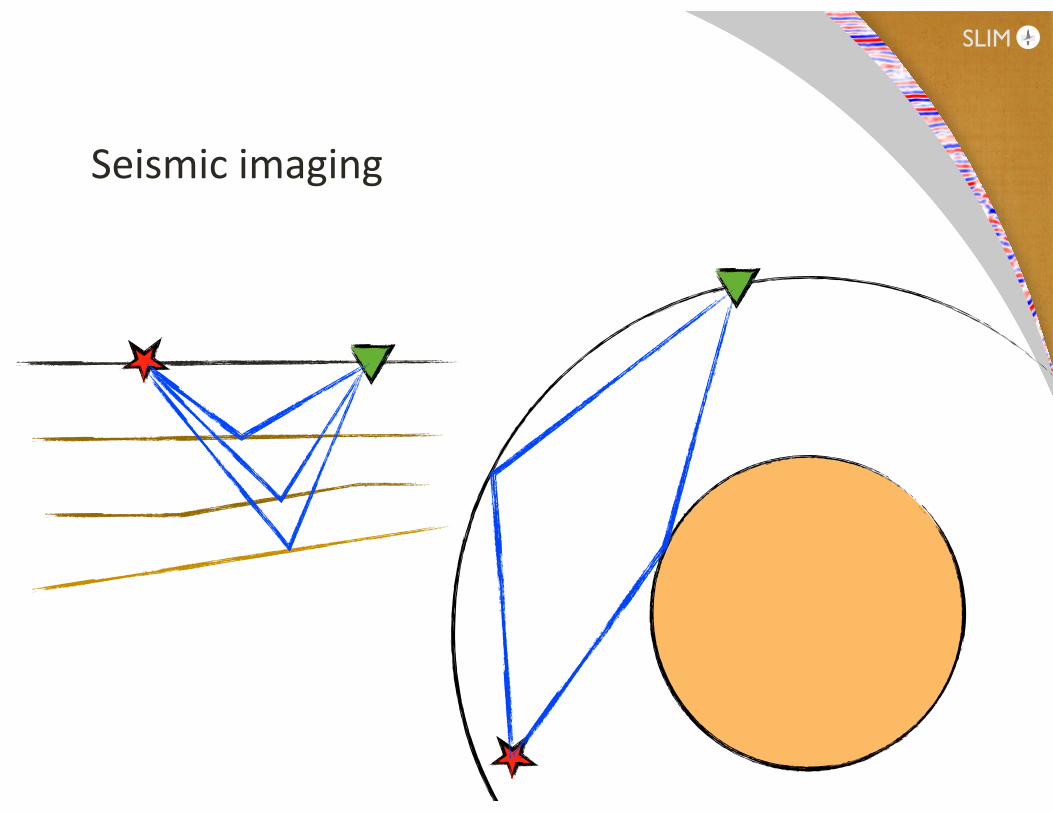
Seismic  imaging

SLIM

SLIM

offset [m]

time

[s]

0 200 400 600

0

0.5

1

1.5

2

2.5

3

3.5

4

offset [m]

time

[s]

0 200 400 600

0

0.5

1

1.5

2

2.5

3

3.5

4

offset [m]

time

[s]

0 200 400 600

0

0.5

1

1.5

2

2.5

3

3.5

4

shot pos. [m]

time

[s]

0 200 400 600

0

0.5

1

1.5

2

2.5

3

3.5

4

SLIM

• Full  waveform  inversion• General  formulation• Nuisance  parameters• Fast  optimization• Summary

Overview

SLIM

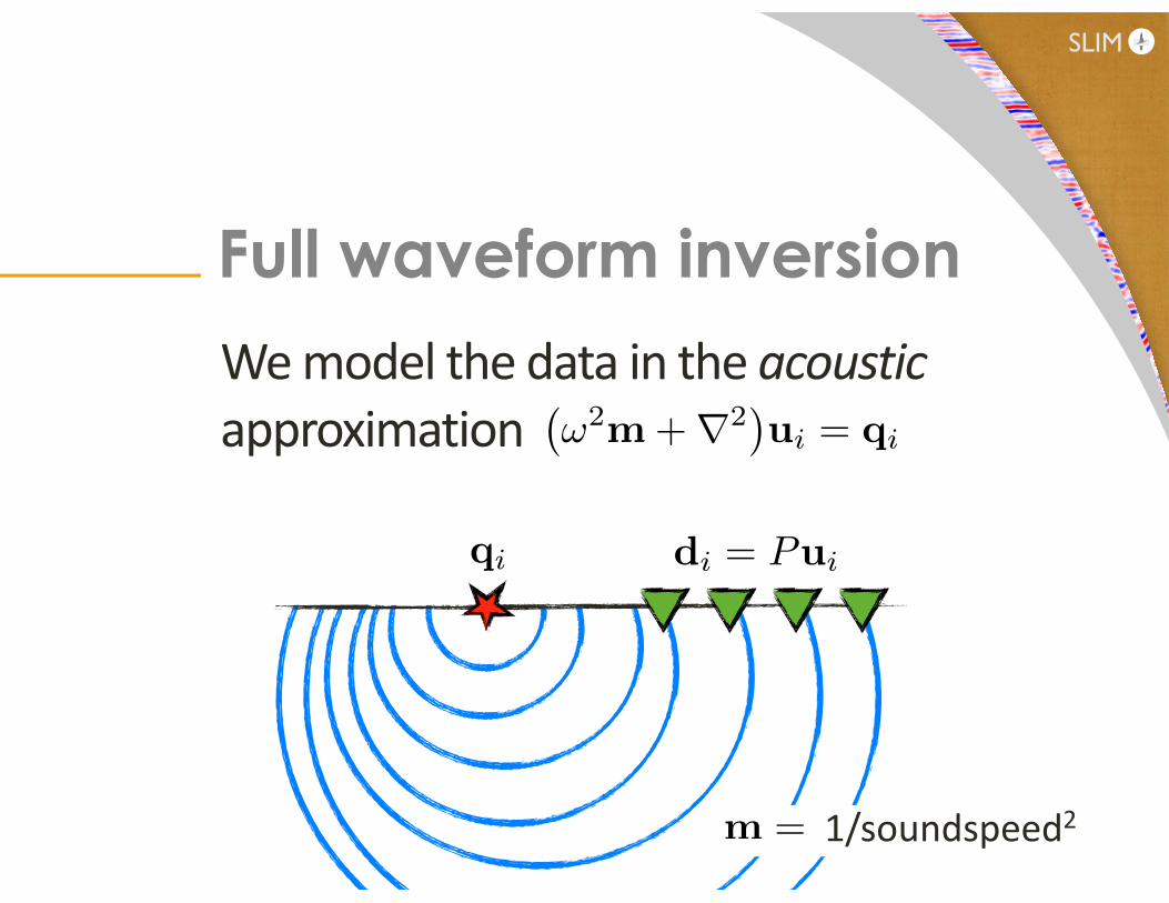
We  model  the  data  in  the  acoustic  approximation

Full waveform inversion

1/soundspeed2m =

�!2m+r2

�ui = qi

di = Puiqi

SLIM

Realistic  scale  (3D):  •                          unknowns•                              measurements• 3D  Helmholtz  equation  is  non-­‐trivial  to  solve.

Full waveform inversion

O(1015)

O(109)

SLIM

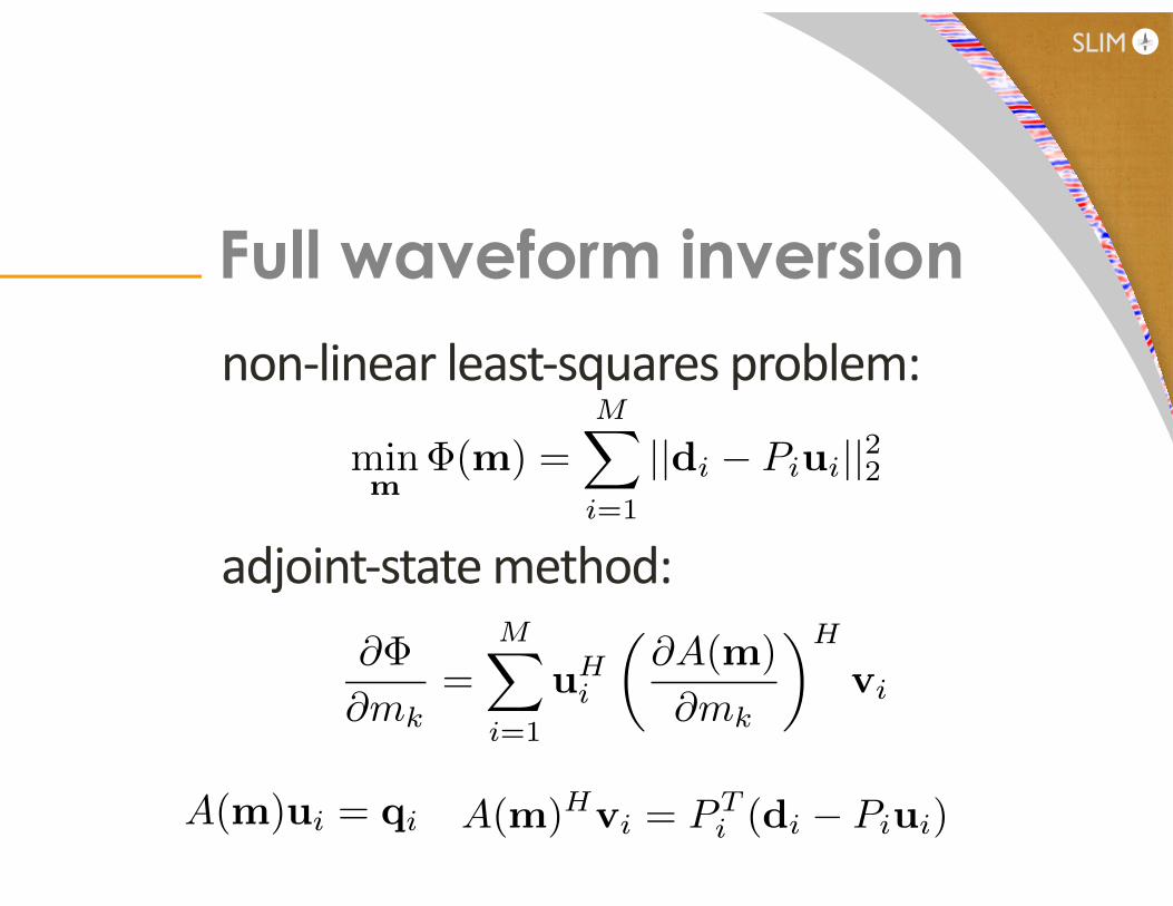
non-­‐linear  least-­‐squares  problem:

adjoint-­‐state  method:

Full waveform inversion

@�

@mk=

MX

i=1

uHi

✓@A(m)

@mk

◆H

vi

A(m)ui = qi A(m)Hvi = PTi (di � Piui)

minm

�(m) =MX

i=1

||di � Piui||22

SLIM

Camembert  example

Full waveform inversion

x [km]

z [k

m]

0 0.5 1

0

0.2

0.4

0.6

0.8

12.3

2.4

2.5

2.6

2.7

[Gauthier  et  al  ’86]

SLIM

models  explain  ~95%  of  the  data

Full waveform inversion

x [km]

z [k

m]

0 0.5 1

0

0.2

0.4

0.6

0.8

12.3

2.4

2.5

2.6

2.7

x [km]

z [k

m]

0 0.5 1

0

0.2

0.4

0.6

0.8

12.3

2.4

2.5

2.6

2.7

reflection transmission

SLIM

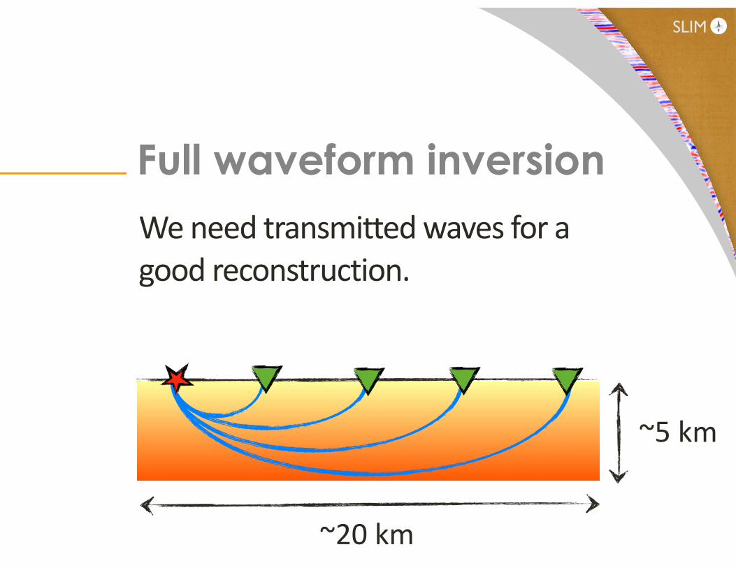
Full waveform inversion

We  need  transmitted  waves  for  a  good  reconstruction.

~20  km

~5  km

SLIM

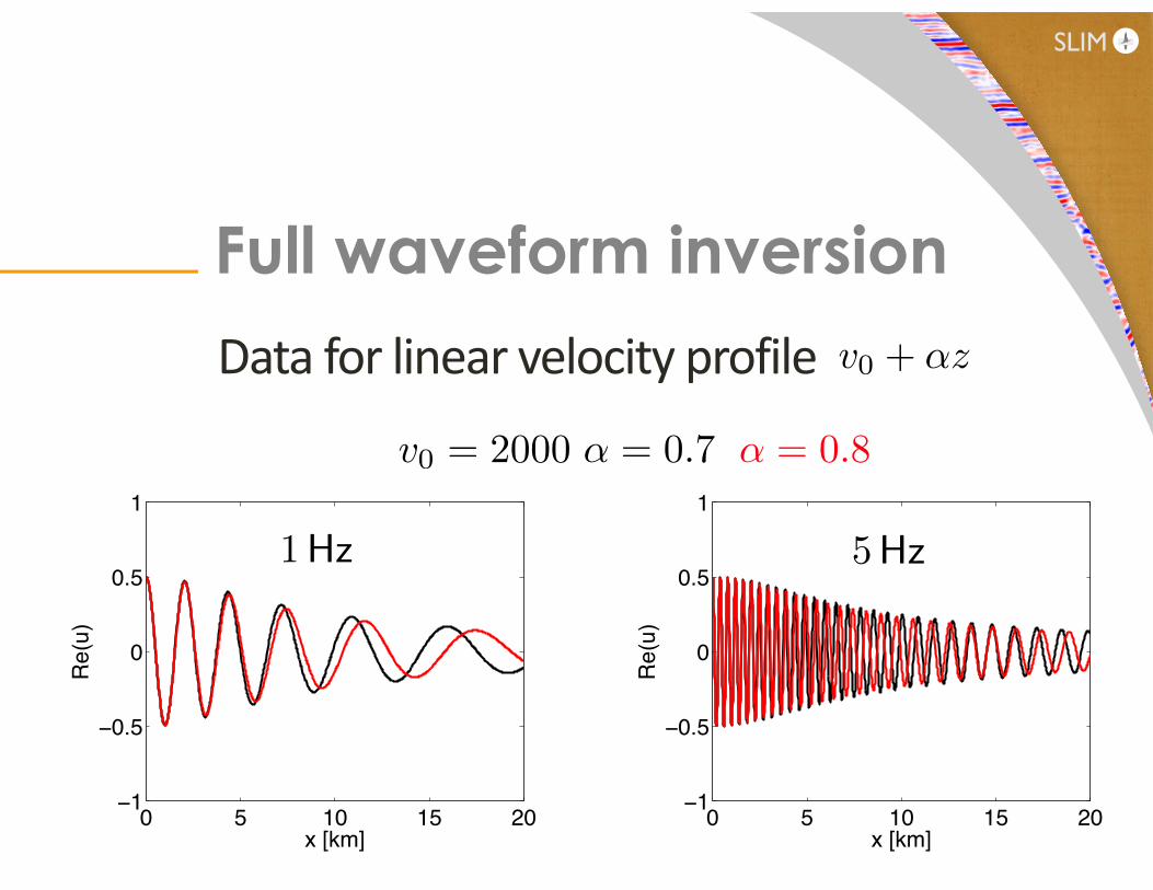
Data  for  linear  velocity  profile

Full waveform inversion

0 5 10 15 20−1

−0.5

0

0.5

1

x [km]

Re(

u)

0 5 10 15 20−1

−0.5

0

0.5

1

x [km]

Re(

u)

v0 + ↵z

↵ = 0.7 ↵ = 0.8v0 = 2000

1Hz 5Hz

SLIM

LS  misfit  as  a  function  of  

Full waveform inversion

v0 [m/s]

_ [1

/s]

0.6 0.8 1

1500

2000

2500v0 [m/s]

_ [1

/s]

0.6 0.8 1

1500

2000

2500

(v0,↵)

1Hz 5Hz

[Mulder  et  al  ’08]

local  minima

SLIM

These  observations  motivate  continuation  strategies• low  -­‐  high  frequency• small  -­‐  large  offsets• early  -­‐  late  arrival  times

Full waveform inversion

[Bunks  ’95;  Pra`  ’98;Shin  ’08,’09]

SLIM

                                                           is  twice  differentiable                            is  the  primary  parameter,                        is  a  set  of  auxiliary  parameters,typically  

General formulation

m 2 Rn

✓ 2 Rk

�i : Rn ⇥ Rk ! R

k ⌧ n

minm,✓

�(m, ✓) =MX

i=1

�i(m, ✓)

SLIM

example  1:least-­‐squares  with  source  calibration

         is  a  source-­‐weight

General formulation

✓i

�i(m, ✓) = ||di � ✓iFi(m)||22

SLIM

example  2:Gaussian  ML  estimation

General formulation

P✓(m,d) =Y

i

(2⇡✓i)�N/2

exp

�� 1

2 ||di � Fi(m)||22/✓i�

�i(m, ✓) = N log(2⇡✓i) + ✓�1i ||di � Fi(m)||22

di = Fi(m) + ✏i, ✏i ⇠ N (0, ✓iI)

SLIM

example  3:Robust  ML  estimation

for  Students  T:

General formulation

di = Fi(m) + ✏i, ✏i ⇠ heavy-tailed distribution

�i(m, ✓) = ⇢✓(di � Fi(m))

⇢✓(r) = �N log

�(

✓+12 )

�(

✓2 )p⇡✓

!+

✓ + 1

2

NX

j=1

log(1 + r2j/✓)

SLIM

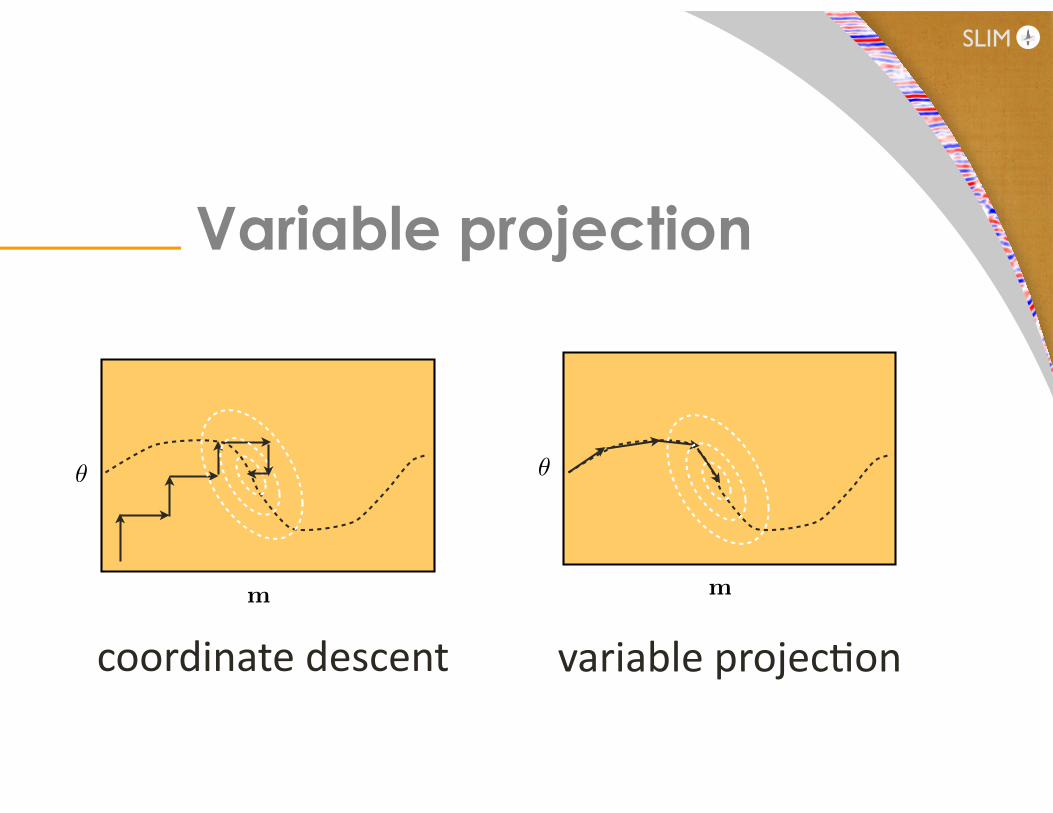
Consider  cases  where  solving

for  fixed              is  `easy’,  and  define

with

Variable projection

min✓

�(m, ✓)

m

✓̄(m) = argmin✓

�(m, ✓)

�̄(m) = min✓

�(m, ✓) = �(m, ✓̄(m))

SLIM

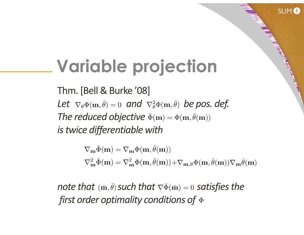
Thm.  [Bell  &  Burke  ’08]Let                                                      and                                        be  pos.  def.The  reduced  objective  is  twice  differentiable  with

note  that                      such  that                                        satisfies  the  first  order  optimality  conditions  of  

Variable projection

r2✓�(m, ✓̄)r✓�(m, ✓̄) = 0

�̄(m) = �(m, ✓̄(m))

rm�̄(m) = rm�(m, ✓̄(m))

r2m�̄(m) = r2

m�(m, ✓̄(m))+rm,✓�(m, ✓̄(m))rm✓̄(m)

r�̄(m̄) = 0(m̄, ✓̄)

�

SLIM

Variable projection

m

✓

m

✓

coordinate  descent variable  projeccon

SLIM

• Faster  convergence  for                                                                    [Golub&Peyrera  ’73,  Kaufman  ’74,  Osborne  ’07]

• Extended  least-­‐squares  [Bell  &  Burke  ’96]

• Extension  to  general  class,  easy  design  of  GN  or  QN  methods  [Aravkin  &  TVL  ’12]

Variable projection||A(m)✓ � d||22

SLIM

• Source  calibration• LS  variance  estimation• Robust  T  data-­‐fitting

Applications

SLIM

Source estimation

x [km]

z [k

m]

0 5 10 15

0

1

22

3

4

5 10 15 200

20

40

60

80

100

frequency [1/s]

ampl

itude

x [km]

z [k

m]

0 5 10 15

0

1

22

3

4

source-­‐weight

true  model

recovered  model

[TVL  ’12]

SLIM

add  noise  with  different  variance  

LS variance estimation

x [km]

z [k

m]

0 0.5 1 1.5 2 2.5 3

0

0.5

1

1.5

2

x [km]

z [k

m]

0 0.5 1 1.5 2 2.5 3

0

0.5

1

1.5

2

0 10 20 30 40 500.8

0.85

0.9

0.95

1

iteration

rel. m

od

el e

rro

r

fixed  variance

est.  variance

||mk�

m⇤ || 2/||m

0�

m⇤ || 2

[Aravkin  &  TVL  ’12]

SLIM

densities  &  penalties

Robust data-fitting

Gaussian,  Laplace  and  Students  T

SLIM

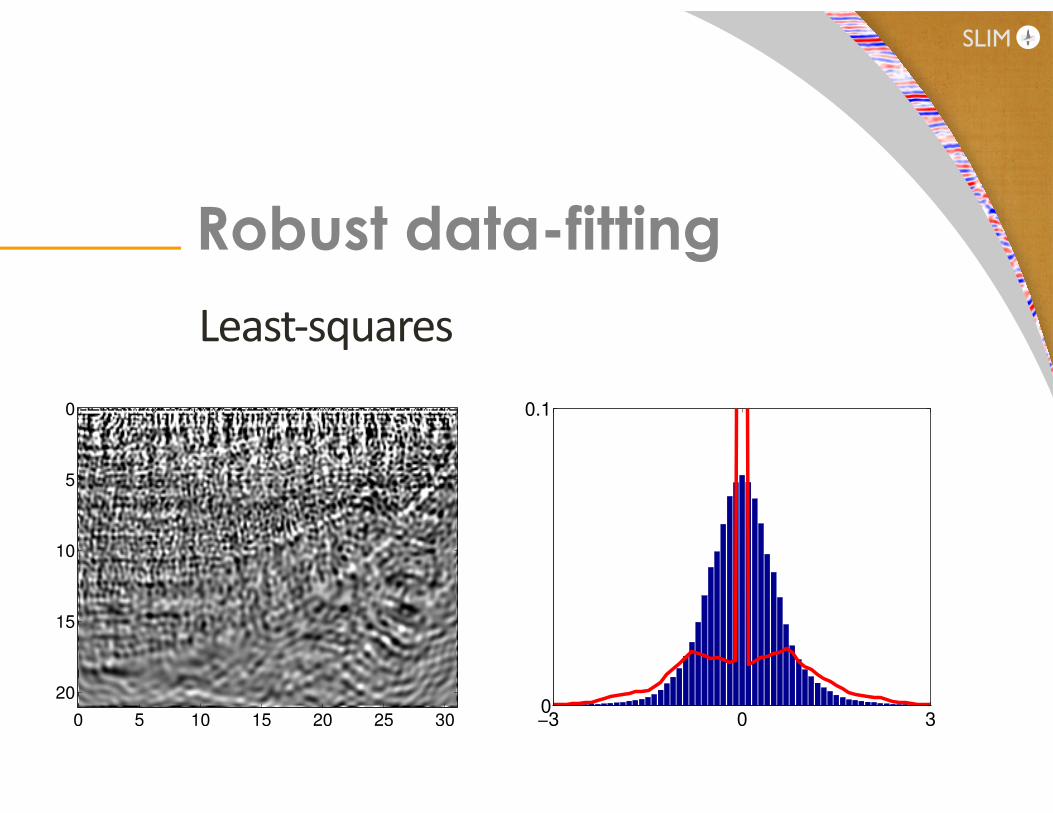
Recover  from  data  with  50%  outliers

Robust data-fitting

0 5 10 15 20 25 30

0

5

10

15

20

!3 0 30

0.1

di � F [mtrue]qi mtrue

[Friedlander  ’12]

SLIM

Least-­‐squares

Robust data-fitting

0 5 10 15 20 25 30

0

5

10

15

20

!3 0 30

0.1

SLIM

`Laplace’

Robust data-fitting

0 5 10 15 20 25 30

0

5

10

15

20

!3 0 30

0.1

SLIM

Students  T  

Robust data-fitting

0 5 10 15 20 25 30

0

5

10

15

20

!3 0 30

0.1

SLIM

Robust data-fitting

x [km]

z [k

m]

0 0.2 0.4 0.6 0.8 1

0

0.2

0.4

0.6

0.8

1 !100

!50

0

50

100

150

200

x [km]

z [k

m]

0 0.2 0.4 0.6 0.8 1

0

0.2

0.4

0.6

0.8

1 !100

!50

0

50

100

150

200

x [km]

z [k

m]

0 0.2 0.4 0.6 0.8 1

0

0.2

0.4

0.6

0.8

1 !100

!50

0

50

100

150

200

true  model fixed  df.

Students  t  with  varying  degrees-­‐of-­‐freedom

fi`ed  df.

SLIM

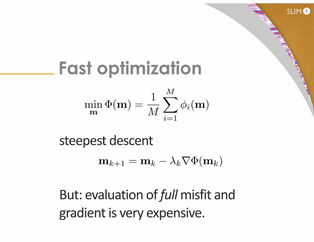
steepest  descent

But:  evaluation  of  full  misfit  and  gradient  is  very  expensive.

Fast optimization

minm

�(m) =1

M

MX

i=1

�i(m)

mk+1 = mk � �kr�(mk)

SLIM

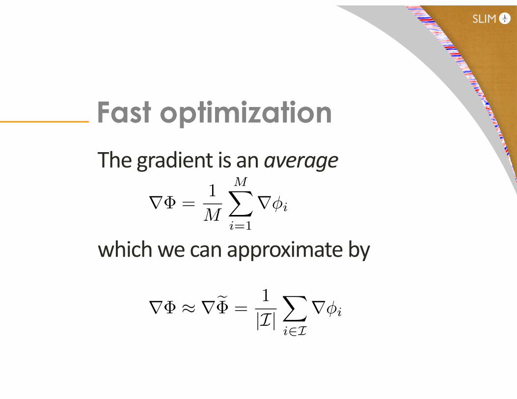
The  gradient  is  an  average

which  we  can  approximate  by

Fast optimization

r� ⇡ re� =1

|I|X

i2Ir�i

r� =1

M

MX

i=1

r�i

SLIM

Gradient  descent  with  errors:

stochastic/incremental  gradient  require                                    and  have  sublinear  convergence  rate

Optimization

re�k = r�k + ek

E(ek) = 0

SLIM

Instead,  require  that              and  Then

where  Linear  convergence  if

Optimization

0 < c < 1

[Friedlander  &  Schmidt  ’12]

||ek|| Bk

limk!1

Bk+1/Bk 1

Bk = O(�k)

�(mk)� �(m⇤) = ck(�(mk)� �(m0)) +O(max{Bk, c

k})

SLIM

Decrease  the  error  by  adding  elements  to  the  batch• in  a  pre-­‐scribed  order• random  without  replacement• random  with  replacement

Optimization

ek =M � |Ik|M |Ik|

X

i2Ik

r�i +1

M

X

i 62|I|

r�i

SLIM

Error  in  the  gradient

Optimization

0 50 100 150

106

107

K

error

0 20 40 60 80 10010−4

10−3

10−2

10−1

100

batch size

erro

r

worst  casew  replacementw/o  replacement

natural  orderw  replacementw/o  replacement

error  bound numerical  result

SLIM

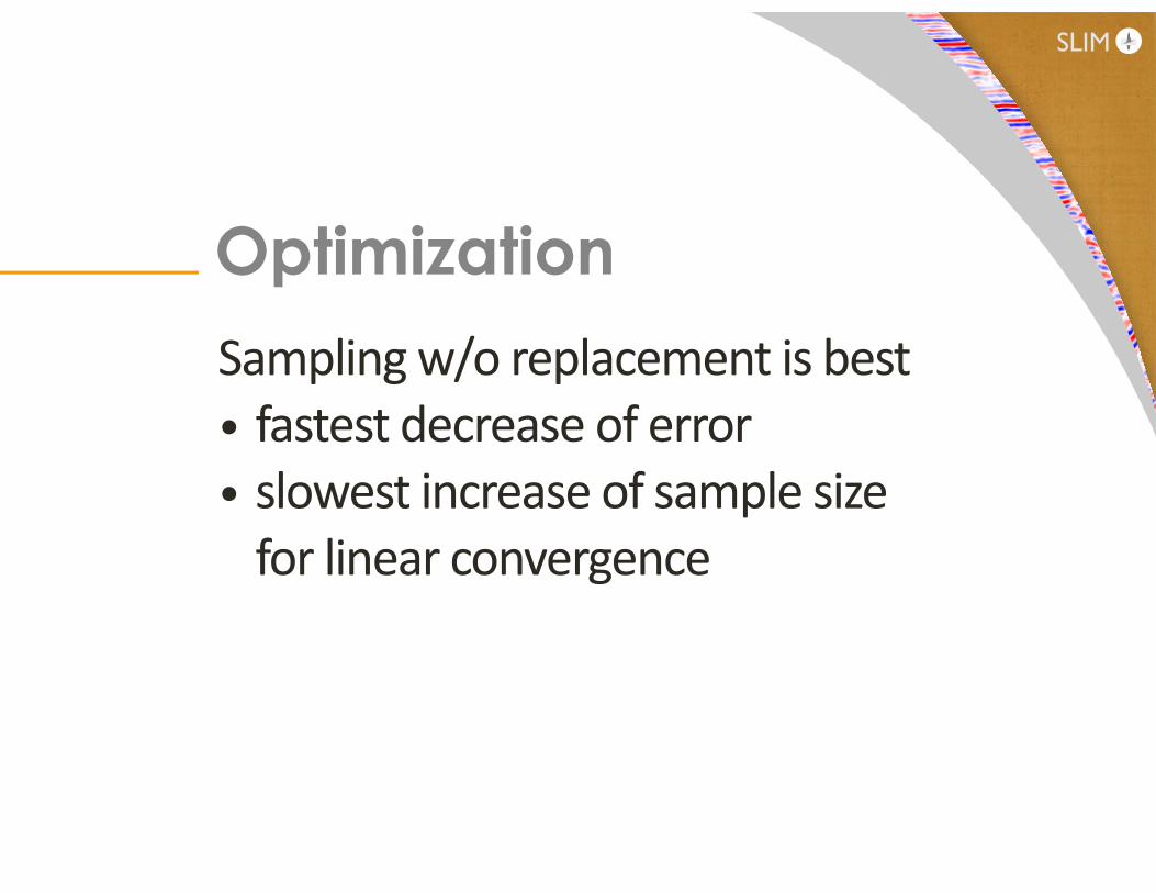
Sampling  w/o  replacement  is  best• fastest  decrease  of  error• slowest  increase  of  sample  size  for  linear  convergence

Optimization

SLIM

Optimization

x [km]

z [k

m]

0 2 4 6

0

1

2

x [km]z

[km

]0 2 4 6

0

1

2

100 200 300 400 500

0.7

0.75

0.8

0.85

0.9

# passes through data

rel.

mod

el e

rror

batchingfull

[van  Leeuwen  et  al  ’11]

10  x  speedup

||mk�

m⇤ || 2/||m

0�

m⇤ || 2

SLIM

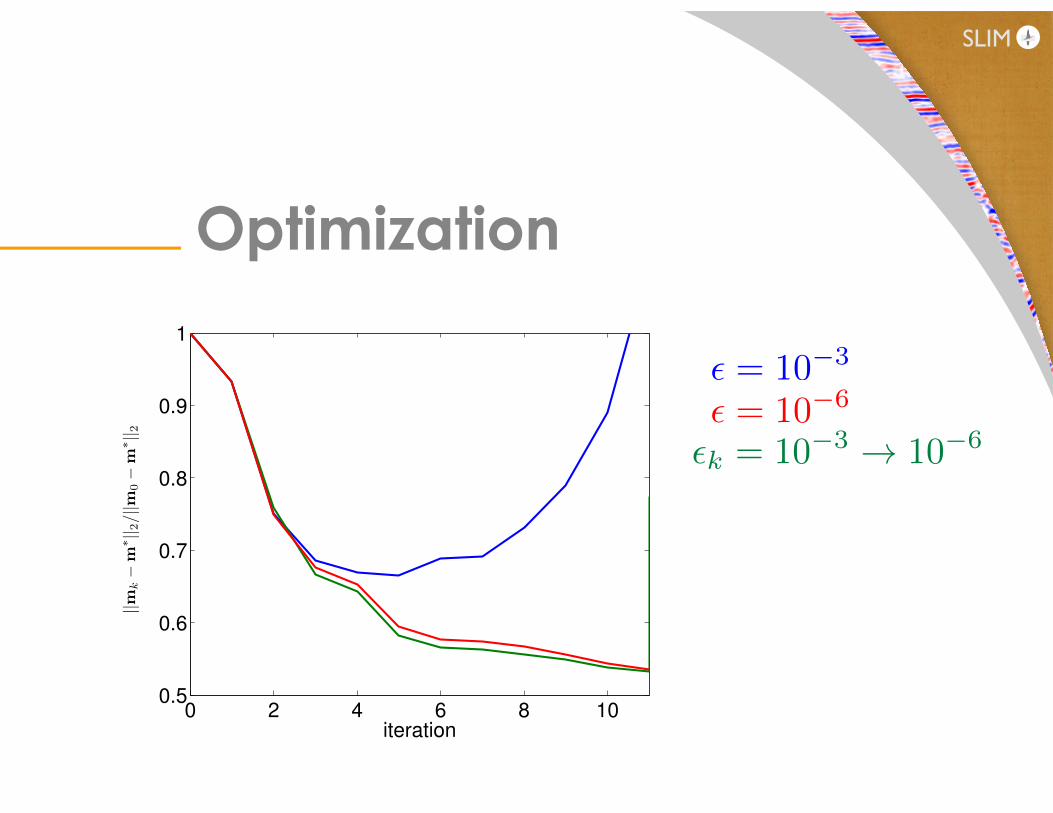
Decrease  error  by  controlling  accuracy  of  PDE-­‐solves

Optimization

A(m)ui = qi

A(m)Hvi = PTi (di � Piui)

SLIM

Optimization

x [km]

z [k

m]

y = 0.5 km

0 0.5 1

0

0.5

1x [km]

y [k

m]

z = 0.5 km

0 0.5 1

0

0.5

1y [km]

z [k

m]

x = 0.5 km

0 0.5 1

0

0.5

1

x [km]

z [k

m]

y = 0.5 km

0 0.5 1

0

0.5

1x [km]

y [k

m]

z = 0.5 km

0 0.5 1

0

0.5

1y [km]

z [k

m]

x = 0.5 km

0 0.5 1

0

0.5

1x [km]

z [k

m]

y = 0.5 km

0 0.5 1

0

0.5

1x [km]

y [k

m]

z = 0.5 km

0 0.5 1

0

0.5

1y [km]

z [k

m]

x = 0.5 km

0 0.5 1

0

0.5

1

✏ = 10�3

✏ = 10�6 ✏k = 10�3 ! 10�6

SLIM

Optimization

0 2 4 6 8 100.5

0.6

0.7

0.8

0.9

1

iteration

rel. m

od

el e

rro

r

✏ = 10�3

✏ = 10�6

✏k = 10�3 ! 10�6

||mk�

m⇤ || 2/||m

0�

m⇤ || 2

SLIM

• Novel  method  for  estimation  of  auxiliary  parameters

• Improved  recovery  on  very  noisy  data  by  using  Students  T

• Order  of  magnitude  speedup  by  working  on  subsets  of  the  data

Summary

This  work  was  in  part  financially  supported  by  the  Natural  Sciences  and  Engineering  Research  Council  of  Canada  Discovery  Grant  (22R81254)  and  the  Collaborative  Research  and  Development  Grant  DNOISE  II  (375142-­‐08).  This  research  was  carried  out  as  part  of  the  SINBAD  II  project  with  support  from  the  following  organizations:  BG  Group,  BGP,  BP,  Chevron,  ConocoPhillips,  Petrobras,  PGS,  Total  SA,  and  WesternGeco.

Acknowledgements

Thank  you!

Further readingA.Y.  Aravkin  and  T.  van  Leeuwen  -­‐  Escmacng  nuisance  parameters  in  inverse  problems.  Inverse  Problems  (accepted),  2012.

A.  Aravkin,  M.P.  Friedlander,  F.J.  Herrmann  and  T.  van  Leeuwen  -­‐  Robust  inversion,  dimensionality  reduccon  and  randomized  sampling.  Mathemaccal  Programming,  2012.

T.  van  Leeuwen  and  F.J.  Herrmann  -­‐  Fast  waveform  inversion  without  source  encoding.  Geophysical  Prospeccng,  2012

B.M.  Bell  and  J.V.  Burke.  Algorithmic  differen9a9on  of  implicit  func9ons  and  op9mal  values.Advances  in  Automa9c  Differen9a9on,  2008.B.M.  Bell,  J.V.  Burke,  and  A.  Schumitzky.  A  rela9ve  weigh9ng  method  for  es9ma9ng  parameters  and  variances  in  mul9ple  data  sets.  Comp.  Stat.  &  Data  Analysis,  1996.Gene  Golub  and  Victor  Pereyra.  Separable  nonlinear  least  squares:  the  variable  projec9on  method  and  its  applica9ons.  Inverse  Problems,  19(2):R1,  2003.G.H.  Golub  and  V.  Pereyra.  The  differen9a9on  of  pseudo-­‐inverses  and  nonlinear  least  squares  which  variables  separate.  SIAM  J.  Numer.  Anal.,  10(2):413–432,  1973.M.  R.  Osborne.  Separable  least  squares,  variable  projec9on,  and  the  Gauss-­‐Newton  algorithm.  Electronic  Transac9ons  on  Numerical  Analysis,  28(2):1–15,  2007.R  G  Praa,  C  Shin,  and  Gj  Hicks.  Gauss-­‐newton  and  full  newton  methods  in  frequency-­‐space  seismic  waveform  inversion.  Geophysical  Journal  Interna9onal,  1998.M.  P.  Friedlander  and  M.  Schmidt.  Hybrid  determinis9c-­‐stochas9c  methods  for  data  fidng.  SIAM  J.  Scien9fic  Compu9ng,  34(3),  2012  (submiaed  April  2011)