A Plane Symmetric 6R Foldable Ring

A.D. Viquerata,, T. Huttb, S.D. Guesta,

aDepartment of Engineering, University of Cambridge, Trumpington Street, Cambridge CB2 1PZ, UKbDepartment of Mechanical Engineering, Imperial College London, Exhibition Road, South Kensington, London SW7 2AZ, UK

Abstract

The design of a deployable structure which deploys from a compact bundle of six parallel bars to a rectangular ring isconsidered. The structure is a plane symmetric Bricard linkage. The internal mechanism is described in terms of itsDenavit-Hartenberg parameters; the nature of its single degree of freedom is examined in detail by determining theexact structure of the system of equations governing its movement; a range of design parameters for building feasiblemechanisms is determined numerically; and polynomial continuation is used to design rings with certain specifieddesirable properties.

Keywords: Numerical continuation, Deployable structure, Bricard linkage

1. Introduction

Several different types of foldable frames, which in their deployed configurations form (often regular) polygons,have appeared in literature in the past 40 years. Bennett or Bricard [1] linkages are frequently used as the basislinkages for foldable deployable frames. An early example appears in [2], in which an even number of bars are linkedtogether in such a way that they can be folded into a tight bundle, and unfolded to form a regular polygon. In the sixbar case, a three-fold symmetric linkage results [3], while in the four bar case, a Bennett linkage is formed [4, 5]. Fourbar foldable frames have been extensively examined [6, 4, 7]. For the six-bar case, Wohlhart [8, 9] and Racilla [10]have focussed on the kinematics of the trihedral, or ‘rectangular’ member of the Bricard family. In [11], Pellegrinoet al. proposed a new family of six bar foldable frames. A two-fold symmetric member of this family has beenproposed as a support for a solar blanket, and its kinematics examined numerically [12, 13]. Recently, the two-foldsymmetric 6R foldable frame was identified as a special line and plane symmetric Bricard linkage [14]. This particularvariant does, however, suffer from problems with bifurcations (although certain designs avoid this). If one of the twoplanes of symmetry is removed, a mobile 6R ring which experiences fewer problems with bifurcations remains. Anexample is shown in Figure 1. In this paper, a greater understanding of the plane symmetric 6R foldable ring issought by first identifying the ring as a plane symmetric Bricard linkage, examining the nature of its mobility using acascade of homotopies [15] to identify positive dimensional solution sets (an application of polynomial continuation),determining a range of design parameters for building feasible mechanisms of this type, deriving a closed formexpression for the linkage’s kinematics, and finally employing polynomial continuation, again, in an attempt to designa family of plane symmetric 6R foldable rings with certain desirable practical properties.

2. Linkage Specification

The two-fold symmetric ring of [14] has two different bar lengths (l1 and l2), and the bars are all tilted fromthe vertical by a single angle µ. Square cross-sectioned, prismatic (i.e., untwisted) bars were used. By contrast, the6R linkage considered here has all six bar lengths the same (l), and four separate bar tilt angles (α′1, α

′2, β1 and β2),

introducing a requirement that, if the bars have a square cross-section, some of the bars must be twisted in order to

Email address: sdg@eng.cam.ac.uk (S.D. Guest)

Preprint submitted to Mechanism and Machine Theory August 16, 2012

match the prescribed tilt angles at each end. A simplified diagram of the deployed linkage with all design parameterslabelled is given in Figure 3, while a representation of the physical linkage is given in Figure 4, in which the twistsin the bars are clearly visible. While a square cross-section is not required to construct the linkage, it does aid invisualising the bar twist.

Figure 1: Folding process for a linkage with parameters α1 = π/4, α2 = −π/4 and γ = π/2. Each bar is shown as atwisted prismatic bar with square cross-section.

Figure 2: The folding of a wooden model of the linkage shown in Figure 1.

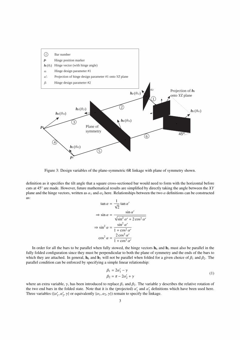
There are six hinges (labelled h1 − h6), each with a single rotational degree of freedom connecting the bars in aclosed loop. The plane of symmetry is preserved through the folding motion. It is labelled as the XZ plane in the fullydeployed/open configuration, shown in Figure 3. The plane contains the points p6 and p3, and the vectors h6 and h3,which are inclined to the Z axis by angles β1 and β2 respectively. Also when deployed, hinges h1 and h2 lie in planesrotated from the YZ plane by 45◦ about the Z axis. The angles these hinges form to the horizontal can be specifiedin two important ways. When constructing physical models of the plane-symmetric 6-bar, the most intuitive form isobtained by taking the projection of the hinges onto the YZ plane, and considering the angle formed between thatprojection and the XY plane, labelled here as α′1 and α′2. This projection is shown in Figure 3. This is a more intuitive

2

Y

XZ

h1 (θ61)

45º

Plane of symmetry

Projection of h1 onto YZ planeh2 (θ12)

h3 (θ23)h4 (θ34)

h5 (θ45)

h6 (θ56)

1

2

3

4

5

6β1

β2

α1

α2

α'1

p1

p2

p3

p4

p5

p6

i Bar numberpi Hinge position markerhi (θji) Hinge vector (with hinge angle)

αi Hinge design parameter #1

α'i Projection of hinge design parameter #1 onto YZ plane

βi Hinge design parameter #2

Figure 3: Design variables of the plane-symmetric 6R linkage with plane of symmetry shown.

definition as it specifies the tilt angle that a square cross-sectioned bar would need to form with the horizontal beforecuts at 45◦ are made. However, future mathematical results are simplified by directly taking the angle between the XYplane and the hinge vectors, written as α1 and α2 here. Relationships between the two α definitions can be constructedas:

tanα =1√

2tanα′

⇒ sinα =sinα′√

sin2 α′ + 2 cos2 α′

⇒ sin2 α =sin2 α′

1 + cos2 α′

cos2 α =2 cos2 α′

1 + cos2 α′

In order for all the bars to be parallel when fully stowed, the hinge vectors h6 and h3 must also be parallel in thefully folded configuration since they must be perpendicular to both the plane of symmetry and the ends of the bars towhich they are attached. In general, h6 and h3 will not be parallel when folded for a given choice of β1 and β2. Theparallel condition can be enforced by specifying a simple linear relationship:

β1 = 2α′1 − γβ2 = π − 2α′2 + γ

(1)

where an extra variable, γ, has been introduced to replace β1 and β2. The variable γ describes the relative rotation ofthe two end bars in the folded state. Note that it is the (projected) α′1 and α′2 definitions which have been used here.Three variables ({α′1, α

′2, γ} or equivalently {α1, α2, γ}) remain to specify the linkage.

3

h1

h2

h3

h4

h5

h6

Figure 4: Example of plane-symmetric 6R foldable linkage with visible bar twist for α1 = π/4, α2 = −π/4 andγ = π/2.

It can be shown that hinges 1 and 2 have maximum opening angles (assuming θi j = 0 when fully deployed):

θ61max = π − 2 tan−1

tan α′1√2 + tan2 α′1

= π − cos−1(cos2 α′1)

θ12max = π − 2 tan−1

tan α′2√2 + tan2 α′2

= π − cos−1(cos2 α′2)

(2)

At these maximum angles, bars 6 and 2 are both colinear with bar 1, indicating full folding of the linkage. Thesedefinitions will be useful for simulation purposes later.

3. Identification as a Bricard Plane Symmetric Case

Figure 5 illustrates the Denavit-Hartenberg parameters for the plane symmetric Bricard linkage. The relationships(implied by symmetry) between these parameters (from [16]) are:

a61 = a56 , a12 = a45 , a23 = a34

α61 + α56 = α12 + α45 = α23 + α34 = π

R6 = R3 = 0 , R1 = R5 , R2 = R4

(3)

It is possible to derive a relationship between the design variables α1, α2, β1 and β2 of the plane symmetric 6Rfoldable ring, and the Denavit-Hartenberg parameters. This is achieved by solving a series of simple linear equationswhich arise from the linkage’s geometry. Start with the link between hinges 6 and 1. The Bricard linkage joints must

4

h3

α23a23

R2

a12

α12

h2

α61

R1

h1

a61

h6

h5

h4

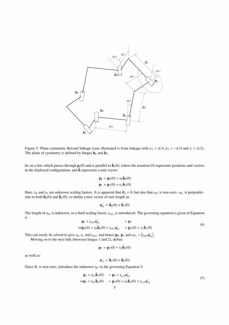
Figure 5: Plane symmetric Bricard linkage (case illustrated is from linkage with α1 = π/4, α2 = −π/4 and γ = π/2).The plane of symmetry is defined by hinges h6 and h3.

lie on a line which passes through pi(0) and is parallel to hi(0), where the notation (0) represents positions and vectorsin the deployed configuration, and h represents a unit vector:

p6 = p6(0) + tl6h6(0)

p1 = p1(0) + tl1h1(0)

Here, tl6 and tl1 are unknown scaling factors. It is apparent that R6 = 0, but also that a61 is non-zero. a61 is perpendic-ular to both h6(0) and h1(0), so define a new vector of unit length as:

a′61 = h6(0) × h1(0)

The length of a61 is unknown, so a third scaling factor, ta61, is introduced. The governing equation is given in Equation4.

p6 + ta61a′61 = p1

⇒p6(0) + tl6h6(0) + ta61a′61 = p1(0) + tl1h1(0)(4)

This can easily be solved to give tl6, tl1 and ta61, and hence p6, p1 and a61 =∣∣∣ta61a′61

∣∣∣.Moving on to the next link (between hinges 1 and 2), define:

p2 = p2(0) + tl2h2(0)

as well as:a′12 = h1(0) × h2(0)

Since R1 is non-zero, introduce the unknown tR1 to the governing Equation 5.

p1 + tR1h1(0) = p2 + ta12a′12

⇒p1 + tR1h1(0) = p2(0) + tl2h2(0) + ta12a′12

(5)

5

From this tl2, tR1 and ta12 can be found, which in turn gives p2, R1 = tR1 and a12 =∣∣∣ta12a′12

∣∣∣.Finally, consider the link between hinges 2 and 3 by defining:

p3 = p3(0) + tl3h3(0)

as well as:a′23 = h2(0) × h3(0)

and Equation 6.p2 + tR2h2(0) = p3 + ta23a′23

⇒p2 + tR2h2(0) = p3(0) + tl3h3(0) + ta23a′23

(6)

From this tl3, tR2 and ta23 can be found, which in turn gives p3, R2 = tR2 and a23 =∣∣∣ta23a′23

∣∣∣.The important parameters (obtained using Mathematica [17]) are:

a61

l=

√1 −

4 cos2 (α1)

2√

2 sin (2α1) sin (2β1) + (3 cos (2α1) − 1) cos (2β1) + cos (2α1) + 5

a12

l= 2

√sin2 (α1 − α2)

2 cos (2α1) + 4 sin2 (α1) cos (2α2) + 6

a23

l=

√1 −

4 cos2 (α2)

−2√

2 sin (2α2) sin (2β2) + (3 cos (2α2) − 1) cos (2β2) + cos (2α2) + 5

and

R1

l=√

2 4 cos (α1)

2√

2 sin (2α1) sin (2β1) + (3 cos (2α1) − 1) cos (2β1) + cos (2α1) + 5−

2 (cos (α1) + sin (α1) sin (α2) cos (α2))

cos (2α1) + 2 sin2 (α1) cos (2α2) + 3

)

R2

l=√

2 sec (α2) .− 4 cos2 (α2)

−2√

2 sin (2α2) sin (2β2) + (3 cos (2α2) − 1) cos (2β2) + cos (2α2) + 5+

sin (2α1) sin (2α2) + 4 cos (2α2) + 4 sin2 (α2) cos (2α1) + 82 cos (2α1) + 4 sin2 (α1) cos (2α2) + 6

− 1)

The twist angles can be simply determined as:

α61 = cos−1(〈h6(0), h1(0)〉

)α12 = cos−1

(〈h1(0), h2(0)〉

)α23 = cos−1

(〈h2(0), h3(0)〉

)As a numerical example, consider the case of α1 = π/4, α2 = −π/4, and β1 = β2 = 0 (γ = π/2). This can be

written in terms of Denavit-Hartenberg parameters for the plane symmetric case:

a61

l=

1√

2,

a12

l=

√23,

a23

l=

1√

2R1

l=

23,

R2

l= −

23

α61 =π

4, α12 =

2π3, α23 =

3π4

6

4. Loop Closure Equations

It is possible to construct a set of loop closure equations by defining coordinate systems attached to each link, andthen deriving the transfer matrices which describe the transformation from one coordinate system to the next. Thismethod is illustrated in [14] and [13], where it is used to simulate the motion of closed loop linkages, and to studytheir bifurcations. A transfer matrix is typically 4 × 4, and consists of a 3 × 3 rotation matrix, say R, and a 3 × 1translation vector, say v. These parts are arranged as:

T =

[R v

0 0 0 1

]If a coordinate system is attached to the end of a link in a linkage, then a transfer matrix can be used to rotate andtranslate it to the location of the coordinate system attached to an adjacent link in a single operation. Repeating thisoperation around a linkage which is also a closed loop will eventually lead back to the original link. Mathematically,this can be expressed as:

F = T61T56T45T34T23T12 − I = 0

where Tab defines the transfer between the coordinate system attached to link a to that attached to b. The coordinatesystem at each joint is aligned so that the z-axis is aligned with the hinge axis. Before each translation, the x-axisis rotated such that it points along the current bar towards the next joint. As there are single degree of freedomconnections between the links, each transfer matrix can be separated into a part which deals only with rotation aboutthe z-axis, L3, and a part which relates to the unchanging geometry of the link, T L

ab, and Tab = T LabL3(θab). The

equations above then become:

F = T L61L3(θ61)T L

56L3(θ56)T L45L3(θ45)T L

34L3(θ34)T L23L3(θ23)T L

12L3(θ12) − I = 0 (7)

Explicitly, the transfer matrices for each of the six links are:

T L12 = L1(β2)ML3(π/4)L1(α2 − π/2)

T L23 = L1(π/2 − α2)L3(π/4)ML1(−β2)

T L34 = L1(π/2 − α1)L3(π/4)ML3(π/4)L1(α2 − π/2)

T L45 = L1(−β1)ML3(π/4)L1(α1 − π/2)

T L56 = L1(π/2 − α1)L3(π/4)M(π/4)L1(β1)

T L61 = L1(π/2 − α2)L3(π/4)ML3(π/4)L1(α1 − π/2)

(8)

where L1 is a rotation about the x-axis, and M defines a translation of length l along each link:

M =

1 0 0 −l0 1 0 00 0 1 00 0 0 1

The single off-diagonal entry in matrix M has a negative sign because the effect of applying M to a point in spaceis to rewrite that point as a location in the basis of the new, translated coordinate system. Shifting a coordinatesystem in the positive x-direction requires the inclusion of a negative term in the (1, 4) location of matrix M. Thematrix Equation 7 can be separated into six individual equations which together ensure loop closure. As in [13], thestrictly upper triangular part of this matrix equation provides six independent scalar equations necessary to form asquare system:

F(θ12, θ23, θ34, θ45, θ56, θ61) =

F1,2F1,3F1,4F2,3F2,4F3,4

= 0 (9)

7

Having derived these loop closure equations, it is possible to simulate the motion of the linkage using a type ofpredictor-corrector approach detailed in [13] and [14]. One particularly useful by-product of this method is a matrixwhose singular values can be used to examine the linkage’s mobility at each point of the unfolding process. Thestructure of these equations will be examined in the following section.

5. Examination of Mobility using a Cascade of Homotopies

The plane-symmetric six-bar ring can be described as an over-constrained mechanism, or as possessing a geomet-ric degree of freedom. This implies that it does not satisfy the Kutzbach Criterion [18], which must be due to somespecial feature of the linkage’s geometry, in this case its symmetry. It is possible to determine mathematically if alinkage is likely to possess a geometric degree of freedom, and if so, of what order, and in how many disconnectedsets, by using the method of witness sets described in [19] and [15]. This type of analysis forms part of a broaderfield known as Polynomial Continuation [20, 21, 22] in which all finite solutions to a system of polynomial equationsare found by first finding the solutions to a separate system of equations with a similar polynomial structure, and thennumerically tracking these known solutions into those of the unknown system. The method can be used to identifyfinite, geometrically isolated solutions, or with a few additions, to find curves of solutions through the solution space.

The loop closure equation of section 4 can be simplified by assuming that hinge angles reflected in the plane ofsymmetry will be equal, as:

θ12 = θ34

θ45 = θ61

Recall that these hinge angles are defined as being zero when the foldable ring is in the fully deployed state. Finally,the maximum order of the resulting polynomial closure equations can be reduced by rearrangement into the form ofEquation 10.

F′ =L3(θ61)T L34L3(θ12)T L

23L3(θ12)T L12 − . . .

(T L45)−1L3(−θ56)(T L

56)−1L3(−θ61)(T L61)−1L3(−θ12) = 0

(10)

which is written in terms of the four unknowns {θ12, θ23, θ56, θ61}. Equation 10 can be written in pure polynomialform by replacing the trigonometric functions of the four unknowns with new variables by setting cos(θi j) = Ci j andsin(θi j) = S i j. Four elements of Equation 10 can be chosen, and augmented with standard trigonometric identitiesrelating the new variables, to construct a system of equations of the form:

C212 + S 2

12 − 1C2

23 + S 223 − 1

C256 + S 2

56 − 1C2

61 + S 261 − 1

F′1,2F′1,3F′2,3F′3,4

= 0 (11)

Equation 11 defines a relationship between each of the hinge angles. It is a system of polynomial equations inwhich the coefficients are written in terms of the 6-bar design parameters α1, α2, β1, β2 and the bar length l. It hasa mixed volume [23] of 176, which means there is a tight upper bound of 176 on the number of finite solutions. Ifthis is, in fact, an over-constrained mechanism, then it can be expected that positive dimensional solution sets willbe present. A positive dimensional solution set is a continuum of solutions which may exist on a line, plane, orhigher dimensional manifold. Often, more than one curve or manifold of solutions will be present in a system ofequations. If these curves do not intersect at any point, they are known as irreducible components. The appearanceof positive dimensional solution sets in the closure equations of a linkage is a sign that the linkage may actually bemobile. The dimensionality of the solution set corresponds to the degree of freedom of the linkage. For example,if a one-dimensional solution set is found, then it is possible that the linkage will be mobile with a single degree

8

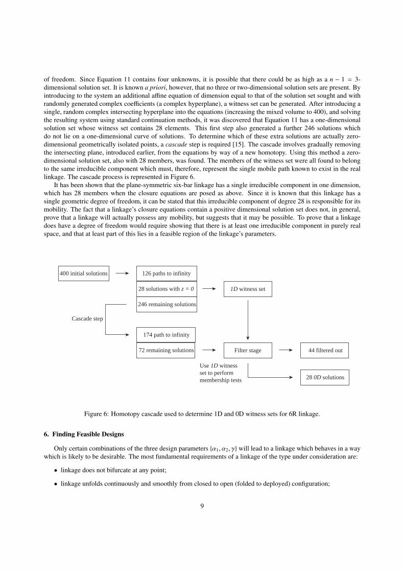
of freedom. Since Equation 11 contains four unknowns, it is possible that there could be as high as a n − 1 = 3-dimensional solution set. It is known a priori, however, that no three or two-dimensional solution sets are present. Byintroducing to the system an additional affine equation of dimension equal to that of the solution set sought and withrandomly generated complex coefficients (a complex hyperplane), a witness set can be generated. After introducing asingle, random complex intersecting hyperplane into the equations (increasing the mixed volume to 400), and solvingthe resulting system using standard continuation methods, it was discovered that Equation 11 has a one-dimensionalsolution set whose witness set contains 28 elements. This first step also generated a further 246 solutions whichdo not lie on a one-dimensional curve of solutions. To determine which of these extra solutions are actually zero-dimensional geometrically isolated points, a cascade step is required [15]. The cascade involves gradually removingthe intersecting plane, introduced earlier, from the equations by way of a new homotopy. Using this method a zero-dimensional solution set, also with 28 members, was found. The members of the witness set were all found to belongto the same irreducible component which must, therefore, represent the single mobile path known to exist in the reallinkage. The cascade process is represented in Figure 6.

It has been shown that the plane-symmetric six-bar linkage has a single irreducible component in one dimension,which has 28 members when the closure equations are posed as above. Since it is known that this linkage has asingle geometric degree of freedom, it can be stated that this irreducible component of degree 28 is responsible for itsmobility. The fact that a linkage’s closure equations contain a positive dimensional solution set does not, in general,prove that a linkage will actually possess any mobility, but suggests that it may be possible. To prove that a linkagedoes have a degree of freedom would require showing that there is at least one irreducible component in purely realspace, and that at least part of this lies in a feasible region of the linkage’s parameters.

400 initial solutions 126 paths to infinity

28 solutions with z = 0

246 remaining solutions

1D witness set

174 path to infinity

72 remaining solutions Filter stage 44 filtered out

28 0D solutions

Cascade step

Use 1D witnessset to performmembership tests

Figure 6: Homotopy cascade used to determine 1D and 0D witness sets for 6R linkage.

6. Finding Feasible Designs

Only certain combinations of the three design parameters {α1, α2, γ} will lead to a linkage which behaves in a waywhich is likely to be desirable. The most fundamental requirements of a linkage of the type under consideration are:

• linkage does not bifurcate at any point;

• linkage unfolds continuously and smoothly from closed to open (folded to deployed) configuration;

9

• hinge angles are allowed only to lie in the range spanned by the same hinge’s angle when deployed, and theangle when stowed;

• no two bars intersect during the unfolding process.

It has been observed that the satisfaction of the first three points ensures the satisfaction of the fourth, and so thisfourth point is not considered here.

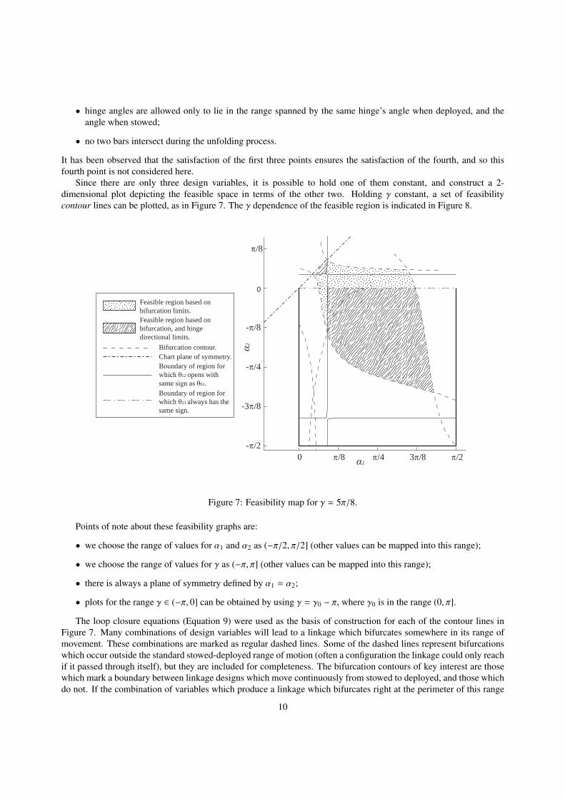
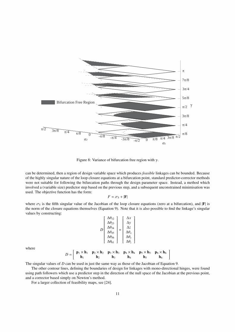
Since there are only three design variables, it is possible to hold one of them constant, and construct a 2-dimensional plot depicting the feasible space in terms of the other two. Holding γ constant, a set of feasibilitycontour lines can be plotted, as in Figure 7. The γ dependence of the feasible region is indicated in Figure 8.

0 �/8 �/4 3�/8 �/2-�/2

-3�/8

-�/4

-�/8

0

�/8

α1

α2

Feasible region based on bifurcation limits.Feasible region based on bifurcation, and hinge directional limits.

Bifurcation contour.Chart plane of symmetry.Boundary of region for which θ12 opens with same sign as θ61.Boundary of region for which θ23 always has thesame sign.

Figure 7: Feasibility map for γ = 5π/8.

Points of note about these feasibility graphs are:

• we choose the range of values for α1 and α2 as (−π/2, π/2] (other values can be mapped into this range);

• we choose the range of values for γ as (−π, π] (other values can be mapped into this range);

• there is always a plane of symmetry defined by α1 = α2;

• plots for the range γ ∈ (−π, 0] can be obtained by using γ = γ0 − π, where γ0 is in the range (0, π].

The loop closure equations (Equation 9) were used as the basis of construction for each of the contour lines inFigure 7. Many combinations of design variables will lead to a linkage which bifurcates somewhere in its range ofmovement. These combinations are marked as regular dashed lines. Some of the dashed lines represent bifurcationswhich occur outside the standard stowed-deployed range of motion (often a configuration the linkage could only reachif it passed through itself), but they are included for completeness. The bifurcation contours of key interest are thosewhich mark a boundary between linkage designs which move continuously from stowed to deployed, and those whichdo not. If the combination of variables which produce a linkage which bifurcates right at the perimeter of this range

10

0 �/8 �/4 3�/8 �/2-�/2-3�/8-�/4-�/80�/8�/43�/8�/2

�/8

�/4

3�/8

�/2

5�/8

3�/4

7�/8

�

γBifurcation Free Region

α2

α1

Figure 8: Variance of bifurcation free region with γ.

can be determined, then a region of design variable space which produces feasible linkages can be bounded. Becauseof the highly singular nature of the loop closure equations at a bifurcation point, standard predictor-corrector methodswere not suitable for following the bifurcation paths through the design parameter space. Instead, a method whichinvolved a (variable size) predictor step based on the previous step, and a subsequent unconstrained minimisation wasused. The objective function has the form:

F = σ5 + |F|

where σ5 is the fifth singular value of the Jacobian of the loop closure equations (zero at a bifurcation), and |F| isthe norm of the closure equations themselves (Equation 9). Note that it is also possible to find the linkage’s singularvalues by constructing:

D

∆θ12∆θ23∆θ34∆θ45∆θ56∆θ61

=

∆x∆y∆z∆θx

∆θy

∆θz

where

D =

[p1 × h1 p2 × h2 p3 × h3 p4 × h4 p5 × h5 p6 × h6

h1 h2 h3 h4 h5 h6

]The singular values of D can be used in just the same way as those of the Jacobian of Equation 9.

The other contour lines, defining the boundaries of design for linkages with mono-directional hinges, were foundusing path followers which use a predictor step in the direction of the null space of the Jacobian at the previous point,and a corrector based simply on Newton’s method.

For a larger collection of feasibility maps, see [24].

11

7. Simulating the Linkage’s Kinematics

A loop closure equation based on each of the linkage’s six hinge angles was derived in section 4. In this section,a similar equation is derived, but only in terms of two of the hinge angles. This equation will be referred to as acompatibility equation, as it ensures the compatibility of each half of the ring at the plane of symmetry. This is madepossible by way of the assumption that the linkage is always symmetric about the plane defined by hinges h6 and h3.This assumption directly forms the basis of the compatibility equation, which can be written as:

Φ =[(p6 − p3) × h6

]· h3 = 0. (12)

This equation can be written entirely in terms of the variable hinge angles θ61 and θ12 (as well as the fixed designparameters α1, α2 and γ). If one of the hinge angles, say θ61, is nominated as the driving, or input angle, then Equation12 can be used to find θ12 in terms of θ61; the other four hinge angles can then be found.

If the locations of hinges 1 and 2 (p1 and p2) are held fixed in space, then the locations of hinges 6 and 3 (p6 andp3) can be found by rotating their locations in the deployed configuration about unit hinge vectors h1 and h2. To rotatea vector v about a (unit) axis w by an angle θ:

v′ = (v · w)w + (v − (v · w)w) cos θ + v × w sin θ (13)

If the axis w passes through a point p, and the substitution u = v − p is made, then:

v′ = (u · w)w + (u − (u · w)w) cos θ + u × w sin θ + p (14)

Applying Equation 14 to the current problem for p1 and p2 gives:

p6 = (u1 · h1)h1 + (u1 − (u1 · h1)h1) cos θ61 + u1 × h1 sin θ61 + p1(0)

p3 = (u2 · h2)h2 + (u2 − (u2 · h2)h2) cos θ12 + u2 × h2 sin θ12 + p2(0)(15)

where u1 = p6(0) − p1(0) and u2 = p3(0) − p2(0). Hinge vectors h6 and h3 also change during the folding/unfoldingprocess. Applying Equation 13 to the problem of finding the hinge orientations gives:

h6 = (h6(0) · h1)h1 + (h6(0) − (h6(0) · h1)h1) cos θ61 + h6(0) × h1 sin θ61

h3 = (h3(0) · h2)h2 + (h3(0) − (h3(0) · h2)h2) cos θ12 + h3(0) × h2 sin θ12(16)

Assume that the bar connecting hinges 1 and 2 is fixed in space (i.e., the plane of symmetry moves). Since theposition of hinge 6 is being rotated about h1, it is possible to use Equation 16 to decompose h6 using:

a6 = (h6(0) · h1)h1

b6 = (h6(0) − (h6(0) · h1)h1)

c6 = h6(0) × h1

and thush6 = a6 + b6 cos θ61 + c6 sin θ61

h3 = a3 + b3 cos θ12 + c3 sin θ12

The positions of the hinges can also be parameterised as:

q6 = (u1 · h1)h1 + p1(0)

r6 = (u1 − (u1 · h1)h1)

s6 = u1 × h1

leading to:p6 = q6 + r6 cos θ61 + s6 sin θ61

p3 = q3 + r3 cos θ12 + s3 sin θ12

12

Substituting these forms into Equation 12, and collecting trigonometric terms leads to:

η0 + η1 cos θ12 + η2 sin θ12 + η3 sin θ12 cos θ12 + η4 cos2 θ12 + η5 sin2 θ12 = 0 (17)

where ηi can be expressed explicitly in terms of θ61 as well as a6,b6 . . . q6, r6 . . . . The process can just as easily bereversed to write Equation 17 in terms of θ61 with a6,b6 . . . q6, r6 . . . found by choosing a value of θ12. It can be shownthat in fact:

η3 = 0η4 = η5

If a new definition is made for the trigonometric terms:

sin θ12 =l

√1 + l2

(18)

then it can be shown that:

l =η1η2 ± (η0 + η4)

√η2

1 + η22 − (η0 + η4)2

(η0 − η2 + η4)(η0 + η2 + η4)

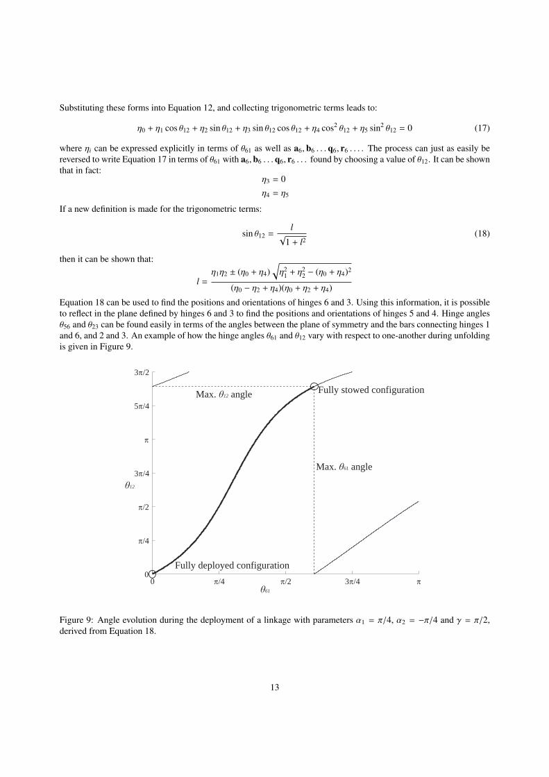
Equation 18 can be used to find the positions and orientations of hinges 6 and 3. Using this information, it is possibleto reflect in the plane defined by hinges 6 and 3 to find the positions and orientations of hinges 5 and 4. Hinge anglesθ56 and θ23 can be found easily in terms of the angles between the plane of symmetry and the bars connecting hinges 1and 6, and 2 and 3. An example of how the hinge angles θ61 and θ12 vary with respect to one-another during unfoldingis given in Figure 9.

0 �/4 �/2 3�/4 �0

�/4

�/2

3�/4

�

5�/4

3�/2

θ61

Max. θ61 angle

Max. θ12 angle Fully stowed configuration

Fully deployed configuration

θ12

Figure 9: Angle evolution during the deployment of a linkage with parameters α1 = π/4, α2 = −π/4 and γ = π/2,derived from Equation 18.

13

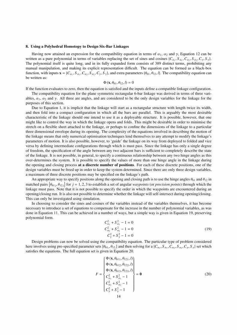
8. Using a Polyhedral Homotopy to Design Six-Bar Linkages

Having now attained an expression for the compatibility equation in terms of α1, α2 and γ, Equation 12 can bewritten as a pure polynomial in terms of variables replacing the set of sines and cosines {Cα1 , S α1 ,Cα2 , S α2 ,Cγ, S γ}.The polynomial itself is quite long, and in its fully expanded form consists of 389 distinct terms, prohibiting anymanual manipulation, and making its explicit representation difficult. The equation can be formed as a black-boxfunction, with inputs x = {Cα1 , S α1 ,Cα2 , S α2 ,Cγ, S γ}, and extra parameters {θ61, θ12, l}. The compatibility equation canbe written as:

Φ (x, θ61, θ12, l) = 0

If the function evaluates to zero, then the equation is satisfied and the inputs define a compatible linkage configuration.The compatibility equation for the plane symmetric rectangular 6-bar linkage was derived in terms of three vari-

ables, α1, α2 and γ. All three are angles, and are considered to be the only design variables for the linkage for thepurposes of this section.

Due to Equation 1, it is implicit that the linkage will start as a rectangular structure with length twice its width,and then fold into a compact configuration in which all the bars are parallel. This is arguably the most desirablecharacteristic of the linkage should one intend to use it as a deployable structure. It is possible, however, that onemight like to control the way in which the linkage opens and folds. This might be desirable in order to minimise thestretch on a flexible sheet attached to the linkage, or perhaps to confine the dimensions of the linkage to a particularthree dimensional envelope during its opening. The complexity of the equations involved in describing the motion ofthe linkage means that only numerical optimisation techniques lend themselves to any attempt to modify the linkage’sparameters of motion. It is also possible, however, to ‘guide’ the linkage on its way from deployed to folded and viceversa by defining intermediate configurations through which is must pass. Since the linkage has only a single degreeof freedom, the specification of the angle between any two adjacent bars is sufficient to completely describe the stateof the linkage. It is not possible, in general, to specify a continuous relationship between any two hinge angles as thisover-determines the system. It is possible to specify the values of more than one hinge angle in the linkage duringthe opening and closing process at a discrete number of positions. For each of these discrete positions, one of thedesign variables must be freed up in order to keep the system determined. Since there are only three design variables,a maximum of three discrete positions may be specified on the linkage’s path.

An appropriate way to specify positions along the opening and closing path is to use the hinge angles θ61 and θ12 inmatched pairs

{θ61 j, θ12 j

}for j = 1, 2, 3 to establish a set of angular waypoints (or precision points) through which the

linkage must pass. Note that it is not possible to specify the order in which the waypoints are encountered during anopening/closing run. It is also not possible to determine whether the linkage will self-intersect during opening/closing.This can only be investigated using simulation.

In choosing to consider the sines and cosines of the variables instead of the variables themselves, it has becomenecessary to introduce a set of equations to compensate for the increase in the number of polynomial variables, as wasdone in Equation 11. This can be achieved in a number of ways, but a simple way is given in Equation 19, preservingpolynomial form.

C2α1

+ S 2α1− 1 = 0

C2α2

+ S 2α2− 1 = 0

C2γ + S 2

γ − 1 = 0

(19)

Design problems can now be solved using the compatibility equation. The particular type of problem consideredhere involves using pre-specified parameter sets

{θ61i , θ12i

}and then solving for a {Cα1 , S α1 ,Cα2 , S α2 ,Cγ, S γ} set which

satisfies the equations. The full equation set is given in Equation 20.

F =

Φ (x, θ611, θ121, l)

Φ (x, θ612, θ122, l)

Φ (x, θ613, θ123, l)

C2α1

+ S 2α1− 1

C2α2

+ S 2α2− 1

C2γ + S 2

γ − 1

= 0 (20)

14

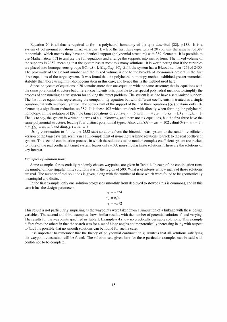
Equation 20 is all that is required to form a polyhedral homotopy of the type described [22], p.138. It is asystem of polynomial equations in six variables. Each of the first three equations of 20 contains the same set of 389monomials, which means they have an identical support (polynomial structure) with 389 elements. It is possible touse Mathematica [17] to analyse the full equations and arrange the supports into matrix form. The mixed volume ofthe supports is 2352, meaning that the system has at most this many solutions. It is worth noting that if the variablesare placed into homogeneous groups [{Cα1 , S α1 }, {Cα2 , S α2 }, {Cγ, S γ}], the system has a Bezout number [25] of 2400.The proximity of the Bezout number and the mixed volume is due to the breadth of monomials present in the firstthree equations of the target system. It was found that the polyhedral homotopy method exhibited greater numericalstability than those using multi-homogenisation in this case, and hence this is the method used here.

Since the system of equations in 20 contains more than one equation with the same structure; that is, equations withthe same polynomial structure but different coefficients, it is possible to use special polyhedral methods to simplify theprocess of constructing a start system for solving the target problem. The system is said to have a semi-mixed support.The first three equations, representing the compatibility equation but with different coefficients, is treated as a singleequation, but with multiplicity three. The convex hull of the support of the first three equations (Q1) contains only 102elements; a significant reduction on 389. It is these 102 which are dealt with directly when forming the polyhedralhomotopy. In the notation of [26], the target equations of 20 have n = 6 with r = 4 : k1 = 3, k2 = 1, k3 = 1, k4 = 1.That is to say, the system is written in terms of six unknowns, and there are six equations, but the first three have thesame polynomial structure, leaving four distinct polynomial types. Also, dim(Q1) = m1 = 102 , dim(Q2) = m2 = 3 ,dim(Q3) = m3 = 3 and dim(Q4) = m4 = 3.

Using continuation to follow the 2352 start solutions from the binomial start system to the random coefficientversion of the target system, results in a full complement of non-singular finite solutions to track to the real coefficientsystem. This second continuation process, in which the solutions to the random complex coefficient system are trackedto those of the real coefficient target system, leaves only ∼500 non-singular finite solutions. These are the solutions ofkey interest.

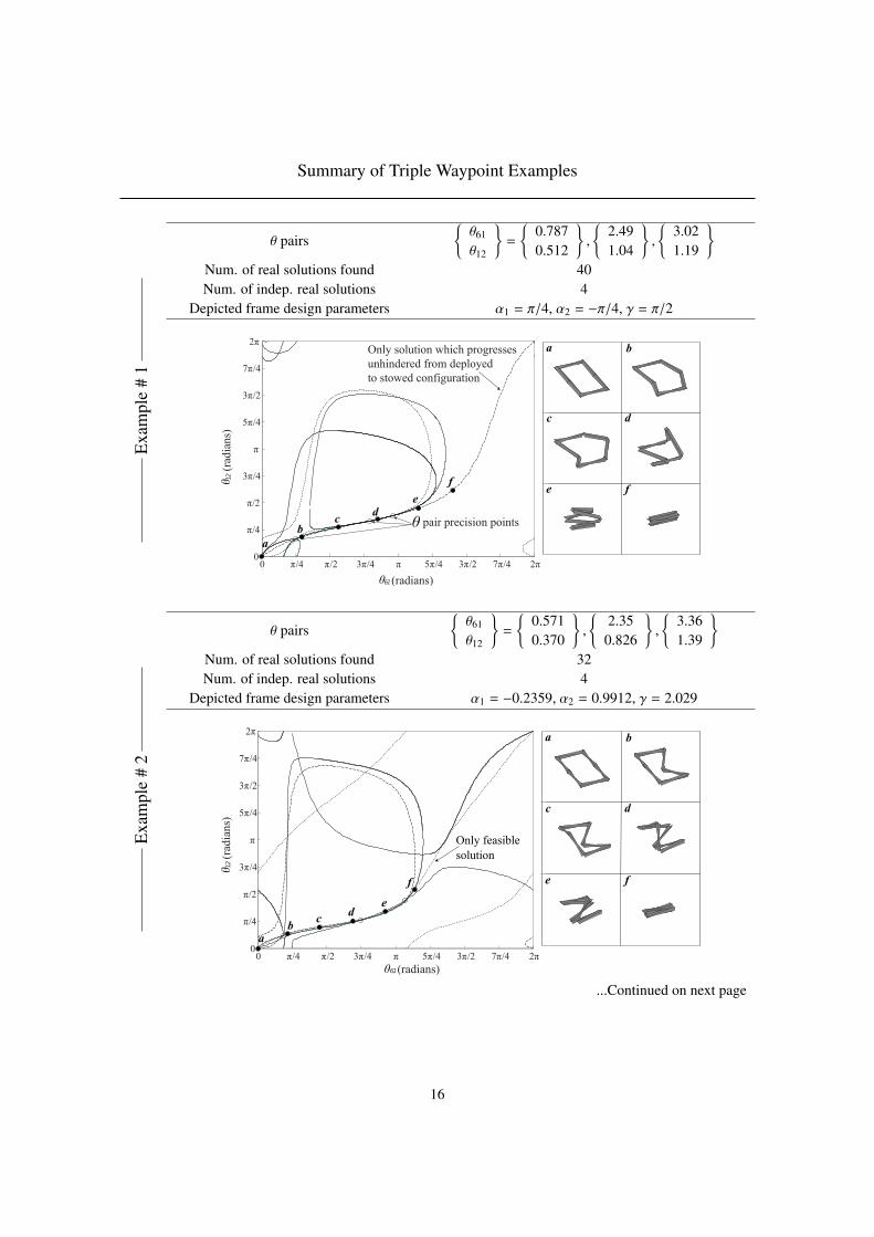
Examples of Solution Runs

Some examples for essentially randomly chosen waypoints are given in Table 1. In each of the continuation runs,the number of non-singular finite solutions was in the region of 500. What is of interest is how many of those solutionsare real. The number of real solutions is given, along with the number of these which were found to be geometricallymeaningful and distinct.

In the first example, only one solution progresses smoothly from deployed to stowed (this is common), and in thiscase it has the design parameters:

α1 = −π/4α2 = π/4γ = −π/2

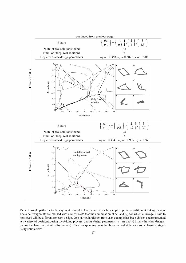
This result is not particularly surprising as the waypoints were taken from a simulation of a linkage with these designvariables. The second and third examples show similar results, with the number of potential solutions found varying.The results for the waypoints specified in Table 1, Example # 4 show no practically desirable solutions. This examplediffers from the others in that the search was for a set of hinge angles not monotonically increasing in θ12 with respectto θ61. It is possible that no smooth solutions can be found for such a case.

It is important to remember that the theory of polynomial continuation guarantees that all solutions satisfyingthe waypoint constraints will be found. The solution sets given here for these particular examples can be said withconfidence to be complete.

15

Summary of Triple Waypoint Examples

Exa

mpl

e#

1

θ pairs{θ61

θ12

}=

{0.7870.512

},

{2.491.04

},

{3.021.19

}Num. of real solutions found 40Num. of indep. real solutions 4

Depicted frame design parameters α1 = π/4, α2 = −π/4, γ = π/2

0 π/4 π/2 3π/4 π 5π/4 3π/2 7π/4 2π0

π/4

π/2

3π/4

π

5π/4

3π/2

7π/4

2π

pair precision points

Only solution which progressesunhindered from deployedto stowed configuration

61(radians)

12(radians)

θ

θ

θ

a b

c d

e f

ab

cd

e

f

Exa

mpl

e#

2

θ pairs{θ61

θ12

}=

{0.5710.370

},

{2.35

0.826

},

{3.361.39

}Num. of real solutions found 32Num. of indep. real solutions 4

Depicted frame design parameters α1 = −0.2359, α2 = 0.9912, γ = 2.029

0 π/4 π/2 3π/4 π 5π/4 3π/2 7π/4 2π0

π/4

π/2

3π/4

π

5π/4

3π/2

7π/4

2π

61(radians)

12(r

adia

ns)

θ

θ

a

a b

c d

e f

bc d

e

f

Only feasiblesolution

...Continued on next page

16

– continued from previous page

Exa

mpl

e#

3

θ pairs{θ61

θ12

}=

{1

0.5

},

{21

},

{3

1.5

}Num. of real solutions found 44Num. of indep. real solutions 7

Depicted frame design parameters α1 = −1.358, α2 = 0.5871, γ = 0.7206

0 π/4 π/2 3π/4 π 5π/4 3π/2 7π/4 2π0

π/4

π/2

3π/4

π

5π/4

3π/2

7π/4

2π

12(r

adia

ns)

61(radians)θ

θ

a b

c d

e f

ab

cd

ef

Only feasiblesolution

Exa

mpl

e#

4

θ pairs{θ61

θ12

}=

{1

0.5

},

{2

1.2

},

{3

0.7

}Num. of real solutions found 28Num. of indep. real solutions 3

Depicted frame design parameters α1 = −0.3941, α2 = −0.9053, γ = 1.560

0 π/4 π/2 3π/4 π 5π/4 3π/2 7π/4 2π0

π/4

π/2

3π/4

π

5π/4

3π/2

7π/4

2π

θ12(r

adia

ns)

θ61 (radians)

a b

c d

e f

ab

cd

e f

No fully stowedconfiguration

Table 1: Angle paths for triple waypoint examples. Each curve in each example represents a different linkage design.The θ pair waypoints are marked with circles. Note that the combination of θ61 and θ12 for which a linkage is said tobe stowed will be different for each design. One particular design from each example has been chosen and representedat a variety of positions during the folding process, and its design parameters (α1, α2 and γ) listed (the other designs’parameters have been omitted for brevity). The corresponding curve has been marked at the various deployment stagesusing solid circles.

17

9. Conclusion

The mobility of the plane symmetric 6R foldable ring over-constrained mechanism has been shown to manifestitself in the linkage’s closure equations as a single irreducible component in the one-dimensional solution set. Aset of ‘feasibility maps’ showing the regions in parameter space in which the 6R foldable ring exhibits desirablecharacteristics has been produced. Also, a method of designing such rings by specifying angular waypoints has beendemonstrated. It is hoped that these techniques, together, will provide a useful and practical way of designing planesymmetric, 6R foldable rings.

References

[1] R. Bricard, Memoire sur la theorie de l‘octaedre articule, Journal de mathematiques pures et appliquees 3 (1897) 113–148.[2] R. F. Crawford, J. M. Hedgepeth, P. R. Preiswerk, Spoked wheels to deploy large surfaces in space-weight estimates for solar arrays, Tech.

Rep. NASA-CR-2347; ARC-R-1004, NASA (1975).[3] Y. Chen, Z. You, T. Tarnai, Threefold-symmetric Bricard linkages for deployable structures, International Journal of Solids and Structures 42

(2004) 2287–2301.[4] Y. Chen, Z. You, Square deployable frames for space applications. part 1: theory, Journal of Aerospace Engineering 220 (2006) 347–354.[5] Y. Chen, Z. You, Square deployable frames for space applications. part 2: realization, Journal of Aerospace Engineering 221 (2006) 37–45.[6] Y. Chen, Design of structural mechanisms, Ph.D. thesis, University of Oxford (2003).[7] W. W. Gan, S. Pellegrino, Closed-loop deployable structures, in: 44th AIAA/ASME/ASCE/AHS Structures, Structural Dynamics, and Mate-

rials Conference, 2003.[8] K. Wohlhart, A new 6R space mechanism, in: Proceedings of the 7th World.Congress on the Theory of Machines and Mechanisms, Vol. 1,

Sevilla, Spain, 1987., pp. 193–198.[9] K. Wohlhart, The two types of the orthogonal Bricard linkage, Mechanism and Machine Theory 28 (1993) 809–817.

[10] L. Racila, M. Dahan, Spatial properties of Wohlhart symmetric mechanism, Meccanica 45 (2010) 153–165.[11] S. Pellegrino, C. Green, S. D. Guest, A. Watt, SAR advanced deployable structure, Tech. rep., University of Cambridge Department of

Engineering (2000).[12] W. W. Gan, S. Pellegrino, Kinematic bifurcations of closed-loop deployable frames, in: Proceedings of the 5th International Conference on

Computation of Shell and Spatial Structures, 2005.[13] W. W. Gan, S. Pellegrino, Numerical approach to the kinematic analysis of deployable structures forming a closed loop, Journal of Mechanical

Engineering Science 220 (C) (2006) 1045–1056.[14] Y. Chen, Z. You, Two-fold symmetrical 6R foldable frame and its bifurcations, International Journal of Solids and Structures 46 (2009)

4504–4514.[15] A. J. Sommese, J. Verschelde, Numerical homotopies to compute generic points on positive dimensional algebraic sets, Journal of Complexity

16 (2000) 572–602.[16] J. Baker, An analysis of the Bricard linkages, Mechanism and Machine Theory 15 (1980) 267–286.[17] Mathematica, Version 7.0, Wolfram Research, Inc., Champaign, Illinois, 2008.[18] F. Freudenstein, E. R. Maki, The creation of mechanisms according to kinematic structure and function, Environment and Planning B 6

(1979) 375–391.[19] A. J. Sommese, J. Verschelde, C. W. Wampler, Numerical decomposition of the solution sets of polynomial systems into irreducible compo-

nents, SIAM Journal of Numerical Analysis 38 (6) (2001) 2022–2046.[20] E. L. Allgower, K. Georg, Introduction to Numerical Continuation Methods, Society for Industrial and Applied Mathematics (SIAM), 2003.[21] A. Morgan, Solving Polynomial Systems Using Continuation for Engineering and Scientific Problems, Prentice-Hall, inc., 1987.[22] A. J. Sommese, C. W. Wampler, The Numerical Solution of Systems of Polynomials Arising in Engineering and Science, World Scientific,

2005.[23] T. Gao, T.-Y. Li, Mixed volume computation for semi-mixed systems, Discrete and Computational Geometry 29 (2) (2003) 257–277.[24] A. Viquerat, Polynomial continuation in the design of deployable structures, Ph.D. thesis, University of Cambridge (2011).[25] C. W. Wampler, A. P. Morgan, A. J. Sommese, Numerical continuation methods for solving polynomial systems arising in kinematics, Journal

of Mechanical Design 112 (1990) 59–68.[26] T. Y. Li, Handbook of Numerical Analysis, Vol. XI, North-Holland, 2003, Ch. Numerical Solution of Polynomial Systems by Homotopy

Continuation Methods, pp. 209–304.

18