A new time-ﬁnite-element implicit integration scheme for ...anderk5/papers/ImplicitIntegration.pdf · A new time-ﬁnite-element implicit integration scheme for multibody system

ARTICLE IN PRESS

www.elsevier.com/locate/cma

Comput. Methods Appl. Mech. Engrg. xxx (2005) xxx–xxx

A new time-finite-element implicit integration scheme formultibody system dynamics simulation

Mojtaba Oghbaei, Kurt S. Anderson *

Department of Mechanical, Aerospace, and Nuclear Engineering, Rensselaer Polytechnic Institute, Troy, New York 12180, United States

Received 22 June 2004; received in revised form 22 April 2005; accepted 22 April 2005

Abstract

When performing the dynamic simulation of stiff mechanical systems, implicit type integration schemes are usually required to pre-serve stability. This article presents a new implicit time integrator, which is a particular application of a novel state-time formulationrecently developed by the authors in a more general scope. The proposed scheme is constructed with the intent of benefitting fromthe accuracy and apparent robustness thus far achieved with this algorithm in an integration context. This is realized by first settingup the weighted residual equations for the system in a form associated with the application of a time marching integration scheme.The resulting algebraic equations are then solved, minimizing the error of integration time step in a generalized energy sense, allowingone to capture the stiff behavior of solution in an efficient manner. Examples are provided to show the proposed method performancewhen dealing with a stiff system.� 2005 Elsevier B.V. All rights reserved.

Keywords: Multibody dynamics; State-time formulation; Implicit integration scheme; Stiff mechanical systems

1. Introduction

Multibody systems (MBS) can be described as a collection of rigid and/or flexible bodies that are connected throughdifferent types of joints. Such systems can be found in various applications ranging widely from terrestrial vehicles, airand space applications to MEMS devices and biomechanical applications. Multibody dynamics, as a discipline describingthe dynamic behavior of such systems, plays a major role in the design and analysis of such systems. The benefits of cor-responding simulations and associated analysis are realized by increased reliability of theses systems through identificationof design defects, optimized design parameters, increased innovation, and/or reduction in the overall cost and time of thedevelopment cycle.

The state of MBS changes with time under the effect of applied forces and moments. When dynamic analysis of suchconstrained mechanical systems is desired, a set of often differential algebraic equations (DAE) describing the system equa-tions of motion must be set up and subsequently solved. Because time and accuracy are often both crucial in the simulationof the dynamic systems under consideration, an efficient time integration of these equations is of importance in the simu-lation of complex MBS. The traits of most interest in an underlying dynamic formulation and associated integrationscheme are the speed, accuracy, and robustness of the numerical algorithm. A variety of formulations and dynamic sim-ulation techniques have been developed which are sufficiently general to handle a wide range of MBS. Here we will limitour attention to the work which has most directly influenced the development of the procedure presented here.

0045-7825/$ - see front matter � 2005 Elsevier B.V. All rights reserved.

doi:10.1016/j.cma.2005.04.016

* Corresponding author.E-mail addresses: [email protected] (M. Oghbaei), [email protected] (K.S. Anderson).

mailto:[email protected]

mailto:[email protected]

2 M. Oghbaei, K.S. Anderson / Comput. Methods Appl. Mech. Engrg. xxx (2005) xxx–xxx

ARTICLE IN PRESS

The world is replete with systems where the stiffness or time scales associated with its components are sufficiently greatso that the resulting equations are termed ‘‘stiff’’ and exhibit stiff behavior. Stiffness may be produced by the physical prop-erties of a system or by the numerical techniques utilized to perform the simulation. For instance, MBSs that contain flex-ible parts, when discretized in the spatial domain, can lead to stiff modes with additional difficulties arising from time-dependence and nonlinearity. Very stiff springs, damping, or contact phenomena may also result in such behavior whichis often characterized by a combination of large overall motions and often localized high frequency components in the timedomain. In this case, the ratio of the maximum to minimum eigenvalues becomes large, and the effectiveness of explicitintegration methods is diminished due to the step size requirements needed to maintain integrator stability [1–4].

Negrut et al. [5] presented a state-space DAE solution framework that uses an associated implicit ODE code for numer-ical integration of a resulting reduced set of state-space ordinary differential equations. This concept was demonstrated byusing an implicit Runge–Kutta method in their methodology which has resulted in an L-stable, stiffly accurate implicitalgorithm. Additionally, a computational implementation of the implicit Park method, which is a linear combination ofthe second and the third order BDF (backward difference formula) method, is proposed in [6] for the simulation of stiffmechanical systems.

Multirate integration is another technique for the simulation of many physical systems where the solution componentscan be separated into two or more groups (fast and slow subsystems) with widely varying rates of change in temporal scale.A summary of the work done in this area may be found in [7–10]. Computational savings are realized because the Nord-sieck form of the Adams integrator does not have to evaluate and integrate the slower portions of the system with the samefrequency of the fast portions.

The focus of most of the algorithms developed so far has been based on either the direct use of traditional numericalmethods or a combination and/or modification thereof. Such methods solve for the system equations of motion in apoint-wise fashion, namely solving for unknown function values at the integration step boundary, and possibly at prede-termined interior points. Even though polynomial interpolation functions are often used to approximate the solution curve,the error control criteria as a rule can only be applied on the set of function approximated values on the boundaries of theintegration steps. However, there are other integration schemes proposed by some researchers which are based on aweighted residual development of a time marching algorithm. Some of these efforts are cited below.

Borri and Bottasso have discussed several features of finite elements in time domain with application on dynamic sys-tems. In [11], they presented two different weak formulations, i.e., Primal form (pure displacement formulation) and Mixedform (a two-field mixed formulation) to represent the dynamics of such systems. These formulations were based on theHamilton�s law of varying action, where the latter was a modification of the first by introducing the modified Hamiltonianfunction. The problem of rigid body dynamics was also considered in the context of Petrov–Galerkin mixed method for-mulation in [12]. In this work, the weak form for rigid body dynamics was derived using the linear and angular momentumbalance which was shown to be correspondent to the well-known Hamilton�s weak principle. This work was presented withthe idea of introducing an alternate integration scheme for the solution of governing dynamic equations. Recently it hasbeen shown by the same investigators that there is an intimate link existing between the finite element in time methods andthe popular implicit Runge–Kutta methods, with the only difference being in the choice of unknown variables [13,14].

Hughes and Hulbert [15,16] developed a space–time finite-element method for classical elastodynamics which employsthe discontinuous Galerkin method in time. Betsch and Steinmann have also developed several time-stepping finite-elementschemes which possess algorithmic energy conservation for the simulation of applications such as N-body problem, non-linear elastodynamics and mechanical systems with holonomic constraints [17–19]. In the first case, the time-steppingscheme is based on a Petrov–Galerkin finite-element method applied to the Hamiltonian formulation of the N-body prob-lem. For the second application, the discretization process utilizes the continuous Galerkin method applied to the Ham-iltonian formulation of semidiscrete nonlinear elastodynamics problem. A mixed Galerkin discretization method forindex 3 DAEs pertaining to finite dimensional mechanical systems with holonomic constraints is proposed in [19]. Themethod leads in a natural way to time-stepping algorithms that inherit major conservation properties of the underlyingconstrained Hamiltonian system, namely total energy and angular momentum.

These works are mostly based on Hamilton�s Principle which uses an energy-type approach in which the constraintforces interacting between adjacent bodies of a MBS will not appear explicitly in the equations of motion. This is an advan-tage of using indirect methods such as Lagrangian formulation over the other direct methods like Newton–Euler. However,on the negative side, they have tended to result in a dense and highly coupled system of nonlinear equations (for complexsystems) which generally do not lend themselves well to time and resource-effective computation.

One of the advantages of the proposed formulation relative to the conventional approaches is its ability to effectivelytreat and consider multiple time scales. Like multirate integration schemes, there exists the potential of simultaneouslyaccommodating multiple, grossly different time scales within a single simulation with this formalism. This can be accom-plished by allowing different suitable temporal interval sizes for each generalized coordinate or generalized force. It shouldbe noted that the main goal of this research [20] is to improve the state of the art in computationally efficient algorithms bycircumventing the time-marching nature of the traditional simulation techniques. This would provide the means to more

M. Oghbaei, K.S. Anderson / Comput. Methods Appl. Mech. Engrg. xxx (2005) xxx–xxx 3

ARTICLE IN PRESS

fully and effectively exploit anticipated massively parallel computing resources. However, in the case of current article, it isshown that the associated concept when utilized as a sequential algorithm can function well as an efficient and general impli-cit integration scheme.

The remainder of this article is organized as follows. The next section provides an outline of the proposed formulation,which is followed by the characteristics of the method. In Section 4, detailed simulation results of a stiff double pendulum isgiven along with comparison with other traditional implicit methods. At the end, some concluding remarks are made onthe use of this methodology for general multibody dynamics problems.

2. The proposed method

The new formulation is achieved by writing the weighted residual form of the full descriptor form of the governing equa-tions of a MBS [21] and then applying the Galerkin approximation in time domain over the current integration step. Theunderlying equations to be treated via this approach are the Newton–Euler equations, the Poisson�s kinematical equations[22], and the kinematic constraint equations for each body. Consider the MBS shown in Fig. 1(a) where the naming con-ventions for the variables associated with the free body diagram of a typical body B within this system are illustrated in part(b) of the same figure, and all are defined in the following.

It is worth mentioning here that as a result of such a temporal discretization, the system of differential equations is con-verted into a set of nonlinear algebraic equations. The use of the Newton–Euler formulation along with the parameteri-zation of orientation using Poisson�s kinematical equations result in a set of nonlinear algebraic equations, though oflarge dimension, is least coupled and at worst quadratic in system unknown variables.

Let us start with the weighted residual representation of the Euler�s equation associated with a representative body B inthe system. Euler�s equation can be written in general form as

X~M

B ¼Xk

~rkA �~F kA þXm

~rB�jm �~f mC þXl

T*

l ¼ ~~IB=B�

� N~aB þ N~xB � ~~IB=B�

� N~xB; ð1Þ

whereP

~MBrepresents all the moments applied on the body B, ~F kA is the kth applied force,~rkA is the kth position vector

from B* (the mass center of body B) to the application point of ~F kA, ~f mC is the mth unknown constraint force,~rB�jm is the

mth position vector from B* to application point (joint) of~f mC, ~T l is the lth applied concentrated moment, ~~IB=B�

is the iner-tia dyadic of body B with respect to B*, N~aB is the absolute angular acceleration of mass center of B, and N~xB is the absoluteangular velocity. The above equation can be written in indicial form as

eijhrkjCphF kp þ eijsrmjCnsfmn þ CqiT q ¼ I ijaj þ eijtxjI tlxl; ð2Þ

where eijh is the cyclic permutation operator, Cph are the elements of the direction cosine matrix, NCB from the local frame Bto the Newtonian reference frame N, and the other symbols are the scalar components of the vector quantities describedearlier. All indices except k and m vary from 1 to 3, while these two will depend on the number of applied and constraintforces acting on the body. Performing a weighted residual approach on the above ordinary differential equation results inthe following algebraic equation:

(a)

B

1 2

i

m

N

B*

B

Br

jiBr

*

ij2j

1j

mj

F1A

kAF

kAr

iCf

f1C

f2C

mCf

(b)

Fig. 1. Schematic of a multibody system.


ARTICLE IN PRESS

Cphx � eijhrkjF kp

Z 1

0

wxðtÞ � wrðtÞdt� �

þ Cqiy � T q

Z 1

0

wyðtÞ � wrðtÞdt� �

þ Cnsw � f mnt � eijsrmj

Z 1

0

wwðtÞ � utðtÞ � wrðtÞdt� �

� I ij qju _wuð1Þ � wrð1Þ � xjð0Þ � wrð0Þh i

� qju

Z 1

0

_wuðtÞ � _wrðtÞdt� �

� qju � qlv � eijtI tl

Z 1

0

_wuðtÞ � _wvðtÞ � wrðtÞdt� �

¼ 0 ð3Þ

in which the barred quantities represent the unknown nodal variables to be solved for, and w(t) and u(t) denote the tem-poral trial functions associated with the system state and force variables, respectively. The order of these functions are ingeneral different so that the Babuska–Brezzi condition [23] is satisfied. Variation of all the new sub indices in the aboveequation such as x, y, u and so forth depend on the order of trial functions.

Note that the equality ai ¼ _xi ¼ €qi is used where q exists mathematically, but not necessarily physically. Also, Eq. (3) isexpressed for a unit size temporal element (integration step) where in case of using Lagrange family of interpolating func-tions, it constitutes 3k quadratic algebraic equations and 9k + 3m(p + 1) + 3k unknown variables, with k and p being theorder of the trial functions associated with spatial and force variables respectively, and m is the number of geometricconstraints.

The next equation is the Newton�s second law of motion that is given below

~FB þ

Xm

~f mC ¼ mB€~rB ð4Þ

in which ~FB ¼

Pk~F kA, mB is the mass of body B, and~rB denotes the absolute displacement vector of the mass center in the

inertial reference frame. Applying the similar approach as described above on Eq. (4) results in the following algebraicequation where for simplicity the sub or superscript B is eliminated.

rij _wjð1Þ � wrð1Þ � _rið0Þ � wrð0Þn o

� rij

Z 1

0

_wjðtÞ � _wrðtÞdt

� 1

mF i

Z 1

0

wrðtÞdt þXm

f mk �Z 1

0

ukðtÞ � wkðtÞdt� �( )

¼ 0 i ¼ 1; 2; 3. ð5Þ

Eq. (5) constitutes 3k linear algebraic equations and introduces 3k additional unknowns per temporal element. All symbolsand indices reserve their meaning from before.

As the full descriptor formulation is used in the proposed scheme, another set of equation is needed to take the largerotational motion of MBS into consideration. There are several parameterizations available for describing the referenceframe orientations, such as the orientation angles (of which Euler�s angles are a subset), Euler�s parameters, and the directuse of direction cosines as rotation parameters. For the proposed methodology, it is realized that the last form of para-meterization results in the set of algebraic equations that are in the most desirable form. If the direction cosines are useddirectly as state variables, then the kinematical differential equations which relate the time derivative of the transformationmatrix to the angular velocity of the body are the Poisson�s kinematic equations given by

N _CB ¼ NCB � NxB

��

B; ð6Þ

where NxB�

� �B is the angular velocity cross-product matrix corresponding to the local body B reference frame and associ-

ated body-fixed basis vectors. This equation can be written in indicial form as

_Cil ¼ �emlkxkCim ð7Þin which, all symbols retain their definition from before. Eq. (8) shows the weighted residual representation of the Poisson�sequations over the current integration step which constitutes 9k quadratic algebraic equations and there are no additionalunknown variables introduced by them.

Ciln �Z 1

0

_wnðtÞwrðtÞdt þ Cimj � emlkqkp

Z 1

0

_wpðtÞ � wjðtÞ � wrðtÞdt� �

¼ 0. ð8Þ

Note that in this equation each element of the direction cosine matrix is treated as an independent variable and approx-imated in much the same manner as the other state variables. Also, in all the equations derived so far (i.e., Eqs. (3), (5), and(8)), the weighting functions are considered the same as the trial functions associated with the system state variables.

Fig. 2. Kinematic constraint relationships for body B and its neighbors.


ARTICLE IN PRESS

The last set of equations to be considered are the kinematic constraint equations. Consider again the body B with m

neighboring bodies as illustrated in Fig. 2. For each joint Ji, the velocity level of kinematic constraint equations can bewritten as

_~rB þ N _C

BrB�ji ¼ _~r

i þ N _Ciri�ji i ¼ 1; 2; . . . ;m ð9Þ

with their weighted residual representation given in Eq. (10) that form a linear set of equations.

rBtj

Z 1

0

_wjðtÞ � uzðtÞdt þ NCBtkm

Z 1

0

rB�ji k_wmðtÞ � uzðtÞdt � rits

Z 1

0

_wsðtÞ � uzðtÞdt

þ NCitln

Z 1

0

ri�ji l_wnðtÞ � uzðtÞdt ¼ 0 i ¼ 1; 2; . . . ;m. ð10Þ

This results in an additional 3m(p + 1) equations per current temporal element that if considered along with all the otherbodies� discretized equations will form a consistent number of equations and unknowns. As indicated earlier, the combi-nation of all discretized equations exhibits only quadratic nonlinearity in the nodal variables with a significant linear partas reiterated in compact form in Eq. (11).

A1q � qþ B1C � f þ D1qþ E1C ¼ R1;

A2r þ B2f ¼ R2;

A3C þ B3C � q ¼ R3;

A4r þ B4C ¼ R4;

ð11Þ

which are sorted based on Eqs. (3), (5), (8) and (10), respectively. The coefficient matrices as well as the right-hand residualsRi are known as soon as the system parameters, initial states, and initial guess are provided with these equations. Note thatthe underlined barred quantities are the matrix representation of each set of unknown nodal variables described earlier.This matrix of unknown variables may then be solved for by an appropriate nonlinear system solution scheme.

3. Characteristics of the method

When solving a matrix of initial value problems, one common approach is to convert the governing equations into thestate-space form as

y0 ¼ f ðt; yÞ yðt0Þ ¼ y0 ð12Þ

in which depending on whether the unknown function values at the terminal boundary of integration step are used, themethod is called explicit or implicit. Implicit methods tend to result in a set of nonlinear algebraic equations that needa Newton type method to solve for the unknown variables. In this sense, the proposed method is regarded as an implicittype integrator since at each integration step the evaluation requires the use of system state information at the terminalboundary of the temporal element. To achieve this a Newton-type method is applied on Eq. (11) to solve for unknownnodal variables.

Fig. 3. Tangent matrix structure for the stiff n-body pendulum. (a) The stiff n-body pendulum, (b) the traditional state-space method and (c) the proposedmethod.


ARTICLE IN PRESS

If the standard quadratic and linear Lagrange shape functions are used for spatial variables and constraint forces,respectively then there are two unknown barred quantities per each spatial variable namely the middle and the final nodesand two unknown barred quantities per each constraint force that are the initial and final nodes of the integration step.Once the Newton iteration converges at the current step, the boundary nodes will be updated and used as initial valuesfor the next integration step and the simulation marches forward temporally.

Due to the sparse structure and minimum degree of nonlinearity of the equations resulting from this formulation, themethod should perform well relative to traditional methods when applied to systems possessing a large number of general-ized coordinates and or kinematic constraints. Specifically, more traditional state-space type formulations yield systems ofsubstantially smaller dimension, but the associate equations are highly, often fully coupled, and extremely nonlinear. Insuch cases, the associated tangent matrix is heavily populated, expensive to produce, and even more expensive to decom-pose. Also, given the great level of nonlinearity associated with these approaches when applied to large complex systems,the number of iteration required for convergence of the method at each time step may be large. By comparison, the pro-posed formulation, though resulting in a larger set of equations, is in the least coupling form and produces the minimumdegree of nonlinearity. Generation of the associated tangent matrix is trivial and corresponding decomposition and solu-tion of the resulting system of equations at each iteration is relatively inexpensive.

For instance, let us consider a stiff n-body serial pendulum problem as shown in Fig. 3(a), where stiffness is introducedthrough the rotational springs and dampers mounted on the connecting joints. As the problem involves stiff modes, animplicit integrator is required for a stable numerical integration and as such it requires solving a system of nonlinear alge-braic equations. Fig. 3 demonstrates a comparison between the structure of the tangent matrix associated with the pro-posed formulation using linear-quadratic Lagrange element and a traditional state-space type formulation for thisproblem. The latter approach will produce a smaller set of equations while being highly nonlinear (nth order transcendentalnonlinearity) and heavily coupled. Hence, the lower part of the tangent matrix will be fully populated after linearization asshown in Fig. 3(b). Thus, for relatively large values of n the cost of decomposing and solving such system will be in theorder of Oðn3Þ for each iteration, while using the proposed method will result in OððbandwidthÞ2 � nÞ operations that is muchsmaller than the other. Moreover, as the number of bodies are increased, there will be additional diagonal blocks intro-duced to the sparse block diagonal structure of the system tangent matrix and the bandwidth remains constant.

Given the at-worst quadratic nonlinearity of the resulting equations in this method, convergence has been thus farshown to be rapid. Additionally, there has been a great deal of literature presenting efficient (and parallelizable) solutionmethods for the system of large scale linear and quadratic equations which can also be exploited within this formulation[24,25]. Hence, the proposed method can potentially serve as an efficient and robust time integration scheme particularlywhen dealing with large complex multibody systems.

3.1. Stability analysis

Ideally, one would desire that a general argument be made on the properties of a numerical method employed for thesolution of a class of differential equations. This will be too complicated in general, as for instance in the case of nonlinearproblems the behavior of the system is dependent on the particular solution trajectory considered (i.e., the initial state). As


ARTICLE IN PRESS

such, usually the characteristics of a method is tested to capture the essential properties of a class of differential equations,termed as the test equation. Stability analysis is performed by checking the variation of the spectral radius q of the ampli-fication or transition matrix (the matrix A in Eq. (13)) derived for the test equation. The spectral radius of this matrix,which maps the initial (known) state of the system into the unknown state vector, is the largest absolute value of its eigen-values. To ensure unconditional stability, this quantity must not exceed unity. Indeed, this is taken from the following fact.The absolute stability requirement suggests that since for all stable test equations jy(tn)j 6 jy(tn�1)j, an (A-stable) discret-ization method should behave in the same fashion, as well.

yn ¼ Ayn�1 q ¼ max jkij. ð13Þ

Let us consider the matrix form of the test equation, i.e., y 0 = A2·2y which is the state-space representation of a secondorder ODE. To check for the stability behavior of the proposed formulation, we apply the suggested discretization schemeon the following standard linear 1DOF oscillator (spring–mass–damper) and analyze the variation of its spectral radius.

€xþ 2fxn _xþ x2nx ¼ f ðtÞ. ð14Þ

Utilizing the family of quadratic Lagrange shape functions on an integration step [tn�1, tn], with h being the length of thedomain h = tn � tn�1, results in a set of two linear equations and two unknowns. These variables are �x2 and �x3 which denotethe unknown nodal variables associated with the middle node t ¼ tn�1þtn

2, and boundary node t = tn. It should be noted that

in general once these nodal variables are known, they are substituted in the approximate relations and some post-process-ing calculations provide the velocity information throughout the domain yielding the initial condition for the next incre-ment. Manipulating these equations and writing them in matrix form result in

f11ðh; f;xnÞ f12ðh; f;xnÞf21ðh; f;xnÞ f22ðh; f;xnÞ

� ��x2�x3

� �¼

x0v0

� �ð15Þ

f(t) is eliminated as it does not affect the analysis. The inverse of the coefficient matrix in Eq. (15) forms the amplificationmatrix for the proposed method which obviously is a function of h, f and xn.

A simple script was written to check the variation of the absolute values of the eigenvalues of the amplification matrix.This was made possible by changing each parameter present in the matrix A, namely, h, f, xn for quite a large range. It wasrealized that one of the absolute eigenvalues of this matrix, jk1j always lies between 0 and 0.75 and the other, jk2j isbounded by �0.25. Therefore, the spectral radius of this system remains always smaller than unity for all combinationsof mass, spring and damper coefficients and the interval size of h. To reassure about these results, the two equations jkij = a

i = 1,2 were also solved in Maple� for h given a large range of variation on f and xn, and for different values of 0 6 a 6 1.There was no solution found for h if a was chosen greater than the above values (0.75 and 0.25, respectively) for each of thecases i = 1,2, which confirms the results mentioned above.

As an example, an underdamped system with the physical parameters m = 1, c = 0.4, k = 0.16 (all units are SI) was con-sidered which produces the natural frequency of xn ¼

ffiffiffiffiffiffiffiffiffik=m

p¼ 0:4 and the damping coefficient f ¼ c=ccr ¼ c=2

ffiffiffiffiffiffimk

p¼ 0:5.

The eigenvalues of the amplification matrix (using 3-noded Lagrange element) were plotted as a function of h which can beseen in Fig. 4. In this plot, the upper curve (plotted as solid line) determines the variations of the spectral radius.

Similar analysis was repeated for the case of cubic and quartic families of Lagrange shape functions, where it wasnoticed that as the order of shape functions is increased, the upper bound of spectral radii decreases. For the above

10-1 100 101 1020

0.1

0.2

0.3

0.4

0.5

0.6

0.7

0.8Eigenvalues versus the integration step size, h

h

Eig

enva

lues

Lambda-1

Lambda-2

Fig. 4. Eigenvalues of the amplification matrix (quadratic Lagrange element).

0

0.1

0.2

0.3

0.4

0.5

0.6

0.7

0.8

10-1 100 101 102

h

Spe

ctra

l Rad

ius

Quadratic element

Cubic element

Quartic element

Spectral radius versus the integration step size, h

Fig. 5. Spectral radii of the amplification matrices.


ARTICLE IN PRESS

mentioned example, the variation of spectral radii for all these cases, i.e., using quadratic, cubic and quartic shape func-tions are shown in Fig. 5.

As a final note, the stability analysis of a simple nonlinear system was also considered for a number of initial conditionsand initial guesses. Nonlinearity was introduced to the above 1DOF oscillator by adding a cubic stiffness term k2x

3 whichconverts the linear system into the well-known Duffing nonlinear oscillator

€xþ 2fxn _xþ x2nxþ x2

NLx3 ¼ f ðtÞ; ð16Þ

where xNL ¼ffiffiffiffiffiffiffiffiffiffik2=m

p. Discretizing equation (16) using the proposed method and via the 3-noded Lagrange element results

in a nonlinear algebraic equation which after linearization about the current iteration point takes the form

g11ðh; f;xn; x0; v0;�xi�12 ;�xi�1

3 Þ g12ðh; f;xn; x0; v0;�xi�12 ;�xi�1

3 Þg21ðh; f;xn; x0; v0;�xi�1

2 ;�xi�13 Þ g22ðh; f;xn; x0; v0;�xi�1

2 ;�xi�13 Þ

" #d�xi2d�xi3

� �¼ Residualf g. ð17Þ

In this equation, x0 and v0 are the initial state, �xi�12 and �xi�1

3 are the updated initial guess from the (i � 1)th iteration, and d�xi2and d�xi3 are the updated differential change in unknown nodal variables at the current ith iteration. Thus, as indicatedabove the behavior of the system is dependent on the particular solution trajectory considered. Similar analysis was carriedout for this system where by altering the values of h, f, xn and wNL the range of variation of the amplification matrix eigen-values were examined. In this case, it was also noticed that the spectral radius of the amplification matrix and associatedwith the quadratic Lagrange element is bounded by 0.75. This result was verified by altering the values of initial states andguesses in several cases.

In the following section, an example is presented to indicate how the proposed method can be used as an implicit typeintegration scheme for a stiff dynamic system simulation.

4. Example: Stiff double pendulum

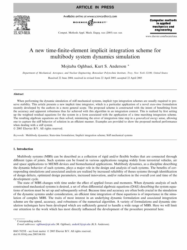
As a simple nonlinear example, consider the double pendulum depicted in Fig. 6. This system was selected because it iseasy to understand, demonstrates the accuracy and other characteristics of the method, and is an accepted test case avail-able in the literature [5]. Being that as it may, this problem will not perform well in assessing simulation speed and com-putational cost relative to state-space methods because as pointed out in Section 3, these methods will in this instance yielda heavily populated tangent matrix of dimension 4 · 4, whereas the formulation presented here will produce a bandedmatrix of dimension 28 · 28. Dynamic simulation results for this system are given based on different families of shape func-tions that are selected to interpolate the time history of state variables and constraint forces for the simulation period.Through simulation results, it is shown how this scheme can capture stiff behavior in the solution, with discussion providedon the characteristics and selection of the preferred family of shape functions.

4.1. System parameters

Stiffness is induced by properly selecting the constants of rotational spring/damper actuator acting on the joints. Thesame system parameters as given in [5] are chosen here which are: m1 = 3 and m2 = 0.3 masses of pendulums, l1 = 2

1q

2q

111 ,, lIm

222 ,, lIm

g

11, ck

22 , ck

x

y

Fig. 6. Stiff double pendulum.


ARTICLE IN PRESS

and l2 = 3 lengths of pendulums, k1 = 400, k2 = 3 · 105 and c1 = 15, c2 = 5 · 104 rotational springs and dampers coeffi-cients, respectively. All units are in SI. The zero tension angles for the two springs are q01 ¼ 0 and q02 ¼ p=2 and the initialconditions are q10 ¼ p=2; q20 ¼ 5p=12 and _q10 ¼ 0, _q20 ¼ 10. What makes this 2DOF system stiff is the dominant eigenvalueat the initial state which has a very small real part of the order �105.

Plots presented over the next pages provide representative results associated with the 2 s simulation of this pendulum viathe proposed formulation (hereafter referred to as ST), the BDF method, as well as the MATLAB� ODE15s solver that isspecifically written for the temporal integration of stiff systems. ODE15s is a variable order and a variable step size solverbased on the numerical differentiation formulas (NDFs). Optionally, the backward differentiation formulas (BDFs, alsoknown as Gear�s method) may also be utilized. It can use each of these formulas with a maximum order of accuracy of 5.

4.2. Lagrange family of shape functions

As indicated previously, the order of the polynomial interpolating functions associated with spatial variables and con-straint forces can and should be different from each other to satisfy the Babuska–Brezzi condition. This in many casesrequires the use of lower order interpolation functions for the force-type variables than for the spatial variables. The plots,which are presented in Fig. 7 show the time history of the angle q1 and angular velocity x1 using linear quadratic (LQ) (i.e.linear interpolation functions are used for the constraint force variables while quadratic interpolation functions for the spa-tial variables) and quadratic–cubic (QC) Lagrange shape functions and 75 integration steps. Note that there is a small sub-figure in each of the plots associated with angular velocity via the methods used throughout this article. This is to magnifythe region showing that there is an initial stiff behavior in the angular velocity as well as to indicate how well each method isable to capture it. The plots correspondent to each of the ST and ODE15s results are superimposed onto the same set ofaxes for better comparison.

In these plots, the ST solutions are obtained using 75 equally spaced intervals in the simulation period, while the resultsfrom Matlab ODE15s are generated using a variable step-size scheme. This is due to the fact that if this equal step-sizeinterval is prescribed to the ODE15s integrator, then it will just pass over the stiff behavior without capturing the initialrapid change in the angular velocity. Additionally, the proposed method was also tested with a variable step-size schemewhich demonstrated that it did capture the initial stiff part of the curve as well as maintaining the overall macro-behavior ofthe solution curve.

Comparison of the plots given in Fig. 7 shows graphically how the solution accuracy is improved through a p-typerefinement both in position and velocity level. Simulations are also run using different number of integration steps to pro-vide a measure/indicator of how error improves for both the LQ and QC cases. Fig. 8 illustrates the error analysis of thetwo above classes of shape functions used in the simulation of this problem. In this study, the same error assessment

method as presented in [5], i.e. the maximum error D(n) and the average trajectory error DðnÞ

are adopted, specifically

DðnÞ ¼ max16i6n

Di DðnÞ ¼ 1

nkDik2. ð18Þ

The error Di at time ti is defined as Di = jEi � eij, where Ei is the reference solution and ei is the simulation results obtainedusing selected number of integration steps, n, both at time ti. The grid points of the simulation interval are denoted bytinit = t1 < t2 < � � � < tn = tend. So, the reference solution is obtained first by applying a tight tolerance on the Matlab

0 0.2 0.4 0.6 0.8 1 1.2 1.4 1.6 1.8 2-1

-0.5

0

0.5

1

1.5

2Solution curve based on the proposed method & ODE15s solver: q1 vs. t, n=75

t (sec)

q1 (

rad)

0 0.2 0.4 0.6 0.8 1 1.2 1.4 1.6 1.8 2-1

-0.5

0

0.5

1

1.5


t (sec)

q1 (

rad)

0 0.2 0.4 0.6 0.8 1 1.2 1.4 1.6 1.8 2-10

-8

-6

-4

-2

0

2

4

6

8Solution curve based on the proposed method & ODE15s solver: w1 vs. t, n=75

t (sec)

w1

(rad

/sec

)

ODE15s Sol.Time FEM Sol.


-2 0 2 4

x 10-3

-0.4

-0.2

0

Stiff behavior

0 0.2 0.4 0.6 0.8 1 1.2 1.4 1.6 1.8 2-10

-8

-6

-4

-2

0

2

4

6


t (sec)

w1

(rad

/sec

)


-2 0 2 4

x 10-3

-0.4

-0.2

0Stiff behavior

(a) (b)

(c) (d)


Fig. 7. Simulation results of the stiff double pendulum, n = 75. (a) Angle q1 vs. t LQ interpolation, (b) angle q1 vs. t QC interpolation, (c) angular velocityw1 vs. t LQ interpolation and (d) angular velocity, w1 vs. t QC interpolation.

101

102

103

10-7

10-6

10-5

10-4

10-3

10-2

Average trajectory error for Q1 vs. Number of integration steps n

n

||Del

ta-Q

1|| 2/n

LQ shape functionsQC shape functions

LQ shape functionsQC shape functions

Average slope over thespecified range, S

SQC

=2.58

SLQ

=1.50

101

102

103

10-5

10-4

10-3

10-2

10-1

Average trajectory error for W1 vs. Number of integration steps n

n

||Del

ta-W

1|| 2/n

(a) (b)

Fig. 8. Average trajectory error in q1 and w1 for both LQ and QC cases. (a) Average trajectory error in the angle q1 and (b) average trajectory error in theangular velocity w1.


ARTICLE IN PRESS

ODE15s solver and then all the results are compared against them to find the maximum grid-point error and the averagetrajectory error per simulation period. The absolute and relative tolerances for the reference solution is set to 10�8.

These results are also tabulated in Table 1 for more convenient reference. Inspection of the numerics presented here indi-cates that the method exhibits a super-linear performance of 1.50 (that is the error decreases as (1/n)1.50) when using the

Table 1Average trajectory error as a function of number of integration steps

# of integration steps (n) 29 47 75 126 219 384 678

DðnÞq1

(LQ) 0.0096 0.0048 0.0024 0.0011 4.74e�4 2.04e�4 8.68e�5

DðnÞq1

(QC) 5.35e�4 1.43e�4 4.04e�5 1.01e�5 2.35e�6 5.53e�7 1.70e�7

DðnÞx1

(LQ) 0.0862 0.0406 0.0197 0.0089 0.0039 0.0016 6.94e�4

DðnÞx1

(QC) 0.0048 0.0013 3.54e�4 8.96e�5 2.50e�5 1.43e�5 1.30e�5


ARTICLE IN PRESS

linear-quadratic interpolation set, and super-quadratic performance of 2.58 for the quadratic–cubic interpolation set. Theaccuracy of the approach thus appears to be influenced by the lower order of the force-associated interpolating functions.

4.3. Combination of Lagrange–Hermite family of shape functions

Hermite family of interpolating functions along with the Lagrange shape functions are also used for the parametrizationof equations. In Hermite interpolation both function values and its derivatives of various order can be interpolated. Sincethe approximation is smooth in the element interior, interpolation of derivatives is considered for the nodes on the bound-aries of elements to ensure that the derivative of the interpolant is continuous across the interface. Since both position andvelocity level of the system state variables are present in the ST formulation, Hermite interpolating function would seem tobe a proper choice for continuous approximation of velocity type variables.

The idea here is to interpolate the spatial variables using Hermite shape functions and the constraint forces usingLagrange interpolation. Note that the former parametrization cannot be used for constraint forces since there is no infor-mation available on their derivative data. It is realized that to avoid the spurious modes in the system, a Lagrange shapefunction of at least two order in degree less than the Hermite shape function should be used, otherwise the system tangentmatrix becomes singular. Fig. 9 demonstrates the same simulation period for the stiff double pendulum using the combi-nation of the Lagrange and Hermite shape functions. In an effort to conserve space, only two representative results aregiven where the left plot is using the linear Lagrange–cubic Hermite element and the right plot is using quadraticLagrange–quartic Hermite element.

It is observed that the velocity level information of system state variables is not interpolated so well as the similar casewhere only the Lagrange shape functions were used. This is due to the fact that the system of equations are now moreconstrained and these constraints are not only on the system state variables but on their derivatives as well. Indeed, in thiscase at the end of each integration step, both the state variables and their derivatives are dictated to the system and con-sidered as unchangeable initial conditions for the next integration step. So, the Newton iterate does its best to minimize theerror over the current integration step in an average sense and this is what is exactly observed from the results if any por-tion of the solution is zoomed in. However, since the initial values are not allowed to change (due to the use of Hermiteshape function on spatial variables), the system has to balance the unknown nodal variables at the terminal boundary ofeach integration step in order to minimize the energy error norm. Thus, any offset in the initial position and velocity (that isdue to the error from the previous step) gets boosted in the current step and this accumulates as the simulation moves for-ward in time.

0 0.2 0.4 0.6 0.8 1 1.2 1.4 1.6 1.8 2-1

-0.5

0

0.5

1

1.5


t (sec)

q1 (

rad)

0 0.2 0.4 0.6 0.8 1 1.2 1.4 1.6 1.8 2-10

-8

-6

-4

-2

0

2

4

6


t (sec)

w1

(rad

/sec

)



-2 0 2 4

x 10-3

-0.4

-0.2

0Stiff behavior

(a) (b)

Fig. 9. Simulation results of the stiff double pendulum, n = 75. (a) angle q1 vs. t L1H3 interpolation and (b) angular velocity, w1 vs. t L2H4 interpolation.


ARTICLE IN PRESS

It is concluded through some test cases that overall the use of Lagrange interpolation is a better choice than the com-bination of Lagrange–Hermite shape functions. In the subsequent sections, comparisons are made between the results fromLagrange family of shape functions and the results presented in [5], as well as the results from a second order traditionalBDF method.

4.4. Comparison of results

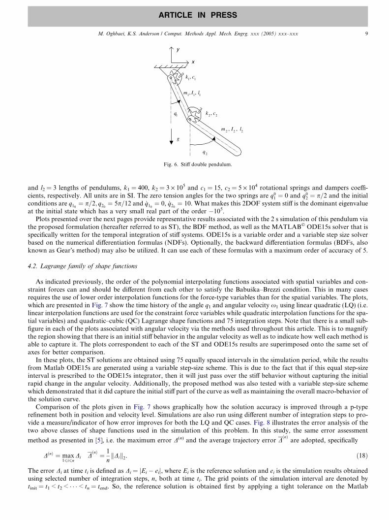
An implicit Runge–Kutta method for dynamic simulation of MBS is presented in [5]. The article presents a DAE reduc-tion process into the state-space ordinary differential equations (SSODE) through the generalized coordinate partitioningmethod [26]. In Table II of this article [5], the results of error analysis for the 2 s simulation of the problem at hand aretabulated and in Table III a comparison between the number of integration steps required to fulfill some tolerances isgiven. As shown above, the same number of integration steps are also taken for this problem using the described formu-lation. Fig. 10 shows a comparison between the results from ST QC-Lagrange shape functions and the results given inTable II of the above article.

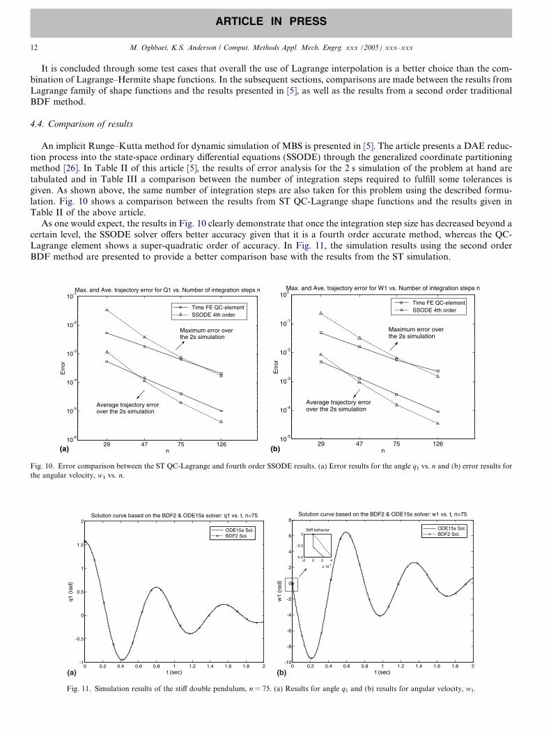
As one would expect, the results in Fig. 10 clearly demonstrate that once the integration step size has decreased beyond acertain level, the SSODE solver offers better accuracy given that it is a fourth order accurate method, whereas the QC-Lagrange element shows a super-quadratic order of accuracy. In Fig. 11, the simulation results using the second orderBDF method are presented to provide a better comparison base with the results from the ST simulation.

29 47 75 12610

-6

10-5

10-4

10-3

10-2

10-1Max. and Ave. trajectory error for Q1 vs. Number of integration steps n

n

Err

or

Maximum error overthe 2s simulation

Average trajectory error over the 2s simulation

Time FE QC-elementSSODE 4th order

29 47 75 12610

-5

10-4

10-3

10-2

10-1

100Max. and Ave. trajectory error for W1 vs. Number of integration steps n

n

Err

or

Maximum error overthe 2s simulation

Average trajectory error over the 2s simulation

(a) (b)

Time FE QC-elementSSODE 4th order

Fig. 10. Error comparison between the ST QC-Lagrange and fourth order SSODE results. (a) Error results for the angle q1 vs. n and (b) error results forthe angular velocity, w1 vs. n.

0 0.2 0.4 0.6 0.8 1 1.2 1.4 1.6 1.8 2-1

-0.5

0

0.5

1

1.5

2Solution curve based on the BDF2 & ODE15s solver: q1 vs. t, n=75

t (sec)

q1 (

rad)

0 0.2 0.4 0.6 0.8 1 1.2 1.4 1.6 1.8 2-10

-8

-6

-4

-2

0

2

4

6

8Solution curve based on the BDF2 & ODE15s solver: w1 vs. t, n=75

t (sec)

w1

(rad

)

ODE15s Sol.BDF2 Sol.

ODE15s Sol.BDF2 Sol.

-2 0 2 4

x 10-3

-0.4

-0.2

0Stiff behavior

(a) (b)

Fig. 11. Simulation results of the stiff double pendulum, n = 75. (a) Results for angle q1 and (b) results for angular velocity, w1.

0 0.001 0.002 0.003 0.004 0.005 0.006 0.007 0.008 0.009 0.01-1

-0.9

-0.8

-0.7

-0.6

-0.5

-0.4

-0.3

-0.2

-0.1


t (sec)

w1

(rad

/sec

)


The initial 0.01 sec of simulation using ODE15s and T-FEM LQ-element

0 0.001 0.002 0.003 0.004 0.005 0.006 0.007 0.008 0.009 0.01-1

-0.9

-0.8

-0.7

-0.6

-0.5

-0.4

-0.3

-0.2

-0.1


t (sec)

w1

(rad

/sec

)


The initial 0.01 sec of simulation using ODE15s and T-FEM QC-element

0 0.001 0.002 0.003 0.004 0.005 0.006 0.007 0.008 0.009 0.01-1

-0.9

-0.8

-0.7

-0.6

-0.5

-0.4

-0.3

-0.2

-0.1

0Solution curve based on the BDF2 & ODE45 solver: w1 vs. t, n=75

t (sec)

w1

(rad

/sec

)

ODE15s Sol.BDF2 Solution

The initial 0.01 secof simulation usingODE15s and BDF2

(a) (b)

(c)

Fig. 12. Capturing the stiff behavior via ST formulation. (a) LQ interpolation, (b) QC interpolation and (c) BDF2.


ARTICLE IN PRESS

Comparison of these plots with those presented in Fig. 7 shows that the results from BDF2 method are more accuratethan the ones from LQ-Lagrange element and slightly less accurate than the ones with QC-Lagrange element. This isexpected since the BDF2 is a second order method while the other two have super-linear and super-quadratic accuracy,respectively. Also, as indicated above the linear and angular velocity of the two bodies are approximated using Lagrangeshape functions which are of one degree less than the shape functions used for position coordinates and rotation angles.This is another source of reduced accuracy in the calculations per each integration step. Being that as it may, it is observedthat integration scheme based on the presented method shows better performance in capturing the region of solutionaround the stiff behavior. This is illustrated in Fig. 12, where plots are obtained by zooming in on the initial stiff behaviorof angular velocity curve of the simulations considered so far. Note that all methods perform the simulation with the sameconstant step size for integration.

5. Conclusion

When performing dynamic simulation of mechanical systems, a system of often differential algebraic equations must besolved at the current time step for the system state derivatives, which should be temporally integrated. The results fromcurrent integration step are then used to update the system state and the process repeats as the simulation marches sequen-tially forward in time.

By applying the proposed time-finite element (a.k.a. state-time [20]) methodology on the current temporal integrationstep and running the simulation in a sequential manner, it is shown that the method has the potential of acting as an effi-


ARTICLE IN PRESS

cient implicit integration scheme relative to more traditional state-space schemes for multibody systems with large numbersof degrees of freedom. This formulation will not be advantageous when dealing with simple mechanical systems, since itresults in a large set of equations and increased numerical effort. However, for sufficiently general and complex systemswhere there is a large set of equations and constraints, this method should offer particular advantage relative to traditionalmethods as the resulting system of equations exhibit at worst quadratic nonlinearity, and minimum degree of coupling.This results in a large but sparse system tangent matrix which is trivial to construct, and inexpensive to decompose andsolve. Additionally, the method becomes significantly beneficial when some or all constraint forces are explicitly neededfor the purpose of design/optimization and/or modeling of contact friction.

In this investigation, only the polynomial interpolating functions are utilized in the test cases presented. However, thereare other classes of approximating techniques such as compactly supported wavelet bases that have been shown to be apowerful numerical tool for the fast and accurate solution of partial differential equations occurring in various branchesof science and engineering. Their well-known multiresolution capability and localization properties can also be potentiallyused within this formulation which shows great promise when dealing with dynamic simulation of complex multibody sys-tems, particularly as it relates to capturing stiff behavior.

Acknowledgments

Support for this work has been provided by National Science Foundation (NSF) under the Award No. CMS-0219734and is gratefully appreciated. Also, the authors appreciate Mr. John Evans, one of URP students in the research group,who has contributed for some test cases.

References

[1] M. Schaub, B. Simeon, Automatic h-scaling for the efficient time integration of stiff mechanical systems, Multibody Syst. Dyn. J. 8 (2002) 329–345.[2] M. Schaub, B. Simeon, Blended Lobatto methods in multibody dynamics, ZAMM J. Appl. Math. Mech. 83 (10) (2003) 720–728.[3] J. Meijaard, Application of Runge–Kutta–Rosenbrock methods to the analysis of flexible multibody systems, Multibody Syst. Dyn. J. 10 (2003) 263–

288.[4] S. Chen, D.A. Tortorelli, An energy-conserving and filtering method for stiff nonlinear multibody dynamics, Multibody Syst. Dyn. J. 10 (2003) 341–

362.[5] D. Negrut, E.J. Haug, H.C. German, An implicit Runge–Kutta method for integration of differential algebraic equations of multibody dynamics,

Numer. Alg. 9 (2003) 121–142.[6] D. Pogorelov, Differential-algebraic equations in multibody system modelling, Multibody Syst. Dyn. J. 19 (1998) 183–194.[7] S. Kim, E.J. Haug, Dual rate integration methods for flexible mechanical system dynamics, Technical Report 86-12, Center for Computer-Aided

Design, The University of Iowa, 1986.[8] S.S. Kim, J.S. Freeman, Multirate integration for mutibody dynamic analysis with decomposed subsystems, in: Proceedings of the ASME Design

Engineering Technical Conferences (ASME DETC99), number DETC99/VIB-8252, Las Vegas, NV, September 12–15, 1999.[9] S. Skelboe, Multirate integration methods, theory and implementation, Proc.—IEEE Int. Symp. Circuits Syst. 3 (1984) 1089–1092.[10] O.A. Palusinski, Simulation of dynamic systems using multirate integration techniques, Trans. Soc. Computer Simul. 2 (4) (1985) 257–273.[11] M. Borri, C. Bottaso, Basic features of the time finite element approach for dynamics, Meccanica 27 (1992) 119–130.[12] M. Borri, C. Bottasso, Petrov–Galerkin finite elements in time for rigid-body dynamics, J. Guidance Control Dyn. 17 (5) (1994) 1061–1067.[13] C. Bottaso, A general framework for interpreting time finite element formulations, Appl. Numer. Math. 25 (1997) 355–368.[14] C. Bottaso, M. Borri, Some recent development in the theory of finite elements in time, Comput. Model. Simul. Engrg. 4 (3) (1999) 201–205.[15] T.J.R. Hughes, G.M. Hulbert, Space–time finite element methods for elastodynamics: formulations and error estimates, Comput. Methods Appl.

Mech. Engrg. 66 (3) (1988) 339–363.[16] T.J.R. Hughes, G.M. Hulbert, Space–time finite element methods for second-order hyperbolic equations, Comput. Methods Appl. Mech. Eng. 84 (3)

(1990) 327–348.[17] P. Betsch, P. Steinmann, Conservation properties of a time FE method. Part I. Time-stepping schemes for N-body problems, Int. J. Numer. Methods

Engrg. 49 (2000) 599–638.[18] P. Betsch, P. Steinmann, Conservation properties of a time FE method. Part II. Time-stepping schemes for non-linear elastodynamics, Int. J. Numer.

Methods Engrg. 50 (2001) 1931–1955.[19] P. Betsch, P. Steinmann, Conservation properties of a time FE method. Part III. Mechanical systems with holonomic constraints, Int. J. Numer.

Methods Engrg. 53 (2002) 2271–2304.[20] K.S. Anderson, M. Oghbaei, A State-time formulation for dynamic systems simulation using massively parallel computing resources, Nonlinear Dyn.

J. 39 (3) (2005) 305–318.[21] R.E. Roberson, R. Schwertassek, Dynamics of Multibody Systems, Springer-Verlag, Berlin, 1988.[22] T.R. Kane, P.W. Linkins, D.A. Levinson, Spacecraft Dynamics, McGraw-Hill, 1983.[23] T.J.R. Hughes, The Finite Element Method, Linear Static and Dynamic Finite Element Analysis, Dover Publications Inc., New York, 1987.[24] P. Benner, E.S. Quintana-Ort, G. Quintana-Ort, Solving linear and quadratic matrix equations on distributed memory parallel computers, in:

Proceedings of the 1999 IEEE International Symposium on Computer Aided Control System Design, Hawaii, USA, August 22–27, 1999, pp. 46–51.ISBN 0-7803-5449-4.

[25] P. Benner, Efficient algorithms for large-scale quadratic matrix equations, Proc. Appl. Math. Mech. 1 (1) (2002) 492–495.[26] R.A. Wehage, E.J. Haug, Generalized coordinate partitioning for dimension reduction in analysis of constrained systems, J. Mech. Des. 104 (1982)

247–255.

Documents

A new time-ﬁnite-element implicit integration scheme for ...anderk5/papers/ImplicitIntegration.pdf · A new time-ﬁnite-element implicit integration scheme for multibody system