Embed Size (px)
Citation preview

Struct Multidisc OptimDOI 10.1007/s00158-007-0142-2
RESEARCH PAPER
A divide-and-conquer direct differentiation approachfor multibody system sensitivity analysis
Rudranarayan M. Mukherjee · Kishor D. Bhalerao ·Kurt S. Anderson
Received: 29 October 2006 / Revised: 26 February 2007 / Accepted: 25 March 2007© Springer-Verlag 2007
Abstract In the design and analysis of multibody dy-namics systems, sensitivity analysis is a critical tool forgood design decisions. Unless efficient algorithms areused, sensitivity analysis can be computationally expen-sive, and hence, limited in its efficacy. Traditional directdifferentiation methods can be computationally expen-sive with complexity as large as O(n4 + n2m2 + nm3),where n is the number of generalized coordinates in thesystem and m is the number of algebraic constraints. Inthis paper, a direct differentiation divide-and-conquerapproach is presented for efficient sensitivity analysisof multibody systems with general topologies. Thisapproach uses a binary tree structure to traverse thetopology of the system and recursively generate thesensitivity data in linear and logarithmic complexitiesfor serial and parallel implementations, respectively.This method works concurrently with the forward dy-namics problem, and hence, requires minimal data stor-age. The differentiation required in this algorithm isminimum as compared to traditional methods, and isgenerated locally on each body as a preprocessing step.The method provides sensitivity values accurately upto integration tolerance and is insensitive to pertur-
R. M. Mukherjee (B) · K. D. Bhalerao · K. S. AndersonDepartment of Mechanical, Nuclear and AerospaceEngineering, Rensselaer Polytechnic Institute,110-8th Street, Troy, NY 12180, USAe-mail: [email protected]
K. D. Bhaleraoe-mail: [email protected]
K. S. Andersone-mail: [email protected]
bations in design parameter values. This approach isa good alternative to existing methodologies, as it isfairly simple to implement for general topologies andis computationally efficient.
Keywords Multibody dynamics systems ·Sensitivity analysis · Direct differentiation ·Divide- and-conquer formulation
1 Introduction
Design of multibody dynamics systems is an iterativeprocess and is computationally taxing. Sensitivity analy-sis is a useful tool that significantly reduces the iter-ative nature of the design process by helping makeintelligent guesses for the design parameters. However,determining sensitivity terms is an involved processgiven the complexity of governing equations of motionsfor the simplest of multibody systems. Consequently,sensitivity analysis continues to be an important areaof research.
Finite difference approximation is perhaps the mostpopular and straightforward numerical method for gen-erating sensitivity information. Although successful inmany applications, this method suffers from a numberof difficulties. These include the sensitivity to parame-ter perturbation size and system stiffness as discussedin Bestle and Eberhard (1992), Bischof (1996), andAnderson and Hsu (2001). Analytical methods, such asthe adjoint variable method, the direct differentiationmethod, and automatic differentiation (Bischof 1996),do not suffer from the problems faced by the numericalmethods. These analytical methods have been used in

R.M. Mukherjee et al.
Table 1 The nomenclatureSymbol Meaning
aki Translational acceleration of handle i on body k
f ki Force on body k through handle i
g Number of design variablesm Number of constraint equations for the systemmk Mass of body kn Number of degrees of freedom in the systemnb Number of bodies in the systemp Design parameterq Generalized coordinate associated with a jointq Global column matrix of generalized coordinates for all joints in the systemrkik j Position vectors from point ki to k j
rk0ki × 3×3 skew symmetric matrix for cross product of the position vector rk0ki
u Generalized speed at a jointu Global column matrix of generalized speeds for all joints in the systemu Time derivative of generalized speed at a jointu Global column matrix of the derivative of generalized
speeds for all joints in the systemAk
i Spatial acceleration of body k described at handle iC Time derivative of any quantity CCT Transpose of a matrix CC−1 Inverse of a matrix CC Transformation matrixDJk
Orthogonal complement matrix of PJk
Fk0 Spatial force on body k about its center of mass
Fka Spatial state-dependent forces on body k
Fkic Spatial constraint force acting on body k at handle i
Fki Ordered list of measure numbers of the spatial force on body k at handle i
Hki Handle i on body k
Ik0 Inertia tensor of body k about its center of mass
J Objective function for sensitivity analysisJi Kinematic joint connecting bodies i and i − 1K Column matrix of state-dependent forces acting on the whole systemLk Characteristic dimension of body kMi
0 Spatial mass matrix of body k about its center of massM Global mass matrix for the whole systemPJk
Matrix of free modes of motion at joint Jk
Skik j Spatial matrix for shifting a quantity describedat point ki to its equivalent at point k j
U Identity matrix0 Zero matrixαk Angular acceleration of body kχ Useful intermediate quantityν Number of degrees of freedom allowed by joint Jk
� Useful intermediate quantityφk
ij Coupling terms for inertia and state-dependentquantities in sensitivity equation for body k
φx:zij Corresponding terms in sensitivity
equations of the assembly of bodies x to zϒx:z
ij Inertia coupling terms of assembly of bodies x to zτk
i Torque on body k about handle iζ k
ij Inertia coupling terms of body kdZ/dpj Derivative of any quantity Z with respect to design parameter p j
∂ Z/∂z Partial derivative of any quantity Z with respect to another quantity z

A DCA for multibody system sensitivity analysis
sensitivity analysis of multibody dynamics systems, butthey too have been known to have some drawbacks.
The adjoint variable method has been presentedin Haug and Ehle (1982), Haung et al (1984), Bestleand Seybold (1992), Bestle and Eberhard (1992), andEberhard (1996), among others. In these methods, aset of adjoint equations is introduced to represent thevariations of the state. The advantage of using thesemethods is that explicit calculation of sensitivity termsis avoided. With this method, for a system modeledas having n generalized coordinates, m algebraic con-straints, and g design variables, a total of 2(n + m) + gdifferential equations must be integrated, as discussedin Bestle and Eberhard (1992). First, a record of thecomplete system state is produced for the time intervalof interest by the forward integration of the n + mequations of motion. Using this state information, thesensitivities are then determined from the set of n +m + g adjoint equations, which are integrated back-ward in time over the same time interval. The use ofthis method is desirable when the number of designvariables is large as compared to the objective func-tions, particularly when the forward dynamics analysisis being performed in a more traditional [not O(n)]manner. If one considers the total cost required ofgetting these sensitivity terms by the adjoint method,the best one can hope for is O((g + 1)(n + m)) overall.This is due to the cost associated with each functionevaluation in the forward integration of the equationsof motion [at best, this is O(n + m) per integration step]and the subsequent cost of each function evaluation inthe backward integration of the system of n + m + gadjoint equations. Additionally, the implementation ofthese methods is complex, and a large amount of datahas to be stored for the forward problem. The largenumber of I/O operations slows down the speed signif-icantly as documented in Chang and Nikravesh (1985)and Pagalday et al (1995). Another source of error isthe backward temporal integration necessary for thecalculation of adjoint variables. The adaptive natureof the integrators calls for interpolation to obtain allvalues at matching time steps. Besides this, as indicatedin Bestle and Seybold (1992) and Etman (1997), numer-ical stability for the adjoint variable methods remainsan open question.
The direct differentiation methods were proposedin Chang and Nikravesh (1985), Tak (1990), Dias andPereira (1997), Serban and Haug (1998), and Jain andRodrigues (2000), among others. These methods areconceptually the easiest to understand. They systemat-ically apply the chain rule of differentiation to obtainanalytical expressions for sensitivity terms. The numberof integrated equations is roughly equal to the number
of state variables times the number of design variables.The major advantages of these methods are highernumerical stability and relative insensitivity of solutionaccuracy to parameter perturbations. Implementationapproaches for direct differentiation vary with differ-ent formulations of the equations of motion. Newton–Euler is the most frequently used formulation as foundin Chang and Nikravesh (1985) and Serban and Haug(1998). Although the formulation of the sensitivityequations is straightforward, the result is a set of com-putationally demanding differential algebraic equations(DAE). Consequently, the cost of computation of thesensitivity terms depends directly upon the algorithmused for forming and solving the equations of motion.
The analytical methods described above are all capa-ble of calculating the sensitivity derivatives. However,the costs involved in each method can vary greatly.For example, in our system with g design variables, ngeneralized coordinates, and m independent algebraicconstraint equations, the adjoint variable method pro-duces a smaller system of (n + m + g) DAE requiringO[(n + nm2 + m3) + (n + m)g] operations overall [in-cluding required forward integration of the equationsof motion using a traditional O(n) scheme], whereas thedirect differentiation method involves (n + m)(g + 1)
DAE.In this paper, a divide-and-conquer direct differ-
entiation approach (DCA) is presented for efficientsensitivity analysis of multibody systems with generaltopologies. This method is an efficient direct differ-entiation scheme. Consequently, it does not requireexcessive data storage as compared with the adjointvariable method. This is because the sensitivity analy-sis is carried out concurrently with the solution ofthe forward dynamics problem. Similarly, there is noneed for backward differentiation, and errors dueto integration interpolation are eliminated. Further,as the sensitivity information is generated analyti-cally, the method is insensitive to numerical issuesof design parameter perturbations. The derivatives re-quired for this approach are limited in number, aremostly temporally invariant, and hence, only need tobe evaluated once for a simulation. This approach usesa binary tree structure to traverse the topology ofthe system and generate the sensitivity data in linearand logarithmic complexities for serial and parallelimplementations, respectively. The sensitivity data areaccurate to integration error, making this approacha good alternative to existing methodologies, as it isfairly simple to implement for general topologies and iscomputationally efficient. The methodology presentedhere is a derived work from (1) divide-and-conqueralgorithm (Featherstone 1999a) and (2) the orthogo-

R.M. Mukherjee et al.
nal complement-based divide-and-conquer algorithm(Mukherjee and Anderson 2007).
2 Sensitivity problem formulations
The objective of sensitivity analysis is to measure thesensitivity of a particular objective function to thechange in certain design or control variable value(s).This information is useful in identifying the robustnessof a design and tolerances on system performance withrespect to variations in design variable values. Formultibody dynamics systems, the objective function Jis often an explicit function of design variable(s) p aswell as state variables q and u, the system generalizedcoordinates and generalized speed, respectively. Thestate variables may also be explicit functions of thedesign variable(s). Further, the system state variablevalues are themselves dependent on the design variablevalues currently under consideration. Thus, the sensi-tivity equation of the objective function J with respectto design variable p can be written as
∇ J = ∂ J∂p
+n∑
r=1
(∂ J∂qr
dqr
dpj+ ∂ J
∂ur
dur
dpj+ ∂ J
∂ur
dur
dpj
)(1)
It is clear from the above equation that the sensitivityanalysis requires the generation of the dependenciesof the state and state derivatives on the design vari-able(s). Generating this dependency information canbe computationally expensive because the state andstate derivative variables are highly coupled for anarticulated multibody system. This expense is alleviatedsomewhat, as there exist the following relations
dqr
d pj
∣∣∣∣t=τ+dt
=∫ t=τ+dt
t=τ
dqr
d pj
∣∣∣∣t=τ
dt + dqr
d pj
∣∣∣∣t=τ
(2)
dur
d pj
∣∣∣∣t=τ+dt
=∫ t=τ+dt
t=τ
dur
d pj
∣∣∣∣t=τ
dt + dur
d pj
∣∣∣∣t=τ
(3)
Thus, the task reduces to that of finding dur/dpj atevery instant in the simulation and substituting it backinto the above relations to generate the other terms.Now, in the state-space form, the equations of motionof a general multibody system reduce to
Mn×nun×1 = Kn×1 (4)
The above equation presents a coupled set of nequations where n is the number of degrees of freedomof the system, M is the generalized mass matrix, uis the column matrix of the unknown time derivativesof generalized speeds, and K is the column matrixof the forces on the system including state-dependentinertia forces. Using a direct differentiation approach,
the above equations can be differentiated to generatethe desired u values as
dMudpj
= dKdpj
(5)
⇒ [Mn×n] dudpj n×1
= ∂K∂ pj
+ ∂K∂q
dqdpj
+ ∂K∂u
dudpj
−[∂M∂ pj
+ ∂M∂q
dqdpj
+ ∂M∂u
dudpj
]u
(6)
The direct method, applied in this manner, incurslarge computational expenses in calculating the differ-entiations, which amount to O(n2) − O(n3) complexity.Also, direct decomposition and solution of the aboveset of n coupled equations amount to O(n3) complexity.For even small values of n, these costs can become pro-hibitive. Unless some efficient method is introduced toreduce the cost, generating sensitivity information formultibody systems can quickly become the bottleneckin the design analysis process.
The methodology outlined in this paper reduces thetotal number of required differentiations and reducesthe cost of solving the coupled equations from O(n3)
to O(n) in serial and O(log(n)) in parallel implementa-tions. In the next section, the analytical preliminariesrequired for the method are discussed. After that, abrief overview of the divide-and-conquer scheme ispresented. The method for sensitivity analysis is thendiscussed. Finally, results from numerical simulationsusing the method are presented.
3 Analytical preliminaries
The position vector rk0k1 between any two points (0and 1) on a representative body k is a function ofdimensions Li and the transformation matrices Ci be-tween different basis vectors used in the definition ofrk0k1 . The transformation matrices Ci are functions ofthe generalized coordinates qi (i = 1, 2, ..., n). Thus, theposition vector is an explicit function of dimensions Li
and generalized coordinates qi. Similarly, the angularand translational velocities obtained from taking timederivatives of the position vector are functions of thedimensions Li, generalized coordinates qi, as well as thegeneralized speeds ui. Further, the angular and trans-lational accelerations are also kinematic functions ofthe dimensions, dimensions Li, generalized coordinatesand speeds qi and ui, as well as the time derivative ofthe generalized speeds ui. Additionally, the mass of a

A DCA for multibody system sensitivity analysis
body is a function of the density and dimensions ofthe body. The rotational inertia of the body dependson the mass distribution as well as the position vectors,making it a function of body geometry. These relationsare analytical in nature, and thus, the derivatives of thekinematic entities with respect to the design parame-ter pj can be obtained analytically and exactly. Theselowest level (local) derivatives need only be calculatedonce as a preprocessing step to the simulation and aretemporally invariant. These sets of time-invariant localderivatives, which may often be generated analytically,are going to be referred to as derivative primitives andwill be treated as known quantities.
For example, consider a multibody system made ofnb bodies with the characteristic length of each bodyexpressed as Li (i = 1 : nb). The derivative primitivesof the body-based mass matrix with respect to a specificlength L j chosen as a design parameter are as below.
dMi0
dL j= 0 . . . i �= j (7)
dMi0
dL j=
[dIi
0dL j
0
0 dmi
dL j
]. . . i = j (8)
In the above equations, the derivatives of the massand inertia of a body are analytical functions of thelength, and hence, can be easily calculated. Further, thederivative primitive dMi
0/dL j is local to the body, andthere is no coupling with the other bodies in the system.
Although the concept of derivative primitives is ex-plained here through an analytical expression, theyneed not always be generated analytically. In manycases, multibody systems consist of components withnon-standard geometries, and the mass and inertiaproperties of such components are developed experi-mentally or from solid modeling (CAD) packages. Insuch cases, the mass and inertia properties, or their de-pendence on a design parameter, cannot be expressedanalytically. However, in such cases, it would still bepossible to generate the derivative primitives throughother means. In cases where the components are de-signed using software packages, the derivative primi-tives may be generated numerically through a simplefinite difference method. Alternately, the derivativeprimitives may also be developed empirically.
The generation of the derivative primitives is a pre-processing step to the use of this algorithm and needsto be developed only once for the whole simulation.Thus, for the purposes of this algorithm, no distinctionis made whether the derivative primitives are devel-oped analytically, numerically, empirically, or using anyother methods. The choice of the design parameters
and the calculation of the derivative primitives havebeen previously studied in Serban and Haug (1998)and Hsu and Anderson (2002), and this topic is notpursued further here. Without loss of generality, it istherefore assumed that, for a system of interest, thedesired derivative primitives can be independently cal-culated locally on each body, are temporally invariant,are calculated as a preprocessing step to the simulation,and are henceforth treated as known quantities.
3.1 Brief overview of DCA
In the analytical treatment presented here, directioncosine matrices and transformations between differentbases are not shown explicitly. However, appropriatebasis transformations have to be taken into account forproper implementation of this algorithm. Additionally,this algorithm uses a redundant set of mixed coor-dinates, viz. Cartesian coordinates and relative coor-dinates, throughout the derivation. The set of mixedcoordinates offers certain advantages within this for-mulation and has been used in Kim and VanderPloeg(1986) and Nikravesh (1990) for rigid body dynamics.
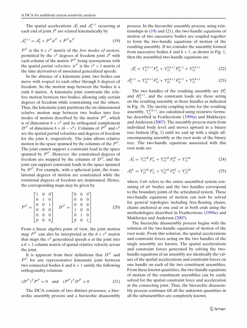
Consider two representative bodies, body k andbody k+1, of any articulated system as shown in Fig. 1.The joint between body k and body k+1 is referred toas Jk. Henceforth, any point on the body through whichthe interactions of the body with the environment canbe modeled would be referred to as a handle. Thehandles on a body can correspond to a joint location,a center of mass, or any desired reference point. Thetwo handles on body k corresponding to the locationsHk
1 and Hk2 are associated with joints Jk−1 and Jk,
respectively. Similarly, the two handles on body k+1corresponding to the locations Hk+1
1 and Hk+12 are asso-
ciated with joints Jk and Jk+1. Further, the accelerationof the handles Hk
1 and Hk2 and the constraint forces
acting on these points on body k will be denoted by thesuperscript k and subscripts 1 and 2, respectively.
In the most general form, the equations of motionfor body k using a spatial Newton–Euler formulationcan be expressed as
Mk0Ak
0 = Fk0 (9)
where
Mk0 =
[Ik
0 00 mk
], Ak
0 =[αk
0ak
0
], Fk
0 =[τ k
0f k0
](10)
In the above equations, the subscript 0 denotes thecenter of mass of the body, while superscript k indicatesthat the quantity is associated with representative bodyk. In (9) and (10), Mk
0 is the 6 × 6 spatial inertia matrixof k defined relative to a reference frame located at the

R.M. Mukherjee et al.
Fig. 1 Representative bodiesof a multibody system
body k body k+1
Joint Free-Motion Subspace P Jk
Assembly of
body k & body k+1
Relative motion embedded in inertia coupling terms and constraint forces at the boundary
b Assembly of bodies k and k+1a Representative bodies of an articulated system
F1ck
F2ck+1
F2ck F1c
k+1
F2ck+1
F1ck
H1k
H2k H1
k+1
H2k+1
H1k
H2k+1
point 0. It is composed of the 3 × 3 inertia matrix ofbody k about its mass center, the 3 × 3 diagonal massmatrix mk in which each diagonal element of the matrixis equal to the mass of body k, and 3 × 3 zero matrices0. The quantity Ak
0 is the 6 × 1 spatial acceleration as-sociated with the center of mass of body k in the inertialreference frame N. This matrix is composed of the 3 × 1angular acceleration vector αk of body k in N and thetranslational acceleration ak
0 of the body k mass centerin N. Similarly, Fk
0 is the resultant spatial loads matrixassociated with all loads (applied and constraint) actingon body k. This matrix is composed of the resultanttorque τ k
0 acting on body k with the resultant force f k0
acting on k with a line of action through the center ofmass of k. The total spatial load acting at the centerof mass consists of state-dependent active loads suchas actuators, loads from potential fields, and constraintforces arising from the joints. These constraint forcesdepend on the dynamics of the entire system, andhence, introduce coupling between the equations ofmotion of all bodies in the system. The active forces,on the other hand, are uncoupled and can be calculatedindependently on each body based on the state of thesystem. Thus, (9) can be written with Fk
0 expressedexplicitly in terms of the known active loads containedin Fk
a and the unknown constraint loads arising fromjoints Jk and Jk+1 as Fk
1c and Fk2c as
Mk0Ak
0 = Sk0k1Fk1c + Sk0k2Fk
2c + Fka (11)
Where
Sk0k1 =[
U rk0k1×0 U
]
6×6
(12)
And
Sk0k2 =[
U rk0k2×0 U
]
6×6
(13)
In the following description, a single body is assumedto have only two handles. However, this approach canbe easily extended to bodies with multiple handles. Thespatial equations of motion for body k can thus bewritten as
Ak1 =
[αk
ak1
]
(6×1)
= ζ k11 Fk
1c + ζ k12 Fk
2c + ζ k13 (14)
Ak2 =
[αk
ak2
]
(6×1)
= ζ k21 Fk
1c + ζ k22 Fk
2c + ζ k23 (15)
The above equation set is henceforth referred to asthe two-handle equations of motion of representativebody k. Ak
1 and Ak2 are then the spatial accelerations of
body k for handles Hk1 and Hk
2 , respectively. The termsζ k
ij (i, j = 1, 2) correspond to inertia coupling terms atthe joint locations on body k. Fk
1c and Fk2c are the
unknown spatial constraint loads acting on the body kat the handles Hk
1 and Hk2 , respectively, defined as
Fk1c =
[τ k
1cf k1c
]
(6×1)
and Fk2c =
[τ k
2cf k2c
]
(6×1)
(16)
with τ kic (3×1) and f k
ic (3×1) (i = 1, 2), representing theconstraint torques and constraint forces, respectively,being imposed at handles Hk
i . The active forces at thejoint are state-dependent and are treated as knownquantities. These are coupled together with the state-dependent inertia forces and expressed as ζij (i =1, 2; j = 3). Similarly, the two-handle equations ofmotion for body k+1 can be written in the form
Ak+11 = ζ k+1
11 Fk+11c + ζ k+1
12 Fk+12c + ζ k+1
13 (17)
Ak+12 = ζ k+1
21 Fk+12c + ζ k+1
22 Fk+12c + ζ k+1
23 (18)
A DCA for multibody system sensitivity analysis
The spatial accelerations Ak2 and Ak+1
1 occurring ateach end of joint Jk are related kinematically by
Ak+11 = Ak
2 + PJkuJk + PJk
uJk(19)
PJkis the 6 × νk matrix of the free modes of motion,
permitted by the νk degrees of freedom joint Jk witheach column of the matrix PJk
being synonymous withthe spatial partial velocities. uJk
is the νk × 1 matrix ofthe time derivatives of associated generalized speeds.
In the absence of a kinematic joint, two bodies canmove with respect to each other through 6 degrees offreedom. So the motion map between the bodies is arank 6 matrix. A kinematic joint constrains the rela-tive motion between two bodies, allowing only certaindegrees of freedom while constraining out the others.Thus, the kinematic joint partitions the six-dimensionalrelative motion map between two bodies into freemodes of motion described by the matrix PJk
, whichis of dimension 6 × νk and its orthogonal complementDJk
of dimension 6 × (6 − νk). Columns of PJkand νk
are the spatial partial velocities and degrees of freedomfor the joint k, respectively. The joint allows relativemotion in the space spanned by the columns of the PJk
.The joint cannot support a constraint load in the spacespanned by PJk
. However, the constrained degrees offreedom are mapped by the columns of DJk
, and thejoint can support constraint loads in the space spannedby DJk
. For example, with a spherical joint, the trans-lational degrees of motion are constrained while therotational degrees of freedom are maintained. Hence,the corresponding maps may be given by
PJk =
⎡
⎢⎢⎢⎢⎢⎢⎣
1 0 00 1 00 0 10 0 00 0 00 0 0
⎤
⎥⎥⎥⎥⎥⎥⎦DJk =
⎡
⎢⎢⎢⎢⎢⎢⎣
0 0 00 0 00 0 01 0 00 1 00 0 1
⎤
⎥⎥⎥⎥⎥⎥⎦(20)
From a linear algebra point of view, the joint motionmap PJk
can also be interpreted as the 6 × νk matrixthat maps the νk generalized speeds u at the joint intoa 6 × 1 column matrix of spatial relative velocity acrossthe joint.
It is apparent from their definitions that DJkand
PJkfor any representative kinematic joint between
two connected bodies k and k + 1 satisfy the followingorthogonality relations
(DJk)T PJk = 0 and (PJk
)T DJk = 0 (21)
The DCA consists of two distinct processes, a hier-archic assembly process and a hierarchic disassembly
process. In the hierarchic assembly process, using rela-tionships in (19) and (21), the two-handle equations ofmotion of two successive bodies are coupled togetherto form the two-handle equations of motion of theresulting assembly. If we consider the assembly formedfrom successive bodies k and k + 1, as shown in Fig. 1,then the assembled two-handle equations are
Ak1 = ϒk:k+1
11 Fk1c + ϒk:k+1
12 Fk+12c + ϒk:k+1
13 (22)
Ak+12 = ϒk:k+1
21 Fk1c + ϒk:k+1
22 Fk+12c + ϒk:k+1
23 (23)
The two handles of the resulting assembly are Hk1
and Hk+12 , and the constraint loads are those acting
on the resulting assembly at those handles as indicatedin Fig. 1b. The inertia coupling terms for the resultingassembly, ϒk:k+1
ij , are calculated using recursive formu-lae described in Featherstone (1999a) and Mukherjeeand Anderson (2007). The assembly process starts fromindividual body level and moves upward in a binarytree fashion (Fig. 1) until we end up with a single all-encompassing assembly as the root node of the binarytree. The two-handle equations associated with thisroot node are
A11 = ϒ1:nb
11 F11c + ϒ1:nb
12 Fnb2c + ϒ1:nb
13 (24)
Anb2 = ϒ1:nb
21 F11c + ϒ1:nb
22 Fnb2c + ϒ1:nb
23 (25)
where 1:nb refers to the entire assembled system con-sisting of nb bodies and the two handles correspondto the boundary joints of the articulated system. Thesetwo-handle equations of motion can now be solvedfor general topologies including free-floating chains,chains anchored at one end or at both ends using themethodologies described in Featherstone (1999a) andMukherjee and Anderson (2007).
The hierarchic disassembly process begins with thesolution of the two-handle equations of motion of theroot node. From this solution, the spatial accelerationsand constraint forces acting on the two handles of thesingle assembly are known. The spatial accelerationsand constraint forces generated by solving the two-handle equations of an assembly are identically the val-ues of the spatial accelerations and constraint forces onone handle on each of the two constituent assemblies.From these known quantities, the two-handle equationsof motion of the constituent assemblies can be easilysolved for the spatial constraint force and accelerationat the connecting joint. Thus, the hierarchic disassem-bly process continues till all the unknown quantities inall the subassemblies are completely known.

R.M. Mukherjee et al.
3.2 Sensitivity formulation
From the previous section, the two-handle equations ofmotion of a body k can be written as follows
Ak1 = ζ k
11Fk1 + ζ k
12Fk2 + ζ k
13 (26)
Ak2 = ζ k
21Fk1 + ζ k
22Fk2 + ζ k
23 (27)
In the above equations, the matrices ζ k11 and ζ k
22 are sym-metric positive definite (SPD), and the matrices ζ k
12 andζ k
21 are transposes of each other. The matrices ζ k13 and
ζ k23 include the terms that are state-dependent (for, e.g.,
the active forces) and can be calculated independentlyon each body. Similar expressions for body k + 1 can bewritten as
Ak+11 = ζ k+1
11 Fk+11 + ζ k+1
12 Fk+12 + ζ k+1
13 (28)
Ak+12 = ζ k+1
21 Fk+11 + ζ k+1
22 Fk+12 + ζ k+1
23 (29)
Let pj represent any design variable with respect towhich the sensitivity of the dynamic system’s objectivefunction J is to be calculated. For a dynamic system,pj may be a mass or inertia value, geometric constantsuch as length, radius, or active force among others.Differentiating (26) and (27) with respect to pj, thefollowing equations are derived.
dAk1
dpj= dζ k
11
dpjFk
1 + ζ k11
dFk1
dpj
+ dζ k12
dpjFk
2 + ζ k12
dFk2
dpj+ dζ k
13
dpj(30)
dAk2
dpj= dζ k
21
dpjFk
1 + ζ k21
dFk1
dpj+
+ dζ k22
dpjFk
2 + ζ k22
dFk2
dpj+ dζ k
23
dpj(31)
With
d(Mk0)
−1
dpj= −(Mk
0)−1 dMk
0
dpj(Mk
0)−1 (32)
In the above equations, the terms dζ kij /dpj can be
easily obtained from d(Mk0)/dpj and dSk0ki/dpj lo-
cally on each body, as there is no coupling in theseterms from other bodies in the system. These terms arezero when pj is a design variable that is not local to thebody k. The other terms, viz. dFk
i /dpj and dAki /dpj
(i = 1 : 2), cannot be calculated locally on each body, asthese depend on the coupling between different bodiesin the system. Further, by solving the equations ofmotion (26) and (27) at any instant, the terms Fk
i (i =1 : 2) are generated. Thus, having solved the equationsof motion at any instant, (30) and (31) reduce to thefollowing form with the only unknowns at each bodybeing the terms dFk
i /dpj and dAki /dpj (i = 1 : 2).
dAk1
dpj= �k
11dFk
1
dpj+ �k
12dFk
2
dpj+ �k
13 (33)
dAk2
dpj= �k
21dFk
1
dpj+ �k
22dFk
2
dpj+ �k
23 (34)
where
�k13 = dζ k
11
dpjFk
1 + dζ k12
dpjFk
2 + dζ k13
dpj(35)
and
�k23 = dζ k
21
dpjFk
1 + dζ k22
dpjFk
2 + dζ k23
dpj(36)
with
�kij = dζ k
ij
dpjfor i , j = 1:2 (37)
The corresponding equations for body k + 1 can beexpressed as
dAk+11
dpj= �k+1
11
dFk+11
dpj+ �k+1
12
dFk+12
dpj+ �k+1
13 (38)
dAk+12
dpj= �k+1
21
dFk+11
dpj+ �k+1
22
dFk+12
dpj+ �k+1
23 (39)
Thus, (26) and (27) and (33) and (34) are in thesame analytical form, albeit with different quantitiesin the equations. Further, (33) and (34) are obtainedin the desired form only if (26) and (27) have alreadybeen solved. Thus, the basic procedure is: (1) solve thedynamics equations of motion to generate the valuesof the constraint forces at each body; (2) substitutethe values for the constraint forces in (30) and (31) togenerate (33) and (34). These are now the sensitivityequations of each body that need to be solved.

A DCA for multibody system sensitivity analysis
4 Two-handle generalized inertia
The relative acceleration between two joint locationson successive bodies k and k + 1 can be expressed interms of the free modes of motion matrix PJk
and thegeneralized speeds at the joint uJk
as
Ak+11 − Ak+1
2 = PJkuJk + PJk
uJk(40)
Differentiating the above equation with respect toparameter pj,
dAk+11
dpj− dAk
2
dpj= PJk duJk
dpj
+ dPJk
dpjuJk + PJk duJk
dpj+ dPJk
dpjuJk
︸ ︷︷ ︸Locally Generated
(41)
⇒ dAk+11
dpj− dAk
2
dpj= PJk duJk
dpj+ � (42)
where
� = dPJk
dpjuJk + dPJk
dpjuJk + PJk duJk
dpj(43)
In the above equations, locally generated terms de-pend only on the state sensitivities and can be treatedas known quantities. Further, from Newton’s third law,the loads acting through joint Jk as seen by bodies kand k + 1 are equal and opposite.
Fk2 = −Fk+1
1 ⇒ dFk2
dpj= −dFk+1
1
dpj(44)
Substituting the expressions for dAk2/dpj and
dAk+11 /dpj from (34), (35), (36), (37), (38), and (39)
into (41), respectively, and using the relationships (21),the following expressions can be derived:
dAk+11
dpj− dAk
2
dpj= �k+1
11
dFk+11
dpj+ �k+1
12
dFk+12
dpj+ �k+1
13
−�k21
dFk1
dpj− �k
22dFk
2
dpj− �k
23 (45)
⇒[�k+1
11 +�k22
] dFk+11
dpj=
[�k
21dFk
1
dpj−�k+1
12
dFk+12
dpj
+ �k23−�k+1
13
+PJk dudpj
+�
](46)
Pre-multiplying (46) by (DJk)T and calling on the or-
thogonality condition between DJkand PJk
,
(DJk)T
[�k+1
11 + �k22
] dFk+11
dpj
= (DJk)T
[�k
21dFk
1
dpj+�k
23
− �k+113 − �k+1
12
dFk+12
dpj+ �
]
+ (DJk)T PJk
︸ ︷︷ ︸0
dudpj
(47)
From the definition of the orthogonal complement ofjoint motion subspace, the constraint force Fk+1
1 canbe expressed in terms of the measure numbers of theconstraint torques and constraint forces as
Fk+11 = DJk
Fk+11 (48)
⇒ dFk+11
dpj= dDJk
dpjFk+1
1 + DJk dFk+11
dpj(49)
where the constraint force and constraint moment mea-sure numbers f1c
k+1and ˜τ1c
k+1, respectively, are repre-sented as
Fk+11 =
[˜τ1c
k+1
f1ck+1
](50)
Substituting this into (47), an expression fordFk+1
1 /dpj can be derived as below:
DJk T [�k+1
11 + �k22
](dDJk
dpjFk+1
1 + DJk dFk+11
dpj
)
= DJk T[�k
21dFk
1
dpj+�k
23−�k+113 −�k+1
12
dFk+12
dpj+�
]
(51)
⇒ dFk+11
dpj= X
[�k
21dFk
1
dpj+ �k
23 − �k+112
dFk+12
dpj
−�k+113
]− dDJk
dpjFk+1
1 (52)
where X = DJk([DJk ]T [�k
22 + �k+111 ]DJk
)−1[DJk]T
(53)

R.M. Mukherjee et al.
Substituting this expression for dFk+11 /dpj and
dFk2 /dpj into (33), (34), (35), (36), (37), (38), and (39),
the following are obtained:
dAk1
dpj= �k:k+1
11
dFk1
dpj+ �k:k+1
12
dFk+12
dpj+ �k:k+1
13 (54)
dAk+12
dpj= �k:k+1
21
dFk1
dpj+ �k:k+1
22
dFk+12
dpj+ �k:k+1
23 (55)
In substituting the expression for the derivative of theconstraint load at the common joint, the equations ofthe derivatives of the spatial accelerations of the twobodies are coupled together to form the correspondingequations of the resulting assembly. In the resultingassembly, the two joints that connect the assembly toits parent and child bodies (or assemblies) are Jk
1 andJk+1
2 . The �k:k+1ij are the inertia coupling terms of the
assembly of bodies k and k + 1 given by
�k:k+111 = [
�k11 − �k
12X�k21
](56)
�k:k+112 =
[�k
12X�k+112
](57)
�k:k+113 =
[�k
13 − �k12X�k+1
13
](58)
�k:k+121 =
[�k+1
21 X�k21
](59)
�k:k+122 =
[�k+1
22 − �k+121 X�k+1
12
](60)
�k:k+123 =
[�k+1
23 + �k+121 X�k+1
23
](61)
5 Hierarchic assembly–disassembly
In the previous section, a set of recursive formulaewere derived that may be used to couple together thesensitivity equations of two adjacent bodies to formthe corresponding equations of the resulting assem-bly. In the associated manipulations, the two bodiesare coupled together to form an assembly by express-ing the derivative of the intermediate (common) jointconstraint load with respect to the design variable interms of the corresponding derivatives of the constraintforces at the other two handles. This process can nowbe repeated for all bodies in the system where theequations of two successive bodies or assemblies arecoupled together using the recursive formulae to obtainthe corresponding equations of the resulting assembly.This process works hierarchically exploiting the samestructure as that of a binary tree.
This process begins at the level of individual bodiesof the system. Adjacent bodies of the system are hierar-chically assembled to construct a binary tree as shown
in Fig. 2. Individual bodies that make up the systemform the leaf nodes of the binary tree. The sensitivityequations of motion of a pair of bodies are coupledtogether using the recursive set of formulae (56), (57),(58), (59), (60), and (61) to form the correspondingequations of the resulting assembly. The resulting as-sembly now corresponds to a node of the next level inthe binary tree. Working along the binary tree in thishierarchic assembly process, only a single assembly isleft at the root node of the binary tree. The root nodecorresponds to the two-handle representation of theentire articulated system modeled as a single assem-bly. The sensitivity equations of this root node can beexpressed as
dA11
dpj= �1:nb
11dF1
1
dpj+ �1:nb
12dFnb
2
dpj+ �1:nb
13 (62)
dAnb2
dpj= �1:nb
21dF1
1
dpj+ �1:nb
22dFnb
2
dpj+ �1:nb
23 (63)
Here, the superscript 1:nb is used to denote the wholesystem being represented as a single entity as the rootnode of the binary tree. In this case, the handles 1and 2 of this entity are the boundary joints of thearticulated system. Similarly, the derivatives of the spa-tial constraint loads are those of the spatial constraintloads arising from the interaction of the system with itsboundaries. The above equations represent two sets ofequations in terms of four sets of unknowns, i.e., thederivatives of the spatial accelerations at the boundaryjoints dA1
1/dpj and dAnb2 /dpj and the derivatives of
the corresponding constraint loads and dF11 /dpj and
dFnb2 /dpj . Consider the three following scenarios that
may arise for a system.
1 2 3 4 5 6
1+2 3+4 5+6
1+2+3+4 5+6
1+2+3+4+5+6
Hierarchic D
isassembly
Single all inclusive assembly : Root Node
Actual bodies of the system : Leaf Nodes
Hie
rarc
hic
Ass
embl
y
Intermediateassembly level nodes
Fig. 2 The hierarchic assembly and disassembly process usingbinary tree structure

A DCA for multibody system sensitivity analysis
5.1 Free floating
This case corresponds to a system that is free floating,i.e., there are no kinematic joints connecting the systemto the inertial frame. In the absence of any kinematicjoints at either boundary, there are no constraint forcesthat can act on the system at the boundaries. In thiscase, in (62) and (63), the constraint loads terms are allzero, and hence, their derivatives are always zero. Fromthis, the derivatives of the spatial accelerations can beeasily solved as
dA11
dpj= �1:nb
13 anddAnb
2
dpj= �1:nb
23 (64)
5.2 Anchored at one end by kinematic joint
In this case, the system is connected to the inertialframe by a kinematic joint at one end while the otherend is free floating. For such a system, there is noconstraint load acting at the free end, and in (62) and(63), the term dFnb
2 /dpj = 0, and hence, its deriva-tive is also always zero. However, at the other end, thesystem will experience a constraint load because of thepresence of the kinematic joint and its derivative needsto be accounted for. The equations in this case reduceto
dA11
dpj= �1:nb
11dF1
1
dpj+ �1:nb
13 (65)
dAnb2
dpj= �1:nb
21dF1
1
dpj+ �1:nb
23 (66)
From the definition of the kinematic joint and itsjoint motion map, there exist the following kinematicrelations:
dA11
dpj= P1 du1
dpj+ dP1
dpju1 + d(P1u1)
dpj︸ ︷︷ ︸Locally generated
(67)
⇒ dA11
dpjP1 du1
dpj+ � (68)
where
� = dP1
dpju1 + d(P1u1)
dpj(69)
Further, from the definition of the orthogonal com-plement of the joint motion map, the constraint load atthe handle can be expressed as
F11 = D1F1
1 ⇒ dF11
dpj= dD1
dpjF1
1 + D1 dF11
dpj(70)
Substituting (67), (68), (69), and (70) into (65) and(66), the following are derived.
P1 du1
dpj+ � = �1:nb
11 [dD1
dpjF1
1 + D1 dF11
dpj] + �1:nb
13 (71)
⇒ P1 du1
dpj= �1:nb
11 [dD1
dpjF1
1 + D1 dF11
dpj] + �1:nb
13 −� (72)
Using the orthogonality relation between P1 and D1,the derivative of the generalized speed at the joint aswell as that of the constraint load can be solved from(72) as
D1TP1
︸ ︷︷ ︸0
du1
dpj= D1T
�1:nb11 D1 dF1
1
dpj
+ D1T[�1:nb
11dD1
dpjF1
1 + �1:nb13 − �
](73)
⇒ dF11
dpj= −D1
[(D1)T�1:nb
11 D1]−1
(D1)T
×[�1:nb
11dD1
dpjF1
1 + �1:nb13 − �
](74)
⇒ du1
dpj= P1
[(P1)T(�1:nb
11 )−1 P1]−1
(P1)T
×[�1:nb
11dD1
dpjF1
1 + �1:nb13 − �
](75)
Substituting (74) and (75) into (65) and (66), thederivatives of the boundary spatial accelerations, i.e.,dA1
1/dpj and dA11/dpj , can be easily calculated.
5.3 Anchored at both ends by kinematic joints
In this case, the system is connected to the inertialframe by a kinematic joint at both ends, and the sys-tem reduces to a kinematically closed-loop topology.For such a system, there are constraint loads acting atboth ends due to the kinematic joints. In this case, thesensitivity equations for the system remain
dA11
dpj= �1:nb
11dF1
1
dpj+ �1:nb
12dFnb
2
dpj+ �1:nb
13 (76)
dAnb2
dpj= �1:nb
21dF1
1
dpj+ �1:nb
22dFnb
2
dpj+ �1:nb
23 (77)

R.M. Mukherjee et al.
Similar to the previous situation, the following kine-matic relations exist between the boundary joints andtheir joint motion maps.
dA11
dpj= P1 du1
dpj+ dP1
dpju1 + d(P1u1)
dpj︸ ︷︷ ︸Locally generated
and
dAnb2
dpj= Pnb dunb
dpj+ dPnb
dpjunb + d(Pnb unb )
dpj︸ ︷︷ ︸Locally generated
(78)
⇒ dA11
dpj= P1 du1
dpj+ �1
and
dAnb2
dpj= Pnb dunb
dpj+ �2 (79)
where
�1 = dP1
dpju1 + d(P1u1)
dpj
and
�2 = dPnb
dpjunb + d(Pnb unb )
dpj(80)
Further, from the definition of the orthogonal com-plement of the joint motion map, the constraint load atthe handle can be expressed as
F11 = D1F1
1 ⇒ dF11
dpj= dD1
dpjF1
1 + D1 dF11
dpj(81)
Fnb2 = Dnb Fnb
2 ⇒ dFnb2
dpj= dDnb
dpjFnb
2 + Dnb dFnb2
dpj
(82)
Substituting (79) into (76) and (77) and absorbingthe terms �i into the �1:nb
i3 term (i = 1 : 2), one obtains
P1 du1
dpj= �1:nb
11dF1
1
dpj+ �1:nb
12dFnb
2
dpj+ �1:nb
13 (83)
Pnb dunb
dpj= �1:nb
21dF1
1
dpj+ �1:nb
22dFnb
2
dpj+ �1:nb
23 (84)
Multiplying the above equations by (D1)T and(Dnb )T , respectively, and calling on the orthogonalityrelation, the following are obtained.
0︷ ︸︸ ︷(D1)T P1 du
dpj
1
= (D1)T[�1:nb
11dF1
1
dpj
+ �1:nb12
dFnb2
dpj+ �1:nb
13
]= 0 (85)
(Dnb )T Pnb︸ ︷︷ ︸
0
dunb
dpj= (Dnb )T [�1:nb
21dF1
1
dpj
+ �1:nb22
dFnb2
dpj+ �1:nb
23 ] = 0 (86)
Substituting the expressions for the derivatives of theconstraint loads from (81) and (82) into (85) and (86),one obtains
(D1)T�1:nb11 D1 dF1
1
dpj+ (D1)T�1:nb
12 Dnb dFnb2
dpj
+(Dnb )T[�1:nb
11dD1
dpjF1
1 + �1:nb12
dDnb
dpjFnb
2
+�1:nb13
]= 0 (87)
(Dnb )T�1:nb21 D1 dF1
1
dpj+ (Dnb )T�1:nb
22 Dnb dFnb2
dpj
+(Dnb )T[�1:nb
21dD1
dpjF1
1 + �1:nb22
dDnb
dpjFnb
2
+�1:nb23
]= 0 (88)
In these equations, (D1)T�1:nb11 D1 and (Dnb )T�1:nb
22Dnb are SPD matrices, and there is no problem associ-ated with their inversion. For notational convenience,the above equations can be represented compactly inmatrix form as[χ11 χ12
χ21 χ22
] [dF1
1/dpj
dFnb2 /dpj
]= −
[χ13
χ23
](89)
where the corresponding χij can be derived from theabove equation. The matrix in (89) is also SPD withχ12 = χT
21. The above set of equations can now be easilysolved. Having solved the above equations for the val-ues of dF1
1/dpj and dFnb2 /dpj , the corresponding ex-
pression for dF11 /dpj and dFnb
2 /dpj can be obtainedfrom (81) and (82). At this point, the derivatives ofboth constraint loads on the boundary joints are known.Consequently, (76) and (77) of the root node can besolved to obtain the derivatives of the spatial accel-erations dA1
1/dpj and dA11/dpj at the corresponding
joints.

A DCA for multibody system sensitivity analysis
Thus, in all three cases, the derivatives of the spatialaccelerations and the constraint loads at the boundaryjoints can be calculated. This initiates the hierarchic dis-assembly process. The derivatives of the spatial accel-erations and the constraint loads generated by solvingthe sensitivity equations of an assembly are identicallythe values of the derivatives of the spatial accelera-tions and the constraint loads on one handle on eachof the two constituent assemblies. From these knownquantities, the sensitivity equations of the constituentassemblies can be solved to obtain the derivatives of thespatial accelerations and that of the constraint loads atthe connecting joint. For example, for a representativeassembly made from body k and body k+1, the sensi-tivity equations are given by (54) and (55). On solvingthese equations, the quantities dAk
1/dpj , dAk+12 /dpj ,
dFk1 /dpj , and dFk+1
2 /dpj are generated. These quan-tities are then substituted into the sensitivity equationsof the constituent sub-assemblies body k and body k+1.Thus, knowing the values of dAk
1/dpj and dFk1 /dpj ,
(33) and (34) can be solved, while from dAk+12 /dpj
and dFk+12 /dpj , (38) and (39) can also be solved. This
process is repeated in a hierarchic disassembly of the bi-nary tree where the known derivatives of the boundaryconditions are used to solve the sensitivity equations ofthe immediate sub-assemblies, until derivatives of thespatial acceleration and constraint forces on all bodiesin the system are calculated.
6 Discussion
In the previous section, the method for calculatingthe sensitivities of multibody dynamics systems in thethree general topologies is described. These topologiesinclude free-floating kinematic chains, kinematic chainsanchored at one end, and topologies with kinemati-cally closed loops. The sensitivity analysis is based onthe forward dynamics algorithms (Featherstone 1999a;Mukherjee and Anderson 2007) and gains from the in-herent capabilities of these methods. The calculation ofthe sensitivities is simplified by exploiting the topologyof the system and the fundamental idea of the joint freemodes of motion map and its orthogonal complement.The local derivatives used in the algorithm are tem-porally invariant and exact. These are generated onceduring a preprocessing step and introduced into the al-gorithm as an input. This algorithm works in six sweepsof the system, traversing the system topology like abinary tree. The first four sweeps are associated withformulating and solving the equations of motion for theforward dynamics problem. The next two sweeps areassociated with the sensitivity analysis and correspond
to the hierarchic assembly and the hierarchic disassem-bly processes, respectively. These last two sweeps mayadditionally be performed concurrently with the finaltwo sweeps of the forward dynamics formulation if theconcurrent formulation is preferred. The concurrentformulation is an implementation detail with a minormanipulation of the equations and is not described inthis paper. The concurrent formulation would reducethe number of sweeps of the topology from six to fourwhere the sensitivity analysis could be performed inlock-step with the forward dynamics problem.
Modeling systems in kinematically closed-looptopologies has traditionally been an interesting prob-lem in multibody dynamics because of the presenceof explicit loop closure constraints. Along with thedynamics equations of motion of an equivalent un-constrained system, traditional methods maintain theconstraints through an extra set of algebraic equa-tions, which are used to either (1) reduce out excessivedegrees of freedom producing a minimum dimensionsystem of equations, or (2) augment the equations ofmotion producing a larger dimension system of equa-tions involving redundant state variables. This givesrise to two primary problems: (1) the saddle pointproblem originating from constraint equations becom-ing numerically dependent and (2) the accumulationof integration errors leading to significant drift in con-straint satisfaction. Because most methods for sensitiv-ity analysis of multibody dynamics systems are based onthe forward dynamics method, the sensitivity analysis ofthese systems suffers from the same drawbacks as theforward dynamics methods in handling kinematicallyclosed loops.
However, in the method described in this paper, theloop closure constraint is modeled using a different ap-proach. Instead of using explicit constraint equations,the constraints are implicitly imposed by describingthe topology of the system through the relative co-ordinates and the use of a set of redundant general-ized coordinates to enforce the loop closure constraint.The redundant set of generalized coordinates maintainsthe definition of the kinematic joint that converts anunconstrained system into a constrained system in aloop configuration. The presence of an extra kinematicjoint introduces an additional orthogonality relationbetween the map of the free modes of motion, the joint,and its orthogonal complement. This allows for the loopclosure constraint to be implicitly imposed. Further,the use of a redundant set of generalized coordinatesalways maintains the correct dimensionality of the sys-tem equations, making this algorithm free from rankdeficiency issues as all matrices to be inverted are SPD.This ensures that the algorithm can robustly handle

R.M. Mukherjee et al.
what would normally be considered singular configura-tions. The manner in which this method avoids singular-ities appears similar, in some regards, to that of Eulerparameters. With Euler parameters, one deals with aredundant four-member set of generalized coordinates(parameters) for the global and nonsingular descriptionof general spatial rotation. The constraints betweenthese four coordinates are implicitly enforced. If theconstraints were explicitly used to reduce out the extrageneralized coordinate (parameter), the representationagain may become singular. In the same manner, thisalgorithm enforces the constraints implicitly, thereby,avoiding singularities.
The problem of constraint violation is not completelyeliminated in this algorithm because the constraintsare imposed at the acceleration level. However, per-formance of this algorithm on sample test cases asdiscussed in Mukherjee and Anderson (2007) indicatesthat the method is able to maintain the constraint vi-olation growth at a minimum rate and perform com-parable to (or better than) methods with velocity levelconstraint imposition. The imposition of the constraintsat the velocity and position level within the frameworkof this algorithm continues to be a research endeavor.
7 Computational complexity and parallel aspects
In the previous sections, the sensitivity analysis for anygiven multibody system is explained using six sweepstraversing the topology of the system. However, asexplained before, the implementation can use foursweeps where the sensitivity information is generatedconcurrently with the solution of the forward dynam-ics problem. While the concurrent implementation canfurther improve the computational efficiency, for easeof understanding, the discussion is limited to the six-sweep process.
The generation of the derivative primitives is de-pendent on the system under consideration and thedesign parameters. Consequently, the derivative prim-itives can be calculated numerically, analytically, orempirically. The generation of the derivative primitivesis a preprocessing step and needs to be done once(potentially for an entire family of simulations). Hence,it is not considered in the computational complexityof this algorithm. Once the derivative primitives havebeen developed, the algorithm proceeds in the sameway as the forward dynamics problem. The forwarddynamics problem is based on the divide-and-conquerscheme and has been detailed in Featherstone (1999a)and Mukherjee and Anderson (2007). The sensitivityanalysis method described in this paper cannot function
independent of the forward dynamics problem, as thesensitivity analysis requires the determination of accel-erations and the constraint forces before calculating thesensitivities. Thus, a large number of the entities usedin the sensitivity analysis are already developed for theforward dynamics problem. Consequently, the first twosweeps of the method are analogous to the first twosweeps of the forward dynamics problem.
The additional cost incurred in the sensitivity analy-sis is associated with the coupling of the sensitivityequations of successive bodies using the hierarchicassembly process and then the subsequent solutionof these equations using the hierarchic disassemblyprocess. In serial implementation, the hierarchic as-sembly and disassembly processes work recursively andsolve the sensitivity problem in linear or O(n) complex-ity, where n is the number of degrees of freedom of thesystem. The cost associated with the recursive solutionin serial implementation has been studied in detail inHsu and Anderson (2002) and is similarly applicable tothis algorithm.
For parallel implementation, this algorithm isprocessor and time-optimal, solving the sensitivityproblem in O(log(n)) complexity in the presence of nprocessors, where n now is the number of bodies in thesystem. In the presence of n processors, each body ofthe system is mapped onto a different processor wherethe sensitivity problem for that body is formulated. Themapping of the bodies onto the processors is developedin a binary tree representation as shown in Fig. 2. Thehierarchic assembly–disassembly process then worksvia two traversals of the binary tree. These traversalswork exactly in the same fashion as for the forward dy-namics problem (Featherstone 1999b) and are achievedin O(log(n)) complexity. This highly parallel aspectof the algorithm arises from the nature of the sen-sitivity equations for individual bodies or assemblies.As discussed previously, the equations are cast in thetwo-handle form where the problem is posed in termsof the interactions of the body or an assembly withits boundaries by expressing the internal unknownsas functions of boundary unknowns. This allows theassembly–disassembly process to proceed in an order-independent, concurrent form, facilitating high parallelefficiency.
In the presence of a modest number of processors,the system is divided into assemblies equal to thenumber of processors available. Within each processor,the equations of the corresponding assembly can beformulated in linear complexity to express the problemin terms of the boundary unknowns of the assembly,similar to the serial implementation. The calculationof the boundary unknowns proceeds using the binary

A DCA for multibody system sensitivity analysis
Fig. 3 Four-bar: closed-loop mechanism
tree representation of the system, where the leaf nodesnow correspond to the assemblies instead of the phys-ical bodies. This is achieved in logarithmic complexity.On completing this, the boundary unknowns of everyassembly in the system are known. Using these values,the sensitivity equations of the bodies in each assemblycan be solved in linear complexity using the recursiveprocess as in the serial implementation. This linearcomplexity process is carried out concurrently for all as-semblies. The number of bodies in the different assem-blies and the actual computational gains would dependon different parameters such as load balancing, multi-processor architecture, the method for inter-processorcommunications, and costs, among implementation-dependent aspects.
Fig. 4 Sensitivity comparison with reference solution fordu1/dLa
Fig. 5 Double pendulum: serial chain
8 Numerical examples
The sensitivity values generated using the algorithmdescribed above are verified by simulating multibodysystem test cases previously presented in literature.Results from two test cases are presented here. Thesetest cases were chosen to demonstrate the ability of thealgorithm to accurately generate sensitivity informationfor serial chain systems as well as systems with a kine-matically closed loop.
The first test case is a kinematically closed-loop sys-tem consisting of three rigid links A, B, and C con-
Fig. 6 Sensitivity comparison with reference solution fordq1/dLa

R.M. Mukherjee et al.
nected by revolute joints to form a four-bar mechanismas shown in Fig. 3. The system is released from restwith the initial configuration of q1 = 30, q2 = 44.4775,and q4 = 45.5225 degrees, respectively, under the effectof gravity. The length and mass of the links in thesystem are La = 1 m, Lb = Lc = 2 m, ma = 10, mb =mc = 20 kg, and gravity = 9.81. The sensitivity of u1
with respect to La (du1/dLa) is calculated for a 10-ssimulation and shown in Fig. 4.
The next system considered is a double pendu-lum moving under the effect of gravity as shown inFig. 5. The system parameters are La = Lb = 1 m,Ma = Mb = 1 m, q1 = q2 = π/30 radians, and gravity =9.81 m/s2. The mechanism is released from rest. Forthis system, the sensitivity of q1 with respect to La
(dq1/dLa) is calculated, and the results are shown inFig. 6.
In both cases, the results obtained are comparedagainst established results obtained from the directdifferential method as described in Anderson and Hsu(2004). The results obtained using the new algorithmare in excellent agreement with the reference solutions.The results clearly demonstrate the ability of the al-gorithm to provide sensitivity values accurate up tointegration tolerance. For the system in closed-loopconfiguration, the method does not suffer from exces-sive constraint violations.
9 Conclusions
In this paper, a new efficient method is presented forsensitivity analysis of multibody systems. The methoduses a direct differentiation approach and implements itin a divide-and-conquer scheme. The method maps thetopology of the system to a binary tree and generatesthe sensitivity information using several traversals ofthis binary tree. The computational complexity of thisalgorithm is expected to be linear and logarithmic inserial and parallel implementations, respectively. Themethod works in tandem with the forward dynam-ics problem. Consequently, there is no excessive datastorage and no backward integration in this scheme.Thus, the method does not suffer from numerical issuesassociated with perturbations in design variables. Themethod is robust and does not suffer from numericaldependency issues associated with singular configura-tions. The low computational cost of the algorithm,its simplicity in implementation, applicability for serialand closed-loop systems, insensitivity to numerical anddata storage issues, and accuracy of results make thisalgorithm a useful tool in sensitivity analysis for multi-body dynamics systems.
Acknowledgements This work was funded by the NSF NIRTGrant Number 0303902. The authors thank the funding agencyfor their support.
References
Anderson KS, Hsu YH (2001) Low operational order analyticsensitivity analysis for tree-type multibody dynamic systems.J Guidance Control Dyn 24(6):1133–1143
Anderson KS, Hsu YH (2004) ‘Order-(n+m)’ direct differen-tiation determination of design sensitivity for constrainedmultibody dynamic systems. Struct Multidisc Optim 26(3–4):171–182
Bestle D, Eberhard P (1992) Analysing and optimizing multibodysystems. Struct Machines 20:67–92
Bestle D, Seybold J (1992) Sensitivity analysis of constrained op-timization in dynamic systems. Archive Appl Mech 62:181–190
Bischof CH (1996) On the automatic differentiation of computerprograms and an application to multibody systems. In: Pro-ceedings of the IUTAM symposium on optimization of me-chanical systems, pp 41–48
Chang CO, Nikravesh PE (1985) Optimal design of mechani-cal systems with constaint violation stabilization method. JMech Trans Autom Des 107:493–498
Dias J, Pereira M (1997) Sensitivity analysis of rigidflexible multi-body systems. Multibody Syst Dyn 1(3):303–322
Eberhard P (1996) Analysis and optimization of complex multi-body systems using advanced sensitivity methods. MathMech 76:40–43
Etman L (1997) Optimization of multibody systems using ap-proximation concepts. PhD thesis, Technische UniversiteitEindhoven, The Netherlands
Featherstone R (1999a) A divide-and-conquer articulated bodyalgorithm for parallel O(log(n)) calculation of rigid body dy-namics. Part 1: Basic algorithm. Int J Robot Res 18(9):867–875
Featherstone R (1999b) A divide-and-conquer articulated bodyalgorithm for parallel O(log(n)) calculation of rigid bodydynamics. Part 2: Trees, loops, and accuracy. Int J Robot Res18(9):876–892
Haug E, Ehle PH (1982) Second-order design sensitivity analysisof mechanical system dynamics. Int J Numer Methods Eng18:1699–1717
Haug E, Wehage RA, Mani NK (1984) Design sensitivity analy-sis of large-scaled constrained dynamic mechanicsl systems.Trans ASME 106:156–162
Hsu YH, Anderson KS (2002) Recursive sensitivity analysis forconstrained multi-rigid-body dynamic systems design opti-mization. Struct Multidisc Optim 24(4):312–324
Jain A, Rodrigues G (2000) Sensitivity analysis of multibodysystems using spatial operators. In: Proceedings of the inter-national conference on method and models in automationand robotics (MMAR 2000), Miedzyzdroje, Poland
Kim SS, VanderPloeg MJ (1986) Generalized and efficientmethod for dynamic analysis of mechanical systems usingvelocity transforms. J Mech Trans Autom Des 108(2):176–182
Mukherjee R, Anderson KS (2007) An orthogonal complementbased divide-and-conquer algorithm for constrained multi-body systems. Nonlinear Dyn 48(1-2):199–215
Nikravesh PE (1990) Systematic reduction of multibody equa-tions to a minimal set. Int J Non Linear Mech 25(2-3):143–151

A DCA for multibody system sensitivity analysis
Pagalday J, Aranburu I, Avello A, Jalon JD (1995)Multibody dynamics optimization by direct differentia-tion methods using object oriented programming. In:Proceedings of the IUTAM symposium on optimiza-tion of mechanical systems, Stuttgart, Germany, pp 213–220
Serban R, Haug EJ (1998) Kinematic and kinetics deriva-tives for multibody system analyses. Mech Struct Machines26(2):145–173
Tak T (1990) A recursive approach to design sensitivity analysisof multibody systems using direct differentiation. PhD thesis,University of Iowa, Iowa City