A New Economic Framework: A DSGE Modelwith Cryptocurrency∗

Stylianos Asimakopoulos† Marco Lorusso‡

Francesco Ravazzolo§

July 17, 2020

Abstract

We develop and estimate a DSGE model to evaluate the economicrepercussions of cryptocurrency. We assume that cryptocurrency offersan alternative currency option to government currency, with endogenoussupply and demand. We uncover a substitution effect between thereal balances of government currency and cryptocurrency in response totechnology, preferences and monetary policy shocks. We also observe acountercyclical reaction of real balances of cryptocurrency to these shocks.Cryptocurrency productivity shocks have negative effects on output, inflationand cryptocurrency exchange rate. Finally, output and inflation responsesare stronger when cryptocurrency is introduced in the utility function in anon-separable way.

Keywords: DSGE Model, Government Currency, Cryptocurrency,Bayesian Estimation.JEL classification: E40, E41, E51, E52.

∗We would like to thank Paolo Gelain, John Sessions, Harald Uhlig and the conferenceparticipants at the 12th Conference on Computational and Financial Econometrics, the27th Annual Symposium of the Society for Nonlinear Dynamics and Econometrics, the25th International Conference Computing in Economics and Finance, the 15th DynareConference and the University of Sydney Macroeconomic Reading Group Workshop.†University of Bath, Department of Economics.‡Newcastle University Business School, Department of Economics.§Corresponding author: francesco.ravazzolo@unibz.it. Free University of Bozen-

Bolzano and CAMP, BI Norwegian Business School.

1 Introduction

Cryptocurrency has recently gained considerable interest from investors,

central banks and governments worldwide. There are numerous reasons

for this intensified attention. For example, Japan and South Korea have

recognised Bitcoin as a legal method of payment (Bloomberg, 2017a;

Cointelegraph, 2017). Some central banks are exploring the possibility of

using cryptocurrency (Bloomberg, 2017c). Moreover, a large number of

companies and banks have created the Enterprise Ethereum Alliance1 in

order to customise Ethereum for industry players (Forbes, 2017). Finally,

the Chicago Mercantile Exchange (CME) started the Bitcoin futures on 18th

December 2017 (Chicago Mercantile Exchange, 2017).2

In this paper, we develop and estimate a Dynamic Stochastic General

Equilibrium (DSGE) model in order to evaluate the economic repercussions

of cryptocurrency. Our model includes the demand and supply of

cryptocurrency by extending and reformulating standard DSGE models with

money (see, among others, Nelson, 2002, Christiano et al., 2005, Ireland,

2004) with the new sector of the economy related to cryptocurrency. Our

analysis allows us to compare the responses of real money balances for

government currency and cryptocurrency to several demand and supply

shocks driving the economy. Moreover, we are able to evaluate the response

of the main macroeconomic fundamentals to productivity shocks for the

production of cryptocurrency.

In 2017 the value of cryptocurrencies experienced exponential growth and

their market capitalization substantially increased. However, the volatility

of cryptocurrencies has been very significant with regular daily swings of up

to 30%. Figure 1 provides evidence of these characteristics by showing the

1Source: https://entethalliance.org/members/.2Nasdaq and Tokyo Financial Exchange followed in 2018 (Bloomberg, 2017b; Tokyo

Financial Exchange, 2017).

2

Coinbase Index (CBI).3

By 2017, Bitcoin, the first decentralised cryptocurrency that was

created in 2008 and documented in Nakamoto (2008), had grown to a

maximum of approximately 2,700% price return and, in the same year,

some cryptocurrencies had achieved far higher growth than Bitcoin. Some

economists, famous investors, and finance professionals warned that the

rapidly increasing prices of cryptocurrencies could cause the “bubble” to

burst. In fact, in early 2018, a large sell-off of cryptocurrencies occurred.

From January to February 2018, the price of Bitcoin fell by 65%, and by

the end of the first quarter of 2018, the entire cryptocurrency market fell by

54%, with losses in the market topping USD 500 billion. The decline of the

cryptocurrency market was larger than the bursting of the Dot-com bubble

in 2002. In November 2018, the total market capitalisation for Bitcoin fell

below USD 100 billion for the first time since October 2017, and the Bitcoin

price fell below 5,000 USD. More recently, the Bitcoin price has partially

recovered and, in summer 2019, it traded at levels higher than 10,000 USD.

As we can observe from Figure 1, such dynamics have been shared by all

types of cryptocurrencies.

Cryptocurrency is the private sector counterpart of government-issued

currency (Nakamoto, 2008; Ethereum, 2014; Ripple, 2012) and is issued

in divisible units that can be easily transferred in a transaction between

two parties. Digital currencies are intrinsically useless electronic tokens

that travel through a network of computers. Advances in computer science

have allowed for the creation of a decentralised system for transferring these

electronic tokens from one person or firm to another. The key innovation

of the cryptocurrency system is the creation of a payment system across a

network of computers that does not require a trusted third party to update

3The CBI tracks the combined financial performance of all of the digital assets listedfor trading in the US region by Coinbase. The components of the CBI are weighted bymarket capitalization, defined as price multiplied by supply.

3

balances and keep track of the ownership of the virtual units. The technology

behind the system is called Blockchain.4

The characteristics of cryptocurrency are as follows. The first

characteristic relates to the fact that cryptocurrency is not based on a

central authority that holds private information. On the contrary, it

relies on public information, such as computation, from a large number of

individual distributed computers and servers connected to each other via

the network and not by a recognised authority. Secondly, the issue of new

currency and operations are validated by the network via complex pre-defined

mathematical operations, an algorithm defined as proof of work. This kind

of network approves pre-defined, encrypted and immutable operations, so

history cannot be changed and manipulated. The last characteristic refers to

the ease of payment and management. Cryptocurrency is, by definition,

computer-based and when linked to a portfolio the only requirement for

transferring value or paying bills is an internet connection.

Most previous studies have analysed cryptocurrency empirically. For

example, Hencic and Gourieroux (2014) applied a non-causal autoregressive

model to detect the presence of bubbles in the Bitcoin/USD exchange

rate. Sapuric and Kokkinaki (2014) measured the volatility of the Bitcoin

exchange rate against six major currencies. More recently, Catania et al.

(2018) analysed and predicted cryptocurrency volatility, whereas Catania

et al. (2019) predicted the full distribution of cryptocurrency. Both Bianchi

(2018) and Giudici and Pagnottoni (2019) have investigated the structural

relationships between cryptocurrency and other macroeconomic and financial

time-series.

However, there have only been a few theoretical studies that have

modelled cryptocurrency. In this regard, Boehme et al. (2015) introduced

the economics, technology and governance of Bitcoin, whereas Fernandez-

4Cryptocurrency is just one of the many applications of Blockchain.

4

Villaverde and Sanches (2019) developed a model of competition among

privately-issued fiduciary currencies. Garratt and Wallace (2018) and

Schilling and Uhlig (2019) focused on the exchange rate of Bitcoin and its

theoretical determinants. Brunnermeier and Niepelt (2019) derived a model

of money and liquidity in order to identify the sources of seignorage rents and

liquidity bubbles in the context of cryptocurrency. As we will explain in the

next section, most of these studies have assumed partial equilibrium models

and did not examine the economic repercussions from the introduction of

cryptocurrency to the overall economy and its different sectors.

We try to fill this gap and we develop a Dynamic Stochastic General

Equilibrium (DSGE) where cryptocurrency is considered as the alternative

to government currency. In our model, we assume that the utility function

is non-separable across consumption and real balances of government

currency and cryptocurrency in household preferences. Moreover, we include

two separate demand shocks to government currency and cryptocurrency,

respectively.

We estimate our model with Bayesian techniques using US and

cryptomarkets monthly data for the period 2013:M6-2019:M3. Specifically

we construct two new series to proxy the quantity of cryptocurrency and

technological development, respectively. To the best of our knowledge,

our work is the first attempt to provide a general equilibrium model with

cryptocurrency and to estimate its parameters with Bayesian techniques.

Our estimated results confirm the assumption of non-separability between

consumption and real balances of government currency and cryptocurrency.

Comparing this data-driven finding with the related literature that allows

assets or wealth to enter household preferences in an additive separable

way (see, among others, Iacoviello, 2015 and Michaillat and Saez, 2019), we

contribute to the ongoing debate concerning the nature of cryptocurrency

by suggesting that cryptocurrency should be treated similarly to government

currency. In this regard, our empirical results are in line with Gans and

5

Halaburda (2019) that have defined cryptocurrency as a private digital

currency.5

Our empirical analysis indicates that the reaction of the economy to

shocks in preferences, technology and monetary policy are in line with the

findings of previous literature (see, for example, Ireland, 2004 and Andres

et al., 2009). In addition, the reaction of real balances of cryptocurrency is

countercyclical to output in response to these shocks. Moreover, in response

to technology and monetary policy shocks, we find a strong substitution effect

between the real balances of government currency and the real balances of

cryptocurrency.

Our results show that the economy responds differently to shocks in

the demand for government currency and cryptocurrency. In particular,

government currency demand shocks have larger effects on output, inflation

and the nominal interest rate. We also find that cryptocurrency productivity

shocks imply a fall in the nominal exchange rate between government

currency and cryptocurrency. The increase in the productivity of

cryptocurrency leads to lower real balances of government currency due to

the substitution effect. In turn, both output and inflation fall, whereas the

inflation rate increases. However, the magnitude of these effects is much

lower than in the case of preference, technology and monetary policy shocks.

We are able to quantify the contributions of each shock in our model

through a variance decomposition analysis. Our findings indicate that

technology, preferences and monetary policy have the highest contribution

in terms of variations in the key endogenous variables of our model. We

also find that specific productivity shocks play an important role in the

variation of real balances of cryptocurrency and nominal exchange rate

5An alternative strand of literature defines cryptocurrency as a cryptoasset or utilitytokens, see Boreiko et al. (2019) for a review of the various definitions, becausecryptocurrency is no yet full “money-like” due to its current limitations and has moreuses than a form of money payment, including investment purposes (see https://www.

bankofengland.co.uk/knowledgebank/what-are-cryptocurrencies).

6

between government currency and cryptocurrency.

Our analysis allows us to test for the role of the non-separability

assumption between consumption and real balances of cryptocurrency. Our

findings show that the functional form of the utility function matters in terms

of the responses of several macroeconomic aggregates to cryptocurrency

productivity shocks. In particular, a gain in cryptocurrency productivity

induces stronger decreases in output and inflation in the case of non-separable

utility function between consumption and real balances of cryptocurrency.

Finally, we assess the role of monetary policy in the presence of shocks

to cryptocurrency productivity. Our sensitivity analysis indicates that the

larger the response of the monetary policy rule to a change in government

currency growth is, the stronger the decline in output.

Our study also provides two policy recommendations. Firstly, we show

that an increase in cryptocurrency productivity has a negative effect on

output. Therefore, the monetary authority could adjust its policy rate in

response to changes in the real balances of cryptocurrency and include a

weight for cryptocurrency growth in its policy reaction function. Secondly,

we provide evidence that the response of the nominal interest rate to changes

in government currency growth needs to be gradual in order for the central

bank to mitigate the fall in output.

The remainder of this paper is organised as follows. Section 2 reviews

the relevant literature. Section 3 outlines the new DSGE model on

which our study is based. In Section 4, we present the data used for

the analysis and our Bayesian estimates. Section 5 presents the impulse

response functions based on our estimated model. In Section 6, we focus

on the variance decomposition analysis. In Section 7, we assess the

choice of utility function by distinguishing the cases of non-separable and

separable household preferences between consumption and real balances

of cryptocurrency. Section 8 provides a sensitivity analysis on different

assumptions concerning the monetary policy rule. The concluding remarks

7

are found in Section 9.

2 Literature review

Our paper refers to two different streams of literature. On the one

hand, we contribute to studies that have developed theoretical models to

analyse and describe cryptocurrency dynamics. However, these studies have

focused mainly on partial equilibrium models. In our work, we develop a

general equilibrium framework introducing cryptocurrency as an alternative

to government currency. On the other hand, our study also contributes to

the DSGE literature that has analysed the role of government currency in

the economy.

Regarding the first strand of literature and the theoretical models,

Boehme et al. (2015) presented the design principles and properties of

Bitcoin’s platform for a non-technical audience. They reviewed past, present,

and future uses of Bitcoin, identifying risks and regulatory issues as Bitcoin

interacts with the conventional financial system and the real economy.

Furthermore, Fernandez-Villaverde and Sanches (2019) built a model of

competition among privately-issued fiduciary currencies.6 They found that

the lack of control over the total supply of money in circulation has critical

implications for the stability of prices across the economy. In other words,

the economy ends up in a state of hyperinflation. These authors also showed

that in the short and medium terms, the value of digital currencies goes up

and down unpredictably as a result of self-fulfilling prophecies.

Another theoretical model analysing the exchange rate between fiat

currency and Bitcoin was developed by Athey et al. (2016). In particular,

they argued that the Bitcoin exchange rate can be fully determined by two

market fundamentals: the steady-state transaction volume of Bitcoin when

6More specifically, Fernandez-Villaverde and Sanches (2019) extended the Lagos andWright (2005) model by including entrepreneurs who can issue their own currencies tomaximise profits following a predetermined algorithm (as in Bitcoin).

8

used for payments, and the evolution of beliefs about the likelihood that

the technology will survive. Garratt and Wallace (2018) also studied the

behaviour of the Bitcoin-to-Dollar exchange rate. They used the model

introduced by Samuelson (1958) with identical two-period lived overlapping

generations with one good per date. After exploring the problems of pinning

down money prices in the one-money model, these authors expanded their

analysis to include a competing outside fiat money (Bitcoin), and they also

discussed other aspects of competing cryptocurrencies.

More recently, Sockin and Xiong (2018) developed a model in which the

cryptocurrency has two main roles: (i) to facilitate transactions of certain

goods among agents; (ii) as the fee to compensate coin miners for providing

clearing services for the decentralised goods transactions on the platform. As

a consequence of the first role of cryptocurrency, households face difficulties

in making such transactions as a result of severe search frictions. In turn,

such rigidity induced by the cryptocurrency price leads to either no or two

equilibria.

Schilling and Uhlig (2019) used a model in the spirit of Samuelson

(1958), assuming that there are two types of money: Bitcoins and fiat

money such as dollars. Both monies can be used for transactions. These

authors found a “fundamental condition”, which is a version of the exchange-

rate indeterminacy result in Kareken and Wallace (1981), showing that

the Bitcoin price in dollar terms follows a martingale, adjusted for the

pricing kernel. Schilling and Uhlig (2019) also found that there is a

“speculative condition”, in which the dollar price for the Bitcoin is expected

to rise, and some agents start hoarding Bitcoin in anticipation of the price

increase. Finally, Brunnermeier and Niepelt (2019) developed a dynamic and

stochastic model with heterogeneous households, firms, and banks, as well as

the government sector. They demonstrated that a swap from public money

to private money does not imply a credit crunch nor undermine financial

stability.

9

However, most of the aforementioned theoretical studies have utilised

partial equilibrium models. In our work, we develop a general equilibrium

set-up. Many DSGE models have analysed the role of government currency

in the economy. For example, Nelson (2002) presented empirical evidence for

the US and the UK that real money base growth matters for real economic

activity. In particular, they have shown that the presence of the long-term

nominal rate in the money demand function increases the effect of nominal

money stock changes on real aggregate demand when prices are sticky.

In addition, Christiano et al. (2005) developed a model embodying

nominal and real rigidities that accounts for the observed inertia in inflation

and persistence in output. They included money among the variables of

interest and found that the interest rate and the money growth rate move

persistently in opposite directions after a monetary policy shock.

A small monetary business cycle model which contains three equations

summarising the optimising behaviour of the households and firms that

populate the economy was developed by Ireland (2004). This author found

that, if changes in the real stock of money have a direct impact on the

dynamics of output and inflation, then that impact must come simultaneously

through both the IS and the Phillips curve. In the same spirit, Andres et al.

(2009) have analysed the role of money in a general equilibrium framework

focusing on the US and the EU. Their findings uncovered the forward-looking

character of money demand.

Therefore, our work can be seen as an extension of these studies that

redefines the standard DSGE model with money by including a new sector

of the economy related to cryptocurrency, thereby generating endogenous

supply and demand in a general equilibrium framework. In the next

section, we present our structural model of the monetary business cycle with

cryptocurrency in detail.

10

3 Model

3.1 Households

The representative household of the economy maximises the following

expected stream of utility:

max{Ct,Ht,Bt,Mg

t ,Mct }E

∞∑t=0

βtAt

[u

(Ct,

Mgt

Pt

Egt

,χt

Mct

Pt

Ect

)− ηHt

](1)

where 0 < β < 1 and η > 0. The budget constraint each period is given by:

M gt−1 + χt−1M

ct−1 + Tt +Bt−1 +WtHt +Dt = PtCt +

Bt

Rt

+M gt + χtM

ct (2)

The variableMgt

Ptrepresents the real balance for government currency,

whereasMct

Ptdenotes the real balance for the cryptocurrency. Moreover, χt

indicates the nominal exchange rate between the government currency and

the cryptocurrency.

Equation (1) shows that consumption and real balances of government

currency and cryptocurrency are non-separable. This non-separability makes

the marginal utility of consumption a function of the amount of real balances

of government currency and cryptocurrency optimally demanded by the

households. Our approach implies that cryptocurrency is a private digital

currency that is the alternative with respect to government currency.7

Moreover, since cryptocurrency can be seen as an alternative currency that

does not pay any interest, in equation (2) we assume that the representative

household purchases cryptocurrency at t−1 in terms of government currency,

M ct−1 =

Mgt−1

χt−1, and holds cryptocurrency at time t as M c

t =Mgt

χt.8

7In particular, the fact that cryptocurrency enters into the utility function of therepresentative household implies that the government accepts it as a form of payment.Therefore, cryptocurrency can be used for any economic transaction and can be expressedin terms of government currency through the nominal exchange rate.

8In this regard, our modelling differs from standard open economy DSGE models withmultiple currencies (see, among others, Bodenstein et al., 2011). In these models theexchange rate is used to convert the interest rate received by the representative household

11

In equations (1) and (2), Ct and Ht denote household consumption and

labour supply during the period t. The shocks At, Egt and Ec

t follow the

autoregressive processes:

ln (At) = ρa ln (At−1) + εat (3)

ln (Egt ) = ρeg ln

(Egt−1

)+ εegt (4)

ln (Ect ) = ρec ln

(Ect−1

)+ εect (5)

where 0 < ρa, ρeg, ρec < 1 and the zero-mean, serially uncorrelated

innovations εat , εegt and εect are normally distributed with standard deviations

σa, σeg and σec. As we are going to show below, in equilibrium, shock

At translates into disturbances to the model’s IS curve, whereas Egt and

Ect indicate disturbances to government money and cryptocurrency demand

curves.

In the budget constraint, household sources of funds include Tt, a lump-

sum nominal transfer received from the monetary authority at the beginning

of period t, and Bt−1, the value of nominal bonds maturing during period t.

The household’s sources of funds also include labour income, WtHt, where

Wt denotes the nominal wage, and nominal dividend payments, Dt, received

from the intermediate goods-producing firms. The household’s uses of funds

consist of consumption, Ct, of finished goods, purchased at the nominal price,

Pt, newly-issued bonds of value BtRt

, where Rt denotes the gross nominal

interest rate.

It is convenient going forward to denote household real balances of

government currency and cryptocurrency by mgt =

Mgt

Ptand mc

t =Mct

Pt,

respectively. Moreover, we denote the gross inflation during period t with

πt = PtPt−1

.

into holding foreign bonds. On the contrary, in our model the exchange rate allows fortwo currencies (i.e. government currency and cryptocurrency) that are used in the sameeconomy to be converted.

12

3.2 Entrepreneurs

We assume that there is a continuum of entrepreneurs indexed by n, where

n ∈ [0, 1], producing cryptocurrency. Each representative entrepreneur

operates under a perfect competition. Following Sockin and Xiong (2018),

we introduce a cost of producing cryptocurrency given by: κ−φtQct , where Qc

t

is the amount of tokens that the entrepreneur is producing. In addition:

φt = ξt + νt (6)

is the entrepreneur’s productivity, which depends on the productivity of

the other entrepreneurs via the common component, ξt, as well as on the

specific programming skills of the entrepreneur, νt. We assume that ξt and

νt represent the common and specific productivity shocks to producing costs

following the autoregressive processes:

ln (ξt) = ρξ ln (ξt−1) + εξt (7)

ln (νt) = ρν ln (νt−1) + ενt (8)

where 0 < ρξ, ρν < 1, and the zero-mean, serially uncorrelated innovations,

εξt and ενt , are normally distributed with standard deviations σξ and

συ. Entrepreneurs also gain a fraction (1− ρ) ∈ (0, 1) from selling the

cryptocurrency to households at price Ptχt

. Thus, entrepreneurs maximise

their profits with respect to Qct :

Πt = max{Qct}

((1− ρ)

Ptχt− κ−φt

)Qct (9)

3.3 Production Goods Firms

We assume a continuum of monopolistically competitive firms indexed

by i ∈ [0, 1] producing differentiated varieties of intermediate production

goods, and a single final production good firm combining the variety of

intermediate production goods under perfect competition. During each

13

period t = 0, 1, 2, ..., the representative final goods-producing firm uses Yt (i)

units of each intermediate good purchased at the nominal price, Pt (i), to

manufacture Yt (i) units of the final goods according to the constant-returns

to-scale technology described by:

Yt =

1∫0

Yt (i)(θ−1)θ di

θ

(θ−1)

(10)

where θ > 1. The final goods-producing firm maximises its profits by

choosing:

Yt (i) =

(Pt (i)

Pt

)−θYt (11)

which reveals that θ measures the constant price elasticity of demand for

each intermediate good. Competition drives the final goods-producing firm’s

profits to zero in equilibrium, determining Pt as:

Pt =

1∫0

(Pt (i))1−θ di

1

1−θ

(12)

During each period t = 0, 1, 2, ..., the representative intermediate goods-

producing firm hires Ht (i) units of labour from the representative household

to manufacture Yt (i) units of intermediate good i according to the linear

technology:

Yt (i) = ZtHt (i) (13)

where the aggregate productivity shock, Zt, follows the autoregressive

process:

ln (Zt) = ρz ln (Zt−1) + εzt (14)

where 0 < ρz < 1, and the zero-mean, serially uncorrelated innovation, εzt , is

normally distributed with standard deviation σz. In equilibrium, this supply-

side disturbance acts as a shock to the Phillips curve. Since the intermediate

goods substitute imperfectly for one another in producing the final goods,

14

the representative intermediate goods-producing firm sells its output in a

monopolistically competitive market: the firm acts as a price-setter, but must

satisfy the representative final goods-producing firm’s demand at its chosen

price. Similar to Rotemberg (1982), the intermediate goods-producing firm

faces a quadratic cost of adjusting its nominal price, measured in terms of

the final goods and given by:

φ

2

[Pt (i)

πPt−1 (i)− 1

]2

Yt (15)

with φ > 0 and π measuring the gross steady-state inflation rate. This cost

of price adjustment makes the intermediate goods-producing firm’s problem

dynamic: it chooses Pt (i) for all t = 0, 1, 2, ... to maximise its total market

value. At the end of each period, the firm distributes its profits in the form

of a nominal dividend payment, Dt (i), to the representative household.

3.4 Monetary Policy

We assume that the central bank sets the nominal interest rate following a

modified version of the Taylor (1993) rule given by:

ln

(Rt

R

)= ρr ln

(Rt−1

R

)+ (1− ρr) ρy ln

(YtY

)+

(1− ρr) ρπ ln(πtπ

)+ (1− ρr) ρµg ln

(µgtµg

)+ εrt (16)

where:

µgt =

Mgt

PtMgt−1

Pt−1

(17)

In equation (16), ρr, ρy, ρπ and ρµg

are non-negative parameters, and the

zero-mean, serially uncorrelated policy shock, εrt , is normally distributed with

the standard deviation σr. The monetary authority adjusts the short-term

nominal interest rate in response to deviations of output and inflation from

their steady-state levels as well as government currency growth as shown in

equation (17). Andres et al. (2009) have argued that an interest-rate rule

15

that depends on the change in real balances of government currency may

be motivated as part of an optimal reaction function when money growth

variability appears in the central bank’s loss function. As an alternative

explanation, the response to money growth can be justified by money’s

usefulness in forecasting inflation.

3.5 Equilibrium

The symmetric equilibrium of the model can be log-linearised to obtain the

following set of equations9:

yt = yt+1 − ω1 (rt − πt+1) + ω2

[(mg

t − egt )−

(mgt+1 − e

gt+1

)]+ (18)

ω3

[(χt + mc

t − ect)−(χt+1 + mc

t+1 − ect+1

)]+ ω1 (at − at+1)

mgt = γ1yt − γ2rt + γ3e

gt − γ4χt − γ4m

ct + γ4e

ct (19)

mct = γ5yt − γ6rt + γ7e

ct − γ8χt − γ8m

gt + γ8e

gt (20)

πt =( πR

)πt+1 + ψ

(1ω1

)yt −

(ω2

ω1

)(mg

t − egt )

−(ω3

ω1

)(χt + mc

t − ect)− zt

(21)

χt = −%φt (22)

φt =

(ξ

φ

)ξt +

(1− ξ

φ

)νt (23)

rt = ρrrt−1 + (1− ρr) ρyyt + (1− ρr) ρππt + (1− ρr) ρµg µgt + εrt (24)

Equation (18) represents a log-linearised version of the Euler equation that

links the household’s marginal rate of intertemporal substitution to the real

interest rate. When ω2 and ω3 are different from zero, the household’s

utility function is non-separable across consumption and real balances of

government currency and cryptocurrency. Since utility is non-separable, real

balances of government currency and cryptocurrency affect the marginal rate

9The small letters with a hat, xt, denote the deviation of a given variable, Xt, fromits steady-state value. The full derivation of the model together with the steady statesolutions are shown in Appendix A.

16

of intertemporal substitution. Hence, additional terms involving mgt and mc

t

also appear in the IS curve.

Equation (19) takes the form of a money demand relationship for

government currency, with income elasticity (γ1), interest semi-elasticity (γ2),

elasticity of mgt with respect to government currency demand shocks (γ3), and

cross-elasticity with cryptocurrency (γ4).10 Moreover, equation (20) reveals

the form of a money demand relationship for cryptocurrency, with income

elasticity (γ5), interest semi-elasticity (γ6), elasticity of mct with respect to

cryptocurrency demand shocks (γ7), and cross-elasticity with government

currency (γ8).11

Equation (21) is a forward-looking Phillips curve that also allows real

balances of government currency (mgt ) and cryptocurrency (mc

t) to enter

into the specification when ω2 and ω3 are non-zero. The non-separability

in preferences across consumption and real balances of government currency

and cryptocurrency implies a direct influence of the former variable on

marginal cost and inflation; hence, real balances of government currency

and cryptocurrency also appear in the Phillips curve.

Equations (18) and (21) also reveal that, wherever the real balances of

government currency (mgt ) and cryptocurrency (mc

t) appear in the IS and

Phillips curve relationships, they are followed immediately by the money

demand disturbances, egt and ect .

Equation (22) is the log-linearised first order condition derived from

the profit maximisation problem of entrepreneurs that shows a negative

relationship between the entrepreneurs’ productivity and the exchange

10In equation (19), we note that an increase in the demand for cryptocurrency decreasesthe real balances of government currency. In Section 4.4, we will show that the estimatedvalue of the cross elasticity of government currency demand and cryptocurrency demandis high.

11Equation (20) indicates that the real balances of cryptocurrency decrease when thedemand of government currency rises. In Section 4.4, our estimated results will showthat the value of γ8 is above unity, indicating a strong substitution effect betweencryptocurrency and government currency.

17

rate between government currency and cryptocurrency. This expression

reflects the well-established feature of cryptocurrency that is based on a

cryptographic proof-of-work system. Such system relies on solving complex

mathematical operations and generating new coins with this validation.

The process is known as mining. Nakamoto (2008) proposed a largest

pool of central processing unit (CPU). However, since 2011, a graphical

processing unit (GPU) has revolutionised the computational power and its

introduction has stimulated the diffusion of Bitcoin. In our model, this

mechanism can be interpreted as a positive productivity shock for the mining

of cryptocurrency, reducing the exchange rate value between government

currency and cryptocurrency.

Equation (23) is the log-linearised expression for the entrepreneurs’

productivity that depends on the common productivity in the cryptocurrency

sector as well as on the specific productivity of the entrepreneur. Equation

(24) shows the log-linearised relation for the monetary policy rule, indicating

that the interest rate adjusts to output, inflation and government currency

growth.

The cryptocurrency market is in equilibrium if the quantity of

cryptocurrency supplied by entrepreneurs is equal to the demand of

cryptocurrency by households. The goods market clearing condition implies

that the output produced by production goods firms is equal to households’

consumption. The model is closed by adding the log-linearised versions of

the AR(1) processes for the preferences shock to consumption, the demand

shocks for government currency and cryptocurrency, the common and specific

productivity shocks of cryptocurrency as well as the aggregate technology

shock.

18

4 Estimating the Model

In this section, we estimate the model described in Section 3 using Bayesian

techniques. In what follows, we initially describe the data used in order to

estimate the model (Section 4.1). Successively, we present the parameters

of the model (Section 4.2) and their identification (Section 4.3). Finally, we

describe the estimation results (Section 4.4).

4.1 Data

The main challenge in estimating our model is the relatively short sample

for the macroeconomic series related to the market of cryptocurrency due to

its recent development. Accordingly, in order to have a sufficient number

of observations for our estimated model, we decided to use US data at

monthly frequency. Foroni and Marcellino (2014) have dealt with DSGE

models estimated with mixed frequency data, including monthly data. Our

sample period corresponds to 2013:M6-2019:M3. We use seven data series in

the estimation because there are seven shocks in the theoretical model (see

Table 1).12

The seven data series include the industrial production index, the natural

log of real private consumption, the natural log of real money stock, the real

Bitcoin price, the real cumulative initial coin offering (ICO), the real Nvidia

volume weighted average price and the effective federal funds rate. All the

real variables are deflated by the consumer price index (CPI). Real private

consumption and real M2 money stock are expressed in per capita terms,

divided by working-age population.

Focusing on monetary variables, we follow Ireland (2004) by considering

money stock M2 as an indicator that includes a broader set of financial

assets held principally by households. The real Bitcoin price is obtained

12The data sources and the construction of all observed variables are reported inAppendix B.

19

from the monthly average of daily data, assuming that the daily price is the

average between opening and closing prices. We consider the Bitcoin price

to be representative of the cryptocurrency price. Our choice is related to

the longer sample period that is available for the Bitcoin price compared to

the CBI. Our assumption is plausible since, for the same sample period, the

correlation between the CBI and the Bitcoin price corresponds to 99%.

The ICO or initial currency offering is a type of funding which uses

cryptocurrency. In an ICO, a quantity of cryptocurrency is sold in the form

of tokens to speculator investors, in exchange for legal tender or another

cryptocurrency. The tokens sold are promoted as future functional units

of currency if the ICO’s funding goal is met and the project is launched.

The Nvidia volume weighted average price is obtained as a monthly average

from daily data. The Nvidia Corporation is the most important American

technology company that designs graphics processing units (GPUs) for the

gaming and professional markets, as well as systems on chip units (SoCs) for

the mobile computing and automotive market.

4.2 Model Parameters

We decided to split the parameters of the model into two groups. The first

group of parameters is fixed and consistent with data at a monthly frequency.

In line with Ireland (2004), we assume ω1 equal to one, implying the same

level of risk aversion as a utility function that is logarithmic in consumption.

The parameter ψ is fixed equal to 0.1 following King and Watson (1996),

Ireland (2000) and Ireland (2004). Such a value implies that the fraction

of the discounted present value and future discrepancies between the target

price and the actual price of production goods is equal to 10%. The steady-

state values for the nominal interest rate and inflation are computed from the

monthly data of the effective federal funds rate and natural log changes in

CPI. For our sample period they are equal to 0.70% and 0.13%, respectively.

20

The second group of parameters is estimated with the Bayesian technique

(Tables 2 and 3). To the best of our knowledge, our study is the first attempt

to estimate a DSGE model that includes cryptocurrency. Hence, this is one

of our main contributions and we rely on our judgement and the findings

of previous DSGE models that consider government currency (e.g., Ireland,

2000, Ireland, 2004 and Andres et al., 2009).

Table 2 shows the prior distributions for the endogenous parameters of

our model. For the parameter indicating the output elasticity with respect

to real balances of government currency (ω2), we assume that its prior mean

is in line with the range of estimates by Ireland (2004). On the other hand,

we assume that the prior mean of the elasticity of output with respect to real

balances of cryptocurrency (ω3) is one fourth lower than that of government

currency.

In order to set up the priors for the income elasticity of government

currency demand (γ1), the interest semi-elasticity of government currency

demand (γ2) and the elasticity of real balances of government currency with

respect to government currency demand shocks (γ3), we follow the estimated

results of Ireland (2004) for the US economy. Moreover, we assume a prior

mean value for γ4 such that changes in the demand for cryptocurrency can

affect the real balances of government currency.

Focusing on the parameters that characterise the demand relationship

for cryptocurrency, we assume that γ6 has a higher prior mean value than

γ5. Moreover, we assume that the real balances of cryptocurrency are

strongly affected by exogenous changes in cryptocurrency demand, which

corresponds to a large prior mean for γ7. Moreover, following Gans and

Halaburda (2019), we believe that cryptocurrency is a valuable alternative

to government currency and assume a high prior mean value for γ8.

In line with Athey et al. (2016) and Garratt and Wallace (2018),

we acknowledge that the exchange rate between government currency

and cryptocurrency is an important determinant of the cryptocurrency

21

productivity and, in turn, we assume a high prior mean value for %.

Turning to the parameter measuring the relative importance of common

productivity with respect to specific productivity in the production of

cryptocurrency ( ξφ), we are agnostic about its prior and, in turn, we assume

that it covers a reasonable range of values.

Regarding the parameters of the monetary policy rule, the prior for the

degree of interest rate smoothing (ρr), the reaction coefficient of output (ρy),

the interest-rate response to inflation (ρπ) and government currency growth

(ρµg) are all in line with the estimates by Andres et al. (2009).

Table 3 reports the priors of the parameters related to the exogenous

processes driving the economy. We set the persistence parameters of all

autoregressive exogenous processes to be Beta distributed. We assume that

the technology shock is more persistent than consumption preference and

government currency demand shocks. We also assume that the prior for

the persistence of the cryptocurrency demand shock has a relatively low

value. For both productivity shocks to cryptocurrency, we assume that

their prior means and standard deviations correspond to 0.60 and 0.05,

respectively. Finally, we use Inverse Gamma distributions for standard errors

of all exogenous shocks with means equal to 0.01 and infinite degrees of

freedom which correspond to rather loose priors.

4.3 Parameter Identification

We estimated our model using a sample of 5,000,000 draws and we dropped

the first 1,250,000.13 Our acceptation rate corresponds to 37%. In order

to test the stability of the sample, we used the Brooks and Gelman (1998)

diagnostics test, which compares within and between moments of multiple

chains. Moreover, we performed other diagnostic tests for our estimates, such

as the Monte Carlo Markov Chain (MCMC) univariate diagnostics and the

13In order to perform our estimation analysis, we used Dynare(http://www.dynare.org/).

22

multivariate convergence diagnostics.14

As it is well known, the lack of identification in the parameter values

is a potentially serious problem for the quantitative implications of DSGE

models (see, for example Canova and Sala, 2009). Accordingly, we compared

the prior and posterior distributions of the model parameters. For most

of the parameters we found that prior probability density functions are

wide, and posterior distributions are different from the priors.15 Moreover,

we performed the test proposed by Iskrev (2010).16 This test checks the

identification strength and sensitivity component of the parameters using a

rank condition based on the Fischer information matrix and the moment

information matrix normalised by either the parameter at the prior mean

or by the standard deviation at the prior mean. Our results show that the

derivative of the vector of predicted autocovariogram of observables with

respect to the vector of estimated parameters has full rank when we evaluate

it at the posterior mean estimate. This implies that all the parameters are

identifiable in the neighbourhood of our estimates.

4.4 Estimated Results

Tables 2 and 3 show the posterior means for the endogenous and exogenous

parameters with their 90% confidence intervals.

We start by focusing on the estimated parameters of the IS curve. From

Table 2, we note that the estimated posteriors of ω2 and ω3 are different from

zero. This result indicates that the utility function is non-separable between

consumption and real balances of government currency and cryptocurrency.

Interestingly, the estimated values ω2 and ω3 imply that the output response

to changes in real balances of government currency is more than six times

14The plots for MCMC univariate and multivariate convergence diagnostics are shownin Appendix C.

15We report the plots for prior and posterior density functions of all parameters inAppendix C.

16The plots showing the results for this test are reported in Appendix D.

23

higher compared to variations in real balances of cryptocurrency. As we will

see in the next section, this result has important consequences for the effects

of cryptocurrency productivity shocks on the economy.

Turning to the parameters of the money demand equation for government

currency, our estimated values of γ1, γ2 and γ3 are in line with the ranges

of estimates provided by Ireland (2004), implying that the demand shock

(egt ) has the highest influence on the movements in the real balances of

government currency. Moreover, the estimated posterior of γ4 is well

identified and indicates an important degree of substitution between the

demand of government currency and cryptocurrency.

Now we focus on the estimated parameters included in the money demand

equation for cryptocurrency. From Table 2, it is possible to note that the

posterior mean of γ6 is much higher than γ5, implying that real balances

of cryptocurrency respond more to changes in nominal interest rate than to

variations in output. As will be shown in Section (5), this result has an

important effect in terms of the response of cryptocurrency demand to the

preference shock. Moreover, we find that the posterior means of γ7 and γ8 are

above unity. These results have two main implications. Firstly, they suggest

that the demand shock (ect) plays a substantial role in terms of variation in

the real balances of cryptocurrency. Secondly, our estimates indicate a strong

elasticity of substitution between cryptocurrency and government currency.

This result will be discussed further in the next section. In particular, we

are going to show that the change in government currency demand greatly

affects the demand for cryptocurrency.

Focusing on the parameters related to the production of cryptocurrency,

the estimated posterior of % is well identified and has a value slightly below

unity. Our result confirms the studies by Garratt and Wallace (2018) and

Athey et al. (2016) who found that the exchange rate between government

currency and cryptocurrency is an important determinant of cryptocurrency

production. Moreover, the estimated value of ξφ

suggests that common

24

productivity has a stronger impact than the specific productivity in terms of

cryptocurrency production. This implies that common productivity shocks

have larger effects on the economy than specific productivity shocks.

Turning to the estimates of the monetary policy reaction function, we

observe that in our sample period there is significant interest-rate smoothing.

In addition, the nominal interest rate appears to react more strongly to

variations in the inflation rate than to output changes. Interestingly, our

estimated parameter for the interest-response to government currency growth

(ρµg) has a higher value than in Andres et al. (2009). This result suggests

that the central bank relies on the government currency growth to set up its

policy rate.

Table 3 shows the posterior estimates for the exogenous processes. In

general, the posteriors of these parameters are well identified. We note

that technology and preference shocks are more persistent than government

currency and cryptocurrency demand shocks. Moreover, we find that

the specific productivity shock to cryptocurrency production is slightly

more persistent than the common productivity shock to cryptocurrency

production. Finally, our posterior estimates show that shocks to specific

cryptocurrency productivity, cryptocurrency and government currency

demand are much more volatile than the remaining shocks.

5 Impulse Response Functions

In this section, we show the results of impulse response functions (IRFs)

for the estimated model and consider some of the exogenous shocks driving

the economy. Firstly, we focus on the “traditional” shocks to preferences,

technology and monetary policy. Secondly, we analyse the shocks to

the demand of households for real balances of government currency and

cryptocurrency. Finally, we consider the “new” shocks to cryptocurrency

common and specific productivity. We consider a positive 1% shock for

25

each of these exogenous processes and we set the values of the estimated

parameters of the model equal to their mean estimates of the posterior

distribution.17

5.1 “Traditional” Shocks

Figures 2–4 present the responses of output, real balances of government

currency and cryptocurrency, nominal exchange rate between government

currency and cryptocurrency, inflation rate, and nominal interest rate.

From Figure 2, we note that, on impact, the preferences shock increases

output and inflation by about 0.6% and 0.1%, respectively. The monetary

authority responds by increasing the nominal interest rate that achieves

its peak after two months. On impact, the real balances of government

currency increase but, after only two months, they fall, exhibiting a strong

inverse relationship with the nominal interest rate. These results are in

line with the findings by Ireland (2004) and Andres et al. (2009). Focusing

on the real balances of cryptocurrency, we observe that they decrease in

response to this shock.18 This result is a consequence of the larger estimated

value for the interest semi-elasticity (γ6) than the income elasticity of

cryptocurrency demand (γ5). Finally, we observe that the response of the

nominal exchange rate between government currency and cryptocurrency

remains almost unchanged in response to the preferences shock.

Figure 3 shows the IRFs for the technology shock. We find that a 1%

positive shock to technology increases output and the peak is achieved after

seven months and corresponds to about 0.97%. Inflation decreases on impact

by about 0.16% and it remains negative for all the periods considered in

the graph. Accordingly, the monetary authority decreases its policy rate.

Real balances of government currency exhibit an inverse relationship with

17Accordingly, our strategy allows us to compare the impulse responses among thedifferent shocks. In Appendix E, we present the estimated impulse responses togetherwith their confidence intervals.

18On impact, the demand of cryptocurrency drops by 0.01%.

26

the nominal interest rate and have their peak response seven months after

the occurrence of the shock. These findings are in line with the results

reported by Ireland (2004) and Andres et al. (2009). Furthermore, we observe

a strong substitution effect between the real balances of cryptocurrency and

government currency. This result is a consequence of the large estimated

value for cross elasticity of cryptocurrency demand and government currency

demand (γ8). Finally, our results indicate that the nominal exchange rate

between government currency and cryptocurrency is not affected by the

technological shock.

Figure 4 shows that a positive shock of 1% to monetary policy induces

an increase in the nominal interest rate by 0.7%. In response to the shock,

both output and inflation fall.19 The negative response of output and the

positive response of nominal interest rate induce the fall in the demand for

government currency. These results confirm the findings of Ireland (2004)

and Andres et al. (2009). Moreover, our results suggest a strong substitution

effect between real balances of cryptocurrency and government currency, with

the former increasing by 0.02% on impact. However, the impulse response of

the nominal exchange rate between government currency and cryptocurrency

shows a negligible change.

Our interesting and novel results indicate that when cryptocurrency is

considered in the economy as an alternative currency option, we observe

a strong substitution effect between real balances of cryptocurrency and

government currency. In particular, our estimated model suggests that

real balances of cryptocurrency are countercyclical to output, whereas

government currency is procyclical in response to preferences, technology

and monetary shocks.

19On impact, output decreases by 2.3% and inflation by 0.5%.

27

5.2 Government Currency Demand Shocks vs.Cryptocurrency Demand Shocks

Figure 5 presents the impulse responses to real balances of government

currency (blue lines) and cryptocurrency demand shocks (red lines).

The positive shock on government currency demand induces both real

balances of government currency and cryptocurrency to rise. This result is a

consequence of the large estimated values of γ3 and γ8. As described above,

in the IS and Phillips curves the real balances of government currency are

immediately followed by the government currency demand shock.20 Since

the response of the shock to government currency demand is systematically

higher than that of the real balances of government currency, output

decreases and inflation rate increases.

Furthermore, we find that the nominal interest rate drops in response to

this shock. This may be explained by the fall in the government currency

growth that induces the central bank to decrease its policy rate. Finally, we

observe that the nominal exchange rate between government currency and

cryptocurrency does not move in response to the shock.

Now we focus on the effects of a positive shock to cryptocurrency demand.

We begin by noticing that the real balances of cryptocurrency increase in

response to this shock. Moreover, because of the large estimated value of

γ7, the positive response of real balances of cryptocurrency is systematically

higher than the shock to cryptocurrency demand. This implies that the real

balances of government currency fall.

From Figure 5, we also observe that the effects of this shock on output,

inflation and nominal interest rate are weak.21 This finding can be explained

by the low estimated value of ω3. In particular, on the impact of the shock,

output increases, whereas inflation rate falls from the second month onwards.

20In particular, equations (18) and (21) show a difference between the real balances ofgovernment currency and the government currency demand disturbance.

21On impact, output increases by only 0.01%.

28

Moreover, the increase in government currency growth leads the central bank

to raise its policy rate. Also in this case, the response of the exchange rate

between government currency and cryptocurrency is almost unchanged.

Overall, the above results indicate that shocks to government currency

demand have larger spillover effects on the economy than shocks to

cryptocurrency demand. To the best of our knowledge, this is the first time

that such a result has been documented in a general equilibrium framework

and it is mainly driven by our key estimated parameters.

5.3 Shocks to Cryptocurrency Productivity

The shocks to common and specific productivity of cryptocurrency are

presented in Figure 6. The impulse responses to the former shock are shown

in blue lines, whereas the impulse responses to the latter shock are in red

lines.22

In general, a positive shock to the productivity of entrepreneurs

producing cryptocurrency implies a fall in the nominal exchange rate between

government currency and cryptocurrency.23 The decrease in the exchange

rate induces an increase in the real balances of cryptocurrency.24 The demand

of government currency drops as a consequence of the substitution effect with

cryptocurrency demand. However, we note that, in terms of magnitude,

the fall in the real balances of government currency is much lower than the

increase in the real balances of cryptocurrency.25

From Figure 6, we note that output falls in response to cryptocurrency

productivity shocks. This result is a consequence of the larger estimated value

22Although the magnitude of effects of common and specific productivity shocks differ,the responses of the several macroeconomic variables to these shocks are qualitatively thesame.

23On impact, the nominal exchange rate falls by 0.45% and 0.33% in response to thecommon and the specific shocks, respectively.

24In the case of a common shock, the increase corresponds to 0.46%, whereas it is equalto 0.34% for the specific shock.

25The government currency demand decreases only by 0.006% and 0.005% in responseto common and specific shocks, respectively.

29

of the output elasticity to the real balances of government currency (ω2) than

the output elasticity with respect to cryptocurrency (ω3). Our findings also

indicate that the change in output in response to these shocks is much less

pronounced than in the case of the “traditional” shocks.26 The reduction

in aggregate output induces a decrease in the inflation rate. Moreover, the

increase in government currency growth leads the central bank to raise the

nominal interest rate. We note that, in terms of magnitude, the changes

in both inflation and nominal interest rate are negligible compared to their

responses in the case of “traditional” shocks.27

To summarise, the common and specific productivity shocks generate

qualitatively similar reactions to the economy. In particular, the nominal

exchange rate decreases due to the higher cryptocurrency productivity. This

leads to lower real balances of government currency, due to the substitution

effect, which in turn reduces the inflation rate. However, the impact to the

economy from these shocks is not as strong in comparison to the “traditional”

shocks presented earlier.

6 Variance Decomposition Analysis

Table 4 shows the importance of each shock in terms of fluctuations in

the key endogenous variables of the model. In particular, the variance

decomposition analysis is based on the simulation of the estimated model

(10,000 iterations).28 More specifically, our strategy consists of two steps. As

a first step, we run the model estimation and we obtain that the parameters

and the variance matrix of the shocks are set to the mode for the maximum

26Common and specific productivity shocks induce a fall in output of only 0.002% and0.001%, respectively.

27On impact, both common and specific productivity shocks induce a fall in the inflationrate of only 0.0002%. The peak responses of nominal interest rate to common and specificproductivity shocks are 0.00002% and 0.00001%, respectively.

28Our simulation results are detrended using the HP filter with a smoothing parameterequal to 1,600.

30

likelihood estimation or posterior mode computation. As a second step, we

simulate the model so that our simulation of the estimated model is based

on the posterior modes of the model.29

In Table 4, we observe that “traditional” shocks explain most of the

variations in output and inflation. In particular, the contributions of

technology shocks on both output and inflation changes are almost 90%.

The “traditional” shocks also have an important influence on the nominal

interest rate. More specifically, 89% of the variation in the nominal interest

rate is explained by a combination of technology and monetary policy shocks.

The remaining 11% is explained by preferences, government currency and

cryptocurrency demand shocks.

As expected, our results also show that government currency and

cryptocurrency demand shocks contribute to most of the variations in the

real balances of government currency and cryptocurrency (98% and 84%,

respectively). Moreover, we find that the shock to cryptocurrency specific

productivity accounts for 13% in terms of variation in the real balances

of cryptocurrency. Interestingly, the variation in the nominal exchange

rate between government currency and cryptocurrency is almost entirely

explained by shocks to cryptocurrency specific productivity.

These results are confirmed by the forecast error variance decomposition,

which we show for 1, 5, 12 and 30 periods ahead (Table 5). The “traditional”

shocks (technology, preferences and monetary policy) have the highest

contribution in terms of variations in the key endogenous variables of our

model. We also find that specific productivity shocks play an important

role in the variation of cryptocurrency demand and exchange rate between

government currency and cryptocurrency.

29In general, it is preferable to follow this approach because the exact distributions ofthe posteriors are not known. Consequently, in the presence of irregular posteriors themode is preferred to the mean as a measure of the central tendency of the distribution.

31

7 How Can Cryptocurrency Be Introduced

into the Utility Function?

In Section 4, our estimated results indicated that ω3 is different from zero.

This result confirms the assumption that the utility function is non-separable

between consumption and the real balances of cryptocurrency. In turn, this

implies that the marginal utility of consumption is a function of the amount

of these real balances optimally demanded by households. Therefore, a

change in the real balances of cryptocurrency has a direct positive impact

on household consumption. As explained in Section 3, the non-separability

assumption introduces terms involving the real balances of cryptocurrency

into the IS and the Phillips curves.30 Hence, in equilibrium, output and

inflation depend on the current and expected real balances of cryptocurrency

after accounting for cryptocurrency demand shocks.

In this section, we are going to provide a counterfactual analysis about

this non-separability assumption. Our experiment relates to the ongoing

debate concerning the nature of cryptocurrency. As we explained above,

several studies (see, for example, Gans and Halaburda, 2019 and Boreiko

et al., 2019) view cryptocurrency as a private digital currency that is the

alternative to government currency. In our model, this can be obtained by

assuming that real balances of cryptocurrency are non-separable from real

balances of government currency and consumption in the utility function, as

our estimated model indicates.

On the other hand, Rohr and Wright (2019) have argued that

cryptocurrency can be interpreted as an asset, also defined as a digital token.

Recent literature (see, for example, Iacoviello, 2015 and Michaillat and Saez,

2019) has assumed that assets or wealth enter households’ preferences in an

additive separable way. In order to incorporate these arguments into our

30In equations (18) and (21), these additional terms are the shift-adjusted real balancesof cryptocurrency, i.e., χt + mc

t − ect , respectively.

32

model, we test the case in which the utility function is separable between the

real balances of cryptocurrency and consumption. In this case, the marginal

utility of consumption is independent of the real balances of cryptocurrency.

As a result, we expect that cryptocurrency affects household consumption

only indirectly via the wealth effect from holding this asset.

Practically, the effect of the real balances of cryptocurrency on aggregate

demand vanishes when the parameter ω3 is equal to zero, i.e., as long as the

cross derivative between consumption and real balances of cryptocurrency is

zero in the utility function. Therefore, we re-estimate our model assuming

that ω3 is equal to zero. We further extend this analysis by considering the

case of separability between consumption and the real balances of government

currency and cryptocurrency. Thus, we also re-estimate our model, assuming

that both ω2 and ω3 are equal to zero. This experiment provides a more

direct comparison of our approach with the introduction of cryptocurrency

and the work of Ireland (2004) and Andres et al. (2006) that incorporate a

separable utility function between private consumption and real balances of

government currency.

Table 6 reports the comparison between the estimated results of the

benchmark model (with non-separable utility function), counterfactual model

A (with separable utility function between consumption and the real balances

of government currency and cryptocurrency, i.e., ω2 = 0 and ω3 = 0) and

counterfactual model B (with separable utility function between consumption

and the real balances of cryptocurrency, i.e., ω3 = 0) for the endogenous

parameters, showing their posterior mean estimates and 90% confidence

intervals.31

Our results indicate that, in the counterfactual model B, the estimated

value of ω2 substantially increases with respect to the benchmark model

(from 0.20 to 0.24). This finding implies that changes in the real balances

31In Appendix F, we report the estimated values of the exogenous parameters togetherwith their 90% confidence intervals.

33

of government currency have a stronger impact on output and inflation. In

line with Ireland (2004) and Andres et al. (2009), we find that the estimated

value for γ2 changes between the benchmark model and counterfactual model

A. We extend these studies by showing that changes in the functional form

of the utility function has also important effects on the estimated value for

γ3, γ4, γ7, % and ξφ. This means that our estimation procedure compensates

for the elimination of cryptocurrency and/or government currency from the

IS and the Phillips curves with different values of these parameters in order

to regulate the movement in the shift-adjusted real balances of government

currency and cryptocurrency.32

In order to better understand the main transmission mechanisms

at work, we compare the IRFs of the benchmark model with those

of the counterfactual models. Figure 7 shows the responses of the

several macroeconomic aggregates to cryptocurrency common and specific

productivity shocks.33 The most important message of these figures is that

the functional form of the utility function matters. Indeed, our results

indicate that there is a much more pronounced decrease in output for the

model with the non-separable utility function compared to the models with

separable utility function.34

Interestingly, in counterfactual model B, inflation has a smaller decrease

than in the benchmark model. This means that the introduction of the

32The shift-adjusted real balances of government currency and cryptocurrency aremg

t − egt and χt + mc

t − ect , respectively.33As above, we simulate cryptocurrency common and specific productivity gains

of 1%. In Appendix F, we report the IRFs for the “traditional” shocks (i.e.,preferences, technology and monetary policy shocks) as well as government currency andcryptocurrency demand shocks. For these shocks, our main findings are in line with therelated literature that examines the impact of government currency in the utility function(see, for example, Ireland, 2004 and Andres et al., 2006).

34As shown in equation (18), in counterfactual model A, real balances of governmentcurrency and cryptocurrency do not enter the IS curve. Differently, in counterfactual B,only real balances of cryptocurrency do not enter the IS curve. Therefore, the response ofoutput is relatively more muted in counterfactual A compared to counterfactual B (and, inturn, compared to benchmark), even if inflation and nominal interest rate in counterfactualA do not deviate much from the benchmark.

34

real balances of cryptocurrency in the utility function in a non-separable

way induces a stronger response of inflation to cryptocurrency productivity

shocks. Accordingly, in the benchmark model there is a stronger reaction of

the interest rate compared to counterfactual model B.

We also note that, in the counterfactual models, the response of the real

balances of government currency is lower than in the benchmark model. This

can be explained by the smaller estimated value of γ4 in these models.35

Finally, we note that the responses of the several macroeconomic aggregates

to the two cryptocurrency productivity shocks are similar, but the effects

of the cryptocurrency common productivity shock have a stronger intensity

compared to the cryptocurrency specific productivity shock.

8 Different Assumptions about the Taylor

Rule

In this section, we investigate the role of monetary policy in the presence

of the shocks to cryptocurrency productivity. In particular, we provide a

sensitivity analysis with three different scenarios of the Taylor rule (24).

More specifically, the parameter measuring the response of the policy rate to

government currency growth (ρµg) is assumed to be: equal to its estimated

value (benchmark scenario), equal to zero (scenario 1),36 and equal to the

double of its estimated value in our model (scenario 2).37

Figures 8 and 9 show the responses of the key variables of our model

in the cases of cryptocurrency common and specific productivity shocks,

respectively.38 The solid lines represent the impulse responses of the variables

35This implies a smaller increase in government currency growth in the counterfactualmodels.

36This assumption implies no weight of government currency growth in the Taylor rule.37This assumption implies a higher weight of government currency growth in the Taylor

rule.38As above, we simulate a 1% increase in common and specific productivity of

cryptocurrency.

35

in the benchmark scenario, whereas the dashed and dotted lines show the

impulse responses for the same variables in scenarios 1 and 2, respectively.

In general, the increase in the entrepreneurs’ productivity induces a

drop in the nominal exchange rate between government currency and

cryptocurrency. Accordingly, the real balances of cryptocurrency increase.

We also observe a substitution effect between cryptocurrency demand and

government currency demand with a reduction of the latter. As explained

above, these effects induce output to fall. However, from Figures 8 and 9,

we note that the magnitude of this decrease is different between the three

scenarios. This result clearly depends on the response of the central bank

to cryptocurrency (common and specific) productivity shocks. When the

monetary authority does not consider government currency growth in the

Taylor rule (scenario 1), the nominal interest rate falls. In turn, the decreases

in output and inflation are less pronounced than in the benchmark case. On

the contrary, when the weight of government currency growth in the Taylor

rule is higher (scenario 2), the increase in the nominal interest rate is larger

than in the benchmark case. In turn, this effect induces a larger decrease in

output and inflation.

The different magnitude of the fall in output between the three alternative

scenarios also has consequences on the inflation rate. As can be observed from

Figures 8 and 9, in scenario 2, inflation falls more than in the benchmark

case whereas, in scenario 1, it slightly increases.39

9 Conclusion

In this paper, we have developed and estimated a Dynamic Stochastic

General Equilibrium (DSGE) model to evaluate the economic repercussions

of cryptocurrency. Our model assumed that the representative household

39The small increase in inflation in scenario 1 is also due to the fall in the nominalinterest rate.

36

maximises its utility, by also accounting for cryptocurrency holdings.

Moreover, in our theoretical framework, we included entrepreneurs that

determine the supply of cryptocurrency in the economy. We estimated our

model using US monthly data and we compared our empirical findings with

the “state-of-art” models without cryptocurrency.

We provided an impulse response analysis to show the effects of

preferences, technology and monetary policy shocks on the real balances

of government currency, as well as to the real balances of cryptocurrency.

Moreover, we evaluated the responses of the main macroeconomic

fundamentals to productivity shocks for the production of cryptocurrency.

We found a strong substitution effect between the real balances of

government currency and the real balances of cryptocurrency in response to

technology, preferences and monetary policy shocks. Moreover, government

currency demand shocks had larger effects on the economy than shocks to

cryptocurrency demand. We also found that cryptocurrency productivity

shocks imply a fall in the nominal exchange rate. Output and inflation fall,

whereas the nominal interest rate increases. However, the magnitude of the

effects of these shocks was much lower than the “traditional” shocks.

Overall, our work provides novel insights and new evidence on the

underlying mechanisms of cryptocurrency and the spillover effects it has

on the economy. This can provide guidance to investors, policy makers,

central bankers and researchers on how to act towards cryptocurrency and

its ecosystem in the future. In particular, two policy recommendations

emerge from our analysis. Firstly, we have shown that an increase in

cryptocurrency productivity has a negative effect on output and inflation.

Therefore, the monetary authority could decide to adjust its policy rate

in response to changes in the real balances of cryptocurrency, including a

weight for cryptocurrency growth, in its policy reaction function. Secondly,

we provided evidence that the response of the nominal interest rate to changes

in government currency growth needs to be gradual if the central bank wants

37

to avoid a fall in output.

Our analysis opens up several extensions. For example, our estimated

DSGE framework could be extended to a two-country exercise, extending

studies on global cryptocurrency, such as Benigno et al. (2019), or even to a

heterogeneous household setup.

38

References

Andres, J., David Lopez-Salido, J., and Valles, J. (2006). Money in an

estimated business cycle model of the euro area. The Economic Journal,

116(511):457–477.

Andres, J., Lopez-Salido, J. D., and Nelson, E. (2009). Money and the

natural rate of interest: Structural estimates for the United States and the

euro area. Journal of Economic Dynamics and Control, 33(3):758–776.

Athey, S., Parashkevov, I., Sarukkai, V., and Xia, J. (2016). Bitcoin pricing,

adoption, and usage: Theory and evidence. Technical report, SSRN.

Benigno, P., Schilling, L., and Uhlig, H. (2019). Cryptocurrencies, currency

competition, and the impossible trinity. Technical report, NBER Working

Paper No. w26214.

Bianchi, D. (2018). Cryptocurrencies As an Asset Class? An Empirical

Assessment. Technical report, SSRN Working Paper.

Bloomberg (2017a). Japan’s BITPoint to Add Bitcoin Payments to Retail

Outlets. https://www.bloomberg.com/news/articles/2017-05-29/japan-s-

bitpoint-to-add-bitcoin-payments-to-100-000s-of-outlets.

Bloomberg (2017b). Nasdaq Plans to Introduce Bitcoin

Futures. https://www.bloomberg.com/news/articles/2017-11-29/nasdaq-

is-said-to-plan-bitcoin-futures-joining-biggest-rivals.

Bloomberg (2017c). Some Central Banks Are Exploring the Use of

Cryptocurrencies. https://www.bloomberg.com/news/articles/2017-06-

28/rise-of-digital-coins-has-central-banks-considering-e-versions.

Bodenstein, M., Erceg, C. J., and Guerrieri, L. (2011). Oil shocks and

external adjustment. Journal of International Economics, 83(2):168–184.

39

Boehme, R., Christin, N., Edelman, B., and Moore, T. (2015). Bitcoin:

Economics, technology, and governance. Journal of Economic Perspectives,

29(2):213–38.

Boreiko, D., Ferrarini, G., and Giudici, P. (2019). Blockchain startups

and prospectus regulation. European Business Organization Law Review,

20:665–694.

Brooks, S. P. and Gelman, A. (1998). General methods for monitoring

convergence of iterative simulations. Journal of Computational and

Graphical Statistics, 7(4):434–455.

Brunnermeier, M. K. and Niepelt, D. (2019). On the equivalence of private

and public money. Journal of Monetary Economics, 106:27 – 41.

Canova, F. and Sala, L. (2009). Back to square one: Identification issues in

DSGE models. Journal of Monetary Economics, 56(4):431–449.

Catania, L., Grassi, S., and Ravazzolo, F. (2018). Predicting the Volatility

of Cryptocurrency Time—Series. Technical report, MIMEO.

Catania, L., Grassi, S., and Ravazzolo, F. (2019). Forecasting

cryptocurrencies under model and parameter instability. International

Journal of Forecasting, 39(2):485–501.

Chicago Mercantile Exchange (2017). CME Group Announces Launch

of Bitcoin Futures. http://www.cmegroup.com/media-room/press-

releases/2017/10/31/cme group announceslaunchofbitcoinfutures.html.

Christiano, L. J., Eichenbaum, M., and Evans, C. L. (2005). Nominal

rigidities and the dynamic effects of a shock to monetary policy. Journal

of Political Economy, 113(1):1–45.

40

Cointelegraph (2017). South Korea Officially Legalizes Bitcoin, Huge

Market For Traders. https://cointelegraph.com/news/south-korea-

officially-legalizes-bitcoin-huge-market-for-traders.

Ethereum (2014). Ethereum Wiki.

https://github.com/ethereum/wiki/wiki/White-Paper/.

Fernandez-Villaverde, J. and Sanches, D. (2019). Can currency competition

work? Journal of Monetary Economics, 106:1–15.

Forbes (2017). Emerging Applications For Blockchain.

https://www.forbes.com/sites/forbestechcouncil/2017/07/18/emerging-

applications-for-blockchain.

Foroni, C. and Marcellino, M. (2014). Mixed-frequency structural models:

Identification, estimation, and policy analysis. Journal of Applied

Econometrics, 29(7):1118–1144.

Gans, J. S. and Halaburda, H. (2019). Some economics of private digital

currency. Technical report, Rotman School of Management Working Paper

No. 2297296.

Garratt, R. and Wallace, N. (2018). Bitcoin 1, bitcoin 2,....: An experiment

in privately issued outside monies. Economic Inquiry, 56(3):1887–1897.

Giudici, P. and Pagnottoni, P. (2019). Vector error correction models to

measure connectedness of Bitcoin exchange markets. Applied Stochastic

Models in Business and Industry, forthcoming.

Hencic, A. and Gourieroux, C. (2014). Noncausal Autoregressive Model

in Application to Bitcoin/USD Exchange Rate. Proceedings of the 7th

Financial Risks International Forum, pages 1–25.

Iacoviello, M. (2015). Financial business cycles. Review of Economic

Dynamics, 18:140–163.

41

Ireland, P. N. (2000). Interest rates, inflation, and Federal Reserve policy

since 1980. Journal of Money, Credit and Banking, pages 417–434.

Ireland, P. N. (2004). Money’s role in the monetary business cycle. Journal

of Political Economy, 36(6):969–983.

Iskrev, N. (2010). Local identification in DSGE models. Journal of Monetary

Economics, 57(2):189–202.

Kareken, J. and Wallace, N. (1981). On the indeterminacy of equilibrium

exchange rates. The Quarterly Journal of Economics, 96(2):207–222.

King, R. and Watson, M. (1996). Money, prices, interest rates and the

business cycle. The Review of Economics and Statistics, 78(1):35–53.

Lagos, R. and Wright, R. (2005). A unified framework for monetary theory

and policy analysis. Journal of Political Economy, 113(3):463–484.

Michaillat, P. and Saez, E. (2019). Resolving new keynesian anomalies with

wealth in the utility function. The Review of Economics and Statistics,

forthcoming.

Nakamoto, S. (2008). Bitcoin: A Peer-to-Peer Electronic Cash System.

https://Bitcoin.org/Bitcoin.pdf.

Nelson, E. (2002). Direct effects of base money on aggregate demand: theory

and evidence. Journal of Monetary Economics, 49(4):687–708.

Ripple (2012). Welcome to Ripple. https://ripple.com/.

Rohr, J. and Wright, A. (2019). Blockchain-based token sales, initial coin

offerings, and the democratization of public capital markets. Hasting Law

Journal, 270:463–524.

Rotemberg, J. J. (1982). Sticky prices in the United States. Journal of

Political Economy, 90(6):1187–1211.

42

Samuelson, P. A. (1958). An exact consumption-loan model of interest with

or without the social contrivance of money. Journal of Political Economy,

66(6):467–482.

Sapuric, S. and Kokkinaki, A. (2014). Bitcoin is Volatile! Isn’t That Right?

Business Information Systems Workshops, pages 255–265.

Schilling, L. and Uhlig, H. (2019). Some simple bitcoin economics. Journal

of Monetary Economics, 106:16–26.

Sockin, M. and Xiong, W. (2018). A model of cryptocurrencies. Technical

report, Working paper.

Taylor, J. B. (1993). Discretion versus policy rules in practice. In Carnegie-

Rochester conference series on public policy, volume 39, pages 195–214.

Tokyo Financial Exchange (2017). Tokyo Financial Exchange Plans for

Bitcoin Futures Launch. https://www.cryptocoinsnews.com/breaking-

tokyo-financial-exchange-plans-bitcoin-futures-launch/.

43

Fig

ure

1:C

oinbas

eC

rypto

curr

ency

Index

44

Output Real Bal. for Gov. Curr.

Real Bal. for Crypto. Nom. Ex. Rate btw. Gov. Curr. and Crypto.

Inflation Nom. Int. Rate

Figure 2: Responses to Preferences Shock

Notes: Simulated 1% shock to household preference.

45

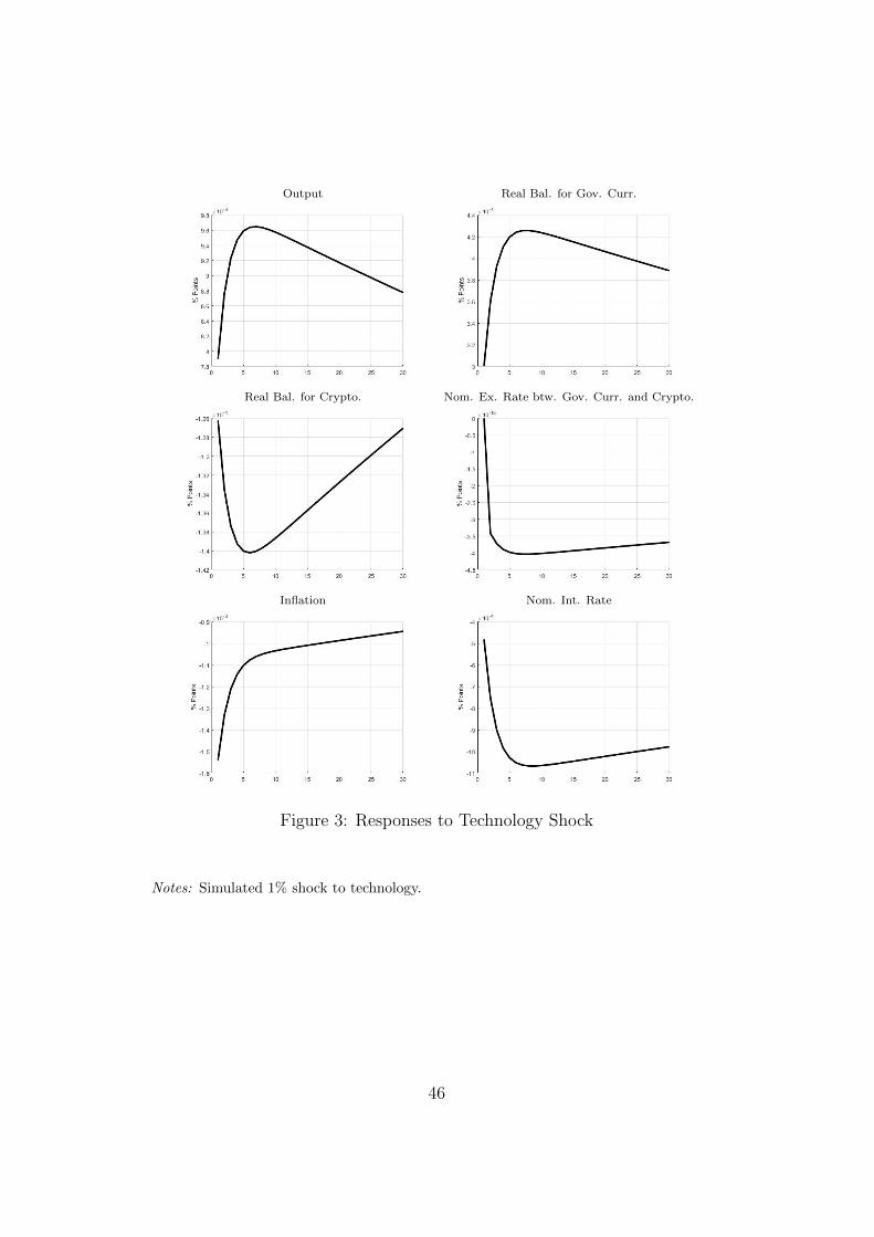
Output Real Bal. for Gov. Curr.

Real Bal. for Crypto. Nom. Ex. Rate btw. Gov. Curr. and Crypto.

Inflation Nom. Int. Rate

Figure 3: Responses to Technology Shock

Notes: Simulated 1% shock to technology.

46

Output Real Bal. for Gov. Curr.

Real Bal. for Crypto. Nom. Ex. Rate btw. Gov. Curr. and Crypto.

Inflation Nom. Int. Rate

Figure 4: Responses to Monetary Policy Shock

Notes: Simulated 1% shock to monetary policy.

47

Output Real Bal. for Gov. Curr.

Real Bal. for Crypto. Nom. Ex. Rate btw. Gov. Curr. and Crypto.

Inflation Nom. Int. Rate

Gov. Curr. Growth Gov. Curr. Dem. Shock

Crypto. Dem. Shock

Figure 5: Responses to Government Currency and Cryptocurrency DemandShocks

Notes: Simulated 1% shocks to government currency and cryptocurrency demands. Solidlines denote the responses to a government currency demand shock, whereas dashed linesrepresent the responses to a cryptocurrency demand shock.

48

Output Real Bal. for Gov. Curr.

Real Bal. for Crypto. Nom. Ex. Rate btw. Gov. Curr. and Crypto.

Inflation Nom. Int. Rate

Gov. Curr. Growth

Figure 6: Responses to Cryptocurrency Productivity Shocks

Notes: Simulated 1% shocks to common and specific productivity of cryptocurrency. Solidlines denote the responses to a common productivity shock of cryptocurrency, whereasdashed lines represent the responses to a specific productivity shock of cryptocurrency.

49

Cry

pto

.C

om

mon

Pro

d.

Sh

ock

Cry

pto

.S

pec

ific

Pro

d.

Sh

ock

Cry

pto

.C

om

mon

Pro

d.

Sh

ock

Cry

pto

.S

pec

ific

Pro

d.

Sh

ock

Ou

tpu

tR

eal

Bal.

for

Gov.

Cu

rr.

Rea

lB

al.

for

Cry

pto

.N

om

.E

x.

Rate

Infl

ati

on

Nom

.In

t.R

ate

Gov.

Cu

rr.

Gro

wth

Fig

ure

7:N

on-s

epar

abilit

yvs.

Sep

arab

ilit

y:

Res

pon

ses

toC

rypto

curr

ency

Com

mon

and

Sp

ecifi

cP

roduct

ivit

yShock

s

Notes:

Sim

ula

ted

1%sh

ock

toco

mm

onan

dsp

ecifi

cp

rod

uct

ivit

yof

cryp

tocu

rren

cy.

Soli

dli

nes

den

ote

the

IRF

sof

the

ben

chm

ark

mod

el,

wh

erea

sth

ed

ash

edan

dd

otte

dli

nes

rep

rese

nt

the

resp

on

ses

of

the

cou

nte

rfact

ual

mod

els

A(w

her

eω2

=0

an

dω3

=0)

an

dB

(wh

ere

ω3

=0)

,re

spec

tive

ly.

50

Output Real Bal. for Gov. Curr.

Real Bal. for Crypto. Nom. Ex. Rate btw. Gov. Curr. and Crypto.

Inflation Nom. Int. Rate

Gov. Curr. Growth

Figure 8: The Role of Monetary Policy: Responses to CryptocurrencyCommon Productivity Shock

Notes: Simulated 1% shock to common and specific productivity of cryptocurrency. Solidlines denote the IRFs of the benchmark model, whereas the dashed and dotted linesrepresent the responses of the model in scenarios 1 and 2, respectively.

51

Output Real Bal. for Gov. Curr.

Real Bal. for Crypto. Nom. Ex. Rate btw. Gov. Curr. and Crypto.

Inflation Nom. Int. Rate

Gov. Curr. Growth

Figure 9: The Role of Monetary Policy: Responses to CryptocurrencyCommon Productivity Shock

Notes: Simulated 1% shock to common and specific productivity of cryptocurrency. Solidlines denote the IRFs of the benchmark model, whereas the dashed and dotted linesrepresent the responses of the model in scenarios 1 and 2, respectively.

52

Table 1: Exogenous Shocks and Observed Variables

Shocks Observed Variables

Technology Shock US Industrial Production Index

Shock to Household’s Preferences US Real Private Consumption

Shock to Household’s Demand for Government Currency US Real Balances for Government Currency

Shock to Household’s Demand for Cryptocurrency Real Bitcoin Price

Common Productivity Shock of Cryptocurrency Real Cumulative Initial Coin Offering (ICO)

Specific Productivity Shock of Cryptocurrency Real Nvidia Volume Weighted Average Price

Monetary Policy Shock US Nominal Interest Rate

Notes: The data sources and the construction of all observed variables are reported inAppendix B.

53

Table 2: Priors and Posteriors for the Endogenous Parameters

Parameter Symbol Priors Posteriors

Dist. Mean St. Dev. Mean Conf. Inter.

Output El. to Real Bal. of Gov. Currency ω2 G 0.200 0.050 0.195 0.102 0.284

Output El. to Real Bal. of Cryptourrency ω3 G 0.050 0.010 0.035 0.024 0.046

Income El. of Gov. Currency Demand γ1 G 0.015 0.005 0.021 0.009 0.032

Interest Semi-El. of Gov. Currency Demand γ2 G 0.150 0.050 0.140 0.066 0.214

El. of Real Bal. of Gov. Curr. wrt Gov. Curr. Dem. Shock γ3 G 0.900 0.100 0.664 0.593 0.733

Cross El. of Gov. Cur. Dem. and Crypto. Dem. γ4 G 0.500 0.050 0.554 0.467 0.638

Income El. Cryptocurrency Demand γ5 G 0.015 0.005 0.013 0.006 0.020

Interest Semi-El. of Cryptocurrency Demand γ6 G 0.150 0.050 0.155 0.073 0.236

El. of Real Bal. of Crypto. wrt Crypto. Dem. Shock γ7 G 0.800 0.100 1.034 1.014 1.053

Cross El. of Crypto. Dem. and Gov. Cur. Dem. γ8 G 0.600 0.100 1.011 0.985 1.037

Ex. Rate Crypto. / Gov. Cur. El. wrt Prod. % G 0.900 0.100 0.777 0.638 0.916

Share of Crypto. Common Prod. on Crypto. Tot. Prod. ξφ G 0.500 0.050 0.572 0.482 0.662

Interest. Rate Smoothing ρr B 0.800 0.050 0.808 0.765 0.852

Taylor Rule Coef. on Output ρy B 0.200 0.010 0.153 0.142 0.163

Taylor Rule Coef. on Inflation ρπ G 1.800 0.050 1.980 1.900 2.063

Taylor Rule Coef. on Gov. Currency Growth ρµg

B 0.200 0.050 0.459 0.368 0.555

Table 3: Priors and Posteriors for the Shock Processes Parameters

Parameter Symbol Priors Posteriors

Distr. Mean St. Dev. Mean Conf. Inter.

Household’s Preference Shock Pers. ρa B 0.700 0.050 0.668 0.586 0.751

Gov. Cur. Demand Shock Pers. ρeg B 0.650 0.050 0.623 0.548 0.700

Crypto. Demand Shock Pers. ρec .B 0.550 0.050 0.622 0.554 0.690

Technology Shock Pers. ρz B 0.900 0.050 0.996 0.992 0.999

Crypto. Common Prod. Shock Pers. ρξ B 0.600 0.050 0.679 0.616 0.742

Crypto. Specific Prod. Shock Pers. ρν B 0.600 0.050 0.703 0.642 0.765

Household’s Preference Shock St. Err. σa I-G 0.010 Inf 0.278 0.238 0.315

Gov. Cur. Demand Shock St. Err. σeg I-G 0.010 Inf 1.578 0.824 2.320

Crypto. Demand Shock St. Err. σec I-G 0.010 Inf 3.799 3.065 4.538

Technology Shock St. Err. σz I-G 0.010 Inf 0.734 0.611 0.853

Crypto. Common Prod. Shock St. Err. σξ I-G 0.010 Inf 0.047 0.041 0.054

Crypto. Specific Prod. Shock St. Err. σν I-G 0.010 Inf 4.763 4.071 5.436

Monetary Policy Shock St. Err. σr I-G 0.010 Inf 0.076 0.059 0.091

54

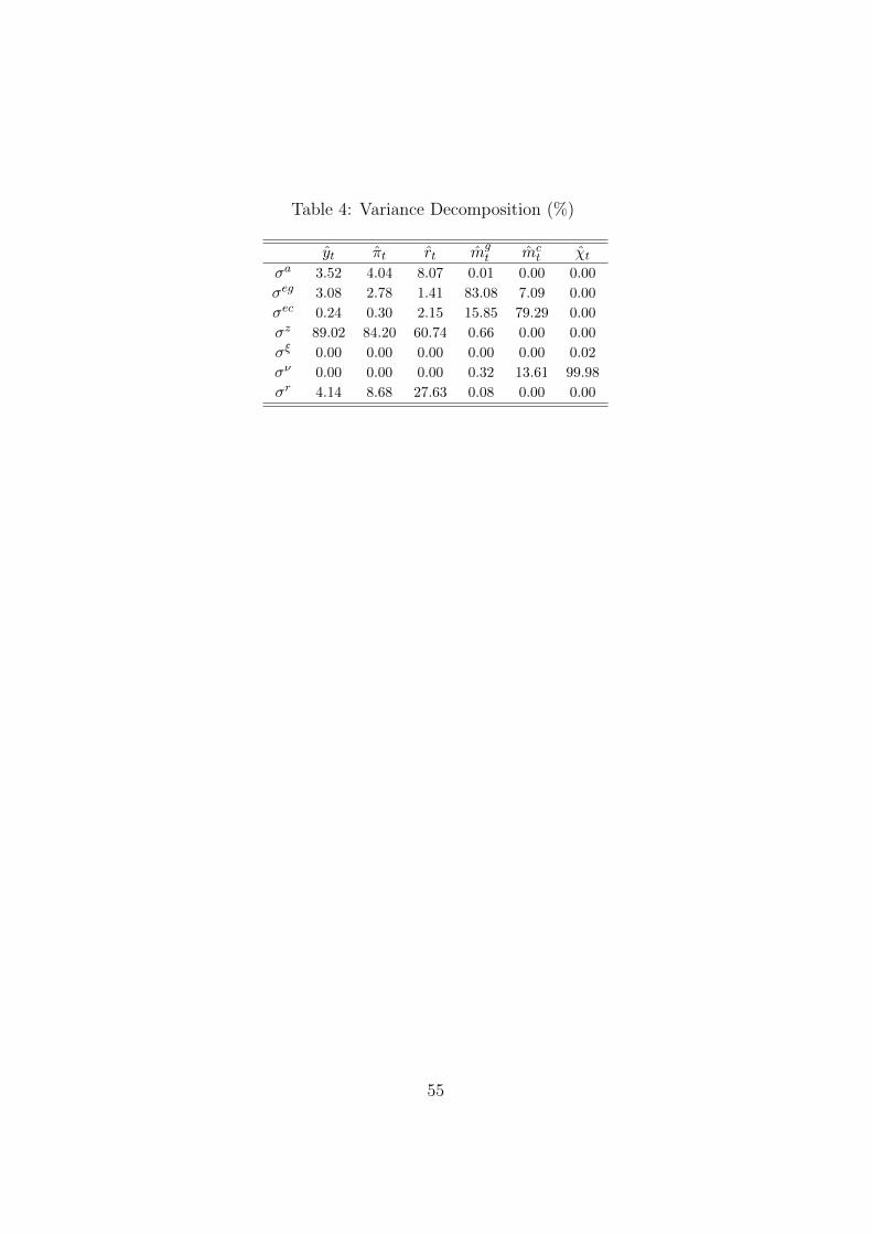
Table 4: Variance Decomposition (%)

yt πt rt mgt mc

t χtσa 3.52 4.04 8.07 0.01 0.00 0.00

σeg 3.08 2.78 1.41 83.08 7.09 0.00

σec 0.24 0.30 2.15 15.85 79.29 0.00

σz 89.02 84.20 60.74 0.66 0.00 0.00

σξ 0.00 0.00 0.00 0.00 0.00 0.02

σν 0.00 0.00 0.00 0.32 13.61 99.98

σr 4.14 8.68 27.63 0.08 0.00 0.00

55

Table 5: Forecast Error Variance Decomposition (%)

Period 1

yt πt rt mgt mc

t χtσa 6.41 4.82 6.68 0.00 0.00 0.00

σeg 5.49 2.41 1.29 83.45 7.17 0.00

σec 0.41 0.25 1.97 15.86 80.23 0.00

σz 80.49 82.69 28.03 0.30 0.00 0.00

σξ 0.00 0.00 0.00 0.00 0.00 0.02

σν 0.01 0.00 0.00 0.29 12.60 99.98

σr 7.19 9.82 62.04 0.09 0.00 0.00

Period 5

yt πt rt mgt mc

t χtσa 1.48 1.84 6.04 0.01 0.00 0.00

σeg 1.38 1.72 1.02 82.39 7.02 0.00

σec 0.08 0.12 1.56 15.76 78.35 0.00

σz 95.14 91.69 75.72 1.43 0.00 0.00

σξ 0.00 0.00 0.00 0.00 0.00 0.02

σν 0.00 0.00 0.00 0.34 14.62 99.98

σr 1.91 4.63 15.65 0.08 0.00 0.00

Period 12

yt πt rt mgt mc

t χtσa 0.59 0.99 2.54 0.01 0.00 0.00σeg 0.55 0.95 0.42 80.39 7.00 0.00σec 0.04 0.07 0.64 15.38 78.11 0.00σz 98.06 95.49 90.49 3.81 0.00 0.00σξ 0.00 0.00 0.00 0.00 0.00 0.02σν 0.00 0.00 0.00 0.34 14.89 99.98σr 0.76 2.49 5.92 0.07 0.00 0.00

Period 30

yt πt rt mgt mc

t χtσa 0.25 0.49 1.03 0.01 0.00 0.00

σeg 0.23 0.46 0.17 76.08 7.00 0.00

σec 0.01 0.03 0.26 14.56 78.10 0.00

σz 99.19 97.80 96.13 8.97 0.01 0.00

σξ 0.00 0.00 0.00 0.00 0.00 0.02

σν 0.00 0.00 0.00 0.32 14.89 99.98

σr 0.32 1.22 2.41 0.07 0.00 0.00

56

Table 6: Posterior Estimates for the Endogenous Parameters - BenchmarkModel vs. Counterfactual Models A and B

Parameter Symbol Benchmark Counterfactual A Counterfactual Bwith ω2 = 0 and ω3 = 0 with ω3 = 0

Mean Conf. Int. Mean Conf. Int. Mean Conf. Int.

Output El. to Real Bal. of Gov. Currency ω2 0.195 0.102 0.284 - - - 0.241 0.154 0.326Output El. to Real Bal. of Cryptourrency ω3 0.035 0.024 0.046 - - - - - -

Income El. of Gov. Currency Demand γ1 0.021 0.009 0.032 0.015 0.007 0.022 0.017 0.008 0.025Interest Semi-El. of Gov. Currency Demand γ2 0.140 0.066 0.214 0.151 0.070 0.228 0.137 0.064 0.209

El. of Real Bal. of Gov. Curr. wrt Gov. Curr. Dem. Shock γ3 0.664 0.593 0.733 0.948 0.786 1.114 0.716 0.621 0.804Cross El. of Gov. Cur. Dem. and Crypto. Dem. γ4 0.554 0.467 0.638 0.483 0.404 0.561 0.515 0.432 0.597

Income El. Crypto. Demand γ5 0.013 0.006 0.020 0.015 0.007 0.023 0.014 0.007 0.022Interest Semi-El. of Crypto. Demand γ6 0.155 0.073 0.236 0.149 0.068 0.226 0.158 0.074 0.241

El. of Real Bal. of Crypto. wrt Crypto. Dem. Shock γ7 1.034 1.014 1.053 0.998 0.981 1.015 1.006 0.992 1.019Cross El. of Crypto. Dem. and Gov. Cur. Dem. γ8 1.011 0.985 1.037 1.012 0.969 1.055 1.007 0.975 1.039

Ex. Rate Crypto. / Gov. Cur. El. wrt Prod. % 0.777 0.638 0.916 0.795 0.651 0.935 0.796 0.654 0.935

Share of Crypto. Common Prod. on Crypto. Tot. Prod. ξφ 0.572 0.482 0.662 0.558 0.471 0.646 0.559 0.471 0.647

Interest. Rate Smoothing ρr 0.808 0.765 0.852 0.801 0.757 0.847 0.804 0.761 0.849Taylor Rule Coef. on Output ρy 0.153 0.142 0.163 0.153 0.142 0.163 0.153 0.142 0.163Taylor Rule Coef. on Inflation ρπ 1.980 1.898 2.063 1.987 1.904 2.071 1.985 1.902 2.068

Taylor Rule Coef. on Gov. Currency Growth ρµg

0.459 0.368 0.555 0.448 0.352 0.545 0.456 0.363 0.553

57