A Mixed-Regime Model for Dry Bulk Freight Market

185

The Asian Journal of Shipping and Logistics ● Volume 26 Number 2 December 2010 pp. 185-204●

A Mixed-Regime Model for Dry Bulk Freight Market1)*

Byoung-wook KO2)**

Contents

I . Introduction IV. Analysis of Empirical Results and II . Literature Review Interpretations III. Empirical Model and Data V. Conclusion

Abstract

This paper constructs a mixed-regime model for dry bulk freight market. Then it performs maximum likelihood estimation and provides the results. Inter alia, the hypothesis that there is bimodality in the supply curve of shipping freight markets is strongly supported by analyzing the effect of the term structure of time-charter rates on the time-varying volatility.

Furthermore, the adjustment speed of 1-year time-charter rate in low-volatility regime is larger than in high-volatility regime, which means the market players consider the backwardation shock in low uncertainty as more important than in high uncertainty. Especially the Cape-size markets respond positively to the back-wardation shock in low-volatility regime but respond negatively in high-volatility regime. Finally, the estimated time-varying variance using real-time data has a highly statistically significant relation with the next squared error terms.

Key words : mixed-regime model, term structure of time-charter rates, time-varying volatility

* The author greatly appreciates Prof. Chang-Jin Kim for his invaluable encouragement and helpful comments on the topics of this paper. Also, the suggestions of the three anonymous referees are very helpful for the improvement of the paper. However, the author is responsible for the remaining errors of this paper.** Senior Researcher of Korea Maritime Institute, Korea, Email : [email protected]

186

A Mixed-Regime Model for Dry Bulk Freight Market

I. Introduction

It is well-known that there has been a remarkable increase of volatility in dry bulk freight market since mid-2003. (See <Figure 1>) Especially, the recent global financial shock and its effect showed that there could be a sudden collapse in overall economic activity, which lead to 96% BDI (Baltic Dry Index) drop in a few months. For most of incumbent shipping suppliers, this volatility is very painful mainly because the unanticipated big drop in earnings and its lasting low level push them into significant deficit. Moreover, even though possible, the anticipation of volatility leads to high risk premium. From other viewpoints of investors, financial intermediaries, this volatility is harmful in the sense that their asset is exposed to high risk.

Therefore, due to the importance of managing the risk from the high volatility, there have been numerous attempts to model the variance of earnings in shipping market.1) For example, Alizadeh and Nomikos (2010) measured additional asymmetric impact on the volatility in the different market conditions by using a cubic function of the slope of the forward curve, which was calculated by the difference between the log of spot and log of three-year time-charter earnings.2) According to their results, there is statistically significant effect of the shape of freight term structure on the volatility in most of the considered cases.

However, relatively few studies have made to assume that there are some different regimes of volatility in shipping market and the regime may depend on the observable market information. This paper aims to characterize the bulk freight market by modeling a mixed-regime dynamics. Through this approach, we will verify empirically the hypothesis that there is significant effect of time-charter market condition on the volatility of the market as in Alizadeh and Nomikos and show that the adjustment speed of 1-year time-charter rate in low-volatility regime is larger than in high-volatility regime, which means that the market players consider the backwardation shock in low uncertainty as more important than in high uncertainty. The latter

1) See Kavussanos (1996); Chen and Wang (2004); Jing et al. (2008); Alizadeh and Nomikos (2010).2)Alizadeh and Nomikos (2010).

187


finding makes this paper different from the previous literature which has not considered the different regimes.

The organization of this paper is as follows: Section 2 reviews the relevant literature focusing on the heteroskedasticity and the term structure of dry bulk freight market. Section 3 proposes an empirical mixed-regime model whose regimes are independent each other and explains the data set. Section 4 reports the estimation results and provides implications and discussion points. Finally, section 5 summarizes the paper and suggests some future research topics.

<Figure 1> Baltic Dry Index (BDI)

Source : Clarkson

II. Literature Review

This paper considers the time-varying volatility model for dry bulk freight market. This variability of volatility means that there is time-varying risk.3) Facing with the heteroskedasticity, a number of papers attempt to model the shipping market dynamics with GARCH-type one.4) Among others,

3) For a recent thorough discussion on freight risk management and FFA (Forward Freight Agreement) trading, see Alizadeh and Nomikos (2009).4) GARCH (Generalized Auto-Regressive Conditional Heteroskedasticity) model was a general version of ARCH (Auto-Regressive Conditional Heteroske- dasticity) model. ARCH model was introduced by Engle (1982). Bollerslev (1986) proposed GARCH model, arguing that the ARCH models can be over-parameterized.

Kavussanos used ARCH and GARCH models to investigate the time-varying volatility for different-type vessels and different-period contracts of dry shipping markets.5)

More recently, researchers have used EGARCH (Exponential GARCH) model, which was proposed in Nelson.6) Using this model, Chen and Wang found that the daily return of three different markets (i.e., Cape, Panamax, and Handymax) showed a significantly negative relation in terms of return and volatility and the leverage effect on volatility7) is more significant in market downward movement than in market upward movement under the same magnitude of innovation. Furthermore, the larger vessels have much more leverage effect than smaller vessels contemporaneously. Jing et al.8) also investigated the asymmetric impact between past innovations and current volatility by using EGARCH model. Alizadeh and Nomikos investigated the effect of the term structure on the time-varying volatility of (bulk and tanker) freight markets. Especially, by inserting a cubic function of the slope of term structure into the conditional variance, they showed that the freight rate volatility increases in a backwardated market and decreases when the market is in contango.

Relating to the issue of term structure of freight market with different contract-period, there have been a number of researches. Many of them studied the risk premium, which implied by the term structure. Kavussanos and Alizadeh9) tested the expectations hypothesis of the term structure (EHTS) by using various test techniques. On rejecting EHTS, they attributed this failure to shipowners’ perceptions of time-varying risk regarding their decision to operate in spot or time charter markets. Adland and Cullinane10) suggested a simple logical argument based on maritime economic theory in which the inherent risks in shipping market are 1) spot market volatility, 2) utilization risk, 3) the risk of transport shortage, 4) default risk, 5) liquidity risk, 6) technological or regulatory obsolescence. They also argued that these

5) Karussanos (1996).6) Nelson (1991).7) The meaning of the leverage effect is that risk-adverse investors respond much faster to negative returns than to positive returns. See Black (1976) p. 2 for original statement and Chen and Wang (2004) p. 121.8) Jing et al (2008).9) Kavussanos and Alizadeh (2002).10) Adland and Cullinane (2005).

188


various risks make the expectations hypothesis rejected. However, Wright11) argued that the difference between the short-period and long-period freight rates should be carefully interpreted. That is, since there is the possibility that the markets with different contract-period are segmented by the idiosyncratic supply and demand characteristics,12) the time-varying risk premium, measured by the difference between the short-period and long-period freight rates, may have no theoretical significance.

Recently, Angelidis and Skiadopoulos13) evaluated the performance of different models to determine Value-at-Risk (VaR) for shipping freight rate positions. According to the results, they found no significant evidence in favor of sophisticated methods and concluded that the simple Historical simulation (HS) one is good enough to yield relatively accurate VaR estimates.

As some other approaches to understanding the shipping freight markets, Engelen et al.14) used a multi-agent system dynamics model and Koekebakker and Adland15) constructed a continuous time model in Heath-Jarrow-Morton framework.

III. Empirical Model and Data

The changing volatility of data over time can be modeled by various approaches as discussed in the previous section. However, this paper attempts to capture the dynamic properties of dry bulk freight market by using a mixed-regime model with heteroskedasticity.

In the mixed-regime model of this paper, there are two different extreme regimes with low and high variance and the state at a given time can be a mixture of different regimes, the mixing way of which can evolve. By dividing the actual state into the low-volatility and high-volatility regimes, we can characterize the market differently from (E)(G)ARCH model and then

11) Wright (2007).12) This segmentation hypothesis is based on the concept of so-called ‘preferred habitat’.13) Angelidis and Skiadopoulos(2008).14) Engelen et al. (2008).15) Kokeke Bakker and Adland (2004).

189


190


extract some useful information.16) This approach of mixed-regime stems from so-called regime-switching model. A brief history of the literature of independent regime switching model is as follows.

Quandt17) showed that there had been various kinds of switching models and then proposed so-called λ-method as an alternative. According to the λ-method, we may think of nature choosing regimes 1 and 2 with unknown probabilities λ and 1-λ. Goldfeld and Quandt18) explained λ-method under the label ‘stochastic choice of regimes’ and the D-method under the deterministic switching. They suggested that the probability λ in the λ-method itself can be a function of some other variable and the resulting procedure is a hybrid between the D-method and λ-method. Goldfeld and Quandt compared the performances of LS (least squares) and ML (Maximum likelihood) estimations and concluded MLE appeared to be distinctly preferable, partly because MLE uses some additional information.

For the mechanism to yield the probability of the state at time t, Goldfeld and Quandt used the cumulative normal distribution function. However, this paper uses a specification similar with that of p. 62 of Kim and Nelson.19) The selection of more appropriate mechanism to yield the state probability remains as a future research topic.

The following mixed-regime (or regime-switching) model can be considered:

(1) (2) (3) (4)

(5) (6)

16) For example, we can investigate the determinants of time-varying volatility, different market characteristics across different regimes, and so on. A rationale of this approach can be suggested as follows: For the convenience of perception, we often consider some extreme cases or analyze a situation by assuming strong assumptions at first. Then we may think that the reality is at a point on the spectrum between the extreme cases or understand the reality by relaxing some assumptions.17) Quandt (1972).18) Goldfeld and Quandt (1973).19) Kim and Nelson (1999) .

As mentioned in Kim and Nelson, if we know the dates of regime switching, the state-governing variable, St, becomes a simple dummy.

However, a major problem emerges because we cannot know its date exactly. For the problem which the paper aims to solve, the state of the equations (1) to (4) may be considered as a weighted average state and their weights can become the probabilities at the time over the evolution path, {pt}.

Kim and Nelson suggest a solution to estimating the value of pt as follows:

Step 1. First, consider the joint density of yt and the unobserved St variable, which is the product of the conditional and marginal densities:

(7)

where It-1 refers to information up to time t-1.

Step 2. Then, to obtain the marginal density of yt, integrate the St variable out of the above joint density by summing over all possible values of St:

(8)

Based on the equation (8), we can construct the (log) likelihood function, which makes it possible to estimate the parameters by Maximum Likelihood Estimation (MLE). The equations (5) and (6) postulate that the regimes

191


depend on the predetermined variables, X΄t-1 which can include the information on the term structure of time charter rates, past volatility, etc.

When practicing MLE, for technical reason of estimation, we set the lower bound, 0.0025, for the low variance, σ²0.

The considered dry bulk markets can be classified into 1) Cape-size, 2) Panamax-size, 3) Handymax-size markets by the ship size and also classified into 1) spot, 2) 6-month time-charter, 3) 1-year time-charter, 4) 3-year time-charter markets by the contract period. Therefore, they are all 12 separate ones.20) The explanation of data is suggested in <Table 1>. The period of data is from 31st January 1992 to 28th May 2010. Because the variable of past volatility belongs to the explanatory variable and its calculation requires one-year observations, the estimation period becomes from 5th February 1993 to 28th May 2010. Based on the maximum number of lags of Alizadeh and Nomikos,21) this paper sets the lag number as 3 basically.

<Table 1> Data explanations of spot and time-charter rates

Spot 6-month, 1-year, 3-year

Cape-size 1990/91-built, Average spot earnings 150,000 dwt Bulkcarrier time-charter rates

Panamax-size 1980s-built, Average spot earnings 65,000 dwt Bulkcarrier time-charter rates

Handymax-size 45,000 dwt, Average trip earnings 45,000 dwt Bulkcarrier time-charter rates

Note: The unit of all the rates is $/day.Source: Clarkson

In all markets of different size, the spot earning is above that of 3-year on average as shown in <Table 2>. This fact means that, in contrast to the financial market, there is negative risk premium to the ship owner (i.e., the lender of ship) on average. Also, in the aspect of volatility, the spot market is more volatile than the 3-year time-charter market.

21) Some literature considers the relationship among them. (For example, see Chen et al. (2010)) However, this paper doesn’t deal with this kind of relationship. The study on it remains as future research topic.21) Alizadeh and Nomikos (2010)

192


<Table 2> Descriptive statistics of freight earnings for different types of vessels in the dry market

Unit : US$/day

Spot 6-month 1-year 3-year

Capemean 30,137 30,683 28,895 24,215

standard deviation 29,419 30,976 27,859 18,693

Panamaxmean 15,929 16,107 14,893 11,785


Handymaxmean 15,473 15,633 14,733 12,457


The variable, rt , is measured by the percentage change22) during the unit period which is one week in most of the cases. It can be 1) spot rate, 2) 6-month, 3) 1-year, or 4) 3-year time-charter rate, respectively. The unconditional mean and standard deviation of the rates of these markets across different period are shown <Table 3>.

Zt-1 represents the condition of time-charter markets. As well explained in Alizadeh and Nomikos, when the short-period rate is above the long-period one (in backwardation), we can think that the market is in the area of inelastic supply curve. So, the rate variation from the change of demand would be larger in backwardation than in opposite condition (in contango). In order to measure the time-charter market condition, this paper uses the ratio of the difference between 6-month rate and 3-year rate to 6-month one at time t-1.23)

X΄t-1 includes Zt-1 and the past volatility, as in usual (G)ARCH-type model. But the specific measure for past volatility is different from (G)ARCH-type

one. This paper uses the ratio of the standard deviation in last 4 weeks to that in the last entire weeks as a proxy for unconditional past volatility, which is

denoted by .

22) Many econometric literatures use the change rate calculated by the log difference. However, this paper calculated the change rate by the ratio of the change over the level, which is used mostly in our actual life. Its reason is simply that the proposed model can provide a practical tool for measuring a volatility used in real life.23) By dividing the difference by the rate level, we can more exactly measure the time-charter market condition. For a different method, we may use a log difference of the related rates.

193


<Table 3> Unconditional mean and volatility of rate change for different size ships over different sample periods

Spot 6-month 1-year 3-yearCape-size

Feb. 93 toJune 03

mean 0.32 0.37 0.23 0.11standard deviation 5.63 5.51 3.84 2.90

July 03 toAug. 08


Sep. 08 toFeb. 09

mean 0.80 1.14 -2.80 -2.00standard deviation 36.23 47.17 25.76 25.88

March 09to May 10


Panamax-size

Feb. 93 toJune 03


July 03 toAug. 08


Sep. 08 toFeb. 09

mean 4.46 -3.46 -5.47 -3.44standard deviation 53.45 26.58 16.72 15.31

March 09to May 10


Handymax-size

Feb. 93 toJune 03


July 03 toAug. 08


Sep. 08 toFeb. 09

mean -1.74 -3.73 -4.28 -3.24standard deviation 22.97 15.35 11.53 10.53

March 09to May 10


194


IV. Analysis of Empirical Results and Interpretations

First of all, as shown in Alizadeh and Nomikos (2010), the term structure of time-charter rates effects on the volatility in most of the samples. That is, there is highly statistically significant effect of time-charter market condition on the volatility of the market. (See the estimates of coefficient and its t-value of p1,1 in Tables <4~6>), although there is one exceptional case of Handymax 1-year before July 2003.24) The positive sign means that an increase in the extent of backwardation condition leads to more volatility in the spot and time-charter rates.25)) Of course, this empirical evidence supports the hypothesis that there is bimodality in the supply curve of shipping freight markets. That is, the shipping service supply curve is elastic in excess of capacity, but it is inelastic in excess of demand. However, Alizadeh and Nomikos used a cubic term but this paper uses a simple linear probability function for the effect of term structure on the volatility. Thus, the nonlinearity of the relationship between the term structure and market volatility is needed to be tested, which remains as a future research topic.

<Figure 2> Bimodality in shipping freight market

Source : Alizadeh and Nomikos (2010)

24) For simplicity, γst is assumed to be the same between the regimes.25) By contrast, Alizadeh and Nomikos (2010) showed that there is no statistically significant effect in Panamax spot market.

195


<Table 4> Estimation results of Cape-size markets

Model :


α1

Whole sample 0.33***(8.89) 0.07***(3.20) 0.07***(3.20) 0.00(0.004)

Pre July 03 0.43***(9.64) 0.10***(3.11) 0.10***(3.41) 0.00(0.02)

Post July 03 0.16***(3.53) 0.08**(1.93) 0.09***(2.95) 0.00(0.002)

α2

Whole sample 0.03(1.15) 0.05***(4.00) 0.05***(4.00) 0.00(0.01)

Pre July 03 -0.03(-0.88) 0.009(0.33) 0.07***(2.47) 0.00(0.01)

Post July 03 0.11***(2.70) 0.04**(1.29) 0.04*(1.48) 0.00(0.005)

α3

Whole sample - 0.04***(3.60) 0.04***(3.60) 0.00(0.01)

Pre July 03 0.04(1.10) 0.07**(2.08) 0.05**(2.02) 0.00(0.01)

Post July 03 - 0.04**(1.78) 0.03*(1.28) 0.00(0.005)

γ

Whole sample - -0.52(-1.01) -0.52(-1.01) 0.00(0.001)

Pre July 03 -0.55(-0.80) -0.12(-0.31) -0.14(-0.39) 0.00(0.001)

Post July 03 - -0.76(-0.60) 1.19(1.27) -

p0

Whole sample 3.79**(1.88) 6.01***(3.38) 6.01***(3.38) 6.51***(19.71)

Pre July 03 6.34(0.77) 9.18***(5.69) 9.32***(4.45) 5.59***(8.86)

Post July 03 -6.09***(-2.41) 2.66(0.62) 3.26(0.56) 8.20***(5.96)

p1,1

Whole sample 6.73***(7.80) 6.71***(9.17) 6.71***(9.17) 10.13***(41.29)

Pre July 03 4.61**(1.77) 13.1***(7.27) 11.30***(6.17) 13.86***(24.64)

Post July 03 3.99***(3.27) 2.23***(3.09) 3.81***(4.88) 8.68***(12.06)

p1,2

Whole sample 7.77***(5.46) 5.13***(3.72) 5.13***(3.72) 6.84***(21.73)

Pre July 03 0.88(0.08) 1.37(0.94) 7.50***(4.15) 18.14***(25.13)

Post July 03 5.88***(2.88) 7.54***(3.08) 5.39***(2.64) 4.97***(3.68)

σ²0

Whole sample 18 10 10 0.0025

Pre July 03 13 4 2 0.0025

Post July 03 70 35 20 0.0025

σ²1

Whole sample 356 511 511 97

Pre July 03 116 61 31 11

Post July 03 945 1149 454 209

Note: *, ** and *** indicate significance at 10%, 5% and 1% levels, respectively.

196


<Table 5> Estimation results of Panamax-size markets

Model :


α1

Whole sample 0.33***(10.92) 0.04*(1.52) 0.07***(2.45) 0.00(-0.0001)

Pre July 03 0.37***(8.35) 0.10***(2.90) 0.17***(4.51) 0.00(0.03)

Post July 03 0.40***(7.93) -0.02(-0.43) 0.01(0.34) 0.00(-0.0008)

α2

Whole sample 0.007(0.34) 0.02(0.63) 0.06**(1.69) 0.00(0.01)

Pre July 03 -0.04(-0.93) 0.02(0.81) 0.04(1.25) 0.00(0.006)

Post July 03 -0.09***(-2.67) 0.07**(1.64) 0.07**(1.66) 0.00(0.007)

α3

Whole sample -0.09***(-4.45) 0.03(0.85) 0.03(1.18) 0.00(0.02)

Pre July 03 -0.11***(-2.60) 0.04(1.25) - 0.00(-0.01)

Post July 03 0.05(1.26) 0.09(1.90) 0.12***(3.27) 0.00(0.01)

γ

Whole sample - 0.37(0.66) 0.70*(1.50) 0.00(0.01)

Pre July 03 0.87(0.73) -0.89(-0.78) - 0.0004(0.026)

Post July 03 - 0.40(0.50) - 0.00(0.004)

p0

Whole sample -1.52(-0.95) 1.42*(1.75) 0.89(0.82) 4.74***(13.51)

Pre July 03 -19.85***(-679.74) 3.92(1.04) -1.35(-0.46) 20.33***(11.44)

Post July 03 -4.38***(-3.10) -11.98***(-3.21) -8.50***(-2.65) 3.98(0.90)

p1,1

Whole sample 4.92***(5.97) 8.38***(10.15) 7.22***(9.12) 10.63***(35.37)

Pre July 03 3.27***(75.11) 10.28***(4.01) 7.50***(4.43) 12.73***(16.15)

Post July 03 2.02***(3.60) 3.07***(3.71) 1.64***(3.09) 9.04***(13.57)

p1,2

Whole sample 3.02***(4.82) 11.26***(9.14) 11.73***(7.92) 6.16***(16.59)

Pre July 03 42.54***(208.08) 11.75***(2.85) 20.39***(4.57) 11.67***(6.32)

Post July 03 4.91***(3.41) 14.66***(4.32) 15.04***(4.71) 3.13**(1.95)

σ²0

Whole sample 25 9 5 0.0025

Pre July 03 13 7 3 0.0025

Post July 03 65 36 18 0.0025

σ²1


Pre July 03 71 71 32 10

Post July 03 2032 494 331 150


197


<Table 6> Estimation results of Handymax-size markets

Model :


α1

Whole sample 0.44***(13.72) 0.25***(9.88) 0.20***(6.89) 0.0002(0.16)

Pre July 03 0.39***(9.65) 0.19***(5.04) 0.002(0.11) 0.0002(0.09)

Post July 03 0.53***(11.29) 0.30***(5.92) 0.23***(6.03) 0.16***(5.16)

α2

Whole sample -0.03*(-1.43) 0.02(0.76) 0.04*(1.37) 0.0001(0.12)

Pre July 03 0.07**(1.85) 0.06**(1.92) 0.002(0.09) 0.00(0.02)

Post July 03 -0.06**(-1.66) 0.04(0.88) 0.03(0.46) 0.06**(2.04)

α3

Whole sample 0.03(1.00) 0.03**(1.86) 0.006(0.14) 0.00(0.01)

Pre July 03 0.04(1.13) 0.02(0.86) 0.00(0.03) 0.00(0.005)

Post July 03 -0.05*(-1.34) 0.002(0.02) -0.001(-0.009) 0.04**(1.80)

γ

Whole sample -0.03(-0.43) 0.11(0.14) 0.37(1.24) -0.0002(-0.01)

Pre July 03 - -0.53(-0.94) -0.0002(-0.007) 0.0008(0.03)

Post July 03 0.19(0.30) 0.87*(1.52) 0.39(0.71) 0.85***(3.08)

p0

Whole sample -1.07(-0.53) 5.26***(4.36) 5.86***(3.59) 11.31***(37.52)

Pre July 03 8.15**(1.69) 22.46***(4.06) 57.87***(14.94) 22.95***(18.42)

Post July 03 -19.10***(-3.50) 0.40(0.05) 0.76(0.06) -6.18*(-1.32)

p1,1

Whole sample 8.21***(8.12) 8.54***(8.95) 9.11***(9.36) 12.80***(46.35)

Pre July 03 8.67***(3.85) 11.11***(4.38) -0.13(-0.09) 22.18***(18.93)

Post July 03 4.47***(4.39) 2.49***(3.12) 2.84***(3.06) 7.34***(6.67)

p1,2

Whole sample 11.59***(5.94) 7.07***(4.67) 8.65***(4.94) 9.19***(32.26)

Pre July 03 14.35***(2.66) 0.92(0.18) -2.75(-0.62) 8.22***(9.68)

Post July 03 12.52***(4.06) 9.61*(1.54) 9.55**(2.30) 9.59*** (4.25)

σ²0

Whole sample 3 2 1 0.0025

Pre July 03 1 1 0.0025 0.0025

Post July 03 13 8 5 1

σ²1


Pre July 03 13 16 4 3

Post July 03 329 173 108 51


198


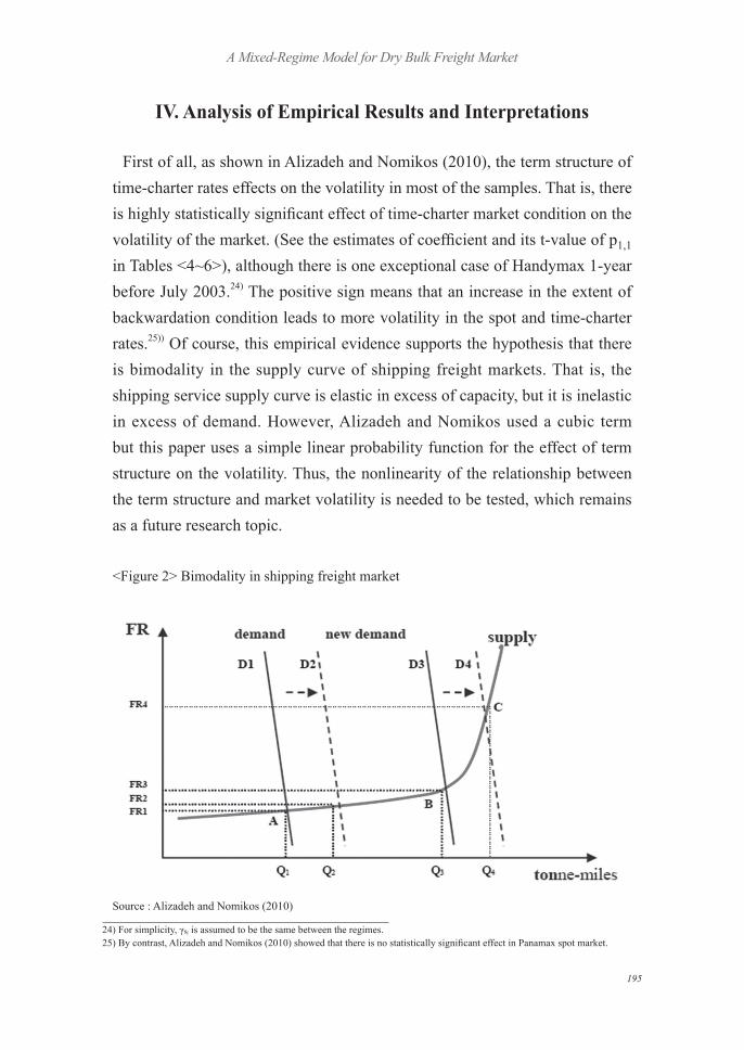
Secondly, the adjustment speed of 1-year time charter26) would be somewhat different between the low and high volatility regimes. (See the estimates of γ0 and γ1 ) That is, 6 cases out of 9, the adjustment speed in low-volatility regime is larger than in high-volatility regime, which means that the market players consider the backwardation shock in low uncertainty as more important than in high uncertainty.27) Especially, the Cape-size markets show that the 1-year time-charter markets respond positively to the backwardation shock in low-volatility regime but respond negatively in high-volatility regime, although the statistical significance is low. Furthermore, this tendency becomes stronger since July 2003. This kind of information about behavior change in the 1-year charter market would be helpful for the market participants and also implies that there would have been some structural change, for example, in the decision making process of market participants. Interestingly, before July 2003, the Handymax 1-year time-charter market showed the opposite pattern to that of Cape market.

The above empirical finding is derived from the univariate AR(p) specification. However, the measure for adjustment speed is well explained in the framework of ‘cointegration relationship’, which means that the multivariate specification is more appropriate in this kind of research. More specifically, VECM (Vector-autoregressive Error Correction Model) with mixed-regime volatility would be productive in understanding the considered markets, which also remains as a future research topic.

Thirdly, in order to check the forecasting power of time-varying variance, we perform a regression analysis as follows:

(9)

26) This is the effect of time-charter market condition on the level of dependent variables, not on its volatility.27) This finding is an essential contribution of this paper using a mixed-regime model.

199


<Table 7> Estimation results of adjustment speed of 1-year market

Model :

Cape-size Panamax-size Handymax-size

α1

Whole sample 0.04***(2.90) 0.08***(2.81) 0.22***(9.07)

Pre July 03 0.09***(2.68) 0.17***(4.30) 0.0003(0.14)

Post July 03 0.09***(2.73) 0.04(1.05) 0.25***(6.68)

α2

Whole sample 0.02*(1.45) 0.05*(1.61) -

Pre July 03 0.06**(1.82) 0.04(1.16) -

Post July 03 0.05**(1.70) 0.04(0.97) -

α3

Whole sample 0.02**(2.11) - -

Pre July 03 0.04**(1.70) - -

Post July 03 - - -

γ

Whole sample 0.31(1.00) 0.59(1.11) 0.46*(1.49)

Pre July 03 0.03(0.32) 0.31(0.28) -0.0008(-0.03)

Post July 03 1.58*(1.63) 0.09(0.25) 0.47(0.91)

γ1

Whole sample -0.75(-0.46) 1.24(0.68) 0.44(0.42)

Pre July 03 -1.72(-1.19) -0.85(-0.27) 1.55*(1.52)

Post July 03 -5.17(-0.67) 5.48(1.09) 0.25(c.n.)

p0

Whole sample 3.88***(2.66) 0.83(0.66) -1.03(-0.42)

Pre July 03 5.38***(2.75) -1.30(-0.40) 57.87***(14.86)

Post July 03 0.21(c.n.) 4.57(0.67) 0.66(0.23)

p1,1

Whole sample 8.65***(12.16) 7.06***(9.19) 9.19***(9.82)

Pre July 03 12.50***(7.47) 7.61***(4.17) -0.13(c.n.)

Post July 03 3.88***(4.87) -1.16(-0.97) 2.95***(3.08)

p1,2

Whole sample 5.77***(5.06) 11.47***(7.89) 11.86***(5.13)

Pre July 03 16.94***(4.55) 20.41***(4.39) -2.76(-0.70)

Post July 03 6.12***(4.85) 14.93***(4.61) 10.10***(3.42)

Note : 1) *, ** and *** indicate significance at 10%, 5% and 1% levels, respectively. 2) c.n. means the estimated variance is negative, which can occur in the process of MLE.

200


In the below <Table 8>, the null hypothesis that α is equal to 0 is tested.28) All the results show that there is a highly statistically significant relation

between the squared error terms and the estimated time-varying variance, which is estimated only by using up to t-1 information. That is, because the data of regression is real time, this would make us use the estimated variance of time t using the information up to t-1 as an indicator for the volatility of time t.

<Table 8> Results of the regression for checking the explanatory power of estimated time-varying variance

Spot 6-month 1-year 3-yearCape-size 2.19***(7.06) 1.54*(1.89) 1.83***(4.39) 1.51**(2.02)

Panamax-size 1.07***(2.81) 1.54***(5.28) 0.22***(4.81) 0.86***(3.95)Handymax-size 1.69***(3.32) 0.85***(4.70) 0.89***(5.11) 1.17***(2.74)


V. Conclusion

This paper applies a mixed-regime model to the dry bulk freight markets. From the empirical results of this approach, we provide three interpretations

as follows: First, an increase in the extent of backwardation condition leads to more volatility in most of the cases. Second, when the market is in low-volatility regime, the adjustment speed of 1-year time-charter rate is larger than in high-volatility regime in 6 cases out of 9. Especially the Cape-size markets respond positively to the backwardation shock in low-volatility regime but respond negatively in high-volatility regime. This second empirical information from mixed-regime model makes this paper differentiated from the one-regime models which adopted time-varying variance. Third, the estimated time-varying variance using real-time data has a highly statistically significant relation with the next squared error terms.

So, as a bold statement, we could use the estimated variance (or probability)

28) In the proposed model consisting of equations (1)~(6), the true value of α is 1.

201


as an indicator for the next period volatility, based on the third results. For future research, firstly it is necessary to specify the mechanism to yield

the probability of St =1 because this paper simply assumes its functional form without any rationale. This issue is related to the ‘linearity’ versus ‘nonlinearity’ of the relationship between the term structure and market volatility. Furthermore, the leverage effect is also to be specified, which is not dealt with in this paper. Secondly, we can consider modeling the freight market with unobserved components approach, which allows us to divide the observable time-series data into a stochastic trend and cyclical part. This decomposition technique has been used by Economics fields such as Macroeconometrics, Empirical Finance, etc. I expect that this kind of model may well function in Shipping Economics. Thirdly, investigating the dependence among dry bulk sub-markets (e.g. Cape, Panamax, Handymax freight markets) is also a very important future research topic. Furthermore, the study on the demand side, for example, iron ore, coal, bauxite, etc, should be conducted for deeper understanding of dry bulk markets. Finally, VECM (Vector-autoregressive Error Correction Model) with mixed-regime volatility could produce more accurate information of the bulk markets (that is, dry and wet markets).29)

*

* Date of Contribution; Sept. 10, 2010 Date of Acceptance; Nov. 30, 2010　

202


References

ADLAND, R. and CULLINANE, K. (2005): ‘A Time-Varying Risk Premium in the Term Structure of Bulk Shipping Freight Rates’, Journal of Transport Economics and Policy, Vol. 39, No. 2, 191-208.

ALIZADEH, A. and NOMIKOS, N. (2010): ‘Dynamics of the Term Structure and Volatility of Shipping Freight Rates’, Journal of Transport Economics and Policy, forthcoming.

ALIZADEH, A and NOMIKOS, N. (2009): Shipping Derivatives and Risk Management. Palgrave Macmillan.

ANGELIDIS, T., and SKIADOPOULOS, G. (2008): ‘Measuring the Market Risk of Freight Rates: A Value-at-Risk Approach’, International Journal of Theoretical and Applied Finance, Vol 11, No. 5, 447-69.

BLACK, F. (1976): ‘Studies in Stock Price Volatility Changes’ Proceedings of the 1976 Business Meeting of the Business and Economic Statistics Section, American Statistical Association, 177-81.

BOLLERSLEV, T. (1986): ‘Generalized Autoregressive Conditional Heteroskedasticity’, Journal of Econometrics, Vol. 31, No. 3, 307-27.

CHEN, S., MEERSMAN, H. and VOORDE, E. (2010): ‘Dynamic Interrelationships in Returns and Volatilities between Capesize and Panamax Markets’, Maritime Economics & Logistics 12, 65-90.

CHEN, Y., and WANG, S. (2004): ‘The Empirical Evidence of the Leverage Effect on Volatility in International Bulk Shipping Market’, Maritime Economics & Logistics Vol. 31, No. 2, 109-24.

GOLDFELD, S., and QUANDT, R. (1973): ‘The Estimation of Structural Shifts by Switching Regressions’, Annals of Economic and Social Measurement, 2/4, 475-85.

GOLDFELD, S., KELEJIAN, H. and QUANDT, R. (1971): ‘Least Squares and Maximum Likelihood Estimation of Switching Regressions’, Econometric Research Program, Research Memorandum No. 130, Princeton University.

ENGELEN, S., DULLAERT, W. and VERNIMMEN, B. (2009): ‘Market Efficiency within Dry Bulk Markets in the Short Run: a Multi-Agent System Dynamics Nash Equilibrium’, Maritime Economics & Logistics Vol. 36, No. 5, 385-96.

ENGLE, R. F. (1982): ‘Autoregressive Conditional Heteroskedasticity with Estimates of the Variance of United Kingdom Inflation’, Econometrica, Vol. 50, No. 4, 987-1007.

203


JING, L., P. MARLOW, and HUI, W. (2008): ‘An Analysis of Freight Rate Volatility in Dry Bulk Shipping Markets’, Maritime Economics & Logistics Vol. 35, No. 3, 237-51.

KAVUSSANOS, M. (1996): ‘Comparisons of Volatility in the Dry-Cargo Ship Sector: Spot versus Time Charters, and Smaller versus Larger Vessels’, Journal of Transport Economics and Policy, Vol. 30, No. 1, 67-82.

KAVUSSANOS, M., and ALIZADEH-M, A. (2002): ‘The Expectations Hypothesis of the Term Structure and Risk Premiums in Dry Bulk Shipping Freight Markets’, Journal of Transport Economics and Policy, Vol. 36, No. 2, 267-304.

KIM, C., and NELSON, C. (1999): State-Space Models with Regime Switching: Classical and Gibbs-Sampling Approaches with Applications, The MIT Press.

KOEKEBAKKER, S., and ADLAND, R. (2004): ‘Modelling Forward Freight Rate Dynamics-Empirical Evidence from Time Charter Rates’, Maritime Economics & Logistics Vol. 31, No. 4, 319-35.

NELSON, D. B. (1991): ‘Conditional Heteroskedasticity in Asset Returns: A New Approach’, Econometrica, 59, 347-70.

QUANDT, R. (1972): ‘A New Approach to Estimating Switching Regressions’, Journal of the American Statistical Associations, Vol. 67, No. 338, 306-10.

WRIGHT, G. (2007): ‘Term Risk Premia in Shipping Markets: Reconciling the Evidence’, Journal of Transport Economics and Policy, Vol. 41, Part 2, 247-56.

204


Documents

A Mixed-Regime Model for Dry Bulk Freight Market