A Forecasting Model of Dry Bulk Freight Rate

- Using the Time-Varying Coefficient Model

in the Classical Framework

This report is written as an output of

constructing a forecasting model of dry bulk freight rate

August 2013

Ko, Byoung Wook

Shipping Market Research Center

Korea Maritime Institute (KMI)

i

Contents

Prologue ············································································································ 1

Ⅰ. Introduction ·································································································· 2

Ⅰ-1. Research Purpose ······································································································· 2

Ⅰ-2. Research Scope ·········································································································· 3

Ⅰ-3. Report Organization ··································································································· 5

Ⅱ. Prerequisite Study of Time Series Models ···················································· 6

Ⅱ-1. Basic Concepts of Time Series Data ·········································································· 6

Ⅱ-2. Univariate Case: AR, MA, Wold’s Decomposition, Impulse-Response Analysis, and Unit Root ··········· 8

Ⅱ-3. Multivariate Case: VAR, VECM, and Co-integration ·············································· 11

Ⅲ. Literature Review ······················································································· 13

Ⅲ-1. Literature on Forecasting in Other Fields Including Macroeconomics and Finance ······ 13

Ⅲ-2. Literature on Forecasting Dry Bulk Freight Rate ···················································· 20

Ⅳ. Data and Time-Varying Coefficient Model ················································· 27

Ⅳ-1. Data ·························································································································· 27

Ⅳ-2. Time-Varying Coefficient Model ············································································· 36

ii

Ⅴ. Estimation and In-Sample/Out-of-Sample Forecasting with Evaluation ····· 42

Ⅴ-1. Estimation Results of Time-Varying Coefficient Model ·········································· 42

Ⅴ-2. In-Sample and Out-of-Sample Forecasting Results with their Evaluations ············ 47

Ⅵ. Conclusion ································································································· 53

Ⅵ-1. Summary ·················································································································· 53

Ⅵ-2. Future Research Direction ······················································································· 54

Epilogue ·········································································································· 56

Technical Appendix ························································································· 57

Shipping Terminology ······················································································ 59

References ······································································································· 61

Program for the Basic Time-Varying Coefficient Model (written in GAUSS) ········ 68

Endnotes ·········································································································· 73

1

Prologue

To be frank, within human intellectual ability, we should forecast the course of future events only

based on the past experience. In other words, we cannot forecast or foresee the future perfectly.

However, there has been and will be a continuous demand for the future forecasting. I think that this

forecast demand stems from the necessity of some rational plan for future economic activity. The

research conducted for the writing of this report is also required for the same reason, i.e., some need

of a rational forecasting tool.

Performing this challenging task, I have tried to apply the so-called time-varying coefficient model

to forecasting the dry bulk freight rate. The results of this effort are presented in a reader-friendly

scheme as possible. However, owing to the limitation of author’s ability, this report lacks various

elements of shipping markets and econometrics. So, I’d like to say that incorporating more realistic

aspects of shipping markets and more rigorous econometric theorizing will remain as the important

future research topic. As a good reference, for shipping markets, it is strongly recommended to refer

to Stopford (2009) and, for econometric treatment of forecasting, refer to Diebold (2006).

If a new combination could be regarded as an innovation, I think that this research can be an

innovation in that it aims to combine the forecasting job in the dry bulk freight market with the

academic achievement of so-called time-varying coefficient model. Hence, it could be assessed as a

meaningful improvement of existing literature.

However, this report seems to be a little complicated so that it could be difficult to be understood. I

think that the difficulty is mainly from the positioning of the report in the existing literature, but not

from its essential contents. So, I hope that some requisite enduring investment of the interested

readers will make them understand the essential contents of this report.

Finally, I hope that this report as a good reference will help the readers to do their jobs.

2

Ⅰ. Introduction

Ⅰ-1. Research Purpose

Freight rate forecasting has become more important because the volatility of freight rate has

become larger and the demand for rational market risk management of shipping company, shippers,

investors, and so on, has also become larger.1

i So, the method of conducting the forecasting job for

freight rate should be rational in the sense that the related company can implement the business plan

by using all the relevant and available information at that time.ii For example, the company can

appropriately deal with or hedge against the market risk by the use of this forecasting process.

However, this rational forecasting can be a form of qualitative, quantitative, or mixed one. This report

focuses on the quantitative method of freight rate forecasting in dry bulk shipping market.2

In the fields of Macro-econometrics and financial economics, there are a large volume of literature

for forecasting the GDP, price levels (or inflation rate), interest rates, etc. Also, in the field of shipping

industry, there are a number of papers or reports, which deal with forecasting the freight rate, the

cargo volume, and so forth. However, to the best of my knowledge, there is a big gap between the

progresses of the two distinct fields, i.e., 1) the shipping research and 2) the Macro-econometrics and

financial economics research. For example, recently in Macro-econometrics and financial economics,

time-varying coefficient model incorporating the model uncertainty is widely used so that a

significant improvement in the prediction ability is reported. But, in shipping research, the usual

forecasting model considers only time-invariant coefficients.3

4 In addition to the improvement of

1 Stopford (2009), which is recognized as one of the most influential, classical textbooks of maritime (shipping)

economics, explains very well the purpose and limitation of maritime forecasting and market research.

(Especially, see Chapter 17 of Ibid.) Among others, the three reasons why, instead of formal statistical approach

such as the model of this report, the intuition of individual shipowner works are notable: “Firstly, some key

aspects of shipping markets are too subtle to capture in statistical models, for example the effect of congestion

and supply shortages which disrupt the demand side of the model and cause unexpected changes in the market.

Secondly, statistical data is limited and often arrives too late to be useful to a company trying to keep ahead of

the pack. Thirdly, some variables such as market sentiment are too mercurial to capture in a formal forecasting

model, so an experienced businessman close to the market has a far better chance of grasping what is really

happening than a team of analysts struggling to fit a model to inadequate data.” (See p.707. of Ibid.)

However, despite these shortcomings of formal statistical model for forecasting, he argues for its use in the

following way: “Humans cannot fly themselves, but with a little lateral thinking they came up with airplanes

which are almost as good (and much better on a transpacific trip!). In coming to terms with forecasting we need

to do the same sort of lateral thinking.” (See p.700. of Ibid.) Additionally, he says that the rational forecasting

can help to reduce the uncertainty which is faced by the related decision-makers. 2 However, although KMI uses this kind of quantitative model, the final results for forecasting are based on

both the qualitative and quantitative methods. 3 To the best of my knowledge, there has been one exceptional paper in shipping economics, Chung and Ha

(2010a). However, they consider the BDI determination mechanism but do not consider forecasting using their

model.

For a brief review, see the below section Ⅲ-2 of this report.

4 There have been various alternative methods to time-series linear regression approach. These reflect the time-

3

prediction ability, the lens using time-varying coefficient model could allow for us to see more

phenomena, which could not be observed through the lens of time-invariant coefficient model or

heteroskedasticity model (e.g., ARCH-type model).iii

Therefore, this report aims to fill this research gap and thus provide more rational forecasting tool

for the improvement of prediction ability. Because this report is written for the practitioners in the dry

bulk freight market, who do the freight rate forecastingiv with understanding of undergraduate-level

econometrics but without deep understanding of graduate-level econometrics, the author tries to

explain the relevant concepts and models as simple as possible.5

v Also, I endeavor to write the

report by using a consistent set of definitions, notations, and so on. For this aim of simple exposition,

I add a technical appendix, in which the readers can understand some basic statistics concepts

including, for example, maximum likelihood estimation.

The approach proposed in this report is not the only right method for forecasting the freight rate

quantitatively, but one potential useful tool for the more rational plan of shipping business. So, for

example, the player, who occupies more plentiful data sets, will perform better forecasting job than

the author while using the same proposed model.6

Also, this research will provide more concrete applications to time-series analysis. That is, it will

expand the field, where time-series models are used, by applying various time-series models to the

shipping industry, especially the dry bulk freight market. So, this report could be a guide for the new

coming econometricians to the shipping econometrics.

Ⅰ-2. Research Scope

The main purpose of this report is to provide an appropriate empirical model for forecasting the dry

bulk freight rate.7 For this aim, this report reviews the related literature, which could be classified

into two strands. The first is on the predictions of macroeconomic or financial variables and the

varying relationships among the considered variables of shipping (freight) markets. However, in most cases of

shipping economics, the model of time-series feature is time-invariant linear regression one. 5 It is known as the Einstein Principle that a scientific theory should be as simple as possible, but no simpler.

Some readers might consider the proposed models of this report as the simpler ones so that they could require

more realistic and complex models. Responding to this potential criticism, the author wants to say that this kind

of research with more abundant reality will be the topic of future research.

However, the readers, especially without professional technique of econometrics, is recommended to carefully

read this report while keeping in mind the following Einstein’s observation: Albert Einstein once observed that anyone who reads scientific material without a pencil and paper at

hand can’t seriously care about understanding it. (On p.xxi. of Obstfeld and Rogoff (1996)) 6 As stated in Stopford (2009), this tool can be circulated to colleagues and independently checked. Also, the

author believes that the usefulness of the proposed approach will be more to the big companies or pools with

more strong information. 7 Diebold (2006) classifies the forecast object into three ones. First is event outcome forecast, second is event

timing forecast, and the third is time series forecast. According to this classification, the freight rate forecast of

this report belongs to time series forecast.

4

second is on those of shipping freight rate variables.

Generally, the practice of quantitative forecasting involves the statistical inferences on the

underlying economic system. This statistical inference can be done based on the classical or Bayesian

framework. The former of classical approach presumes that we can observe a large number of

observations enough for us to get the right information on the true parameters of the system. In

contrast, the latter of Bayesian approach presumes that we can observe only limited some samples

which will help us to update our beliefs of the underlying economic system. Therefore, while the

classical framework is more appropriate for the natural science where repeating controlled

experiments is possible, the Bayesian framework is for the social science where controlled

experiments are in principle limited and the sample is relatively small.

However, this report focuses only on the classical approach to forecasting the dry bulk freight rate

but not on the Bayesian one, which is an important limitation of this research. The development of

Bayesian models will be the topic of future research. Despite this limitation, this report will show

some research results of Bayesian forecasting and empirical inferences of the existing literature,

which will help us to position this report among the recent relevant literature.

The global dry bulk markets include a large number of local markets and various kinds of markets,

for example, freight, shipbuilding, secondhand ship, and demolition markets. (For the explanation of

basic shipping terminology, see the attached “Shipping Terminology”) In reality, there are a big

amount of interactions among these markets. For example, the Asian market is related with the trans-

Atlantic market. And while the freight market influences the price of secondhand ship, the reverse

influence works. In spite of this diversity of dry bulk markets, this report analyzes the dry bulk freight

market and the representative freight rate, for example, the 4TC average of Cape-size ship.vi However,

the proposed model can be used for other ship-type or ship-size freight markets, which remains a

future research topic.

Also, this report provides only discrete time-series model of which time-varying coefficient model

will be extensively discussed. However, it is notable that there are many alternative models, for

example, artificial neural networks, system dynamics, etc.

In summary, this report constructs a forecasting model of Cape-size freight rate by using a time-

varying coefficient model in the classical framework.

5

Ⅰ-3. Report Organization

This report aims to provide the market practitioners with a time-varying coefficient model as one

forecasting tool for dry bulk freight rate. Since dealing with an econometric model requires

understanding some technical elements, this report starts with Chapter Ⅱ, “Prerequisite Study of

Time Series Models” and also attaches “Technical Appendix”. Based on these basic concepts, this

report goes ahead to understanding the contents of relevant literature in Chapter Ⅲ, “Literature

Review”, which reviews the two strands of the literature, 1) on forecasting in the other fields such as

Macroeconomics and Finance and 2) on forecasting dry bulk freight rate.

Chapter Ⅳ suggests the basis for the empirical study of this report. First, the used data set is

suggested with some explanatory analysis. Second, after considering the basic demand/supply model

for the determination of the freight rate, the theoretical time-varying coefficient model is introduced.

Chapter Ⅴ shows the estimation procedure and results of the time-varying coefficient model and

then presents the predicted values. These predictions are evaluated by comparing with the alternative

benchmark models such as the simple OLS, VECM with time-invariant cointegration and FFA’s

prediction ones.

The concluding Chapter Ⅵ summarizes the report and suggests the future research directions.

For the econometricians with deep understanding of time-series methods but without shipping

background, the Chapter “Shipping Terminology” is attached. Also, the readers, who are interested in

programming the time-varying coefficient model by themselves, are referred to the attached program,

“Program for the Basic Time-Varying Coefficient Model (written in GAUSS)”.

For the completeness of the report, I add the prologue and epilogue as the supplementary materials.

In these writings, I’d like to tell about the background and implications of this report in more detail.

6

Ⅱ. Prerequisite Study of Time Series Models8

Ⅱ-1. Basic Concepts of Time Series Data

Stochastic Process, Ensemble, and Time Series Data

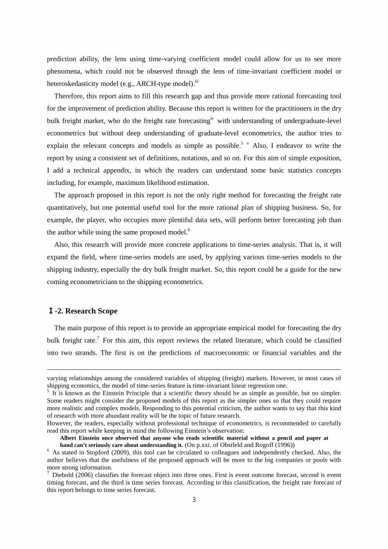
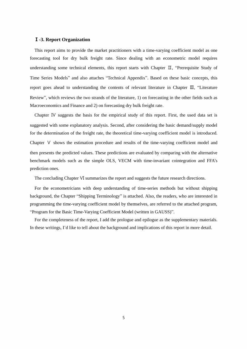
Consider the following figure of freight rate data in the dry bulk Capesize market.

Figure Ⅱ-1. Capesize Freight Rate (monthly average of 4TC daily averages, Baltic Exchange)

Source: Clarkson

For example, the freight rate in Sep. 2005 is 42,675$/day, in May 2008 201,136$/day, in Nov. 2008

is 3,995$/day, and in Dec. 2011 30,651$/day. In every period, we can think that the observation is

yielded by the related random variable, Yt.9 That is, the observed time series data can be thought as a

particular realization of a stochastic process, {Y1,⋯ , YT}. For these relevant concepts, a brief

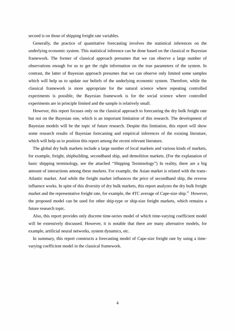
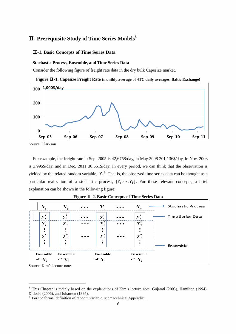
explanation can be shown in the following figure:

Figure Ⅱ-2. Basic Concepts of Time Series Data

Source: Kim’s lecture note

8 This Chapter is mainly based on the explanations of Kim’s lecture note, Gujarati (2003), Hamilton (1994),

Diebold (2006), and Johansen (1995). 9 For the formal definition of random variable, see “Technical Appendix”.

0

100

200

300

Sep-05 Sep-06 Sep-07 Sep-08 Sep-09 Sep-10 Sep-11

1,000$/day

7

In words, a stochastic process is a sequence of random (stochastic) variables ordered in time.

Ensemble is a collection of all possible realizations of a stochastic process. Time series data is a

particular realization of a stochastic process. In typical situation, we have only a particular time series

data, {y11, y2

1,⋯ , yt1, ⋯ , yT

1}. In contrast with cross-sectional data, usually we cannot expand the data

set by repeating the relevant experiments or by surveying more samples.10

Stationarity and Ergodicity

Only using time series data, we should impose some assumptions on the stochastic process in order

to derive information from the time series data. For example, consider the following data, which are

the change rate of the above freight rates:

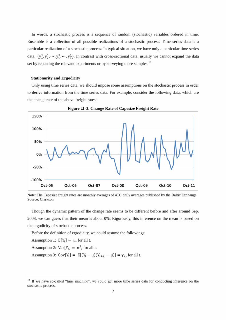
Figure Ⅱ-3. Change Rate of Capesize Freight Rate

Note: The Capesize freight rates are monthly averages of 4TC daily averages published by the Baltic Exchange

Source: Clarkson

Though the dynamic pattern of the change rate seems to be different before and after around Sep.

2008, we can guess that their mean is about 0%. Rigorously, this inference on the mean is based on

the ergodicity of stochastic process.

Before the definition of ergodicity, we could assume the followings:

Assumption 1: E[Yt] = μ, for all t.

Assumption 2: Var[Yt] = σ2, for all t.

Assumption 3: Cov[Yt] = E[(Yt − μ)(Yt+k − μ)] = γk, for all t.

10

If we have so-called “time machine”, we could get more time series data for conducting inference on the

stochastic process.

-100%

-50%

0%

50%

100%

150%

Oct-05 Oct-06 Oct-07 Oct-08 Oct-09 Oct-10 Oct-11

8

If the above three assumptions hold, then the process for Yt is said to be covariance-stationary or

weakly stationary. Broadly speaking, a stochastic process is said to be stationary if its mean and

variance are constant over time and the value of the covariance between the two time periods depends

only on the distance or gap or lag between the two time periods and not the actual time at which the

covariance is computed.

In order to define the ergodicity, let’s define the time average of the time series as follows:

y̅ ≡ (1 T⁄ )∑ yt1T

t=1 . --- (Ⅱ-1)

A covariance-stationary process is said to be ergodic for the mean if (Ⅱ-1) converges in probability

to E[Yt] as T → ∞.11

For example, the below AR(1) and MA(1) are both covariance-stationary and

ergodic for the mean.12

Therefore, as shown in Figure Ⅱ-3, we could conclude that the average of change rate is about 0%,

given that the underlying process is ergodic for the mean and the sample size is sufficiently large.

Ⅱ-2. Univariate Case: AR, MA, Wold’s Decomposition, Impulse-Response Analysis,

and Unit Root13

Autoregressive (AR) Process

Consider the following first-order autoregressive (AR(1)) process:

yt = c + ∅ × yt−1 + εt, --- (Ⅱ-2)

where |∅| < 1, and {ϵt} is a white noise in the sense that E[εt] = 0, E[εt2] = σ2, and

E[εtετ] = 0 for t ≠ τ.14

It can be proven that, when |∅| < 1, the above AR(1) process is covariance-stationary and ergodic

for the mean.

11

This means that, if the sample size is sufficiently large, the time average becomes equal to the ensemble mean,

μ. 12

It is notable that the ergodicity is a sufficient condition for the covariance-stationarity but the covariance-

stationarity is not the sufficient condition for the ergodicity. So, the covariance-stationarity is a necessary

condition for the ergodicity. 13

After studying this section, for more understanding the related econometric concepts such as ARIMA and

Box-Jenkins methodology, see “Technical Appendix”. 14

For the notational simplicity, in this report, without a particular note, εt is assumed to be a white noise with

normal distribution is denoted by “~iidN(0, σ2)”, which is read “independently and identically distributed with

normal distribution, its mean is 0 and its variance is σ2”.

9

However, a generalized pth-order autoregression, denoted AR(p), is as follows:

yt = c + ∅1 × yt−1 + ⋯+ ∅p × yt−p + εt. --- (Ⅱ-3)

Moving Average (MA) Process

Consider the following first-order moving average (MA(1)) process:

yt = μ + εt + θ × εt−1. --- (Ⅱ-4)

It can also be proven that, regardless of the value of θ, the above MA(1) process is covariance-

stationary. Furthermore, if {ϵt} is Gaussian white noise, which means {ϵt} is a sequence of

independent random variables each of which has a N(0, σ2) distribution, then the MA(1) is ergodic

for all moments.15

Wold’s Decomposition Theorem and Impulse-Response Analysis

Wold’s decomposition theorem says that all of the covariance-stationary process can be written in

the following form:

yt = μ + ∑ ψj × εt−j∞j=0 , --- (Ⅱ-5)

where ∑ ψj2∞

j=0 < ∞ with ψ0 = 1.

Based on this excellent property of covariance-stationarity, we can analyse the impulse-response

mechanism. For example, how much will Yt+j change by the unit shock, εt? This response of Yt+j

from the impulse εt is measured as ψj, based on the following reason:

∂yt+j

∂εt=

∂yt

∂εt−j= ψj.

Unit Root Stochastic Process

Up to now, we discuss the properties of stationary process. However, in reality, many time series

data seem to be nonstationary, which simply means “not stationary” in the sense just defined above. In

other words, a nonstationary time series will have a time-varying mean or a time-varying variance or

both.

A well-known nonstationary stochastic process is the random walk model.16

Random walk without

15

Without introducing the rigorous definitions of all moments, simply speaking, the first moment is the mean

and the second moment is variance. Similarly, higher moments can be defined. 16

The term random walk is often compared with a drunkard’s walk. Leaving a bar, the drunkard moves a

random distance εt at time t, and, continuing to walk indefinitely, will eventually drift farther and farther away

10

drift has the following form:

yt = yt−1 + εt. --- (Ⅱ-6)

In contrast, random walk with drift17

has the following form:

yt = μ + yt−1 + εt. --- (Ⅱ-7)

This random walk process is a typical unit root18

stochastic process. We also call the random walk

model as “integrated of order 1, denoted as I(1)”.19

Similarly, if a stochastic process has to be

differenced twice to make it stationary, we call it as “integrated of order 2”. In general, if a stochastic

process has to be differenced d times to make it stationary, that time series is said to be “integrated of

order d”. A stochastic process yt integrated of order d is denoted as yt ~ I(d).

With regard to the random walk with drift, we should distinguish the “difference stationary process

(DSP)” from the “detrend stationary process (TSP)”. We can write (Ⅱ-7) as the following:

yt − yt−1 = ∆yt = μ + εt. --- (Ⅱ-8)

It means that yt will exhibit a positive (μ > 0) or negative (μ < 0) trend. Such a trend is called a

stochastic trend. Equation (Ⅱ-8) is a DSP because the nonstationarity in yt can be eliminated by

taking first difference of the process.

In contrast, consider the following deterministic trend model:

yt = β1 + β2 × t + εt. --- (Ⅱ-9)

It is called as a TSP (deTrend Stationary Process). Though the mean of yt is β1 + β2 × t, which

is not constant, its variance is constant as E[εt2]. It is notable that, once the values of β1 and β2 are

known, the mean can be forecast perfectly. Therefore, if we subtract the mean of yt from yt, the

resulting process will be stationary, hence the name is detrend stationary.

from the bar. The same is said to about stock prices. Today’s stock price is equal to yesterday’s stock price plus a

random shock. (On p.798. of Gujarati (2003)) 17

In the equation (Ⅱ-7), μ is known as the drift parameter. 18

From yt = yt−1 + εt, we get yt − yt−1 = (1 − L)yt = εt, where L is the lag operator. The term unit root

refers to the root of the polynomial in the lag operator: If you set (1-L) = 0, we obtain L = 1, hence the name is

unit root. (On p.802. of Gujarati (2003)) 19

The expression, “integration” comes by the analogy with calculus. As we can undo an integral by taking a

derivative, we say that a nonstationary series is integrated if its nonstationarity is appropriately undone by

differencing. (On p.289. of Diebold (2006))

11

Ⅱ-3. Multivariate Case: VAR, VECM, and Co-integration

Consider the following 2-dimensional second-order autoregressive process (x1t x2t)′:

x1t = π11,1 × x1,t−1 + π12,1 × x2,t−1 + π11,2 × x1,t−2 + π12,2 × x2,t−2 + c1 + ε1t , --- (Ⅱ-10)

x2t = π21,1 × x1,t−1 + π22,1 × x2,t−1 + π21,2 × x1,t−2 + π22,2 × x2,t−2 + c2 + ε2t . --- (Ⅱ-11)

These two individual equations can be expressed in the following matrix form:

xt = Π1xt−1 + Π2xt−2 + C + εt , --- (Ⅱ-12)

where xt = [x1t

x2t], Πp = [

π11,p π12,p

π21,p π22,p] with p = 1 or 2, C= [

c1

c2], and εt = [

ε1t

ε2t].

This equation is called a vector autoregressive (VAR) model. It can also be generalized to the

VAR(p) model.20

From (Ⅱ-12), we can derive the following equation:

xt − xt−1 = (Π1 − I)xt−1 + Π2xt−2 + C + εt

= (Π1 + Π2 − I)xt−1 − Π2(xt−1 − xt−2) + C + εt

= Πxt−1 − Π2(xt−1 − xt−2) + C + εt, --- (Ⅱ-13)

where Π = Π1 + Π2 − I.

As implied by (Ⅱ-13), we can write VAR(p) in the following vector error correction model

(VECM):21

Δxt = Πxt−1 + ∑ ΓiΔxt−ip−1i=1 + C + εt , --- (Ⅱ-14)

where Π = ∑ Πipi=1 − I and Γi = −∑ Πj

pj=i+1 .

Up to now, we have not discussed the stationarity problem of VAR model. However, similar with

univariate case, there are many VAR processes which are nonstationary. For example, consider the

following stochastic processes:

x1t = μt + ε1t, --- (Ⅱ-15)

x2t = μt + ε2t, --- (Ⅱ-16)

20

The use of VAR model in macroeconomics is strongly advocated by Sims (1980). 21

Engle and Granger (1987) and Johansen (1988) deal with this VECM approach.

12

μt = μt−1 + ε3t. --- (Ⅱ-17)

Given the dynamics of the above vector (x1t x2t)′, it is not stationary. That is, because μt is the

random walk without drift, xit with i = 1, 2 is not stationary. However, as in the univariate case, the

first-difference of the vector is stationary. Furthermore, μt functions as a common stochastic trend in

the processes of x1t and x2t. Therefore, x1t and x2t could have a long-run relationship. Simply

speaking, the information on this long-run relationship is contained in the matrix Π of (Ⅱ-14). In

literature, the variables which has long-run relationship among them is said to be cointegrated.22

23

Assuming Π = αβ′24 transforms (Ⅱ-14) into the following:

Δxt = αβ′xt−1 + ∑ ΓiΔxt−ip−1i=1 + C + εt . --- (Ⅱ-18)

When xt is 2-dimensional, the first-line equation is expressed as follows:

Δx1t = α1 × (β1 × x1t−1 + β2 × x2t−1 ) + ∑ Γ1,ip−1i=1 Δxt−i + c1 + ε1t. --- (Ⅱ-19)

The vector (β1 β2) is said to be a cointegrating vector which represents the long-run relationship

between two variables. The parameter α1 governs the adjustment speed of Δx1t for the deviation

from the long-run equilibrium, (β1 × x1t−1 + β2 × x2t−1). However, (β1 β2) is not unique. That is,

for nonzero k, (kβ1 kβ2) can also be a cointegrating vector. Therefore, some normalization is

required.

For example, from the model consisting of the equations, (Ⅱ-15) ~ (Ⅱ-17), consider the following

process:

zt ≡ x1t − x2t = ε1t − ε2t. --- (Ⅱ-20)

In this case, the cointegrating vector representing the long-run relationship is (1 -1). The deviation

from the long-run equilibrium is zt.

In summary, given that xt ~ I(1), if there is long-run relationship among the variables, which can

be represented by the cointegrating vector β, then β′xt~ I(0).

22

According to Watson (1994), the I(1) cointegrated model is represented in the following four ways: 1) VECM

representation, 2) moving average representation, 3) common trends representation, and 4) triangular

representation. 23

Regarding the cointegration, the spurious problem should be understood. For this problem, see “Technical

Appendix”. 24

The condition for the existence of such αβ′ is suggested on p.49. of Johansen (1995).

13

Ⅲ. Literature Review

Ⅲ-1. Literature on Forecasting in Other Fields Including Macroeconomics and Finance

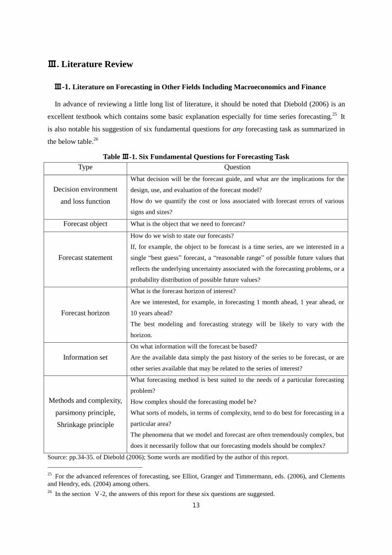
In advance of reviewing a little long list of literature, it should be noted that Diebold (2006) is an

excellent textbook which contains some basic explanation especially for time series forecasting.25

It

is also notable his suggestion of six fundamental questions for any forecasting task as summarized in

the below table.26

Table Ⅲ-1. Six Fundamental Questions for Forecasting Task

Type Question

Decision environment

and loss function

What decision will be the forecast guide, and what are the implications for the

design, use, and evaluation of the forecast model?

How do we quantify the cost or loss associated with forecast errors of various

signs and sizes?

Forecast object What is the object that we need to forecast?

Forecast statement

How do we wish to state our forecasts?

If, for example, the object to be forecast is a time series, are we interested in a

single “best guess” forecast, a “reasonable range” of possible future values that

reflects the underlying uncertainty associated with the forecasting problems, or a

probability distribution of possible future values?

Forecast horizon

What is the forecast horizon of interest?

Are we interested, for example, in forecasting 1 month ahead, 1 year ahead, or

10 years ahead?

The best modeling and forecasting strategy will be likely to vary with the

horizon.

Information set

On what information will the forecast be based?

Are the available data simply the past history of the series to be forecast, or are

other series available that may be related to the series of interest?

Methods and complexity,

parsimony principle,

Shrinkage principle

What forecasting method is best suited to the needs of a particular forecasting

problem?

How complex should the forecasting model be?

What sorts of models, in terms of complexity, tend to do best for forecasting in a

particular area?

The phenomena that we model and forecast are often tremendously complex, but

does it necessarily follow that our forecasting models should be complex?

Source: pp.34-35. of Diebold (2006); Some words are modified by the author of this report.

25

For the advanced references of forecasting, see Elliot, Granger and Timmermann, eds. (2006), and Clements

and Hendry, eds. (2004) among others. 26

In the section Ⅴ-2, the answers of this report for these six questions are suggested.

14

The papers reviewed in this section are all about 1) cointegration in VAR framework, 2) time-

variation of parameters, 3) Bayesian versus classical frameworks, 4) endogeneity problem, especially

correlation between the stochastic regressor and disturbance term, and 5) out-of-sample forecasting.

These issues are dealt with simultaneously in the individual paper. So, the sub-title leading to the

reviewed papers is only about the main topic, not the exclusive descriptive qualifier.

Cointegration in VAR framework

Stock and Watson (2001) show the usefulness of VAR model in forecasting macroeconomic

variables, while they argue that the VAR models have been proven to be powerful and reliable tools in

the jobs of data description and forecasting but have not been proven in the jobs of structural

inference and policy analysis.

De Mello (2009) argues that more structured VAR model could yield more accurate forecast of the

UK tourism expenditure shares for France, Spain and Portugal. Their following sentences are notable:

“When well specified, these models can provide not only a precise description of the data generating

process but also, and subsequently, accurate predictions for the values of the variable of interest. Thus,

the building of econometric models, even for the sole purpose of forecasting, must not disregard the

fundamental dimension of an appropriate formal specification. It is this dimension that allows

econometric models to provide reliable information for both explaining the past and predicting the

future”.27

Time-Variation of Parameters

Quintos and Phillips (1993) propose an approach to testing for coefficient stability in cointegrating

regressions of time series models. The considered test statistic is the one-sided version of the

Lagrange Multiplier (LM) test. Their null hypothesis is that there is cointegration. The basic notion is

that a test for the hypothesis that the long-run coefficient is constant can be interpreted as testing the

null hypothesis of cointegration. This notion leads to that, in the time-varying coefficient model, the

shock variance of the random work process for the coefficient dynamics should be zero under the null

hypothesis of cointegration. Though, as explained in Chapter Ⅱ, usually the cointegrating vector is

assumed to be constant, there is no a prior rationale for excluding the possibility of time variation of

cointegrating vector.28

Facing a lot of evidences for the absence of cointegration in economic variables, Park and Hahn

(1999) propose that there could be time-varying cointegration relationship. That is, there could be

27

This view point is almost the same for the structural models in the macroeconomic forecasting as explained

in Diebold (1998) or chapter 14 of Diebold and Rudebusch (1999). 28

This time variation in the cointegrating vector is the main property of the empirical model of this report.

15

parameter instability in the cointegration regressions. Their model is as follows:

yt = αt′ xt + εt, --- (Ⅲ-1)

αt = α(t

n), --- (Ⅲ-2)

where α is a smooth function defined on [0, 1] and n is the sample size.

They use the Fourier flexible form to approximate the smooth time-varying parameter

unparametrically. In order to illustrate the practical relevancy of their model, they consider the U.S.

automobile demand function. Using some test statistics, they argue that the cointegrated model with

time-varying coefficient is strongly supported by the data. In addition, they argue that, without

coefficient time variation, there could be mistakes as from the spurious regression problem.29

Zuo and Park (2011) apply the smooth time-varying cointegrating regression approach suggested

by Park and Hahn (1999) to the money demand analysis of China. They use the quarterly data from

1996Q1 through 2009Q1. Particularly, they show the properties of time-varying income, interest rate,

real stock price elasticities of money demand.

Similar to Park and Hahn (1999), Bierens and Martins (2010) consider the following time-varying

VECM representation:

Δxt = Πtxt−1 + ∑ ΓiΔxt−ip−1i=1 + εt . --- (Ⅲ-3)

Their objective is to test the null hypothesis of standard time-invariant cointegration with the

alternative hypothesis of time-varying cointegration. They approximate the dynamics of cointegration

time variation by using orthogonal Chebyshev time polynomials, which captures smooth time

transition of the cointegrating vectors. For estimation, they use MLE. As an empirical application,

they deal with the purchase power parity (PPP) theory.

Park and Kim (2009) apply the time-varying cointegration model to investigating the consequence

of the existence of firms which are not paying out dividends on the relationship between aggregate

dividends and stock price. In order to test the constant cointegration null hypothesis against the time

varying cointegration between the aggregate dividends and stock price, they employ the two test

methods. One is nonparametric which is suggested by Park and Hahn (1999). The other is parametric

which is suggested by Bierens and Martins (2010). Furthermore, for predicting stock returns,30

they

estimated a new predictor variable, which is stationary deviation from the time-varying cointegration

29

Spurious regression problem is that, when the relevant variables are I(1) and they are not related in fact, the

regression results could show that there seem to be statistically significant relationships. 30

Fama and Schwart (1977) is an early example of stock return prediction. In order to estimate the extent to

which various assets were hedges against the expected and unexpected components of the inflation rate during

the period 1953-1971, they use a kind of predictive regression model.

16

relationship between dividends and stock price.31

According to their analysis, this newly developed

variable has stable and strong ability to forecast stock returns from the out-of-sample analysis as well

as in-sample analysis.

Brown, Song and McGillivray (1997) consider the time-varying coefficient model with the

following form:32

yt = β1x1t + β2tx2t + εt, --- (Ⅲ-5)

β2t = β2t−1 + γzt + ω1t. --- (Ⅲ-6)

Regarding this time-varying coefficient model as a basic forecasting model, they also compare the

three different forecasting results of 1) recursive least square estimation, 2) cointegration approach

with constant parameter, and 3) VAR and AR estimation. In conclusion, they argue that the TVC

specification outperforms the alternative constant parameter specifications of UK house prices.

Bayesian versus Classical Frameworks

Sims (1993) applies the time-varying parameter model in the Bayesian framework to forecasting

macroeconomic variables. Particularly, it is evaluated so that it produces drastically better forecasts of

the price level variable than the previous Bayesian VAR model.

Using a Bayesian model averaging approach, Dangl and Halling (2011) apply predictive regression

model with the time-varying coefficients to financial data, for example, monthly S&P 500 index.

Especially, regarding the predictability problem, they conclude that there are statistical and economic

evidence of out-of-sample predictability: relative to an investor using the historic mean, an investor

using their methodology (a kind of Bayesian averaging approach with time-varying coefficients)

could have earned consistently positive utility gains (between 1.8% and 5.8% p.a. over different time

periods). They also argue that predictive models with constant coefficients are dominated by models

with time-varying coefficients. In this paper, it is notable that the poor performance of regime-

switching model for out-of-sample forecasting is due to the unreliable estimates of the timing of

breaks and of the size of the shift in real-time context.33

Also, they mention that the coefficient

variation can stem from the changes in market sentiment, which property is presumed to be the main

cause of the coefficient variation of this report. Finally, as in this report, they model the dynamics of

the coefficients as a random walk process.

31

When deriving this deviation, they use the time-varying cointegration regression approach of Park and Hahn

(1999). 32

The variable zt of (Ⅲ-6) is called as “driver variable”. 33

This point is originally suggested in Lettau and S. Van Nieuwerburgh (2008).

17

Koop, Leon-Gonzalez and Strachan (2011) point out that both economic theory and empirical

reality need a time-varying parameter vector error correction model (TVP-VECM) comparable to the

TVP-VAR.34

However, while there are a large number of theoretical and empirical papers that model

the nonlinearity in cointegrating relationship, as they argue, this effort is non-Bayesian with few

exceptions. So, they aim to develop Bayesian methods for TVP-VECM.

Particularly, they consider the following kind of TVP-VECM:

Δxt = αtβt′xt−1 + ∑ Γi,tΔxt−i

p−1i=1 + ct + εt , --- (Ⅲ-4)

where εt are independent N(0, Ωt).

However, the time-varying cointegrating space is modeled as similar to stationary AR(1) process by

using the methods from the directional statistics literature. They point out that this kind of stationarity

condition of the cointegrating space is necessary to ensure the property that “the cointegration space

today has a distribution that is centered over last period’s cointegrating space”.35

They also note the

problem that, if the cointegrating space is a random walk process, the cointegrating vector would

wander far from the origin.36

However, in their specification, the expected value of cointegrating

space at time t equals the cointegrating space at time t-1.

Regarding the notion of cointegration, their following remark is notable:

We note that cointegration is typically thought of as a long-run property, which might suggest a

permanence which is not relevant when the cointegrating space is changing in every period.

Time-varying cointegration relationships are better thought of as equilibria toward which the

variables are attracted at any particular point in time but not necessarily at all points in time.

These relations are slowly changing. (On p.212. of Ibid.)

As an empirical application, they consider the Fisher effect by using UK quarterly data. Importantly,

they argue that, instead of finding support for or against an economic hypothesis, we can conclude

that it (economic theory, i.e., Fisher effect hypothesis) holds at some points in time, but not others.

Also, they show that allowing for time-variation only in the cointegrating space and error covariance

matrix yields the best empirical model.

34

In their paper, as usually done in TVP-VAR, all the coefficients of VECM except the cointegration

coefficients are assumed to follow the random walk if they are time-varying. 35

It is notable that this property is desired in specifying random walk evolution for VAR parameters of TVP-

VAR molel. 36

This problem is applied to the model of this report. Since this report does not develop an econometric theory

on the suggested time-varying cointegration coefficients with random walk dynamics, the associated statistical

properties should be analysed for more rigorous inference. So, this econometric development will be an

important future research topic.

18

When forecasting as in this report, we presumably think that the true conditional expected value of

dependent variable is equal to the regression-based conditional mean. This is true if the predictor

variables are perfect in the sense that the equality should hold. However, in reality, there seem to be a

large number of cases where the equality does not hold. Facing with this problem, Pastor and

Stambaugh (2009) propose a Bayesian solution, which is called as “predictive system” compared to

the usual “predictive regression”.37

They argue that their proposed Bayesian “predictive system”

approach allows us to conduct clean finite-sample inference about various properties of the expected

value.

In the case in which the endogenous variables are given as the point values or some interval for

conditional forecasting, there had been no method of computing the exact finite sample distribution of

conditional forecast. Waggoner and Zha (1999) provide a solution to this problem by using Bayesian

methods. Also, this paper considers the issue of parameter uncertainty. In order to derive the finite-

sample distribution of conditional forecasts, they use two algorithms. One is for the hard conditions,

where the future values of variables are fixed at some points. The other is for the soft conditions,

where the future values of variables are restrained over some interval.38

Endogeneity Problem (Correlation between the Stochastic Regressor and Disturbance Term)

Stambaugh (1999) deals with a kind of endogeneity problem in predictive regression method.

Particularly, when there is correlation between the stochastic regressor and the disturbance term, it

shows that the p-value with conventional significance level, e.g., 5%, under the classical framework

would makes us to accept a null hypothesis but the posterior distribution under the Bayesian

framework has lower probability that the null hypothesis holds than 5%. That is, this paper attempts to

show the differential properties of classical and Bayesian approaches.

Similar to the motivation of Stambaugh (1999), Kim (2006) considers the endogeneity problem in

the case in which there exists correlation between the stochastic regressor and the disturbance term.

However, the model considered in Kim (2006) is the time-varying parameter model. In order to

appropriately handle the endogeneity problem, he derives a Heckman-type two-step approach.39

Also,

the conventional Kalman filter is applied to the regression equation by implementing appropriate bias

correction terms obtained from the first-step regression. With this proposed two-step approach, we can

obtain consistent estimates of the hyper-parameters of the model and the conventional Kalman filter

37

In this terminology, when the predictors approach perfection, the system-based conditional expected value

approaches the regression-based conditional mean. 38

Since the sample of this report is relatively small, this method, which provides the exact finite-sample

distribution of conditional forecasts for time-varying parameter multivariate model (e.g., VAR) by using

Bayesian approach, will be very helpful for the improvement of the forecasting task which uses the model of

cointegration regression with time-varying coefficients. However, this topic remains as a future research subject. 39

Heckman (1976).

19

provides us with correct inferences on the time-varying coefficients.

Kim and Nelson (2006) apply this Heckman-type two-step approach to investigating the history of

the U.S. Fed’s conduct of monetary policy. As a result, contrast with the conventional division of the

sample into Pre-Volcker and Volcker-Greenspan periods, they divide the history since the early 1970s

into the 1970s, the 1980s, and the 1990s.

Out-of-Sample Forecasting

In this report, the forecasting performance is evaluated under the so-called out-of-sample context.

Regarding this out-of-sample exercise, Hjalmarsson (2006) provides important information by using a

simple Monte Carlo experiment. According to its argument, similar out-of-sample results to those of

Goyal and Welch (i.e., no predictive gains of virtually all variables that have been proposed as

predictors of future stock returns)40

are found even when the postulated forecasting model is in fact

the true data generating process. This is thought of as due to the fact that any predictive component in

stock returns must be small, if it does exist. So, in order to accurately estimate a very small coefficient,

large amounts of data are needed. That is, when testing for stock return predictability, the sample sizes

in most relevant cases are too small relative to the size of the slope coefficient for any predictive

ability to show up in out-of-sample exercises. In summary, it argues that we should not disregard the

econometric in-sample results in favor of out-of-sample results.

Ibrahim and Florkowski (2007) compare the out-of-sample forecast performances among 1)

univariate ARIMA, Engle-Granger two-step,41

Johansen’s models42

by using the monthly U.S. time

series data set for the period from 1991 to 2004. According to their results, ARIMA models seem to be

useful for short-term forecasts, but for longer-term forecasts the cointegration technique seems to be

useful.

40

Goyal and Welch (2003) and Goyal and Welch (2004). 41

Engle and Granger (1987). 42

Johansen (1998).

20

Ⅲ-2. Literature on Forecasting Dry Bulk Freight Rate43

Alizadeh and Nomikos (2010) provide a comprehensive review on the subject of structure, dynamic

properties, and the relationships in the dry bulk sub-markets which can be classified by size into Cape,

Panamax, and Hany-class markets and by relevant activity into freight markets (spot versus time-

charter markets), newbuilding, secondhand ship, and demolition markets.

Using Forward or Futures Variables44

Alizadeh and Nomikos (2003) show that market participants can get more accurate forecasts of

freight rates by using FFAs rather than BIFFEX (Baltic International Freight Futures Exchange for

trading freight futures contracts with settlement based on the Baltic Freight Index) contracts, in which

they consider the 2 Panamax routes and 2 Capesize routes.

Similar with Kavussanos and Nomikos (2003),45

Batchelor, Alizadeh and Visvikis (2007) apply

various time series models of ARIMA, VAR, VECM, S-VECM (Seemingly unrelated regression

equations VECM) to investigating the relationship between the Panamax spot rates and FFA rates and

then forecasting these variables. The considered routes are Panamax Atlantic routes 1 and 1A whose

daily sample is 16. Jan. 1997 to 31 July 2000, and Panamax Pacific routes 2 and 2A whose sample

period is 16. Jan. 1997 to 30 April 2001.46

47

They take the hypothesis that, if the forward market is liquid enough to embody some information

about futures spot rates into the forward prices, we should observe cointegration between them, and

convergence of spot towards forward rates, rather than vice versa. Indeed, according to their test

results for the cointegration relationship, the spot and FFA prices are cointegrated in all routes. Also,

across all routes the adj-R2 for changes in spot rates are higher than those of forward rates, indicating

potentially higher predictability in spot rates than forward rates.48

But in the respect of adjustment

43

Even though a large number of researchers try to insist that their (empirical) findings could apply to the

course of future events, the fact that their results should be based on the past events, not on the future ones,

could imply limitation of their usefulness for the forecasting purpose. This aspect would require that we should

cautiously review the literature focusing on the data set. 44

Regarding FFA, there are some interesting researches. Using the so-called GJR-GARCH model (suggested in

Glosten, Jagannathan and Runkle (1993)), Kavussanos, Visvikis, and Batchelor (2004) examine the impact of

FFA trading on spot market price volatility in Panamax market. Using VECM-GARCH model, Kavussanos and

Visvikis (2004) investigate the lead-lag relationship in daily returns and volatilities in Panamax market. 45

In contrast, Kavussanos and Nomikos (2003) deal with BIFFEX rates. 46

The former sample is ended earlier than the latter one because, after 31 July 2000, the FFA brokers stopped

publishing the relevant FFA quotes, which is the data source. 47

The data sources are as follows: For spot rate, it is the Baltic Exchange and for FFA rate it is collected

manually from the records of Clarkson’s Securities Ltd. 48

The highest adj-R2 is 0.5892 for spot rate and 0.0715 for FFA rate, respectively. This relatively low adj-R2

could imply there is some omitted variables in the regression equations. So, regression equations with more

variables are required so that, first, the resulting adj-R2 will increase and thus our perception of the relevant

shipping markets will be improved.

21

speed, contrary to their expectation, forward rates adjust more strongly than spot rates in three of the

four routes.49

However, out-of-sample forecasting with the VECM models shows that they are not

helpful in predicting forward rate behavior, but do help predict spot rates, which is more consistent

with market efficiency.50

Alizadeh, Adland and Koekebakker (2007) examine whether the 6-month implied forward time

charter (IFTC) rate is an unbiased predictor of future TC rates. The data set is weekly and its sample

period is 1 Jan. 1989 to 27 June 2003. The considered ship sizes are 1) Capesize (127,000 DWT), 2)

Panamax (65,000 DWT), 3) Handymax (40,000 DWT).51

The IFTC is calculated in the following way: At time t, there are two separate TC rates, i.e., 6-

month and 12-month TC rates. Based on the present value model and efficient market hypothesis

(EMH), the expectation of 6-months ahead 6-month TC rate can be calculated, which is the same as

the IFTC.

As one of the tests of unbiasedness, the cointegraion approach requires that the IFTC at 6-month

early time and present TC should be cointegrated. According to their test results, we cannot reject the

cointegration relationship at any significance level.

However, apart from the unbiasedness, EMH could imply that IFTC should provide “the most

accurate forecast for the future values of TC rates amongst all competing forecast methods”. With

regard to this predictability, there are some contradicting empirical results. First, Based on RMSE

metric and Theil’s U statistic,52

the comparisons of the forecasting performance with those of ARIMA,

VAR, and VECM models show that IFTC provides the most accurate forecast, which is in line with

the notion of the EMH in freight rate formation. But, based on the simple chartering strategy, MA

strategy, there has been economically significant excess profit. Although this fact could imply that

there has been a time-varying risk premium, it also implies that there has been “predictable mispricing

of the implied forward freight rate”. This would imply that the market is inefficient. So, we could

conclude that the validity of the unbiasedness hypothesis, in the context of the term structure of

freight rates, is a necessary but not sufficient condition for the EMH to hold.

Additionally their following result is notable: The market forecasts a future 6-month TC rate that is

too low during upturns in the freight market. This bias implies that, based on the unbiasedness, the

market must forecast a future 6-month TC rate that is too high during market downturns.

49

In this regard, they note the dangers of forecasting with VECM when the underlying market is evolving and

the parameter estimates conflict with sensible theoretical priors. This caution about the evolution of market is

reflected in this report in the sense that the time-variation of parameters could incorporate the information on the

market evolution. 50

In contrast to Kavussanos and Nomikos (2003) with overlapping forecast intervals, Batchelor, Alizadeh and

Visvikis (2007) use the “independent out-of-sample N-period ahead forecasts” as suggested in Tashman (2000). 51

The data source is Clarkson’s Shipping Intelligence Network (SIN). 52

These two formulas are popular tools used for the evaluation of forecasting model. For example, for RMSE

(root mean squared error) metric see p.261 of Diebold (2006) and for Theil’s U statistic see p.324 of Ibid.

22

Kavussanos, Visvikis and Menachof (2004) consider the unbiasedness in the freight forward market.

In their introduction, there are two notable remarks, one is about the nature of forward freight market

and the second is about the purpose of investigating the unbiasedness hypothesis.

First, they explain the nature of forward freight market as follows: “The non-storable nature of FFA

market implies that spot and FFA prices are not linked by a cost-of-carry (storage) relationship, as in

financial and agricultural derivatives markets. Another feature of this derivative OTC market is the

asymmetric transaction costs between spot and FFA markets. These costs are higher in the spot freight

market (in relation to the FFA market), as it is the case for commodity spot versus futures market”.

Second, the purposes of investigating the unbiasedness hypothesis are as follows:

First, the underlying asset is a service. Second, the price discovery function provides a strong

and simple theory of the determination of spot prices that may prevail in the future. Third, if

forward prices fulfill their price discovery role, they provide accurate forecasts of the realized

spot prices, and consequently provide new information in the market and in allocating economic

resources (Stein (1981)). Decisions in the physical market are thus facilitated and can help

secure market agents’ cash-flow (transportation costs). … However, it must be noted that

market agents can initiate trade for several motives, such as heterogeneous expectations or

heterogeneous income/cost structures (Calvet, Gonzalez-Eiras and Sodini (2004)). Finally, the

apparent lack of research in the freight forward trades further motivates this investigation as

this is the only derivative instrument available to agents in the bulk shipping industry for

hedging purposes. Evidnece on whether agents in the shipping industry can use FFAs of

different maturities and for different routes, as unbiased predictors of spot freight rates, is very

important and provides a free source of information for decision-making. (On pp.243-244. of

Ibid.)

Their data set are monthly FFA and spot rates. The sample period is 1996:01 to 2000:12. The

considered routes are Panamax 1, 1A, 2, and 2A. For FFA variable, the average (mid-point) of bid and

offer quotes is used.53

FFA rate is from Clarkson Securities and spot rate is from Datastream.

The unbiasedness hypothesis is examined by testing the restrictions β1 = 0 and β2 = 1 in the

cointegration relationship β′xt = (1 β1 β2)(st−1 1 Ft−1,t−n−1′) where S is spot rate, F is FFA rate

and n is considered maturity. If these restrictions hold, then the price of the FFA contract is an

unbiased predictor of the realized spot price. According to their results, for the one- and two-months

53

We can get the Baltic assessment of FFA rates since Aug. 2005. This assessment data set could function as the

“best” daily price for forward (or futures) prices of dry bulk freight rate. However, when there has not existed

this data set, Kavussanos, Visvikis and Menachof (2004) say that, owing to the absence of this reliable data set,

it is more difficult to investigate whether derivatives prices informationally lead spot prices in the shipping

market than in organized futures exchanges. (See p.243. of Ibid.)

23

FFA prices, and for route 2 and 2A three-months FFA prices, the unbaiasedness hypothesis cannot be

rejected at conventional levels of significance. So, for the investigated routes and maturities for which

the unbiasedness holds, market agents can use the FFA prices as indicators of the future course of spot

prices in order to guide their physical market decisions.

Regarding the error correction coefficient (adjustment speed), both spot and FFA prices respond to

the long-run equilibrium in the one-month maturity, while in the two- and three-months maturities

only FFA prices respond to the previous period’s deviations from the long-run equilibrium

relationship. This finding is consistent with the hypothesis that past forecast errors affect the current

forecasts of the realized spot prices, i.e., FFA prices, but not the spot prices themselves.

Similar to Batchelor, Alizadeh and Visvikis (2007), Kavussanos and Nomikos (2003) apply various

time series models of ARIMA, VAR, VECM and random-walk models to investigating the

relationship between the Panamax spot rates and futures (BIFFEX)54

rates and then forecasting these

variables. The considered main issue is that, due to the non-storable nature of the shipping market,

spot and futures prices would not linked by a cost-of-carry relationship, and hence futures prices may

not contribute to the discovery of new information to the same extent as the markets for storable

commodities.55

For tackling this issue, they use the daily data set. Their sample period is 1 Aug. 1988 to 30 April

1998. The spot rates are from LIFFE (London International Financial Futures Exchange) and futures

are from Knight Ridder, Financial Times, and LIFFE.

Their major findings can be summarized as follows:

First, spot and futures prices stand in a long-run relationship between them.: hence, a VECM

can be used to investigate the short-run dynamics and the price movements in the two markets.

Second, causality tests and impulse response analysis indicate that futures prices tend to

discover new information more rapidly than spot prices. This pattern is thought to reflect the

fundamentals of the underlying asset since, due to the limitations of short-selling the underlying

spot index, investors who have collected and analysed new information would prefer to trade in

the futures rather than in the spot market. Third, information from the futures prices can be

used to generate more accurate forecasts of the spot prices but not the other way round. This

reflects that causality from futures to spot runs stronger than the other way and that most of the

variability in the futures returns is attributed to pure innovations which cannot be predicted.

54

In contrast, Batchelor, Alizadeh and Visvikis (2007) deal with FFA rates. 55

As Garbade and Silber (1983) is suggested as a reference, Kavussanos and Nomikos (2003) note that the

primary benefits of futures markets to economic agents are price discovery and risk management through

hedging. Price discovery is the process of revealing information about the future spot prices through the futures

markets. Risk management refers to hedgers using futures contracts to control their spot price risk. The dual

roles of price discovery and risk transfer provide benefits that cannot be offered in the spot market alone and are

often presented as the justification for futures tradeing. (On. p.203. of Ibid.)

24

Finally, the price discovery role of futures prices has strengthened in the period after the

exclusion of the handysize routes from the BFI: this is thought to be the result of the more

homogeneous composition of the index for this period. Overall, despite the non-storable nature

of the market and the thin trading, futures prices contribute to the discovery of new information

in the spot market, as in the case of other commodity and financial futures market. (On p.225. of

Ibid.)

Given that the above literature which shows that the futures, forward or implied freight rates could

inform the market participants of the course of future rates, the naturally resulting question will be

“Even though we can anticipate the future course of the spot rates with the futures, forward or implied

freight rates, at first without themselves, how can we predict the spot rates or themselves?”56

Freight Rate Determination Mechanism Model

Rim, Kim and Ko (2010) analyse the dynamic interrelationship among the demand, supply and

freight rate variables in the dry bulk market. For the empirical tool, they use a recursive VAR model.

The data set includes BDI, cargo volume and fleet capacity, which are similar to that of this report

except that this report adds the FFA assessment variable. While they don’t tackle the problem of

forecasting, their VAR model could be used as a forecasting tool.

The consecutive papers of Chung and Ha (2010b) and Chung and Ha (2010a) should be noted. Both

of them consider the China’s iron import, 3-month Eurodollar interest rate, and U.S. industry stock

price index as the explanatory variables for BDI. The first variable reflects a direct shipping demand

of China, the second is a proxy for the international financial condition which can influence the global

macroeconomic cycles, and the third shows whether U.S. economy is in the phase in boom or

recession. Particularly, Chung and Ha (2010b) show that there has been a cointegration relationship

between the BDI and the aforementioned explanatory variables by using the Pesaran’s cointegration

method and Chung and Ha (2010a) investigate the structural changes in the relationship between the

same variables by using the Kalman filter.

Importantly, the model structure of Chung and Ha (2010a) is the same as that of this report in that

both of them consider the time-varying coefficient model for the determination mechanism of dry

bulk freight rate. However, they differ substantially in the use of explanatory variables and thus the

relevant theory for the underlying economic shipping market. Moreover, this report considers both of

the freight rate determination mechanism and its forecasting performance, while Chung and Ha

(2010a) considers only the former theme, i.e., the freight rate determination.

56

This question shows the reason why this report considers the demand/supply model.

25

Forecasting Using VAR Model

Veenstra and Franses (1997) apply a VEC model to forecasting the freight rates of Capesize and

Panamax ships. They argue that the fact that the specification of the long-term relationship defined in

the VEC model does not improve the accuracy of short- or long-term forecasts can be interpreted as a

corroboration of the efficient market hypothesis.

Alternative Freight Rate Forecasting Methods Including Non-Linear Models

There have been some efforts to forecast dry bulk freight rate by using alternative methods to linear

regression approach.

Chang, Hsieh and Lin (2012) propose a non-linear regression model for the prediction of Capesize

dry bulk freight rate by using monthly data set of Clarkson. They use the exponential function for

finding the relationship between the market variables and time period, which is their nonlinearity. By

treating the secondhand ship prices as explanatory variable after some selection procedures, they

show the extent of prediction accuracy based on in terms of MAPE (Mean Absolute Percentage Error).

However, they don’t consider the nonlinearity in the relationship between the freight rate and

explanatory variables.57

Zhongzhen, Lianjie and Minghua (2011) apply the wavelet transform and support vector machine

combined model to forecasting BPI (Baltic Panamax Index) using the monthly average of BPI from

Jan. 2001 to May 2009. They insist that the proposed model has a very high goodness of fitness,

particularly in the peak and trough.

Veenstra and van Dalen (2011) suggest an interesting conjecture that brokers’ estimates58

add

something to a time series and this guesstimate may reflect the term structure model which exists in

the minds of the brokers, but perhaps not in practice. For this argument, they construct the weighted

unit value indices and duration indices59

solely based on actual fixtures which have been obtained

from Maritime Research Inc. (MRI) in the U.S.A. Furthermore, they argue that their duration indices

contain more information than the unit value indices or brokers’ estimates such as those of the Baltic

Exchange and Clarkson.

Similarly, while pointing out that many of popular freight rate time series do not reflect cost of use

or average charter levels in the market of new and existing contracts, Gratsos, Thanopoulou and

Veenstra (2012) show the stable relationship between contract duration and freight level. They argue

57

Their sample period is from Nov. 1995 to Sep. 2008, which excludes the period after 2008 global financial

crisis. Since they cannot consider the parameter change from the collapse of dry bulk markets of the crisis, their

nonlinearity model could not explain this post-crisis phenomenon. 58

When, for a specific commodity or route, there are no actual contracts reported, the Baltic Exchange indices

or Clarkson’s indices are completed based on brokers’ estimates. 59

The basic rationale for the duration indices is that the freight rates of both the newly concluded contracts and

the running fixtures are part of the economic reality and should therefore be included in the index construction.

26

that, while the shipper wishes to control the transport cost over a long period of time and/or encourage

the construction of bigger ships by using long-term period charters, the shipowners disagree that the

freight rates remain at low levels at a time of ample supply of tonnage like 1998 to 2003 owing to

long-term contract. This kind of argument is interpreted as suggesting that the incorporation of

contract duration is necessary for the improvement in accessing and forecasting the dry bulk freight

rate.

It is notable that Goulielmos and Psifia (2009) suggest an alternative approach to forecasting

weekly freight rates for one-year time charter 65,000 DWT bulk carrier. As analytical tools, they use

Rescaled Range Analysis, the related Hurst Exponent, Power Spectrum Analysis, V-statistic and BDS

Statistic. By nature, these tools are non-linear. They argue that this kind of non-linear analysis is

superior in forecasting vis-à-vis GARCH.

Although the analyzed market is the tanker one, there have been some efforts using Artificial

Neural Networks (hereafter ANN). First, Li and Parsons (1997) apply the ANN model to the tanker

market based on the monthly data set consisting of dirty tanker spot rate, tanker demand and the

tanker supply from January 1980 to October 1995. Second, Lyridis, Zacharioudakis, Mitrou, Mylonas

(2004) also apply the ANN model to the tanker market based on the monthly sample from October

1979 to December 2003. This ANN model is considered as a powerful tool for complex time series

data set because it can reflect the unstable relationships among the independent and dependent

variables.

Dikos, Marcus, Papadatos, Papakonstantinou (2006) apply a system-dynamics approach60

to tanker

freight modeling, While their method of system dynamics captures the essential features of several

shipping-industry situations, it also provides a powerful tool for evaluating managerial decisions and

what-if scenarios. Randers and Goluke (2007) also report the research efforts using the system

dynamics in tanker market. According to their results, the system dynamics succeeded in forecasting

turning points in the relevant shipping freight markets.

60

In comparison, Engelen, Dullaert, Vernimmen (2009) use a system dynamics method to assess the Efficient

Market Hypothesis (EMH) in the dry bulk shipping market.

27

Ⅳ. Data and Time-Varying Coefficient Model

Ⅳ-1. Data

Explanation of data set would be given after the introduction of the underlying economic model.

However, in the dry bulk shipping industry, the availability of data is somewhat limited partly because

there is no public entity with enforcement power which can collect the relevant information such as

the tonnage supply, seaborne transport demand, port congestion, lay-up ships, etc. These data are

gathered basically by the private organization. Therefore, the limitation of data set imposes the

constraint on the structure of the economic model for dry bulk freight market.61

As a result, the author

firstly introduces the data set used in this research.vii

This report aims to forecast the Cape-size dry bulk freight rate in so-called macro level.62

Usually,

the freight rate can be considered differently across the time span.63

For example, if the shipowner

expects that the future freight rate will increase, then he wants to fix a shorter-term contract (e.g.,

voyage or trip-charter contract). In the opposite case, he will try to fix a longer-term contract (e.g.,

Contract of Affreightment). However, this report deals with the freight rate, supply, demand and FFA

assessment at the monthly frequencies, hence this report is useful for the freight rate risk management

based on the monthly period.64

For example, many of the popular derivatives of dry freight rate based

on the Baltic Exchange indices are traded by using the settlement prices of the monthly average. In

addition, this time domain of this report is due to the fact that the supply/demand variables can be

observed on at least monthly basis.

61

This problem of data quality in the shipping market is not unique. The famous high-quality macro data, GDP,

is also related with this kind of data quality problem. Furthermore, from this problem, we cannot assess exactly

the performance of forecasting model. Stopford (2009) quotes the following sentence of M. Baranto: ‘The

analysis of forecasting errors is not a simple process – ironically it is as difficult as making forecasts’. This

means that care is needed to produce forecasts that are capable of being monitored quickly and easily by users.

(See p.741. of Ibid.) 62

In contrast, Alizadeh and Talley (2011) analyse the freight rate determination in micro level. So, it can be said

that the identification of the significant level of detail to work at is a very important issue. In theory more

information should lead to a more reliable result. However, the danger is that it is very time-consuming and can

easily generate so much detail that the underlying rationale of the forecast is lost. (p.720. of Stopford (2009)) 63

Regarding the various types of dry bulk freight contracts, see “Shipping Terminology”. 64

While reviewing the recent quantitative analyses, e.g., reduced form model, Glen (2006) points that fully

specified structural modeling for dry bulk freight market using monthly data may be an important research

agenda.

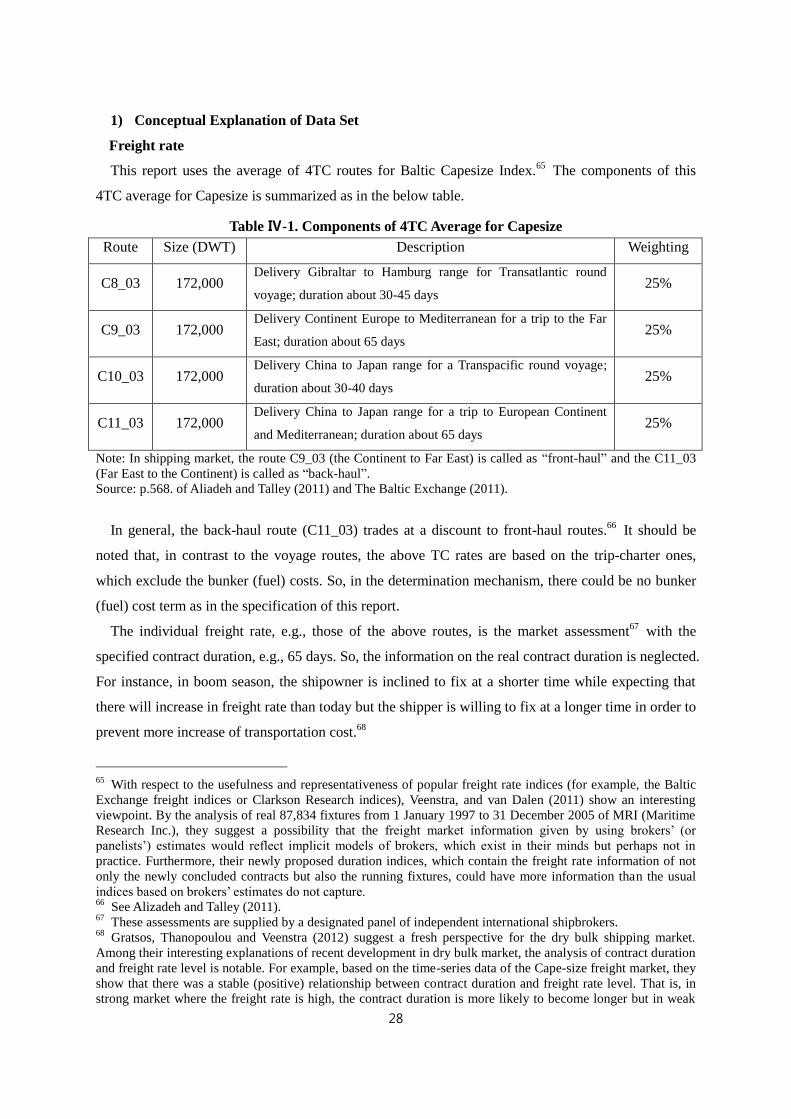
28

1) Conceptual Explanation of Data Set

Freight rate

This report uses the average of 4TC routes for Baltic Capesize Index.65

The components of this

4TC average for Capesize is summarized as in the below table.

Table Ⅳ-1. Components of 4TC Average for Capesize

Route Size (DWT) Description Weighting

C8_03 172,000 Delivery Gibraltar to Hamburg range for Transatlantic round

voyage; duration about 30-45 days 25%

C9_03 172,000 Delivery Continent Europe to Mediterranean for a trip to the Far

East; duration about 65 days 25%

C10_03 172,000 Delivery China to Japan range for a Transpacific round voyage;

duration about 30-40 days 25%

C11_03 172,000 Delivery China to Japan range for a trip to European Continent

and Mediterranean; duration about 65 days 25%

Note: In shipping market, the route C9_03 (the Continent to Far East) is called as “front-haul” and the C11_03

(Far East to the Continent) is called as “back-haul”.

Source: p.568. of Aliadeh and Talley (2011) and The Baltic Exchange (2011).

In general, the back-haul route (C11_03) trades at a discount to front-haul routes.66

It should be

noted that, in contrast to the voyage routes, the above TC rates are based on the trip-charter ones,

which exclude the bunker (fuel) costs. So, in the determination mechanism, there could be no bunker

(fuel) cost term as in the specification of this report.

The individual freight rate, e.g., those of the above routes, is the market assessment67

with the

specified contract duration, e.g., 65 days. So, the information on the real contract duration is neglected.

For instance, in boom season, the shipowner is inclined to fix at a shorter time while expecting that

there will increase in freight rate than today but the shipper is willing to fix at a longer time in order to

prevent more increase of transportation cost.68

65

With respect to the usefulness and representativeness of popular freight rate indices (for example, the Baltic

Exchange freight indices or Clarkson Research indices), Veenstra, and van Dalen (2011) show an interesting

viewpoint. By the analysis of real 87,834 fixtures from 1 January 1997 to 31 December 2005 of MRI (Maritime

Research Inc.), they suggest a possibility that the freight market information given by using brokers’ (or

panelists’) estimates would reflect implicit models of brokers, which exist in their minds but perhaps not in

practice. Furthermore, their newly proposed duration indices, which contain the freight rate information of not

only the newly concluded contracts but also the running fixtures, could have more information than the usual

indices based on brokers’ estimates do not capture. 66

See Alizadeh and Talley (2011). 67

These assessments are supplied by a designated panel of independent international shipbrokers. 68

Gratsos, Thanopoulou and Veenstra (2012) suggest a fresh perspective for the dry bulk shipping market.

Among their interesting explanations of recent development in dry bulk market, the analysis of contract duration

and freight rate level is notable. For example, based on the time-series data of the Cape-size freight market, they

show that there was a stable (positive) relationship between contract duration and freight rate level. That is, in

strong market where the freight rate is high, the contract duration is more likely to become longer but in weak

29

Cargo Volume

To my best knowledge, the variable directly related to the ship demand, particularly at monthly

frequency, does not exist.69

So, we should measure the shipping service demand by the indirect

variable.70

This report chooses the iron ore and coal exports of major countries,71

which of them

account for 78% of the total world volume of those cargoes.72

For the monthly data, the cargo variable of time t ought to be the average of current value and the

one-month future value in the following reason: There is some time gap between the freight rate

reporting time and the loading time of related cargo. This time gap is called ‘laycan period’ which is

the time from the contract day and the layday.73

According to Alizadeh and Talley (2011) which

analyse the fixtures during the period from 1st Jan. 2003 to 31

st July 2009 collected by Clarkson, the

mean of laycan period is 7.5 days for Cape and 4.4 for Panamax. Also, its standard deviation is 6.7 for

Cape and 4.6 for Panamax.74

Ship Capacity

The ship capacity measured by DWT is provided by Clarkson. This paper uses this fleet data of

Capesize ships.

FFA Assessment

FFA (Forward Freight Agreement)75

is an agreement between two counterparties to settle a freight

rate or hire rate, for a specified quantity of cargo or type of vessel, for one or a basket of the major

shipping routes in the dry-bulk or the tanker markets at a certain date in the future. The underlying

asset of FFA contracts is a freight rate assessment for an underlying shipping route or basket of routes

which is produced by the Baltic Exchange or by other providers of market information, such as Platts

market, the contract duration tends to be shorter. However, this aspect of contract duration has been neglected in

the dry bulk shipping industry mainly due to the lack of time-series data in which duration is incorporated as a

freight rate feature. 69

The ton miles of relevant cargoes in the given period can be regarded as the direct ship demand. However, the

exact calculation of ton miles requires the trade matrix of bilateral form, which is not provided by any shipping

entity, particularly at monthly frequency. 70

Owing to the use of indirect (proxy) variable, there could occur the time-variation of relevant coefficient. The

aspects with regard to the time-variation of coefficients will be discussed in the section Ⅳ-2.. 71

For iron ore, Australia and Brazil are considered whose volume accounts for 73% of the world as of 2011.

For coal, Indonesia, Australia, South Africa, U.S.A. and Canada are considered whose volume accounts for 81%

of the world as of 2011. The main limitation of the sample countries is due to the data availability. 72

According to Alizadeh and Nomikos (2010), the 70% of iron ore, 45% of coal, and 7% of grain seaborne

cargoes are carried by the Cape-size ships. 73

Layday is the day on which the chartered ship must be delivered to the charterer. 74

However, since its maximum is 77 for Cape and 61 for Panamax, the two- or three-month future value could

be included in the current explanatory variable. Despite this fact, this report includes only the one-month future

value as the current variable by considering that the standard deviation is relatively small. 75

For an excellent textbook on the subjects relating with FFA, see Alizadeh and Nomikos (2009).

30

in the tanker sector.

In contrast to FFA rate, FFA assessment is the assessments of FFA rates themselves. These are also

provided by the Baltic Exchange, whose panel consists of the specified FFA brokers. The reason why

the FFA assessment originated is as follows: FFA is basically a principal-to-principal OTC (Over The

Counter) contract. So, there is always a counterparty credit risk. For reducing this credit risk, a

clearing system is introduced. For this clearing, the above FFA assessment is produced.

Table Ⅳ-2. Data Summary

Variable Notation Description Source

Freight

rate FR

Average of 4TC routes for Baltic Capesize Index

Monthly average of above daily rates

Unit: $/day

Clarkson

(originally by the

Baltic Exchange)

Cargo

volume Cargo

Average of current and one-month future values of the

following cargoes and countries:

Iron ore: Australia and Brazil

Coal: Indonesia, Australia, South Africa, U.S.A.and Canada

Unit: Metric ton

Clarkson

Ship

capacity Ship

Fleet as in the start of the month

Unit: DWT Clarkson

FFA

assessment FFA

Assessment of one-month future FFA evaluated at the last

reporting date

Unit: $/day

The Baltic Exchange

Sample period: September 2005 to November 2011

Note that, while the total observation period is up to December 2011, the final month is excluded from the

sample period. The reason is that the cargo variable is calculated as the average of current and one-month

future values.

Also, note that for FFA data, until Dec. 2006, the first observation in the considered month time t is used as

the value of FFA data, which in reality does not exist when forecasting. (If the first observation of the current

month is substituted by the last observation in the previous month, presumably the results would not change.)

However, since Jan. 2007, the last observation in time t-1 is the available last value for the considered FFA.

2) Key Empirical Properties of Data Set

Without rigorous derivation, this report uses the following logarithmic specification:

lnyt = β1 + β2 × lnxt + εt. --- (Ⅳ-1)

In this equation, β2 is the elasticity of yt with respect to xt.76

The concept of elasticity not only

makes us escape from the unit problem owing to the different units of considered variables, but also

provides the direct empirical elasticity itself. Therefore, the analysis of variables will be done by using

their natural logarithmic values.77

76 β

2=

∂lnyt

∂lnxt=

∂lnyt

∂yt

∂yt

∂xt

∂xt

∂lnxt=

1

yt

∂yt

∂xt

1∂lnxt∂xt

= 1

yt

∂yt

∂xt

11

xt

= ∂yt

yt⁄

∂xtxt

⁄, noting that

∂lnx

∂x=

1

x.

77 In addition, the difference of the natural logarithms of some variable is its change rate in the context of

continuous compound growth.

31

Cargo Volume

Cargo volume seems to have a upward time trend. In opposition to the theoretical expectation, the

correlation of the whole sample period is -0.25. Strikingly, the regression result shows that the

negative relationship cannot be rejected on the conventional significance level, e.g., 5%. However,

many of the rolling-over 12-months correlations are set above 0 and their instability could be an

important rationale for the use of time-varying coefficient model.

Table Ⅳ-3. Simple Analysis of Cargo Volume with Freight Rate

Correlation: -0.25

Regression equation: lnFRt = β1 + β2 × lnCargot + εt.

OLS results of β2: -1.32 (t-value: -2.23, p-value: 0.029)

The 12m_corr is the correlation from t-12 to t, where t is denoted by the horizontal axis.

Source: Clarkson

0

2

4

6

8

10

12

14

4

4.2

4.4

4.6

4.8

5

5.2

Sep-05 Sep-06 Sep-07 Sep-08 Sep-09 Sep-10 Sep-11

ln_Cargo(Left) ln_FR(Right)

-0.6

-0.4

-0.2

0

0.2

0.4

0.6

0.8

1

Aug-06 Aug-07 Aug-08 Aug-09 Aug-10 Aug-11

12m_corr

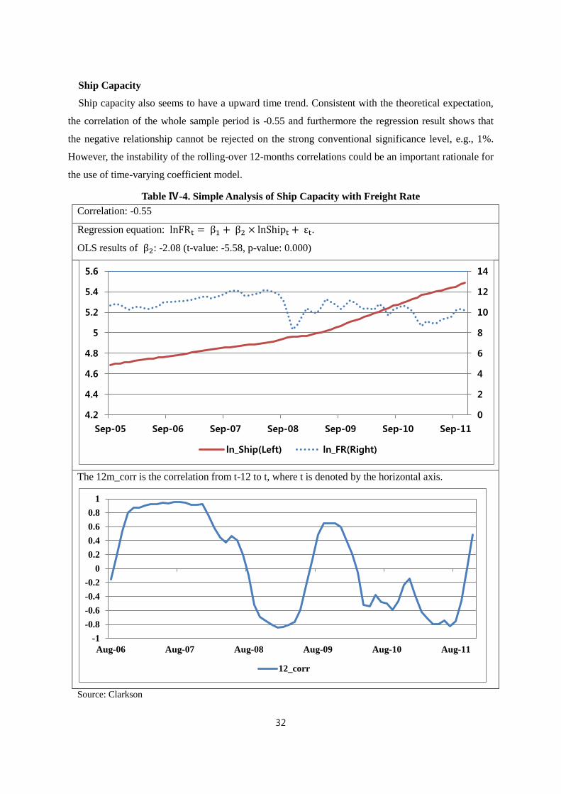
32

Ship Capacity

Ship capacity also seems to have a upward time trend. Consistent with the theoretical expectation,

the correlation of the whole sample period is -0.55 and furthermore the regression result shows that

the negative relationship cannot be rejected on the strong conventional significance level, e.g., 1%.

However, the instability of the rolling-over 12-months correlations could be an important rationale for

the use of time-varying coefficient model.

Table Ⅳ-4. Simple Analysis of Ship Capacity with Freight Rate

Correlation: -0.55

Regression equation: lnFRt = β1 + β2 × lnShipt + εt.

OLS results of β2: -2.08 (t-value: -5.58, p-value: 0.000)

The 12m_corr is the correlation from t-12 to t, where t is denoted by the horizontal axis.

Source: Clarkson

0

2

4

6

8

10

12

14

4.2

4.4

4.6

4.8

5

5.2

5.4

5.6

Sep-05 Sep-06 Sep-07 Sep-08 Sep-09 Sep-10 Sep-11

ln_Ship(Left) ln_FR(Right)

-1

-0.8

-0.6

-0.4

-0.2

0

0.2

0.4

0.6

0.8

1

Aug-06 Aug-07 Aug-08 Aug-09 Aug-10 Aug-11

12_corr

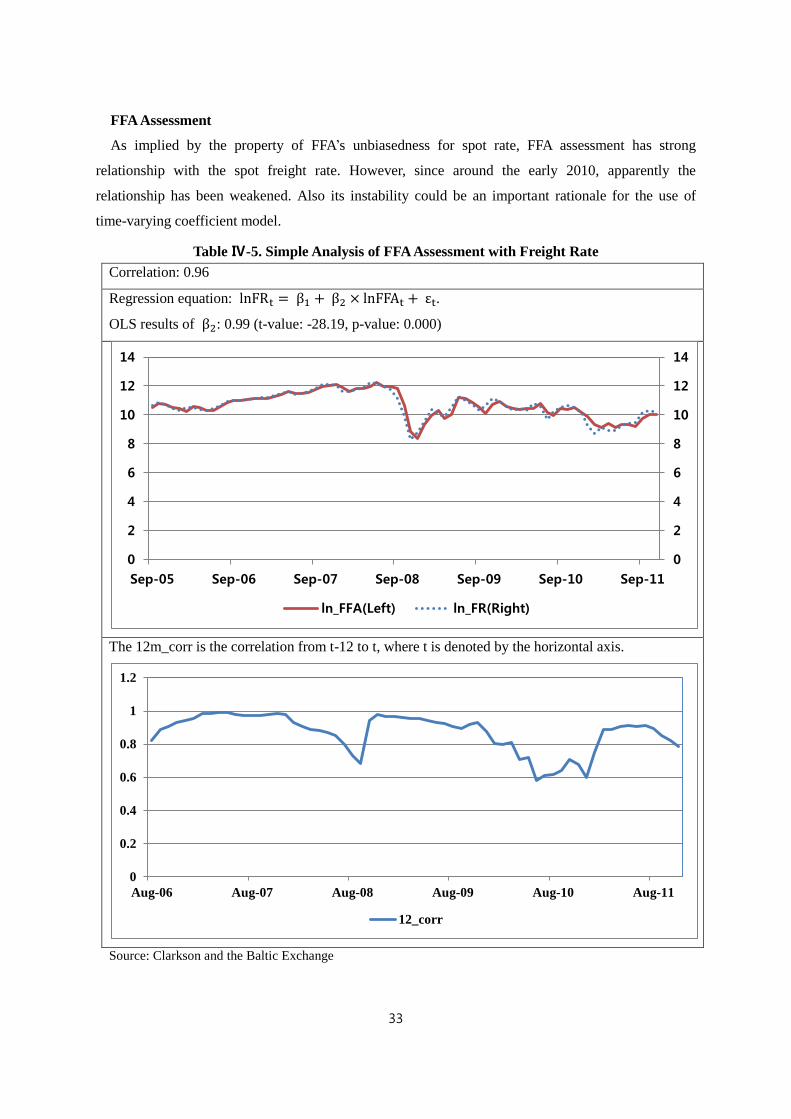
33

FFA Assessment

As implied by the property of FFA’s unbiasedness for spot rate, FFA assessment has strong

relationship with the spot freight rate. However, since around the early 2010, apparently the

relationship has been weakened. Also its instability could be an important rationale for the use of

time-varying coefficient model.

Table Ⅳ-5. Simple Analysis of FFA Assessment with Freight Rate

Correlation: 0.96

Regression equation: lnFRt = β1 + β2 × lnFFAt + εt.

OLS results of β2: 0.99 (t-value: -28.19, p-value: 0.000)

The 12m_corr is the correlation from t-12 to t, where t is denoted by the horizontal axis.

Source: Clarkson and the Baltic Exchange

0

2

4

6

8

10

12

14

0

2

4

6

8

10

12

14

Sep-05 Sep-06 Sep-07 Sep-08 Sep-09 Sep-10 Sep-11

ln_FFA(Left) ln_FR(Right)

0

0.2

0.4

0.6

0.8

1

1.2

Aug-06 Aug-07 Aug-08 Aug-09 Aug-10 Aug-11

12_corr

34

Keeping in mind the information of Table Ⅳ-3 ~ Ⅳ-5, now we perform the unit root tests for the

variables of lnFR, lnCargo, lnShip, and lnFFA. As preliminary results, they are all nonstationary in the

sense that, in the level, the null hypothesis of unit root cannot be rejected.

A popular unit root test, i.e., the augmented Dickey-Fuller test uses the following specification:78

79

Δyt = α × yt−1 + δxt + ∑ βipi=1 × Δyt−i + εt, --- (Ⅳ-2)

where xt are the exogenous regressors which may consist of constant, or a constant and trend.

Dickey and Fuller (1979) show that under the null hypothesis of a unit root, the conventional t-

statistic does not follow the conventional Student’s t-distribution, and they derive asymptotic results

and simulate critical values for various test and sample sizes.

According to the ADF (Augmented Dickey-Fuller) tests for unit root hypothesis in the below table,

all the variables are nonstationary. However, the first-differenced time series seems to be stationary in

relatively high significance level, except the case of lnShip variable.viii

Table Ⅳ-6. Results of Unit Root Test for Level Value

- xt

None Constant Constant and trend

lnFR t-value -0.29 -1.50 -2.49

p-value 0.57 0.52 0.33

lnCargo t-value 1.34 -0.90 -2.44

p-value 0.95 0.78 0.35

lnShip t-value 2.19 0.84 -1.65

p-value 0.99 0.99 0.75

lnFFA t-value -0.29 -1.34 -2.32

p-value 0.57 0.60 0.41

With respect to the nonstationarity of variables, there have been some important research results. In

contrast to the existing consensus that most of the data in dry bulk shipping markets is first difference

stationary,ix Tvedt (2003) and Adland and Cullinane (2006) argue that some data is stationary in

levels. If this is true, then the first differencing and the implied use of VAR modeling methodology,

which has been a research trend after Beenstock and Vergottis (1993), is presumably misleading.80

78

The explanations of unit root tests in this section are based on Quantitative Micro Software’s EViews 6 User’s

Guide. Also, the explanations of the tests and estimations for cointegration are based on EViews 6. 79

For AR(1) process, the original autoregressive process can be represented as follows:

yt = ρ × yt−1 + δxt + εt.

The unit root hypothesis is that ρ = 1. 80

On p.441. of Glen (2006).

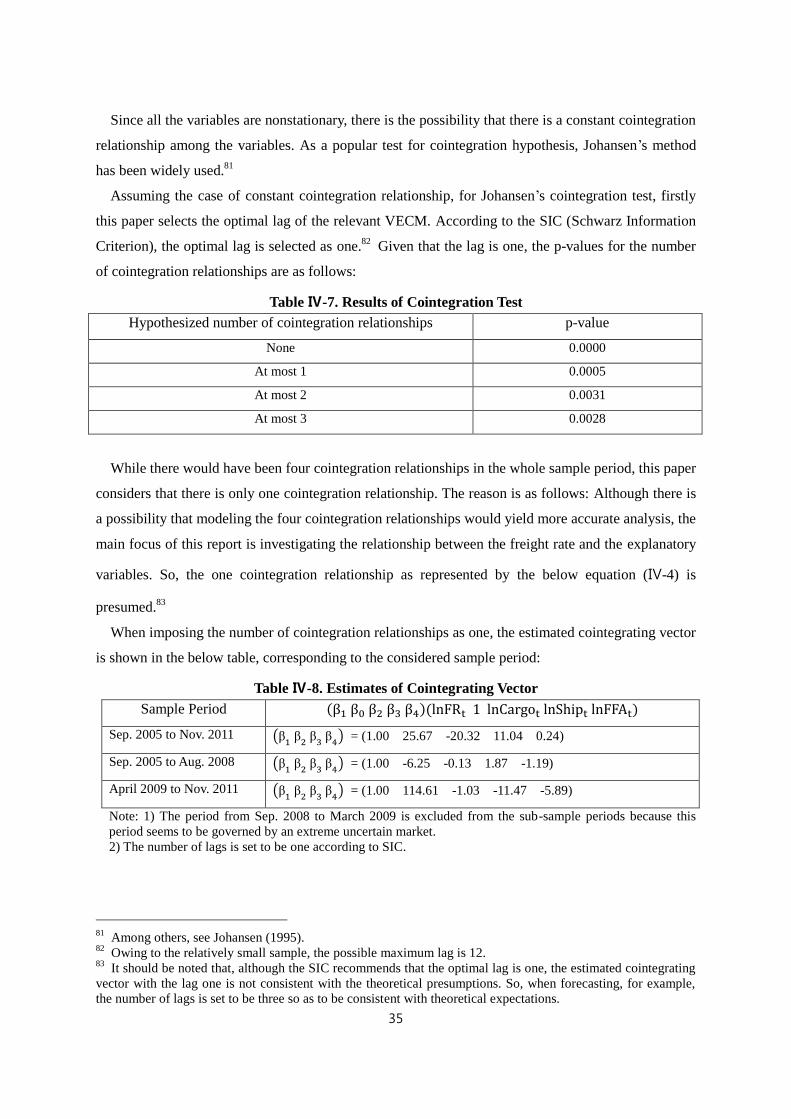
35

Since all the variables are nonstationary, there is the possibility that there is a constant cointegration

relationship among the variables. As a popular test for cointegration hypothesis, Johansen’s method

has been widely used.81

Assuming the case of constant cointegration relationship, for Johansen’s cointegration test, firstly

this paper selects the optimal lag of the relevant VECM. According to the SIC (Schwarz Information

Criterion), the optimal lag is selected as one.82

Given that the lag is one, the p-values for the number

of cointegration relationships are as follows:

Table Ⅳ-7. Results of Cointegration Test

Hypothesized number of cointegration relationships p-value

None 0.0000

At most 1 0.0005

At most 2 0.0031

At most 3 0.0028

While there would have been four cointegration relationships in the whole sample period, this paper

considers that there is only one cointegration relationship. The reason is as follows: Although there is

a possibility that modeling the four cointegration relationships would yield more accurate analysis, the

main focus of this report is investigating the relationship between the freight rate and the explanatory

variables. So, the one cointegration relationship as represented by the below equation (Ⅳ-4) is

presumed.83

When imposing the number of cointegration relationships as one, the estimated cointegrating vector

is shown in the below table, corresponding to the considered sample period:

Table Ⅳ-8. Estimates of Cointegrating Vector

Sample Period (β1 β0 β2 β3 β4)(lnFRt 1 lnCargot lnShipt lnFFAt)

Sep. 2005 to Nov. 2011 (β1 β

2 β

3 β

4) = (1.00 25.67 -20.32 11.04 0.24)

Sep. 2005 to Aug. 2008 (β1 β

2 β

3 β

4) = (1.00 -6.25 -0.13 1.87 -1.19)

April 2009 to Nov. 2011 (β1 β

2 β

3 β

4) = (1.00 114.61 -1.03 -11.47 -5.89)

Note: 1) The period from Sep. 2008 to March 2009 is excluded from the sub-sample periods because this

period seems to be governed by an extreme uncertain market.

2) The number of lags is set to be one according to SIC.

81

Among others, see Johansen (1995). 82

Owing to the relatively small sample, the possible maximum lag is 12. 83

It should be noted that, although the SIC recommends that the optimal lag is one, the estimated cointegrating

vector with the lag one is not consistent with the theoretical presumptions. So, when forecasting, for example,

the number of lags is set to be three so as to be consistent with theoretical expectations.

36

As shown in the theoretical arguments of the section Ⅳ-2, the sign of lnShip relative to lnFR in the

cointegrating vector is presumed to be the same but the signs of lnCargo and lnFFA relative to lnFR

are to be presumed to be the opposite in the cointegrating vector. However, the estimated results are

not consistent with these presumptions. That is, they differ across the considered sample periods. This

inconsistency can also be a rationale for the adoption of time-variation of the relationships among the

variables.

Ⅳ-2. Time-Varying Coefficient Model

Stopford (2009) states “identifying the underlying economic model is a vital part of the process

because it tells us what information to collect and analyse”.84

Though his subsequent explanation

partly does not reflect recent development in economic theory and econometrics (i.e., the time-

variation of the parameters), the fundamental need of model cannot disappear. That is, he insists that

the forecasting job should be helpful in taking decisions. This philosophy that forecasting the freight

rate should be conducted in a context of practical (decision-making) purpose is applied to this report.

However, particularly because this report adopts the time-varying coefficient model, it will be

different from the perspective of the ‘constant coefficient model’ literature.85

This character of time-

varying coefficient model,86

the author believes, will allow for the model user to interpret the current

phenomena more flexibly given the limited data.

In advance of defining the specification of time-series model with time-varying coefficients, we

should identify the structure which determines the dry bulk freight rate.

84

Stopford (2009) classifies the forecast job into the three different approaches such as the market report, the

forecasting model, and scenario analysis. Surely, this report belongs to the second approach of forecasting

model. However, as he says, this forecasting model based on economic model can help the first forecast job of

market report because the forecasting model can make the task of writing the market report manageable in terms

of the volume of information to be handled. That is, the forecasting model can guide the market report. 85

As another example of time-varying parameter model, the time-varying volatility model can be considered.

However, this varying volatility model with constant coefficients treats the unexplained portion as shocks so that

the varying relationship between the dependent and explanatory variables cannot be detected. In this sense, the

approach of this report, which can provide more information on the interactions of market variables, is

differentiated from that of the time-varying volatility model.

For a brief review of the time-varying volatility models in shipping freight markets, see Ko (2010) which

suggests an alternative modeling strategy of dealing with the evolution of the mixture of two extreme regimes,

one for low-volatility regime and the other for high-volatility regime. 86

The author thinks that allowing for the time variation of model parameter yields paradoxically the more exact

inference on the future than that of time-invariant model. Particularly with this aspect of forecasting, Stopford

(2009) states as follows: Rather than playing safe with a wide range, most participants give a narrow one and miss the right answer.

Because we are unwilling to reveal our ignorance by specifying the very wide range, we choose to be

precisely wrong rather than vaguely right. (on p.739. of Ibid.)

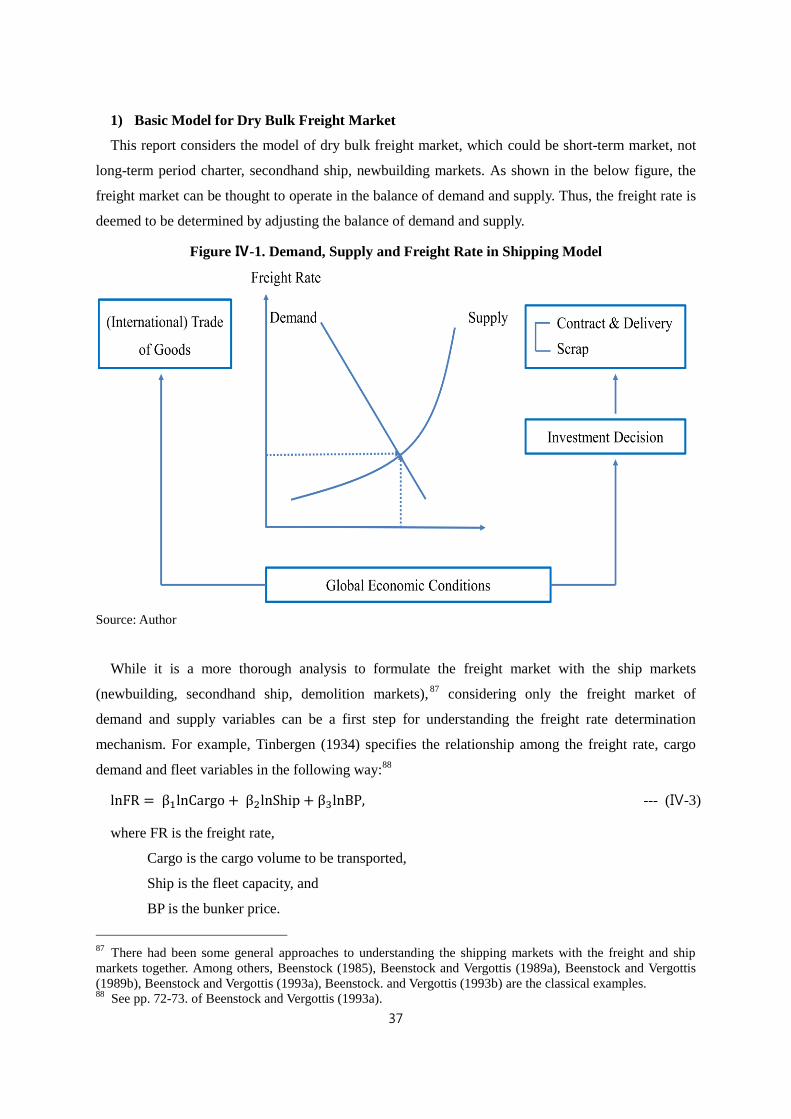
37

1) Basic Model for Dry Bulk Freight Market

This report considers the model of dry bulk freight market, which could be short-term market, not

long-term period charter, secondhand ship, newbuilding markets. As shown in the below figure, the

freight market can be thought to operate in the balance of demand and supply. Thus, the freight rate is

deemed to be determined by adjusting the balance of demand and supply.

Figure Ⅳ-1. Demand, Supply and Freight Rate in Shipping Model

Source: Author

While it is a more thorough analysis to formulate the freight market with the ship markets

(newbuilding, secondhand ship, demolition markets),87

considering only the freight market of

demand and supply variables can be a first step for understanding the freight rate determination

mechanism. For example, Tinbergen (1934) specifies the relationship among the freight rate, cargo

demand and fleet variables in the following way:88

lnFR = β1lnCargo + β2lnShip + β3lnBP, --- (Ⅳ-3)

where FR is the freight rate,

Cargo is the cargo volume to be transported,

Ship is the fleet capacity, and

BP is the bunker price.

87

There had been some general approaches to understanding the shipping markets with the freight and ship

markets together. Among others, Beenstock (1985), Beenstock and Vergottis (1989a), Beenstock and Vergottis

(1989b), Beenstock and Vergottis (1993a), Beenstock. and Vergottis (1993b) are the classical examples. 88

See pp. 72-73. of Beenstock and Vergottis (1993a).

38

The freight rate is determined with voyage contract or trip charter contract. Because the freight rate

of voyage contract includes the bunker cost but the freight rate of trip charter contract does not

include the bunker cost, when using the trip charter rate as the freight rate variable, we can drop the

term of bunker price.

However, since 1985 when the futures market had been introduced in the bulk shipping freight

market, the movements in the futures or forward markets have been influencing the physical spot

markets. Therefore, we could add the term of futures or forward information to the original freight

rate determination equation. In this report, like the equation (Ⅳ-3), we consider the following

mathematical formulation:89

lnFR = β1lnCargo + β2lnShip + β3lnFFA, --- (Ⅳ-4)

where FR is the freight rate,

Cargo is the cargo volume to be transported,

Ship is the fleet capacity, and

FFA is the freight rate assessment for the relevant underlying shipping route or basket of

routes.

The above demand/supply model for the freight rate determination is well accepted in the bulk

shipping market, mainly because the bulk shipping market is more perfect competitive than the

container shipping market.90

However, Luo, Fan and Liu (2009) show that the historical dynamics of

the container freight rate and fleet capacity are also well explained by the use of this kind of

demand/supply model approach.

89

It is notable that the freight rate can be modeled to be dependent only on the ratio of the cargo demand over

the fleet capacity like the formulation of Tvedt (2003). 90

As well known, the suppliers of container market have been allowed to form some cooperative organizations

such as conference, alliance, consortium, etc. This cooperation among the suppliers is thought to influence the

freight rate determination so that the equilibrium freight rate could deviate from the level which is purely

determined by the demand and supply variables.

39

2) Time-Varying Coefficient Model

In the above section, we assume that there is a unique relationship between the freight rate and the

explanatory variables. However, since the market forces, for example, market sentiment, can influence

the freight rate determination mechanism, there could be multiple relationships between the freight

rate and the demand/supply balance.91

Facing this multiplicity problem, if we use constant coefficient

model, we can make mistakes on the inference about the ongoing market process. Therefore, this

report considers the model with time variation of coefficients.92

For example, the estimate of cargo demand coefficient is interpreted as the elasticity of freight rate

for demand change. This is the ratio of the percentage change of freight rate to the percentage change

of cargo demand. Theoretically, this kind of elasticity could be derived from market demand curve

representing all the relevant preferences of shippers. However, largely because we could not observe

the structure of market demand, we estimate this elasticity empirically considering the relationships

with ship capacity and FFA price.93

The following explanation gives some theoretical rationales for

the time variation of coefficients respectively.94

As a result from the use of proxy variable for cargo demand, the estimates of demand elasticity

coefficient include the information for the omitted variable. For example, given all the other things

equal, if the increase in average haul occurs, then the estimate of commodity coefficient will increase

accordingly. That is, the positive pressure of cargo demand on the freight rate increases. As an

example for supply side, if the port congestion increases (i.e., the effect of fleet capacity decreases),

91

For a graphical example, see the figure on p.169 of Stopford (2009). 92

In macroeconomics, Engle and Watson (1987) argue that, due to 1) behavioral motivation, 2) unobserved

causes, 3) model misspecification, the estimated coefficients can vary by time. These possibilities could realize

in the analysis of shipping market. Also, it is notable that the strategic interactions among market participants of

shipping market make the relevant coefficient time-varying. 93

However, using the following logic (see pp. 72-73 of Beenstock and Vergottis (1993a)), we could compute

some fundamental parameters governing the supply behavior.

If we formulate the supply of shipping service as Cargo = Shipα × FRβ × FFA−γ,

then we can derive the following logarithmic equation:

lnFR = e1 × lnCargo − e2 × lnShip + e3lnFFA,

where e1 = 1 β⁄ , e2 = α β⁄ , and e3 = γ

β⁄ .

Therefore, if we estimate e1, e2 and e3, then we could calculate the parameters, α, β and γ. 94

Stopford (2009) considers this kind of parameter variation as the nature of the market. He says “When there

are two ships and two cargoes, freight rates are determined by market sentiment at auction, and economics

cannot tell us how the auction will develop. At their best shipping market models are educational in the sense

that they help decision-makers to understand in simple graphic terms what could happen, but when it comes to

predicting what will actually happen to freight rates are very blunt instruments.” (p.722. of Ibid.) Especially, he

emphasizes that in the short term the psychology is as important as fundamentals (demand and supply). (p.139.

of Ibid.)

However, regarding market sentiment, Tvedt (2011) analyses an interesting short-run freight rate formation

mechanism of VLCC market in a theoretical framework, which uses an assignment model based on two-sided

matching theory. Particularly, this paper considers the relative bargaining power of shipowner and charterer

(shipper) as an important factor for freight rate determination. Furthermore, the shipbrokers’ perception of

market psychology is also examined.

40

then the estimate of fleet coefficient will decrease. It means that the negative pressure of ship supply

on the freight rate decreases.95

Also, the slow-steaming has a similar effect with that of port

congestion because it could exhibit fleet-absorption effect, too.

In summary, this report considers the following time-varying coefficients model:

lnFRt = β0 + β1,tlnCargot + β2,tlnShipt + β3,tlnFFAt , --- (Ⅳ-5)

where FR is the freight rate,

Cargo is the cargo volume to be transported,

Ship is the fleet capacity, and

FFA is the freight rate assessment for the relevant underlying shipping route or a basket of

routes.

The above equation is a typical multiple regression model. However, as shown in Table Ⅳ-6, all

the variables seem to be nonstationary. So, if there are some relationships among these variables, we

can say that there is a time-varying cointegration relationship among the variables.96

Before analysing

this kind of cointegration relationship, we should argue that they can be formulated by the VAR model.

In order to use the VAR model, the variables of ship capacity, cargo volume, FFA assessment and

freight rate should be treated as endogenous.97

While the ship capacity, FFA assessment and freight

rate can be easily treated as endogenous, the cargo volume is controversially vague in the degree of

endogeneity. Beenstock and Vergottis (1993) treat it as exogenous and most of shipping textbooks

consider the price elasticity of demand as very inelastic, which means that the cargo volume can be

95

Similarly, if the time spent in ballast or repairs increases, then the fleet coefficient estimate will decrease. 96

For the example of the application of time-invariant cointegration method to shipping market, among others,

see Veenstra and Franses (1997), Glen (1997), and Hale and Vanags (1992). 97

In methodological aspects, the endogeneity is very complex. For example, if we considered this endogeneity

as a strategic element of market players, then the below forecasting model could become less useful. The reason

is as follows: Suppose that the proposed model of this report is accurate and some of relevant market players can

influence the explanatory variables. Then the player wants to control the variables of interest so that the

underlying system will change into a different one, which pays more to them. As a result, the estimates of the

parameters and their inferences will be less accurate as the time passes. (For another example, see pp.704-705.

of Stopford (2009).)

This kind of complexity on the statistical regularity is well-known as “Goodhart’s Law”. (Goodhart (1975a) and

Goodhart (1975b)) This theorem says “any observed statistical regularity will tend to collapse once pressure is

placed upon it for control purposes”. (See p.4. of Chrystal and Mizen (2001).) This result of the feedback

mechanism between human intention and observation of objective phenomenon can be interpreted in the lens of

more in-depth scientific philosophy, the Heisenberg Uncertainty Principle. “This states, in the context of

quantum physics, that the observation of a system fundamentally disturbs it. Hence, the process of observing an

electron, which requires that a proton of light should bounce off it and pass through a microscope to the eye,

alters the characteristics of the physical environment being observed because the impact of the proton on the

electron will change its momentum. A system cannot be observed without a change to the system itself being

introduced” (See p.11. of Ibid.)

41

thought to be an exogenous variable. Furthermore, the uncertainty of cargo volume is almost due to its

own uncertainty.98

However, I believe, in both theory and practice, there is no sufficiently acceptable

rationale to exclude the possibility that the freight rate will affect the transportation demand of

commodities. Therefore, including the cargo volume variable into VAR model as an endogenous one

and thus conducting the various analyses based on VAR or VECM model could be more informative

than treating it as exogenous.99

100

101

The above dry bulk freight rate model with time-varying cointegraion relationship is a kind of

structural model. This approach to modeling shipping market is like the structural model of Beenstock

and Vergottis (1993), while there are many differences especially in the process of deriving the

structure of shipping market. As Glen (2006) noted, since the publication of Beenstock and Vergottis

(1993), “there has been an implicit rejection of the use of structural models of the type found in

Beenstock and Vergottis.”102

That is, “the recent research agenda has shifted away from the

estimation of large econometric models of shipping markets, and towards examining reduced form

dynamic relations using relatively new methodologies generated by” cointegration analysis.103

This kind of marriage between structural model and nonstructural multivariate time-series analysis

has been observed in other research fields. For example, dynamic stochastic general equilibrium

(DSGE) model in macroeconometrics is based on both the structural theory and relevant time-series

analysis. Furthermore, this DSGE model is used as a forecasting tool.104

98

Refer to pp.31-32 of Rim, Kim and Ko (2010). 99

For pro-exogeneity for cargo demand, Glen’s (2006) survey paper says that the literature gives the reliance of

zero cargo demand elasticity. (See line 1-2 of p.441. of Ibid.) But, Adland and Strandenes (2007) suggest a

literature strand which argues for pro-endogeneity for cargo demand. For example, when the freight rate is high,

there could be substitute effect in the used commodity itself (e.g., from oil to coal) or transportation mode (e.g.

from ship to pipeline). (See pp.193-194. of Ibid.) 100

Particularly at monthly frequency, the cargo volume could be influenced by other variables. For example,

suppose that a big shipper is involved in the freight derivatives market, so his payoff will be proportionally

bigger to the increase of the future freight rate when the freight rate is above some level. Facing this incentive, if

the current freight rate is under the given level, he tries to push more the cargo offer in the market with an

appropriate inventory management strategy in order to increase the future settlement price. So, there will be

some positive pressure on the freight rate. This thought experiment suggests a possibility of the endogeneity of

cargo volume. 101

As shown in Figure Ⅳ-1, the cargo volume depends on the world economy and commodity trades at the

time. So, the more exact understanding of the dynamics of cargo variable requires the analysis of the world-wide

macroeconomics and international trades. In this respect, the shipping economics can be thought to face more

complex phenomenon than macroeconomics. 102

On p.432 of Glen (2006). 103

On p.435 of Ibid. 104

For more detail, refer to Diebold (1998) or chapter 14 of Diebold and Rudebusch (1999). For a different

perspective on this issue, refer to Hoover (2006).

42

Ⅴ. Estimation and In-Sample/Out-of-Sample Forecasting with Evaluation

Ⅴ-1. Estimation Results of Time-Varying Coefficient Model105

1) State-Space Models and the Kalman Filter: Application to Time-Varying Coefficient Model

Based on the model of the section Ⅳ-2, we consider the following time-varying coefficient model:

lnFRt = β0 + β1,tlnCargot + β2,tlnShipt + β3,tlnFFAt + εt , εt ~ iidN(0, σε2). --- (Ⅴ-1)

β1,t = β1,t−1 + ω1t, ω1t ~ iidN(0, σω12 ). --- (Ⅴ-2)

β2,t = β2,t−1 + ω2t, ω2t ~ iidN(0, σω22 ). --- (Ⅴ-3)

β3,t = β3,t−1 + ω3t, ω3t ~ iidN(0, σω32 ). --- (Ⅴ-4)

It is notable that, although the dynamic mechanism of coefficient is treated as a random walk, it

will be understood more deeply by using a set of explanatory variables for the dynamics of relevant

coefficient.106

For example, as mentioned above, the fleet coefficient could depend on the port

congestion, slow-steaming degree, time in ballast, fuel price, etc.

The state-space model in matrix form is as follows:

[Measurement equation]

yt = β0 + xtβt + εt, εt ~ iidN(0, R), --- (Ⅴ-5)

[Transition equation]

βt = Fβt−1 + ωt, ωt ~ iidN(0, Q), --- (Ⅴ-6)

where yt = lnFRt,

xt = [lnCargot lnShipt lnFFAt],

βt = [β1,t β2,t β3,t]′,

F = [1 0 00 1 00 0 1

],

R = σε2, Q= [

σω12 0 0

0 σω22 0

0 0 σω32

].

For notational convenience, let us define the following terms:

105

Relating to the state-space model and its estimation, this section is based on the explanation of pp.19-30. of

Kim and Nelson (1999). 106

For an example of application in other field, see Brown, Song and McGillivray (1997) as noted in the

section Ⅲ-1 of this report.

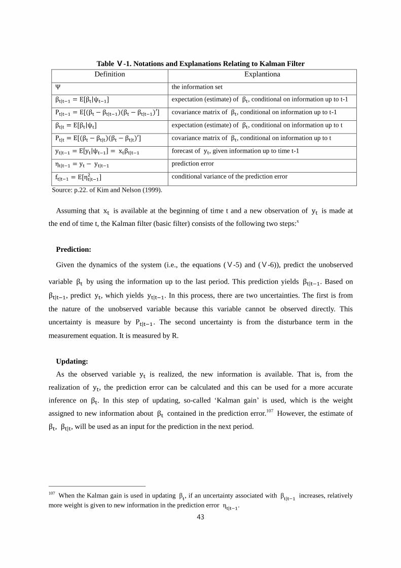
43

Table Ⅴ-1. Notations and Explanations Relating to Kalman Filter

Definition Explantiona

Ψ the information set

βt|t−1 = E[βt|ψt−1] expectation (estimate) of βt, conditional on information up to t-1

Pt|t−1 = E[(βt − βt|t−1)(βt − βt|t−1)′] covariance matrix of βt, conditional on information up to t-1

βt|t = E[βt|ψt] expectation (estimate) of βt, conditional on information up to t

Pt|t = E[(βt − βt|t)(βt − βt|t)′] covariance matrix of βt, conditional on information up to t

yt|t−1 = E[yt|ψt−1] = xtβt|t−1 forecast of yt, given information up to time t-1

ηt|t−1 = yt − yt|t−1 prediction error

ft|t−1 = E[ηt|t−12 ] conditional variance of the prediction error

Source: p.22. of Kim and Nelson (1999).

Assuming that xt is available at the beginning of time t and a new observation of yt is made at

the end of time t, the Kalman filter (basic filter) consists of the following two steps:x

Prediction:

Given the dynamics of the system (i.e., the equations (Ⅴ-5) and (Ⅴ-6)), predict the unobserved

variable βt by using the information up to the last period. This prediction yields βt|t−1. Based on

βt|t−1, predict yt, which yields yt|t−1. In this process, there are two uncertainties. The first is from

the nature of the unobserved variable because this variable cannot be observed directly. This

uncertainty is measure by Pt|t−1 . The second uncertainty is from the disturbance term in the

measurement equation. It is measured by R.

Updating:

As the observed variable yt is realized, the new information is available. That is, from the

realization of yt, the prediction error can be calculated and this can be used for a more accurate

inference on βt. In this step of updating, so-called ‘Kalman gain’ is used, which is the weight

assigned to new information about βt contained in the prediction error.107

However, the estimate of

βt, βt|t, will be used as an input for the prediction in the next period.

107

When the Kalman gain is used in updating βt, if an uncertainty associated with β

t|t−1 increases, relatively

more weight is given to new information in the prediction error ηt|t−1

.

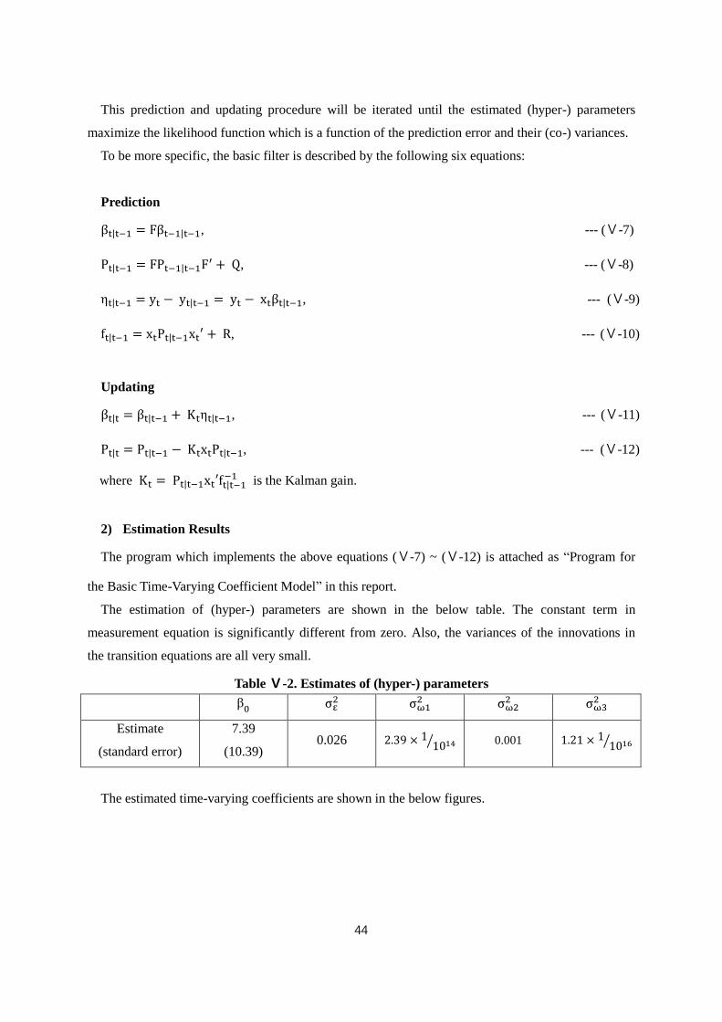
44

This prediction and updating procedure will be iterated until the estimated (hyper-) parameters

maximize the likelihood function which is a function of the prediction error and their (co-) variances.

To be more specific, the basic filter is described by the following six equations:

Prediction

βt|t−1 = Fβt−1|t−1, --- (Ⅴ-7)

Pt|t−1 = FPt−1|t−1F′ + Q, --- (Ⅴ-8)

ηt|t−1 = yt − yt|t−1 = yt − xtβt|t−1, --- (Ⅴ-9)

ft|t−1 = xtPt|t−1xt′ + R, --- (Ⅴ-10)

Updating

βt|t = βt|t−1 + Ktηt|t−1, --- (Ⅴ-11)

Pt|t = Pt|t−1 − KtxtPt|t−1, --- (Ⅴ-12)

where Kt = Pt|t−1xt′ft|t−1−1 is the Kalman gain.

2) Estimation Results

The program which implements the above equations (Ⅴ-7) ~ (Ⅴ-12) is attached as “Program for

the Basic Time-Varying Coefficient Model” in this report.

The estimation of (hyper-) parameters are shown in the below table. The constant term in

measurement equation is significantly different from zero. Also, the variances of the innovations in

the transition equations are all very small.

Table Ⅴ-2. Estimates of (hyper-) parameters

β0 σε

2 σω12 σω2

2 σω32

Estimate

(standard error)

7.39

(10.39) 0.026 2.39 × 1

1014⁄ 0.001 1.21 × 11016⁄

The estimated time-varying coefficients are shown in the below figures.

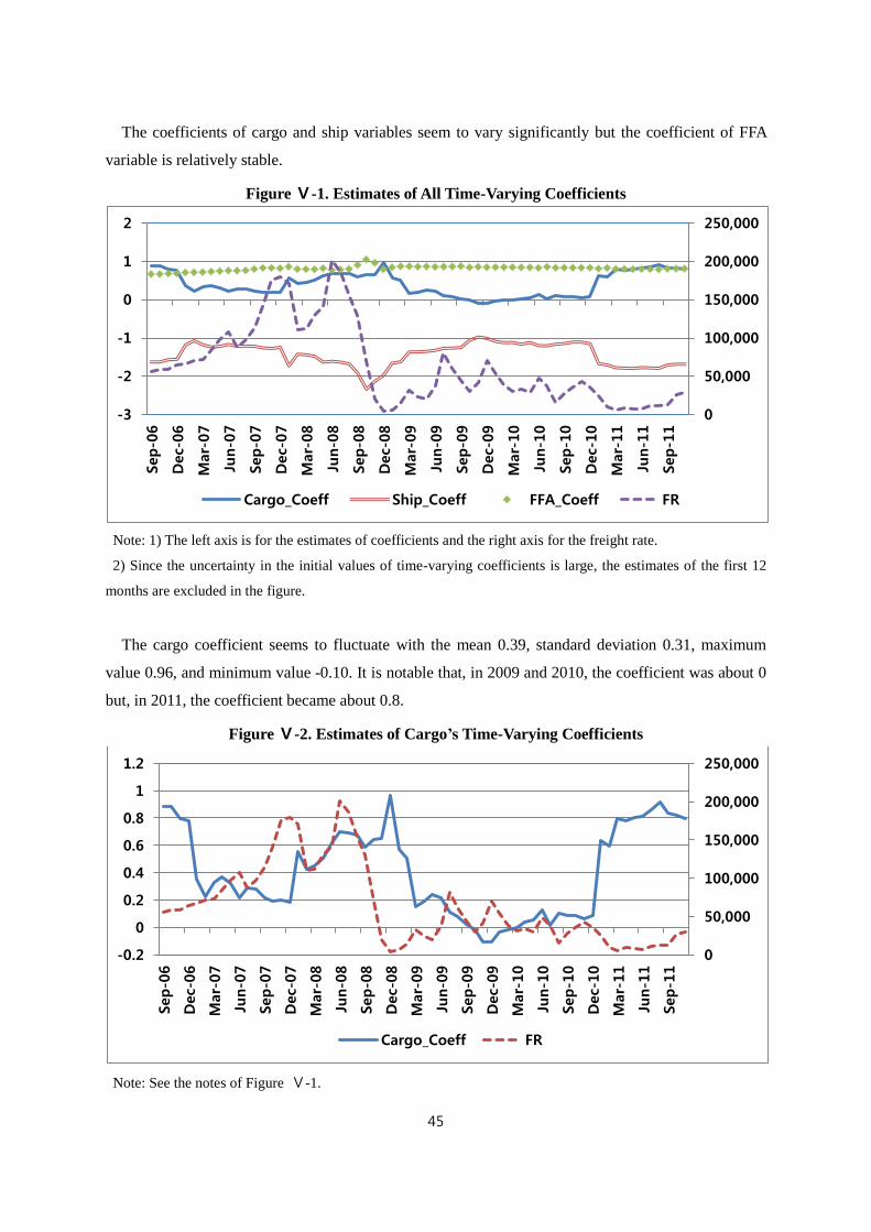
45

The coefficients of cargo and ship variables seem to vary significantly but the coefficient of FFA

variable is relatively stable.

Figure Ⅴ-1. Estimates of All Time-Varying Coefficients

Note: 1) The left axis is for the estimates of coefficients and the right axis for the freight rate.

2) Since the uncertainty in the initial values of time-varying coefficients is large, the estimates of the first 12

months are excluded in the figure.

The cargo coefficient seems to fluctuate with the mean 0.39, standard deviation 0.31, maximum

value 0.96, and minimum value -0.10. It is notable that, in 2009 and 2010, the coefficient was about 0

but, in 2011, the coefficient became about 0.8.

Figure Ⅴ-2. Estimates of Cargo’s Time-Varying Coefficients

Note: See the notes of Figure Ⅴ-1.

0

50,000

100,000

150,000

200,000

250,000

-3

-2

-1

0

1

2

Sep-0

6

Dec-

06

Mar-

07

Jun-0

7

Sep-0

7

Dec-

07

Mar-

08

Jun-0

8

Sep-0

8

Dec-

08

Mar-

09

Jun-0

9

Sep-0

9

Dec-

09

Mar-

10

Jun-1

0

Sep-1

0

Dec-

10

Mar-

11

Jun-1

1

Sep-1

1

Cargo_Coeff Ship_Coeff FFA_Coeff FR

0

50,000

100,000

150,000

200,000

250,000

-0.2

0

0.2

0.4

0.6

0.8

1

1.2

Sep-0

6

Dec-

06

Mar-

07

Jun-0

7

Sep-0

7

Dec-

07

Mar-

08

Jun-0

8

Sep-0

8

Dec-

08

Mar-

09

Jun-0

9

Sep-0

9

Dec-

09

Mar-

10

Jun-1

0

Sep-1

0

Dec-

10

Mar-

11

Jun-1

1

Sep-1

1

Cargo_Coeff FR

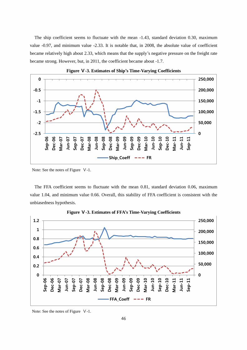
46

The ship coefficient seems to fluctuate with the mean -1.43, standard deviation 0.30, maximum

value -0.97, and minimum value -2.33. It is notable that, in 2008, the absolute value of coefficient

became relatively high about 2.33, which means that the supply’s negative pressure on the freight rate

became strong. However, but, in 2011, the coefficient became about -1.7.

Figure Ⅴ-3. Estimates of Ship’s Time-Varying Coefficients

Note: See the notes of Figure Ⅴ-1.

The FFA coefficient seems to fluctuate with the mean 0.81, standard deviation 0.06, maximum

value 1.04, and minimum value 0.66. Overall, this stability of FFA coefficient is consistent with the

unbiasedness hypothesis.

Figure Ⅴ-3. Estimates of FFA’s Time-Varying Coefficients

Note: See the notes of Figure Ⅴ-1.

0

50,000

100,000

150,000

200,000

250,000

-2.5

-2

-1.5

-1

-0.5

0

Sep-0

6

Dec-

06

Mar-

07

Jun-0

7

Sep-0

7

Dec-

07

Mar-

08

Jun-0

8

Sep-0

8

Dec-

08

Mar-

09

Jun-0

9

Sep-0

9

Dec-

09

Mar-

10

Jun-1

0

Sep-1

0

Dec-

10

Mar-

11

Jun-1

1

Sep-1

1

Ship_Coeff FR

0

50,000

100,000

150,000

200,000

250,000

0

0.2

0.4

0.6

0.8

1

1.2

Sep-0

6

Dec-

06

Mar-

07

Jun-0

7

Sep-0

7

Dec-

07

Mar-

08

Jun-0

8

Sep-0

8

Dec-

08

Mar-

09

Jun-0

9

Sep-0

9

Dec-

09

Mar-

10

Jun-1

0

Sep-1

0

Dec-

10

Mar-

11

Jun-1

1

Sep-1

1

FFA_Coeff FR

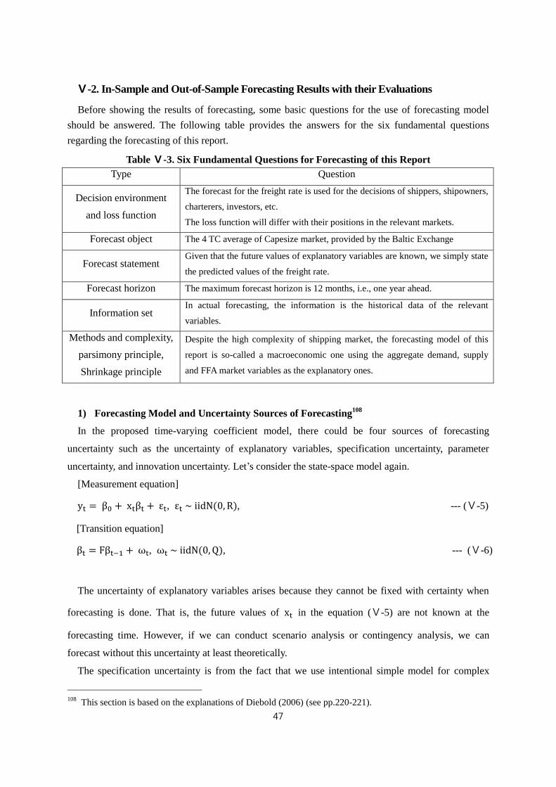
47

Ⅴ-2. In-Sample and Out-of-Sample Forecasting Results with their Evaluations

Before showing the results of forecasting, some basic questions for the use of forecasting model

should be answered. The following table provides the answers for the six fundamental questions

regarding the forecasting of this report.

Table Ⅴ-3. Six Fundamental Questions for Forecasting of this Report

Type Question

Decision environment

and loss function

The forecast for the freight rate is used for the decisions of shippers, shipowners,

charterers, investors, etc.

The loss function will differ with their positions in the relevant markets.

Forecast object The 4 TC average of Capesize market, provided by the Baltic Exchange

Forecast statement Given that the future values of explanatory variables are known, we simply state

the predicted values of the freight rate.

Forecast horizon The maximum forecast horizon is 12 months, i.e., one year ahead.

Information set In actual forecasting, the information is the historical data of the relevant

variables.

Methods and complexity,

parsimony principle,

Shrinkage principle

Despite the high complexity of shipping market, the forecasting model of this

report is so-called a macroeconomic one using the aggregate demand, supply

and FFA market variables as the explanatory ones.

1) Forecasting Model and Uncertainty Sources of Forecasting108

In the proposed time-varying coefficient model, there could be four sources of forecasting

uncertainty such as the uncertainty of explanatory variables, specification uncertainty, parameter

uncertainty, and innovation uncertainty. Let’s consider the state-space model again.

[Measurement equation]

yt = β0 + xtβt + εt, εt ~ iidN(0, R), --- (Ⅴ-5)

[Transition equation]

βt = Fβt−1 + ωt, ωt ~ iidN(0, Q), --- (Ⅴ-6)

The uncertainty of explanatory variables arises because they cannot be fixed with certainty when

forecasting is done. That is, the future values of xt in the equation (Ⅴ-5) are not known at the

forecasting time. However, if we can conduct scenario analysis or contingency analysis, we can

forecast without this uncertainty at least theoretically.

The specification uncertainty is from the fact that we use intentional simple model for complex

108

This section is based on the explanations of Diebold (2006) (see pp.220-221).

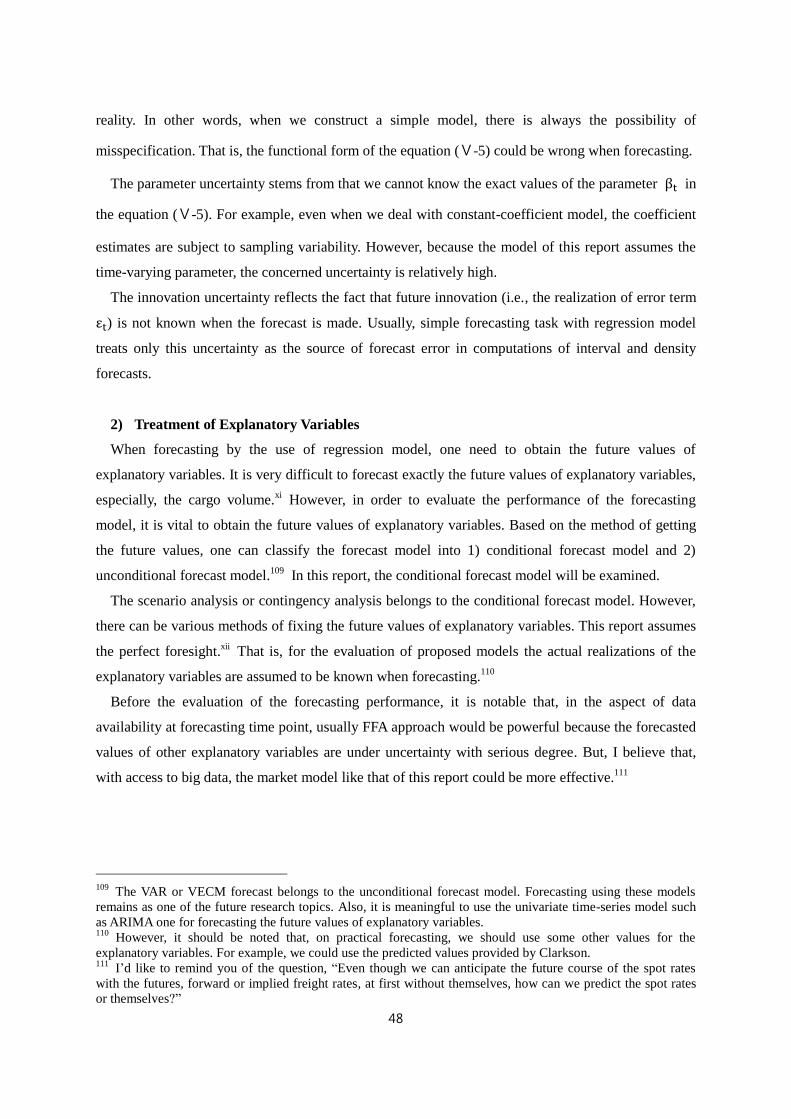
48

reality. In other words, when we construct a simple model, there is always the possibility of

misspecification. That is, the functional form of the equation (Ⅴ-5) could be wrong when forecasting.

The parameter uncertainty stems from that we cannot know the exact values of the parameter βt in

the equation (Ⅴ-5). For example, even when we deal with constant-coefficient model, the coefficient

estimates are subject to sampling variability. However, because the model of this report assumes the

time-varying parameter, the concerned uncertainty is relatively high.

The innovation uncertainty reflects the fact that future innovation (i.e., the realization of error term

εt) is not known when the forecast is made. Usually, simple forecasting task with regression model

treats only this uncertainty as the source of forecast error in computations of interval and density

forecasts.

2) Treatment of Explanatory Variables

When forecasting by the use of regression model, one need to obtain the future values of

explanatory variables. It is very difficult to forecast exactly the future values of explanatory variables,

especially, the cargo volume.xi However, in order to evaluate the performance of the forecasting

model, it is vital to obtain the future values of explanatory variables. Based on the method of getting

the future values, one can classify the forecast model into 1) conditional forecast model and 2)

unconditional forecast model.109

In this report, the conditional forecast model will be examined.

The scenario analysis or contingency analysis belongs to the conditional forecast model. However,

there can be various methods of fixing the future values of explanatory variables. This report assumes

the perfect foresight.xii

That is, for the evaluation of proposed models the actual realizations of the

explanatory variables are assumed to be known when forecasting.110

Before the evaluation of the forecasting performance, it is notable that, in the aspect of data

availability at forecasting time point, usually FFA approach would be powerful because the forecasted

values of other explanatory variables are under uncertainty with serious degree. But, I believe that,

with access to big data, the market model like that of this report could be more effective.111

109

The VAR or VECM forecast belongs to the unconditional forecast model. Forecasting using these models

remains as one of the future research topics. Also, it is meaningful to use the univariate time-series model such

as ARIMA one for forecasting the future values of explanatory variables. 110

However, it should be noted that, on practical forecasting, we should use some other values for the

explanatory variables. For example, we could use the predicted values provided by Clarkson. 111

I’d like to remind you of the question, “Even though we can anticipate the future course of the spot rates

with the futures, forward or implied freight rates, at first without themselves, how can we predict the spot rates

or themselves?”

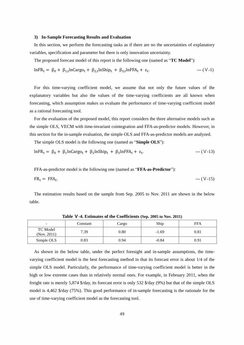
49

3) In-Sample Forecasting Results and Evaluation

In this section, we perform the forecasting tasks as if there are no the uncertainties of explanatory

variables, specification and parameter but there is only innovation uncertainty.

The proposed forecast model of this report is the following one (named as “TC Model”):

lnFRt = β0 + β1,tlnCargot + β2,tlnShipt + β3,tlnFFAt + εt. --- (Ⅴ-1)

For this time-varying coefficient model, we assume that not only the future values of the

explanatory variables but also the values of the time-varying coefficients are all known when

forecasting, which assumption makes us evaluate the performance of time-varying coefficient model

as a rational forecasting tool.

For the evaluation of the proposed model, this report considers the three alternative models such as

the simple OLS, VECM with time-invariant cointegration and FFA-as-predictor models. However, in

this section for the in-sample evaluation, the simple OLS and FFA-as-predictor models are analyzed.

The simple OLS model is the following one (named as “Simple OLS”):

lnFRt = β0 + β1lnCargot + β2lnShipt + β3lnFFAt + εt. --- (Ⅴ-13)

FFA-as-predictor model is the following one (named as “FFA-as-Predictor”):

FRt = FFAt. --- (Ⅴ-15)

The estimation results based on the sample from Sep. 2005 to Nov. 2011 are shown in the below

table.

Table Ⅴ-4. Estimates of the Coefficients (Sep. 2005 to Nov. 2011)

- Constant Cargo Ship FFA

TC Model

(Nov. 2011) 7.39 0.80 -1.69 0.81

Simple OLS 0.83 0.94 -0.84 0.91

As shown in the below table, under the perfect foresight and in-sample assumptions, the time-

varying coefficient model is the best forecasting method in that its forecast error is about 1/4 of the

simple OLS model. Particularly, the performance of time-varying coefficient model is better in the

high or low extreme cases than in relatively normal ones. For example, in February 2011, when the

freight rate is merely 5,874 $/day, its forecast error is only 532 $/day (9%) but that of the simple OLS

model is 4,462 $/day (75%). This good performance of in-sample forecasting is the rationale for the

use of time-varying coefficient model as the forecasting tool.

50

Table-5. In-Sample Forecasting Results and Evaluation (Forecasting Horizon is 12 months) - Actual FR TC Model Simple OLS FFA-as-Predictor

Dec-10 25,162 26,008

(946)

24,818

(344)

26,078

(916)

Jan-11 10,217 12,216

(1,999)

16,332

(6,115)

19,250

(9,033)

Feb-11 5,874 6,406

(532)

10,336

(4,462)

11,364

(5,490)

Mar-11 8,991 7,820

(1,171)

9,184

(193)

9,438

(447)

Apr-11 7,665 8,124

(459)

11,241

(3,576)

11,736

(4,071)

May-11 7,372 7,165

(207)

9,228

(1,856)

9,157

(1,785)

Jun-11 10,780 9,972

(808)

11,221

(441)

11,325

(545)

Jul-11 11,862 11,241

(621)

11,316

(546)

10,975

(-887)

Aug-11 13,142 12,139

(1,003)

10,224

(2,918)

9,667

(-3,475)

Sep-11 26,170 23,646

(2,524)

17,029

(9,141)

17,242

(-8,928)

Oct-11 29,373 28,793

(580)

20,722

(8,651)

21,742

(-7,631)

Nov-11 26,160 27,253

(1,093)

21,961

(4,199)

22,208

(-3,952)

Monthly average of forecast error

(ratio to actual rate)

987

(6%)

3,537

(23%)

3,930

(26%)

Note: ( ) is the difference, (forecast – actual FR).

4) Out-of-Sample Forecasting Results and Evaluation

In this section, we consider the case where we don’t know the time-varying coefficients but, as in

the previous section 3), we know the future values of explanatory variables. Also, additionally we will

show the results of VECM.

That is, in addition to the time-varying coefficient, simple OLS and FFA-as-predictor models, the

freight rate equation of the relevant VECM with time-invariant cointegration, which is the following

one (named as “VECM with TI_CI”), is estimated:112

ΔlnFRt = α[β0 1 β2 β3 β4]

[

1lnCargot−1

lnShipt−1

lnFFAt−1

lnFRt−1 ]

+ ∑ ΓiΔxt−ip−1i=1 + c + εt, --- (Ⅴ-14)

where xt = [lnCargot lnShipt lnFFAt lnFRt] and

βi, Γi, and c are the relevant coefficient terms.

112

The optimal lag is set to be three (see the footnote 83).

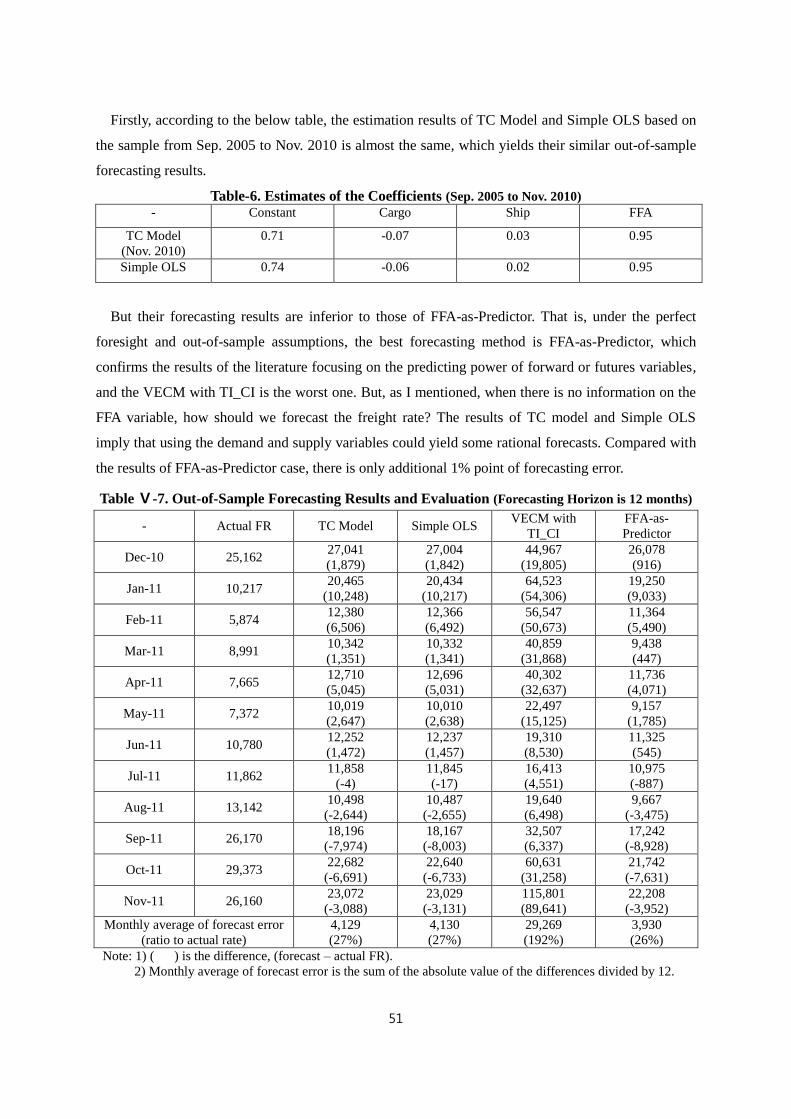
51

Firstly, according to the below table, the estimation results of TC Model and Simple OLS based on

the sample from Sep. 2005 to Nov. 2010 is almost the same, which yields their similar out-of-sample

forecasting results.

Table-6. Estimates of the Coefficients (Sep. 2005 to Nov. 2010) - Constant Cargo Ship FFA

TC Model

(Nov. 2010)

0.71 -0.07 0.03 0.95

Simple OLS 0.74 -0.06 0.02 0.95

But their forecasting results are inferior to those of FFA-as-Predictor. That is, under the perfect

foresight and out-of-sample assumptions, the best forecasting method is FFA-as-Predictor, which

confirms the results of the literature focusing on the predicting power of forward or futures variables,

and the VECM with TI_CI is the worst one. But, as I mentioned, when there is no information on the

FFA variable, how should we forecast the freight rate? The results of TC model and Simple OLS

imply that using the demand and supply variables could yield some rational forecasts. Compared with

the results of FFA-as-Predictor case, there is only additional 1% point of forecasting error.

Table Ⅴ-7. Out-of-Sample Forecasting Results and Evaluation (Forecasting Horizon is 12 months)

- Actual FR TC Model Simple OLS VECM with

TI_CI

FFA-as-

Predictor

Dec-10 25,162 27,041

(1,879)

27,004

(1,842)

44,967

(19,805)

26,078

(916)

Jan-11 10,217 20,465

(10,248)

20,434

(10,217)

64,523

(54,306)

19,250

(9,033)

Feb-11 5,874 12,380

(6,506)

12,366

(6,492)

56,547

(50,673)

11,364

(5,490)

Mar-11 8,991 10,342

(1,351)

10,332

(1,341)

40,859

(31,868)

9,438

(447)

Apr-11 7,665 12,710

(5,045)

12,696

(5,031)

40,302

(32,637)

11,736

(4,071)

May-11 7,372 10,019

(2,647)

10,010

(2,638)

22,497

(15,125)

9,157

(1,785)

Jun-11 10,780 12,252

(1,472)

12,237

(1,457)

19,310

(8,530)

11,325

(545)

Jul-11 11,862 11,858

(-4)

11,845

(-17)

16,413

(4,551)

10,975

(-887)

Aug-11 13,142 10,498

(-2,644)

10,487

(-2,655)

19,640

(6,498)

9,667

(-3,475)

Sep-11 26,170 18,196

(-7,974)

18,167

(-8,003)

32,507

(6,337)

17,242

(-8,928)

Oct-11 29,373 22,682

(-6,691)

22,640

(-6,733)

60,631

(31,258)

21,742

(-7,631)

Nov-11 26,160 23,072

(-3,088)

23,029

(-3,131)

115,801

(89,641)

22,208

(-3,952)

Monthly average of forecast error

(ratio to actual rate)

4,129

(27%)

4,130

(27%)

29,269

(192%)

3,930

(26%)

Note: 1) ( ) is the difference, (forecast – actual FR).

2) Monthly average of forecast error is the sum of the absolute value of the differences divided by 12.

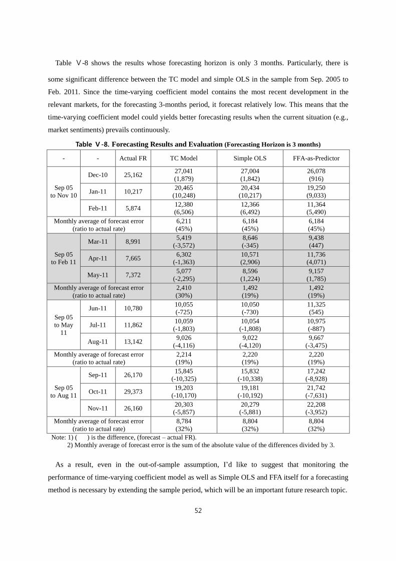
52

Table Ⅴ-8 shows the results whose forecasting horizon is only 3 months. Particularly, there is

some significant difference between the TC model and simple OLS in the sample from Sep. 2005 to

Feb. 2011. Since the time-varying coefficient model contains the most recent development in the

relevant markets, for the forecasting 3-months period, it forecast relatively low. This means that the

time-varying coefficient model could yields better forecasting results when the current situation (e.g.,

market sentiments) prevails continuously.

Table Ⅴ-8. Forecasting Results and Evaluation (Forecasting Horizon is 3 months)

- - Actual FR TC Model Simple OLS FFA-as-Predictor

Sep 05

to Nov 10

Dec-10 25,162 27,041

(1,879)

27,004

(1,842)

26,078

(916)

Jan-11 10,217 20,465

(10,248)

20,434

(10,217)

19,250

(9,033)

Feb-11 5,874 12,380

(6,506)

12,366

(6,492)

11,364

(5,490)

Monthly average of forecast error

(ratio to actual rate)

6,211

(45%)

6,184

(45%)

6,184

(45%)

Sep 05

to Feb 11

Mar-11 8,991 5,419

(-3,572)

8,646

(-345)

9,438

(447)

Apr-11 7,665 6,302

(-1,363)

10,571

(2,906)

11,736

(4,071)

May-11 7,372 5,077

(-2,295)

8,596

(1,224)

9,157

(1,785)

Monthly average of forecast error

(ratio to actual rate)

2,410

(30%)

1,492

(19%)

1,492

(19%)

Sep 05

to May

11

Jun-11 10,780 10,055

(-725)

10,050

(-730)

11,325

(545)

Jul-11 11,862 10,059

(-1,803)

10,054

(-1,808)

10,975

(-887)

Aug-11 13,142 9,026

(-4,116)

9,022

(-4,120)

9,667

(-3,475)

Monthly average of forecast error

(ratio to actual rate)

2,214

(19%)

2,220

(19%)

2,220

(19%)

Sep 05

to Aug 11

Sep-11 26,170 15,845

(-10,325)

15,832

(-10,338)

17,242

(-8,928)

Oct-11 29,373 19,203

(-10,170)

19,181

(-10,192)

21,742

(-7,631)

Nov-11 26,160 20,303

(-5,857)

20,279

(-5,881)

22,208

(-3,952)

Monthly average of forecast error

(ratio to actual rate)

8,784

(32%)

8,804

(32%)

8,804

(32%)

Note: 1) ( ) is the difference, (forecast – actual FR).

2) Monthly average of forecast error is the sum of the absolute value of the differences divided by 3.

As a result, even in the out-of-sample assumption, I’d like to suggest that monitoring the

performance of time-varying coefficient model as well as Simple OLS and FFA itself for a forecasting

method is necessary by extending the sample period, which will be an important future research topic.

53

Ⅵ. Conclusion

Ⅵ-1. Summary

Up to now, this report suggests a time-varying coefficient model as one forecasting tool for the dry

bulk freight rate. For the market practitioners without appropriate knowledge of econometrics, it starts

with the basic concepts of time-series analysis. And then, to position the report in the relevant

literature, it reviews the other fields such as Macroeconomics and Finance focusing on the

cointegration, time-variation of parameters, out-of-sample forecasting, etc., and studies the shipping

economics literature about forecasting dry bulk freight rate. In the Chapter Ⅵ, the data set is

explained and then the theoretical time-varying coefficient model for the empirical analysis is

suggested.

Chapter Ⅴ shows the estimation results and the forecasting performance. In the perfect foresight

and in-sample assumptions, the proposed time-varying coefficient model is the best forecasting tool

relative to the simple OLS, and FFA-as-Predictor models. However, in the out-of-sample forecasting

setup where there is uncertainty of parameters, the FFA-as-Predictor is the best one, which confirms

that the forward or futures prices have the so-called price-discovery function. But, at first without

such information with price-discovery function, how can we predict the futures, forward or implied

freight rates? To answer this question, we would need some fundamental model such as

demand/supply one as suggested in this report.

For the final assessment of this report, Stopford (2009)’s saying is notable.

Francis Bacon, the sixteenth century man of letters, said that ‘if a man will begin with

certainties, he shall end in doubts; but if he will be content to begin with doubts, he shall end in

certainties’. How right he was. We begin with doubts about whether it is sensible to make

shipping forecasts, and ended with the certainty that many of the issues confronting forecasts

are impossible to predict reliably. But that does not mean forecasting is pointless. Since

forecasters are only called on to predict things which are unpredictable, they must expect to be

wrong (the forecasting paradox). Their task is not to predict precisely, it is to help decision-

makers to reduce uncertainty by obtaining and analyzing the right information about the present

and show how that information can help to understand the future.

All forecast analyses should satisfy three simple criteria: they should be relevant to the decision

for which they are required; they should be rational in the sense that the conclusion should be

based upon a consistent line of argument; and they should be based upon research at a

significant level of detail.

(Some paragraphs are omitted.)

54

So forecasting really does matter. The market has just one objective, to reduce the resources

used in transportation and get a better deal for the consumer. Gamblers take a chance and

speculate, but shipping investors do their homework, calculate the odds, reduce uncertainty and

take less risk. So, on average, their decisions should be better. Shipping forecasts have a part to

play during those periods when market sentiment is running at the extremes of optimism or

pessimism. Clear-sighted analysis and the willingness to take a well-thought-out risk are what

mark out the professional investor. He may not get his picture on the front of Fobes magazine,

but he can still leave a sizeable fortune to his children! (On pp.742-734. of Ibid.)

According to the above quotation, the three simple criteria can also be applied to this report. I

believe that the proposed forecasting method using time-varying coefficient model is relevant and

rational and that the arguments of this report are based on the research at a significant level of detail.

Ⅵ-2. Future Research Direction

There can be some important future research topics.

First, while this report assumes that the dynamics of the time-varying coefficients is a random walk

without any explanatory variables, to understand the deterministic mechanism for the time-varying

coefficients will be a very fruitful research topic, as tried in Brown, Song and McGillivray (1997).

Second, applying the Bayesian framework to the analysis and forecasting for the dry bulk shipping

market will be an important research direction. As in this report, the time-varying coefficient model

with random walk dynamics for nonstationary variables should be understood in time-varying

cointegration framework. However, the empirical study of this report is not based on the rigorous

econometric theories, particularly for the time-varying cointegration model. Despite this shortcoming

of this report, rather than studying the asymptotic properties of the proposed time-varying

cointegration model in the classical framework, studying more efficient inference method in the

Bayesian framework would seem to be more fruitful. Also, even though the forecasting performance

of VECM with time-invariant cointegration method of this report is relatively poor, the VAR approach

including VECM especially in the Bayesian framework will be fruitful.113

Third, how we should modify the proposed time-varying coefficient model in the case without FFA

variable also becomes an important research topic. Also, as tried many times in the literature, the

separate study on the relationship between the spot rates and FFA assessments would be a future

research topic.114

113

This study could include Bayesian TVP VAR (time varying parameter VAR). For a recent literature of this

topic, see Koop and Potter (2011). 114

Again, it is notable that, based on the results of Batchelor, Alizadeh and Visvikis (2007), the spot rates are

55

Fourth, while the model of this report is the linear regression equations with the time-varying

coefficients, the use of system dynamics and artificial neural networks of non-linear properties

together with time-varying regression model will be meaningful.

Fifth, the real application of forecasting model will be an interesting future research topic. For

example, when the forecasting is done in the real economic agents such as shipping companies, the

relevant loss function can be defined. Then, we can evaluate the forecasting models in terms of the

practical value such as the improvement of freight rate risk management.

Sixth, as in Beenstock and Vergottis (1993a), the general equilibrium model of the freight market

with ship markets (newbuilding, secondhand ship, and demolition markets) is worth being analyzed

and estimated based on real data set.

Finally and as a seventh topic, the research which divides the shipping market into some different

regimes, for example, boom and recession periods, would be interesting. Also, as a natural corollary

of this regime division, the forecasting of turning point in shipping business cycles would be an

important future research topic.

inclined to be more predictable than FFA ones.

56

Epilogue

Covey (1989) quotes the following sentence of T.S. Eliot, “We must not cease from exploration and

the end of all of our exploring will be to arrive where we began and to know the place for the first

time.”115

I think that this report, through a lengthy exploratory study for forecasting the dry bulk

freight rate, has arrived at the conclusion that the related uncertainty of the forecasting task is so high.

However, this uncertain aspect of dry bulk freight market doesn’t make us give up the forecasting job.

I believe that the rational response to this high uncertainty is the other way. That is, by the study of

forecasting, we could get more understanding of the function of dry bulk freight market. Especially,

we could understand the time-varying influences of the demand/supply and FFA variables on the

freight rate. Also, the study for this report makes me know more about the meaning of the quote,

“Education is a progressive discovery of our ignorance”.116

Though the adopted econometric technique seems a little difficult to easily use, its usage range is

expected to be large. Like other models, the method of this report can provide a valuable framework

for the discussion of ongoing dry bulk freight market and its relevant variables. So, I think that this

report could suggest a kind of language based on some formal model.

On considering the evolution of social activity, Jeremy Rifkin says “There is not a single instance

I know of in which people first came together to establish markets and create trade and then

later took on a cultural identity. Nor are there any examples of people first coming together to

create governments and only later creating culture. First, people create language to

communicate with one another. They then construct a story about themselves. They ritualize

their origins and envision their collective destiny. They create codes of conduct and establish

bonds of trust- what we now call ‘social capital’- and develop social cohesion. In other words,

they engage in ‘deep play’ to establish their common identity. Only when their sense of

solidarity and cohesion is well developed do they set up markets, negotiate trade, and establish

governments to regulate activity.”117

I expect that this report will become one of those that help for shipping market participants to

communicate with one another more efficiently and meaningfully and thus to make more efficient

shipping industry. Particularly, I hope that the shippers and shipping companies will use the results

and implications of this research when they negotiate and manage the market risks.

115

On p.44. and p.319. of Ibid. 116

Will Durant’s definition of education. (source: Internet) 117

Rifkin (2004).

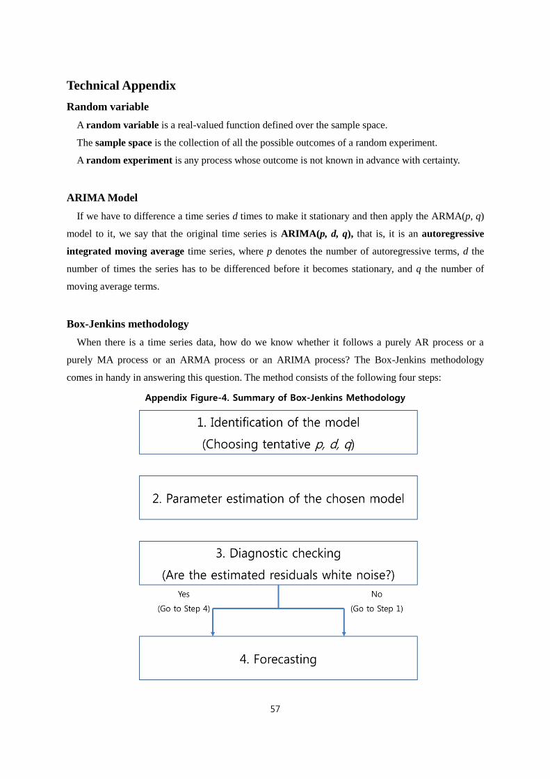
57

Technical Appendix

Random variable

A random variable is a real-valued function defined over the sample space.

The sample space is the collection of all the possible outcomes of a random experiment.

A random experiment is any process whose outcome is not known in advance with certainty.

ARIMA Model

If we have to difference a time series d times to make it stationary and then apply the ARMA(p, q)

model to it, we say that the original time series is ARIMA(p, d, q), that is, it is an autoregressive

integrated moving average time series, where p denotes the number of autoregressive terms, d the

number of times the series has to be differenced before it becomes stationary, and q the number of

moving average terms.

Box-Jenkins methodology

When there is a time series data, how do we know whether it follows a purely AR process or a

purely MA process or an ARMA process or an ARIMA process? The Box-Jenkins methodology

comes in handy in answering this question. The method consists of the following four steps:

Appendix Figure-4. Summary of Box-Jenkins Methodology

58

Spurious Regression

If there are two time series data which are nonstationary and not related with each other, the

regression of one variable on the other variable shows that there would be a statistically significant

relationship between these two variables. This is known as “spurious regression phenomenon”.

Maximum likelihood estimation

The method of maximum likelihood estimation will choose that value of the unknown parameter p

that maximizes the probability (likelihood) of randomly drawing the sample that was actually

obtained.

Test statistic

In statistical hypothesis testing, a hypothesis test is typically specified in terms of a test statistic,

which is a function of the sample; it is considered as a numerical summary of a set of data that

reduces the data to one or a small number of values that can be used to perform a hypothesis test.

59

Shipping Terminology118

Four Main Shipping Markets

Sea transport services are provided by four closely related markets, each trading in a different

commodity:

The freight market trades in sea transport service.

The sale and purchase market trades secondhand ships.

The newbuilding market trades new ships.

The demolition market deals in ships for scrapping.

By Ship Type

Basically, the ship can be a cargo ship or non-cargo ship. The cargo ships can be classified into the

four types as follows:

1) General cargo ship: Container ship, Ro-Ro, Barge carrier, Multi-purpose ship, Heavy lift,

Reefer ship, General cargo ship, etc.

2) Dry bulk ship: bulk carrier, ore carrier, vehicle carrier, cement carrier, etc.

3) Oil and chemicals ship: crude tanker, products tanker, chemical tanker, combined carrier, etc.

4) Liquid Gas ship: LPG ship, LNG ship, etc.

The ship which is considered in this report belongs to the type of dry bulk ship.

Deadweight Tonnage (DWT)

The deadweight tonnage of a ship measures the total weight of cargo that the vessel can carry when

loaded down to its marks, including the weight of fuel, stores, water ballast, fresh water, crew,

passengers, and baggage. So, it can represent the cargo-carrying capacity of a fleet of ships.

Size of Dry Bulk Ships by DWT and Their Main Commodities

Capesize: above 100,000 DWT, Panamax: 60,000~100,000 DWT,

Handymax: 40,000~60,000 DWT, Handysize: 10,000~40,000 DWT

- Iron Ore Coal Grain Bauxite &

Alumina

Phosphate

Rock

Capesize 70% 45% 7% - -

Panamax 22% 40% 43% 45% 20%

Handy 8% 15% 50% 55% 80%

118

This Chapter is mainly based on Stopford (2009), Alizadeh and Nomikos (2010) and Alizadeh and Nomikos

(2009).

60

Various Contract Types of Dry Bulk Freight Market

1) Voyage charter contract: Under this contract, the shipowner agrees to transport a specified

amount of cargo from a designated loading port to a designated discharging port in return for a

sum of money, known as ‘freight’. These contracts are also known as ‘spot contracts’ in the

shipping industry. The freight paid by the charterers (cargo owners) is normally expressed in

U.S. dollars per metric ton (US$/ton) of cargo or as a lump-sum. Shipowner is responsible for

the voyage cost.

2) Contracts of affreightment (CoA): This contract is that shipping contract under which the

shipowner agrees to transport specified amounts of cargo from the loading port or area to the

discharging port or region. This type of contract is normally used when the amount of cargo is

large and cannot be transported in a single shipment. The method and terms of payment in

CoAs is similar to voyage charter contract. Also, shipowner is responsible for the voyage cost.

3) Trip charter contract: This contract is a shipping contract under which the charterer agrees to

hire the vessel from the shipowner for the duration of a specified trip. Normally the charterer

takes charge of the vessel from the point of delivery to the point of redelivery (after

transportation of cargo) and pays the freight on a dollar-per-day basis (US$/day). The charterer

is responsible for the voyage cost. However, the shipowner has the operational control of the

vessel.

4) Time charter contract: Under this contract, the charterer agrees to hire the vessel from the

shipowner for a specified period of time (any period from a round trip to several years). The

freight rates are agreed on and paid on a US$/day basis. Under this contract, the charterer takes

the commercial control of the vessel, and benefits from operational flexibility as well as

security in transportation costs.

61

References

(1) Adland, R. and K. Cullinane (2006), “The Non-linear Dynamics of Spot Freight Rates in

Tanker Markets”, Transportation Research, Part E, 42, pp.211-224.

(2) Adland, R. and S. P. Strandenes (2007), “A Discrete-Time Stochastic Partial Equilibrium

Model of the Spot Freight Market”, Journal of Transport Economics and Policy, Vol. 41, Part 2,

pp.189-218.

(3) Alizadeh, A. H., R. O. Adland and S. Koekebakker (2007), “Predictive Power and

Unbiasedness of Implied Forward Charter Rates”, Journal of Forecasting 26, pp.385-403.

(4) Alizadeh, A. H. and N. Nomikos (2010), “An Overview of the Dry Bulk Shipping Industry”,

The Handbook of Maritime Economics and Business, edited by Grammenos, C. TH., pp.319-353.

(5) Alizadeh, A. H. and N. Nomikos (2009), Shipping Derivatives and Risk Management,

Palgrave Macmillan.

(6) Alizadeh, A. H. and N. Nomikos (2003), “Do FFAs provide good forecasts?”, Lloyd’s

Shipping Economist, December, pp.32-34.

(7) Alizadeh, A. H. and W. K. Talley (2011), “Microeconomic Determinants of Dry Bulk

Shipping Freight Rates and Contract Times”, Transportation 38, pp.561-579.

(8) Batchelor, R., A. Alizadeh and I. Visvikis (2007), “Forecasting Spot and Forward Prices in

the International Freight Market”, International Journal of Forecasting 23, pp.101-114.

(9) Beenstock, M (1985), “A Theory of Ship Prices”, Maritime Policy and Management, Vol. 12,

No. 3, pp.215-225.

(10) Beenstock, M. and A. Vergottis (1993a), Econometric Modelling of World Shipping,

Chapman & Hall.

(11) Beenstock, M. and A. Vergottis (1993b), “The Interdependence between the Dry Cargo

and Tanker Markets”, Logistics and Transportation Review, pp.3-38.

(12) Beenstock, M. and A. Vergottis (1989a), “An Econometric Model of the World Market for

Dry Cargo Freight and Shipping”, Applied Economics, 21, pp.339-356.

(13) Beenstock, M. and A. Vergottis (1989b), ”An Econometric Model of the World Tanker

Market”, Journal of Transport Economics and Policy, pp.263-280.

(14) Bierens, H. J. and L. F. Martins (2010), “Time-Varying Cointegration”, Econometric Theory,

26, pp.1453-1490.

(15) Brown, J. P., H. Song and A. McGillivray (1997), “Forecasting UK House Prices: A Time

Varying Coefficient Approach”, Economic Modelling 14, pp.529-548.

(16) Calvet, L., M. Gonzalez-Eiras and P. Sodini (2004), “Financial Innovation, Market

Participation and Asset Prices”, Journal of Financial and Quantitative Analysis 39(3), pp.431-459.

62

(17) Chang, C.-C., C.-Y. Hsieh and Y.-C. Lin (2012), “A Predictive Model of the Freight Rate of

the International Market in Capesize Dry Bulk Carriers”, Applied Economics Letters 19, pp.313-317.

(18) Chrystal, K. A. and P. D. Mizen (2001), “Goodhart’s Law: Its Origins, Meaning and

Implications for Monetary Policy”.

(19) Chung, K. and Y. Ha (2010a), “The Structural Change in the BDI Function Due to the

Global Financial Crisis: Using the Kalman Filter”, Journal of Shipping and Logistics, Vol. 65, pp.217-

231.

(20) Chung, K. and Y. Ha (2010b), “The Empirical Analysis for the Effect of Global Financial

Crisis to the Baltic Dry Index”, Journal of Shipping and Logistics, Vol. 64, pp.1-16.

(21) Clarkson (2011), Shipping Intelligence Weekly, 23 September

(22) Clements, M. P. and D. F. Hendry, eds. (2004), A Companion to Economic Forecasting,

Blackwell Publishing Ltd.

(23) Cogley, T. and T. J. Sargent (2005), “Drifts and Volatilities: Monetary Policies and

Outcomes in the Post WWⅡ US”, Review of Economic Dynamics 8, pp.262-302.

(24) Colander, D., ed. (2006), Post Walrasian Macroeconomics: Beyond the Dynamic Stochastic

General Equilibrium Model, Cambridge University Press.

(25) Covey, S. (1989), The Seven Habits of Highly Effective People, FranklinCovey Company.

(26) Dangl, T. and M. Halling (2011), “Predictive Regressions with Time-Varying Coefficients”,

Working Paper.

(27) De Mello, M. M. (2009), “The Role of Cointegration in the Forecast Accuracy of VAR

Models”, Working Paper.

(28) Dickey, D. and W. A. Fuller (1979), “Distribution of the Estimates for Autoregressive Time

Series with a Unit Root”, Journal of the American Statistical Association 74, pp.427-431.

(29) Diebold, F. X. (2006), Elements of Forecasting, Thomson South-Western.

(30) Diebold, F. X. (1998), “The Past, Present, and Future of Macroeconomic Forecasting”, The

Journal of Economic Perspectives, 2, pp.175-192.

(31) Diebold, F. X. and G. D. Rudebusch (1999), Business Cycles, Princeton University Press.

(32) Dikos G., H. Marcus, M. P. Papadatos and V. Papakonstantinou (2006), “Nivers Lines: A

System-Dynamics Approach to Tanker Freight Modeling”, Interface, Vol. 36, No. 4, pp.326-341.

(33) Elliot, G., C. W. J. Granger and A. Timmermann, eds. (2006), Handbook of Economic

Forecasting, Vol. 1, Elsevier B. V.

(34) Engelen S., W. Dullaert, B. Vernimmen (2009), “Market Efficiency within Dry Bulk

Markets in the Short Run: A Multi-Agent System Dynamics Nash Equilibrium”, Maritime Policy and

Management, Vol. 36, No. 5, pp.385-396.

63

(35) Engle, R. F. and C. W. J. Granger (1987), “Co-Integration and Error Correction:

Representation, Estimation, and Testing”, Econometrica, Vol. 55, No. 2, pp.251-276.

(36) Engle, R. and M. W. Watson (1987), “The Kalman Filter: Applications to Forecasting and

Rational-Expectations Models”, Advances in Econometrics, Fifth World Congress, edited by Bewley,

T., Cambridge University Press, pp.245-284.

(37) Fama, E. F. and G. W. Schwart (1977), “Asset Returns and Inflation”, Journal of Financial

Economics 5, pp.115-146.

(38) Garbade, K. and W. Silber (1993), “Price Movements and Price Discovery in Futures and

Cash Markets”, Review of Economics and Statistics 65, pp.289-297.

(39) Glen, D. R. (2006), “The Modelling of Dry Bulk and Tanker Markets: a Survey”, Maritime

Policy and Management, Vol. 33, No. 5, pp.431-445.

(40) Glen, D. R. (1997), “The Market for Second-hand Ships: Further Results on Efficiency

Using Cointegration Analysis”, Maritime Policy and Management, Vol. 24, No. 3, pp.245-260.

(41) Glosten, L. R., R. Jagannathan and D. Runkle, “On the Relation between the Expected Value

and the Volatility of the Nominal Excess Return on Stocks”, Journal of Finance 48, pp.1779-1801.

(42) Goodhart, C. A. E. (1975a), “Monetary Relationships: A View from Threadneedle Street” in

Papers in Monetary Economics, Vol. Ⅰ, Reserve Bank of Australia.

(43) Goodhart, C. A. E. (1975b), “Problems of Monetary Management: The UK Experience” in

Papers in Monetary Economics, Vol. Ⅰ, Reserve Bank of Australia.

(44) Goulielmos, A. M. and M. Psifia (2009), “Forecasting Weekly Freight Rates for One-Year

Time Charter 65 000 dwt Bulk Carrier, 1989-2008, using nonlinear methods”, Maritime Policy and

Management, Vol. 36, No. 5, pp.411-436.

(45) Goyal, A. and I. Welch (2003), “Predicting the Equity Premium with Dividend Ratios”,

Management Science 49, pp.639-654.

(46) Goyal, A. and I. Welch (2004), “A Comprehensive Look at the Empirical Performance of

Equity Premium Prediction”, NBER Working Paper 10483.

(47) Gratsos, G. A., H. A. Thanopoulou and A. W. Veenstra (2012), “Dry Bulk Shipping”, The

Blackwell Companion to Maritime Economics, edited by Talley, W. K., pp.187-204.

(48) Gujarati, D. N. (2003), Basic Econometrics, McGraw-Hill/Irwin.

(49) Hale, C. and A. Vanags (1992), “The Market for Second-hand Ships: Some Results on

Efficiency Using Cointegration”, Maritime Policy and Management, Vol. 19, No. 1, pp.31-39.

(50) Hamilton, J. D. (1994), Time Series Analysis, Princeton University Press.

(51) Heckman, J. J. (1976), “The Common Structure of Statistical Models of Truncation, Sample

Selection, and Limited Dependent Variables and a Simple Estimator for Such Models”, Annals of

Economic and Social Measurement 5, pp.475-492.

64

(52) Hjalmarsson, E. (2006), “Should We Expect Significant Out-of-Sample Results When

Predicting Stock Returns?”, International Finance Discussion Papers, No. 855, Board of Governors of

the Federal Reserve System.

(53) Hoover, K. D. (2006), “The Past as the Future: The Marshallian Approach to Post Walrasian

Econometrics”, Post Walrasian Macroeconomics: Beyond the Dynamic Stochastic General

Equilibrium Model, edited by Colander, D., Cambridge University Press, pp.239-257.

(54) Hoover, K. D., S. Johansen and K. Juselius (2008), “Allowing the Data to Speak Freely: The

Macroeconometrics of the Cointegrated Vector Autoregression”, American Economic Review: Papers

& Proceedings, 98:2, pp.251-255.

(55) Ibrahim, M. and W. J. Florkowski (2007), “Forecasting U.S. Shelled Pecan Prices: A

Cointegration Approach”, Selected Paper Prepared for Presentation at the Southern Agricultural

Economics Annual Meeting, Mobile, Alabama.

(56) Johansen, S. (1995), Likelihood-Based Inference in Cointegrated Vector Auto-Regressive

Models, Oxford University Press.

(57) Johansen, S. (1988), “Statistical Analysis of Cointegration Vectors”, Journal of Economic

Dynamics and Control 12, pp.231-254.

(58) Juselius, K. and S. Johansen (2006), “Extracting Information from the Data: A European

View on Empirical Macro”, Post Walrasian Macroeconomics: Beyond the Dynamic Stochastic

General Equilibrium Model, edited by Colander, D., Cambridge University Press, pp.239-257.

(59) Kaletsky, A. (2010), Captialism 4.0: The Birth of a New Economy in the Aftermath of Crisis,

PublicAffairs.

(60) Kavussanos, M. G. and N. K. Nomikos (2003), “Price Discovery, Causality and Forecasting

in the Freight Futures Market”, Review of Derivatives Research, 6, pp.203-230.

(61) Kavussanos, M. G. and I. D. Visvikis (2004), “Market Interactions in Returns and

Volatilities between Spot and Forward Shipping Freight Markets”, Journal of Banking & Finance 28,

pp.2015-2049.

(62) Kavussanos, M. G., I. D. Visvikis and R. A. Batchelor (2004), “Over-the-Counter Forward

Contracts and Spot Price Volatility in Shipping”, Transportation Research Part E 40, pp.273-296.

(63) Kavussanos, M. G., I. D. Visvikis and D. Menachof (2004), “The Unbiasedness Hypothesis

in the Freight Forward Market: Evidence from Cointegration Tests”, Review of Derivatives Research,

7, pp.241-266.

(64) Kim, C. –J., “Time Series Models” in Lecture Note on Econometrics, written by Whang, Y.

–J and C. –J. Kim, Korea University.

(65) Kim, C. –J. (2006), “Time-Varying Parameter Models with Endogenous Regressors”,

Economics Letters 91, pp.21-26.

65

(66) Kim, C. and C. Nelson (2006), “Estimation of a Forward-Looking Monetary Policy Rule: A

Time-Varying Parameter Model Using Ex Post Data”, Journal of Monetary Economics, 53, pp.1949-

1966.

(67) Kim, C. and C. Nelson (1999), State-Space Models with Regime Switching: Classical and

Gibbs-Sampling Approaches with Applications, The MIT Press.

(68) Ko, B. W. (2011a), “Dynamics of Dry Bulk Freight Market: Through the Lens of a Common

Stochastic Trend Model”, The Asian Journal of Shipping and Logistics, Vol. 27, No. 3, pp.387-404.

(69) Ko, B. W. (2011b), “An Application of Dynamic Factor Model to Dry Bulk Market -

Focusing on the Analysis of Synchronicity and Idiosyncrasy in the Sub-markets with Different Ship

Size -”, KMI International Journal of Maritime Affairs and Fisheries, Vol 3. Issue 1, pp.69-82.

(70) Ko, B. W. (2010), “A Mixed-Regime Model for Dry Bulk Freight Market”, The Asian

Journal of Shipping and Logistics, Vol. 26, No. 2, pp.185-204.

(71) Koop, G. and S. M. Potter (2011), “Time Varying VARs with Inequality Restrictions”,

Journal of Economic Dynamics & Control 35, pp.1126-1138.

(72) Koop, G., R. Leon-Gonzalez and R. W. Strachan (2011), “Bayesian Inference in a Time

Varying Cointegration Model”, Journal of Econometrics, 165, pp.210-220.

(73) Lettau, M. and S. Van Nieuwerburgh (2008), “Reconciling the Return Predictability

Evidence”, The Review of Financial Studies 21, pp.1607-1652.

(74) Li, J. and M. G. Parsons (1997), “Forecasting Tanker Freight Rate Using Neural Networks”,

Maritime Policy and Management, Vol. 24, No. 1, pp.9-30.

(75) Luo, M., L. Fan and L. Liu (2009), “An Econometric Analysis for Container Shipping

Market”, Maritime Policy and Management, Vol. 36, No. 6, pp.507-523.

(76) Lyridis, D., P. Zacharioudakis, P. Mitrou and A. Mylonas (2004), “Forecasting Tanker

Market Using Artificial Neural Networks”, Maritime Economics and Logistics, pp 93-108.

(77) Maritime Strategies International (2011), Dry Bulk Freight Forecaster November 2011.

(78) Obstfeld, M. and K. Rogoff (1996), Foundations of International Macroeconomics, The

MIT Press.

(79) Park, C. and C. –J. Kim (2009), “Time-Varying Cointegration Relationship between

Dividends and Stock Price”, Working Paper.

(80) Park, J. Y. and S. B. Hahn (1999), “Cointegrating Regressions with Time Varying

Coefficients”, Econometric Theory, Vol. 15, No. 5, pp.664-703.

(81) Pastor, L. and R. F. Stanbaugh (2009), “Predictive Systems: Living with Imperfect

Predictors”, The Journal of Finance, Vol. LXIV, No. 4, pp.1583-1628.

(82) Quantitative Micro Software, EViews 6 User’s Guide.

66

(83) Quintos, C. E. and P. C. B. Phillips (1993), “Parameter Constancy in Cointegrating

Regressions”, Cowles Foundation Paper 861, Empirical Economics, pp.675-706.

(84) Randers, J. and U. Goluke (2007), “Forecasting Turning Points in Shipping Freight Rates:

Lessons from 30 Years of Practical Effort”, System Dynamics Review, Vol. 23, No. 2/3, pp.253-284.

(85) Rifkin, Jeremy (2004), The European Dream: How Europe’s Vision of the Future Is Quietly

Eclipsing the American Dream.

(86) Rim, J., W. Kim. and B. Ko (2010), “An Empirical Analysis of the Dry Bulk Market Using a

Recursive VAR Model”, in Korean, Journal of Shipping and Logistics, Vol. 64, pp.17-35.

(87) Sims, C. A. (1993), “A Nine Variable Probabilistic Macroeconomic Forecasting Model”,

NBER Studies in Business: Business Cycles, Indicators, and Forecasting, Vol. 28, edited by Stock, J.

H. and M. W. Watson, University of Chicago Press, pp.179-212.

(88) Sims, C. A. (1980), “Macroeconomics and Reality”, Econometrica, Vol. 48, No. 1, pp.1-48.

(89) Stambaugh, R. F. (1999), “Predictive Regressions”, Journal of Financial Economics, 54,

pp.375-421.

(90) Stein, J. L. (1981), “The Simultaneous Determination of Spot and Futures Prices”, American

Economic Review, 51(5), pp.1012-1025

(91) Stock, J. H. and M. W. Watson (2001), “Vector Autoregressions”, Journal of Economic

Perspectives, Vol. 15, No. 4, pp.101-115

(92) Stopford, M. (2009), Maritime Economics, third edition, Routledge.

(93) Tashman, L. J. (2000), “Out-of-Sample Tests of Forecast Accuracy: An Analysis and

Review”, International Journal of Forecasting, 16, pp.437-450.

(94) The Baltic Exchange (2011), Manual for Panellists: A Guide to Freight Reporting and Index

Production.

(95) Tinbergen, J. (1934), “Scheepsruimte en vrachten”, De Nederlandsche Conjunctuur, March,

pp.23-35.

(96) Tinbergen, J. (1931), “Ein Schiffbauzyclus?”, Weltwirstschaftliches Archiv, 34, pp.152-164.

(97) Tvedt, J. (2003), “Shipping Market Models and the Specification of Freight Rate Processes”,

Maritime Economics and Logistics, pp.327-346.

(98) Tvedt, J. (2011), “Short-run Freight Rate Formation in the VLCC market: A Theoretical

Framework”, Maritime Economics and Logistics, Vol. 13, 4, pp.442-455.

(99) Veenstra, A. and J. van Dalen (2011), “Fixtures-based Freight Rate Indices, and their Impact

on Freight Rate Modelling in the Shipping Industry”, International Handbook of Maritime Economics

edited by Cullinane, K., Edward Elgar Publishing Limited, pp.63-84.

(100) Veenstra, A. W. and P. H. Franses (1997), “A Co-integration Approach to Forecasting

Freight Rates in the Dry Bulk Shipping Sector”, Transportation Research Part A: Policy and Practice,

67

Vol. 31, No. 6, pp.447-458.

(101) Waggoner, D. F. and T. Zha (1999), “Conditional Forecasts in Dynamic Multivariate

Models”, The Review of Economics and Statistics, Vol. 81, No. 4, pp.639-651.

(102) Watson, M. W. (1994), “Vector Autoregressions and Cointegression”, Handbook of

Econometrics, Vol. IV, edited by Engle, R. F. and D. L. McFadden, Elsevier Science, pp.2843-2915.

(103) Zhongzhen, Y., J. Lianjie and W. Minghua (2011), “Forecasting Baltic Panamax Index with

Support Vector Machine”, Journal of Transportation Systems Engineering and Information

Technology, Vol. 11, Issue 3, pp.50-57.

(104) Zuo, H. and S. Y. Park (2011), “Money Demand in China and Time-Varying

Cointegration”, China Economic Review 22, pp.330-343.

(105) http://www.clarkson.net

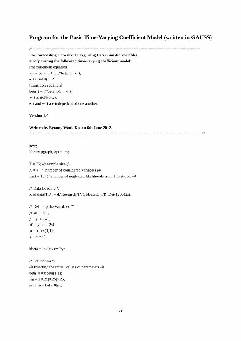
68

Program for the Basic Time-Varying Coefficient Model (written in GAUSS)

/* =========================================================================

For Forecasting Capesize TCavg using Deterministic Variables,

incorporating the following time-varying coefficient model:

[measurement equation]

y_t = beta_0 + x_t*beta_t + e_t,

e_t is iidN(0, R).

[transition equation]

beta_t = F*beta_t-1 + w_t,

w_t is iidN(o,Q),

e_t and w_t are indepedent of one another.

Version 1.0

Written by Byoung Wook Ko, on 6th June 2012.

=========================================================================== */

new;

library pgraph, optmum;

T = 75; @ sample size @

K = 4; @ number of considered variables @

start = 13; @ number of neglected likelihoods from 1 to start-1 @

/* Data Loading */

load data[T,K] = d:\Research\TVCI\Data\C_FR_Det(1206).txt;

/* Defining the Variables */

ymat = data;

y = ymat[.,1];

x0 = ymat[.,2:4];

xc = ones(T,1);

x = xc~x0;

bbeta = inv(x'x)*x'*y;

/* Estimation */

@ Inserting the initial values of parameters @

beta_0 = bbeta[1,1];

sig = 1|0.25|0.25|0.25;

prm_in = beta_0|sig;

69

@ run numercial optimization using the procedure, optmum @

{xout,fout,cout,gout} = optmum(&lnlik,prm_in);

@ Results @

prm_fn = trans(xout);

hess0 = hessp(&lnlik,xout);

cov = inv(hess0);

grd_fn = gradfd(&trans,xout);

cov_fn = grd_fn*cov*grd_fn';

se = sqrt(diag(cov_fn));

{predofy_BetaM} = filter(xout);

y_yhat_dist = predofy_BetaM[.,1:3];

BetaM = predofy_BetaM[.,4:6];

/* Showing the Results */

output file = d:\Research\TVCI\Data\prm_C_FR_Det(1206)_ver10.out reset;

prm_fn~se;

output off;

output file = d:\Research\TVCI\Data\y_yhat_dist_C_FR_Det(1206)_ver10.out reset;

y_yhat_dist;

output off;

output file = d:\Research\TVCI\Data\TCCoeff_C_FR_Det(1206)_ver10.out reset;

BetaM;

output off;

end;

@========================= end of Main Program =============================@

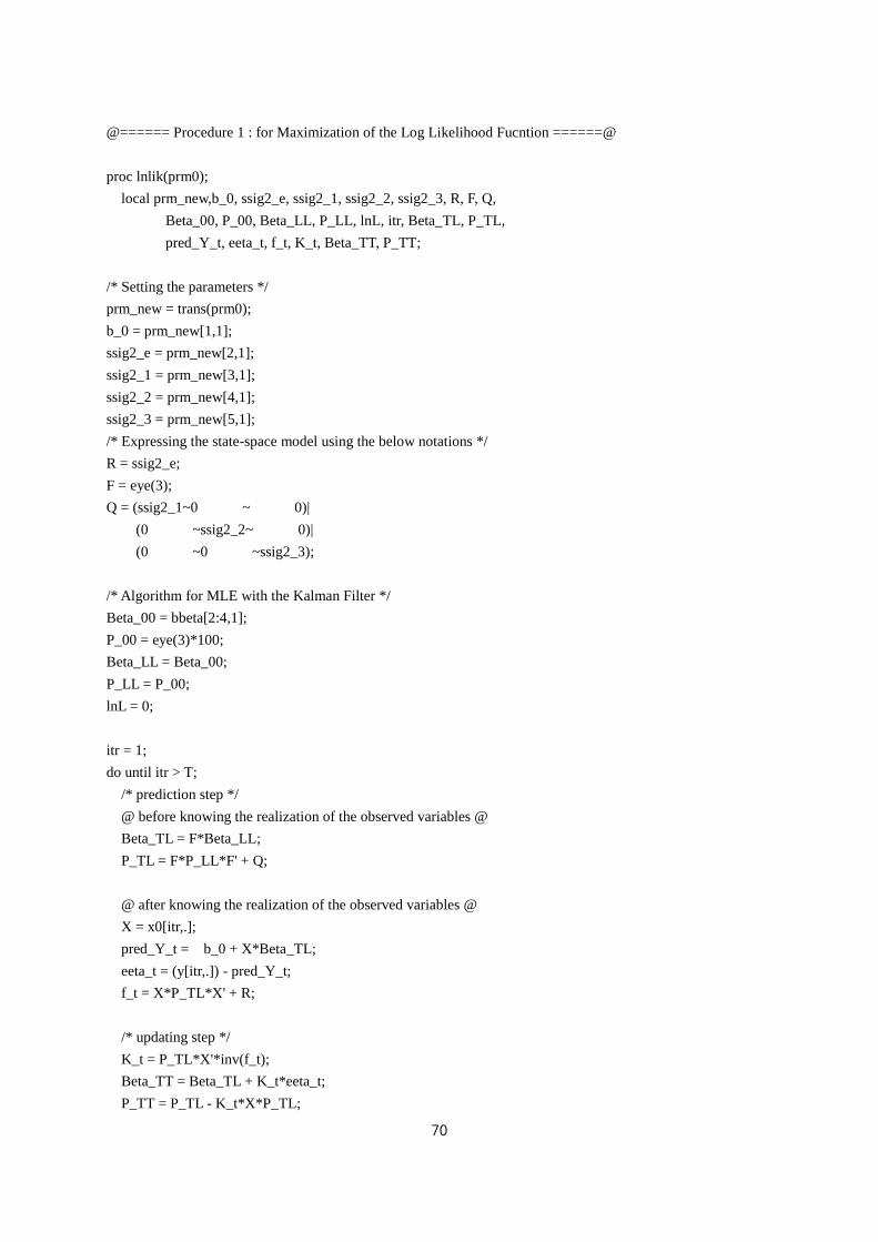
70

@====== Procedure 1 : for Maximization of the Log Likelihood Fucntion ======@

proc lnlik(prm0);

local prm_new,b_0, ssig2_e, ssig2_1, ssig2_2, ssig2_3, R, F, Q,

Beta_00, P_00, Beta_LL, P_LL, lnL, itr, Beta_TL, P_TL,

pred_Y_t, eeta_t, f_t, K_t, Beta_TT, P_TT;

/* Setting the parameters */

prm_new = trans(prm0);

b_0 = prm_new[1,1];

ssig2_e = prm_new[2,1];

ssig2_1 = prm_new[3,1];

ssig2_2 = prm_new[4,1];

ssig2_3 = prm_new[5,1];

/* Expressing the state-space model using the below notations */

R = ssig2_e;

F = eye(3);

Q = (ssig2_1~0 ~ 0)|

(0 ~ssig2_2~ 0)|

(0 ~0 ~ssig2_3);

/* Algorithm for MLE with the Kalman Filter */

Beta_00 = bbeta[2:4,1];

P_00 = eye(3)*100;

Beta_LL = Beta_00;

P_LL = P_00;

lnL = 0;

itr = 1;

do until itr > T;

/* prediction step */

@ before knowing the realization of the observed variables @

Beta_TL = F*Beta_LL;

P_TL = F*P_LL*F' + Q;

@ after knowing the realization of the observed variables @

X = x0[itr,.];

pred_Y_t = b_0 + X*Beta_TL;

eeta_t = (y[itr,.]) - pred_Y_t;

f_t = X*P_TL*X' + R;

/* updating step */

K_t = P_TL*X'*inv(f_t);

Beta_TT = Beta_TL + K_t*eeta_t;

P_TT = P_TL - K_t*X*P_TL;

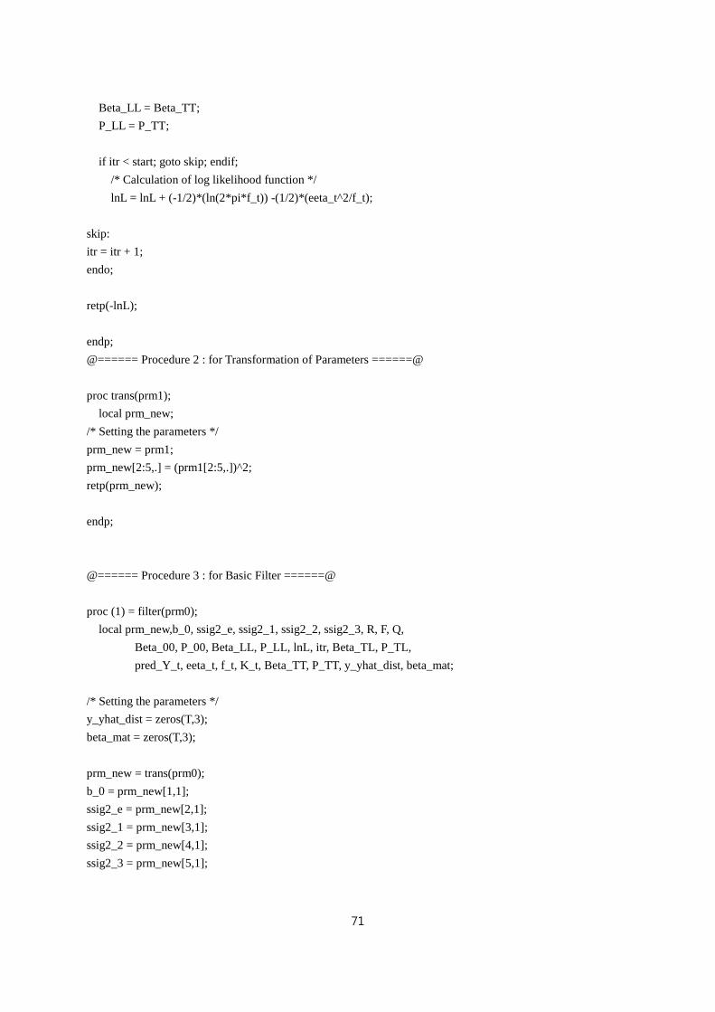
71

Beta_LL = Beta_TT;

P_LL = P_TT;

if itr < start; goto skip; endif;

/* Calculation of log likelihood function */

lnL = lnL + (-1/2)*(ln(2*pi*f_t)) -(1/2)*(eeta_t^2/f_t);

skip:

itr = itr + 1;

endo;

retp(-lnL);

endp;

@====== Procedure 2 : for Transformation of Parameters ======@

proc trans(prm1);

local prm_new;

/* Setting the parameters */

prm_new = prm1;

prm_new[2:5,.] = (prm1[2:5,.])^2;

retp(prm_new);

endp;

@====== Procedure 3 : for Basic Filter ======@

proc (1) = filter(prm0);

local prm_new,b_0, ssig2_e, ssig2_1, ssig2_2, ssig2_3, R, F, Q,

Beta_00, P_00, Beta_LL, P_LL, lnL, itr, Beta_TL, P_TL,

pred_Y_t, eeta_t, f_t, K_t, Beta_TT, P_TT, y_yhat_dist, beta_mat;

/* Setting the parameters */

y_yhat_dist = zeros(T,3);

beta_mat = zeros(T,3);

prm_new = trans(prm0);

b_0 = prm_new[1,1];

ssig2_e = prm_new[2,1];

ssig2_1 = prm_new[3,1];

ssig2_2 = prm_new[4,1];

ssig2_3 = prm_new[5,1];

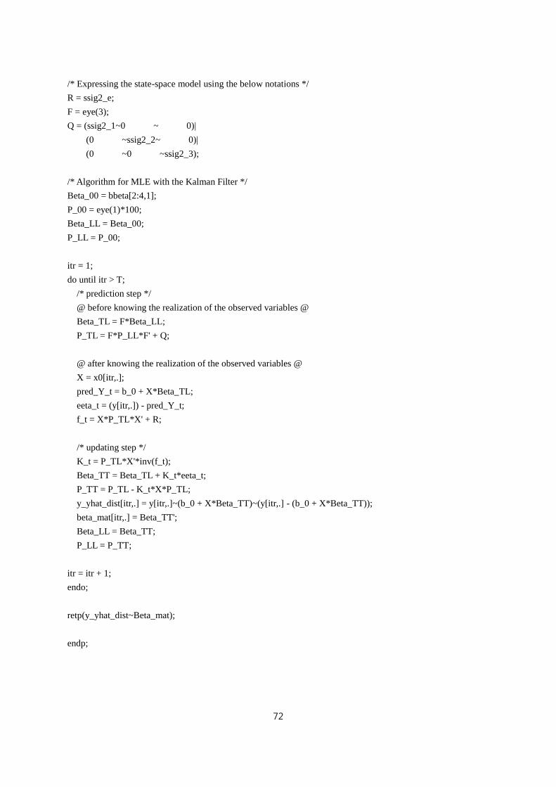
72

/* Expressing the state-space model using the below notations */

R = ssig2_e;

F = eye(3);

Q = (ssig2_1~0 ~ 0)|

(0 ~ssig2_2~ 0)|

(0 ~0 ~ssig2_3);

/* Algorithm for MLE with the Kalman Filter */

Beta_00 = bbeta[2:4,1];

P_00 = eye(1)*100;

Beta_LL = Beta_00;

P_LL = P_00;

itr = 1;

do until itr > T;

/* prediction step */

@ before knowing the realization of the observed variables @

Beta_TL = F*Beta_LL;

P_TL = F*P_LL*F' + Q;

@ after knowing the realization of the observed variables @

X = x0[itr,.];

pred_Y_t = b_0 + X*Beta_TL;

eeta_t = (y[itr,.]) - pred_Y_t;

f_t = X*P_TL*X' + R;

/* updating step */

K_t = P_TL*X'*inv(f_t);

Beta_TT = Beta_TL + K_t*eeta_t;

P_TT = P_TL - K_t*X*P_TL;

y_yhat_dist[itr,.] = y[itr,.]~(b_0 + X*Beta_TT)~(y[itr,.] - (b_0 + X*Beta_TT));

beta_mat[itr,.] = Beta_TT';

Beta_LL = Beta_TT;

P_LL = P_TT;

itr = itr + 1;

endo;

retp(y_yhat_dist~Beta_mat);

endp;

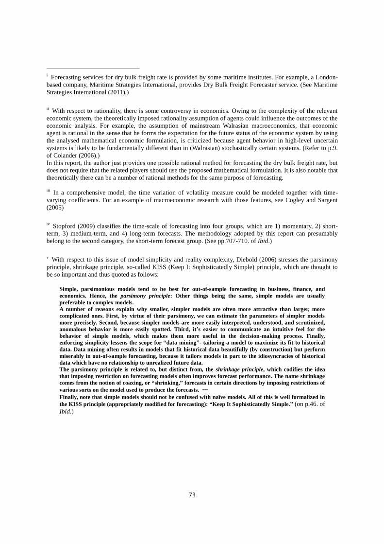
73

i Forecasting services for dry bulk freight rate is provided by some maritime institutes. For example, a London-

based company, Maritime Strategies International, provides Dry Bulk Freight Forecaster service. (See Maritime

Strategies International (2011).)

ii With respect to rationality, there is some controversy in economics. Owing to the complexity of the relevant

economic system, the theoretically imposed rationality assumption of agents could influence the outcomes of the

economic analysis. For example, the assumption of mainstream Walrasian macroeconomics, that economic

agent is rational in the sense that he forms the expectation for the future status of the economic system by using

the analysed mathematical economic formulation, is criticized because agent behavior in high-level uncertain

systems is likely to be fundamentally different than in (Walrasian) stochastically certain systems. (Refer to p.9.

of Colander (2006).)

In this report, the author just provides one possible rational method for forecasting the dry bulk freight rate, but

does not require that the related players should use the proposed mathematical formulation. It is also notable that

theoretically there can be a number of rational methods for the same purpose of forecasting.

iii

In a comprehensive model, the time variation of volatility measure could be modeled together with time-

varying coefficients. For an example of macroeconomic research with those features, see Cogley and Sargent

(2005)

iv Stopford (2009) classifies the time-scale of forecasting into four groups, which are 1) momentary, 2) short-

term, 3) medium-term, and 4) long-term forecasts. The methodology adopted by this report can presumably

belong to the second category, the short-term forecast group. (See pp.707-710. of Ibid.)

v With respect to this issue of model simplicity and reality complexity, Diebold (2006) stresses the parsimony

principle, shrinkage principle, so-called KISS (Keep It Sophisticatedly Simple) principle, which are thought to

be so important and thus quoted as follows:

Simple, parsimonious models tend to be best for out-of-sample forecasting in business, finance, and

economics. Hence, the parsimony principle: Other things being the same, simple models are usually

preferable to complex models.

A number of reasons explain why smaller, simpler models are often more attractive than larger, more

complicated ones. First, by virtue of their parsimony, we can estimate the parameters of simpler models

more precisely. Second, because simpler models are more easily interpreted, understood, and scrutinized,

anomalous behavior is more easily spotted. Third, it’s easier to communicate an intuitive feel for the

behavior of simple models, which makes them more useful in the decision-making process. Finally,

enforcing simplicity lessens the scope for “data mining”- tailoring a model to maximize its fit to historical

data. Data mining often results in models that fit historical data beautifully (by construction) but perform

miserably in out-of-sample forecasting, because it tailors models in part to the idiosyncracies of historical

data which have no relationship to unrealized future data.

The parsimony principle is related to, but distinct from, the shrinkage principle, which codifies the idea

that imposing restriction on forecasting models often improves forecast performance. The name shrinkage

comes from the notion of coaxing, or “shrinking,” forecasts in certain directions by imposing restrictions of

various sorts on the model used to produce the forecasts. …

Finally, note that simple models should not be confused with naïve models. All of this is well formalized in

the KISS principle (appropriately modified for forecasting): “Keep It Sophisticatedly Simple.” (on p.46. of

Ibid.)

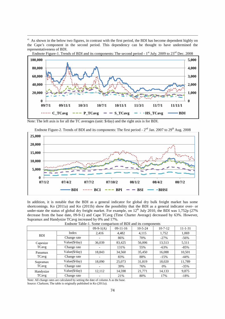
74

vi As shown in the below two figures, in contrast with the first period, the BDI has become dependent highly on

the Cape’s component in the second period. This dependency can be thought to have undermined the

representativeness of BDI.

Endnote Figure-1. Trends of BDI and its components: The second period - 1st July. 2009 to 23

rd Dec. 2008

Note: The left axis is for all the TC averages (unit: $/day) and the right axis is for BDI.

Endnote Figure-2. Trends of BDI and its components: The first period - 2nd

Jan. 2007 to 29th

Aug. 2008

In addition, it is notable that the BDI as a general indicator for global dry bulk freight market has some

shortcomings. Ko (2011a) and Ko (2011b) show the possibility that the BDI as a general indicator over- or

under-state the status of global dry freight market. For example, on 12th

July 2010, the BDI was 1,752p (27%

decrease from the base date, 09-9-1) and Cape TCavg (Time Charter Average) decreased by 63%. However,

Supramax and Handysize TCavg increased by 0% and 17%.

Endnote Table-1. Some comparison of BDI and its components

09-9-1(A) 09-11-16 10-5-24 10-7-12 11-1-31

BDI Index 2,416 4,482 4,115 1,752 1,069

Change rate - 86% 70% -27% -56%

Capesize

TCavg

Value($/day) 36,039 83,425 56,006 13,513 5,511

Change rate - 131% 55% -63% -85%

Panamax

TCavg

Value($/day) 18,843 34,560 35,450 16,088 10,501

Change rate - 83% 88% -15% -44%

Supramax

TCavg

Value($/day) 18,090 25,073 31,819 18,020 11,789

Change rate - 39% 76% 0% -35%

Handysize

TCavg

Value($/day) 12,112 14,598 21,771 14,133 9,875

Change rate - 21% 80% 17% -18%

Note: All change rates are calculated by setting the date of column A as the base. Source: Clarkson; The table is originally published in Ko (2011a).

0

1,000

2,000

3,000

4,000

5,000

0

20,000

40,000

60,000

80,000

100,000

09/7/1 09/11/1 10/3/1 10/7/1 10/11/1 11/3/1 11/7/1 11/11/1

C_TCavg P_TCavg S_TCavg HS_TCavg BDI

0

5,000

10,000

15,000

20,000

25,000

07/1/2 07/4/2 07/7/2 07/10/2 08/1/2 08/4/2 08/7/2

BDI BCI BPI BSI BHSI

75

vii

In recent literature on macroeconometrics there is some effort to re-identify the desirable relationship

between data and theory. For example, Hoover, Johansen and Juselius (2008) argue that obtaining good

characterizations of data before testing and drawing out the implications of data that ought to constrain

economic theorizing are important. For more discussion on this point, Hoover (2006) and Juselius and Johansen

(2006) are very helpful. Despite this importance of data analysis before rigorous derivation of theory, we must

have certain theory in mind explicitly or implicitly for the data analysis.

viii

The results of unit root test for the first-differenced value are as follows:

Endnote Table-2. Results of Unit Root Test for First-Differenced Value

- xt

None Constant

lnFR t-value -2.66 -2.67

p-value 0.008 0.08

lnCargo t-value -1.57 -2.36

p-value 0.10 0.15

lnShip t-value -0.83 -1.55

p-value 0.35 0.50

lnFFA t-value -2.75 -2.77

p-value 0.006 0.06

ix

For the nonstationarity of freight rates, Kavussanos and Nomikos (2003) insist that, becausse the relevant

demand variables and supply variables are both nonstationary, the freight rate determined by the interaction of

supply and demand should be nonstationary. (See p.212 of Ibid.)

x As shown in the below quote, Kaletsky (2010) insists that, in Capitalism 4.0 which is thought to be the new

regime after the 2008 global financial crisis, this kind of updating process will be right response to the uncertain

world.

If future is recognized as inherently unpredictable, paralysis is not the rational response to uncertainty.

The right response is for politicians and regulators, as well as investors and business leaders, to take

reasonable decisions on the information they have before them–and then be willing to modify or reverse

these decisions depending on how circumstances evolve. (On p.200. of Ibid.)

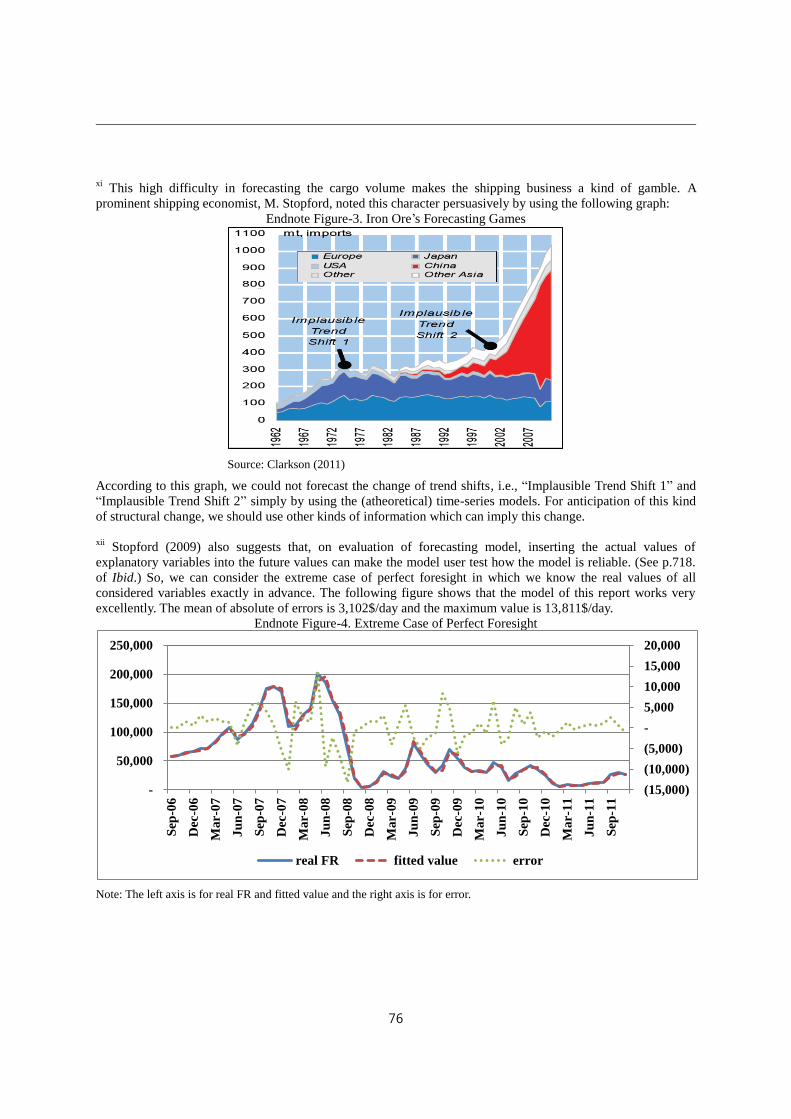
76

xi This high difficulty in forecasting the cargo volume makes the shipping business a kind of gamble. A

prominent shipping economist, M. Stopford, noted this character persuasively by using the following graph:

Endnote Figure-3. Iron Ore’s Forecasting Games

Source: Clarkson (2011)

According to this graph, we could not forecast the change of trend shifts, i.e., “Implausible Trend Shift 1” and

“Implausible Trend Shift 2” simply by using the (atheoretical) time-series models. For anticipation of this kind

of structural change, we should use other kinds of information which can imply this change.

xii

Stopford (2009) also suggests that, on evaluation of forecasting model, inserting the actual values of

explanatory variables into the future values can make the model user test how the model is reliable. (See p.718.

of Ibid.) So, we can consider the extreme case of perfect foresight in which we know the real values of all

considered variables exactly in advance. The following figure shows that the model of this report works very

excellently. The mean of absolute of errors is 3,102$/day and the maximum value is 13,811$/day.

Endnote Figure-4. Extreme Case of Perfect Foresight

Note: The left axis is for real FR and fitted value and the right axis is for error.

(15,000)

(10,000)

(5,000)

-

5,000

10,000

15,000

20,000

-

50,000

100,000

150,000

200,000

250,000

Sep

-06

Dec

-06

Mar-

07

Ju

n-0

7

Sep

-07

Dec

-07

Mar-

08

Ju

n-0

8

Sep

-08

Dec

-08

Mar-

09

Ju

n-0

9

Sep

-09

Dec

-09

Mar-

10

Ju

n-1

0

Sep

-10

Dec

-10

Mar-

11

Ju

n-1

1

Sep

-11

real FR fitted value error