a methodology for robust optimization of low-thrust trajectories in

A METHODOLOGY FOR ROBUST OPTIMIZATION OFLOW-THRUST TRAJECTORIES IN MULTI-BODY

ENVIRONMENTS

A ThesisPresented to

The Academic Faculty

by

Gregory Lantoine

In Partial Fulfillmentof the Requirements for the Degree

Doctor of Philosophy in theSchool of Aerospace Engineering

Georgia Institute of TechnologyDecember 2010

A METHODOLOGY FOR ROBUST OPTIMIZATION OFLOW-THRUST TRAJECTORIES IN MULTI-BODY

ENVIRONMENTS

Approved by:

Dr. Ryan P. Russell, AdvisorSchool of Aerospace EngineeringGeorgia Institute of Technology

Mr. Thierry DargentPlatform and Satellite Research GroupThales Alenia Space

Dr. Robert D. BraunSchool of Aerospace EngineeringGeorgia Institute of Technology

Dr. Jon A. SimsOuter Planets Mission Analysis GroupJet Propulsion Laboratory

Dr. John-Paul ClarkeSchool of Aerospace EngineeringGeorgia Institute of Technology

Dr. Panagiotis TsiotrasSchool of Aerospace EngineeringGeorgia Institute of Technology

Date Approved: 22 October 2010

To Linli

·��*�{

To my family

In commemoration of the Year of the Solar System

-ÞÃ/Ç�Y�e|

“Anything can be done with enough perseverance”

iii

ACKNOWLEDGEMENTS

This work would not have been possible without the support of many people over the

years. First, I would like to express my sincere gratitude and thanks to my advisor

Dr. Ryan Russell. It has been a privilege to work with you. Without your guidance,

wisdom, encouragement, and patience, this research would have not been possible.

Thank you for the invaluable scientific guidance and the contribution to many of the

ideas in this thesis. Your positiveness encouraged me and helped me in playing down

my worries and insecurities.

I am also extremely grateful to my old advisor, Dr. Robert Braun, who offered

me the possibility, back in 2007, to pursue a Ph.D. in the lab. Thank you for giving

me that opportunity and believing in me !

I shall also acknowledge Thales Alenia Space for funding part of this research. In

particular, it is difficult to know how to express my gratitude to Thierry Dargent.

This research simply would not have been possible without him. He was the impe-

tus behind this work, and he provided the support through Thales Alenia Space for

it to be completed. His willingness to invest a lot of time answering questions and

discussing research was very appreciated. Merci Thierry !

I am very grateful to each member of the Department of Aerospace Engineering

of Georgia Tech, because the environment has been friendly, supportive and stimu-

lating. Thank you also to my friends and labmates in the Space Systems Design Lab

and other labs. I really had a great time working with you. Especially I would like to

iv

thank Alexia Payan, Jarret Lafleur, Nitin Arora, Zarrin Chua, Brad Steinfeldt and

Mike Grant for being there for me so many times. With each one of you I have shared

unforgettable precious moments of my experience in Atlanta.

Furthemore, I would like to thank my family, who accepted my difficult decision

to come to Atlanta, and supported me every time, despite the distance. I would

especially like to thank my grand-parents for their unwavering support of me through

this process. And I would like to thank Laetitia for her wonderful encouragement and

support over these years.

Linli, living so far for all this time has been difficult. Thank you for your patience,

presence and love. I am incredibly fortunate to have you in my life. Tu es la seule et

unique.

Gregory Lantoine

October 2010

v

TABLE OF CONTENTS

DEDICATION . . . . . . . . . . . . . . . . . . . . . . . . . . . . . . . . . . . iii

ACKNOWLEDGEMENTS . . . . . . . . . . . . . . . . . . . . . . . . . . . . iv

LIST OF TABLES . . . . . . . . . . . . . . . . . . . . . . . . . . . . . . . . . xi

LIST OF FIGURES . . . . . . . . . . . . . . . . . . . . . . . . . . . . . . . . xiii

LIST OF SYMBOLS OR ABBREVIATIONS . . . . . . . . . . . . . . . . . . xviii

SUMMARY . . . . . . . . . . . . . . . . . . . . . . . . . . . . . . . . . . . . . xxi

I INTRODUCTION . . . . . . . . . . . . . . . . . . . . . . . . . . . . . . 1

1.1 Low-Thrust Propulsion . . . . . . . . . . . . . . . . . . . . . . . . . 2

1.2 Multi-Body Environment . . . . . . . . . . . . . . . . . . . . . . . 4

1.2.1 High-Energy, Two-Body Gravity-Assists . . . . . . . . . . . 5

1.2.2 Low-Energy, Three-Body Gravity-Assists . . . . . . . . . . . 5

1.3 Low-Thrust Trajectory Optimization . . . . . . . . . . . . . . . . . 7

1.4 Research Motivations and Objectives . . . . . . . . . . . . . . . . . 10

1.5 Organization of the Thesis . . . . . . . . . . . . . . . . . . . . . . . 14

1.6 Contributions . . . . . . . . . . . . . . . . . . . . . . . . . . . . . . 15

II UNIFIED OPTIMIZATION FRAMEWORK (OPTIFOR) . . . . . . . . 18

2.1 General Problem Formulation . . . . . . . . . . . . . . . . . . . . . 18

2.1.1 Direct Formulation . . . . . . . . . . . . . . . . . . . . . . . 20

2.1.2 Indirect Formulation . . . . . . . . . . . . . . . . . . . . . . 21

2.2 Implementation . . . . . . . . . . . . . . . . . . . . . . . . . . . . . 23

2.3 Interface with solvers . . . . . . . . . . . . . . . . . . . . . . . . . . 24

2.3.1 Supported solvers . . . . . . . . . . . . . . . . . . . . . . . . 24

2.3.2 Computation of sensitivities . . . . . . . . . . . . . . . . . . 25

III HDDP: AN HYBRID DIFFERENTIAL DYNAMIC PROGRAMMING AL-GORITHM FOR CONSTRAINED NONLINEAR OPTIMAL CONTROL

vi

PROBLEMS . . . . . . . . . . . . . . . . . . . . . . . . . . . . . . . . . 29

3.1 Introduction . . . . . . . . . . . . . . . . . . . . . . . . . . . . . . 29

3.1.1 Constrained Optimization . . . . . . . . . . . . . . . . . . . 36

3.1.2 Global Convergence . . . . . . . . . . . . . . . . . . . . . . 37

3.1.3 Independence between solver and user-supplied functions . . 38

3.1.4 Multi-phase capability . . . . . . . . . . . . . . . . . . . . . 38

3.2 Overview of DDP method . . . . . . . . . . . . . . . . . . . . . . . 40

3.2.1 Bellman Principle of Optimality . . . . . . . . . . . . . . . 40

3.2.2 Structure of the DDP Method . . . . . . . . . . . . . . . . . 41

3.3 The fundamental HDDP iteration . . . . . . . . . . . . . . . . . . . 43

3.3.1 Augmented Lagrangian Function . . . . . . . . . . . . . . . 43

3.3.2 STM-based Local Quadratic Expansions . . . . . . . . . . . 45

3.3.3 Minimization of constrained quadratic subproblems . . . . . 52

3.3.4 End of Iteration . . . . . . . . . . . . . . . . . . . . . . . . 66

3.4 Connection with Pontryagin Maximum Principle . . . . . . . . . . 71

3.5 Limitations of the algorithm . . . . . . . . . . . . . . . . . . . . . . 74

3.5.1 STM Computations . . . . . . . . . . . . . . . . . . . . . . 75

3.5.2 Tuning of the algorithm . . . . . . . . . . . . . . . . . . . . 75

3.6 Improvement of efficiency . . . . . . . . . . . . . . . . . . . . . . . 76

3.6.1 Parallelization of STM computations . . . . . . . . . . . . . 76

3.6.2 Adaptive mesh refinement . . . . . . . . . . . . . . . . . . . 76

3.6.3 Analytic State Transition Matrices . . . . . . . . . . . . . . 77

3.7 Validation of HDDP . . . . . . . . . . . . . . . . . . . . . . . . . . 77

3.8 Conclusion of this chapter . . . . . . . . . . . . . . . . . . . . . . . 78

IV MULTICOMPLEX METHOD FOR AUTOMATIC COMPUTATION OFHIGH-ORDER DERIVATIVES . . . . . . . . . . . . . . . . . . . . . . . 80

4.1 Introduction . . . . . . . . . . . . . . . . . . . . . . . . . . . . . . 80

4.2 Theory . . . . . . . . . . . . . . . . . . . . . . . . . . . . . . . . . 84

4.2.1 Definition of Multicomplex numbers . . . . . . . . . . . . . 84

vii

4.2.2 Holomorphic Functions . . . . . . . . . . . . . . . . . . . . 88

4.2.3 Multicomplex Step Differentiation . . . . . . . . . . . . . . 89

4.2.4 Simple Numerical Example . . . . . . . . . . . . . . . . . . 92

4.3 Implementation . . . . . . . . . . . . . . . . . . . . . . . . . . . . . 95

4.3.1 Implementation of multicomplex variables . . . . . . . . . . 95

4.3.2 Operator and Function Overloading . . . . . . . . . . . . . 97

4.3.3 Overall Procedure . . . . . . . . . . . . . . . . . . . . . . . 99

4.4 Applications . . . . . . . . . . . . . . . . . . . . . . . . . . . . . . 100

4.4.1 Simple Mathematical Function . . . . . . . . . . . . . . . . 101

4.4.2 Gravity Field Derivatives . . . . . . . . . . . . . . . . . . . 103

4.4.3 Trajectory State Transition Matrix . . . . . . . . . . . . . . 105

4.5 Conclusions of this chapter . . . . . . . . . . . . . . . . . . . . . . 108

V LOW-THRUST TRAJECTORY MODELS . . . . . . . . . . . . . . . . 110

5.1 Trajectory parameterization . . . . . . . . . . . . . . . . . . . . . . 110

5.2 Environment Models . . . . . . . . . . . . . . . . . . . . . . . . . . 111

5.2.1 Kepler Model . . . . . . . . . . . . . . . . . . . . . . . . . . 112

5.2.2 Stark Model . . . . . . . . . . . . . . . . . . . . . . . . . . 119

5.2.3 Constant Thrust Numerical Model . . . . . . . . . . . . . . 119

5.2.4 Impulsive Restricted Three-Body Model . . . . . . . . . . . 120

5.2.5 Indirect Two-Body Model . . . . . . . . . . . . . . . . . . . 120

5.3 Events . . . . . . . . . . . . . . . . . . . . . . . . . . . . . . . . . . 122

5.4 Objective functions . . . . . . . . . . . . . . . . . . . . . . . . . . . 123


VI THE STARK MODEL: AN EXACT, CLOSED-FORM APPROACH TOLOW-THRUST TRAJECTORY OPTIMIZATION . . . . . . . . . . . . 125

6.1 Introduction . . . . . . . . . . . . . . . . . . . . . . . . . . . . . . 125

6.2 Historical survey . . . . . . . . . . . . . . . . . . . . . . . . . . . . 129

6.3 Analysis of the planar Stark Problem . . . . . . . . . . . . . . . . . 134

6.3.1 Formulation of the planar problem . . . . . . . . . . . . . . 134

viii

6.3.2 Reduction to quadratures . . . . . . . . . . . . . . . . . . . 135

6.3.3 Integration of quadratures . . . . . . . . . . . . . . . . . . . 137

6.3.4 Summary and classification of the orbit solutions . . . . . . 150

6.3.5 Stark equation . . . . . . . . . . . . . . . . . . . . . . . . . 156

6.4 Analysis of the three-dimensional Stark problem . . . . . . . . . . . 159

6.4.1 Formulation of the problem . . . . . . . . . . . . . . . . . . 159

6.4.2 Reduction to quadratures . . . . . . . . . . . . . . . . . . . 160

6.4.3 Integration of quadratures . . . . . . . . . . . . . . . . . . . 161

6.4.4 Examples of three-dimensional Stark orbits . . . . . . . . . 167

6.4.5 Three-dimensional Stark equation . . . . . . . . . . . . . . . 172

6.5 Numerical Validation . . . . . . . . . . . . . . . . . . . . . . . . . . 173

6.6 Comparative Simulations of Low-Thrust Trajectories . . . . . . . . 175


VII NUMERICAL EXAMPLES . . . . . . . . . . . . . . . . . . . . . . . . . 182

7.1 Earth-Mars Rendezvous Transfer . . . . . . . . . . . . . . . . . . . 182

7.2 Multi-Revolution Orbital Transfer . . . . . . . . . . . . . . . . . . 187

7.3 GTOC4 Multi-Phase Optimization . . . . . . . . . . . . . . . . . . 191

7.4 GTOC5 Varying-Fidelity Optimization . . . . . . . . . . . . . . . . 195


VIII OPTIMIZATION OF LOW-ENERGY HALO-TO-HALO TRANSFERS BE-TWEEN PLANETARY MOONS . . . . . . . . . . . . . . . . . . . . . . 200

8.1 Introduction . . . . . . . . . . . . . . . . . . . . . . . . . . . . . . 202

8.2 Mechanism of Three-Body Resonant Gravity-AssistTransfers . . . . . . . . . . . . . . . . . . . . . . . . . . . . . . . . 207

8.3 Robust Initial Guess Generation . . . . . . . . . . . . . . . . . . . 211

8.3.1 Resonant Path Selection . . . . . . . . . . . . . . . . . . . . 212

8.3.2 Generation of Unstable Resonant Orbits . . . . . . . . . . . 223

8.3.3 Invariant Manifolds of Halo Orbits . . . . . . . . . . . . . . 225

8.3.4 Summary of the Initial Guess Procedure . . . . . . . . . . . 234

ix

8.4 Optimization Strategy . . . . . . . . . . . . . . . . . . . . . . . . . 235

8.4.1 Ideal Three-Body Optimizations . . . . . . . . . . . . . . . 236

8.4.2 End-to-End Patched Three-Body Optimization . . . . . . . 244

8.4.3 Higher-Fidelity, Ephemeris-Based Optimization . . . . . . . 245

8.5 Numerical results . . . . . . . . . . . . . . . . . . . . . . . . . . . . 247

8.5.1 Pure Resonance Hopping Transfers . . . . . . . . . . . . . . 247

8.5.2 Low-Thrust Resonance Hopping Transfer . . . . . . . . . . 252

8.5.3 Quasi-Ballistic Halo-to-Halo transfer . . . . . . . . . . . . . 253


IX CONCLUSIONS . . . . . . . . . . . . . . . . . . . . . . . . . . . . . . . 263

9.1 Dissertation Summary and Major Contributions . . . . . . . . . . . 263

9.2 Directions for Future work . . . . . . . . . . . . . . . . . . . . . . . 267

APPENDIX A RELATED PAPERS . . . . . . . . . . . . . . . . . . . . . 270

APPENDIX B PROOFS OF SOME MULTICOMPLEX PROPERTIES . . 272

APPENDIX C INTERACTIVE VISUALIZATION CAPABILITY . . . . . 274

APPENDIX D KICK FUNCTION AND APSE TRANSFORMATIONS INTHE CR3BP . . . . . . . . . . . . . . . . . . . . . . . . . . . . . . . . . 276

APPENDIX E RESONANT HOPPING TRANSFER DATA . . . . . . . . 278

REFERENCES . . . . . . . . . . . . . . . . . . . . . . . . . . . . . . . . . . . 281

VITA . . . . . . . . . . . . . . . . . . . . . . . . . . . . . . . . . . . . . . . . 303

x

LIST OF TABLES

1 Characteristics of typical propulsion systems. . . . . . . . . . . . . . . 2

2 Simple function example. . . . . . . . . . . . . . . . . . . . . . . . . . 102

3 Lunar gravitational potential example. . . . . . . . . . . . . . . . . . 104

4 Data of the trajectory propagation . . . . . . . . . . . . . . . . . . . 105

5 State transition matrix example for low-thrust spacecraft trajectory. . 107

6 Execution times of HDDP steps in Matlab for a representative problemusing 150 nodes. . . . . . . . . . . . . . . . . . . . . . . . . . . . . . . 117

7 Cases divided by the curves shown in boundary diagram of Figure 25. 151

8 Accuracy comparison between analytical and numerical integrationsfor the different two-dimensional and three-dimensional solutions ofthe Stark problem. . . . . . . . . . . . . . . . . . . . . . . . . . . . . 174

9 Data of the orbital transfer simulation. . . . . . . . . . . . . . . . . . 176

10 Speed and accuracy comparison (no perturbations considered). . . . . 177

11 Perturbations accuracy (relative to numerical integration). . . . . . . 178

12 Comparison of exact and approximated solutions (relative to numericalintegration). . . . . . . . . . . . . . . . . . . . . . . . . . . . . . . . . 180

13 Optimization results of the indirect smooting approach. SNOPT solveris used. . . . . . . . . . . . . . . . . . . . . . . . . . . . . . . . . . . . 184

14 Comparison of optimization results for the different models considered. 184

15 Comparison of results from different solvers. . . . . . . . . . . . . . . 186

16 Comparison of the Lagrange multipliers of the constraints. . . . . . . 186

17 Comparison results between HDDP and SNOPT for multi-rev transfers.188

18 Orbital Elements of the bodies encountered in the GTOC4 trajectory. 193

19 Optimal static parameters for each phase of the GTOC4 trajectory. . 193

20 Orbital Elements of the bodies encountered in the GTOC5 trajectory. 197

21 Optimal static parameters for each phase of the GTOC5 trajectory. . 197

22 Jupiter-Ganymede and Jupiter-Europa CR3BP parameters. . . . . . . 247

23 Description of the different transfers. . . . . . . . . . . . . . . . . . . 248

xi

24 Initial conditions (rotating frame) and characteristics of the Halo orbitsused in the transfer. Note y0 = 0, x0 = 0 and z0 = 0. . . . . . . . . . 254

25 Initial conditions and characteristics of the manifold trajectories shownin Figure 78. . . . . . . . . . . . . . . . . . . . . . . . . . . . . . . . . 254

26 Initial conditions (rotating frame) and characteristics of the periodicresonant orbits shown in Figure 78. Note y0 = 0, z0 = 0, x0 = 0 andz0 = 0. . . . . . . . . . . . . . . . . . . . . . . . . . . . . . . . . . . . 255

27 Optimization parameters of the two portions of the transfer. . . . . . 255

28 Initial conditions (inertial frame) in the generation of the ephemerismodel. . . . . . . . . . . . . . . . . . . . . . . . . . . . . . . . . . . . 256

29 Optimization Results for each model. . . . . . . . . . . . . . . . . . . 257

xii

LIST OF FIGURES

1 Overview of the low-thrust software prototype architecture. . . . . . . 13

2 Optimal Control Problem Structure with two phases. . . . . . . . . . 21

3 Sparsity Structure of the complete Jacobian given to NLP solvers. . . 27

4 Example of trajectory discretization with two phases. . . . . . . . . . 31

5 Optimal Control Problem Structure with two phases. . . . . . . . . . 35

6 Optimization flow of DDP. . . . . . . . . . . . . . . . . . . . . . . . . 42

7 Stage Structure. . . . . . . . . . . . . . . . . . . . . . . . . . . . . . . 46

8 Perturbation mapping. . . . . . . . . . . . . . . . . . . . . . . . . . . 48

9 Inter-Phase Structure. . . . . . . . . . . . . . . . . . . . . . . . . . . 49

10 Negative effect of bounds on trust region step estimations. . . . . . . 60

11 General procedure to generate required derivatives across the stages. . 63

12 Comparison of classical and STM-based discretization schemes. . . . . 74

13 Parallelization of STM computations. . . . . . . . . . . . . . . . . . . 76

14 Controls (left) and states (right) of the optimal solution. . . . . . . . 78

15 Normalized error: first-order derivative (left), second-order derivative(center), third-order derivative (right). Analytical estimate is the ref-erence. . . . . . . . . . . . . . . . . . . . . . . . . . . . . . . . . . . . 93

16 1st to 6th-order derivative relative errors . . . . . . . . . . . . . . . . 94

17 Tree Representation of a multicomplex number of order n. . . . . . . 96

18 Implemented Propagation Models. . . . . . . . . . . . . . . . . . . . . 111

19 Impulsive discretization scheme. . . . . . . . . . . . . . . . . . . . . . 113

20 Execution time contributions. . . . . . . . . . . . . . . . . . . . . . . 117

21 Representative plot of polynomial Pξ with two real positive roots. . . 139

22 Representative plot of polynomial Pξ with one real positive root. . . . 143

23 List of potential shapes of ξ solutions. Left : ξ1 solution. Center : ξ2and ξ3 solutions. Right : ξ4 and ξ5 solutions. . . . . . . . . . . . . . . 150

24 List of potential shapes of η solutions. Left : η1 solution. Right : η2solution. . . . . . . . . . . . . . . . . . . . . . . . . . . . . . . . . . . 150

xiii

25 Boundary diagram of the Stark problem. The domains of possiblemotion are denoted by the latin numbers. Markers give the location ofthe illustrative trajectories of figure 26 in the diagram. Square: ξ1η2solution. Circle: ξ2η2 solution. Diamond : ξ3η2 solution. Up triangle:ξ4η2 solution. Down triangle: ξ4η1 solution. Plus : ξ5η2 solution.Cross : ξ5η1 solution. . . . . . . . . . . . . . . . . . . . . . . . . . . . 152

26 Typical trajectories in the x − y plane of the Stark problem. Theconstant force is directed along the positive x-directionc. Dashed areascorrespond to forbidden regions. (a): ξ1η2 solution. (b): ξ2η2 solution.(c): ξ3η2 solution. (d): ξ4η2 solution. (e): ξ4η1 solution. (f): ξ5η2solution. (g): ξ5η1 solution. . . . . . . . . . . . . . . . . . . . . . . . 153

27 Typical evolution of a bounded trajectory. . . . . . . . . . . . . . . . 154

28 Representative plot of the Stark equation. . . . . . . . . . . . . . . . 158

29 Typical three-dimensional trajectories of the Stark problem. The con-stant force is directed along the positive z-direction. Gray areas corre-spond to the circular paraboloids that constrain the motion . . . . . . 168

30 Example of displaced circular orbit in the Stark problem (obtained byanalytical propagation). . . . . . . . . . . . . . . . . . . . . . . . . . 170

31 Evolution of an initially inclined circular orbit under the effect of avertical constant force. Parameters are X0 = [1, 0, 0, 0, 0.866, 0.5], µ =1, ε = 0.0103. The plot was obtained by analytical propagation fromsolution (ξI, η). . . . . . . . . . . . . . . . . . . . . . . . . . . . . . . 171

32 Evolution of semi-major axis, eccentricity, inclination and argument ofperiapsis. . . . . . . . . . . . . . . . . . . . . . . . . . . . . . . . . . 172

33 Trajectory of the orbital transfer. . . . . . . . . . . . . . . . . . . . . 176

34 Optimal Earth-Mars Rendezvous trajectory. . . . . . . . . . . . . . . 183

35 Thrust profiles for ε varying from 1 to 0. . . . . . . . . . . . . . . . . 183

36 Thrust profiles of the Earth-Mars trajectory using different models.(a): Constant Thrust Numerical Model (SNOPT). (b): AnalyticalStark Model (SNOPT). (c): Analytical Kepler Model (SNOPT). (d):Analytical Kepler Model (HDDP). . . . . . . . . . . . . . . . . . . . 185

37 Cost per iteration as a function of time of flight for HDDP and SNOPT.189

38 Trajectory of the case 4 transfer (from HDDP). . . . . . . . . . . . . 190

39 Thrust profile of case 4 from HDDP (left) and T3D (right). . . . . . . 190

xiv

40 Evolution of the constraints and associated Lagrange multipliers dur-ing optimization: semi-major axis constraint (left) and eccentricityconstraint (right). . . . . . . . . . . . . . . . . . . . . . . . . . . . . . 191

41 GTOC4 trajectory (Earth=blue, flybys=green, rendezvous=red): twodimensional top view (left) and three-dimensional view (right). . . . . 194

42 GTOC4 Thrust History (left) and Mass History (right). . . . . . . . . 194

43 Solution-finding process of our best GTOC5 trajectory. . . . . . . . . 196

44 GTOC5 trajectory (Earth=blue, flybys=green, rendezvous=red): two-dimensional top view (left) and three-dimensional view (right). . . . . 198

45 Phases of the GTOC5 trajectory. Each plot shows a rendezvous fol-lowed by a flyby of an asteroid. . . . . . . . . . . . . . . . . . . . . . 198

46 GTOC5 Thrust History (left) and Mass History (right). . . . . . . . . 199

47 Phases of Inter-Moon Resonant Gravity Assists. . . . . . . . . . . . . 208

48 Analytical kick function ∆a versus w at apoapsis, with a semi-majoraxis of a = 0.8618 and a Jacobi constant of C = 3.0024. . . . . . . . . 209

49 Effect of the flyby location w.r.t. moon. . . . . . . . . . . . . . . . . . 209

50 Structure of the initial guess. Ki : Li are resonant periodic orbits.Orbit figures are illustrative. . . . . . . . . . . . . . . . . . . . . . . . 212

51 Comparison of analytical and numerical kick function for an apoapsisflyby at Ganymede when the numerical integration is performed fromperiapsis to periapsis. . . . . . . . . . . . . . . . . . . . . . . . . . . . 215

52 Kick function for an apoapsis flyby at Ganymede. Left: Comparisonof analytical and numerical kick functions (numerical integration isperformed backwards and forwards from apoapsis). Right: Differencebetween analytical and numerical kick functions. . . . . . . . . . . . . 216

53 Time history of the semi-major axis (left) and the estimated Jacobiconstant C (right) across one flyby when Eq. (D.2) is used. . . . . . . 217

54 Minimum semi-major axis achievable as a function of number of mapapplications (i.e. orbits) for a0 = 0.86227 and C = 3.0058. . . . . . . 218

55 ∆a versus w0 obtained analytically and by integration for a0 = 0.86277(≈ 4:5 resonance) and 14 inertial revolutions in the Jupiter-Ganymedesystem. . . . . . . . . . . . . . . . . . . . . . . . . . . . . . . . . . . . 219

56 Time history of semi-major axis for the global minimum of Figure 55(found from the Keplerian Map). . . . . . . . . . . . . . . . . . . . . 219

57 Phase space generated using the Keplerian Map. . . . . . . . . . . . . 221

xv

58 Transport mechanism in the phase space of the three-body problem. . 221

59 3 : 4 resonant periodic orbit family at Ganymede (µ = 7.803710−5). . 224

60 Characteristics of the 3 : 4 family of resonant periodic orbits at Ganymede.224

61 Parameterization of trajectories along a manifold. . . . . . . . . . . . 228

62 Integration of the manifold to the first x-crossing. . . . . . . . . . . . 229

63 Semi-major axis Contour Map: C = 3.0069 (left) and C = 3.0059 (right).230

64 Successive manifold trajectories along an iso-line of the left contourmap of Figure 63 . . . . . . . . . . . . . . . . . . . . . . . . . . . . . 231

65 Successive manifold trajectories along a constant-ε line of the left con-tour map of Figure 63 . . . . . . . . . . . . . . . . . . . . . . . . . . 231

66 Evolution of the parameter α as a function of the Jacobi Constant C. 232

67 Comparison of semi-major axis values obtained from empirical andnumerical computations. . . . . . . . . . . . . . . . . . . . . . . . . . 233

68 Type I (left) and type II (right) manifold trajectories reaching the 4:5resonance (C = 3.0069). . . . . . . . . . . . . . . . . . . . . . . . . . 234

69 Formulation of the transfer problem. . . . . . . . . . . . . . . . . . . 238

70 Forward-Backward Multiple Shooting Setup (shown in rotating frames).239

71 Patch Point on the T-P Graph. . . . . . . . . . . . . . . . . . . . . . 243

72 Trajectory Scatter Plot for Ganymede-Europa transfer. . . . . . . . . 248

73 Quasi-ballistic Ganymede-Europa transfer in the inertial reference frame.250

74 Periapsis, apoapsis, and semi-major axis time evolution of the quasi-ballistic transfer. . . . . . . . . . . . . . . . . . . . . . . . . . . . . . 250

75 Ganymede portion of the quasi-ballistic transfer in the rotating refer-ence frame of Ganymede (left). Europa portion of the quasi-ballistictransfer in the rotating reference frame of Europa (right). . . . . . . . 251

76 Left: T-P graph of the quasi-ballistic transfer. Right: Zoom of theT-P graph on the switching region. . . . . . . . . . . . . . . . . . . . 252

77 Inertial trajectory (left) and thrust profile (right) of the low-thrust,low-energy transfer. . . . . . . . . . . . . . . . . . . . . . . . . . . . . 253

78 Orbits composing the initial guess of the transfer (rotating frames). . 254

79 Comparisons between the CR3BP and four-body ephemeris models.Left: difference in Ganymede and Europa orbital radii. Right: Jupiterpositions in the two models. . . . . . . . . . . . . . . . . . . . . . . . 256

xvi

80 Trajectory from Ganymede to Europa in inertial frame (patched CR3BPmodel). . . . . . . . . . . . . . . . . . . . . . . . . . . . . . . . . . . 258

81 Time history of semi-major axis, periapsis and apoapsis of the trajec-tory (patched CR3BP model). . . . . . . . . . . . . . . . . . . . . . . 258

82 Left: Ganymede-dominant phase in rotating frame. Right: Zoom inon Ganymede flybys. . . . . . . . . . . . . . . . . . . . . . . . . . . . 259

83 Left: Europa-dominant phase in rotating frame. Right: Zoom in onEuropa flybys. . . . . . . . . . . . . . . . . . . . . . . . . . . . . . . . 259

84 Trajectory from Ganymede to Europa in inertial frame (ephemerismodel). . . . . . . . . . . . . . . . . . . . . . . . . . . . . . . . . . . 260

85 Left: Time history of impulses (ephemeris model). Right: Time historyof semi-major axis, periapsis and apoapsis of the trajectory (ephemerismodel). . . . . . . . . . . . . . . . . . . . . . . . . . . . . . . . . . . 260

86 Improvements from the developed techniques of the thesis. . . . . . . 266

87 VISFOR architecture. . . . . . . . . . . . . . . . . . . . . . . . . . . 275

88 VISFOR screenshot. . . . . . . . . . . . . . . . . . . . . . . . . . . . 275

xvii

LIST OF SYMBOLS OR ABBREVIATIONS

Acronyms

EP Electrical Propulsion

SEP Solar Electrical Propulsion

NEP Nuclear Electrical Propulsion

ESA European Space Agency

NASA National Aeronautics and Space Administration

JPL Jet Propulsion Laboratory

JIMO Jupiter Icy Moons Mission

EJSM Europa Jupiter System Mission

JEO Jupiter Europa Orbiter

JGO Jupiter Ganymede Orbiter

LTGA Low-Thrust Gravity Assist

CR3BP Circular Restricted Three-Body Problem

OPTIFOR Optimization in Fortran

VISFOR Visual Interactive Simulation in Fortran

DDP Differential Dynamic Programming

HDDP Hybrid Differential Dynamic Programming

NLP Non-Linear Programming

STM State Transition Matrix

QP Quadratic Programming

SQP Sequential Quadratic Programming

AD Automatic Differentiation

MCX Multicomplex Differentiation

xviii

TOF Time of Flight

VILM Vinfinity Leveraging Maneuvers

DSM Deep Space Maneuver

CR3BP Circular Restricted Three-Body Problem

Symbols

T Thrust

Tmax Maximum Thrust

Isp Specific Impulse

x State vector: x ∈ <nx

X Augmented State vector: X ∈ <nx+nu+nw

u Dynamic Control vector: u ∈ <nu

w Static Control vector: w ∈ <nw

λ Lagrange multiplier

Γ Initial Function

F Transition Function

f Dynamical Function

L Stage Cost Function

φ Phase Cost Function

g Stage constraints

ψ Phase constraints

M Number of phases

N Number of stages

H Hamiltonian

S Switching Function

J Cost-to-go Function

∆ Trust Region Radius / Discriminant

D Scaling Matrix

xix

γ Shifting parameter

ER Expected Reduction

σ Penalty parameter

t Time variable

r Position

v Velocity

V∞ Relative Velocity

m Mass

ξ First Parabolic coordinate

η Second Parabolic coordinate

τ Fictitious Time

C Jacobi Constant

a Semi-major axis

e Eccentricity

ra Apoapsis

rp Periapsis

xx

SUMMARY

Future ambitious solar system exploration missions are likely to require ever larger

propulsion capabilities and involve innovative interplanetary trajectories in order to

accommodate the increasingly complex mission scenarios. Two recent advances in

trajectory design can be exploited to meet those new requirements: the use of low-

thrust propulsion which enables larger cumulative momentum exchange relative to

chemical propulsion; and the consideration of low-energy transfers relying on full

multi-body dynamics. Yet the resulting optimal control problems are hypersensitive,

time-consuming and extremely difficult to tackle with current optimization tools.

Therefore, the goal of the thesis is to develop a methodology that facilitates and

simplifies the solution finding process of low-thrust optimization problems in multi-

body environments. Emphasis is placed on robust techniques to produce good solu-

tions for a wide range of cases despite the strong nonlinearities of the problems. The

complete trajectory is broken down into different component phases, which facilitates

the modeling of the effects of multiple bodies and makes the process less sensitive to

the initial guess.

A unified optimization framework is created to solve the resulting multi-phase

optimal control problems. Interfaces to state-of-the-art solvers SNOPT and IPOPT

are included. In addition, a new, robust Hybrid Differential Dynamic Programming

(HDDP) algorithm is developed. HDDP is based on differential dynamic program-

ming, a proven robust second-order technique that relies on Bellman’s Principle of

xxi

Optimality and successive minimization of quadratic approximations. HDDP also

incorporates nonlinear mathematical programming techniques to increase efficiency,

and decouples the optimization from the dynamics using first- and second-order state

transition matrices.

Crucial to this optimization procedure is the generation of the sensitivities with

respect to the variables of the system. In the context of trajectory optimization, these

derivatives are often tedious and cumbersome to estimate analytically, especially when

complex multi-body dynamics are considered. To produce a solution with minimal

effort, an new approach is derived that computes automatically first- and high-order

derivatives via multicomplex numbers.

Another important aspect of the methodology is the representation of low-thrust

trajectories by different dynamical models with varying degrees of fidelity. Emphasis

is given on analytical expressions to speed up the optimization process. In particular,

one novelty of the framework is the derivation and implementation of analytic ex-

pressions for motion subjected to Newtonian gravitation plus an additional constant

inertial force.

Example applications include low-thrust asteroid tour design, multiple flyby tra-

jectories, and planetary inter-moon transfers. In the latter case, we generate good

initial guesses using dynamical systems theory to exploit the chaotic nature of these

multi-body systems. The developed optimization framework is then used to generate

low-energy, inter-moon trajectories with multiple resonant gravity assists.

xxii

Resume (Summary in French)

Les futures missions ambitieuses d’exploration du systeme solaire vont probable-

ment avoir besoin de capacites de propulsion de plus en plus importantes et incorporer

des trajectoires interplanetaires innovantes afin de tenir compte de scenarios de mis-

sions de plus en plus complexes. Deux avancees recentes dans la conception de trajec-

toires peuvent etre exploitees afin de repondre a ces nouvelles exigences: l’utilisation

de la propulsion a poussee faible qui permet d’accumuler de plus grands echanges

d’energie par rapport a la propulsion chimique; et la prise en compte des transferts

de faible energie s’appuyant sur la veritable dynamique multi-corps. Cependant,

les problemes correspondants de controle optimal sont hypersensibles, gourmands en

temps de calcul, et tres difficile a traiter avec les outils d’optimisation actuels.

Par consequent, l’objectif de cette these est de developper une methodologie qui

facilite et simplifie la recherche de solutions des problemes d’optimisation a poussee

faible dans des environnements multi-corps. L’accent est mis sur des techniques ro-

bustes permettant de produire de bonnes solutions pour un large eventail de cas,

malgre les fortes non-linearites des problemes. La trajectoire complete se decompose

en differentes phases, qui facilite la modelisation des effets des corps multiples et rend

le processus moins sensible a la solution initiale.

Un cadre unifie d’optimisation est cree pour resoudre le probleme multi-phase de

controle optimal ainsi obtenu. Des interfaces avec les solveurs recents SNOPT et

IPOPT sont incluses. En outre, un nouveau solveur (HDDP) est developpe. Celui-

ci est base sur la programmation dynamique differentielle, une technique robuste et

eprouvee de second ordre qui repose sur le principe d’optimalite de Bellman et la min-

imisation d’approximations quadratiques successives. HDDP integre egalement des

techniques de programmation mathematique non lineaires pour accroıtre l’efficacite,

xxiii

et decouple l’optimisation de la dynamique a l’aide des matrices de transition de pre-

mier et second ordres.

Un aspect crucial de cette procedure d’optimisation est la generation des sensi-

tivites par rapport aux variables du systeme. Dans le cadre de l’optimisation de tra-

jectoire, les derivees sont souvent laborieuses et complexes a estimer analytiquement,

en particulier lorsqu’une dynamique complexe multi-corps est prise en consideration.

Pour produire une solution avec un minimum d’effort, une nouvelle approche utilisant

les nombres multicomplexes est trouvee pour calculer automatiquement les derivees

premieres et d’ordres superieurs.

Un autre aspect important de la methodologie est la representation des trajectoires

a pousee faible par des modeles dynamiques de differents degres de fidelite. L’accent

est mis sur des expressions analytiques pour accelerer le processus d’optimisation. En

particulier, une nouveaute de la methodologie est la derivation et la mise en oeuvre

d’expressions analytiques dans le cas d’un mouvement soumis a la gravitation new-

tonienne et une force constante inertielle supplementaire.

Des exemples d’application sont donnes, comprenant des tours d’asteroıdes, des

trajectoires avec multiples flybys, ainsi que des transferts inter-lunes. Dans ce dernier

cas, une bonne estimation de la solution initiale est generee en utilisant la theorie

des systemes dynamiques afin d’exploiter la nature chaotique des systemes multi-

corps. La methodologie d’optimisation developpee est ensuite utilisee pour generer des

trajectoires de faible energie entre deux lunes grace a des assistances gravitationnelles

resonantes.

xxiv

CHAPTER I

INTRODUCTION

Interplanetary space travel has played an important role in the development of our

knowledge of the solar system. For decades, probes have been sent in various destina-

tions of the solar system to explore the unknown. This interest is still strong nowadays

as we expect an unprecedented number of planetary encounters and launches in the

coming years.64 In order to accommodate the increasingly complex mission scenarios,

future ambitious exploration missions are likely to involve innovative spacecraft tra-

jectories. In recent years, two developing concepts have been considered to reduce the

required propellant mass for interplanetary and intermoon missions, thus allowing for

increased mass of scientific payloads. Firstly, one significant capability is low-thrust

propulsion that allows for greatly improved fuel efficiency. This technology has there-

fore the potential to increase payload mass fractions as well as providing trajectories

not possible with impulsive thrust. Secondly, much attention is being focused on

taking advantage of the natural multi-body dynamics encountered in space, leading

to unconventional fuel-efficient trajectories. The robust optimization of the resulting

trajectories is therefore a key issue for the design of future missions. This thesis will

respond to this requirement and will develop methodologies to allow robust optimiza-

tion of low-thrust trajectories in multi-body environment.

This chapter introduces low-thrust trajectories and their optimal design in multi-

body environment. First, a brief overview of low-thrust propulsion is given. In this

context, the most relevant past, present and future missions that use this technology

are described. Subsequently, we present the classic and modern strategies to exploit

1

the gravity of multiple bodies in low-thrust missions. This is followed by a summary

of the current state-of-the-art in low-thrust trajectory optimization. Finally, the

motivations and objectives of this work are presented.

1.1 Low-Thrust Propulsion

Several propulsion systems have been developed to perform the velocity increments

required in space missions. These different propulsive options can be characterized

by the amount of thrust T they can produce and by the specific impulse Isp they can

achieve (see Table 1). The specific impulse measures the efficiency of propellant usage

since it is a measure of the amount of thrust that can be generated over a specified

time span per unit mass of fuel.

Table 1: Characteristics of typical propulsion systems.

Propulsion System Thrust (N) Isp (s)Cold Gas 0.05− 200 50− 250Chemical 0.1− 106 140− 460Electrical 10−5 − 5 150− 8000Solar Sail 0.001− 0.1 ∞

In the literature, the expression “low thrust” can encompass a broad variety of

quite different propulsion concepts, from solar sail to cold gas techniques. In this

thesis, low-thrust propulsion refers to electrical propulsion (EP) only. In contrast

to conventional ‘high-thrust’ trajectories that have thrust to coast ratios << 1, ‘low-

thrust’ trajectories generally are characterized thrust periods that occupy a significant

portion of the flight time. This low-thrust technology uses electrical energy to acceler-

ate the propellant. EP therefore provides much lower thrust levels than conventional

chemical propulsion does, but much higher specific impulse. It follows that an EP

engine device must thrust for a longer period to produce a desired change in trajec-

tory or velocity; however, the higher specific impulse enables a spacecraft using this

2

propulsion system to carry out a mission with relatively little propellant. The source

of the electrical energy for EP is independent of the propellant itself and may be so-

lar (solar electric propulsion, or SEP) or nuclear (nuclear electric propulsion, or NEP).

The attractiveness of EP for space missions was recognized by the patriarch of

modern rocketry, Robert H. Goddard, as early as 1906.96 However, the interest in

EP really started in the 60’s239 and since then a wide variety of EP devices have

been studied and developed. A comprehensive historical survey on the different EP

engines is given in Ref. 153 and Ref. 52. The first spacecraft to successfully use an EP

thruster for primary propulsion on an extended space mission was Deep Space 1 in

1998.204 In fact, one of the objectives of this mission was to test this new technology.

Similarly, ESA launched in 2003 its own test bed mission, known as Smart 1, to use

an EP thruster to get into orbit around the moon.200 Later on that year, Japan’s

Hayabusa spacecraft used electrical propulsion to embark on an asteroid sample re-

turn mission.249 The current Dawn mission,203 launched in 2007, is using EP to reach

asteroids Ceres and Vesta. Its accumulated thrust time is about 6 years, which would

not be feasible with chemical propulsion. At the time of this writing, the Dawn mis-

sion holds the all time record for most expended ∆V during the course of a space

mission.

Having proven itself to be an effective and reliable engine for primary propulsion,

the electrical thruster is now regularly considered in a variety of missions under devel-

opment.265 For instance, the incoming ESA mission BepiColombo to planet Mercury

(launch scheduled on 2013) will use both chemical and SEP systems.175 NEP was also

envisioned as the primary propulsion system for the now cancelled NASA’s Jupiter

Icy Moons Mission (JIMO).228 The main targets were Europa and Ganymede, which

are suspected to have liquid oceans beneath their surfaces. The JIMO is replaced

3

by the joint NASA/ESA Europa Jupiter System Mission to Jupiter’s moons, but the

new mission is expected to use classical chemical propulsion.2 Note that in the lat-

ter two missions, the multi-body effects play a crucial role: BepiColomo combines

low-thrust propulsion with gravity-assists to approach Mercury, and any Jupiter tour

missions must consider the gravitational forces of multiple moons. The effect of this

multi-body environment is the subject of the next section.

1.2 Multi-Body Environment

In the solar system, any spacecraft is inherently under the gravitational effects of the

Sun, the planets, the moons and other minor bodies. However, in most instances,

only one primary body can be regarded as dominant. The gravitational effects of

other bodies are then treated as mere perturbations. In this approach, the whole

velocity change required to accomplish the mission is provided only by the propulsion

system. To reduce fuel consumption, an improved method considers and exploits the

gravity of multiple bodies through gravity-assist maneuvers.

A gravity assist maneuver (or swing-by, or gravitational slingshot), is the use of

the gravity field of a planet or other massive celestial body to change the velocity of

a spacecraft as it passes close to this body162 . Due to this close encounter, there is

a momentum exchange between the spacecraft and the body, so that the spacecraft

increases or decreases its inertial velocity. Swing-bys therefore provide the capability

to modify, sometimes significantly, the trajectory without expending fuel.

In this thesis, we focus on the consideration of the multi-body environment to

design efficient low-thrust gravity assist (LTGA) trajectories. At this point, it is

convenient to distinguish two cases depending on the magnitude of velocity of the

spacecraft with respect to the flyby body. This separation fits with the historical

4

development of gravity-assist techniques.

1.2.1 High-Energy, Two-Body Gravity-Assists

First, when the relative velocity of the spacecraft is high during the gravity-assist, the

spacecraft undergoes a rapid crossing of the spheres of gravitational influencea of the

different bodies. In this first approximation, the spacecraft orbit is therefore deter-

mined by considering only one gravitational attraction at a time. This approximation

is reasonable because the duration of time when accelerations from both bodies are

comparable is very short.14 This classical design method is called the patched conic

approximation (or patched two-body approximation). NASA’s spectacular multiple

flyby missions such as Voyager125 and Galileo72 are based on this two-body decom-

position. As early as the 1970’s, the use of electric propulsion in conjunction with

gravity-assists was investigated to provide high-energy capability.8 Over the past

years, many design algorithms have been presented to tackle these types of prob-

lems.159,251,252 Space mission planners adopted these concepts to include high-energy

gravity-assists in the design of the low-thrust Dawn and BepiColombo missions.175,203

1.2.2 Low-Energy, Three-Body Gravity-Assists

On the other hand, when the relative speed is low (i.e. the spacecraft is close to

being captured), standard patched two-body approximation methods are inadequate

since the spacecraft spends longer times in regions when two or more gravitational

attractions are comparable. This limitation is confirmed by Bertachini who shows

that the patched two-body representation is a poor approximation of the spacecraft

motion when the energy before and after the passage is small.20 A more accurate

representation of the dynamics is therefore required in this case.

aThe sphere of influence of one body is a region of the space where the motion is assumed to begoverned by only this body.

5

To capture better the essential features of the natural dynamics, the new trajec-

tory paradigm is to extend the dynamical model by treating the problem as a patched

three-body problem. In other words, the problem is decomposed into several circu-

lar restricted three-body problems (CR3BPs) where the two most dominating bodies

are in planar circular motion. When close to one of the bodies, the spacecraft mo-

tion is dominated by the corresponding body’s three-body dynamics. In this model,

it has been proven with the help of dynamical systems theory that new classes of

fuel-efficient trajectories can emerge.98,127 The key features of the CR3BP that per-

mit such dramatic improvement to space mission design is the presence of unstable

periodic orbits and their associated invariant manifolds. These manifolds are a set

of trajectories that asymptotically depart or approach unstable periodic orbits, and

provide a natural description of the dynamics close to these orbits. One interesting

observation made by Koon is that the manifolds of periodic orbits about the L1 and

L2 Lagrange points (unstable equilibrium points in the CR3BP) produce a web of

cylindrical tubes, named the Interplanetary Superhighway, that can be exploited to

design fuel efficient trajectories. This approach was at the core of the Genesis trajec-

tory design that incorporated manifold arcs to deliver a spacecraft to the Sun-Earth

L1 libration point orbit with a subsequent return to the Earth.112

Additionally, this technique can be complemented by a succession of resonant

gravity-assists to move from one resonant periodic orbit to another.212 These special

types of gravity-assists occur farther from the body than their two-body counterparts

and are called three-body gravity-assists. Contrary to high-energy LTGAs, little

existing research is available concerning low-thrust trajectories performing three-body

gravity assists. Anderson shows that there is a significant connection between low

thrust interplanetary trajectories and invariant manifold theory.6 Later Topputo

combines low energy low-thrust transfers via a collocation optimization method and

6

confirms that such transfers follow invariant manifolds.245 Finally, dynamical systems

theory was included in the design of the low-thrust SMART-1 mission to perform

resonant gravity-assists of the Moon.222 The relatively few contributions on this topic

may be explained by the difficulty of designing low-thrust trajectories in multi-body

environment. In addition to the large number of control variables, specific solutions

are known to be chaotic in nature.224 For mission designers, it is therefore essential

to have a robust and reliable tool that can tackle low-thrust trajectory optimization

in these highly nonlinear dynamics.

1.3 Low-Thrust Trajectory Optimization

The optimization of the trajectory is a very important task for an efficient design

of space missions. In general, optimality is defined as a function of propellant con-

sumption or transfer time. In the case of low-thrust propulsion, the problem is to

find the thrust that yields an ‘optimal’ trajectory that satisfies necessary and suf-

ficient conditions as well as any mission constraints. As explained in Section 1.1,

low-thrust propulsion systems are required to operate for a significant part of the

transfer to generate the necessary velocity increment. Consequently, the spacecraft

control function is a continuous function of time and the dimension of the solution

space is infinite. Considering the complexity introduced by multi-body dynamics, the

resulting low-thrust trajectory optimization problem is very challenging. An efficient

optimization method is therefore required to tackle this problem. Many strategies

have been suggested and implemented in the literature. Before reviewing these meth-

ods and corresponding tools, we first need to define some criteria for assessing them:

• Robustness: this criterion reflects the convergence sensitivity of the method

with respect to the quality of the initial guess provided. It also characterizes

the reliability of an algorithm under variations in its input parameters. This

criterion is all the more important in our problem as the multi-body dynamics

7

are chaotic. We will therefore focus on robust techniques throughout this thesis.

Note that this overall robustness measure should not be confounded with robust

optimization where it is the solution that should be robust against uncertainties.

• Speed: the optimization process should be fast enough so that trade studies can

be conducted and different designs can be tested.

• Accuracy: this criterion measures optimality of the converged solution, as well

as the fidelity of the dynamics used by the tool with respect to reality.

• Flexibility: the solution method and implementation should accept a wide range

of problems.

In the literature, numerous approaches have been reported to solve low-thrust

problems.25,255 A comprehensive survey on the different tools available at NASA is

given in Ref. 5, and a detailed numerical comparison of the results generated by these

tools on a couple of test cases is presented in Ref. 193. Most of the optimization

approaches typically fall into two distinct categories: indirect and direct methods.

Indirect methods are based on necessary optimality conditions derived from the

Pontryagin Maximum Principle.123 The original problem is then reduced to a two-

point boundary value problem, solved via shooting, relaxation, collocation, or gradient

descent. But the methods depend strongly on the accuracy of the initial guess, and

introduce extra variables- the so-called co-states - which are not physically intuitive.

State-of-the-art indirect tools are VARITOP264 (used at JPL to design the trajectory

of Deep Space 1), ETOPH21 and T3D.67 Note that for the two latter tools, a contin-

uation method can be used to increase robustness.22

On the other hand, direct methods consist of the direct minimization of the objec-

tive function by discretizing the control variables and using nonlinear programming

8

techniques.26 These methods are more flexible primarily because the necessary con-

ditions do not have to be re-derived for each problem. In addition, the solution is

less sensitive to the initial guess. This initial guess is also easier to select since it

is more physically intuitive. However, the parameterization leads to a large num-

ber of variables, especially when the thrust has to be operated over long periods.

Therefore these long time horizon problems are limited by current NLP techniques.

Furthermore, the discretization of the continuous problem introduces errors, hence

the obtained solution is sub-optimal. The software MALTO229 and GALLOP159 are

based on this approach and are medium-fidelity tools used in preliminary mission

designs. The tools COPERNICUS177 and DITAN251 incorporate more high fidelity

optimizers. In some cases, tools like COPERNICUS incorporate indirect principles

as well, such as using the primer vector theory for the control law and directly opti-

mizing the initial co-states using an NLP solver.

Another class of methods that intends to combine the advantages of both indi-

rect and direct approaches relies on Differential Dynamic Programming (DDP).116

The method is based on Bellman’s Principle of Optimality of dynamic programming

and successive backward quadratic expansions of the objective function. Quadratic

programming is then used on each resulting quadratic subproblem to find control

increments that improve the trajectory locally. The states and objective function are

then calculated forward using the new control law and the process is repeated until

convergence. DDP has second-order convergence if sufficiently close to the optimal

trajectory, and appears to be numerically more efficient than Newton’s method.144

Like direct methods, DDP is known to be robust to poor initial guesses since it also

includes a parameterization of the control variables. However, it is not as sensitive

to the resulting high dimensional problem because DDP transforms this large prob-

lem into a succession of low dimensional subproblems. In addition, there is also a

9

strong connection with indirect methods. For instance first-order DDP integrates the

same equations as those from calculus of variations and finds control increments to

decrease the Hamiltonian at each iteration.41,74 The Mystic software at JPL is based

on DDP261 and was successfully used to design the complex trajectory of the Dawn

mission. Mystic is designed to handle naturally the full multi-body forces that act

on a spacecraft. However, Mystic uses a pure penalty method to account for the

constraints. As a result, optimization may become slow towards the end since it is

notorious than penalty methods are ill-conditioned close to the solution.191

In summary, all the existing optimization methods are not perfect with respect to

our four criteria, with differing trade-offs between robustness, speed, accuracy, and

flexibility. Hence our aim is to develop a unified optimization framework where a

variety of existing, refined and new optimization methods can be used depending on

the specific requirements and difficulties of the problem.

1.4 Research Motivations and Objectives

Optimizing low-thrust trajectories is a challenging problem. As mentioned before,

when multi-body dynamics are considered, the problem is even more complex, sen-

sitive, time-consuming and difficult to tackle. The overall intent of this thesis is to

investigate new and refined methods to robustly optimize such trajectories. These

new methods should lead to a new low-thrust optimization software that works with

minimum experience and intervention of the mission analyst. We emphasize that

we focus on local optimization rather than global optimization. The corresponding

objectives are detailed next.

First, in light of the drawbacks of traditional trajectory optimization methods

and algorithms discussed in the previous section, one critical goal of the thesis is the

10

development and implementation of a new robust and efficient solver that can address

the challenges of our problems. This is achieved by combining differential dynamic

programming with proven nonlinear programming techniques. The performance of

the new algorithm is to be verified on test cases and compared with existing solvers.

As pointed out in Section 1.3, many existing tools claim a limited range of fidelity

and are usually limited to a single optimization strategy. This is not desirable be-

cause a clear consensus in the literature is that a single method cannot provide the

best results for all types of problems.25,255 To attempt to address these shortcomings,

a second objective of this thesis is to present a unified optimization framework for

space trajectory optimization. The main objective is to be able to solve a wide vari-

ety of optimization problems with different methods and resolutions. The complete

trajectory is broken down into different phases, which facilitates the modeling of inter-

mediate constraints and makes the process less sensitive to the initial guess. Typically

for interplanetary trajectories the points linking different phases are associated with

events like flybys, interceptions or rendezvous with planets or small bodies. Another

crucial feature is the subdivision of each phase into several stages so that the contin-

uous control thrust variables can be discretized. Each stage is opportunely described

by a given dynamical propagation model. Finally, the optimization involves static

variables that are constant for each phase, like time of flight or initial mass of the

spacecraft. The combination of various propagation, constraint and objective models

allows us to build complete trajectories and solve the resulting general multi-phase,

discrete optimal control problem. On the implementation side, we pay significant

attention on applying a modular software design and defining simple interfaces to all

major elements of trajectory optimization methods.

The third objective of this investigation is to extend and contribute to the theory

11

of low-energy transfers to be able to provide a good initial guess to the optimization

framework. The scope of this work is primarily limited to inter-moon transfers where

the multi-body environment plays a key role. Special emphasis is given to the transi-

tion mechanism between unstable resonant orbits through three-body gravity-assists.

The fourth objective is to combine the benefits associated to a low energy trans-

fer with those of a low-thrust trajectory. By merging our knowledge accumulated

in optimal control and dynamical systems theory, it is possible to find low-thrust,

low-energy transfers between planetary moons.

Finally, fundamental to the thesis is the development of a comprehensive space-

craft trajectory optimization software prototype that integrates the key components

investigated in this thesis. Figure 1 gives an overview of the intended software ar-

chitecture for robust trajectory optimization under arbitrary dynamics. This tool

offers several environment models to account for complex gravitational force fields

and supports both impulsive and low-thrust maneuvers. Thanks to the flexibility of

the architecture, an important aspect of this tool is the possibility of using dynamic

models with different levels of fidelity to trade accuracy for computational speed. In

particular, some fast closed-form approximations are available for preliminary tra-

jectory design, including the Stark formulation that analytically models low-thrust

trajectories as a succession of constant-thrust segments. A large number of constraint

functions are also available to the user, which allows the user to model a wide variety

of problems. The tool has also been designed in a flexible and modular way in order

to facilitate the use of state-of-the-art algorithms as they become available.

The main components of the software architecture, written in Fortran 2003, are:

12

OPTIFOR

Problem Assembly Solvers

Real-Time Visualization

Post-Processing

STK / Matlab

MultiComplexDifferentiation

Output Files

Trajectory Structure

Initial Guess

File

Problem Modeling

Optimization Framework

Cost

Constraints

VISFOR

if needed

Input Files

# variables, legs…

Discretization scheme

Trajectory Building Blocks

Dynamics: Kepler, Stark, R3BP …

Ephemeris / Perturbations

Figure 1: Overview of the low-thrust software prototype architecture.

• A problem modelling module, that defines the structure of the trajectory opti-

mization problem (optimization variables, constraints and objectives).

• The Unified Optimization Framework OPTIFOR (OPTImization in FORtran),

the core of the software: it contains several optimization algorithms and inter-

faces to convert the trajectory structure in a form suitable to the solvers.

• A MultiComplex Differentiation module that can compute automatically all the

required derivatives of the problem, if necessary.

• An interactive visualization tool VISFOR (Visual Interactive Simulation in

FORtran) is included in the framework to provide an immediate visual feed-

back of the entire trajectory at runtime. A key benefit is the possibility to

13

monitor the convergence during the optimization process, as well as debug the

setup of the problem.

The structure of the thesis follows closely the architecture of the low-thrust software

prototype.

1.5 Organization of the Thesis

This thesis is laid out with nine chapters that describe most of the different compo-

nents of the framework of Figure 1 and are mainly based on the papers written during

the thesis.

Chapter 2 introduces the formal framework for solving low-thrust trajectory op-

timization problems. In particular, we model the general optimal control problem

using a multi-phase formulation. The interface between this problem structure and

some optimization algorithms is also given.

Chapter 3 forms the bulk of this proposal. We mathematically formulate a new

alternative Hybrid Differential Dynamic Programming (HDDP) for robust low-thrust

optimization. HDDP combines the advantages of differential dynamic programming,

a proven unconstrained technique based on Bellman’s Principle of Optimality, with

some popular nonlinear programming techniques.

Since HDDP is a second-order algorithm, Chapter 4 presents a new method for

calculating exact high-order sensitivities using multicomplex numbers. The mathe-

matical theory behind this approach is revealed, and an efficient procedure for the

automatic implementation of the method is described.

Chapter 5 presents the dynamical models that are implemented to represent low-

thrust trajectories. Different force models with varying degree of fidelity are discussed.

14

Constraint models are also defined to specify the events between the phases of the

trajectory, including gravity-assists and flybys. All of these building blocks can be

combined to design very complicated missions.

Chapter 6 is an extension of one of the cases of Chapter 5, and derives a fast,

exact dynamic model to parameterize low-thrust trajectories.

Chapter 7 demonstrates the usage of the optimization framework to several low-

thrust trajectory problems, with particular emphasis on HDDP.

Chapter 8 presents a strategy that takes advantages of the dynamical properties

of the multi-body problem is provided to produce low-energy trajectories between

planetary moons.

Finally, Chapter 9 summarizes the findings of this research and concludes with

recommendations for future work.

There are five appendices in this thesis. Appendix A gives the list of conference

and journal papers related to this work. Appendix B presents short proofs of some

properties of multicomplex numbers described in Chapter 4. Appendix C gives an

overview of an interactive, real-time visualization package in Fortran (VISFOR) that

is integrated in the optimization framework. It is specifically developed to visualize

the evolution of low-thrust trajectories during the optimization process.

1.6 Contributions

The body of work presented and proposed herein advances the state of the art in dif-

ferential dynamic programming, low-thrust trajectory optimization, and multi-body

15

dynamics. The contents of this dissertation have been submitted so far in three stand-

alone journal papers. The paper regarding the resonant hopping transfer strategy has

been recently accepted in Acta Astronautica. The complete list of papers (conference

and journal) related to this research can be found in Appendix A. The following

summary lists the contributions of this research.

Differential Dynamic Programming:

• Reformulated DDP to isolate dynamics from optimization through first and

second order state transition matrices

• Development of new safeguards for robust convergence

• Introduction of multi-phase formulation

• Demonstration of equivalence to Pontryagins Principle

Low-thrust models/application:

• First complete analytic solution to stark problem including three dimensions.

• Extension of complex derivatives to arbitrary order (with a strong potential for

wide application beyond astrodynamics)

• Analytic HDDP, i.e. dynamics are analytic through Kepler or Stark with ana-

lytic STMs

• Multi-phase HDDP applied to multiple flyby problem

• Low-thrust solution to resonant hopping problem using resonant periodic orbits

as initial guesses

• Unified optimization architecture (not first to attempt a unified solution method,

however the current scope and approach are new)

16

Multi-Body dynamics

• Better understanding of the the connection between Halo orbits and unstable

resonant periodic orbits via invariant manifolds

• Transition from ideal patched three-body model to ephemeris-based model

17

CHAPTER II

UNIFIED OPTIMIZATION FRAMEWORK (OPTIFOR)

This chapter presents the optimization framework OPTIFOR that comprises the core

of the thesis. It is the central magenta block in Figure 1 that connects all the other

blocks of the thesis. The idea behind OPTIFOR is that low-thrust trajectories can be

opportunely divided into phases described by a set of functions. The complete low-

thrust trajectory problem can be therefore formulated as a multi-phase optimization

problem. Robustness and flexibility is enhanced in OPTIFOR by the use of various

methods and optimizers available to solve a given problem.

A few ‘unified’ optimization frameworks have been developed so far. GPOPS is

a general implementation software of a pseudo-spectral method and is found to work

well on a variety of complex multiple-phase continuous-time optimal control prob-

lems.87 Also, the software COPERNICUS integrates state-of-the-art algorithms to

model, design, and optimize space trajectories.177,263 In our case, not only OPTI-

FOR can accept generic multi-phase optimal control problems, but also cutting edge

methods are incorporated, including a brand-new robust algorithm, HDDP (described

in the next chapter).

2.1 General Problem Formulation

Interplanetary low-thrust trajectories in multi-body environments are often character-

ized by the existence of events that functionally divide them into multiple trajectory

phases. These events are generally body encounters that can modify punctually the

velocity of the spacecraft (e.g. two-body gravity-assist) or change the dynamics ap-

plied to the spacecraft. For instance, the center of integration may switch from one

18

planet to another depending on the distance of the spacecraft relative to each planet.

Breaking the trajectory into several parts can also reduce the sensitivities with respect

to the state and control variables, which is crucial to cope with the large nonlinearities

of multi-body dynamics. The well-known multiple shooting scheme relies in particu-

lar on this approach by introducing additional continuity constraints.26

As a consequence, it is desirable to formulate low-thrust optimization as a multi-

phase problem that is divided into several phases (or legs) connected by constraints.

Throughout this chapter, the subscript index i represents phase variables. Besides

the control thrust history ui(t), static design parameters wi (e.g. initial mass, time-

of-flight) must often be included in the optimization process. These parameters are

constant within a phase (i.e. wi = 0). The resulting general problem formulation is

given now.

min J =M∑i=1

[∫ ti,f

ti,0

Li(xi, ui, wi)dt+ ϕi(xi,f , wi, ti,f , xi+1,0, wi+1, ti+1,0)

]

with respect to ui and wi for i = 1...M

subject to

xi,0 = Γi(wi)

xi = fi(xi, ui, wi, t) for ti,0 ≤ t ≤ ti,f

gi(xi, ui, wi, t) ≤ 0 for ti,0 ≤ t ≤ ti,f

ψi(xi,f , wi, ti,f , xi+1,0, wi+1, ti+1,0) ≤ 0

(2.1)

where xi ∈ <nxi are the continuous states of dimension nxi at phase i, ui ∈ <nui

are the continuous dynamic controls of dimension nui, wi ∈ <nwi are the static

parameters of dimension nwi, Γi : <nwi → <nxi are the initial functions of each

phase, fi : <nxi × <nui × <nwi × < → <nxi are the dynamics associated to phase i,

Li : <nxi×<nui×<nwi×< → < are the Lagrange cost functions, ϕi : <nxi×<nwi×<×

19

<nxi+1×<nwi+1×< → < are the Mayer cost functions, gi,j : <nxi×<nui×<nwi → <ngi

are the path constraints, and ψi : <nxi×<nwi×<nxi+1×<nwi+1 → <nψi are the bound-

ary constraints. By convention i+ 1 = 1 for i = M .

Two different classes of methods are available for solving this problem: direct

methods which transform the original continuous optimal control problem into a

discretized nonlinear parameter problem; and indirect methods which rely on the

necessary conditions of optimality from variational calculus. We show in the next

sections how OPTIFOR can handle both types of methods.

2.1.1 Direct Formulation

A clear exposition on the conversion of a less general type of optimal control prob-

lem into single-phase discrete optimal control problem is given by Hull.113 For each

phase, the time is divided into several sub-intervals called stages (or segments) so

that continuous control variables, dynamics and cost functionals can be discretized.

The optimal control problem is then turned into a parameter optimization problem.

The values of the states and the controls at the mesh points are the variables. In the

end, a multi-phase, discrete optimal control problem arising from this reduction is of

the following general form.

min J =M∑i=1

[Ni∑j=1

(Li,j(xi,j, ui,j, wi)) + ϕi(xi,Ni+1, wi, xi+1,1, wi+1)

]

with respect to ui,j and wi for i = 1...M , j = 1...Ni

subject to

xi,1 = Γi(wi)

xi,j+1 = Fi,j(xi,j, ui,j, wi) for i = 1...M , j = 1...Ni

gi,j(xi,j, ui,j, wi) ≤ 0 for i = 1...M , j = 1...Ni

ψi(xi,Ni+1, wi, xi+1,1, wi+1) ≤ 0 for i = 1...M

(2.2)

20

where Ni is the number of stages of the ith phase, xi,j ∈ <nxi are the states at

phase i and stage j, ui,j ∈ <nui are dynamic controls, wi ∈ <nwi are static controls (or

parameters), Γi : <nwi → <nxi are the init functions of each phase, Fi,j : <nxi×<nui×

<nwi → <nxi are the transition functions that propagate the states across each stage,

Li,j : <nxi×<nui×<nwi → < are the stage cost functions, ϕi : <nxi×<nwi×<nxi+1×

<nwi+1 → < are the phase cost functions, gi,j : <nxi × <nui × <nwi → <ngi are the

stage constraints, and ψi : <nxi ×<nwi ×<nxi+1 ×<nwi+1 → <nψi are the (boundary)

phase constraints. By convention i+ 1 = 1 for i = M . The schematic representation

of the corresponding trajectory structure is depicted in Figure 2. Note that this form

is not limited to space trajectory optimization. In fact almost all dynamic optimal

control problems can be written under this form.

F1,N1g1,N1≤0

F1,1g1,1≤0

x1,1

u1,1

L1,1

x1,2 x1,N1

u1,N1

L1,N1

x1,N1+1

F2,N2g2,N2≤0

F2,1g2,1≤0

x2,1

u2,1

L2,1

x2,2 x2,N2

u2,N2

L2,N2

x2,N2+1

Ψ1=0

w1

Г1

φ1

Г2

w2

Ψ2=0

φ2

Figure 2: Optimal Control Problem Structure with two phases.

2.1.2 Indirect Formulation

The indirect methods are based on Pontryagin’s Maximum Principle. In Ref. 42, the

necessary conditions of optimality are derived through calculus of variations for the

continuous multi-phase problem of Eq. (2.1). Forgetting for simplicity the Lagrange

running cost, the static parameters and the path constraints, the following conditions

must be satisfied:

21

λ = −∂Hi

∂x(2.3a)

λ(t−i ) =∂Φ

∂x−i(2.3b)

λ(t+i ) = − ∂Φ

∂x+i

(2.3c)

∂Φ

∂ti+Hi(t

−i )−Hi+1(t−i ) = 0 (2.3d)

∂Hi

∂u= 0 (2.3e)

where Hi = Li + λTfi is the Hamiltonian of phase i, Φ = φ +∑M

j=1 νTj ψj is the

augmented cost, and ν are the constant Lagrange multipliers of the inter-phase con-

straints. Eq. (2.3a) and Eq. (2.3e) are the Euler-Lagrange necessary conditions of

optimality, while Eq. (2.3b), Eq. (2.3c) and Eq. (2.3d) are a set of necessary transver-

sality conditions. It follows that this formulation leads to a MultiPoint Boundary

Value Problem that can be theoretically solved using a simple root-solver. The ad-

vantage of this method is that the number of variables necessary to describe the

trajectory is drastically reduced compared to the direct formulation. However, In

MPBVPs, the unknown initial Lagrange costate variables are very sensitive and dif-

ficult to guess. In addition, complex low-thrust interplanetary missions are hard to

model by a pure MPBVP as inequality constraints and system parameters cannot

be readily accommodated. Following the work of Gao,86 we decide to use instead

in OPTIFOR a hybrid method to combine the robustness of the direct formulation

with the speed of indirect methods. The general trajectory structure of Eq. (2.2) and

Figure 2 is conserved by treating the initial co-state variables of each phase as static

parameters in the w vector. Then the thrust direction evolves in accordance with the

necessary conditions of optimality (Eq. (2.3a) and Eq. (2.3e)). It follows that each

phase has only one stage and one transition function F that integrates the state and

co-state dynamics: Ni = 1 for all i. On the other hand, the boundary optimality

22

conditions related to the co-states (Eq. (2.3b), Eq. (2.3c) and Eq. (2.3d)) are not

taken into account explicitly and only the original constraints ψi are enforced. The

assumption is that the transversality conditions will be enforced automatically when

the solution is converged. Note that the optimal control steering law is well known

for many dynamics from the primer vector theory,140,215 so this method is often easy

to implement.

2.2 Implementation

It is clear that the general problem described in Eq. (2.2) and Figure 2 has a well-

defined layered structure that can be decomposed into several components. The most

basic building blocks are: 1) the stage that propagates the states within one phase,

with associated constraints and costs; 2) the initialization function that defines the

starting states of a phase; 3) the boundary constraints which link the different phases

or simply defines the final states. All building blocks are implemented in a dedicated

function and share the same calling syntax. The next level is the phase which is

basically a combination of the basic blocks. Finally, a given trajectory is built up by

patching together a sequence of independent phases.

We take advantage of this specific structure of the problem for the implementation

of the architecture. We develop a multi-level structure (coded in Fortran) that en-

ables the optimal control problem to be defined in an intuitive yet compact manner:

1) a stage structure stores the stage transition, cost and constraint functions; 2) a

phase structure stores the dimension of the states, dynamic and static controls, and

number of stage structures, as well as the phase cost and constraint functions; 3) a

problem structure is composed of different phase structures. In the implementation,

procedure pointers are used to link the structure to the functions defined by the user.

This provides flexibility in the definition of the problem. Note that the user is allowed

23

to provide first-order and second-order sensitivities of each function if available. In

particular, the sensitivities of the transition functions with respect to the states and

the controls are called the State Transition Matrices (STMs).

A particular trajectory is defined by its structure and the vector of independent

variables z. With this information, we can construct the trajectory and compute

the constraints by sequentially updating the state vector x at every stage. We now

proceed to describe how we store the independent variables. Recalling that the entire

problem consists of N phases, the complete vector of control variables is obtained by

stacking the successive control vectors zi for all phases i:

z =

z1

...

zN

(2.4)

The control vector for a particular phase i is written:

zi =

(w)i

ui,1...

ui,Mi

(2.5)

where (w)i and ui,j are the static and dynamic controls of phase i.

2.3 Interface with solvers

2.3.1 Supported solvers

Over the past three decades, many gradient-based algorithms have been developed

that can reliably solve discrete optimal control problems including our problem of

Eq. (2.2).13 We can mention the state-of-the-art NLP solvers SNOPT,92 SOCS,28

IPOPT,258 WORHP,173 among others. In addition, HDDP,136 the subject of the next

24

chapter, is a new, more dedicated solver technique based on differential dynamic pro-

gramming that can exploit the specific dynamic structure of the problem.

However, direct use of those solvers is not easy and requires non-trivial user exper-

tise and setup time. As a result, it is difficult for a researcher or an engineer to study

a problem without a large investment of time. To overcome that problem, an inter-

face between the application problem and some gradient-based solvers is proposed

for the generic numerical solution of multi-phase, discrete optimal control problems.

The following optimizers are currently supported:

• SNOPT: sparse NLP solver relying on Sequential Quadratic Programming. It

is widely used in the aerospace field.

• IPOPT: combined SQP (Sequential quadratic programming) and primal-dual

IP (Interior-Point) open-source algorithm which aims to solve sparse large-scale

NLP problems. In addition to first-order derivatives, second-order derivatives

can be provided to improve the descent direction at each iteration.

• HDDP: combined differential dynamic programming (DDP) and mathematical

programming method. This in-house solver is discussed in details in the next

chapter.

2.3.2 Computation of sensitivities

The determination of derivatives is a crucial element in nonlinear optimization. For

any gradient-based optimizer, first- and possibly second-order derivatives of the ob-

jective and constraints with respect to control variables are required to find a descent

direction to move towards convergence. In the problem structure described in the

previous section, partial derivatives must be given for all the functions that are used

to define a trajectory (i.e.∂gj∂uj

,∂gj∂w

,∂xj∂w

, ...). Robust convergence depends upon

25

the quality of these derivatives and we therefore dedicate significant effort to their

accurate and efficient computation. OPTIFOR has two options for computation of

these quantities: 1) Analytic (hard-coded) derivatives; 2) Built-in multicomplex-step

differentiation that provides automatically derivatives accurate to machine precision.

The multicomplex-step method has been tested on various types of problems and has

been found to work extremely well in practice.138 The presentation of this method

will be subject of Chapter 4.

Accurate derivatives for all functions involved in the trajectory structure are not

enough since they must be provided according to the rules of the corresponding

gradient-based solver. In HDDP, these functional derivatives are treated internally to

yield the descent direction at each stage,136 so no further step is needed. However, for

the NLP solvers SNOPT and IPOPT, we need to construct the first-order Jacobian

(and possibly second-order Hessian) of the total objective and the constraints with

respect to all the control variables of the problem.

Given the special structure of the optimal control problem in Eq. (2.2), we note

that the resulting large-dimensional Jacobian and Hessian are going to be sparse (i.e.

most of the elements are zero). For instance, a schematic representation of the sparsity

structure of the constraint Jacobian for a multi-phase problem is given in Figure 3.

The rows correspond to the stage and inter-phase constraints, while the columns

correspond to the control variables. It is seen that the complete sparsity pattern is

block-diagonal. The main diagonal blocks are the derivatives of the stage constraints

of a given phase (see the left side of Figure 3 for a graphical representation of the

sparsity structure of these constraints only). The overlapping diagonal blocks between

two phases are the derivatives of the inter-phase boundary constraints with respect to

the controls of both associated phases. This sparsity pattern is automatically retrieved

26

by the interface and given to the NLP solver (if it exploits it), as sparsity can lead to

tremedous savings of computational time. In addition, the sparsity pattern of each

of the individual functions of the problem of Eq. (2.2) can be provided by the user,

and the interface will deduce the overall sparcity pattern.

Phase 1 Phase 2 Phase N

CostStage

constraints

1st Phase constraints

Stage constraints

Nst Phase constraints

jth Stage Constraint

wi ui,j

Figure 3: Sparsity Structure of the complete Jacobian given to NLP solvers.

Since we know the partial derivatives of the functions of the buildings blocks that

compose the problem, we can use the chain rule to compute the total derivatives of

the constraints with respect to the controls. These are the values required to fill the

blocks of Figure 3. For instance, to obtain the first-order sensitivities of the jth-stage

constraints with respect to the static controls w for a given phase (which corresponds

the block on the far-left side in Figure 3), we perform the following computations

(phase indices are dropped for clarity):

dgjdw

=∂gj∂w

+∂gj∂xj

dxjdw

(2.6)

where the partial derivatives∂gj∂w

and∂gj∂xj

are known (given), and the derivativesdxjdw

are computed by recurrence from the state sensitivities (STMs):

dxjdw

=∂xj∂w

+∂xj∂xj−1

dxj−1

dw(2.7)

27

Using the chain rule of Eq. (2.6) allows the computation of the total derivative

of the constraint gj with respect to the parameters w that not only affect directly gj

(represented by the partial derivative∂gj∂w

), but also affect the states at previous stages.

The same principle is applied to determine the derivatives of any cost and constraint

with respect to the static or dynamic controls. For IPOPT, we can also rely on the

second-order chain rule to obtain the second-order derivatives of the constraints. For

instance, we have:

d2gjdw2

=∂2gj∂w2

+∂gj∂xj

d2xjdw2

+dxj−1

dw

T ∂2gj∂2xj

dxj−1

dw+

∂2gj∂xj∂w

dxj−1

dw+(

∂2gj∂xj∂w

dxj−1

dw)T (2.8)

In summary, an interface has been developed to greatly facilitate the use of NLP

solvers for the multi-phase optimal control problems we consider. However, even if

pure NLP techniques have been proven to be reliable and efficient for many problems,

their efficiency is rapidly decreasing for large-scale problems with many variables. One

explanation of this limitation can be found in Eq. (2.6), Eq. (2.7) and Eq. (2.8) where

many chain rules computations are required to compute the sensitivities of large-scale

problems. This bottleneck of NLP solvers leads to a strong motivation for a more

dedicated solver that can exploit the specific time structure of the problem, which is

the subject of the next chapter.

28

CHAPTER III

HDDP: AN HYBRID DIFFERENTIAL DYNAMIC

PROGRAMMING ALGORITHM FOR CONSTRAINED

NONLINEAR OPTIMAL CONTROL PROBLEMS

3.1 Introduction

In this chapter, we consider the multi-phase, constrained, discrete optimal control

problem of the following general form. This form is almost identical to the general

direct formulation of Eq. (2.2) presented in the previous chapter. This enables com-

patibility between OPTIFOR and HDDP. Given a set of M phases divided by several

stages, minimize the objective function:

J =M∑i=1

[Ni∑j=1


](3.1)

with respect to ui,j and wi for i = 1...M , j = 1...Ni subject to the dynamical equations

xi,1 = Γi(wi) (3.2)

xi,j+1 = Fi,j(xi,j, ui,j, wi) (3.3)

the stage constraints

gi,j(xi,j, ui,j, wi) ≤ 0 (3.4)

the phase constraints

ψi(xi,Ni+1, wi, xi+1,1, wi+1) = 0 (3.5)

and the control bounds

uLi,j ≤ ui,j ≤ uUi,j , wLi ≤ wi ≤ wUi (3.6)

29

where Ni is the number of stages of the ith phase, xi,j ∈ <nxi are the states of dimen-

sion nxi at phase i and stage j, ui,j ∈ <nui are dynamic controls of dimension nui,

wi ∈ <nwi are static controls (or parameters) of dimension nwi, Γi : <nwi → <nxi are

the initial functions of each phase, Fi,j : <nxi ×<nui ×<nwi → <nxi are the transition

functions that propagate the states across each stage, Li,j : <nxi × <nui × <nwi → <

are the stage cost functions, ϕi : <nxi × <nwi × <nxi+1 × <nwi+1 → < are the phase

cost functions, gi,j : <nxi × <nui × <nwi → <ngi are the stage constraints, and ψi :

<nxi×<nwi×<nxi+1×<nwi+1 → <nψi are the (boundary) phase constraints. Note that

problems with general inequality phase constraints ψi(xi,Ni+1, wi, xi+1,1, wi+1) ≤ 0 can

be reformulated in the above form by introducing slack variables. By convention

i+1 = 1 for i = M . We suppose that all the functions are at least twice continuously

differentiable, and that their first- and second-order derivatives are available (and

possibly expensive to evaluate).

The basic object of this formulation is called a stage, which defines a mapping be-

tween input and output states by applying a transition function Fi,j. The propagation

of the states can be controlled by dynamic controls ui,j. One stage is characterized

by a cost function Li,j and constraints gi,j. Moreover, a set of stages sharing common

properties can be grouped together to form a phase. A phase is characterized by

a certain number of stages and their associated dynamic controls, as well as static

controls wi that operate over the entire corresponding phase. The phases are then

connected with cost and constraints on states and static controls.

The overall resulting problem is a nonlinear programming (NLP) minimization

problem that often originates from the discretization of complex continuous-time op-

timal control problems a governed by interconnected systems of ordinary differential

aNote that the original continuous optimal control problems can also be solved via indirect

30

equations.129 Direct multiple shooting methods typically rely on such a discretiza-

tion scheme.255 The subdivision of each phase into several stages can represent the

discretization of the continuous control variables, dynamics and cost functionals. In

our formulation for a continuous problem, the transition functions can be expressed

as:

Fi,j = xi,j +

∫ ti,j+1

ti,j

fi,j(x, ui,j, t) dt (3.7)

The multi-phase formulation is also important when different portions of the prob-

lem are connected by specific constraints or represented by different dynamics. These

types of optimization problems can thus represent an extremely wide range of sys-

tems of practical interest, from different engineering, scientific and economics areas.

Typical examples include chemical reaction processes,29 ground-water quality man-

agement,242 human movement simulation,232 or low-thrust spacecraft trajectories,76

among many others. In this particular latter case, a spacecraft trajectory broken up

into a finite number of legs and segments can be clearly seen as a multi-phase opti-

mization problem. The stage cost and constraints are generally expressed in terms

of thrust magnitude and any violation from the maximum value. Transition func-

tions can be the obtained from the integration of the spaceflight equations of motion.

The schematic representation of the corresponding trajectory structure is depicted in

Figure 4.

Phase 1

Phase 2

Linkage Constraint

Stage 1

x1,1x1,2 x1,N+1

Figure 4: Example of trajectory discretization with two phases.

This work particularly targets challenging large-scale, highly nonlinear dynamical

methods and optimal control theory through a multi-point boundary value problem formulation

31

optimization problems. In fact, the accuracy of a discretization of a continuous-

time problems increases with the number of discretization points. As a consequence,

for long duration problems (long low-thrust spacecraft trajectories for instance), the

number of segments can be large, with Ni = 100, Ni = 1000, and even Ni = 10000.27

In these optimal control problems, the dimensions of the control vectors are generally

much smaller than the number of discretization points: nui << Ni.

Over the past three decades, a variety of general-purpose NLP methods have been

developed that can reliably solve discrete optimal control problems.13 For example,

the Augmented Lagrangian is a popular technique proposed independently by Pow-

ell194 and Hestenes.108 This approach generates approximations of the Lagrange mul-

tipliers in an outer loop while simpler unconstrained auxiliary problems are efficiently

solved in an inner loop. The solvers LANCELOT59 and MINOS167 successfully apply

variants of this strategy. Another widely used method is the Sequential Quadratic

Programming (SQP) technique that solves a series of subproblems designed to min-

imize a quadratic model of the objective function subject to a linearization of the

constraints. The basic form of SQP method dates back to Wilson266 and was later

popularized by Han105 and Powell.196 State-of-the-art SQP solvers are SNOPT,92

SOCS,28 IPOPT,258 WORHP,173 NPSOL,94 SLSQP,130 LOQO,250 KNITRO,46 and

VF13.1,197 All these NLP methods require the first-order derivatives of the objective

function and constraints with respect to the optimization variables. Note that exact

second-order derivatives can be also provided to IPOPT, WORHP and LANCELOT

to improve convergence. For better memory efficiency, some solvers (SNOPT, SOCS,

IPOPT, LANCELOT, WORHP) take into account the sparsity pattern of the Jaco-

bian or the Hessian as well.

The aforementioned NLP solvers amongst others have been proven to be reliable

32

and efficient for many problems and have been implemented in dedicated optimiza-

tion software.131,201,210,229 However, for large-scale problems, even when sparsity is

considered, NLP algorithms become less efficient because the computational complex-

ity grows rapidly with the number of control variables. This trend can be explained

by two reasons. First, all NLP solvers require at some point the solution of a sys-

tem of linear equations, which takes intensive computational effort when the problem

size is large. Some authors attempt to overcome this bottleneck by reformulating

the quadratic subproblems in SQP methods to exploit more rigorously the specific

sparsity structure that is encountered in discrete optimal problems.34,84,90 Secondly,

another difficulty is that the Jacobian or the Hessian of large-scale problems are in-

herently expensive to build from the user-supplied partial derivatives of the objective

and constraint functions because repeated chain rule calculations are necessary to

obtain all the required sensitivities of the control variables. For instance, for a given

phase i, it is required to form the derivative matrices ∂ψi/∂ui,j for j = 1...Ni, which is

an issue since Ni can be very large. In other words, since NLP solvers are intended to

be general, they cannot handle directly the particular form of the multi-phase optimal

control problems and an expensive interface is required to generate the sparse first-

and second-order partial derivatives of the control variables. This bottleneck may

preclude the use of the exact Hessian and reduce the efficiency of the methods. In

fact, it is well known that using exact second-order information is crucial to improve

the robustness of the optimization process.43,257

This need to handle increasingly large models with efficient second-order deriva-

tive computations provides therefore a strong motivation for the development of a new

optimization algorithm that can overcome the shortcomings of current NLP solvers.

Noting that multi-phase optimal control problems can be described as a sequence of

33

decisions made over time (we recall Figure 5 that was introduced in the previous chap-

ter), one established idea is to take advantage of this underlying dynamic structure

via a differential dynamic programming (DDP) approach. The method is based on

Bellman’s Principle of Optimality of dynamic programming that describes the process

of solving problems where one needs to find the best decisions one after another.18

DDP overcomes the inherent ”curse of dimensionality” of pure dynamic program-

ming269 by successive backward quadratic expansions of the objective function in the

neighbourhood of a nominal trajectory. The resulting subproblems are then solved to

find feedback control laws that improve the trajectory locally. The states and objec-

tive function are then re-calculated forward using the new control increments and the

process is repeated until convergence. The quadratic expansions of course require ac-

curate 2nd order derivatives and therefore enjoy more robust convergence than typical

first order or approximate 2nd order methods, in addition to exhibiting second-order

convergence if sufficiently close to the optimal trajectory. Like direct methods, DDP

is known to be robust to poor initial guesses since it also includes a parameterization

of the control variables. However, it is not as sensitive to the resulting high dimen-

sional problem because DDP transforms this large problem into a succession of low

dimensional subproblems. It was shown that the computational effort (per iteration)

of DDP increases only linearly with the number of stages,144 whereas most common

methods display exponential increases. DDP therefore has the potential to be more

efficient in handling problems with a large number of stages. Another advantage of

DDP is that an optimal feedback control law can be retrieved after the final itera-

tion, which allows for real-time corrections to the optimal trajectory in the case of

unknown perturbations in the dynamics. Finally, the theory behind DDP presents

a strong connection with indirect methods. For instance first-order DDP integrates

the same equations as those from calculus of variations and finds control increments

to decrease the Hamiltonian at each iteration.41,74 In second-order DDP, Jacobson

34

performs strong control variations to globally minimize the Hamiltonian for simple

problems. Therefore, even if the necessary conditions of optimality do not need to be

derived (as is the case for indirect methods), DDP is not blind to them.

F1,N1g1,N1≤0

F1,1g1,1≤0

x1,1

u1,1

L1,1

x1,2 x1,N1

u1,N1

L1,N1

x1,N1+1

F2,N2g2,N2≤0

F2,1g2,1≤0

x2,1

u2,1

L2,1

x2,2 x2,N2

u2,N2

L2,N2

x2,N2+1

Ψ1=0

w1

Г1

φ1

Г2

w2

Ψ2=0

φ2

Figure 5: Optimal Control Problem Structure with two phases.

The DDP procedures for unconstrained discrete-time control problems was ini-

tially introduced by Mayne,158 Jacobson and Mayne,116 Gershwin and Jacobson,89

Dyer and Mc Reynolds,75 and further developed by many other authors. For a survey

of the many different versions of DDP, see Yakowitz.268 Recently, Whiffen developed

the SDC algorithms, which are considered as state-of-the-art for DDP-based meth-

ods. The multi-stage SDC formulation has been been successfully implemented in

the Mystic software to solve complex spacecraft trajectory problems.261 For example,

Mystic is currently being used at the Jet Propulsion Laboratory to design and navi-

gate the elaborate trajectory of the Dawn spacecraft.

However, although DDP has found recent success, it is generally only effective

for smooth unconstrained problems, otherwise it may converge slowly or may not

converge at all. Unfortunately, the multi-phase optimal control problems described

in Eq. (3.1) are generally constrained and highly nonlinear. In this chapter, we there-

fore introduce Hybrid DDP (HDDP), an extension of the classic DDP algorithm that

35

combines DDP with some well-proven nonlinear mathematical programming tech-

niques. Our aim is to produce a competitive method being more robust and efficient

than its ‘pure’ counterparts for general large-scale optimal control problems when

constraints are present. The following subsections outline the challenges and related

improvements to the standard DDP algorithm suitable for solving such problems.

3.1.1 Constrained Optimization

Modifications of the DDP algorithm for constrained problems have been proposed by

many authors. They can be grouped together in several main categories. The most

popular way is to add a penalty function in the objective to convert the constrained

problem into an unconstrained problem.163,187,259–261 Then the unconstrained DDP

approach can be used to solve the resulting unconstrained minimization problem. The

penalty method is easy to implement but can lead to severe ill-conditioning of the

problem.79 As an alternative to using penalty functions, other authors use Lagrange

multipliers57,89,116 to adjoin the constraints in the performance index. In addition,

the Augmented Lagrangian technique that combines the good numerical properties

of Lagrange multipliers with the robustness of the penalty method can be also used

to enforce constraints in DDP.50,145,220 A third approach is to use active set quadratic

programming methods at each stage to perform minimization while satisfying stage

constraints to the first order.71,116,179,267 This approach can be extended to terminal

constraints as well.71,182 Note that in the quadratic programming algorithm of Pa-

tel182constraints are approximated to the second-order.

In the multi-phase optimal control problem we consider, two types of constraints,

stage (Eq. (3.4)) and phase (Eq. (3.5)) constraints, are present with different ratio-

nales. Stage constraints are often inequality constraints which depend on the controls

and states at the specific stage. They consist principally of technical limitations of

36

the system (e.g. maximum thrust, maximum heating, ...) that cannot be violated.

On the other hand, the phase constraints are generally target constraints on the fi-

nal states of a phase. If an unfeasible initial guess is provided, these constraints are

allowed to be relaxed during the optimization process. A typical example of a phase

constraint in trajectory design is a rendezvous to a target.

In HDDP, we therefore decide to handle stage and phase constraints differently.

Constrained quadratic programming is used to guarantee adhesion to active stage

constraints. Phase constraints are enforced using an augmented Lagrangian approach

where constraint penalty terms are added to the Lagrangian. This mixed procedure

has been previously adopted by Lin and Arora.145

3.1.2 Global Convergence

DDP is based on successive quadratic approximation methods. But minimizing a

quadratic is only directly possible when the computed Hessian is positive definite,

which may not (and in practice will not) be the case for general nonlinear dynamics

and initial guesses far from optimality. DDP may not converge at all in that situa-

tion. The traditional way to remedy this issue in DDP is to the shift the diagonal

values of the Hessian to ensure positivity.57,143 In HDDP, the global convergence is

guaranteed by a trust-region strategy that is known to be more efficient and rigorous

than arbitrary Hessian shifting.60 The trust region is embedded in the constrained

quadratic programming algorithm mentioned in the previous section to retain feasi-

bility of each iterate. Whiffen suggested that a trust region method could be used

in his SDC algorithm, but did not provide any details.259 However, we note that the

Mystic software mentioned previously does in practice implement a formulation that

relies on trust regions. Coleman and Liao incorporated a trust region to the stagewise

Newton procedure, an algorithm similar but not identical to DDP.56

37

3.1.3 Independence between solver and user-supplied functions

Since DDP is primarily used in discretized continuous time problems, many pre-

vious authors use an Euler scheme to approximate dynamics,116,158 resulting in a

loss of accuracy. In that case, the transition functions are of the special form

Fi,j = xi,j + fi,j(xi,j, ui,j, wi)∆t where fi,j is the dynamical function of the contin-

uous problem. Recently, in his SDC algorithm,259 Whiffen manages to keep the exact

dynamics during the optimization process by integrating backward Riccati-like equa-

tions to obtain the required derivatives of the discretized problem. However, all these

approaches require the user to provide the dynamical function f and its derivatives.

This restriction reduces the degree of generality of the problem. For solving general

optimization problems of the form of Eq. (3.1) the user should instead supply sepa-

rately code to evaluate the transition function itself and its derivatives. Alternatively,

a more general approach is to disjoin the user functions from the optimization algo-

rithm to allow for maximum flexibility.91 In HDDP we propose to use the first-order

and second-order state transition matrices (STMs) to generate the required partials.

We will show in later sections that a STM-based formulation enjoys several other ben-

efits such as increased efficiency of the Augmented Lagrangian procedure and natural

parallelization.

3.1.4 Multi-phase capability

From Eq. (3.1), the ability to deal with multi-phase problems is required in the con-

text of our work. However, all existing DDP methods focus on single-phase problems,

and we are unaware of any DDP variant that can tackle the more general case with

multiple phases. Some authors avoid this shortcoming by using a decomposition

and coordination method that transforms the multi-phase problem into independent

single-phase problems that can be tackled by DDP.243 However, this strategy requires

38

an outer loop to update the coordination variables, which greatly increases the com-

putational time. In this chapter, we present an innovative approach to incorporate

linkage constraints between phases in HDDP. The classic backward sweep is extended

to propagate derivatives across all phases.

In summary, the goal of this chapter is to describe HDDP, a new efficient and

robust solver specifically designed to address the challenges above while exploiting

the sequential decision structure of multi-phase optimal control problems. Several

strategies help the algorithm achieve these dual goals. In general HDDP uses succes-

sive quadratic expansion of the augmented Lagrangian function to solve the resulting

small-scale constrained quadratic programming subproblems. An active-set method

is used to enforce the stage constraints along with a trust region technique to globalize

the HDDP iteration. Other features include an STM-based formulation for adapting

to any user models, the treatment of infeasible nonlinear constraints using elastic

programming, and safeguarding heuristics to avoid divergence.

This chapter is organized as follows. A brief outline of the basic background and

concept of DDP methods is given first. Then the overall HDDP iteration, including

the augmented lagrangian quadratic expansions, constrained quadratic programming

subproblems, control laws, and termination criteria, is presented in details. A sum-

mary of the different steps of the full algorithm is then presented. The theoretical

aspects of the HDDP method are also addressed with a connection with pure direct

and indirect methods. Then a section deals with practical speed improving imple-

mentations of the algorithm. Finally, HDDP is validated on a simple test problem.

39

3.2 Overview of DDP method

As explained in the introduction, to take advantage of the fundamental dynamic

structure of the problem of Eq. (3.1), we develop an algorithm based on the DDP

method. The basics of DDP are recalled in this section. In order to emphasize the

main ideas, static controls and constraints are ignored, and a single phase is considered

(the phase subscript i is therefore dropped).

3.2.1 Bellman Principle of Optimality

The fundamental foundation of DDP is Bellman’s Principle of Optimality.19 It es-

sentially states that on an optimal solution no matter where we start, the remaining

trajectory must be optimal. Therefore instead of considering the total cost over the

whole trajectory of Eq. (3.1), dynamic programming techniques consider the cost-

to-go function, which defines the cost incurred from the current point to the final

destination:

Jk(xk, uk..., uN) =N∑j=k

Lj(xj, uj) + ϕ(xN+1) (3.8)

Since the search of the optimal control at each segment is independent of the

initial states and controls used before the segment considered, the goal is to seek the

minimum of this cost-to-go for each k = 0...N , which is obtained through a control

law πk. Therefore J∗k depends on the current state xk only.

J∗k (xk) = minuk,...,uN

Jk(xk, uk, ..., uN) = Jk(xk, πk(xk), ..., πN(xN)) (3.9)

According to the Principle of Optimality, we can perform a recursion by decom-

posing this optimization problem into that of the current segment plus that for the

rest of the cost-to-go:

J∗k (xk) = minuk

[Lk(xk, uk) + min

uk+1,...,uNJk+1(xk+1, uk+1, ..., uN)

](3.10)

Using Eq. (3.9) we can substitute the cost-to-go of the next segments:

J∗k (xk) = minuk

[Lk(xk, uk) + J∗k+1(xk+1)

]= min

uk[Jk(xk)] (3.11)

40

Eq. (3.11) is the fundamental recursive equation that is the basis for all dynamic

programming techniques. If we suppose that the minimization has been performed

at segments k...N , then J∗k (xk) can be interpreted as the expected cost if the system

is initialized with state xk at time step k, and governed by the controls obtained to

minimize the remaining time steps. The well-known Hamilton-Jacobi-Bellman partial

differential equation can be derived from Eq. (3.11) by differentiating it with respect

to time.

However, classical dynamic programming performs the minimization step of Eq. (3.11)

by discretizing both states and controls, which assures global optimality but requires

huge storage requirements (“curse of dimensionality”). To overcome this issue, differ-

ential dynamic programming, DDP, sacrifices globality by restricting the state space

to a corridor (i.e. a quadradic trust region) around a current given solution, which

reduces drastically the dimension of the search space. The overall structure of DDP

is reviewed next.

3.2.2 Structure of the DDP Method

At each stage k, the full expression of the cost-to-go function Jk is replaced by a local

quadratic approximation around the current solution. Let QP [.] be the linear and

quadratic part of the Taylor expansion of a generic smooth function, then differential

dynamic programming reduces Eq. (3.11) to:

QP [J∗k (xk)] = minuk

QP [Lk(xk, uk)] +QP[J∗k+1(xk+1)

](3.12)

This minimization results in a control law for stage k. The solution of Eq. (7) is

repeated backward to obtain the control updates for all the stages.

In summary, the DDP method generates a sequence of iterates for the controls.

At each iteration, the following main steps must be performed. First, given a nominal

41

solution, a control law uk(δxk) that reduces the cost function is found by solving a

succession of a simpler quadratic minimization subproblems in a backward sweep.

Then, this control law is applied in a forward sweep to obtain a new trial solution.

An acceptance mechanism is used to decide if the trial solution should be retained as

the next iterate (see flowchart of Figure 6).

FORWARD SWEEP

calculate new reference pathwith current control law ui(δx,t)

FORWARD SWEEP

calculate new reference pathwith current control law ui(δx,t)

Converged? ExitNo Yes

new

old δx

BACKWARD SWEEP

- Calculate quadratic approximation of reference path

- Calculate sensitivities of P.I. with respect to controls

- Update control lawto minimize P.I.

INITIALIZE CONTROL LAW

discretize time into n segments of piecewise constant controls: ui

Figure 6: Optimization flow of DDP.

In the sequel we will give a detailed description of the key steps of one iteration of

our HDDP method, focusing on the backward sweep as the forward sweep is immedi-

ate to implement. In our approach, the coefficients of the quadratic approximations

are derived with the help of the first-order and second-order state transition matrices.

This formulation comes naturally from Bellman’s Principle of Optimality and offers

several advantages to be explained throughout the next sections.

42

3.3 The fundamental HDDP iteration

Starting from the general formulation presented in the previous section, we now de-

scribe the main features characterizing one HDDP iteration for solving the generic

multi-phase optimal control problem of Eq. (3.1). This section represents part of the

continuing effort to investigate improved implementations of DDP. After introducing

the Augmented Lagrangian function to handle phase constraints, we derive the State

Transition Matrix approach to obtain the partial derivatives needed by HDDP.

3.3.1 Augmented Lagrangian Function

Optimal control problems always involve a certain number of constraints, from lim-

itations on the controls to terminal state constraints necessary to achieve mission

objectives. But the classical DDP methodology described in Section 3.2 is designed

for unconstrained problems only, so it has to be modified to account for constraints.

One common and perhaps the simplest solution method uses penalty functions to

transform the problem to an unconstrained form.163,187,259–261 While this technique

is proven successful under many circumstances, penalty functions are known to re-

sult in ill-conditioning, increase in nonlinearity, and slow convergence rates.23 To

reduce the drawbacks associated with ill-conditioning of the penalty method and im-

prove convergence the idea is to use an Augmented Lagrangian method (despite the

added complexity). The Augmented Lagrangian method was proposed in the nonlin-

ear programming area by Hestenes108 and Powell194 and consists of introducing dual

multiplier variables associated to each constraint. The constraints are then incor-

porated into the cost function so that the constrained problem is transformed into

an unconstrained one. In HDDP, the Augmented Lagrangian is used to relax the

phase constraints. The stage constraints gi,j will be treated directly in a constrained

quadratic programming algorithm explained in the next subsection.

43

The choice of the form of the Augmented Lagrangian function is known to have

a dramatic effect on robustness and convergence rate.30 In HDDP the classical

quadratic multiplier penalty function is chosen, and the Augmented Lagrangian cost

function of each phase has therefore the following form:

ϕi(xi,Ni+1, wi, xi+1,1, wi+1, λi) =ϕi(xi,Ni+1, wi, xi+1,1, wi+1)

+ λTi ψi(xi,Ni+1, wi, xi+1,1, wi+1)

+ σ ‖ψi(xi,Ni+1, wi, xi+1,1, wi+1)‖2 (3.13)

where λi ∈ <nψi are the Lagrange multipliers and σ ∈ < > 0 is the penalty parameter.

In the primal-dual framework, the optimal control problem of Eq. (3.1) is recast as

the following minimax problem. We omit theoretical justifications for the conciseness

and interested readers may refer to the book of Bertsekas for detailed theory.23

maxλi

minui,j ,wi

M∑i=1

[Ni∑j=1

(Li,j(xi,j, ui,j, wi)) + ϕi(xi,Ni+1, wi, xi+1,1, wi+1, λi)

]

subject to

xi,1 = Γi(wi)

xi,j+1 = Fi,j(xi,j, ui,j, wi)

gi,j(xi,j, ui,j, wi) ≤ 0

uLi,j ≤ ui,j ≤ uUi,j , wLi ≤ wi ≤ wUi

(3.14)

The classical solution-finding procedure proposed independently by Hestenes108

and Powell194 requires that the augmented Lagrangian be minimized exactly in an

inner loop for fixed values of the multipliers and parameters. Lagrange multipliers

and penalty parameters are then updated in an outer loop to move towards feasibil-

ity. For large-scale optimal control problems, the unconstrained auxiliary problems

44

are expensive to solve, so this method is likely to be inefficient. In HDDP, we de-

part from this two-loop philosophy by updating simultaneously at each iteration the

control variables and the Lagrange multipliers. This approach is adopted in recent

trust-region Augmented Lagrangian algorithms,174 and is an extension of methods

that allow inexact minimization of the augmented function.24,73 Bertsekas proves

that convergence is preserved when the unconstrained auxiliary problems are solved

only approximately.23

The simplest updating procedure of the Lagrange multiplier relies on the Powell-

Hestenes first-order formula that requires only the values of the constraint functions.50

Using quadratic expansions described in the next subsection, we will update the

multiplier with a more accurate second-order formula.

3.3.2 STM-based Local Quadratic Expansions

This section addresses how to compute the required derivatives to form a local

quadratic expansion of the Augmented Lagrangian cost-to-go function. Let the state,

control and multiplier deviations from the nominal solution:

δxi,k = xi,k − xi,k δui,k = ui,k − ui,k δwi = wi − wi δλi = λi − λi (3.15)

where xi,k, ui,k, wi and λi are the nominal values of the states, dynamic controls,

static controls, and Lagrange multiplers respectively. The form of the quadratic

expansion is dependent on the current point in the backward sweep process, so we

must distinguish several cases.

3.3.2.1 Stage Quadratic Expansion

First, we consider the quadratic expansion of the Augmented Lagrangian cost-to-go

function at an arbitrary stage k of phase i. In this entire subsection, we drop the

45

Fk

xk

uk

Lk

xk+1

w

J*k+1Jk

Figure 7: Stage Structure.

phase index i for more simplicity in the notations. The important variables at this

location are shown in Figure 7. Expanding the cost-to-go function Jk(xk + δxk, uk +

δuk, w + δw, λ+ δλ) of stage k with respect to these relevant variables, we get:

δJk ≈ERk+1 + JTx,kδxk + JTu,kδuk + JTw δw + JTλ,kδλ+1

2δxTk Jxx,kδxk +

1

2δuTk Juu,kδuk

+1

2δwTJww,kδw +

1

2δλTJλλ,kδλ+ δxTk Jxu,kδuk + δxTk Jxw,kδw + δuTk Juw,kδw

+ δxTk Jxλ,kδλ+ δuTk Juλ,kδλ+ δwTJwλ,kδλ (3.16)

where the constant term ERk+1 represents the expected reduction (quadratic change)

of the objective function resulting from the optimization of upstream stages and

phases.

The goal is to find the coefficients of this Taylor series expansion in order to ulti-

mately minimize this expression with respect to δuk. This is achievable by marching

backwards and mapping the partials from one segment to another using the state-

transition matrix. Indeed, if the minimization has been performed at the segments

upstream, then the partials J∗x,k+1, J∗w,k+1, J∗λ,k+1, J∗xx,k+1, J∗ww,k+1, J∗λλ,k+1, J∗xw,k+1,

J∗xλ,k+1 and J∗wλ,k+1 are known. Therefore we can expand the terms of the current

cost-to-go Jk = Lk + J∗k+1 and match with those of Eq. (3.16):

46

δLk ≈LTx,kδxk + LTu,kδuk + LTwδw +1

2δxTkLxx,kδxk +

1

2δuTkLuu,kδuk +

1

2δwTLww,kδw

+ δxTkLxu,kδuk + δxTkLxw,kδw + δuTkLuw,kδw (3.17)

δJ∗k+1 ≈ERk+1 + J∗Tx,k+1δxk+1 + J∗Tw,k+1δw + J∗Tλ,k+1δλ+1

2δxTk+1J

∗xx,k+1δxk+1

+1

2δwTJ∗ww,k+1δw +

1

2δλTJ∗λλ,k+1δλ+ δxTk+1J

∗xw,k+1δw

+ δxTk+1J∗xλ,k+1δλ+ δwTJ∗wλ,k+1δλ (3.18)

All partials of Eq. (3.17) and Eq. (3.18) are known. However, in order to match

coefficients, we need to express δxk+1 as a function of δxk, δuk and δλ. Using Eq. (3.3),

we can do a quadratic expansion of the transition function to obtain the desired

relationship:

δxk+1 ≈F Tx,kδxk + F T

u,kδuk + F Tw,kδw +

1

2δxTk • Fxx,kδxk +

1

2δuTk • Fuu,kδuk

+1

2δwT • Fww,kδw + δxTk • Fxu,kδuk + δxTk • Fxw,kδw + δuTk • Fuw,kδw

(3.19)

To get a more compact expression for clarity, we define the augmented state

XTk =

[xTk u

Tk w

T]

and the augmented transition function F Tk =

[F Tk 0nu 0nw

](since

uk = 0 and w = 0). By definition of the first-order and second-order state transition

matrices, Eq. (3.19) simplifies to:

δXk+1 ≈ F TX,kδXk +

1

2δXT

k • FXX,kδXk = Φ1kδXk +

1

2δXT

k • Φ2kδXk (3.20)

State transition matrices are useful tools for our problem since they can map the

perturbations in the spacecraft state from one time to another. The methodology

47

)( ktX

)( 1+ktX

)( ktXδ

)( 1+ktX

)( 1+ktXδ)( ktX 21 , kk ΦΦ

Figure 8: Perturbation mapping.

presented here to propagate perturbations with high-order state transition matrices

is not new. For instance, Majji et al.152 and Park et al.180 use them to implement

very accurate filters for orbital propagation under uncertainty. The state transition

matrices are computed from the following differential equations:

Φ1k = fXΦ1

k (3.21a)

Φ2k = fX • Φ2

k + Φ1Tk • fXX • Φ1

k (3.21b)

subject to the initial conditions Φ1k(tk) = Inx+nu+nw and Φ2

k(tk) = 0nx+nu+nw .

Combining Eq. (3.17), Eq. (3.18), Eq. (3.20), and matching Taylor coefficients of

the variation of Jk = Lk + J∗k+1 with those of Eq. (3.16), we get the needed partials:

Jx,k

Ju,k

Jw,k

T

=

Lx,k

Lu,k

Lw,k

T

+

J∗x,k+1

0nu

J∗w,k+1

T

Φ1k (3.22a)

Jxx,k Jxu,k Jxw,k

Jux,k Juu,k Juw,k

Jwx,k Jwu,k Jww,k

=

Lxx,k Lxu,k Lxw,k

Lux,k Luu,k Luw,k

Lwx,k Lwu,k Lww,k

+ Φ1Tk

J∗xx,k+1 0nx×nu J∗xw,k+1

0nu×nx 0nu×nu 0nu×nw

J∗Txw,k+1 0nw×nu J∗ww,k+1

Φ1k

+

J∗x,k+1

0nu

J∗w,k+1

T

• Φ2k (3.22b)

48

Since multipliers do not appear in the equations of motion, derivatives with respect

to multipliers only are straightforward. Cross derivatives are determined using the

definition of the first-order STM and the chain rule.

Jλ,k = J∗λ,k+1, Jλλ,k = J∗λλ,k+1 (3.23)

[JTxλ,k JTuλ,k JTwλ,k

]= JTXλ,k = J∗TXλ,k+1

∂Xk+1

∂Xk

=

[J∗Txλ,k+1 0nu J∗Twλ,k+1

]Φ1k (3.24)

The Augmented Lagrangian algorithm is therefore well-suited for our STM-based

formulation because partial derivatives with respect to the multipliers can be calcu-

lated almost ‘for free’ (only a chain rule through the STM suffices) without integrating

a new set of equations. Note this method can be generalized to get the partial deriva-

tives of any function dependent on the augmented state at a particular time.

3.3.2.2 Inter-phase quadratic expansion

x-x+

Г

w+

w-

λ-

J*i,1Ji,0

ϕ~

Figure 9: Inter-Phase Structure.

Once all the stages of phase i are optimized, we must consider the inter-phase

portion between phases i and i − 1 where the augmented cost ϕ is applied (see

Figure 9). To simplify notations, we rename variables in the following way: x+ = xi,1,

w+ = wi, λ+ = λi, x− = xi−1,Ni−1+1, w− = wi−1, λ− = λi−1. Then the quadratic

49

expansion of the cost-to-go function at this location Ji,0(x+, w+, λ+, x−, w−, λ−) can

be written:

δJi,0 ≈ERi,1 + JTx+δx+ + JTw+

δw+ + JTλ+δλ+ + JTx−δx− + JTw−δw− + JTλ−δλ−

+1

2δxT+Jx+x+δx+ +

1

2δwT+Jw+w+δw+ +

1

2δλT+Jλ+λ+δλ+ +

1

2δxT−Jx−x−δx−

+1

2δwT−Jw−w−δw− + δxT+Jx+w+δw+ + δxT+Jx+λ+δλ+ + δxT+Jx+x−δx−

+ δxT+Jx+w−δw− + δxT+Jx+λ−δλ− + δwT+Jw+λ+δλ+ + δwT+Jw+x−δx−

+ δwT+Jw+w−δw− + δwT+Jw+λ−δλ− + δxT−Jx−w−δw− + δxT−Jx−λ−δλ−

+ δwT−Jw−λ−δλ− (3.25)

Like the stage quadratic expansions, all the partials of Eq. (3.25) are found by

mapping them with the upstream derivatives and by including the partials of the

Augmented Lagrangian phase cost function:

Jx+ = J∗x,1 + ϕx+ , Jx+x+ = J∗xx,1 + ϕx+x+ , Jx+w+ = J∗xw,1 + ϕx+w+ , Jx+λ+ = J∗xλ,1

Jx+x− = ϕx+x− , Jx+w− = ϕx+w− , Jx+λ− = ϕx+λ− (3.26a)

Jw+ = J∗w,1 + ϕw+ , Jw+w+ = J∗ww,1 + ϕw+w+ , Jw+λ+ = J∗wλ,1 , Jw+x− = ϕw+x−

Jw+w− = ϕw+w− , Jw+λ− = ϕw+λ− (3.26b)

Jλ+ = J∗λ,1 , Jλ+λ+ = J∗λλ,1 (3.26c)

Jx− = ϕx− , Jx−x− = ϕx−x− , Jx−w− = ϕx−w− , Jx−λ− = ϕx−λ− (3.26d)

Jw− = ϕw− , Jw−w− = ϕw−w− , Jw−λ− = ϕw−λ− (3.26e)

Jλ− = ϕλ , Jλ−λ− = 0 (3.26f)

Note that there are no cross terms between λ+ and x−, w−, λ− because λ+ does

not appear in the augmented cost function.

50

Because the initial conditions for each phase are parameterized by w, we can

express the variations of x+ in Eq. (3.25) as a function of the variations of w+ by

performing the quadratic expansion:

δx+ = Γ(w+)− Γ(w+) = Γwδw+ +1

2δwT+Γwwδw+ (3.27)

where all derivatives of Γ are evaluated at the nominal w+. Plugging Eq. (3.27)

in Eq. (3.25), the dependence on δx+ can be eliminated. Keeping only quadratic and

linear terms, Eq. (3.25) reduces to:

δJi,0 ≈ERi,1 + JTw+δw+ + JTλ+

δλ+ + JTx−δx− + JTw−δw− + JTλ−δλ−

+1

2δwT+Jw+w+δw+ +

1

2δλT+Jλ+λ+δλ+ +

1

2δxT−Jx−x−δx− +

1

2δwT−Jw−w−δw−

+ δwT+Jw+λ+δλ+ + δwT+Jw+x−δx− + δwT+Jw+w−δw− + δwT+Jw+λ−δλ−

+ δxT−Jx−w−δw− + δxT−Jx−λ−δλ− + δwT−Jw−λ−δλ− (3.28)

where the updated static control derivatives now accounts for the initial function

and are defined by:

Jw+ = Jw+ + Jx+Γw (3.29a)

Jw+w+ = Jw+w+ + Jx+Γww + ΓTwJx+x+Γw + ΓTwJx+w+ + JTx+w+Γw (3.29b)

Jw+λ+ = Jw+λ+ + ΓTwJx+λ+ (3.29c)

Jw+x− = Jw+x− + ΓTwJx+x− (3.29d)

Jw+w− = Jw+w− + ΓTwJx+w− (3.29e)

Jw+λ− = Jw+λ− + ΓTwJx+λ− (3.29f)

The goal is now to find the optimal updates for δw+ and δλ+ that minimize

Eq. (3.28) (subject to static control bounds). This is the subject of the next subsec-

tion.

51

3.3.3 Minimization of constrained quadratic subproblems

As described in the previous subsection, HDDP approximates the problem of Eq. (3.14)

at a current point by a quadratic subproblem (see Eq. (3.16) and Eq. (3.28)). The

next step is to minimize this subproblem to generate a control law for the next iter-

ate. A distinguishing feature of HDDP is the robust and efficient manner in which

the subproblems are solved and the stage constraints are handled. Like the previous

subsection, we need to distinguish the stage and inter-phase cases.

3.3.3.1 Stage Quadratic Minimization

We consider first the quadratic subproblem at a stage. Now that we know the coeffi-

cients of the Taylor series in Eq. (3.16), the naive idea is to minimize Eq. (3.16) with

respect to δuk. Making the gradient vanish, we obtain the control law:

δuk = −J−1uu,kJu,k − J

−1uu,kJux,kδxk − J

−1uu,kJuw,kδw − J

−1uu,kJuλ,kδλ (3.30)

However, the resulting δuk might violate stage constraints or Juu,k might not be

positive definite - in the latter case δuk is unlikely to be a descent direction. As a

consequence, two techniques are implemented to modify this control law and handle

general situations: trust region and range-space methods.

Trust Region Method

As explained above, a descent direction is guaranteed to be obtained only if Juu,k is

positive definite, which may not (and likely will not) be the case in practice. Another

issue is the necessity to limit the magnitude of the variations δuk and δxk to ensure

that the second-order truncations of the Taylor series are reliable. Our approach

intends to solve both issues by using a trust region algorithm that does not require

the Hessian to be positive definite and restricts each step in a certain region (the

52

so-called trust region), preventing it from stepping ‘too far’. If the trust region is

sufficiently small, the quadratic approximation reasonably reflects the behavior of

the entire function. Dropping the stage constraints for the moment and setting δxk =

δw = δλ = 0, the trust-region quadratic subproblem, named TRQP (Ju,k, Juu,k,∆), is

mathematically stated:

minδuk

Ju,kδuk +1

2δuTk Juu,kδuk

such that ‖Dδuk‖ ≤ ∆ (3.31)

where ∆ is the current trust region, D is a positive definite scaling matrix, and

‖.‖ is the 2-norm. The scaling matrix determines the elliptical shape of the trust

region and is of paramount importance when the problem is badly scaled (i.e. small

changes in some variables affect the value of the objective function much more than

small changes in other variables), which may lead to numerical difficulties and reduce

the robustness of the algorithm.

The solution δu∗k of this subproblem is computed with a trust-region algorithm

similar to the classical one described by Conn, Gould and Toint in Ref. 60. One

interesting observation made by these authors is that this solution satisfies:60

δu∗k = −J−1uu,kJu,k (3.32)

where Juu,k = Juu,k + γDDT is positive semidefinite, γ ≥ 0 and γ(‖Dδu∗k‖ −

∆) = 0. This comes from the fact that the required solution necessarily satisfies the

optimality condition Juu,kδuk +γDDT δuk +Ju,k = 0 where γ is a Lagrange multiplier

corresponding to the constraint ‖Dδuk‖ ≤ ∆. The trust region method can therefore

be considered as a specific Hessian shifting technique where the shift is the optimal

Lagrange multiplier of the trust region constraint. To solve the full unconstrained

53

quadratic problem with state and parameter deviationsb, we can therefore rely on

current literature therefore be the use of DDP with Hessian shifting techniques. In

particular, the global convergence of DDP has been proven when Juu,k is replaced by

Juu,k in the standard DDP equations.143 Replacing Juu,k by its ‘shifted’ counterpart,

Juu,k, in Eq. (3.30), we can therefore obtain the control law for unconstrained stage

minimization:

δuk = −J−1uu,kJu,k − J

−1uu,kJux,kδxk − J

−1uu,kJuw,kδw − J

−1uu,kJuλ,kδλ (3.33)

This feeback law can be rewritten:

δuk = Ak +Bkδxk + Ckδw +Dkδλ (3.34)

where

Ak = δu∗k

Bk = −J−1uu,kJux,k

Ck = −J−1uu,kJuw,k

Dk = −J−1uu,kJuλ,k

(3.35)

To compute J−1uu,k efficently in Eq. (3.35), we exploit the fact that the trust region

algorithm of Conn60 performs an eigendecomposition of the ‘scaled’ Juu,k:

D−1Juu,kD−1T = V TΛV ⇒ Juu,k = DTV TΛV D (3.36)

where Λ is a diagonal matrix of eigenvalues γ1 ≤ γ2 ≤ . . . ≤ γnu and V is an

orthonormal matrix of associated eigenvectors. We emphasize that the eigenvalue

calculation is fast due to the typical low dimension of the control vector uk. Naming

Σ = Λ + γI, the shifted Hessian can be written:

Juu,k = DTV TΣV D (3.37)

bsince δxk, δw and δλ are unknown for a particular stage, the control update needs to be afunction of these quantities

54

from which we can deduce the inverse easily:

J−1uu,k = D−1V TΣ−1V D−1T (3.38)

where Σ−1 is the peudoinverse of Σ obtained in the spirit of singular value decom-

position by taking the reciprocal of each diagonal element that is larger than some

small tolerance, and leaving the zeros in place:

Σ−1ii =

1/(γi + γ) if γi + γ > εSVD

0 otherwise

(3.39)

Range-Space Active Set Method

Stage constraints must not be violated. Therefore, the previous control law

of Eq. (3.34) has to be modified so that it can only cause changes along the ac-

tive constraints. A simple procedure based on range-space methods is proposed by

Yakowitz.165,267 Active constraints are linearized and a constrained quadratic pro-

gramming technique based on Fletcher’s work79 is applied. The taxonomy of range-

space methods can be found in Ref.95 where the solution of equality-constrained

quadratic programming problems is discussed in detail.

First, we compute the solution δu∗k of the trust region problem described above

(defined for δxk = δw = δλ = 0) and we check the violation of the stage and bound

constraints for the control update uk = uk + δu∗k. Consequently, mk active stage

constraints are identified at the current solution. Assume that these constraints are

also active when δxk, δw and δλ are not zero but small.

The problem to be solved is very similar to the one of Eq. (3.16), except that we

are now considering active constraints of the form gk(xk, uk, w) = 0 where gk is of

55

dimension mk. We assume here that all constraints are independent and mk ≤ nu.

Also, gu,k has to be of rank mk, i.e. constraints must be explicitly dependent on

control variables. Note that this is not a major limitation as the state dynamical

equations of Eq. (3.3) can be substituted into control-independent constraints to ob-

tain explicit dependence on the control variables of the previous stage.

Next, the new control law is found by solving the constrained minimization sub-

problem that arises. The quadratic approximation of Jk in Eq. (3.16) is performed

while the active constraints gk are linearized. As explained in the previous subsec-

tion, Juu,k is replaced by Juu,k to guarantee positive definiteness c. The following

constrained quadratic programming subproblem is obtained:

minδuk

δJk = ERk+1 + JTx,kδxk + JTu,kδuk + JTw δw + JTλ,kδλ+1

2δxTk Jxx,kδxk

+1

2δuTk Juu,kδuk +

1

2δwTJww,kδw +

1

2δλTJλλ,kδλ+ δxTk Jxu,kδuk + δxTk Jxw,kδw

+δuTk Juw,kδw + δxTk Jxλ,kδλ+ δuTk Juλ,kδλ+ δwTJwλ,kδλ

subject to gTu,kδuk + gTx,kδxk + gTw,kδw + gc = 0 (3.40)

Fletcher79 presents a good algorithm for this problem by satisfying the so-called

Karush-Kuhn-Tucker (KKT) conditions, i.e. the necessary conditions for optimality

for constrained optimization problems. The Lagrangian of the system is introduced:

cNote that Juu,k is known since a trust region region subproblem was solved before to estimatethe active constraints

56

Lk = ERk+1 + JTx,kδxk + JTu,kδuk + JTw δw + JTλ,kδλ+1

2δxTk Jxx,kδxk

+1

2δuTk Juu,kδuk +

1

2δwTJww,kδw +

1

2δλTJλλ,kδλ+ δxTk Jxu,kδuk + δxTk Jxw,kδw

+δuTk Juw,kδw + δxTk Jxλ,kδλ+ δuTk Juλ,kδλ+ δwTJwλ,kδλ

+νTk (gTu,kδuk + gTx,kδxk + gTw,kδw + gc) (3.41)

where νk are the Lagrange multipliers of the active stage constraints. Making

the gradient of Eq. (3.3.3.1) vanish with respect to δuk and νk leads to the following

system:

Juu,k gu,k

gTu,k 0

δukνk

=

−Ju,k − JTxu,kδxk − Juw,kδw − Juλ,kδλ−gc − gTx,kδxk − gTw,kδw

(3.42)

To solve it, the classical formula for the inverse of a partitioned matrix is used:79

57

δuk = Ak +Bkδxk + Ckδw +Dkδλ (3.43)

νk = ν∗k + νB,kδxk + νC,kδw + νD,kδλ (3.44)

where

Ak = −KJu,k −GT gc

Bk = −KTJTxu,k −GT gTx,k

Ck = −KTJuw,k −GT gTw,k

Dk = −KTJuλ,k −GT gTλ,k

ν∗k = −GJu,k + (gTu,kJ−1uu,kgu,k)

−1gc

νB,k = −GJTxu,k + (gTu,kJ−1uu,kgu,k)

−1gTx,k

νC,k = −GJuw,k + (gTu,kJ−1uu,kgu,k)

−1gTw,k

νD,k = −GJuλ,k + (gTu,kJ−1uu,kgu,k)

−1gTλ,k

G = (gTu,kJ−1uu,kgu,k)

−1gTu,kJ−1uu,k

K = J−1uu,k(Inu − gu,kG)

(3.45)

We note that the step Ak can be viewed as the sum of two distinct compo-

nents: Ak = At,k + An,k where At,k = −KJu,k is called the tangential substep and

An,k = −GT gc is called the normal substep. The role of An,k is clearly to move to-

wards feasibility. For instance, considering the simple case when Juu,k = I, An,k is

reduced to the classical least-squares solution of the linearized constraint equation

gTu,kδuk + gc = 0. On the other hand, the role of At,k is to move towards optimality

while continuing to satisfy the constraints. In fact, we can rewrite the matrix K

as K = J−1uu,k(I − P J

−1uu,k) where P = gu,k(g

Tu,kJ

−1uu,kgu,k)

−1gTu,k is a projection operator

scaled by J−1uu,k

d onto the range space of the linearized constraints. As a result, K can

be considered as a reduced inverse Hessian that spans the space of directions which

dit is easy to check that P satisfies the scaled projection identity P J−1uu,kP = P

58

satisfy the constraints. Applying the Newton step At,k = −KJu,k therefore results in

a feasible descent direction.

In addition, we must ensure that the sizes of the normal and tangential components

are controlled by the trust-region parameter. It is naturally the case for At,k: since

P is a projection operator, we have ‖At,k‖ = ‖KJu,k‖ ≤∥∥∥J−1

uu,kJu,k

∥∥∥ ≤ ∆ where the

left-hand inequality comes from an inherent property of projections. However, more

caution must be taken for An,k and if necessary we must truncate the substep to lie

within the trust region, i.e.:

An,k = − ∆

max(∆, ‖DGT gc‖)GT gc (3.46)

The decomposition into tangent and normal directions is similar in spirit to recent

constrained trust-region techniques.60,69 Furthermore, in our case, the range-space

method is easy to use since J−1uu,k is known and the number of equality constraints

is small, which implies that G is inexpensive to compute. Note that the control law

of Eq. (3.43) guarantees only that the constraints are met to the first-order. During

the forward run, it is therefore possible that some active constraints become violated

due to higher-order effects. In future work we intend to implement the algorithm of

Patel and Scheeres182 who derive a quadratic control low to meet the constraints to

the second-order.

Finally, the equations for the Lagrange multipliers of the stage constraints in

Eq. (3.45) are not used in the HDDP process, but we can use these equations to

output the final values of the multipliers after convergence. These stage constraint

multipliers can be important if one wishes to re-converge quickly the solution with

another NLP solver.

59

Treatment of control bounds

One drawback of our trust-region range-space method is that the trust region

computation is performed first, and then the resulting shifted Hessian is reduced to

account for the constraints. This may lead to numerical difficulties since the trust

region step may underestimate vastly the size of components along the constraints.

This undesirable side-effect is especially true when some control bounds are active.

For instance, in Figure 10, the left-hand side shows a situation where the uncon-

strained trust region step is mainly along a direction that violates a control bound.

The contribution of the unconstrained variable is completely dwarfed by that of the

fixed variable and thus numerically swamped. On the right-hand side the correspond-

ing feasible direction left after reduction of the Hessian is artificially small and not

representative of a full trust region step.

yL

y

x

yL

y

x

Figure 10: Negative effect of bounds on trust region step estimations.

To avoid this shortcoming, we use a different method to account specifically for

control bounds. First, as before, we compute an unconstrained trust region step δu∗k

to estimate the set of active bound constraints. Secondly, the Hessian Juu,k and gra-

dient Ju,k are reduced to remove the rows and columns that correspond to the fixed

control variables. A second trust region problem is then solved with the reduced

60

Hessian and gradient e. The full size of the trust region is thus guaranteed to be used

on the free control variables. Note that this technique is a special case of null-space

methods that construct a reduced Hessian ZTJuu,kZ and a reduced gradient ZTJu,k

where Z is a full-rank matrix that spans the null space of active linearized constraints

(in other words, gu,kZ = 0). Null-space methods are successfully implemented in

state-of-the-art NLP solvers.46,92 Future work will therefore intend to generalize the

outlined procedure for all nonlinear stage constraints.

However, this method to enforce control bounds is more computationally intensive

because two trust region computations are necessary. Another idea for the treatment

of the control bound constraints is to use an affine scaling interior-point method in-

troduced by Coleman and Li.55 Interior-point approaches are attractive for problems

with a large number of active bounds since the active set does not need to be esti-

mated. In this method, the scaling matrix D is a diagonal matrix whose diagonal

elements are determined by the distance of the control iterates to the bounds and by

the direction of the gradient:

Dpp =

1√[uUk −uk]p

if [Ju,k]p < 0 and[uUk]p<∞

1 if [Ju,k]p < 0 and[uUk]p

=∞

1√[uk−uLk ]

p

if [Ju,k]p ≥ 0 and[uLk]p> −∞

1 if [Ju,k]p ≥ 0 and[uLk]p

= −∞

(3.47)

The choice between the nulls-pace and interior-point methods for the treatment

of bounds is left to the user in HDDP. Finally, note that both approaches require

starting with a solution that strictly satisfies the bound constraints. It might be

eIf nonlinear stage constraints are present, they are handled with the range-space method de-scribed in the previous subsection

61

therefore necessary to modify the user-provided initial point so that unfeasible con-

trol components are projected on the boundary. The range-space method described

before could also be used at first.

Stage Recursive Equations

The minimization of the quadratic subproblem results in a control law that is

affine with respect to the states and parameter deviations (see Eq. (3.34)). After

replacing in Eq. (3.16) the controls with the corresponding state-dependent control

law and noting that the square matrix is symmetric, we can deduce through recursive

equations the expected cost reduction and the state-only quadratic coefficients at the

segment k f:

ERk = ERk+1 + JTu,kAk +1

2ATk Juu,kAk (3.48a)

J∗x,k = Jx,k + JTu,kBk + ATk Juu,kBk + ATk Jux,k (3.48b)

J∗xx,k = Jxx,k +BTk Juu,kBk +BT

k Jux,k + JTux,kBk (3.48c)

J∗xw,k = Jxw,k +BTk Juu,kCk +BT

k Juw,k + JTux,kCk (3.48d)

J∗xλ,k = Jxλ,k +BTk Juu,kDk +BT

k Juλ,k + JTux,kDk (3.48e)

J∗w,k = Jw,k + JTu,kCk + ATk Juu,kCk + ATk Juw,k (3.48f)

J∗ww,k = Jww,k + CTk Juu,kCk + CT

k Juw,k + JTuw,kCk (3.48g)

J∗wλ,k = Jwλ,k + CTk Juu,kDk + CT

k Juλ,k + JTuw,kDk (3.48h)

J∗λ,k = Jλ,k + JTu,kDk + ATk Juu,kDk + ATk Juλ,k (3.48i)

J∗λλ,k = Jλλ,k +DTk Juu,kDk +DT

k Juλ,k + JTuλ,kDk (3.48j)

The initial conditions of these coefficients are obtained from the inter-phase quadratic

minimization (see next subsection). For instance, ERi,Ni+1 = ERi+1,0 and J∗x,Ni+1 =

fno terms in δxk are present in the constant term ER since δxk is zero on the reference trajectory

62

J∗x−. In addition, at the very beginning of the backward sweep, the expected reduc-

tion is set to zero: ERM,NM+1 = 0.

The quadratic programming procedures are repeated recursively in a backward

sweep until the first stage of the phase is minimized. The general procedure outlined

in this section to obtain the required partial derivatives is summarized in Figure 11.

Note that the computation of the STMs is performed forward alongside the integration

of the trajectory. Therefore contrary to most DDP approaches as well as the SDC

algorithm,259 no integration is needed in our backward sweep.

Minimization

Control Law

Mapping MappingMapping

Minimization

Mapping

φ

Control Law

Qua

drat

icap

prox

imat

ion

Qua

drat

icap

prox

imat

ion

21 , kk ΦΦ 0

*,

*,

=N

Nxx

Nx

ER

J

J

21

11, −− ΦΦ kk

21

11, −− ΦΦ NN

20

10 ,ΦΦ

),( kkk uxL

kxx

kx

L

L

,

,

kuu

ku

L

L

,

,

),( 000 uxL

0,

0,

xx

x

L

L

0,

0,

uu

u

L

L

k

kxx

kx

ER

J

J*

,

*,

Figure 11: General procedure to generate required derivatives across the stages.

3.3.3.2 Inter-phase quadratic Minimization

The aim of this subsection is to find the control laws for δλ+ and δw+ that are optimal

for Eq. (3.28). The techniques described in the previous are re-used. However, instead

of computing a coupled trust region step for both δλ+ and δw+, we prefer to decouple

63

the quadratic subproblem by imposing the trust region separately on δλ+ and δw+.

This allows a more efficient implementation of the algorithm for the computation of

these steps.

First, we find the control law for δλ+. Since Jacobson proves that Jλ+λ+ should

be negative definite under mild conditions,116 the resulting step must maximize the

quadratic objective function. It follows that we must solve the trust region subprob-

lem TRQP (−Jλ+,−Jλ+λ+,∆). In the same way as for the dynamic controls, we can

deduce the desired control law:

δλ+ = Aλ+ + Cλ+δw+ (3.49)

where Aλ+ = −J−1

λ+λ+Jλ+

Cλ+ = −J−1λ+λ+Jλ+w+

(3.50)

Note that no feedback terms in δλ−, δx− and δw− are present since the corre-

sponding cross partial derivatives with λ+ are zero (see Eq. (3.28)).

Secondly, we update the expected reduction and the static control derivatives.

Replacing the control law of δλ+ in Eq. (3.28) yields a simplified quadratic expansion:

δJi,0 ≈ERi,0 + JTw+δw+ + JTx−δx− + JTw−δw− + JTλ−δλ−

+1

2δwT+Jw+w+δw+ +

1

2δxT−Jx−x−δx− +

1

2δwT−Jw−w−δw−

+ δwT+Jw+x−δx− + δwT+Jw+w−δw− + δwT+Jw+λ−δλ− + δxT−Jx−w−δw−

+ δxT−Jx−λ−δλ− + δwT−Jw−λ−δλ− (3.51)

where the updated expected reduction ERi,0 and static control derivatives are

defined by the following relationships. We point out that the expected reduction is

64

increased by the contribution of λ+ due to the negativity of Jλ+λ+.

ERi,0 = ERi,1 + JTλ+Aλ+ +1

2ATλ+Jλ+λ+Aλ+ (3.52a)

Jw+ = Jw+ + JTλ+Cλ+ + ATλ+Jλ+λ+Cλ+ + ATλ+Jλ+w+ (3.52b)

Jw+w+ = Jw+w+ + CTλ+Jλ+λ+Cλ+ + CT

λ+Jλ+w+ + JTλ+w+Cλ+ (3.52c)

Jw+x− = Jw+x− (3.52d)

Jw+w− = Jw+w− (3.52e)

Jw+λ− = Jw+λ− (3.52f)

The next step is to minimize Eq. (3.51) with respect to δw+. As usual, we obtain

the affine control law:

δw+ = Aw+ +Bw+δx− + Cw+δw− +Dw+δλ− (3.53)

where

Aw+ = −˜Jw+w+

−1

Jw+

Bw+ = −˜Jw+w+

−1

Jw+x−

Cw+ = −˜Jw+w+

−1

Jw+w−

Dw+ = −˜Jw+w+

−1

Jw+λ−

(3.54)

Note that Jw+w+ and Jw+ should be reduced beforehand if some static control

bounds of Eq. (3.6) are active. Finally, we perform the last updates of derivatives

and expected reduction before.

65

ERi,0 = ERi,0 + JTw+Aw+ +1

2ATw+Jw+w+Aw+ (3.55a)

J∗x− = Jx− + JTw+Bw+ + ATw+Jw+w+Bw+ + ATw+Jw+x− (3.55b)

J∗x−x− = Jx−x− +BTw+Jw+w+Bw+ +BT

w+Jw+x− + JTw+x−Bw+ (3.55c)

J∗x−w− = Jx−w− +BTw+Jw+w+Cw+ +BT

w+Jw+w− + JTw+x−Cw+ (3.55d)

J∗x−λ− = Jx−λ− +BTw+Jw+w+Dw+ +BT

w+Jw+λ− + JTw+x−Dw+ (3.55e)

J∗w− = Jw− + JTw+Cw+ + ATw+Jw+w+Cw+ + ATw+Jw+w− (3.55f)

J∗w−w− = Jw−w− + CTw+Jw+w+Cw+ + CT

w+Jw+w− + JTw+w−Cw+ (3.55g)

J∗w−λ− = Jw−λ− + CTw+Jw+w+Dw+ + CT

w+Jw+λ− + JTw+w−Dw+ (3.55h)

J∗λ− = Jλ− + JTw+Dw+ + ATw+Jw+w+Dw+ + ATw+Jw+λ− (3.55i)

J∗λ−λ− = Jλ−λ− +DTw+Jw+w+Dw+ +DT

w+Jw+λ−,k + JTw+λ−Dw+ (3.55j)

The minimization of stages are then performed on the next phase.

3.3.4 End of Iteration

As depicted in Figure 6, once the control laws are computed in the backward sweep

across every stage and phase, the new Augmented Lagrangian function and associated

states are evaluated in the forward sweep using the updated control. The resulting

Augmented Lagrangian value is denoted Jnew.

3.3.4.1 Acceptance of the trial iterate

It is necessary to have a procedure to quantify the quality of the second-order approx-

imations. If the quadratic truncations are not reliable, the iterate should be rejected.

Following Rodriquez et al,209 Whiffen,259 and other general nonlinear programming

techniques, a test at the end of each full iteration is therefore performed based on

the ratio rho between the actual Augmented Lagrangain reduction Jnew − J and the

predicted reduction ER1,0:

66

ρ = (Jnew − J)/ER1,0 (3.56)

This ratio should be close to 1 so that the observed changed in the objective is

similar to the change that is expected if the problem were exactly quadratic. To

accept one iterate, several cases are distinguished. First, if ρ ∈ [1− ε1, 1 + ε1] where

ε1 << 1 is a small parameter, the quadratic approximations are good and the iterate

is accepted. Secondly, if ρ ∈ [1− ε2, 1− ε1] ∪ [1 + ε1, 1 + ε2] where 1 > ε2 >> ε1,

the approximations are not as accurate but we do not simply throw away the trial

iterate. Instead, we give it another chance by testing whether it can be accepted by

a filter criterion. The filter concept originates from the observation that the solution

of the optimal control problem consists of the two competing aims of minimizing the

cost functions and minimizing the constraint violations. Hence it can be seen as a bi-

objective problem. Fletcher and Leyffer80 propose the use of a Pareto-based filtering

method to treat this problem. A filter F is a list of pairs (f, h) such that no pair

dominates any other. A pair (h1, f1) is said to dominate another pair (h2, f2) if and

only if both f1 ≤ f2 and h1 ≤ h2. In our case, the pair corresponds to the cost and

infeasibility values:

h =M∑i=1

[Ni∑j=1


](3.57a)

f =

√√√√ M∑i=1

[‖ψi(xi,Ni+1, wi, xi+1,1, wi+1)‖2] (3.57b)

A natural requirement for a new iterate is, that it should not be dominated by

previous iterates. Hence, when hnew < hk or fnew < fk for all (hk, fk) ∈ F , we

accept the new iterate and add it to the filter. All entries that are dominated by the

new iterate are removed from the filter. The advantage of the filter method in our

algorithm is to increase the opportunity of iterates to be accepted, which is likely to

67

accelerate convergence. When an iterate is accepted, the values of the variables J ,

ui,j, wi, λi and xi,j are respectively replaced by their new values.

3.3.4.2 Parameters update

Trust Region Update

Based on the value of the ratio ρ of Eq. (3.56), the global trust region radius is

updated at iteration p to reflect better the size of the region in which the quadratic

truncations are reliable. There is no general rule for the trust region updating, it is

essentially based on heuristic and experience. The procedure here is inspired from

Lin and Mor‘

lin:99siam:

∆p+1 =

min((1 + κ)∆p,∆max) if ρ ∈ [1− ε1, 1 + ε1],

∆p if ρ ∈ [1− ε2, 1− ε1] ∪ [1 + ε1, 1 + ε2] and (hnew, fnew) ∈ F ,

max((1− κ)∆p,∆min) otherwise

(3.58)

where 0 < κ < 1 is a constant. Note that if the iteration is not successful, we reject

the step and redo the backward sweep with the reduced radius without recomputing

the expensive STMs.

Penalty Update

The main aim of the penalty term is to force the iterates converging to feasibility.

Hence if the iterations keep failing to reduce the norm of the constraints violations

we increase the penalty parameter to give more weight to the constraints. The new

penalty parameter is obtained from:

68

σp+1 = max(min(0.5hnew

f 2new

, kσσp), σp) (3.59)

where kσ is a constant greater than 1. This update rule does not allow sigma to

become too large to keep balanced the optimality and feasibility components of the

augmented Lagangian function. Future work intends to update penalty parameters at

each iteration in a way that guarantee enough reduction towards feasibility. In fact,

thanks to the STM approach, partial derivatives of each constraint taken individually

can be obtained with limited computational effort using the same procedure as in

Eq. (3.24). The expected reduction for each constraint could be therefore computed

for a given penalty parameter, which could be then adjusted to change the expected

reduction in order to meet a specified degree of infeasibility.

3.3.4.3 Convergence Tests

The HDDP algorithm terminates if:

1. The change in the objective is very small: ER1,0 < εopt.

2. The constraints are satisfied within tolerance: f < εfeas.

3. The Hessians of the control variables are all positive definite g, and the Hessians

of the Lagrange multipliers are all negative definite.

This convergence test satisfies the necessary and sufficient conditions of optimality.

3.3.4.4 Summary of the HDDP algorithm

The main steps of the complete HDDP algorithm follow.

Step 0. Initialization

We assume that an initial guess for the dynamic controls ui,j(i = 1...M, j = 1...Ni),

gWhen stage constraints are present, only the reduced Hessians should be positive definite

69

the static controls wi(i = 1...M) and the Lagrange multipliers λi(i = 1...M) is avail-

able. Select initial trust region radius ∆0, initial penalty parameter σ0, convergence

thresholds εopt and εfeas, and constants κ, kσ, ε1, ε2 and εSVD. Initialize the iteration

counter p = 0. Calculate trajectory, initial objective and constraint values. Contrary

to indirect methods, note that the algorithm is not hyper-sensitive to the initial La-

grange multiplier values and simple guesses (e.g. zero) are sufficient in general. This

statement also holds for initial control guesses, although improved control guesses

will generally lead to faster convergence.

Step 1. Computation of first-order and second-order STMs

Evaluate Φ1k(tk+1) and Φ2

k(tk+1) for k = 0...N − 1 in forward time. This is the most

computational intensive step of the algorithm. If available multi-core computers or

clusters can be used to perform this step in parallel.

Step 2. Backward Sweep

From Eq. (3.22a), Eq. (3.22), Eq. (3.23) and Eq. (3.24), perform recursive mapping

of control, state and multiplier cost derivatives. Solve the successive trust region sub-

problems of Eq. (3.16) and Eq. (3.28). Deduce the control laws coefficients Ak, Bk,

Ck and Dk for δui,j from Eq. (3.35) (unconstrained case) or Eq. (3.45) (constrained

case); the control law coefficients Aλ+ and Cλ+ for δλi from Eq. (3.50); the control

law coefficients Aw+, Bw+, Cw+ and Dw+ for δwi from Eq. (3.54). Compute the total

expected reduction ER1,0 from repeated applications of Eq. (3.48a), Eq. (3.52a) and

Eq. (3.55a).

Step 3. Convergence Test

If ER1,0 < εopt, f < εfeas (with the constraint violation estimate defined in Eq. (3.57b)),

70

all Hessians Juu and Jww are positive definite, and all Hessians Jλλ are negative defi-

nite, then STOP [CONVERGED].

Step 4. Forward Sweep

Compute a new trial iterate with the control laws from Step 2. Evaluate Jnew, hnew

and fnew.

Step 5. Trust Region Update and Acceptance of an iteration

Compute the cost ratio ρ from Eq. (3.56). Update the trust region radius ∆ following

the rules of Eq. (3.58). If ρ ∈ [1− ε1, 1 + ε1], GOTO Step 6. If ρ ∈ [1− ε2, 1− ε1] ∪

[1 + ε1, 1 + ε2] and filter condition is satisfied, GOTO Step 6. Otherwise GOTO Step

2.

Step 6. Penalty Update

If fnew > f , update the penalty parameter using Eq. (3.59).

Step 7. Nominal solution Update

Replace the values of the variables J , h, f , ui,j, wi, λi and xi,j by their new values.

Increase the iteration counter p = p+ 1. GOTO Step 1.

Last but not least, we point out that steps 4 and 5 are only representative in terms

of penalty updates and the acceptance criteria. Other variants could be implemented

while the other basic steps remain unchanged.

3.4 Connection with Pontryagin Maximum Principle

In this section we draw the connection between HDDP and Pontryagin’s principle. In

particular, we intend to show that the sensitivities of J with respect to x are generally

71

the same as the co-states ν of x h. In fact, if this statement holds, Jx can provide an

accurate first guess solution for the adjoint variables, which would make the indirect

formulation of section 2.1.2 more robust. For simplicity, we assume in this section a

single phase problem with no static parameters.

First, it has been already shown that the Jx sensitivities satisfy the discretized co-

states differential equations.116 It follows that if the initial conditions of Jx and ν are

close, then Jx and ν will follow a similar behavior along the trajectory. As explained

in section 3.3.1, HDDP uses an Augmented Lagrangian method to enforce the phase

constraints. Lagrange multipliers λ of the constraints are introduced and the Jx must

verify the following relationship at the start of the backward sweep (readily obtained

from Eq. (3.26)):

Jx,N+1 = λT∂ψ

∂x+ 2σψT

∂ψ

∂x(3.60)

At the optimal solution, ψ = 0 and Eq. (3.60) reduces to the familiar transversality

condition of the co-states given in Eq. (2.3b):

Jx,N+1 = λT∂ψ

∂x(3.61)

It follows that at the optimal solution Jx,N+1 and ν should be similar. Note that

this reasoning cannot be applied to DDP variants that use pure penalty methods

without computing the Lagrange multipliers of the constraints. In fact, in that case,

the starting condition of the backward sweep is Jx,N+1 = 2σψT ∂ψ∂x

, which is equal to

zero at the final solution.

Since the sensitivity of J with respect to x is generally the same as the co-state

of x,74 the discrete Hamiltonian of node k is then defined by:89,158

hIn section 2.1.2 the notation for the co-states was λ. However, in this chapter we call λ theLagrange multipliers of the constraints, so we change notation to avoid confusion.

72

Hk = Lk + J∗Tx,k+1Fk (3.62)

We can express the partials of the cost-to-go as a function of partials of Hk. First,

the STMs are partitioned according to the parts relative to the states and the controls.

For instance, the first-order STM is partitioned the following way:

Φ1 =

Φ1x Φ1

u

0nu×nx 0nu×nu

(3.63)

The same principle applies for the second-order STM. We can now express the

cost-to-go partials in terms of the submatrices generated:

JTx,k = LTx,k + J∗Tx,k+1Φ1x,k = HT

x,k (3.64a)

JTu,k = LTu,k + J∗Tx,k+1Φ1u,k = HT

u,k (3.64b)

Jxx,k = Lxx,k + J∗Tx,k+1 • Φ2xx,k + Φ1T

x,kJ∗xx,k+1Φ1

x,k = Hxx,k + Φ1Tx,kJ

∗xx,k+1Φ1

x,k (3.64c)

Juu,k = Luu,k + J∗Tx,k+1 • Φ2uu,k + Φ1T

u,kJ∗xx,k+1Φ1

u,k = Huu,k + Φ1Tu,kJ

∗xx,k+1Φ1

u,k (3.64d)

Jux,k = Lux,k + J∗Tx,k+1 • Φ2ux,k + Φ1T

u,kJ∗xx,k+1Φ1

x,k = Hux,k + Φ1Tu,kJ

∗xx,k+1Φ1

x,k (3.64e)

Eq. (3.64a) and Eq. (3.64b) show that the first-order derivatives of the current

cost-to-go and that of the Hamiltonian are identical. Therefore, minimizing Jk comes

to the same as minimizing H and the final optimal solution found by DDP is then

guaranteed to satisfy the Pontryagin Maximum principle. In the case of DDP, the

minimization is performed using weak variations of the controls (necessary to keep the

second-order approximations accurate as we will see in the next section) in contrast

to many indirect methods that use strong variations.

Also, one advantage of our discrete formulation is that H at one node accounts

73

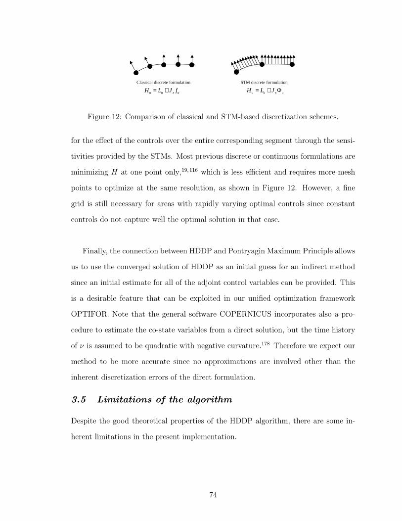
Classical discrete formulation STM discrete formulation

uxuu fJLH += uxuu JLH Φ+=

Figure 12: Comparison of classical and STM-based discretization schemes.

for the effect of the controls over the entire corresponding segment through the sensi-

tivities provided by the STMs. Most previous discrete or continuous formulations are

minimizing H at one point only,19,116 which is less efficient and requires more mesh

points to optimize at the same resolution, as shown in Figure 12. However, a fine

grid is still necessary for areas with rapidly varying optimal controls since constant

controls do not capture well the optimal solution in that case.

Finally, the connection between HDDP and Pontryagin Maximum Principle allows

us to use the converged solution of HDDP as an initial guess for an indirect method

since an initial estimate for all of the adjoint control variables can be provided. This

is a desirable feature that can be exploited in our unified optimization framework

OPTIFOR. Note that the general software COPERNICUS incorporates also a pro-

cedure to estimate the co-state variables from a direct solution, but the time history

of ν is assumed to be quadratic with negative curvature.178 Therefore we expect our

method to be more accurate since no approximations are involved other than the

inherent discretization errors of the direct formulation.

3.5 Limitations of the algorithm

Despite the good theoretical properties of the HDDP algorithm, there are some in-

herent limitations in the present implementation.

74

3.5.1 STM Computations

It has been shown that the introduction of state-transition matrices to compute re-

quired partial derivatives provides several advantages. Nevertheless, their high com-

putational cost, due to the necessity to integrate a large set of equations at each

segment, poses an important problem for the efficiency of our algorithm. A prob-

lem with n states generally requires n2 and n3 (n(n2 + n)/2 if the symmetry of the

second-order STM is taken into account) additional equations to be integrated for the

first- and second-order STMs respectively. In comparison, the traditional Ricatti-like

formulation (implemented in the software Mystic for instance259) requires only n and

n2 equations to be integrated. While the second order STM method requires a much

higher dimensioned system of ordinary differential equations, the governing equations

are much less coupled and complicated than the Ricatti-like formulation. Therefore,

a detailed efficiency comparison between the two approaches is suggested as future

work.

3.5.2 Tuning of the algorithm

Another open point is related to the tuning of HDDP. In fact, many aspects of the

algorithm require parameters that have to be tuned. For example, for the trust region

method, the parameters are the scaling matrix D (Eq. (3.31)) and the trust region

update parameter κ (Eq. (3.58)); in the augmented Lagrangian method, the initial

penalty parameter σ0 and the penalty update parameter kσ (Eq. (3.59)), and so on.

In the present implementation, these parameters are tuned a-priori, after a number of

experiments. Unfortunately, it is often observed that for different problems different

settings are required (not unlike most NLP solution methods). More research needs

to be done to find heuristic rules and select automatically the parameters to minimize

the custom efforts necessary to find a satisfactory result.

75

3.6 Improvement of efficiency

Below we mention possible approaches to significantly enhance the computational

efficiency of our algorithm.

3.6.1 Parallelization of STM computations

Once the trajectory is integrated, the STMs at each segment can be computed in-

dependently from each other. The STM calculations can therefore be executed in

parallel on a multicore machine or even a cluster to dramatically reduce the com-

putation time (see figure 13). This is a major advantage over classical formulations

where the derivatives are interconnected and cannot be computed independently.

Trajectory Integration

Partials mapping

21

11, −− ΦΦ NN

21 , kk ΦΦ20

10 ,ΦΦ 2

111,ΦΦ

Figure 13: Parallelization of STM computations.

3.6.2 Adaptive mesh refinement

Low-thrust optimal control is inherently discontinuous with a bang-bang structure.

Since the location of the switching points is known in advance, a fine equally-spaced

mesh is required to obtain an accurate solution if the mesh is kept fixed during the

optimization process. To use a more coarse mesh and reduce the computational cost,

one can employ an internal mesh optimization strategy that automatically increases

the resolution when the control undergoes large variations in magnitude.117 This leads

to an algorithm that is able to properly describe the optimal control discontinuities

by creating a mesh that has nodes concentrated around switching points.

76

3.6.3 Analytic State Transition Matrices

State transition matrices can be derived analytically for some problems.7 It is known

that low-thrust optimization software utilizing analytic STMs enjoy impressive speed

advantages compared to integrated counterparts.218,229 Our approach offers the possi-

bility to use these analytic STMs, which similarly enables tremendous computational

time savings. This promising topic will be included in the discussion of the dynamics

in Chapter 5.

3.7 Validation of HDDP

The previous sections outlined the theory and the mathematical equations that gov-

ern the HDDP algorithm. To check that HDDP works correctly, we propose to solve a

linear system with quadratic performance index and linear constraints. Powell proved

that methods based on Augmented Lagragian functions should exactly converge in

one iteration for this kind of problem.195 It comes from the fact that the augmented

cost function remains quadratic when linear constraints are included (they are only

multiplied by the Lagrange multiplier).

To test the complete algorithm, we consider a simple force-free, targeting multi-

phase problem with 2 phases (M = 2) and 5 stages for each stage (N1 = N2 = 5).

The transition functions Fi,j acting on each stage are given by:

xi,j+1 = Fi,j(xi,j, ui,j) =

ri,j+1

vi,j+1

=

ri,j + vi,j

vi,j + ui,j

for i = 1...2, j = 1...5 (3.65)

The states are the position and velocity, and the controls are directly related to the

acceleration. At each stage, the following quadratic cost function Li,j is considered:

Li,j = ‖ui,j‖2 for i = 1...2, j = 1...5 (3.66)

77

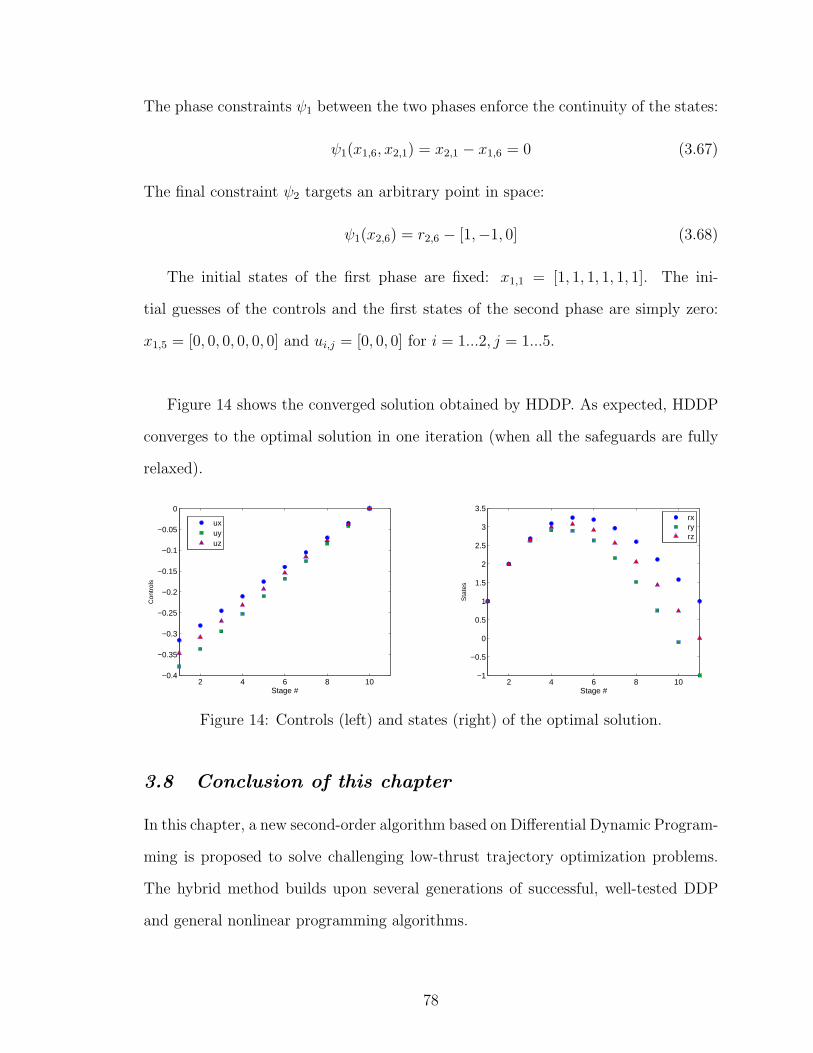
The phase constraints ψ1 between the two phases enforce the continuity of the states:

ψ1(x1,6, x2,1) = x2,1 − x1,6 = 0 (3.67)

The final constraint ψ2 targets an arbitrary point in space:

ψ1(x2,6) = r2,6 − [1,−1, 0] (3.68)

The initial states of the first phase are fixed: x1,1 = [1, 1, 1, 1, 1, 1]. The ini-

tial guesses of the controls and the first states of the second phase are simply zero:

x1,5 = [0, 0, 0, 0, 0, 0] and ui,j = [0, 0, 0] for i = 1...2, j = 1...5.

Figure 14 shows the converged solution obtained by HDDP. As expected, HDDP

converges to the optimal solution in one iteration (when all the safeguards are fully

relaxed).

2 4 6 8 10−0.4

−0.35

−0.3

−0.25

−0.2

−0.15

−0.1

−0.05

0

Stage #

Con

trol

s

uxuyuz

2 4 6 8 10−1

−0.5

0

0.5

1

1.5

2

2.5

3

3.5

Stage #

Sta

tes

rxryrz

Figure 14: Controls (left) and states (right) of the optimal solution.

3.8 Conclusion of this chapter

In this chapter, a new second-order algorithm based on Differential Dynamic Program-

ming is proposed to solve challenging low-thrust trajectory optimization problems.

The hybrid method builds upon several generations of successful, well-tested DDP

and general nonlinear programming algorithms.

78

The present algorithm makes full use of the structure of the resulting discrete time

optimal control problem by mapping the required derivatives recursively through the

first-order and second-order state transition matrices, which is in the main spirit of

dynamic programming. Convergence properties are improved, and preliminary results

demonstrate quadratic convergence even far from the optimal solution. Constraints

are included by using two different procedures: an active set constrained quadratic

programming method for hard constraints (preferably linear), and an Augmented La-

grangian method for soft constraints. For the later case, our STM-based approach is

effective because no additional integrations are needed. The possible disadvantage of

the additional cost in CPU time per iteration to compute the STMs can be also out-

weighed by several benefits, such as the exploitation of the inherent parallel structure

of our algorithm and the improved constraint handling. Further, the main compu-

tational effort involving integrations of the trajectory and sensitivities is decoupled

from the main logic of the algorithm making it modular and simpler to generalize

and experiment. The algorithm is validated on a simple dynamical problem. HDDP

will be tested on more difficult problems in Chapter 7.

One possible show-stopper in using HDDP is the need to provide exact first-and

second-order derivatives for all the functions involved in the problem (except for the

stage constraints that are only linearized). This requirement might be cumbersome

for complicated functions. To address this issue, the next chapter presents a new

method to compute automatically high-order derivatives via multicomplex numbers.

79

CHAPTER IV

MULTICOMPLEX METHOD FOR AUTOMATIC

COMPUTATION OF HIGH-ORDER DERIVATIVES

The computations of the high-order partial derivatives in a given problem are in

general tedious or not accurate. To combat such shortcomings, a new method for

calculating exact high-order sensitivities using multi-complex numbers is presented.

Inspired by the recent complex step method that is only valid for first order sensitiv-

ities, the new multi-complex approach is valid to arbitrary order. The mathematical

theory behind this approach is revealed, and an efficient procedure for the automatic

implementation of the method is described. Several applications are presented to

validate and demonstrate the accuracy and efficiency of the algorithm. The results

are compared to conventional approaches such as finite differencing, the complex step

method, and two separate automatic differentiation tools. Our multi-complex method

is shown to have many advantages, and it is therefore expected to be useful for any

algorithm exploiting high-order derivatives, such as many non-linear programming

solvers.

4.1 Introduction

Sensitivity analysis, i.e. computing the partial derivatives of a function with respect

to its input variables, is often required in a variety of engineering problems. For

instance, most optimization algorithms require accurate gradient and Hessian infor-

mation to find a solution efficiently.79 In practice, accuracy, computational cost, and

ease of implementation are the most important criteria when sensitivities must be

evaluated.

80

There are many methods for generating the desired sensitivities. First, the partial

derivatives can be analytically derived by hand, which is typically most accurate and

efficient. However, for complicated problems, this can be a tedious, error-prone and

time-consuming process. Numerical methods are therefore preferred in general. One

classical numerical method is finite differencing that finds approximation formulas of

derivatives by truncating a Taylor series of the function about a given point.35 This

technique is very simple to implement, but suffers from large roundoff errors, espe-

cially for high-order derivatives.82

Another numerical method is Automatic Differentiation (AD). Invented in the

1960s, AD is a chain rule-based evaluation technique for obtaining automatically the

partial derivatives of a function.101 AD exploits the fact that any function, no matter

how complicated, can be expressed in terms of composition and arithmetic opera-

tions of functions with known derivatives. By applying the chain rule repeatedly

to these elementary operations and functions, derivatives can be computed therefore

automatically. Some AD tools are implemented by preprocessing the program that

computes the function value. The original source code is then extended to add the new

instructions that compute these derivatives. ADIFOR32 and TAPENADE181 repre-

sents successful implementations of this approach. Other AD tools, such as AD02,199

ADOL-F227 and OCEA,247 keep the original program but use derived datatypes and

operator overloading to compute the function value and its differential at runtime.

The major advantage of all these tools is that exact derivatives can be found auto-

matically, however they generally have the drawback of being hard to implement and

computationally intensive in terms of machine time and memory. They are also often

limited to second- and in some cases first-order derivatives only.

81

Complex arithmetic can be another way to obtain accurate sensitivities. The use

of complex numbers for the numerical approximation of derivatives was introduced

by Lyness and Moler.150,151 Relying on Cauchy’s integral theorem, they developed a

reliable method for calculating the nth derivative of an analytic function from a trape-

zoidal approximation of its contour integral. Later Fornberg developed an alternative

algorithm based on the Fast Fourier Transform.82 However, both approaches are of

little practical use because they require an excessive number of function evaluations to

obtain a high accuracy. More recently, Squire and Trapp developed an elegant, simple

expression based on a complex-step differentiation to compute first-order derivatives

of an analytic function.235 They pointed out that their method is accurate to machine

precision with a relatively easy implementation. Therefore, this method is very at-

tractive and since the 2000s it has been applied in an increasing number of studies in

many fields.44,66,121,155,253 A thorough investigation on the practical implementation

of this method in different programming languages was also performed,154,155 which

makes now this technique very well understood. Note that contrary to what many

authors imply, this method is not related to the other complex approach of Lyness

and Moler, since the complex-step differentiation does not rely on the Cauchy integral

theorem. In particular, one major difference is that the complex-step differentiation

gives an expression for the first-order derivatives only, which limits greatly its range of

applications. Several extension formulas to second-order derivatives have been pub-

lished in the literature,4,133 but they all suffer from roundoff errors.

In this chapter, we describe a new way of computing second- and higher-order

derivatives by using multicomplex numbers, a multi-dimensional generalization of

complex numbers. By introducing a small perturbation into the appropriate mul-

ticomplex direction, higher-order sensitivities exact to machine precision can be re-

trieved directly from the results. As in the complex method, when the program can

82

handle multicomplex algebraic operations, no special coding is required in the func-

tion calls as the higher-dimensional space carries the underlying problem sensitivities.

Our multicomplex step differentiation (MCX) method therefore combines the accu-

racy of the analytical method with the simplicity of finite differencing.

Since standard multicomplex algebra is not built into existing mathematical li-

braries of common programming languages, an object-oriented multicomplex toolbox

(coded both in Matlab and Fortran 90) is presented to encapsulate the new data types

and extend operators and basic mathematic functions to multicomplex variables. By

exploiting some properties of multicomplex numbers, an elegant recursive operator-

overloading technique is derived to implement the overloading without much effort.

To our knowledge this is the first time multicomplex arithmetic is exploited to

generate partial derivatives of any order. We can only mention the method of Turner

who used quaternions (another extension of complex numbers) to compute all first

derivative elements of functions of three variables with a single call.246 However this

method does not evaluate high-order derivatives.

This chapter is organized as follows. First, we present the mathematical theory

behind the multicomplex step differentiation. A review of the basic definition of mul-

ticomplex numbers is given, as well as the extension of the concepts of differentiability

and holomorphism to multicomplex higher-dimensional space. Next, we investigate

how to implement in practice our method in the common programming languages

Fortran and Matlab. Finally, several applications and comparisons are presented to

validate and demonstrate the performance of the multicomplex approach.

83

4.2 Theory

In this section, the mathematical formalism associated to the multicomplex algebra

is introduced. Definitions and basic properties of multi-complex numbers are briefly

recalled. The natural multicomplex extension of differentiability and holomorphism is

given. Then the multicomplex step differentiation is proved and explained in details

with a simple numerical example.

4.2.1 Definition of Multicomplex numbers

There exist several ways to generalize complex numbers to higher dimensions. The

most well-known extension is given by the quaternions invented by Hamilton,104 which

are mainly used to represent rotations in three-dimensional space. However, quater-

nions are not commutative in multiplication, and we will see later that this property

prevents them from being a suitable for computing partial derivatives.

Another extension was found at the end of the 19th century by Corrado Segre who

described special multi-dimensional algebras and he named their elements ‘n-complex

numbers’.225 This type of number is now commonly named a multicomplex number.

They were studied in details by Price198 and Fleury.81

To understand a multicomplex number, we can recall first the definition of the

set of complex numbers, C, which should be more familiar to the reader. C can be

viewed as an algebra generated by the field of real numbers, R, and by a new, non-real

element I whose main property is i2 = −1.

C := {x+ yi / x, y ∈ R} (4.1)

The same recursive definition applies to the set of multicomplex numbers of order

n and defined as:

84

Cn :={z1 + z2in / z1, z2 ∈ Cn−1

}(4.2)

where i2n = −1, C1 := C, C0 := R.

This formula emphasizes the formal similarity of complex and multicomplex num-

bers. We will take advantage of this observation in the next section.

Other useful representations of multi-complex numbers can be found by repeti-

tively applying Eq. (4.2) to the multi-complex coefficients of lower dimension. De-

composing z1 and z2 from Eq. (4.2), we obtain:

Cn :={z11 + z12in−1 + z21in + z22inin−1 / z11, z12, z21, z22 ∈ Cn−2

}(4.3)

In the end, it is clear (see Eq. (4.4)) that we can represent each element of Cn

with 2n coefficients in R: one coefficient x0 for the real part, n coefficients x1, ..., xn

for the ‘pure’ imaginary directions, and additional coefficients corresponding to ‘cross

coupled’ imaginary directions. We note that the cross directions do not exist in R or

C, but appear only in Cn for n ≥ 2. For instance, to make the notation of Eq. (4.4)

more clear, one can make the analogy between i1i2 and the standard product of the

imaginary directions i1 and i2, which implies that (i1i2)2 = (i1)2(i2)2 = (−1)(−1) = 1

and i1i2 = i2i1.

Cn := {x0 + x1i1 + ...+ xnin + x12i1i2 + ...+ xn−1nin−1in + ...+ x1...ni1...in

/ x0, ..., xn, ..., x1...n ∈ R} (4.4)

In addition, another way to represent multicomplex numbers is with matrices. In

fact, it has been shown that every linear algebra can be represented by a matrix alge-

bra.31 One common example is the 2×2 matrix representation of complex numbers.63

85

The following theorem extends this result to Cn.

Theorem 1

Let matrix I0 be the identity matrix. In addition, let matrices I1, ..., In be the matrix

representations of the multicomplex imaginary basis elements i1, ..., in with the prop-

erty I2k = −I0 for all k ≤ n. These matrices can be constructed by recursion in the

same way as the proof of this theorem in Appendix B.1, after reordering the indices

properly to be consistent with the representation of Eq. (4.4).

Then the set of 2n × 2n real matrices of the form

M = x0I0 + x1I1 + ...+ xnIn + x12I1I2 + ...+ xn−1nIn−1In + ...+ x1...nI1...In (4.5)

is isomorphic to the multicomplex algebra Cn. Thoses matrices are called Cauchy-

Riemann matrices in the literature.198 In other words, there’s a one-to-one correspon-

dence between Cauchy-Riemann matrices of this form and multicomplex numbers.

Arithmetic operations (+,−, x) on multicomplex numbers become then equivalent to

arithmetic operations on their matrix representations. The proof of this theorem is

given in Appendix B.1.

In summary, we just reviewed three different representations of multicomplex num-

bers. We point out that the representations are not simply a matter of notational

consequence. To the contrary, they will be essential to the development of the theory.

To illustrate the various definitions, we consider several particular examples. First,

we define the elements of C2, called bicomplex numbers. Among all the multicomplex

numbers, they are the most known and studied, and have been used in several appli-

cations like fractals and quantum theory.207,208 As shown in Eq. (4.6), a bicomplex

number is composed of two complex numbers or four real numbers. It can also be

represented by a 2× 2 complex matrix or a 4× 4 real matrix.

86

C2 := {z1 + z2i2 / z1, z2 ∈ C}

:= {x0 + x1i1 + x2i2 + x12i1i2 / x0, x1, x2, x12 ∈ R}

↔

z1 −z2

z2 z1

/ z1, z2 ∈ C

↔

x0 −x1 −x2 x12

x1 x0 −x12 −x2

x2 −x12 x0 −x1

x12 x2 x1 x0

/ x0, x1, x2, x12 ∈ R

(4.6)

Another example is an element of C3, called a tricomplex number. As the dimen-

sions of the corresponding matrices become unreasonably large, they are not given

here. As shown in Eq. (4.7), a tricomplex number is composed of two bicomplex

numbers, four complex numbers, or eight real numbers.

C3 :={z1 + z2i3 / z1, z2 ∈ C2

}:= {z11 + z12i2 + z21i3 + z22i2i3 / z11, z12, z21, z22 ∈ C}

:= {x0 + x1i1 + x2i2 + x3i3 + x12i1i2 + x13i1i3 + x23i2i3 + x123i1i2i3

/ x0, x1, x2, x3, x12, x13, x23, x123 ∈ R} (4.7)

Finally, one last property of importance is that multicomplex addition and mul-

tiplication are associative and commutative, contrary to quaternions. In fact, from

Eq. (4.4), the product of two elements of Cn is obtained by multiplying those two

elements as if they were polynomials and then using the relations i2k = −1. However,

contrary to the complex numbers, the multicomplex numbers do not form a ring since

they contain divisors of zero (the product of two non-zero multicomplex numbers can

be equal to zero). This can be an issue for numerical computations as unexpected

zeroed results may be generated when two divisors of zero happen to be multiplied

87

together. In his book,198 Price shows that those divisors have a very specific form (see

Appendix B.2), and are therefore extremely unlikely to be encountered in practice.

4.2.2 Holomorphic Functions

We recall now the notion of differentiability and holomorphicity in multicomplex

analysis. This is a natural next step, since the power of multicomplex numbers in

computing derivatives cannot be exploited until a full theory of multi-complex holo-

morphic functions is developed. For this discussion we will rely essentially on the

work of Price.198 We give the definitions of multicomplex differentiability and holo-

morphism, and we present a theorem that will be necessary for the derivation of the

formulas of multicomplex step differentiation.

Definition 1

A function f : Cn → Cn is said to be multicomplex differentiable at z0 ∈ Cn if the

limit

limz→z0

f(z)− f(z0)

z − z0

(4.8)

exists. This limit will be called the first derivative of f at z0 and will be denoted by

f ′(z0).

Definition 2

A function f is said to be holomorphic in a open set U ⊂ Cn if f ′(z) exists for all z ∈ U .

This definition is not very restrictive, most usual functions are holomorphic in Cn.

Examples of non-holomorphic functions are the modulus and absolute value functions

at zero.

88

Theorem 2

Let f : U ⊂ Cn → Cn be a function, and let also f(z1 +z2in) = f1(z1, z2)+f2(z1, z2)in

where z1, z2 ∈ Cn−1. The following three properties are equivalent:

1. f is holomorphic in U .

2. f1 and f2 are holomorphic in z1 and z2 and satisfy the multicomplex Cauchy-

Riemann equations:

∂f1

∂z1

=∂f2

∂z2

and∂f2

∂z1

= −∂f1

∂z2

(4.9)

3. f can be represented, near every point z0 ∈ U , by a Taylor series.

This theorem can be obtained from results in Reference 198. The equivalencies

(1) = (2) and (1) = (3) were stated and proved in Theorem 24.2 and Theorem 27.1

respectively only for the special case n = 2 (bicomplex functions). Nevertheless, the

same methods used can be employed to prove the theorem in the general case.

4.2.3 Multicomplex Step Differentiation

We now proceed to the main purpose of the chapter. Relying on the third property

of theorem 2, Taylor series expansions are performed and used to analytically demon-

strate that the introduction of perturbations along multicomplex imaginary directions

allows us to recover the partial derivatives of any order of a holomorphic function.

To facilitate the addition of perturbations along imaginary directions, we use the

multicomplex representation of Eq. (4.4). For convenience, we must also define a new

imaginary function that retrieves the real coefficient of a specified imaginary part of

a multicomplex number.

89

Definition 3

Let z ∈ Cn be given by Eq. (4.4). The function Imσk{1,...,n} : Cn → R is defined to be:

Imσk(z) = xσk (4.10)

where σk = σk {1, ..., n} are all the combinations of the {1, ..., n} set of the following

form:

σk {1, ..., n} = 1...1︸︷︷︸k1 times

... n...n︸︷︷︸kn times

(4.11)

for k1 ∈ {0, 1}, ..., kn ∈ {0, 1}, and k1 + ... + kn = k ≤ n. For instance, for n = 3,

σ3 {1, 2, 3} = {123}, σ2 {1, 2, 3} = {12, 13, 23} and σ1 {1, 2, 3} = {1, 2, 3}.

To introduce our main result, for simplicity we start first with a function of one

variable only. We demonstrate how to obtain the nth-order derivative. Let f : U ⊂

Cn → Cn be a holomorphic function in U . Then from theorem 2, f can be expanded

in a Taylor series about a real point x as follows:

f(x+ hi1 + ...+ hin) = f(x) + (i1 + ...+ in)hf ′(x) + (i1 + ...+ in)2h2f′′(x)

2+ ...

+(i1 + ...+ in)nhnf (n)(x)

n!+ (i1 + ...+ in)n+1hn+1f

(n+1)(x)

(n+ 1)!+O(hn+2) (4.12)

From the multinomial theorem,

(i1 + ...+ in)k =∑

k1,...,knk1+...+kn=k

n!

k1!...kn!ik11 ...i

knn (4.13)

We focus on the single term on the right hand side of Eq. (4.13) containing the

product i1...in of each of the imaginary directions (corresponding to the last imag-

inary component in Eq. (4.4)). Since i2k = −1 for k = 1...n, it is clear that the

only possibility to obtain such a term is to have k1 = 1, ..., kn = 1 (kp = 0 where

p = 1...n means that ip is not present, and kp = 2 will make ip disappear as well since

i2p = −1). This combination is only allowed in the (i1 + ... + in)n term. In fact, for

(i1 + ... + in)k where k < n, one of the kp’s in Eq. (4.13) must be equal to zero and

90

for (i1 + ...+ in)n+1, one of the kp’s must be greater than 1.

From Eq. (4.12), if we ignore terms O(hn+2) we can see that the (i1 + ... + in)n

term is the only one associated to the nth-order derivative f (n). Since the i1...in

product uniquely appears in (i1 + ...+ in)n, we can deduce that the real coefficient of

the i1...in imaginary direction is a function of the nth-order derivative f (n) only (i.e.

no other derivatives involved). We can take advantage of this result by applying to

both sides of Eq. (4.12) the imaginary function corresponding to the i1...in product

(see Eq. (4.10)). Noting that n!1!...1!

= n! and dividing both sides by hn, we get an

expression of f (n)(x) with approximation error O(h2):

f (n)(x) =Im1...n(f(x+ hi1 + ...+ hin))

hn+O(h2) (4.14)

For a small step size h, this expression can be approximated by:

f (n)(x) ≈ Im1...n(f(x+ hi1 + ...+ hin))

hn(4.15)

It is easy to extend this result to obtain the nth-order partial derivatives of any

holomorphic function of p variables:

∂fn(x1, ..., xp)

∂xk11 ...xkpp

≈Im1...n(f(x1 + h

∑j∈Π1

ij, ..., xp + h∑

j∈Πpij))

hn

where

p∑j=1

kj = n,Πj = ∅ if kj = 0,Πj =

{j−1∑l=1

kl + 1, ...,

j∑l=1

kl

}if kj > 0 (4.16)

which we will call the multicomplex step derivative approximation. Notice that this

estimate is not subject to subtractive cancellation error, since it does not involve any

difference operation, contrary to finite differencing. From the same single function

call, it is also possible to retrieve the corresponding low-order partial derivatives.

∂fk(x1, ..., xp)

∂xk′11 ...x

k′pp

≈Imσk′1

{Π1}...σk′p{Πp}(f(x1 + h

∑j∈Π1

ij, ..., xp + h∑

j∈Πpij))

hk

where

p∑j=1

k′j = k < n, k′j ≤ kj (4.17)

91

For example, the particular formulas to compute the full Hessian of a function of

two variables are the following:

∂f 2(x, y)

∂x2≈ Im12(f(x+ hi1 + hi2, y))

h2(4.18a)

∂f 2(x, y)

∂y2≈ Im12(f(x, y + hi1 + hi2))

h2(4.18b)

∂f 2(x, y)

∂xy≈ Im12(f(x+ hi1, y + hi2))

h2(4.18c)

∂f(x, y)

∂x≈ Im1(f(x+ hi1 + hi2, y))

h=Im2(f(x+ hi1 + hi2, y))

h(4.18d)

∂f(x, y)

∂y≈ Im1(f(x, y + hi1 + hi2))

h=Im2(f(x, y + hi1 + hi2))

h(4.18e)

Finally note that these results are not possible using quaternions or any non-

commutative extension of complex numbers. In such cases, the multinomial theorem

of Eq. (4.13) fails and the i1...in imaginary coefficient vanishes. For instance, since

the imaginary units i, j, k of quaternions are anti-commutative under multiplication

(ij = −ji = k), we have (i+ j)2 = −2, which is a real number only.

4.2.4 Simple Numerical Example

To illustrate Eq. (4.16) and Eq. (4.17), we consider the following standard holomorphic

test function that many authors have previously used:4,133,151,155,235

f(x) =ex√

sinx3 + cosx3(4.19)

The exact first-, second-, and third-order derivatives at x = 0.5 are computed ana-

lytically and compared to the results given by the multicomplex step, the hybrid finite

difference complex-step scheme developed by Lai,133 and the central finite-difference

formulas for step sizes in the range 10−100 ≤ h ≤ 1. Since Lai does not give a formula

for third-order derivatives, we derived our own approximated expression by applying

Taylor series expansions on several complex perturbation steps:

f (3)(x) ≈ Im (f(x+ ih)− f(x+ 2ih)− f(x− ih))

h3(4.20)

92

10−100

10−80

10−60

10−40

10−20

100

10−20

10−15

10−10

10−5

100

105

Step Size (h)

Nor

mal

ized

Err

or

MultiComplex−StepComplex−step+FDFinite Difference

10−100

10−80

10−60

10−40

10−20

100

10−20

10−15

10−10

10−5

100

105

Step Size (h)

Nor

mal

ized

Err

or


10−100

10−80

10−60

10−40

10−20

100

10−20

10−15

10−10

10−5

100

105

Step Size (h)

Nor

mal

ized

Err

or


Figure 15: Normalized error: first-order derivative (left), second-order derivative (cen-ter), third-order derivative (right). Analytical estimate is the reference.

The multicomplex step method is exact to machine precision for both first and

second-order derivatives with step sizes below 10−8. In addition, since the MCX ap-

proach is not subjected to subtraction cancellations, we can choose extremely small

step sizes with no loss of accuracy. As expected, for first-order derivatives our method

gives identical results as the complex-step method while outperforming the central

difference scheme. However, for higher-order derivatives, the complex-step method

and central differences both suffer from subtraction errors. Note that in those cases

the accuracy improvement of the complex-step method over finite differences is negli-

gible. It was even observed that the formula given by Lai is not numerically stable as

its associated error goes to infinity (not shown on the plots to preserve similar scales).

Finally, we observe that finite precision arithmetic imposes a practical lower limit

on the step size h, and consequently an upper limit on the order of the derivative

calculation. In fact, when double precision numbers are used, the smallest non-zero

number that can be represented is 10−308, and hn must be therefore greater than this

number to prevent underflow in Eq. (4.16): hn > 10−308. Also, h must be small since

the error of the approximation in Eq. (4.16) is on the order of h2 (see Eq. (4.14)). To

maintain approximate machine precision, h2 < ε ≈ 10−16. It follows then for double

93

precision arithmetic:

n <log(10−308)

log(10−8)≈ 38 (4.21)

In order to further prevent the underflow situation, it is also necessary to keep some

margin to take into account the inherent dynamical magnitude excursion of internal

variables during function evaluation. Therefore, it may be unreasonable to expect

high precision with n = 38. Note that a complex number with n = 35 is represented

with 235 > 1010real numbers. Even modern computers with extraordinary memory

capacity will not have enough storage to operate on multicomplex function calls in

dimensions as high as 35.

10−80

10−60

10−40

10−20

100

10−20

10−15

10−10

10−5

100

105

h step

Rel

ativ

e E

rror

s

1th derivative

2nd derivative

3rd derivative

4th derivative

5th derivative

6th derivative

Large choice for step hε machine precision

h5 & h6 underflow limitation

Figure 16: 1st to 6th-order derivative relative errors

The limitation of the step size h is illustrated in Figure 16 where computation

errors of the test function (Eq. (4.19)) up to the 6th-order derivative are calculated

for step h from 10−70 to 1.

94

4.3 Implementation

We now describe in details how to implement in practice the formulas given in the

previous section. For completeness, computer details are discussed within two differ-

ent types of programming frameworks: the compiled language Fortran for its speed,

and the interpreted language Matlab for its ease of use. Of course, nothing is pre-

venting the multicomplex adaptation to other languages like C++ or Java.

The objective is to develop a separate module or toolbox to support multicomplex

arithmetic. The two main required capabilities are: 1) define derived datatypes to

represent multicomplex variables, and 2) overload operators and intrinsic functions

for allowing usual operations.

4.3.1 Implementation of multicomplex variables

The first step is to define the multicomplex variables. From Eq. (4.2), we choose the

recursive data structure where a multicomplex variable of order n is composed of two

multicomplex variables of order n− 1.

z = {z1, z2} (4.22)

In addition to being valid for any order n, another advantage of this structure is its

convenience regarding extensions of operators and functions as we shall see in the

next subsection.

In Matlab, this structure can be directly declared as recursive using a class state-

ment, so only one definition is needed to include multicomplex numbers of any order.

In the structure an additional integer field permits the retrieval of the order of the

multicomplex variable. On the other hand, Fortran cannot handle recursive struc-

tures, so one definition per order is necessary. For instance, for multicomplex numbers

95

of order 2 and 3, the syntax in Fortran is the following:

1: {Bicomplex number definition}

2: type bicomplex

3: double complex :: z1

4: double complex :: z2

5: end type

6: {Tricomplex number definition}

7: type tricomplex

8: type(bicomplex) :: z1

9: type(bicomplex) :: z2

10: end type

z

z1 z2

z11 z12 z21 z22

x0 x1 x1…n-1 xn x1…n

Re(z) Im1(z) Im1...n-1(z) Imn(z) Im1...n(z)

in

in-1in-1

Figure 17: Tree Representation of a multicomplex number of order n.

Additionally, in order to implement Eq. (4.16) and apply imaginary perturbation

steps, it is also necessary to decompose a multicomplex variable into strictly real

coefficients of its individual imaginary components. Furthermore, the left side of

Eq. (4.16) requires the implementation of the Imaginary function Im() that extracts

desired individual imaginary elements. To satisfy those two requirements, we require

a mapping from the current recursive representation of Eq. (4.2) to that of the real

coefficient representation of Eq. (4.4). This conversion can be deduced from the simple

tree of Figure 17 that decomposes successively one multicomplex number into into

two multicomplex numbers of lower order. Moving all the way down the tree allows us

96

to locate one specific imaginary element from a multicomplex number, which serves

as a basis of implementation for the Im function. In the same way, by traversing up

the tree, we define a multicomplex variable according to all its imaginary components

and associated real coefficients.

4.3.2 Operator and Function Overloading

It is necessary to redefine operational rules so that they can take multicomplex num-

bers as arguments. This procedure is called overloading. This should involve basic

math operations (+,−,×,/, ), relational logic operators (<,>,==), standard library

functions (sin, asin, exp, ln, ...), and linear algebra operations (matrix-vector oper-

ations, matrix inversion, eigenvalue computations‘).

4.3.2.1 Basic functions and operations

The recursive multicomplex representation we selected in the previous subsection

makes the extension of any operation and function definition quite simple. In fact,

with this representation, it turns out that arithmetic operations on multicomplex

numbers are completely identical to respective operations on complex ones. For ex-

ample, the multiplication of two multicomplex numbers has the following form:

z × w = (z1 + z2in)(w1 + w2in) = (z1w1 − z2w2) + (z1w2 + z2w1)in (4.23)

which is the exact same form as the complex multiplication. The same property can

be observed for any other function or operation. This result can be readily deduced

from Eq. (4.2) where it is clear that multicomplex numbers have the same general form

as complex numbers. Since i2n = −1 in Eq. (4.2), operation rules will be the same for

complex and multicomplex numbers. It follows that we can re-use the same existing

complex number overloading routines for complex numbers. The only change required

is to replace the complex datatype with the corresponding multicomplex datatype.

This results in a very elegant and simple implementation.

97

4.3.2.2 Relational logic operators

Regarding relational logic operators, we decided to follow the same strategy as Mar-

tins.155 These operators are usually used inside conditional statements which may

lead to different execution branches. To compute correct derivatives, the execution

branch should stay the same whether the calculations are in made with real or mul-

ticomplex numbers. It follows that only the real parts of the arguments should be

compared.

4.3.2.3 Linear algebra

Enabling linear algebra capabilities demands extra care. Here, at least two strategies

are possible. First, linear algebra algorithms can be re-written to support multicom-

plex arguments. However, this can be a tedious process. For instance, in Fortran, lin-

ear algebra routines are commonly provided by the LAPACK package which consists

of hundreds of cryptic separate routines (for Gaussian elimination, LU factorization,

QR factorization ...). In Matlab the situation is even worse as linear algebra routines

are built-in and cannot be accessed.

A second strategy is to take advantage of the matrix representation of Eq. (4.5).

By mapping multicomplex variables to higher-dimensional real- or complex-valued

matrices, we can use directly existing real or complex built-in algorithms, at the

expense of memory usage. For instance, to solve the multicomplex linear matrix

equation Az = b where A ∈ Cn p×p, z ∈ Cn p×1, b ∈ Cn p×1, we can carry out the

following transformation of A:

A↔M = A0I0+A1I1+...+AnIn+A12I1I2+...+An−1nIn−1In+...+A1...nI1...In (4.24)

where A0, ..., A1...n ∈ Rp×p and the expressions for the I ′ks are given in theorem 1 (note

that in the formula the 1′s represent real identity matrices of dimension p× p). The

98

matrix equation becomes:

M︸︷︷︸2np×2np

x0

...

x1...n

︸︷︷︸

2np×1

=

b0

...

b1...n

︸︷︷︸

2np×1

(4.25)

where x0, ..., x1...n ∈ Rp×1 and b0, ..., b1...n ∈ Rp×1.

Eq. (4.25) is solved as a real-valued matrix equation for x0, ..., x1...n. We can follow

the exact same approach for other linear algebra algorithms like matrix inversion and

eigenvalue problems. A similar strategy is used by Turner in his quaternion toolbox.248

4.3.3 Overall Procedure

The multicomplex step differentiation procedure can be summarized as follows:

1. Convert the function code to support multicomplex arithmetic. In Matlab, no

change in the code is necessary and the user just needs to include the multi-

complex toolbox in the path. However, in a Fortran code, all real types of the

independent variables should be substituted with multicomplex declarations.

In addition, if the value of any intermediate variable depends on the indepen-

dent variables via assignment or via argument association, then the type of

those variables must be changed to multicomplex as well (an easier yet memory

inefficient option is to declare all variables multicomplex). The user enables

overloading by simply inserting a ‘use module’ command for the module that

contains all the multicomplex extensions and definitions. All these manipula-

tions imply obviously that the user must have access to the source code that

computes the value of the function. To avoid having several versions of the

same code supporting different types of variables, one can use a preprocessor

99

that automatically produces a single code that can be chosen to be real or

multicomplex at compilation.

2. Apply small perturbation steps to the imaginary directions of the desired inde-

pendent variables and compute the resulting function value.

3. Retrieve the corresponding partial derivatives using Eq. (4.16) and Eq. (4.17).

4. Repeat steps 3-4 for all variables and all partial derivatives.

For a real-valued function of p variables, this technique requires pn function eval-

uations to compute all the partial derivatives up to nth order, compared to (np+ 1)n

and (2np + 1)n function evaluations respectively for forward and central differences.

If symmetries are considered, the number of function evaluations can be reduced by

almost half (this is also true for finite differencing). More generally, if the sparsity

pattern of the partial derivatives is known, our approach allows us to compute only

the relevant non-zero components to save compute time.

In summary, our method shares with automatic differentiation the capability of

computing systematically accurate partial derivatives with respect to desired input

variables. However, a major difference is that the user has control on which compo-

nents they want to compute by applying a perturbation step on specific imaginary

directions and computing a series of multicomplex function evaluations. From that

point of view, our approach is close to finite differences. Therefore, the multicomplex

method could be classified as semiautomatic differentiation.

4.4 Applications

Three examples of derivative-based applications illustrate the multicomplex step tech-

nique. The first one is a formal benchmark example. The next two are practical

applications from the astrodynamics area. In all cases we compare the accuracy and

100

computational cost between our approach and current other approaches, namely ana-

lytical differentiation, automatic differentiation and finite differences. In this section

all the computations are performed on a PC in Fortran 90 with an optimization level

of 2. Two different automatic differentiation tools are selected for the numerical

comparisons:

• the new package AD02 from the HSL library. This tool relies on operator

overloading to carry along derivative computations to the arithmetic operators

and intrinsic functions.199 It is one of the only automatic differentiation tools

that allows the computation of high-order derivatives (i.e. order greater than

two).

• the TAPENADE software, developed at INRIA (Institut National de Recherche

en Informatique et Automatique). Contrary to AD02, it is a source transforma-

tion tool. Given a source program, this tool returns the first-order differentiated

program.181 By applying TAPENADE several times, the code for higher-order

derivatives can be obtained as well. Note that this method for computing higher-

order derivatives is somewhat tedious and not optimal from a complexity point

of view.

We caution readers not to necessarily take the following results as an indication of

the performance that could be expected on their code. Specificities of the problems

play an important factor and some tools might perform better or worse depending on

the applications.

4.4.1 Simple Mathematical Function

First, to check the correct implementation of the multicomplex method, the same sim-

ple one-dimensional function of section 4.2.4 (Eq. (4.19)) is used for the comparisons.

Sensitivities up to third order are computed. From the right plot of Figure 15, the

multicomplex and finite difference derivatives are computed using a step size of 10−40

101

and 10−4 respectively. The analytical expressions of the derivatives are found with

the help of the algebraic manipulation software, Maple, and optimized by introduc-

ing temporary intermediate variables to eliminate redundant computations. Table 2

summarizes the results of the comparison.

Table 2: Simple function example.

Method 3rd-order Max. relative Relativederivative difference computational time

Analytical -9.33191003819869 0.0 1.0MultiComplex Step -9.33191003819869 1.9 10−16 37

AD02 -9.33191003819869 3.8 10−16 149TAPENADE -9.33191003819869 3.8 10−16 8

Finite Differences -9.33197963348675 7.4 10−6 3.5

Among methods that provide exact derivatives, the analytical and TAPENADE

methods are by far the fastest. This is explained by the fact that they produce

dedicated optimized code for the derivatives. However some implementation work

to obtain the executable programs for computing the derivatives is necessary for

those two methods. While this effort is significant for the analytical approach, this

preliminary step is straightforward in the TAPENADE case as the source code needs

only to be processed by the tool without any changes. On the other hand, the

multicomplex and AD02 methods require very little change in the source code, but

are slower for this simple test case. We point out that the multicomplex method is less

computational intensive than AD02, which shows the advantage of our method among

overloading techniques. Finally, we can say that finite difference is fast, but exhibits

very poor accuracy. In this particular example, the small difference in computational

speed between the analytical and finite difference cases is explained by the fact that

the analytical expressions of the derivatives are quite complicated in comparison to

the function (Eq. (4.19)) alone.

102

4.4.2 Gravity Field Derivatives

For this example, the first-, second- and third-order partial derivatives of the grav-

itational potential of a non-spherical body with respect to cartesian coordinates are

considered. These sensitivities are important for solving a variety of problems in

satellite geodesy and navigation. For instance, the gravitational acceleration at any

given location is obtained by computing the gradient of the potential. This acceler-

ation is required for accurate numerical integration of satellite orbits. Additionally,

the second- and third-order derivatives can be used in a variety of targeting or opti-

mization problems that arise in spacecraft guidance and navigation.

The analytical method we employ is based on the classical spherical harmonic

formulation where the derivatives are formed by exploiting recurrence relations on

Legendre polynomials.244 Finite differencing is not considered for this example as we

saw in Figure 15 that its accuracy is extremely poor for high-order derivatives.

We use a 20 × 20 lunar gravity field model taken from GLGM-2 data,142 which

corresponds to 440 terms. The position vector in cartesian coordinates where the

derivatives are estimated is (x, y, z) = (2000, 0, 0) km, which corresponds to an alti-

tude of about 300 km from the surface of the Moon. A step value of h = 10−40 is

taken in our multicomplex method. We use tricomplex numbers since derivatives are

computed up to the third-order.

The resulting accuracy and computational comparison is made in Table 3. A

sample of the third-order derivatives (corresponding to the (1,1,1) index) produced

by each method is given, as well as relative computational time and maximum rel-

ative difference of all partial derivatives with respect to the analytical expressions.

We know that the potential is a solution to Laplace’s equation. Then, in cartesian

103

coordinates, ∇2U = Uxx + Uyy + Uzz = 0. A good indicator of the accuracy of each

method is therefore the deviation from zero of the corresponding Laplacian.

Table 3: Lunar gravitational potential example.

Max RelativeMethod Sample 3rd-order Sensitivity Laplacian difference comp.

timeAnalytical −4.239541972305253 10−12 −8.3 10−25 0.0 1.0

MultiComplex Step −4.239541972305250 10−12 −4.1 10−25 6.0 10−15 20.9AD02 −4.239541972305255 10−12 −1.1 10−24 2.9 10−15 154.9

TAPENADE −4.239541972305257 10−12 −1.6 10−24 2.6 10−15 30.1

As expected, the analytical method is by far the fastest. Its implementation

relies on a very efficient use of recurrence relations to reduce as much as possible the

amount of computations. Therefore this method is very specific and not representative

of the general situation (see next example for instance). It is included here only

to provide a benchmark as any other method is likely to be far slower. Taking

that into account, we can see that multicomplex step method is also accurate to

machine precision while being reasonably fast (only one order of magnitude slower). In

comparison, AD02 produced very accurate estimates, but it was more computational

intensive, more than seven times slower than the multicomplex method. In this

example it is apparent that the computational overhead of AD02 is again significantly

larger than that of the multi-complex method. Finally, contrary to the previous

simple example, TAPENADE is also slower than the multicomplex method. This

may come from the multidimensional aspect of the problem as TAPENADE does

not take advantage of the symmetries and computation redundancies of higher-order

derivatives (TAPENADE is designed to produce first-order derivative code only.).

104

4.4.3 Trajectory State Transition Matrix

Another application is presented for a low-thrust spacecraft trajectory problem where

the multicomplex approach is used to generate first- and second-order state transi-

tion matrices.15 The trajectory model consists of an orbiting satellite subject to the

Sun gravitational force and a constant inertial thrust. This kind of dynamical model

often occurs in direct optimization methods when a low-thrust trajectory is divided

into several segments of constant thrust.255 To optimize the resulting set of thrust

variables, partial derivatives of the final state vector with respect to the initial state

vector of a given segment are usually required to help the solver converge toward an

optimum. These sensitivities are the components of the so-called State Transition

Matrices which map derivatives from one time to another on a given continuous tra-

jectory.152 Because such optimization problems are highly non-linear in nature, it is

recommended to compute accurate first-and second-order derivatives to enable robust

convergence.25 The objective of this example is therefore to compute the first- and

second-order state transition matrices of one low-thrust trajectory segment.

Table 4: Data of the trajectory propagation

Parameter ValueGravitational Parameter 1.3267 1020m3s−2

Initial radius 1.496 1011 mInitial velocity 2.9783 104 m/s

Initial mass 680 kgThrust Magnitude 0.56493 NThrust Direction 0o

Isp 5643 sTime of Flight 6 days

Numerical data used for the propagation are given in Table 4 and are mainly taken

105

from Oberle.176 The motion is two-dimensional and restricted to be in the heliocen-

tric plane. The satellite starts in a circular orbit with the position and velocity of the

Earth. The variables to be integrated are then the position and velocity states (four

polar coordinate variables), the satellite mass (1 variable) and the control variables

(two variables). The trajectory propagation is therefore a seven-dimensional integra-

tion.

The standard analytical method integrates directly the state transition matri-

ces from analytical derivatives of the equations of motion.152 This results in a

very large system to integrate with 7 + 7 ∗ 7 + 7 ∗ 7 ∗ 7 = 399 dimensions. Sym-

metry and sparsity patterns can be exploited to reduce this number to at most

5+(7∗5)+5∗(7∗7+7)/2 = 180 dimensions (noting that the control is static). Because

such improvements are tedious to implement in the analytic integration of the STMs,

the numbers in Table 5 reflect the dense and straight-forward implementation with

399 terms. For the multicomplex step differentiation and finite differences, the numer-

ical STM partial derivatives are computed by integrating the original 7-dimensional

propagation problem several times for different perturbation steps. In these cases,

unlike the analytic case, the sparsity and symmetry patterns of the STMs are easily

implemented, and we emphasize that the associated benefit is reflected in the com-

pute times presented in Table 5. For all methods a standard 7th-order Runge-Kutta

integrator is used to generate the results. Relative and absolute integration tolerances

are set to 10−13 for maximum accuracy. Step sizes of h = 10−40 and h = 10−4 are

taken for the multicomplex step and finite difference methods respectively. For finite

differences, this step size is obtained after several trial-and-errors to find the best

accuracy (this trial and error effort is not included in the speed results). Standard

central finite difference formulas are used in the calculations. The reported times and

max relative differences reflect the calculation of the full first and second order STMs.

106

The sample spherical component is the term∂2rf∂2r0

.

Table 5: State transition matrix example for low-thrust spacecraft trajectory.

Method Sample 2nd-order STM Max. relative RelativeComponent difference computational time

Analytical −2.092290564266828 10−2 0.0 1.0 a

MultiComplex Step −2.092290564266829 10−2 5.3 10−15 1.7AD02 −2.092290564266833 10−2 4.0 10−14 4.4

TAPENADE −2.092290564266826 10−2 3.7 10−14 2.1Finite Differences −2.092290785071782 10−2 2.8 10−6 4.5

We can see that the analytical method is again the fastest, but by a much smaller

margin than the previous example. This is explained by the fact that a large cou-

pled system has to be integrated. The multicomplex approach is still accurate to

machine precision with only a very slight computational handicap. Considering the

effort needed to implement the analytical approach, the competitiveness of our ap-

proach becomes evident. By comparison, both AD tools, AD02 and TAPENADE,

are slower than the MCX approach. Also note that minor changes in the code were

required to use AD02 and TAPENADE as some matrix operations (like the mat-

mul function) are not supported by these tools. Finally, Finite Difference is clearly

the least attractive approach. Its accuracy is poor and it is the slowest of all methods.

In the previous two real-world applications, we find the MCX approach faster

than that of AD02 and TAPENADE. However the improvements vary from 260% to

740% for AD02, and from 20% to 30% for TAPENADE, indicating a need to further

characterize both applications and other implementation strategies and tools.

athis time can likely be reduced by half if the aforementioned symmetries are considered.

107

4.5 Conclusions of this chapter

Many applications in scientific computing require higher order derivatives. This chap-

ter describes a promising approach to compute higher order derivatives using multi-

complex numbers. The theoretical foundation and the basic formulation of this new

multicomplex step differentiation method is rigorously introduced. This method is a

natural extension to the complex step method recently introduced and now in wide

use. The main contribution here is the extension of the complex step derivative to ar-

bitrary order while maintaining the machine precision accuracy that makes both the

complex step (for first-order derivatives) and automatic differentiation so attractive.

The main results of the chapter are formula giving general partial derivatives in terms

of imaginary coefficients of multicomplex function evaluations. The main advantage

of these expressions is that they entail no subtractive cancellation error, and therefore

the truncation error can be made arbitrarily (to machine precision) small.

In addition, an efficient implementation strategy using operator and function over-

loading is outlined. The particular representation of multicomplex numbers which

shares the same formal structure as complex numbers makes this overloading partic-

ularly simple. The implementation is tested with a simple benchmark function as well

as two real-world numerical examples using complicated function calls. The resulting

derivative estimates are validated by comparing them to results obtained by other

known methods. In both cases of the complicated function calls, the multicomplex

method is found to outperform both automatic differentiation and finite differences.

In summary, the multicomplex step method provides a complete differentiation

system capable of generating exact high-order partial derivative models for arbitrarily

complex systems. This technique combines the accuracy of automatic differentiation

108

with the ease of implementation of finite differences, while being less computation-

ally intensive than either method. We also find that the multicomplex approach is

characterized by a shorter development time than that of automatic differentiation,

as the theory and code development of the multicomplex technique described in this

chapter required only a few months to implement. Considering all these advantages

the multicomplex method is therefore expected to have a broad potential use.

Future work will apply the multicomplex method to various optimization tech-

niques, such as the second-order Newton’s method, where Jacobian and Hessian in-

formation is needed. In order to further automate the implementation, the next

step is to develop a script that generates automatically the required changes in a

code to make it compatible with multicomplex numbers (variable type declarations,

‘use’ statements, etc). Finally, we intend to exploit the inherent parallelism of the

multicomplex step method to further reduce the associated computational cost.

109

CHAPTER V

LOW-THRUST TRAJECTORY MODELS

As explained in Chapter 2, our general optimization architecture OPTIFOR relies on

building block function models that define a trajectory design problem. To incorpo-

rate this architecture into an operational tool and solve low-thrust problems, the next

step is to identify, gather and implement different algorithmic functions in libraries

that can represent different parts of a trajectory. This allows the users to select the

functions that suit their needs for an easy build up of a complete mission. In this

chapter, we give an overview of the models that are implemented in the framework.

5.1 Trajectory parameterization

First, we explain how the states and controls of the spacecraft are represented. Along

the trajectory, the spacecraft state vector is defined by 7 variables: position vector,

velocity vector and mass.

x = (r,v,m) (5.1)

In Figure 4, we saw that the trajectory is divided into phases that are bracketed by

two node points. These node points have their own position, velocity, and reference

epoch time. In general they refer to celestial bodies that the spacecraft encounter.

Their ephemerides are provided via external libraries such as JPL DE405 or SPICE,

or by a set of orbital elements at the corresponding epoch. The static control variables

for each phase are then the velocity V∞ of the spacecraft relative to the starting node

point, the mass m0 of the spacecraft at the beginning of the phase, the initial and

final values t0 and tf of the time of the phase with respect to the epoch time tepoch:

w = (V∞,m0, t0, tf ) (5.2)

110

Alternatively, the entire initial conditions can be free and included in the static

vector:

w = (r0,v0,m0, t0, tf ) (5.3)

The other set of independent variables are the dynamic control variables on each

segment. As we will see later, trajectory segments can have velocity impulses or

constant finite thrust. This choice yields three control variables at each segment: the

magnitude of the impulse approximating the thrusting ∆V or the magnitude of the

thrust itself T , and the two spherical angles α and β of the thrust direction.

u = (∆V, α, β) or u = (T, α, β) (5.4)

Finally, note that whenever an indirect formulation is used we must also the time

evolution of the costate vector:

λ = (λr,λv, λm) (5.5)

Accordingly, the initial values of the co-states must be included in the static param-

eters.

5.2 Environment Models

Kepler Model Stark ModelConstant Thrust Numerical Model

Impulsive Three Body Model

Indirect Two-Body Model

Figure 18: Implemented Propagation Models.

111

In this section, we classify different environment models along a stage according to

the forces acting on the spacecraft and the level of accuracy desired by the user. An

environment model is defined by the transition function, the stage constraints and the

associated derivatives. Five different models are selected in the thesis and are depicted

in Figure 18. They are explained in details in the following subsections. Note that

this list of models is not exhaustive and other combinations could be selected as well.

5.2.1 Kepler Model

5.2.1.1 Motivations

In the Kepler model, a segment corresponds to an impulsive ∆V followed by an

analytical Kepler propagation (see Figure 18) according to a two-body model with

respect to a primary body (Sun, Earth or other planets). Since a closed-form solu-

tion is known for the state propagation and the corresponding first- and second-order

STMs,135,190 no numerical integration of the equations of motion is needed, which

results in fast computations.

The Kepler model was proposed by Sims and Flanagan230 to approximate low-

thrust trajectories as a series of impulsive ∆V ’s connected by conic arcs (see Fig-

ure 19). The software MALTO developed at JPL,229 and GALLOP, developed at

Purdue University,159 successfully apply this technique for preliminary mission de-

sign. This simplification of the problem can reduce dramatically the number of vari-

ables, and existing analytical results of the two-body problem can be advantageously

exploited. The model is akin to using a low order Euler integration scheme on the

thrust- but a highly accurate integration method on the Keplerian motion. While n-

body, oblateness, and other perturbations may be included, the model is best suited

for near Keplerian problems. Numerical comparisons show good agreement with high-

fidelity tools.193

112

∆v0∆v1

∆vN-1

tNtN-1t1t0

xNxN-1

x1

x0

Figure 19: Impulsive discretization scheme.

Note that this formulation is also suitable for high-thrust propulsion since in that

case the impulsive ∆V ’s readily represent deep space manoeuvres. If no manoeuver is

needed at the beginning of a segment, the optimizer simply drives the corresponding

∆V magnitude to zero. The optimisation of the number of impulses as well as their

respective locations is therefore automatically tackled.

In MALTO and GALLOP, the trajectory structure from the Kepler formulation

leads to a constrained nonlinear programming (NLP) problem, which is solved di-

rectly using the nonlinear solver SNOPT.93 Even with the simplified formulation of

the problem, the number of control variables grows as the square of the flight time.

Therefore, the many revolution problem can be difficult to converge even with the

sparse capabilities of SNOPT. The resulting increased dimensionality causes direct

methods to become computationally prohibitive (‘curse of dimensionality’). In ad-

dition, only first-order derivatives are used by SNOPT (second order derivatives are

approximated at best), so convergence is slower than pure second-order methods.

The goal of this subsection is therefore to combine the convergence and low dimen-

sion benefits of HDDP with the speed and simplicity of the impulsive perturbation

model. HDDP uses first- and second-order state transition matrices (STMs) to obtain

the partial derivatives required for optimization. A problem with n states generally

113

requires n2 and n3 additional equations to be integrated for the first- and second-

order STMs. If follows that the optimization process with HDDP is computationally

intensive when HDDP uses numerical integrations to obtain the required partials. To

make this algorithm more appropriate for preliminary design, we extend it by em-

ploying the analytic STMs of the two-body problem and we intend to demonstrate

the value of using Keplerian STMs in the optimization process.

5.2.1.2 Dynamics

The state xk of the spacecraft at a node point is given by its position rk and velocity

vk. Each impulse ∆vk leads to a velocity discontinuity before and after the impulse

given by v+k = v−k + ∆vk. Also, since we will see that the mass of the spacecraft

appears in some equations, it must be computed alongside the trajectory, but is not

part of the state vector (a further reduction in the problem dimension). The mass

discontinuity due to the impulse is obtained from the rocket equation:

m+k = m−k exp(− ∆vk

g0Isp) (5.6)

The mapping between the states that form the segment boundaries is defined on

each segment by a transition function Fk :

xk+1 = Fk(xk,∆vk) (5.7)

To reduce computational time, the coast arcs are computed analytically using

two-body mechanics with respect to a primary body using a standard Kepler solver

through the “f and g” procedure presented by Bate et al.14 If the position and

velocity are known at a given instant, then the position and velocity at any later time

are found in terms of a linear combination of the initial values. Therefore we can get

a closed form expression of the transition function:

114

xk+1 =

rk+1

v−k+1

=

frk + g(v−k + ∆vk)

frk + g(v−k + ∆vk)

= Fk(xk,∆vk) (5.8)

The Lagrange coefficients f , g and their time derivatives in these expressions are

functions of initial conditions and change in anomaly. Because the independent vari-

able is time, the final solution requires iteration. We use the classic Newton-Raphson

method.14

Since ∆vk is part of the transition function, v−k is defined from now on to be

the value of the velocity at node k and superscript ’-’ can be dropped. Examples of

the type and scope of the problems that can be solved using this model include all

unperturbed and perturbed Keplerian trajectories about a single celestial body for

orbit transfers, rendezvous, intercepts, arrival and capture, departure and escape. We

will see later how to account for perturbations.

5.2.1.3 Constraints

One important stage constraint with the Kepler model is the limitation of the mag-

nitude of the impulse by the total amount of ∆v that could be produced by the low-

thrust engine over the duration of the segment. This is to ensure that the impulse

discretization scheme models accurately the corresponding low-thrust propulsion sys-

tem.

∆vk ≤ ∆vmax,k =Tmax

m−k∆t (5.9)

This formula slightly underestimates the maximum velocity impulse since only the

mass at the beginning of the segment is used, while it should be linearly decreasing

over the segment. This expression therefore leads to a more conservative trajectory

design.

115

5.2.1.4 Keplerian STMs

The analytic method relies heavily on the f and g solution of the Kepler problem

found in Eq. (5.8). We emphasize that the universal formulation allows us to handle

hyperbolic trajectories without modification although the examples we consider later

are elliptical.

The analytic first-order Keplerian state transition matrix developed by Goodyear,99

Battin15 and others70,107,141,233 is well known. It is computed via universal variables

to obtain the derivatives of the Lagrangian representation coefficients of Eq. (5.8),

since: δrk+1

δvk+1

=

δfI δgI

δfI δgI

rk

vk

+

fI gI

fI gI

δrkδvk

(5.10)

Pitkin builds upon this formulation to obtain both first- and second-order STMs.190

In our algorithm we follow the same process as Pitkin. The details of the derivation

are tedious and will not be reproduced here. There are minor differences to make the

computations more efficient. The universal variable is found from the solution of the

Kepler problem. Also, we prefer to use the closed form expression of the universal

functions given by Goodyear99 instead of truncated series as proposed by Pitkin.

In addition to a dramatic reduction in the number of variables and the availability

of analytic partial derivatives, another advantage of this formulation is that sensitiv-

ities with respect to the impulses are the same as those with respect with the state

velocity components. Therefore, unlike HDDP (or traditional DDP), we do not re-

quire extra equations of motion for the control sensitivities.

Table 6 details the dramatic computational gains achieved using the analytic

116

STMs. An improvement of three orders of magnitude can be obtained for the STM

computations. Figure 20 shows that the main computational burdens for numerical

HDDP are the STM computations and the trajectory integration while the remain-

ing calculations are negligible. On the other hand, using an analytic approach allows

a relatively even distribution of the computational burden amongst the trajectory,

STM, and sweep calculations. Note that the trajectory computation is nontrivial

despite its low dimension due to the iterations required to solve Keplers problem.

Steps Analytic HDDP Numerical HDDP

STM Computations 0.38 s 186 s

Trajectory Propagation 0.32 s 23.3 s

Backward Sweep 0.16 s 0.14 s

Other 0.05 s 0.05 s

Table 6: Execution times of HDDP steps in Matlab for a representative problem using

150 nodes.

Analytical HDDP

STM computation

42%

Trajectory Computation

35%

Backward Sweep18%

Other5%

Numerical HDDP

Trajectory Computation

11%

STM Computation

89%

Figure 20: Execution time contributions.

117

5.2.1.5 Time Derivatives

This subsection presents a method to solve the problem with variable beginning and

ending time. Since our approach does not require any integrations, no normalization

of time is needed. First, to obtain derivatives with respect to time of flight, the states

are augmented with this new variable:

X =

r

v

TOF

(5.11)

The STMs are then augmented with the corresponding extra derivatives. The

STM derivatives with respect to time of flight are found by differentiating with respect

to time the position and velocity at the end of the stage.

Φ1rt = vk+1 (5.12a)

Φ1vt = −µ rk+1

‖rk+1‖3 (5.12b)

Φ2rrt = Φ1

vr (5.12c)

Φ2rvt = Φ1

vv (5.12d)

Φ2rtt = Φ1

vt (5.12e)

Φ2vrt = −µ Φ1

rr

‖rk+1‖3 + 3µrk+1

‖rk+1‖5

∂rk+1

∂rk(5.12f)

Φ2vvt = −µ Φ1

rv

‖rk+1‖3 + 3µrk+1

‖rk+1‖5

∂rk+1

∂vk(5.12g)

Φ2vtt = −µ vk+1

‖rk+1‖3 + 3µrTk+1vk+1rk+1

‖rk+1‖5 (5.12h)

5.2.1.6 Perturbations

Like thrust, effects of perturbation forces fp can be approximated by a series of im-

pulses at each node to account for the perturbing acceleration over the whole segment.

118

The transition function and the STMs are modified accordingly.

∆vP,k ≈ fP (xk, tk)∆t (5.13)

Since this method is an approximation of the actual low-thrust dynamics, it can

fail to be accurate (especially in multi-body dynamics) unless the number of im-

pulses is drastically increased, which would slow down the optimization process. To

overcome this drawback, we introduce a more accurate model.

5.2.2 Stark Model

In the Stark model, the impulses are replaced with constant thrusting over the seg-

ment (see Figure 18). The next chapter is specifically dedicated to this model. In a

similar spirit as the Kepler case, exact closed-form solutions will be derived for this

model to enable fast computations.

5.2.3 Constant Thrust Numerical Model

The two previous analytical models involve approximations of the true dynamics and

are therefore primarily useful in the preliminary design stage. For higher fidelity

optimization, it is necessary to numerically integrate the equations of motion. The

thrust is set constant along the stage. Assuming that the thrust vector is expressed

in spherical coordinates (see Eq. (5.4)), the resulting equations of motion are the

following:

d

dt

r

v

m

=

v

−µ rr3

+ Tm

u + h(r, t)

− Tg0Isp

(5.14)

where µ is the two-body gravitational parameter, and u is the thrust unit vector:

u = (cos(α) cos(β) sin(α) cos(β) sin(β)). The function h accounts for the perturbing

119

gravitational forces of other bodies (if any):

h(r, t) = −Gnb∑j=1

mj

(r− rj(t)

‖r− rj(t)‖3 +rj(t)

r3j (t)

)(5.15)

where G is the universal constant of gravitation, nb is the number of perturbing celes-

tial bodies and mj is the mass of celestial body j. The corresponding first- and second-

order STMs are numerically integrated according to Eq. (3.21a) and Eq. (3.21b). We

can also include the effects of oblateness, solar pressure radiation, drag or other per-

turbations with additional terms in the right hand side of Eq. (5.14).

5.2.4 Impulsive Restricted Three-Body Model

Contrary to the two-body model that can take into account third-body effects only

as perturbations, the restricted three-body model allows the user to take advantage

of the special features of three-body systems, like Halo orbits or invariant manifold

trajectories. In this model, a segment corresponds to an impulsive ∆V followed by an

numerical propagation of the circular, restricted three-body equations of motion with

respect to a primary body and a secondary body (see Figure 18). A complete discus-

sion of the circular, restricted three-body problem (CR3BP) is given in Ref. 127. The

numerical propagation is carried out using a Runge-Kutta Dormand-Prince integra-

tor of order 7(8). The first- and second-order STMs can be computed using the STM

equations of motion or automatically using the multicomplex method of Chapter 4.

5.2.5 Indirect Two-Body Model

All the four previous dynamical models apply to the direct formulation of the low-

thrust problems (see section 2.1.1). In this subsection, we present the dynamics of the

indirect formulation (see section 2.1.2) in the two-body problem. Future work will

implement an indirect three-body model as well to account for multi-body dynamics.

In the indirect approach, the thrust vector must follow a steering law that satisfies

120

the conditions of optimality described in section 2.1.2 along the whole stage. The well-

known primer vector theory140,215 is now used to derive the optimal steering law. If

a two-body force model is assumed (i.e. h = 0 in Eq. (5.14)), the Hamiltonian of the

system can be written:

H = λTr v + λT

v (−µ r

r3+T

mu) + λm(− T

g0Isp) (5.16)

We can deduce from Eq. (2.3a) the costate vector equations:

λr = −Hr

= −Gλv (5.17a)

λv = −Hv

= −λr (5.17b)

λm = −λvT

m2(5.17c)

where G is a symmetric matrix that represents the gradient of the Keplerian force

with respect to the position vector:

G1,1 = µ2r2

1 − r22 − r2

3

r5

G1,2 = 3µr1r2

r5

G1,3 = 3µr1r3

r5

G2,2 = µ2r2

2 − r21 − r2

3

r5

G2,3 = 3µr2r3

r5

G3,3 = µ2r2

3 − r21 − r2

2

r5(5.18)

In addition, Eq. (2.3e) requires the minimization of H with respect to the thrust

unit vector u and the thrust magnitude T . From Eq. (5.16), H is clearly minimized

when:

u = −λvλv

, T =

0 ifS < 0

Tmax ifS > 0

0 ≤ T ≤ Tmax ifS = 0

(5.19)

121

where S is usually called the switching function:

S = λv +λmm

g0Isp(5.20)

Eq. (5.19) is called the primer vector control law. It is clear that this law is not

continuous when S changes sign (i.e. when a switching occurs). Since most solvers

require differentiability of the functions, this method often fails to converge when the

switching structure must undergo changes.

To increase the robustness of the approach we use a smoothing technique in-

troduced in Ref. 22. The discontinuity of the thrust magnitude in Eq. (5.19) is

approximated by the steep, continuous, sigmoidal function:

T =Tmax

1 + exp(−S/ε)(5.21)

where ε is a small parameter. Note that the larger ε is. the easier the solution

can be converged since the sigmoidal function becomes smoother. However, this

robustness comes at the expense of accuracy since T will be increasingly far from a

bang-bang solution as ε increases. In practice, a continuation method on ε is therefore

often used.22,67 Starting at a relatively high value of ε, successive sub-problems are

solved by slowly increasing the parameter. When ε becomes very small, the switching

structure is well approximated and the original control law of Eq. (5.19) can be safely

used to find the true optimal ‘bang-bang’ solution.

5.3 Events

A sequence of inter-phase and final constraints must be defined so that they can be

executed in the simulation. The list of possible events is the following:

• Continuity: at the end of the phase, the final states of the spacecraft (position,

velocity, mass) must be continuous and match the initial states at the start of

the next phase.

122

• Interception: the spacecraft matches the position of the body at the final time

of the phase.

• Flyby: the spacecraft matches the position of the body at the final time. In

addition, the gravity effect of the body is treated as instantaneous and modeled

by a change in the direction of the V∞ (relative velocity vector). The deflection

angle of the flyby is calculated from the incoming and outgoing relative veloci-

ties. The resulting flyby altitude must be greater than the minimum periapsis

altitude provided as input.

• Rendezvous: the spacecraft matches both the position and velocity of the body

at the final time. The gravitational attraction of the arrival body is not taken

in account in this case.

• Capture: the spacecraft is inserted from a hyperbolic trajectory into a speci-

fied elliptical orbit around the body. The impulsive manoeuver is applied at

periapsis.

5.4 Objective functions

The following optimizations can be performed:

• minimize the sum of the control ∆V ’s (including the last manoeuvre when

capture is selected)

• maximize the final spacecraft mass

• minimize the total trip time


A key component of our unified architecture is the modeling of the low-thrust trajec-

tories. This chapter describes the supporting components of this trajectory modeling

123

including the dynamics, independent variables, and constraint / cost functions. All of

these building blocks can be combined to design very complicated missions. In addi-

tion, using the different dynamical models presented in section 5.2, the same problem

can be solved using different levels of fidelity. The next chapter studies in details one

specific, innovative dynamical model: the Stark Model.

124

CHAPTER VI

THE STARK MODEL: AN EXACT, CLOSED-FORM

APPROACH TO LOW-THRUST TRAJECTORY

OPTIMIZATION

6.1 Introduction

As pointed out in the introduction of the thesis, the optimization of low-thrust tra-

jectories is a very challenging task. Generally, numerical integration of a set of dif-

ferential equations describing the system dynamics and the corresponding derivatives

has to be performed, and the number of equations to integrate increases significantly

as the number of variables increases (the so-called ‘curse of dimensionality’).18 As a

consequence, the search for optimized low-thrust trajectories is typically challenging

and time-consuming, which prevents the designers from efficiently exploring a large

number of options at the early design phase.

To overcome this issue, a widespread strategy relies on analytical closed form ex-

pressions to avoid expensive numerical integrations.218 Petropoulos provides a com-

plete survey of the exact analytic solutions that have been found to the planar equa-

tions of motion for a thrusting spacecraft.188 Some of those closed-form solutions have

been used in a number of preliminary studies of low-thrust mission design.185,186 In

his Ph.D. thesis,184 Petropoulos focuses particularly on a family of analytic solutions

assumed to be of a shape of an exponential sinusoid and shows that we can obtain tra-

jectories with correct performance and near-feasible thrust profiles. In the same spirit,

Bishop and Azimov obtained exact planar solutions for propellant-optimal transfer

along spiral trajectories.33 However, all those formulations are limited by unrealistic

125

constraints on the thrust profile (for instance, the exponential sinusoid solution ac-

counts for tangential thrust only), so they do not have general application for finding

accurate optimal solutions. A more general formulation is given by Johnson who

studies analytic trajectories produced by a thrust vector with a constant angle with

respect to the radius vector.119 But his theory is not exact, only yielding approximate

second-order solutions.

Another existing analytical technique was presented in the previous chapter and

models low-thrust trajectories as a series of impulsive maneuvers connected by two-

body coast arcs.230 This parameterization can therefore take advantage of the well-

known analytical expression of Keplerian motion.15 However, while n-body, oblate-

ness, and other perturbations can be also approximated by discrete force impulses,

the model is best suited for near Keplerian problems. For problems with strong or

non-stationary perturbations (which is generally the case when full dynamics are con-

sidered), accuracy can be very limited unless a very fine discretization is taken. This

effect can increase significantly the number of control variables, and makes the prob-

lem harder to solve and potentially reduces the interest of the approach.

Intermediate between the integrable two-body problem and the non-integrable

multi-body problem sits the problem of a body moving in Newtonian field plus a

constant inertial force field. We will see here that this problem is also fully integrable

and analytically solvable in terms of elliptic functions. This problem has been partic-

ularly studied in physics and quantum mechanics to understand the so-called Stark

effect, i.e. the shifting and splitting of spectral lines of atoms and molecules in the

presence of an external static electric field. The effect is named after the German

physicist Johannes Stark who discovered it in 1913.236 Throughout this thesis, we

will therefore use the common expression ‘Stark problem’ to refer to this problem.

126

Understanding the Stark effect is important for the analysis of atomic and molecular

rotational spectra.51,189 Exploiting this effect can also greatly enhance the utilities

of some molecules.115 In addition, the Stark problem can play the role of a model

problem from which one can obtain information about the properties of atoms in

interstellar space where strong electric fields are generally present. Another impor-

tant potential application of this problem is the study of the influence of the solar

pressure on the orbit of a satellite, since the corresponding perturbation force can

be approximated as constant over a short time interval. This is a particularly valid

approximation when the satellite does not enter often into the shadow of the Earth,

for instance in the cases of sun-synchronous orbits above the terminator.

In our context, we can take advantage of the integrability of the Stark problem

by subdividing the trajectory into multiple two-body segments subjected to an addi-

tional uniform force of constant magnitude and direction. This approach can model

more accurately the effect of thrusting and the full dynamics of the problem, which

can be essential in the design of efficient trajectories in multi-body environments.

In addition, piecewise constant thrust is a reasonable and realistic model since the

thrust may not change frequently in actual implementation. Like the Kepler formula-

tion, propagation consists solely of a sequence of Stark steps; therefore no numerical

integration is necessary. Perturbations in the Stark model can be approximated as

constants over a segment and simply added to the thrust vector. In the same way,

analytical expressions of the first- and second-order state transition matrices (STMs)

can be deduced, from which we can derive the derivatives necessary for the optimiza-

tion process. Combining speed and accuracy, this parameterization therefore allows

the solution to a wide class of problems and limits - although does not eliminate -

the pitfall of fine discretization associated with impulsive techniques.

127

In summary, the main goal of this study is to demonstrate the value of using

a Stark formulation in low-thrust trajectory optimization. In addition, we aim to

address the shortcomings of existing formulations of the Stark problem. The problem

of transforming the resulting quadratures to Legendre canonical form in order to

derive the solution in terms of elliptic functions is the crux of the matter. A significant

portion of this chapter is therefore devoted to the derivation of our own closed-form

solutions, along with a complete presentation and analysis of all the solutions of the

Stark problem. Even if our expressions are also given in terms of Jacobian elliptic

functions, our approach differs from the previous methods in the literature as follows:

1. The expressions involve no approximations

2. Besides exhibiting the correct orbit shapes, the solution forms have the satisfy-

ing feature of exhibiting the Kepler solution in terms of trigonometric functions

as the degenerate case. These expressions are therefore well-behaved for very

small perturbations.

3. By introducing an unconventional transformation, we describe an elegant way

of handling the three-dimensional case in complete analogy to the more known

and simple planar case.

4. To gain more insight into the problem, our present investigation has recourse

to some methods usually employed in classical mechanics, such as forbidden

and allowable regions of motion, as well as boundaries between different types

of orbits. This approach allows us to make a complete classification of all the

types of solutions of the Stark problem.

The chapter is organized as follows. It begins with a thorough review of previous

work regarding the Stark model over the past three centuries. Noting that most of

the existing literature lacks explicit solutions, the second section is devoted to the

128

derivation of the analytical expressions to the solution of the two-dimensional Stark

problem in terms of Jacobian elliptic functions. The derivation leads naturally to an

understanding of the principal properties of the solutions and the classification of the

domains of possible motion. Then the following section considers the Stark problem

in the more general three-dimensional context. It is shown that part of the solution-

finding process can be reduced to that of the planar case by algebraic manipulation.

We validate the form of our expressions by comparing the results from the closed-

form solutions with those from numerical integration of the equations of motion.

Finally, the last part of the chapter is focused on a detailed comparison of speed and

accuracy of the Kepler and Stark formulations to assess the utility and applicability

of both methods. A relevant numerical example is presented consisting of a simple

orbit-to-orbit transfer (with and without perturbations taken into account).

6.2 Historical survey

The main analytically integrable problems of celestial mechanics are easily counted,

namely, the Kepler problem, the Euler problem (two center Newtonian gravitational

motion), and the Stark problem. This small number of integrable problems along

with the interest from the physics community explains why the Stark problem has

received special attention over almost two and one-half centuries, with occasionally

periods of intense studies.

The Stark problem was shown to be analytically integrable first by Lagrange who

reduced it to quadratures at the end of the 18th century.132 Although elliptic func-

tions were not known at his time, Lagrange’s analysis and reduction is very elegant,

and demonstrates his intuition that the solution can be expressed with some tran-

scendental functions (“rectification of conic sections”). Lagrange also points out that

the Stark problem differs significantly from the Euler problem and that a dedicated

129

analysis is necessary.

In the middle of the 19th century, two mathematicians, Jacobi and Liouville, gave

crucial contributions towards a more a rigorous treatment of the Stark problem.

Their work represents the mathematical foundation that all later studies build upon,

including this chapter. Following the work of Hamilton on his ‘General Method in

Dynamics’,103 Jacobi derives a general procedure for the study of dynamical systems

through the Hamilton-Jacobi equation. Jacobi also found that the Stark system ad-

mits the separation of its variables in the parabolic coordinates and formulates the

Hamilton-Jacobi equation for the problem in these coordinates. Complementing the

ideas of Jacobi, Liouville comes up with sufficient conditions for separability of dy-

namical systems (at the origin of the notion of Liouville integrability), and noted

that most of the known integrable problems, including the Stark problem, met his

conditions for separability.147

At the beginning of the 20th century, the Stark problem received other attention

due to the first observations of the Stark effect. Within a decade of the appearance of

Bohr’s quantum theory, this effect was first explored to explain some characteristics

of the hydrogen atom in a state excited by a homogeneous electric field.11,12,45,109,166

Most authors relied on the same parabolic coordinates and separation of variables to

characterize the motion of the electron in a hydrogen atom, whether from a classical

or quantum mechanics perspective. On one hand, Born stays in a classical mechanics

context to show that previous theories of the Stark problem are particularly power-

ful to find transition frequencies of excited systems, but he only finds approximate

solutions using Fourier series.36 Slightly later Epstein treated the same expressions

by successive expansions and obtained results up to second order in the electric field

strength.77 On the other hand, Froman provides a comprehensive review of all major

130

studies of the Stark effect from a quantum mechanics point of view.85 In connection

with the development of wave mechanics, it is shown that the Schrodinger equation

for a one-electron system in a homogeneous electric field is also separable in parabolic

coordinates. This analogy between the treatment of the Stark problem in quantum

and classical mechanics is remarkable. More recently, the Stark problem is extended

by considering a charged particle moving in the field of one localized dyon inside a

homogeneous electric field (referred to as the MICZ-Kepler-Stark system).172 As in

the nominal case, this also is an integrable system, which allows separation of vari-

ables in parabolic coordinates.

Furthermore, the advent of the space age in the 1950s following the launch of

Spoutnik led to an increase of interest in the Stark problem. There were investiga-

tions in two areas: a theoretical examination of the solutions of the Stark problem;

and an investigation of the potential use of solutions of the Stark problem as a basis

of approximation for specific solutions in orbital dynamics. In the former, we men-

tion especially the work of Isayev who derived an analytical theory of motion for a

balloon-satellite perturbed by a constant solar pressure;114 and in the latter we note

the interesting work of Beletskii about the planar Stark problem.17 Following his

discussion of the accessible/nonaccessible regions, the solution forms are presented in

terms of Jacobian elliptic functions based on the analysis of the integrals of motion.

The author also characterizes (incompletely) the different types of orbits that can be

encountered in the two-dimensional Stark problem and provides representative planar

trajectories. However, one negative feature of the form of the Beletskii’s solutions is

that some of the parameters in the solutions tend to infinity in the Kepler limit (as the

perturbation approaches zero). At about the same time, Vinti investigated the effect

of a constant force on a Keplerian orbit with the introduction of Delaunay variables

(a common set of variables for perturbed Kepler problems).254 Note that his result is

131

approximate as he eliminates short periodic terms to focus on secular terms only.

Another important milestone in the history of the Stark problem is the work of

Kirchgraber in the 70’s. He is concerned (like us) with handling perturbations of the

Kepler problem and contrary to previous authors who all use parabolic coordinates,

he uses the so-called KS-variables to show that the Stark problem is separable and

to describe it analytically.122 However, the required change of variables is a compli-

cated nonlinear transformation which is likely to be computationally inefficient and

presents less physical insight than previous transformations. Also, the final closed-

form expressions of the solutions are unfortunately not given. Having arrived at the

quadrature, he states that this last integral can be solved by invoking the Jacobi ellip-

tical functions. But there is no indication of how this last step is accomplished. Using

Kirchgraber’s method, Rufer applies the Stark formulation to low-thrust trajectory

optimization.213 Surpringly, this idea was not further explored by any other authors.

More recently, the work of Cordani is also worth mentioning.61 He provides a brief

discussion of the Stark problem as an integrable perturbation of the Kepler problem

in parabolic coordinates. He further presents an inspiring analysis of the Euler prob-

lem. Another interesting case is the generalization of Stark problem to a space of

constant curvature by Vozmischeva.256

We come now to the interesting paper of Poleshchikov. Noting that all previous

methods require to adjust the initial physical coordinate system to the specified con-

stant force direction, he has the idea to employ the KS-variables along with a special

transformation to regularize the equations of motion and derive quasi-exact closed-

form solutions of the general Stark problem presented in terms of Jacobian elliptic

functions.192 However, some components of the solutions are expressed in the form

132

of expansions into trigonometric series, which involves some approximations unless

many terms of the series are considered. In addition, his formulation is far more

involved than that of Beletskii and leads to a significant increase in complexity. It is

also not shown how the general solutions can be reduced to the planar solutions or

the Kepler solutions.

Finally, in modern astrophysics, some researchers are now using an analytical

Stark propagator to facilitate long-term numerical integrations.202 Properties of the

Stark problem can also be exploited to account for the origin of the large eccentricities

of extrasolar planets.168 In fact, stellar jets from mass losses of stars can impart an

acceleration whose direction is constant with respect to protoplanetary disks. Ad-

ditional characteristics of the Stark problem were also found in the study of such

systems, like secular resonances and equilibrium points.170

In summary, a large number of studies have covered the Stark problem. However,

in spite of the long history of the Stark problem, a curious common feature of most

of them is that the analytical integration of the quadratures of the problem is not

performed. At the point where separation of the first integrals is achieved, the authors

typically say that the equations lead to a solution in elliptic functions without showing

the procedure and the resulting expressions. The reason would appear to mainly lie

in: 1) the difficulty to inverse the form of the quadratures obtained; 2) the higher

interest of the researchers in the actual physical phenomena like the Stark effect rather

than in the closed-form expressions themselves. To the best of our knowledge, only

two authors, Beletskii and Poleshchikov, broke this pattern and published analytical

expressions of the solution of the Stark problem.17,192 However, Beletskii’s solutions

are limited to planar motion. In addition, both methods yield singular results when

the perturbation magnitude tends to zero. This singularity precludes the important

133

limit situation when the problem collapses to the Kepler problem.

6.3 Analysis of the planar Stark Problem

In this section, we will build upon traditional methods of dynamics through a Hamil-

tonian approach to describe in details the planar Stark problem and derive the desired

analytical expressions of the solution. The planar case is considered first because it

is simpler to describe and can be used as a basis for the three-dimensional case. At

the end, the complete listing of all solutions is presented along with their specific

properties.

6.3.1 Formulation of the planar problem

To simplify the analysis and gain insight to the problem, the planar case is consid-

ered first. In the x− y plane, we consider the motion of an arbitrary point P in the

gravitational field induced by a body at the origin, and subjected to an additional

constant inertial force. Without loss of generality, we can assume that this force is

in the y-direction since the arbitrary direction can be arrived by means of a trivial

coordinate rotation.

The corresponding planar equations of motion are the following:x = − µ

r3x

y = − µr3y + ε

(6.1)

where r =√x2 + y2 and ε is a parameter fixing the value of the constant force. Note

that the perturbing force is arbitrary and not necessarily small. In practice, the limit

ε→ 0 is the most interesting since it can model the effect of low-thrust propulsion or

other small constant perturbations.

134

The corresponding potential function per unit mass at point P is given by V =

−µr− εy, and the kinetic energy per unit mass is classically T = 1

2(x2 + y2). It follows

that the energy per unit mass, or Hamiltonian H, takes the form:

H = T + V =1

2(x2 + y2)− µ

r− εy (6.2)

According to classical dynamics theory, since the perturbation is a conservative force,

H is an integral of motion that can be determined with the initial conditions.

6.3.2 Reduction to quadratures

To reduce the problem to quadratures, we follow the same classical method as many

authors17,36,61,157,172,256 who have studied the Stark problem or other integrable prob-

lems. According to Liouville, if the Hamiltonian allows separation of variables, the

problem is integrable.147 In such cases, each of the energy functions (kinetic and

potential) is the sum of distinct components, where every component involves but

one position coordinate. Clearly Eq. (6.2) shows that the Hamiltonian is not separa-

ble in Cartesian coordinates. However, previous authors have found that it becomes

separable in parabolic coordinates,36,77 given by the following relations:ξ2 = y + r

η2 = −y + r

(6.3)

The name comes from the fact that the curves ξ = const and η = const are parabo-

las with y-axis symmetry and the origin as the focus. The choice of this coordinate

system makes sense intuitively. In fact, far from the gravitational body the constant

force becomes dominant over the Newtonian force and the motion in a homogeneous

field executes a parabola whose axis is aligned with the direction of the field.

The new potential has a singularity at (0, 0), so it is better to introduce a new

135

time variable τ by the defining relation:

dt = (ξ2 + η2)dτ = 2rdτ (6.4)

Generally speaking, this regularization procedure is often required for problems

of celestial mechanics to avoid divergence close to the attracting center. With prime

denoting differentiation with respect to τ , the new velocities (also called generalized

momenta in a Hamiltonian mechanics context) are written:ξ′= ∂ξ

∂τ= (ξ2 + η2)ξ

η′= ∂η

∂τ= (ξ2 + η2)η

(6.5)

The general transformation (x, y, t) ⇒ (ξ, η, τ) is sometimes called the Arnol’d

duality transformation and has been used to solve other kinds of perturbed Kepler

problems.240

In terms of the new space and time coordinates, the Hamiltonian can be expressed

as:

H =1

2

ξ′2 + η

′2

ξ2 + η2− 2

µ

ξ2 + η2− 1

2ε(ξ2 − η2) (6.6)

To separate the variables, we multiply Eq. (6.6) by (ξ2 + η2) and, after manipu-

lating the terms, we find:

Hξ2 − 1

2ξ′2 + µ+

1

2εξ4 = −Hη2 +

1

2η′2 − µ+

1

2εη4 (6.7)

Now the left side is a function of ξ only, and the right side is a function of η only.

In order for Eq. (6.7) to hold for all ξ and η, each of the terms must be constant.

This separation constant is the second integral of motion:

Hξ2 − 1

2ξ′2 + µ+

1

2εξ4 = −Hη2 +

1

2η′2 − µ+

1

2εη4 = −c (6.8)

Returning back to Cartesian coordinates, this constant of motion can be written:

c = x(yx− xy)− µyr− 1

2εx2 (6.9)

136

This integral corresponds to the conservation of the generalized Laplace-Runge-Lenz

vector (more commonly named eccentricity vector in celestial mechanics) in the di-

rection of the constant external field.205 After reordering again the terms, Eq. (6.8)

leads to two equalities:ξ′= ±

√εξ4 + 2Hξ2 + 2(c+ µ)

η′= ±

√−εη4 + 2Hη2 − 2(c− µ)

(6.10)

The sign determination will be considered later. For the moment, a positive sign

is assumed and from Eq. (6.5) and Eq. (6.10) we find:

τ =

∫dξ√Pξ(ξ)

+ const (6.11a)

τ =

∫dη√Pη(η)

+ const (6.11b)

where

Pξ(ξ) = εξ4 + 2Hξ2 + 2(c+ µ) (6.12a)

Pη(η) = −εη4 + 2Hη2 − 2(c− µ) (6.12b)

The problem is therefore reduced to quadratures, more specifically to elliptic in-

tegrals. The key is now to invert those integrals to find parametric expressions of the

variables ξ and η in functions of fictitious time τ . Note that for ε = 0, the results

of these integrals are the arcsin() and arcsinh() functions, for negative and positive

values of H respectively. This is in agreement with well-known results of the Kepler

problem.61

6.3.3 Integration of quadratures

To find the desired parametric expressions of the solution ξ(τ) and η(τ), we must

perform analytically the integration of the two quadratures, and inverse the result.

For that, we take inspiration of the general method described by Bowman.39 By suit-

able transformation of variables, any elliptic integral of the form of∫

dX√P (X)

where

137

P (X) is a quartic polynomial, can be reduced to Legrendre’s standard form of an

elliptic integral of first kind∫

dZ√1−Z2

√1−k2Z2 where k is called the modulus and must

satisfy 0 ≤ k ≤ 1. This last integral is inversed and solved through the Jacobi el-

liptic function Z = sn(τ + c, k) where c is an integration constant. Although this

transformation seems a simple algebraic problem, it is in practice quite a challenging

exercise since the transformations reducing Eq. (6.11a) and Eq. (6.11b) to canonical

form depend on the values taken by the roots of the quartic polynomial. We must

therefore distinguish several cases. The complete detailed procedure for reducing the

Pξ and Pη equations is presented now for the first time.

The Pξ equation

Since Pξ is a biquadratic polynomial, computing the roots is facilitated by the

classical transformation ψξ = ξ2. Pξ is then reduced to a simple quadratic in ψξ:

Pξ(ψξ) = εψ2ξ + 2Hψξ + 2(c+ µ) (6.13)

For a quadratic equation, the sign of the discriminant ∆ξ determines the nature

of the roots:

∆ξ = (2H)2 − 8(c+ µ)ε (6.14)

Case A: ∆ξ > 0

A positive discriminant means that Pξ has two real roots in ψ:ψ+ξ =

−2H+√

∆ξ

2ε

ψ−ξ =−2H−

√∆ξ

2ε

(6.15)

To factorize Pξ in terms of ξ, different cases must be distinguished depending on

the signs of ψ+ξ and ψ−ξ (since ξ is the square root of ψξ).

138

Case A.1: ψ+ξ > 0, ψ−ξ > 0

In that case, Pξ has 4 real roots. The two positive roots satisfy:ξ2

1 = ψ+ξ

ξ22 = ψ−ξ

(6.16)

where ξ21 > ξ2

2 .

ξ1 ξξ2

Pξ

Figure 21: Representative plot of polynomial Pξ with two real positive roots.

It is obvious from Eq. (6.11a) that the motion is feasible only in the regions of

a space in which the condition Pξ > 0 is met. The polynomial Pξ is qualitatively

depicted in figure 21 (since Pξ is symmetric, only the positive x-axis is shown). This

plot can be deduced from the fact that Pξ has two roots on the positive x-axis and

limξ→∞

Pξ > 0 since ε > 0. From this plot, ξ must satisfy the following two inequalities:

ξ2 < ξ2

2

ξ2 > ξ21

(6.17)

Those conditions must be met at all times, in particular at starting conditions. Hence

we must distinguish again two sub-cases.

139

Case A.1.1: ξ20 < ξ2

2

Pξ takes the following factorized form:

Pξ(ξ) = ε(ξ21 − ξ2)(ξ2

2 − ξ2) (6.18)

The integration is facilitated by the introduction of an auxiliary dependent variable

α, defined by

ξ = ξ2α (6.19)

which yields the integral:

τ =

∫dα

√εξ1

√1− α2

√1− ξ22

ξ21α2

+ const (6.20)

We can recognize the standard form and we can therefore integrate and take the

inverse:

α = sn[√εξ1(τ − τ0,ξ), kξ

](6.21)

where the modulus kξ is defined by

k2ξ =

ξ22

ξ21

(6.22)

and τ0,ξ is the constant of integration found using ξ0, the initial value of ξ (F , below,

is an elliptic integral of the first kind).

τ0,ξ = − 1√εξ1

F

[ξ0

ξ2

, kξ

](6.23)

At this point it is important to note that the limiting case ε = 0 and H < 0

belongs to this category and corresponds to an elliptical Kepler orbit. The Kepler

problem is known to be integrable in parabolic coordinates,61 and when ε = 0 it is

straightforward to integrate Eq. (6.11a) using the same variable α to find the form of

the corresponding Kepler solution:

α = sin (−2H(τ − τ0,ξ)) (6.24)

140

The expression of α of Eq. (6.21) for the general case should therefore tend to this

form when ε→ 0. However, the expressions of the roots of the polynomial Pξ require

ε to be nonzero; otherwise, they produce a division by zero, which is undefined. When

the roots are numerically evaluated, this degeneracy results also in a loss of precision

for small ε. This issue can be simply avoided by expressing the roots in an alternate

form and introducing an extra parameter ξ′1 that is non-singular at ε = 0:ξ′21 =

−2H+√

∆ξ

2= εξ2

1

ξ22 = 2(c+µ)

ξ′21

(6.25)

When ε = 0,√

∆ξ =√

4H2 = −2H since H < 0, and we can deduce that ξ′21 = −2H,

which is a finite value. The expression of ξ22 comes from the classical relationship

between the product of the roots of a quadratic polynomial and its coefficients: ξ22ξ

21 =

2(c+µ)ε

. Eq. (6.21), Eq. (6.22) and Eq. (6.23) can be then re-arranged in terms of these

new definitions:

α = sn[ξ′

1(τ − τ0,ξ), kξ

](6.26)

where

k2ξ = ε

ξ22ξ′21

τ0,ξ = − 1

ξ′1

F[ξ0ξ2, kξ

] (6.27)

We can readily see that these expressions give the same result as Eq. (6.24) for ε = 0

since sn [z, 0] = sin z.

Finally, from Eq. (6.19) we can retrieve the expression of ξ (noting that α is a

dummy integration variable):

ξ = ξ2sn [ξ′1(τ − τ0,ξ), kξ] (6.28)

In addition, the sign of the initial velocity must be taken into account (recall that

we assumed a positive sign in Eq. (6.11a) and Eq. (6.11b)). So the expression must

141

be slightly modified by writing

ξ = ξ2sn [ξ′1(δξτ − τ0,ξ), kξ] (6.29)

where

δξ = sign(ξ0cn [−ξ′1τ0,ξ, kξ]) (6.30)

Eq. (6.30) is obtained by differentiating Eq. (6.29) with respect to τ at the initial

time (noting that ξ0 and ξ′0 must have the same signs from Eq. (6.5)). Another Ja-

cobi elliptic function cn[x, k] must be introduced, defined by sn[x, k]2 + cn[x, k]2 = 1.

Like trigonometric functions, cn[x, k] is further characterized by ∂sn[x,k]∂x

= cn[x, k].

The same strategy is employed for the next cases.

Regrouping all the equations of interest, the first subcase for the expression of ξ

is finally:

Solution ξ1 :

ξ = ξ2sn [ξ′1(δξτ − τ0,ξ), kξ]

where

k2ξ = ε

ξ22ξ′21

τ0,ξ = − 1ξ′1F[ξ0ξ2, kξ

]δξ = sign(ξ0cn [−ξ′1τ0,ξ, kξ])

(6.31)

(6.32)

Case A.1.2: ξ20 > ξ2

1

Pξ takes the form:

Pξ(ξ) = ε(ξ21 − ξ2)(ξ2 − ξ2

2) (6.33)

The desired canonical form of the integral is then obtained through the transformation

ξ = ξ1α

. After a few manipulations, the integral is reduced to:

τ =

∫− dα√εξ1

√1− α2

√1− ξ22

ξ21α2

+ const (6.34)

142

After integration and substituting ξ into the resulting expression, we obtain:

Solution ξ2 :

ξ =ξ1

sn [−√εξ1(δξτ − τ0,ξ), kξ]

where

k2ξ =

ξ22ξ21

τ0,ξ = 1√εξ1F[ξ1ξ0, kξ

]δξ = sign(ξ0cn [

√εξ1τ0,ξ, kξ])

(6.35)

(6.36)

Case A.2: ψ+ξ > 0, ψ−ξ < 0

ξ1 ξ

Pξ

Figure 22: Representative plot of polynomial Pξ with one real positive root.

Pξ has two real roots and two complex conjugate roots: Letξ2

1 = ψ+ξ

ξ22 = −ψ−ξ

(6.37)

Using the same principle as from Case A.1, from the illustrative plot of Pξ in

figure 22, the initial condition ξ0 must satisfy the inequality ξ20 > ξ2

1 . Pξ takes the

form:

Pξ(ξ) = ε(ξ2 − ξ21)(ξ2 + ξ2

2) (6.38)

This form is again directly treated by Bowman.39 Setting ξ = ξ1√1−α2 , the integral

143

takes the canonical form:

τ =

∫dα

√ε√ξ2

1 + ξ22

√1− α2

√1− ξ22

ξ21+ξ22α2

+ const (6.39)

Integrating and exploiting fundamental identities of elliptic functions, the expres-

sion for ξ is :

Solution ξ3 :

ξ =ξ1

cn[√

ε√ξ2

1 + ξ22(δξτ − τ0,ξ), kξ

]

where

k2ξ =

ξ22ξ21+ξ22

τ0,ξ = − 1√ε√ξ21+ξ22

F[√

1− ( ξ1ξ0

)2, kξ

]δξ = sign(ξ0sn

[−√ε√ξ2

1 + ξ22τ0,ξ, kξ

])

(6.40)

(6.41)

Case A.3: ψ+ξ < 0, ψ−ξ < 0

Here both zeros are complex, and the polynomial is nonnegative for all real ξ, so

the solution will be valid over the entire ξ-range. Letξ2

1 = −ψ+ξ

ξ22 = −ψ−ξ

(6.42)

Pξ takes the form:

Pξ(ξ) = ε(ξ2 + ξ21)(ξ2 + ξ2

2) (6.43)

We can already note that Pξ is always positive, so contrary to the previous cases

there are no bound restrictions for the ξ-motion. In addition, in the same way as

in the A.1.1 case, the limiting case ε = 0 and H > 0 belongs to this category and

corresponds to a hyperbolic Kepler orbit. To avoid the singularity of Eq. (6.15) at

144

ε = 0, new expressions for the roots are used:ξ′22 =

−2H−√

∆ξ

2

ξ21 = 2(c+µ)

ξ′22

(6.44)

Setting ξ = ξ1α/√

1− α2, we may now write:

τ =

∫dα

ξ′2

√1− α2

√1−

(1− ε ξ

21

ξ′22

)α2

+ const (6.45)

which is the desired form. After a few manipulations, the expression for ξ is :

Solution ξ4 :

ξ = ξ1

sn[ξ′2(δξτ − τ0,ξ), kξ

]cn[ξ′2(δξτ − τ0,ξ), kξ

]

where

k2ξ = 1− ε ξ

21

ξ′22

τ0,ξ = − 1

ξ′2

F

[ξ0√ξ21+ξ20

, kξ

]δξ = sign(ξ0)

(6.46)

(6.47)

Case B: ∆ξ < 0

In that case, Pξ(ψξ) has two conjugate imaginary roots:ψ+ξ =

−2H+i√

∆ξ

2ε

ψ−ξ =−2H−i

√∆ξ

2ε

(6.48)

This yields to complicated expressions for the ξ-roots, and reducing the integral takes

a few more steps than the previous cases. First, we express the quartic as a product

145

of two quadratic factors.

Pξ(ξ) = ε(ξ2 − ψ+ξ )(ξ2 − ψ−ξ )

= ε(ξ −√ψ+ξ )(ξ +

√ψ+ξ )(ξ −

√ψ−ξ )(ξ +

√ψ−ξ )

= ε(ξ2 − 2pξ + p2 + q2)(ξ2 + 2pξ + p2 + q2)

= εP1ξ(ξ)P2ξ(ξ) (6.49)

where

p = 1√

2

√√(Hε

)2 − ∆ξ

4− H

ε

q = 1√2

√√(Hε

)2 − ∆ξ

4+ H

ε

(6.50)

from the classical expression of a complex square root.

The next step is to produce a transformation that cancels the linear terms out of

the two quadratics. We proceed by following the Cayley method of reduction,39 using

the generic transformation ξ = λα+να+1

. Substituting ξ in the expressions of P1ξ and

P2ξ, we obtain : P1ξ(α) = (λα+ν)2−2(λα+ν)(α+1)p+(p2+q2)(α+1)2

(α+1)2

P2ξ(α) = (λα+ν)2+2(λα+ν)(α+1)p+(p2+q2)(α+1)2

(α+1)2

(6.51)

We can now choose λ and ν so that the coefficients of the first power of α in the

numerators of P1ξ and P2ξ will vanish:λν − (λ+ ν)p+ p2 + q2 = 0

λν + (λ+ ν)p+ p2 + q2 = 0

⇒

λ =

√p2 + q2

ν = −√p2 + q2

(6.52)

After some algebraic manipulations, the integral takes the form:

τ =

∫2λαdα

√εAB√α2 + C2

√α2 + 1/C2

+ const (6.53)

where

C2 = B2

A2

A2 = (λ− p)2 + q2

B2 = (λ+ p)2 + q2

(6.54)

146

This is the same form as the previous case, so we can integrate it in the same

way. Finally we can deduce from the initial transformation the fifth subcase for the

expression of ξ.

α = Ccn[−√εB

2

2λ(δξτ − τ0,ξ), kξ

]sn[−√εB

2


] (6.55)

Solution ξ5 :

⇒ ξ = λCcn

[−√εB

2


]− sn

[−√εB

2


]Ccn

[−√εB

2


]+ sn

[−√εB

2


]

where

k2ξ = 1− 1

C4

τ0,ξ = 2λ√εB2F

[C√C2+α2

0

, kξ

]δξ = sign(ξ0)

(6.56)

(6.57)

The Pη equation

In the same way as for the Pξ equation, we first set ψη = η2 and we compute the

discriminant of the resulting quadratic polynomial:

∆η = (2H)2 − 8(c− µ)ε (6.58)

Case A′: ∆η > 0

In that case Pη has two real roots in ψη:ψ+η =

2H+√

∆η

2ε

ψ−η =2H−√

∆η

2ε

(6.59)

Case A′.1: ψ+

η > 0, ψ−η > 0

147

In that case, Pη has 4 real roots. The two positive roots satisfy:η2

1 = ψ+η

η22 = ψ−η

(6.60)

where η21 > η2

2.

As for the Pξ equation, the motion is feasible only in the regions of a space in which

the condition Pη > 0 is satisfied. Noting that the quadratic coefficient of Pη(ψη) is

negative, by analogy with figure 21, it is straightforward to conclude that the initial

condition η0 must satisfy the inequalities η22 < η2

0 < η21. Then we have for Pη :

Pη(η) = ε(η21 − η2)(η2 − η2

2) (6.61)

Setting η = η1

√1− (η2

1 − η22)/η2

1β2 leads to the canonical form:

τ =

∫− dβ√εη1

√1− β2

√1− η2

1−η22

η21β2

+ const (6.62)

Using the identity dn2 = 1− k2sn2,

Solution η1 :

η = dn[−√εη1(δητ − τ0,η), kη

]

where

k2η =

η21−η2

2

η21

τ0,η = 1√εη1F

[√η21−η2

0√η21−η2

2

, kη

]δη = sign(η0)

(6.63)

(6.64)

Case A′.2: ψ+

η > 0, ψ−η < 0

Pη has two real roots and two complex conjugate roots. Since ε = 0 is possible for

148

this case, for the same reason as case A.1.1 and A.3, we use the following expressions:η′22 = −εψ−η =

2H−√

∆η

2

η21 = ψ+

η = 2(c−µ)

η′22

(6.65)

Using the same principle as before, from the illustrative plot of Pξ in figure 22,

the initial condition η0 must satisfy the inequality η20 > η2

1. Pη takes the form:

Pη(η) = (η2 − η21)(εη2 + η

′22 ) (6.66)

Setting η2 = η21(1− β2), we get

τ =

∫− dβ√

εη21 + η

′22

√1− β2

√1− εη2

1

εη21+η

′22

β2

+ const (6.67)

Integrating and exploiting fundamental identities of elliptic functions, the expression

for η is :

Solution η2 :

η = cn

[−√εη2

1 + η′22 (δητ − τ0,η), kη

]

where

k2η =

εη21

εη21+η

′22

τ0,η = − 1√εη2

1+η′22

F (√

1− (η0η1

)2, kη)

δη = sign(−η0sn[√

εη21 + η

′22 τ0,η, kη

]

(6.68)

(6.69)

Case A′.3: ψ+

η < 0, ψ−η < 0

This case is not physically possible, as this would lead to a negative Pη for any η.

Case B′: ∆η < 0

For the same reason as the previous, this situation is not physically possible.

149

6.3.4 Summary and classification of the orbit solutions

To summarize, we obtain five different cases for ξ (ξ1, ξ2, ξ3, ξ4, ξ5)a and two differ-

ent cases for η (η1, η2). We will refer to these seven expressions as the fundamental

solution forms. The general shapes of the ξ and η fundamental solutions are illus-

trated in Figure 23 and Figure 24. Note that Beletski is missing the fourth and fifth

cases of ξ in his study of the problem [17, p. 71].

ξ

τ

ξ

τ

ξ

τ

Figure 23: List of potential shapes of ξ solutions. Left : ξ1 solution. Center : ξ2 andξ3 solutions. Right : ξ4 and ξ5 solutions.

η

τ

η

τ

Figure 24: List of potential shapes of η solutions. Left : η1 solution. Right : η2solution.

From Eq. (6.3), the final solution in Cartesian coordinates results from the asso-

ciation of one ξ and one η fundamental solution, which leads to ten potential combi-

nations. However, not all ten combinations are feasible, their corresponding ranges

aCaution: the notation ξ1 represents a variable while the notation ξ1 refers to a solution form.

150

of validity must overlap. To help in visualizing the distinct types of motion and their

regions of validity, we construct a boundary diagram, figure 25, in the plane of the

first integrals (H, c). The equations of the curves separating two different types of

motion are found by setting each cased variable to its relevant bound of zero and

substituting into Eq. (6.14), Eq. (6.15), Eq. (6.58), and Eq. (6.59):

B1 : ∆ξ = 0⇒ c

µ= −1 +

1

2

H2

εµ(6.70a)

B2 : ∆η = 0⇒ c

µ= 1 +

1

2

H2

εµ(6.70b)

B3 : ψ+ξ = 0⇒ c

µ= −1 for H > 0 (6.70c)

B4 : ψ−ξ = 0⇒ c

µ= −1 for H < 0 (6.70d)

B5 : ψ+η = 0⇒ c

µ= 1 for H < 0 (6.70e)

B6 : ψ−η = 0⇒ c

µ= 1 for H > 0 (6.70f)

Table 7: Cases divided by the curves shown in boundary diagram of Figure 25.

B1 Case A (ξ1, ξ2, ξ3, ξ4) ↔ Case B (ξ5)B2 Case A’ (η1, η2) ↔ Case B’ (unfeasible)B3 Case A.2 (ξ3) ↔ Case A.3 (ξ4)B4 Case A.1 (ξ1, ξ2) ↔ Case A.2 (ξ3)B5 Case A.2’ (η2) ↔ Case A.3’ (unfeasible)B6 Case A.1’ (η1) ↔ Case A.2’ (η2)

The cases that are divided by the different boundary curves are given in table 7.

Note that the ξ1 and ξ2 cannot be distinguished in this diagram. A given pair

(c/µ,H/√µε) determines only the roots ξ1 and ξ2 of Pξ. However, the solutions ξ1

and ξ2 are connected with the position of ξ0, the initial value of ξ, with respect to

these roots: ξ20 < ξ2

2 (Case A.1.1) and ξ20 > ξ2

1 (Case A.1.2). It follows that the

151

−3 −2 −1 0 1 2 3−2

−1.5

−1

−0.5

0

0.5

1

1.5

2

2.5

3

H/(µε)1/2

c/µ

I

II

III

IV

V

VI

B4 B3

B1

B5

B2

B6

Figure 25: Boundary diagram of the Stark problem. The domains of possible motionare denoted by the latin numbers. Markers give the location of the illustrative tra-jectories of figure 26 in the diagram. Square: ξ1η2 solution. Circle: ξ2η2 solution.Diamond : ξ3η2 solution. Up triangle: ξ4η2 solution. Down triangle: ξ4η1 solution.Plus : ξ5η2 solution. Cross : ξ5η1 solution.

domains of validity of ξ1 and ξ2 are independent of c and H b.

In total, there are six distinct domains of possible motion, making for seven dis-

tinct orbit types since solutions ξ1η2 and ξ2η2 are both in region I. The 2D Stark

problem is therefore completely integrated. Note that the straight line H = 0 does not

divide the bounded and unbounded motion. We now classify all the orbit solutions

that result from the appropriate combinations of ξ and η, and note the main char-

acteristic features of the orbits in each domain of motion. Figure 26 depicts typical

bTwo ξ1η2 and ξ2η2 solutions can have the same pair (c/µ,H/√µε) (same location in the dia-

gram). For instance, this situation occurs with parameters (µ = 1, ε = 0.4, x0 = 1, y0 = 0.1, x0 =0.05, y0 = 1) and (µ = 1, ε = 0.7, x0 = 1, y0 = 0.1505, x0 = 0.1137, y0 = 1).

152

examples of the different orbit types. Solutions that can be encountered for typical

small ε trajectories (e.g. low-thrust spacecraft) are mainly solutions ξ1η2, ξ2η2, ξ3η2,

ξ4η2 and ξ4η1. In fact, a small perturbative force (ε << 1) leads to a high absolute

value for the non-dimensionalized parameter H√εµ

, which corresponds to the far-left or

far-right regions of the boundary diagram in Figure 25.

η=η2

η=η1

η=η2

(b) (c)

(d) (e) (f) (g)

ξ=ξ1

η=η1

ξ=ξ2 η=η1

(a)

ξ=ξ1

η=η1

Figure 26: Typical trajectories in the x−y plane of the Stark problem. The constantforce is directed along the positive x-directionc. Dashed areas correspond to forbiddenregions. (a): ξ1η2 solution. (b): ξ2η2 solution. (c): ξ3η2 solution. (d): ξ4η2 solution.(e): ξ4η1 solution. (f): ξ5η2 solution. (g): ξ5η1 solution.

• ξ1η2 solution (Bounded orbit - Domain I)

Motion ξ1η2 corresponds to a bounded orbit, and is nearly Keplerian when the

constant force has a small magnitude. This lone bounded region is of most

cA simple change of coordinates is enough to get back to the y+ direction convention usedthroughout the chapter.

153

Figure 27: Typical evolution of a bounded trajectory.

interest to the low-thrust spacecraft problem. It is restricted by the require-

ments ξ < ξ2 and η < η1. The substitution of ξ2 and η1 into the definitions

of the cartesian coordinates yields the equations of two parabolas (plotted on

figure 26) that define the boundaries of the satellite trajectory in position space.

ξ = ξ2 ↔ x =1

2(ξ2

2 −y2

ξ22

) (6.71a)

η = η1 ↔ x =1

2(y2

η21

− η21) (6.71b)

It follows that the point turns around the gravitational mass, touches alterna-

tively the two parabolas ξ = ξ2 and η = η1, and fills the whole space therein.

Qualitatively speaking, the orbit consists of a precessing ellipse of varying Ke-

plerian eccentricity. Figure 27 illustrates the typical evolution of a trajectory

shown at different times of interest. Starting with a posigrade, moderate ec-

centricity orbit with its line of periapsis along the direction of the constant

154

force, the trajectory undergoes a progressive clockwise precession and becomes

increasingly radial. At the same time, the elliptical focus moves also along the

y-axis until it becomes indefinitely close to the periapsis. At this point corre-

sponding to a theoretical maximum eccentricity equal to one, the orbit switches

to retrograde motion and counterclockwise precession. The orbit eventually re-

turns to direct circulation (not shown), and the cycle continues. The frequency

of the precession (also called Stark frequency) is equal to ws = 3ε2na

, where n is

the mean motion and a is the semi-major axis of the precessing orbit.109,170

• ξ2η2 solution (Unbounded orbit - Domain I)

This type is an unbounded motion that takes place farther from the gravitational

body. The zone from which orbits are excluded is defined by the equations ξ > ξ1

and η < η1, or in cartesian coordinates x > 12(ξ2

1 −y2

ξ21) and x > 1

2(y

2

η21− η2

1).

As expected, the gravitational body is in the forbidden region. Close to the

bounding parabola, the orbit can perform some vigorous oscillations as the

point is subjected to the twin forces of attraction and exclusion.

• ξ3η2 solution (Unbounded orbit - Domain type II)

The orbit type is restricted by the same parabola as case ξ2η2. The point

comes from infinity and returns to infinity, brushing off the parabola ξ = ξ1 and

η = η1, without looping around the inaccessible gravitational body.

• ξ4η2 solution (Unbounded orbit - Domain III)

This orbit is similar to the Keplerian hyperbola and has no particular charac-

terization. The point comes from infinity, turns around the gravitational body,

and returns to infinity.

• ξ4η1 solution (Unbounded orbit - Domain IV)

The point comes from infinity, turns around the gravitational body without

155

cutting the parabola η = η2, and returns to infinity.

• ξ5η2 solution (Unbounded orbit - Domain V)

The orbit is limited by the parabola η = η1, but it is too far from the trajectory

to be seen. The point comes from infinity and loops around the gravitational

body in a figure-eight like pattern.

• ξ5η1 solution (Unbounded orbit - Domain VI)

We must have η2 < η < η1. We go from infinity to infinity, staying in a channel

bound below by the parabola η = η1 and above by the parabola η = η2.

6.3.5 Stark equation

To express the trajectory as a function of time, it is necessary to integrate Eq. (6.4)

and inverse it in order to relate the fictitious time τ as a function of the physical time

t. By analogy with Kepler, we refer to the relation between the fictitious and physical

times as the Stark equation. As the analytical integrations of Eq. (6.4) are not a trivial

exercise, we perform these calculations with the help of the symbolic programming

capability of Mathematica. The resulting equations for all ξ and η cases are given

below. In all these expressions, E is the elliptic integral of the second kind.

• ξ1 integral∫ξ2dτ =

ξ22

ξ′1δξk2ξ

(ξ′1δξτ − E [ξ′1(δξτ − τ0,ξ), kξ] + E [ξ′1(−τ0,ξ), kξ]) (6.72)

• ξ2 integral

Let aξ = −√εξ1(δξτ − τ0,ξ) and a0,ξ = −

√εξ1(−τ0,ξ).∫

ξ2dτ =ξ1

−√εδξ

(−√εξ1δξτ −

cn [aξ, kξ] dn [aξ, kξ]

sn [aξ, kξ]+

cn [a0,ξ, kξ] dn [a0,ξ, kξ]

sn [a0,ξ, kξ]

−E [aξ, kξ] + E [a0,ξ, kξ]) (6.73)

156

• ξ3 integral

Let aξ =√ε√ξ2

1 + ξ22(δξτ − τ0,ξ) and a0,ξ =

√ε√ξ2

1 + ξ22(−τ0,ξ).∫

ξ2dτ =ξ2

1√ε√ξ2

1 + ξ22δξ(k

2ξ − 1)

(√ε√ξ2

1 + ξ22δξ(k

2ξ − 1)τ − dn [aξ, kξ] sn [aξ, kξ]

cn [aξ, kξ]

+dn [a0,ξ, kξ] sn [a0,ξ, kξ]

cn [a0,ξ, kξ]+ E [aξ, kξ]− E [a0,ξ, kξ]

)(6.74)

• ξ4 integral

Let aξ = −ξ′2(δξτ − τ0,ξ) and a0,ξ = −ξ′2(−τ0,ξ).∫ξ2dτ =

ξ′2−δξ(k2

ξ − 1)

(−sn [aξ, kξ] dn [aξ, kξ]

cn [aξ, kξ]+

sn [a0,ξ, kξ] dn [a0,ξ, kξ]

cn [a0,ξ, kξ]

+E [aξ, kξ]− E [a0,ξ, kξ]) (6.75)

• ξ5 integral

Let aξ = −√εB

2

2λ(δξτ − τ0,ξ), a0,ξ = −

√εB

2

2λ(−τ0,ξ), bξ = −

√εB

2

2λδξ,

snξ = sn [aξ, kξ], cnξ = cn [aξ, kξ], dnξ = dn [aξ, kξ], sn0,ξ = sn [a0,ξ, kξ],

cn0,ξ = cn [a0,ξ, kξ], and dn0,ξ = dn [a0,ξ, kξ].∫ξ2dτ =

λ2

bξ

(C4 − 2C2 + 1

(C2 + 1)2bξτ −

4C4

C2 + 1

(snξcnξdnξ

sn2ξ − C2cn2

ξ

− sn0,ξcn0,ξdn0,ξ

sn20,ξ − C2cn2

0,ξ

)

+4C4

C4 + 2C2 + 1(−E [aξ, kξ] + E [a0,ξ, kξ])

+8C7

((C2 + 1)2sn2

ξ/(dnξ + 1)2 − C4

(C2 + 1)2((C4 − 2C3 + 2C2 − 2C + 1)sn2ξ/(dnξ + 1)2 − C4)

−(C2 + 1)2sn2

0,ξ/(dn0,ξ + 1)2 − C4

(C2 + 1)2((C4 − 2C3 + 2C2 − 2C + 1)sn20,ξ/(dn0,ξ + 1)2 − C4)

))(6.76)

• η1 integral

∫η2dτ =

η1

−√εδη

(E[−√εη1(δητ − τ0,η), kη

]− E

[−√εη1(−τ0,η), kη

])(6.77)

157

• η2 integral

∫η2dτ =

η21√

εη21 + η

′22 δηk

2η

(√εη2

1 + η′22 δη(k

2η − 1)τ

+E

[√εη2

1 + η′22 (δητ − τ0,η), kη

]− E

[√εη2

1 + η′22 (−τ0,η), kη

])(6.78)

However, as in the Kepler case, the inversion of the Stark equation is not achiev-

able in closed form and an iterative procedure is required. Since the function is in

general well-behaved and strictly monotonous (see plot for case ξ1η2 presented in

Figure 28), a simple Newton-Raphson algorithm can be used, and convergence is

usually obtained in few iterations. The derivatives required in the Newton-Raphson

procedure are computed analytically. Note that the small oscillations observed for

large values of |τ | never caused any numerical difficulties in our experience.

−20 −15 −10 −5 0 5 10 15 20−40

−30

−20

−10

0

10

20

30

40

τ (TU/DU)

t (T

U)

Figure 28: Representative plot of the Stark equation.

Finally, we can note that Eq. (6.72), Eq. (6.75) and Eq. (6.78) are not valid for

kξ = 0, kξ = 1, and kη = 0 respectively. Those limiting cases correspond to Kepler

orbits where ε = 0. For small ε, a Taylor series expansion of the elliptic integrals

and elliptic functions in power of the modulus k should replace these expressions to

158

avoid the singularity. For instance, the resulting equation for the bounded case ξ1

(the most common ξ case) is given below with a Taylor expansion to order 2. Higher

order expansions can be used to increase the domain of the validity of the expression

over a wider range of ε.

∫ξ2dτ ≈ ξ2

2

ξ′1δξ((2ξ′1δξτ − sin(2aξ) + sin(2a0,ξ)) /4 + (4ξ′1δξτ + 8aξ cos(2aξ)

−8a0,ξ cos(2a0,ξ)− 4 sin(2aξ) + 4 sin(2a0,ξ)− sin(4aξ) + sin(4a0,ξ)) k2ξ/64

)(6.79)

where aξ = ξ′1(δξτ − τ0,ξ) and a0,ξ = ξ′1(−τ0,ξ).

6.4 Analysis of the three-dimensional Stark problem

In all previous works, the three-dimensional case is rarely mentioned because it is

believed to lead to rather lengthy and complicated expressions. However, using a

simple transformation, we will see that the procedure of the 2D problem can be

generalized to 3D motion without adding too much complexity.

6.4.1 Formulation of the problem

As in the 2D case, we can assume arbitrarily that this force is in the z-direction. The

corresponding equations of motion are the following:x = − µ

r3x

y = − µr3y

z = − µr3z + ε

(6.80)

where r =√x2 + y2 + z2

The Hamiltonian H, which is a constant of motion, takes the form:

H =1

2(x2 + y2 + z2)− µ

r− εz (6.81)

159

6.4.2 Reduction to quadratures

A change of variables through the 3D parabolic coordinates is employed. The trans-

formation formulas are the following:x = ξη cos(φ)

y = ξη sin(φ)

z = 12(ξ2 − η2)

(6.82)

Here φ corresponds to the azimuth about the direction of the field.

In terms of parabolic coordinates, the velocity can be expressed by v2 = (ξ2 +

η2)(ξ2 + η2) + ξ2η2φ2. This suggests the introduction of two new time variables:

dt = (ξ2 + η2)dτ1 (6.83a)

dt = ξ2η2dτ2 (6.83b)

The corresponding momenta are defined by:

pξ =∂ξ

∂τ1

= (ξ2 + η2)ξ (6.84a)

pη =∂η

∂τ1

= (ξ2 + η2)η (6.84b)

pφ =∂φ

∂τ2

= ξ2η2φ (6.84c)

In terms of the new space and time coordinates, the Hamiltonian is still a constant

of motion and can be expressed as:

H =1

2

p2ξ + p2

η

ξ2 + η2+

1

2

p2φ

ξ2 + η2− 2

µ

ξ2 + η2− 1

2ε(ξ2 − η2) (6.85)

As in the previous section, to separate the variables, we multiply Eq. (6.85) by

(ξ2 + η2) and, after manipulating the terms, we find the second contant of motion:

Hξ2 − 1

2p2ξ −

1

2

p2φ

ξ2+ µ+

1

2εξ4 = −Hη2 +

1

2p2η +

1

2

p2φ

η2− µ+

1

2εη4 = −c (6.86)

160

Since φ does not appear explicitly in H, it is called an ignorable coordinate and

therefore according to Liouville,147 its corresponding momentum is the third constant

of motion. This result comes directly from the Hamilton-Jacobi equation.

pφ = const (6.87)

Eq. (6.86) and Eq. (6.87) immediately lead to:

dτ1 =ξdξ√

εξ6 + 2Hξ4 + 2(µ+ c)ξ2 − p2φ

=ξdξ√Pξ(ξ)

(6.88a)

dτ1 =ηdη√

−εη6 + 2Hη4 + 2(µ− c)η2 − p2φ

=ηdη√Pη(η)

(6.88b)

φ− φ0 = pφτ2 (6.88c)

Eq. (6.88a) and Eq. (6.88b) put into clear focus the significant complication arising

in the three-dimensional case. Unlike the planar case, a sextic appears instead of a

quartic polynomial, which prevents the integral from being elliptic.

6.4.3 Integration of quadratures

Like the 2D case, we must find a suitable transformation to reduce Eq. (6.88a) and

Eq. (6.88b) to Legendre’s standard form, which is the topic of this section. To be

general and treat both Eq. (6.88a) and Eq. (6.88b) in one unique procedure, let

P (X) = aX6 + bX4 + cX2 + d be a generic even-power sextic polynomial, where X is

ξ or η, and coefficients a, b, c and d can be replaced by their corresponding expressions

to find the polynomials Pξ and Pη of Eq. (6.88a) and Eq. (6.88b). Note that the main

difference between the two integrals is that a > 0 for X = ξ, and a < 0 for X = η.

Since P (X) is an even polynomial, it is convenient to introduce the auxiliary variable

Y defined by:

Y = X2 (6.89)

so that P becomes a cubic polynomial in Y . According to basic calculus P has at least

one real root Y ∗. Then we we can put the polynomial in the form P = (Y −Y ∗)Q(Y )

161

where Q(Y ) is a quadratic polynomial in Y . This suggests the additional substitution:

Y − Y ∗ = ±Z2 (6.90)

where the signs of both sides of the equation should be the same. In terms of Z, the

integrals of Eq. (6.88a) and Eq. (6.88b) can then be reduced to the following form:

τ1 =

∫±dZ√Q(Z)

+ const (6.91)

Looking back to Eq. (6.11a) and Eq. (6.11b), we see that Eq. (6.91) is identical in

form with the integrals for the planar case; hence the procedure followed in inversing

the integrals and arriving at the solutions for the planar case is equally applicable

here. If the leading coefficient of Q(Z) is positive, the two-dimensional approach of

the subsection related to ξ should be pursued, otherwise we shall follow the pattern

set out in the planar case for η. This remarkable property means that all the potential

solutions of the auxiliary variable Z are already contained in subsection 6.3.3. From

the transformations of Eq. (6.89) and Eq. (6.90), we can deduce that the complete

three-dimensional solution X has the form:

X =√Y ∗ ± Z2 (6.92)

where Z is one of the two-dimensional fundamental solution (i.e. ξ1, ξ2, ξ3, ξ4, ξ5,

η1, η2). However, like in the 2D case, all the fundamental solutions may not be

physically feasible for Z. The next step toward a solution is therefore the detailed

resolution of the cubic polynomial P (Y ) into the product of a linear factor (Y − Y ∗)

and a quadratic factor Q(Y ). From there, keeping in mind that P must stay positive,

we can deduce the required sign of (Y − Y ∗) so that we can solve the sign ambiguity

of Eq. (6.90). The next step is to use the transformation of Eq. (6.90) that changes

the product into a simple quadratic polynomial from which the linear term is absent.

At this point we can reuse the results of the 2D case and proceed in an identical man-

ner to effect the integration and classify the different feasible solutions. The overall

162

procedure is given below.

First, it is required to compute the roots of the cubic polynomial P (Y ). Like the

roots of a quadratic polynomial, the nature of the roots of P is essentially determined

by the value of the discriminant ∆:

e = 2b3 − 9abc+ 27a2d2 (6.93)

∆ = 4(b2 − 3ac)3 − e2 (6.94)

The following cases need to be considered:

• If ∆ > 0, then the polynomial P (Y ) has three distinct real roots Y1, Y2 and Y3.

Arbitrarily, we choose Y ∗ = Y1.

r =1

2

√e2 + ∆2 =

(b2 − 3ac

)3/2(6.95)

θ = atan2(√

∆, e) (6.96)

Y1 = Y ∗ = − b

3a− 2

r1/3

3acos(θ/3) (6.97)

Y2 = − b

3a+r1/3

3acos(

θ

3) +

r1/3

√3a

sin(θ

3) (6.98)

Y3 = − b

3a+r1/3

3acos(

θ

3)− r1/3

√3a

sin(θ

3) (6.99)

Then P can be factorized and written:

P (Y ) = a(Y − Y ∗)(Y − Y2)(Y − Y3) (6.100)

From the expressions of Eq. (6.95) - Eq. (6.99), we can deduce the relative positions

of the roots:

Y ∗ < Y3 < Y2 if a > 0 (6.101)

Y ∗ > Y3 > Y2 if a < 0 (6.102)

163

The relative position between Y2 and Y3 can be readily proven:√

∆ > 0⇒ 0 < θ < π ⇒ sin( θ3) > 0⇒ a(Y2 − Y3) = 2 r

1/3√

3sin( θ

3) > 0.

The treatment of the left-hand inequality (Y ∗ and Y3) requires a closer scrutiny:

a(Y ∗−Y3) = r1/3(− cos( θ

3) + 1√

3sin( θ

3))< 0 since since the right-hand side vanishes

for θ = π and is negative for θ = 0. From Eq. (6.100) and Eq. (6.101), it follows

that the condition P > 0 is satisfied, provided that a(Y − Y ∗) > 0. In that case, the

transformation of Eq. (6.90) becomes:

Z2 = sign(a)(Y − Y ∗) (6.103)

In terms of Z, the integrals of Eq. (6.88a) and Eq. (6.88b) are then reduced to:

τ1 =

∫sign(a)dZ√

Q(Z)+ const (6.104)

where Q(Z) is a quadratic polynomial with a positive leading coefficient and two real

positive roots Z1 and Z2 given by:

Z21 = sign(a)(Y2 − Y ∗) > 0 (6.105)

Z22 = sign(a)(Y3 − Y ∗) > 0 (6.106)

Eq. (6.104) and Eq. (6.105) correspond to the same form recognizable in the pla-

nar A.1. case. We have therefore successfully reduced the integral in the three-

dimensional problem to a form identical with that arising in one of the planar cases.

All the modifications have gone into transforming the variables, coefficients, parame-

ters, while the analytic problem remains unchanged, so that the subsequent analysis

can follow an identical path. Then, in accordance with the procedure leading to

Eq. (6.32) and Eq. (6.36), we are left with two solutions for Z: Zξ1 and Zξ2. After

replacing the two-dimensional parameters with their three-dimensional counterparts

(noting in particular that |a| = ε), we can write:

Zξ1 = Z2sn [sign(a)Z ′1(δZτ − τ0,Z), kZ ] (6.107)

Zξ2 =Z1

sn [−√εZ1(δZτ − τ0,Z), kZ ]

(6.108)

164

where the parameters kZ , τ0,Z , and δZ are to be determined in a manner identical

with that outlined for the corresponding quantities in the planar case.

Note that from the analysis of the planar case, we know that Zξ1 is a bounded

solution, whereas Zξ2 is unbounded. When a < 0, the second solution is therefore

excluded by the requirement that Z should be bounded (from Eq. (6.103): Y < Y ∗

when a < 0).

Returning to the parabolic coordinates ξ and η, and using the associate subscripts

to identify the algebraic quantities for each case, we obtain from Eq. (6.89), Eq. (6.90),

Eq. (6.107), and Eq. (6.107), two solutions for ξ (corresponding to case a > 0) and

one solution for η (corresponding to case a < 0):

ξI =√Y ∗ξ + Z2

ξ1 (6.109)

ξII =√Y ∗ξ + Z2

ξ2 (6.110)

η =√Y ∗η − Z2

ξ1 (6.111)

• If ∆ < 0, then the polynomial P (Y ) has one real root Y1 and two complex

conjugate roots Y2 and Y3:

A = − 1

3a

(e+√−∆

2

)1/3

(6.112)

B = − 1

3a

(e−√−∆

2

)1/3

(6.113)

Y1 = Y ∗ = − b

3a+ A+B (6.114)

Y2 = − b

3a− 1

2(A+B) + i

√3

2(A−B) (6.115)

Y3 = − b

3a− 1

2(A+B)− i

√3

2(A−B) (6.116)

It follows that P can be factorized and written:

P (Y ) = a(Y − Y ∗)Q(Y ) (6.117)

165

where Q is a quadratic polynomial in Y with non-real roots and a positive leading

coefficient. These particular properties of Q imply that Q(Y ) > 0 for all Y . As

a result, the condition P > 0 immediately yields a(Y − Y ∗) > 0. Like before, the

transformation of Eq. (6.90) becomes Z2 = sign(a)(Y − Y ∗). In terms of Z, the

integrals of Eq. (6.88a) Eq. (6.88b) are then reduced to:

τ1 =

∫sign(a)dZ√|a|Q(Z)

+ const (6.118)

We note that the integral of Eq. (6.118) is formally identical with that of the planar

case B. The same approach can be therefore followed, and we finally retrieve the

corresponding solution form Zξ5:

Zξ5 = λCcn

[−2√ε√λp(δZτ − τ0,Z), kZ

]− sn


]Ccn


]+ sn


] (6.119)

where all the parameters (p, q, λ, C, kZ , τ0,Z , δZ) should be computed in the same

way as in Eq. (6.57). In particular, we use the the following expressions for p and q:

p =1√2

√√Y 2

real + Y 2imag − Yreal (6.120)

q =sign(Yimag)√

2

√√Y 2

real + Y 2imag + Yreal (6.121)

where

Yreal =3

2(Aξ +Bξ) (6.122)

Yimag = −√

3

2(Aξ −Bξ) (6.123)

In the characterization of the planar motion, we have noted that this type of

solution is unbounded. For the same reason as in the previous case, the solution Zξ5

is therefore not feasible when a < 0. Returning to parabolic coordinates, we then

obtain from Eq. (6.89), Eq. (6.90), and Eq. (6.107), an additional solution for ξ:

ξIII =√Y ∗ξ + Z2

ξ5 (6.124)

166

This completes the classification of all the solutions of the three-dimensional case.

In summary, there are three types of solutions I,II,III corresponding to the pairs

(ξI, η), (ξII, η) and (ξIII, η) respectively. It seems surprising that the three-dimensionsal

case has fewer types of solutions than the planar case. This unexpected result comes

from the transformation of Eq. (6.90) and the choice of Y ∗. The presence of the cubic

equation in Eq. (6.88a) and Eq. (6.88b) opens more possibilities in the way the inte-

grals are inversed. This extra degree of freedom allowed us to find another formulation

with a reduced set of solutions. We speculate that the same number of solutions as in

the planar case can be found by setting Y ∗ as Y2 or Y3 (see Eq. (6.98) and Eq. (6.99)).

Last but not least, since the 2D problem is merely a special case of the 3D prob-

lem, we point out that all the two-dimensional trajectories can be generated as well

using the three-dimensional expressions. For instance, we confirm that the planar

trajectories of Figure 26 can be reproduced. For general planar motion, the corre-

spondence between two-dimensional and three-dimensional expressions is found to be

the following:

- (ξI, η)↔ {ξ1η2}

- (ξII, η)↔ {ξ2η2, ξ3η2, ξ4η2, ξ4η1}

- (ξIII, η)↔ {ξ5η2, ξ5η1}

6.4.4 Examples of three-dimensional Stark orbits

In this subsection, several examples are presented to illustrate the different types of

orbits possible in the three-dimensional Stark problem.

167

6.4.4.1 Representative three-dimensional trajectories

First, we present typical three-dimensional trajectories that correspond to the three

types of solutions described before.

η = ηmax

ξ = ξmax η = ηmax

ξ = ξminη = ηmax

Figure 29: Typical three-dimensional trajectories of the Stark problem. The constantforce is directed along the positive z-direction. Gray areas correspond to the circularparaboloids that constrain the motion

The solution (ξI, η) is bounded and is restricted by the inequalities ξ ≤ ξmax =√Y ∗ξ + Z2

ξ,2 and η ≤ ηmax =√Y ∗η in the parabolic coordinates. In cartesian co-

ordinates, from Eq. (6.82), these constraints translate to two circular paraboloids,

ξ = ξmax and η = ηmax, that define the boundaries of the motion. Recall that for

the 2D case, the motion is constrained by parabolas. In the 3D case, it makes sense

that the natural spatial extension of the boundaries is given by circular paraboloids,

which are obtained by revolving parabolas around their axis.

ξ = ξmax ↔ z =1

2

(ξ2

max −x2 + y2

ξ2max

)(6.125a)

η = ηmax ↔ z =1

2

(x2 + y2

η2max

− η2max

)(6.125b)

On the other hand, the solution (ξII, η) is unbounded and is restricted by the

two paraboloids ξ = ξmin =√Y ∗ξ + Z2

ξ,1 and η = ηmax =√Y ∗η . In the same way, the

solution (ξIII, η) is unbounded but this time the motion is constrained only by one

paraboloid η = ηmax.

168

The next subsections now focus on two particular types of three-dimensional stark

orbits that cannot be found with the 2D dynamics: displaced circular orbits and

excited inclined orbits.

6.4.4.2 Displaced Circular orbits

Interestingly, the three-dimensional Stark system admits periodic circular orbits hov-

ering above or below the center of attraction, and lying on planes orthogonal to the

constant force. They have been extensively studied in the literature65,83,160,170 where

they are called ‘displaced non-Keplerian orbits’,160 ‘static orbits’,83 or ‘sombrero or-

bits’.169,170 Namouni shows that these circular orbits correspond to the orbits of least

energy of the Stark problem.170 Following McInnes160 and Namouni,170 the initial

conditions for obtaining such orbits for a given µ and ε are given in Eq. (6.126). Note

that the resulting trajectories are exactly periodic.

X0 = [ρ, 0, z, ρw, 0] (6.126)

where ρ, z, w are respectively the radius, altitude and angular velocity of the circular

orbits. They can be written as functions of µ and ε:

z =√µ/(27ε)/2 (6.127)

ρ =√

(µz/ε)2/3 − z2 (6.128)

w =√µ/(rho2 + z2)3/2 (6.129)

The resulting displaced circular orbits are then analytically generated from the

(ξI, η) solution form (see Figure 30 for an example). Note that in that case, we find

that Z2,ξ = 0 and Z2,η = 0. It follows that ξ and η are constant along these circular

orbits:

ξ =√Y ∗ξ = cst = ξ0 (6.130a)

η =√Y ∗η = cst = η0 (6.130b)

169

−5

0

5

−5

0

50.9623

0.9623

0.9623

0.9623

0.9623

0.9623

x (DU)y (DU)z

(DU

)

Figure 30: Example of displaced circular orbit in the Stark problem (obtained byanalytical propagation).

Returning back to cartesian coordinates using Eq. (6.82), we see that the circular

orbits are naturally parameterized by the angular variable φ, have a radius r = ξ0η0,

and are in the plane z = (ξ20 − η2

0)/2.

Such circular orbits can open up numerous possibilities for future missions that

can make use of a continuous thrust vector to offset gravity (using low-thrust or solar

sail propulsion for instance). Many authors have considered individual applications

for studying the Earth poles,83 observing in-situ the Saturn’s rings,234 enabling con-

tinuous communications between the Earth and Mars,161 or increasing the number

of available slots for geostationary communications satellites.9 In addition, when so-

lar radiation pressure is considered for orbits at small bodies, it is well known that

the most stable orbits occur approximately in a plane that is parallel and slightly

displaced from the terminator line.221 Note that all prior studies rely on numeri-

cal propagations to generate the displaced circular orbits. Alternatively, we use the

three-dimensional closed-form solutions described in this chapter; thus enabling effi-

cient mission planning without the use of numerical integration.

170

6.4.4.3 Excited inclined orbits

As illustrated before in Figure 27, bounded orbits of the planar Stark problem invari-

ably reach an eccentricity of unity. However, this rectilinear ellipse does not neces-

sarily appear in the 3D Stark problem. The maximum eccentricity of a 3D bounded

orbit is proven to be the sine of the inclination of the force with respect to the orbit’s

angular momentum vector.168 One consequence is that a constant-direction force can

trigger an excitation of a finite eccentricity from an initially inclined circular state.170

This mechanism of eccentricity excitation can explain the large eccentricities of extra-

solar planets where the constant perturbing acceleration could originate from stellar

jets.168,169,171

−2−1

01

2

−1

−0.5

0

0.5

1−1

−0.5

0

0.5

1

x (DU)y (DU)

z (D

U)

Figure 31: Evolution of an initially inclined circular orbit under the effect of a verticalconstant force. Parameters are X0 = [1, 0, 0, 0, 0.866, 0.5], µ = 1, ε = 0.0103. Theplot was obtained by analytical propagation from solution (ξI, η).

Figure 31 depicts the resulting trajectory of such a process where the initial in-

clination of the circular orbit is I0 = 30o. Figure 32 confirms that the eccentricity

oscillates between 0 and sin(I0). The argument of periapsis is 0 or 180o throughout

the evolution. These results are obtained using the solution form (ξI, η) and are in

agreement with the numerical simulations of Namouni.168 Note from Figure 31 that

171

0 50 100 150 2000.95

1

1.05

t (TU)

a (D

U)

0 50 100 150 2000

0.5

1

t (TU)

e

0 50 100 150 2000

20

40

t (TU)i (

deg)

0 50 100 150 2000

100

200

t (TU)

w (

deg)

Figure 32: Evolution of semi-major axis, eccentricity, inclination and argument ofperiapsis.

our formulation can handle a large number of revolutions. In addition, since the nu-

merical integration of the entire trajectory is avoided, our analytical expressions are

useful to determine the long-term evolution of such orbits.

6.4.5 Three-dimensional Stark equation

We have seen that the 3D solution forms are formally identical to those derived for

the planar case. It follows that we can also re-use the expressions presented in Sec-

tion 6.3.5 for the three-dimensional Stark equation. In fact, for X representing ξ or

η, X2dτ1 = (Y ∗+Z2)dτ1 where Z is a two-dimensional solution and Y ∗ is a constant

defined in the previous section. The integral of Z2dτ1 is found from Section 6.3.5,

while integrating Y ∗dτ1 is trivial. With the appropriate modifications in the rele-

vant constants, the expressions of the Stark equation resulting from the integration

of Eq. (6.83a) are therefore similar to those presented in Section 6.3.5, and so will

not be given again here.

In addition, τ2 must be also expressed as a function of time. However, combining

Eq. (6.83a) and Eq. (6.83b), it is easier to obtain τ2 directly as a function of τ1. The

172

advantage of this approach is that no inversion of the equation is required.

dτ2 = (1

ξ2+

1

η2)dτ1 (6.131)

The equation for the common bounded case ξ =√Y ∗ξ + Z2

ξ1 and η =√Y ∗η − Z2

ξ1 is

given in Eq. (6.133). In these expressions, the symbol Π represents an incomplete

elliptic integral of the third kind.

τ2 =Πξ − Π0,ξ

ξ′1Y∗ξ

+Πη − Π0,η

−η′1Y ∗η(6.132)

where

Πξ = Π(sn [ξ′1(δξτ − τ0,ξ), kξ] ,−ξ2

2/Y∗ξ , kξ

)Π0,ξ = Π

(sn [ξ′1(−τ0,ξ), kξ] ,−ξ2

2/Y∗ξ , kξ

)Πη = Π

(sn [η′1(δητ − τ0,η), kη] , η

22/Y

∗η , kη

)Π0,η = Π

(sn [η′1(−τ0,η), kη] , η

22/Y

∗η , kη

)(6.133)

6.5 Numerical Validation

Having a complete analytic description of the Stark problem, it is crucial to verify

the analytical formulas. In this section, validation of the two- and three-dimensional

closed-form solutions is achieved by comparing the results obtained with our formu-

lation and numerical simulations. The direction perturbing force is fixed along the

x-axis (resp. z-axis) for the 2D (resp. 3D) case, the time-of-flight is selected to be

20 TU and the gravitational parameter is assumed to be µ = 1. The numerical com-

putations are carried out using a Runge-Kutta Dormand-Prince integrator of order

7(8). Two levels of precision are selected: 1) quad precision (∼ 32 significant digits

occupying 16 bytes of memory) for all variables and a tolerance error of 10−21; and

2) classical double precision (∼ 16 significant digits, 8 bytes) and a tolerance error of

10−16. The analytical computations are performed in double precision. Calculating

in quad precision ensures that no loss of accuracy appears in the first 16 digits of the

variables. Compared to the computations done in double precision, a quad precision

173

solution can therefore be considered as the ‘true’ solution.

The resulting accuracy comparisons for each planar and spatial solution are recorded

in Table 8. The corresponding initial conditions and constant force magnitude are

given, as well as the resulting relative difference in position between analytical and

quad precision numerical solutions. In addition, we know that the Hamiltonian (or

energy) on the trajectory must be constant. Since numerical integration inherently

introduces errors, another good indicator of the accuracy of the method is therefore

the deviation of the corresponding Hamiltonian from its initial value.

Table 8: Accuracy comparison between analytical and numerical integrations for thedifferent two-dimensional and three-dimensional solutions of the Stark problem.

Relative differenceSolution Initial ε Hamiltonian Error in position

Type Conditions Numerical Numerical Analytical Numerical Analytical(16 bytes) (8 bytes) (8 bytes)

ξ1η2 [1, 0.1, 0.05, 1] 10−9 3.3 10−20 −3.1 10−14 −4.5 10−16 4.0 10−15 3.6 10−14

ξ2η2 [10, 1, 0, 0.1] 0.1 8.7 10−22 −1.6 10−15 −2.0 10−16 1.5 10−15 1.2 10−14

ξ3η2 [10, 1, 0, 1] 0.001 5.8 10−22 6.2 10−15 4.8 10−15 6.4 10−16 1.1 10−14

ξ4η2 [1, 1, 1, 1.4] 0.001 4.5 10−22 1.0 10−15 1.7 10−16 1.3 10−16 3.9 10−14

ξ4η1 [0.2, 1, 1, 1.4] 0.01 1.1 10−21 5.7 10−15 1.1 10−16 1.2 10−15 9.0 10−15

ξ5η2 [0.2, 1, 0, 1.4] 0.01 1.5 10−19 −4.8 10−13 9.3 10−15 4.1 10−15 8.9 10−15

ξ5η1 [0.33, 1, 1.01, 1.09] 0.035 6.4 10−21 −5.6 10−14 3.5 10−14 3.5 10−15 1.1 10−14

(ξI, η) [1, 0, 0, 0, 0.1, 0.1] 10−9 3.6 10−20 −3.5 10−13 −1.3 10−15 5.2 10−14 2.1 10−12

(ξII, η) [0, 0.8, 1,−0.8, 0, 0] 0.5 1.3 10−19 −8.3 10−15 −2.4 10−15 3.7 10−14 5.7 10−13

(ξIII, η) [0, 0.8, 1,−0.8, 0, 0] 2 2.4 10−19 −1.3 10−12 4.1 10−14 9.3 10−14 7.8 10−13

For these representative test cases, we can see that the analytically predicted

position values are very close to those obtained numerically. In particular, note

that for the bounded solutions no loss of accuracy occurs even if the perturbation

is very small. In the small perturbation cases, a Taylor expansion to order 4 of

the corresponding Stark equation is performed (see Eq. (6.79) for an expression of

the Taylor expansion to order 2). In addition, all the analytical trajectories exhibit

better conservation of the energy than the ones obtained with numerical integrations

in double precision.

174

6.6 Comparative Simulations of Low-Thrust Trajectories

Having a complete analytic description of the Stark problem in the previous section,

we now wish to provide some practical insight into the performance of a Stark-based

formulation for low-thrust trajectory simulations. In order to model a low-thrust tra-

jectory using the closed-form solution of the Stark problem, we split the trajectory

into small segments. In each segment we assume that the perturbing force is constant

and equal to the perturbing vector computed at the beginning of the interval. In the

case of a piecewise constant thrust, the approximation is exact. Using the formulas

of the integrated problem at each small time interval we map forward the coordinates

and velocities of the satellite at the end of the specified time interval. We note that

thrust in the optimization problem is a control while the perturbation alternatively

is a function only of the state at the beginning of the arc.

The interest of the Stark approach depends mainly on its relative speed and ac-

curacy with respect to numerical and Kepler-based propagations, the current most

common methods to simulate low-thrust trajectories. Contrary to the Stark formula-

tion, in the Kepler-based strategy, continuous thrusting and other perturbations are

modeled as a series of impulses. Different aspects of this approach can be found in

Ref. 229. In this section, we will compare the Stark-based, Kepler-based, and numer-

ical formulations in terms of computational speed and accuracy.

In addition, it is generally essential to evaluate sensitivities between states and

thrust controls for optimizing low-thrust trajectories. For that, one common approach

is to calculate the so-called State Transition Matrix (STM), a matrix of partial deriva-

tives that relate changes in a state vector from one point in time to another. Therefore,

comparisons are also made when the 1st- and 2nd-order STMs are computed along

with the state propagation. The analytical 1st- and 2nd-order STMs for the Kepler

175

problem have already been found.190 In the case of the planar Stark problem, we

obtain the analytical expressions of the partial derivatives, partly with the help of

the symbolic programming capability of Mathematica. Chain rules are also used to

differentiate implicitly the Stark equation. In future work, we intend to similarly

derive the partial derivatives of the three-dimensional Stark problem.

−6 −4 −2 0 2 4

x 104

−4

−3

−2

−1

0

1

2

3

4

x 104

x (km)

y (k

m)

Figure 33: Trajectory of the orbital transfer.

Table 9: Data of the orbital transfer simulation.

Parameter r0 rf m0 tf Isp Tmax

Value 40000 km 50000 km 1000 kg 21 h 1500 s 5 N

An example trajectory propagation of a simple planar circle-to-circle Earth orbital

transfer is used to perform the comparison with the analytical planar expressions of

the Stark problem (section 6.3). Numerical data used for the transfer are given in Ta-

ble 9. We assume that the thrust is piecewise constant, which is reasonable since the

thrust cannot change too frequently in practice. In addition to the effect of low-thrust,

the perturbations considered are lunar gravitation forces and solar forces (including

solar gravitation and solar radiation pressure). For simplicity we will neglect the

176

effect of the out-of-plane components of the perturbations. A fixed equally-spaced

mesh of 20 segments is used to discretize the trajectory according to the method de-

scribed in the previous paragraphs. Numerical computations are carried out using a

Runge-Kutta Dormand Prince integrator of order 8(7) with a tolerance error of 10−13.

Neglecting the perturbations first, the relative execution times and accuracy in

Fortran for the three methods are given in table 10. Different cases are distinguished

to see the impact of the STM calculations.

Computational speedRelative Accuracy

Absolute Relative

NumericalProp. only 2.9 ms NA

NAProp. + 1st STM 33.5 ms NAProp. + 1st − 2nd STM 154.6 ms NA

KeplerProp. only 0.047 ms 61.7

6.6 10−2Prop. + 1st STM 0.17 ms 197Prop. + 1st − 2nd STM 0.82 ms 188.5

StarkProp. only 0.39 ms 7.5

10−13Prop. + 1st STM 0.45 ms 74.5Prop. + 1st − 2nd STM 1.25 ms 123.7

Table 10: Speed and accuracy comparison (no perturbations considered).

As expected, the Stark formulation is exact, contrary to the Kepler formulation

which exhibits a relatively low accuracy. And at equal accuracy, the 2D Stark ap-

proach is five times faster than numerical propagation. However, without STM com-

putations, there is a significant price to pay for using a Stark splitting rather than

the Kepler counterpart, since Stark steps are roughly 30 times slower than the Kepler

steps they are replacing. In addition, a very interesting trend appears when STMs

are calculated. The more derivatives are computed, the narrower the speed difference

is relative to Kepler. When the 2nd-order STM is computed, there is a 400 times

speedup relative to numerical propagation and more importantly the difference of

177

speed is almost negligible with Kepler ! This is explained by the fact that the Ke-

pler derivative calculations strongly dominate the execution time, and the analytical,

two-dimensional Stark STM calculations involve only simple algebraic manipulations

(they are reusing the same elliptic functions and integral calculations of the state

propagation phase) Those results are quite remarkable and clearly show a great ad-

vantage over Kepler for pure keplerian low-thrust optimization that requires 2nd order

derivatives.

Table 11: Perturbations accuracy (relative to numerical integration).

Sun perturbations Moon perturbationsKepler 3 10−3 6 10−3

Stark 5 10−7 4 10−3

The next important step is to investigate the accuracy to model perturbations

and compare it with the Kepler formulation. For that, the same Stark formulation

is used to model low-thrust, but perturbations are handled with a Stark or Kepler

strategy. The comparison of accuracy is given in table 11.

For the Moon perturbation, we can see that the Stark approach is a little more

accurate but the improvement is not really significant. However, for the Sun pertur-

bations the formulations yield appreciable differences in the results. In fact, since the

Sun is at a large distance, the corresponding forces are approximately constant and

they are therefore modeled adequately by the Stark formulation. We can conclude

that the Stark formulation is very competitive for perturbations that are Stark-like,

in particular for point mass perturbers at large distances.

From those results, we realize that the overall accuracy is inherently limited by

178

perturbation modeling errors. Therefore when perturbations are present, it is not

essential to have an exact formulation representing the thrust, only an approximated

solution in the same order of magnitude as perturbation modeling errors would suf-

fice. We can turn this limitation to our advantage to increase the speed of our

formulation. Since the calculation of elliptic functions and elliptic integrals is the

most computationally intensive part of a Stark step, it is therefore natural to use

instead trigonometric expansions of Jacobian elliptic functions in powers of the mod-

ulus. This choice is motivated by the fact that the modulus is equal to zero for an

unperturbed Keplerian solution, which implies that it should stay small when low-

thrust and other small perturbations are present. Using expressions of the expansions

found in the literature,146 the expressions for ξ and η up to the 4th order of kξ and

kη may be put into the following final form:

ξ

ξ3

≈ sin(uξ)−cos(uξ)

4(uξ −

sin(2uξ)

2)k2ξ

−cos(uξ)

4

[3

4(3ξ

2− sin(2uξ) +

sin(4uξ)

8)− sin(uξ)

2(uξ −sin(2uξ)

2)

+tan(uξ)

4(uξ −

sin(2uξ)

2)2

]k4ξ

2(6.134a)

η

η1

≈ cos(uη) +sin(uη)

4(uη −

sin(2uη)

2)k2η

−[

cos(uη)

16(uη −

sin(2uη)

2)2 +

sin(uη)

4(sin(uη)

2(uη −sin(2uη)

2)

−3

4(3

2uη − sin(2uη) +

sin(4uη)

8))

]k4η

2(6.134b)

where

uξ =√εξ1(δξτ − τ0,ξ) (6.135a)

uη =√ε√η2

1 + η22(δητ − τ0,η) (6.135b)

Representative comparative results are given in table 12. We can see that this

approximation is accurate enough when perturbations are present while being more

179

than three times faster than the standard Stark formulation. Derivative computations

would also equally benefit from the speedup.

Table 12: Comparison of exact and approximated solutions (relative to numericalintegration).

Relative speed Relative accuracyKepler 85.2 7 10−2

Exact Stark 11.5 4 10−3

Approximated Stark 35.3 4 10−3


We presented an innovative formulation for low-thrust trajectory optimization prob-

lems. It is based on the Stark problem that yields exact closed-form solutions for

motion subjected to a two-body force and an additional constant inertial force. With

the proper choice of the coordinate system, the solutions can be expressed in terms

of Jacobian elliptic functions, complemented by the appropriate generalization of the

Kepler equation. The strengths of this approach lie in:1) its fast computational speed

because the method eliminates the need for time-consuming numerical integration

of the states and the corresponding sensitivities; and 2) its excellent accuracy to

model low-thrust acceleration and other small perturbations. In particular, when

second-derivatives must be computed, our Stark formulation is approximately as fast

as Kepler while being more precise. In other words, the Stark approach can solve

accurately a wider range of problems, and is therefore a very competitive alternative

of the traditional Kepler approach, whether for preliminary design or medium-fidelity

analysis.

As a by-product, a complete qualitative investigation and classification of the dif-

ferent types of planar motion of the Stark problem was made, and typical orbit types

180

were presented. A generalization of the derivation to the three-dimensional motion

was also discovered. Most analytical results have been verified with numerical integra-

tions for representative cases. In particular we verify that the solutions stay accurate

when the perturbation magnitude approaches zero (and avoid the singularity that is

problematic for other solution methods). Analytical expressions of first and second

derivatives were obtained for the first time. This work is therefore an important con-

tribution for a better understanding of one of the few integrable problems of celestial

mechanics.

In future work we intend to derive the analytical expressions of the first- and

second-order derivatives of the three-dimensional Stark problem. This extension will

allow us to test this formulation on a larger spectrum of representative examples. In

particular, studying a flyby problem would be of great interest. Note that in Chapter 7

the 3D Stark formulation is used to perform low-thrust trajectory optimization, but

the corresponding derivatives are computed automatically using the multicomplex-

step differentiation of chapter 4. Finally, we consider looking into other integrable

problems, like the two-fixed center problem, to attempt to model more accurately the

effect of perturbations.

181

CHAPTER VII

NUMERICAL EXAMPLES

Several example problems are presented to test the performance of the optimization

framework and to demonstrate the capabilities of the different algorithms, with an

emphasis on HDDP.

7.1 Earth-Mars Rendezvous Transfer

An example problem for a simple Earth-Mars rendezvous transfer is presented to

point out and compare the variety of models and solvers available in OPTIFOR.

Planets are considered massless. As a consequence we use only one phase to de-

scribe the trajectory: M = 1. We minimize the final mass, and the time of flight

is fixed and equal to 348.795 days. The spacecraft has a 0.5 N thruster with 2000

s Isp. The initial mass of the spacecraft is 1000 kg. We consider a launch date

on April 10th, 2007. The corresponding states of the Earth at this date are ob-

tained with JPL ephemerides DE405: r0 = [−140699693,−51614428, 980] km and

v0 = [9.774596,−28.07828, 4.337725 10−4] km/s. The terminal constraints impose a

rendezvous with Mars:

ψf =

rf − rM(tf )

vf − vM(tf )

(7.1)

From JPL ephemerides DE405 the targeted states are :

rM(tf ) = [−172682023, 176959469, 7948912] km,

vM(tf ) = [−16.427384,−14.860506, 9.21486 10−2] km/s.

First, the indirect formulation of section 2.1.2 is considered with the indirect two-

body model of section 5.2.5. The resulting optimal solution is exact (no discretization

182

involved) and will serve as a reference for other models. An arbitrary initial guess

is taken for the initial values of the co-state variables: λ0 = [1 1 1 1 1 1 1] 10−6.

The smoothing technique with a continuation on parameter ε is necessary to obtain

convergence from this poor initial guess. The NLP solver SNOPT is selected to solve

each subproblem. Table 13 and Figure 35 display the characteristics of the successive

solutions for different values of epsilon. Note that ε = 0 corresponds to the primer

vector control law. The trajectory of the final optimal solution is given in Figure 34.

−2 −1.5 −1 −0.5 0 0.5 1 1.5 2

x 108

−1

−0.5

0

0.5

1

1.5

2

x 108

x (km)

y (k

m)

Figure 34: Optimal Earth-Mars Rendezvous trajectory.

0 50 100 150 200 250 300 3500

0.1

0.2

0.3

0.4

0.5

Thr

ust (

N)

Time (days)

ε = 1ε = 0.1ε = 0.01ε = 0

Figure 35: Thrust profiles for ε varying from 1 to 0.

183

Table 13: Optimization results of the indirect smooting approach. SNOPT solver isused.

Continuation Parameter ε mf (kg) # of function calls CPU Time (s)1 359.00 1257 112

0.1 532.56 33 40.01 603.73 8 2

0 603.94 3 1

Next, a direct formulation is considered. A fixed equally-spaced mesh of 40 stages

is used. The initial guess of the controls is zero. The problem is solved for all the direct

models described in section 5.2 (with the exception of the impulsive three-body model

which is clearly not appropriate for this two-body problem). The analytical STMs of

the three-dimensional Stark model have not been derived yet, so the multicomplex

approach is used to compute them. Note that these non analytic derivatives lead to

a significant performance penalty in the Stark approach. The solver SNOPT is used

to solve all the resulting optimization problems. Table 14 summarizes the results for

the different cases. Figure 36 shows the thrust profiles of the optimal solution for

each model.

Table 14: Comparison of optimization results for the different models considered.

Model ε mf (kg) # of function calls CPU Time (s)Num. Const. Thrust 603.48 343 75

Stark 598.97 379 41Kepler 598.66 439 10

Indirect a 603.94 1301 119

We can see that the thrust profiles of the different models are very similar. The

switching structure is reproduced a little less accurately for the direct models because

of the approximate discretization. The Stark and Kepler models underestimate the

aThe number of function calls and CPU time of the whole indirect continuation procedure areadded for a fair comparison.

184

0 50 100 150 200 250 300 3500

0.1

0.2

0.3

0.4

0.5

Thrust history

Time (days from epoch)

Thr

ust (

N)

0 50 100 150 200 250 300 3500

0.1

0.2

0.3

0.4

0.5

Thrust history


Thr

ust (

N)

0 50 100 150 200 250 300 3500

0.1

0.2

0.3

0.4

0.5

Thrust history


Thr

ust (

N)

0 50 100 150 200 250 300 3500

0.1

0.2

0.3

0.4

0.5

Thrust history


Thr

ust (

N)

(a) (b)

(c) (d)

Figure 36: Thrust profiles of the Earth-Mars trajectory using different models. (a):Constant Thrust Numerical Model (SNOPT). (b): Analytical Stark Model (SNOPT).(c): Analytical Kepler Model (SNOPT). (d): Analytical Kepler Model (HDDP).

final mass since the mass is assumed to be constant along the stages in these models.

In reality the mass is decreasing when the spacecraft is thrusting, which leads to a

larger acceleration produced by the engine. Regarding the computational time, it

is worth noting that all direct formulations are faster than the indirect formulation,

which is counter-intuitive.

After comparing several models using one solver, we now compare the solvers

available in OPTIFOR, i.e. SNOPT, IPOPT and HDDP (see Table 15). The Kepler

185

model is taken as a basis of comparison for all solvers. Note that for IPOPT two

different cases are considered whether the exact second-order derivatives are provided

or not. The values of the Lagrange multipliers of the final constraints are given in

Table 16 to test the similarity between HDDP and NLP solvers.

Table 15: Comparison of results from different solvers.

Solver mf (kg) # of function calls CPU Time (s)SNOPT 598.66 439 10

IPOPT 1 598.66 5923 336IPOPT 2 598.66 304 762HDDP 598.66 2456 99

Table 16: Comparison of the Lagrange multipliers of the constraints.

Solver Lagrange MultipliersSNOPTb [-0.4804, 1.2011, 0.2510, -0.1151, -1.9604, -0.1265]IPOPT 1 [0.4802, -1.1941, -0.2492, 0.1173, 1.9472, 0.1255]IPOPT 2 [0.4810, -1.2037, -0.2511, 0.1145, 1.9643, 0.1262]HDDP [0.5095, -1.2700, -0.2665, 0.1178, 2.0701, 0.13404]

.All solvers found the same solution. SNOPT is the fastest solver. Interestingly,

Second-order IPOPT requires the fewest number of iterations but its overall CPU

time is the largest. This comes from that fact that the computation and construction

of the second-order Hessian of the problem is very expensive. Furthermore, our in-

house HDDP solver compares reasonable well for this problem. However, HDDP is

more intended for large-scale problems and a more suited example is provided in the

next section. Note that the values of the Lagrange multipliers match roughly those

of SNOPT and IPOPT, which tends to show that this NLP-like feature of HDDP is

working well.

bWe point out that SNOPT defines the Lagrange multipliers with an opposite sign compared toIPOPT and HDDP

186

In addition, we test the validity of the claim of section 3.4 regarding the corre-

spondance between the initial values of the co-states and the initial values of Jx (the

sensitities of the performance index with respect to the states) in HDDP. We find that:

Jx,0 = [−0.96759,−1.32018,−8.8556 10−2,−0.64969,−1.56202, 0.37153, 6.47488 10−2].

For the optimal indirect solution (at ε = 0) we have:

λ0 = [−0.87165,−1.14978,−8.75855 10−2,−0.54003,−1.40597, 0.33121,−0.52092].

The HDDP and indirect values are clearly related. The discrepancies are likely to

come from the discretization and the use of approximated dynamics. The HDDP val-

ues are then given as initial guesses to the indirect procedure continuation (starting at

a low value of ε = 0.01 since the initial guess is supposed to be good). It is found that

the indirect algorithm converges in only 35 iterations. This ease of convergence shows

that the HDDP solution can be used as an initial guess for an indirect formulation,

and is a major contribution of this thesis.

Finally, the robustness of HDDP is tested by generating 100 random initial guesses.

For each stage, assuming uniform distributions, the magnitude and angles of the

starting control guesses are randomly selected in the intervals [0, Tmax] and [0, 2π],

respectively. It is found that HDDP is able to converge to the same optimal solution

for all initial guesses. This result shows that the radius of convergence of HDDP is

very large for this problem.

7.2 Multi-Revolution Orbital Transfer

This example is a more complicated problem about the minimum fuel optimization of

a low-thrust orbital transfer from the Earth to a circular orbit. Again we use only one

phase to describe the trajectory: M = 1. The Isp is assumed to be constant and equal

to 2000 s. The initial states (position, velocity, mass) are the same as in the previous

187

example. The objective is to maximize the final mass. The analytical Kepler model

is chosen to propagate the stages. Final constraints enforce the spacecraft to be on

a final circular orbit with radius atarget = 1.95 AU. The square of the eccentricity is

used in the second constraint to have continuous derivatives.

ψf =

af − atarget

e2f

(7.2)

To study the influence of the number of revolutions on the optimization process,

this problem is solved several times for increasing times of flight. The maximum thrust

allowed and the number of stages are modified accordingly so that the problem stays

accurate and feasible.

• Case 1: TOF = 1165.65 days, N = 40, Tmax = 0.2 N.

• Case 2: TOF = 2325.30 days, N = 80, Tmax = 0.14N.



Table 17: Comparison results between HDDP and SNOPT for multi-rev transfers.

mf (kg) # Function Calls CPU time (s)

Case 1HDDP 654.95 450 35SNOPT 654.20 2405 48

Case 2HDDP 655.77 3142 302SNOPT 653.83 4064 242

Case 3HDDP 654.35 5870 1063SNOPT 651.08 2897 656

Case 4HDDP 651.70 6060 1689SNOPT FAILED FAILED FAILED

The solvers HDDP and SNOPT are used for the optimization. To evaluate the

robustness of these solvers, the initial guess of the thrust controls is set to zero for

188

1000 2000 3000 4000 5000 6000 7000 8000 90000

0.2

0.4

0.6

0.8

1

1.2

1.4

Time of Flight (days)C

ost p

er it

erat

ion

(s)

SNOPTHDDP

Figure 37: Cost per iteration as a function of time of flight for HDDP and SNOPT.

all stages c. This initial guess is very poor as the resulting trajectory never leaves

the Earth’s vicinity. Table 14 summarizes the results for the different cases. We can

see that HDDP is able to converge in all cases, while SNOPT fails when the time of

flight (hence the number of variables) becomes large. These results point out that

the many revolution problem becomes difficult to converge even with the sparse ca-

pabilities of SNOPT. Figure 37 shows the cost per iteration of HDDP and SNOPT,

and demonstrates that SNOPT does suffer indeed from the ‘curse of dimensionality’.

The computational cost of SNOPT increases exponentially (arguably the rate may

be considered super-linear due to the sparsity of the problem) while that of HDDP

increases only linearly. For a small number of variables, SNOPT is faster than HDDP

since exact second-order derivatives are not computed in SNOPT. However for a large

number of variables, SNOPT becomes slower than HDDP because SNOPT does not

take advantage of the structure of the problem contrary to HDDP.

Details on the solution of case 4 found by HDDP are given from Figure 38 to

Figure 40. The trajectory involves near 17 revolutions. Results are compared with the

indirect solver T3D dedicated to orbital transfers.67 Since it is an indirect method that

cin practice, the thrust magnitudes are set to a very small value so that sensitivities with respectto the angles do not vanish

189

is not discretizing controls, it gives “exact” locally optimal solutions. The solution

produced by T3D is therefore considered as the benchmark solution. The right plot of

Figure 39 shows the thrust structure of the T3D solution. Despite the complexity of

structure with multiple fine bangs, we can see that the T3D and HDDP solutions agree

very closely. Note that convergence for T3D was very difficult for this challenging

multi-rev problem. A great deal of user intervention was required to get T3D to

converge.

−3 −2 −1 0 1 2 3

x 108

−2.5

−2

−1.5

−1

−0.5

0

0.5

1

1.5

2

2.5

x 108 Inertial Trajectory

x (km)

y (k

m)

Figure 38: Trajectory of the case 4 transfer (from HDDP).

0 2000 4000 6000 8000 100000

0.002

0.004

0.006

0.008

0.01

0.012

0.014

0.016Thrust history

Time (days)

Thr

ust (

N)

0 1000 2000 3000 4000 5000 6000 7000 8000 90000

0.002

0.004

0.006

0.008

0.01

0.012

0.014

0.016

Time (days)

Thr

ust (

N)

Figure 39: Thrust profile of case 4 from HDDP (left) and T3D (right).

190

0 1000 2000 3000 4000 5000 6000 700010

−10

10−5

100

iter

a−a ta

rg

0 1000 2000 3000 4000 5000 6000 7000−0.8

−0.6

−0.4

−0.2

0

iter

lam

bda1

0 1000 2000 3000 4000 5000 6000 700010

−6

10−4

10−2

100

iter

e2

0 1000 2000 3000 4000 5000 6000 7000−2

0

2

4

6

iter

lam

bda2

Figure 40: Evolution of the constraints and associated Lagrange multipliers duringoptimization: semi-major axis constraint (left) and eccentricity constraint (right).

7.3 GTOC4 Multi-Phase Optimization

GTOC4 is the fourth issue of the Global Trajectory Optimization Competition (GTOC),

initiated in 2005 by the Advanced Concepts Team of the European Space Agency.

GTOC problems are traditionally low-thrust global optimization problems to find

the best sequence of asteroids according to some performance index. In the GTOC4

problem, the spacecraft has to flyby a maximum number of asteroids (from a given

list) and then rendezvous with a last asteroid. The primary performance index to be

maximized is the number of visited asteroids, but when two solutions have the same

number of visited asteroids a secondary performance index is the maximization of

the final mass of the spacecraft. A local optimizer is therefore required to optimize a

given sequence of asteroids.

In this problem, the trajectory can be readily broken into several portions con-

nected by the flybys at asteroids. GTOC4 is therefore a good test case for the multi-

phase formulation of HDDP. The spacecraft has a constant specific impulse Isp of

3000 s and its maximum thrust is 0.2 N d. The initial mass of the spacecraft is 1500

dThe maximum thrust is 0.135 N in the original GTOC4 problem

191

kg and its dry mass is 500 kg. The spacecraft must launch from Earth with a depar-

ture excess velocity no greater than 4.0 km/s in magnitude but with unconstrained

direction. The year of launch must be within 2015 and 2025, and the time of flight

of the whole trajectory must not exceed 10 years.

This problem is defined in OPTIFOR and the direct formulation presented in

section 2.1.1 is used. We define now all the functions and variables of this formulation.

First, the variables are defined in the same way as in section 5.1. The spherical

representation of the controls is used. The initial function Γi is defined as:

Γi =

rast,i(t0,i)

vast,i(t0,i) + V∞,i

m0,i

(7.3)

where rast,i(t0,i) and vast,i(t0,i) are the position and velocity of the ith asteroid of

the sequence at the starting time t0,i of phase i. Given the definition of the GTOC4

problem and the continuity conditions between the masses and the times of successive

phases, the phase constraints have the following form:

ψi =

rf,i − rast,i+1(tf,i)

tf,i − t0,i+1

mf,i −m0,i+1

for i = 1...M − 1 (7.4a)

ψi =


vf,i − vast,i+1(tf,i)

for i = M (7.4b)

The Kepler model is used to propagate the spacecraft at each stage. The trajec-

tory obtained can then be refined using the numerical constant thrust model, but this

extra step is not shown in this example. The initial guess comes from a promising

ballistic Lambert solution that gives the asteroid sequence and initial values for all

the static parameters wi = [V∞,i,m0,i, t0,i, tf,i] of each phase. The orbital elements

192

and associated epoch times of the asteroids of the sequence are given in Table 18.

The thrust on each stage is set to zero.

Table 18: Orbital Elements of the bodies encountered in the GTOC4 trajectory.

Body Epoch a (AU) e i (deg) LAN (deg) w (deg) MA (deg)# (MJD)0e 54000 0.99998804953 1.67168116E-2 0.885435307E-3 175.4064769 287.6157754 257.60683701 54800 9.3017131191E-1 1.6769455838E-1 8.9335359602E-1 14.822384375 131.38493398 275.703938072 54800 1.084255941 3.155808232E-1 7.850170754 95.26367740 264.6332999 4.3560612823 54800 1.7552828368 5.7945771228E-1 6.5141899261 13.045124964 270.61856651 155.744543124 54800 1.3800997657 2.7580784273E-1 2.6606667520E-1 96.339403680 101.42094303 229.928164835 54800 1.7075464883 5.2695554262E-1 4.2213705005 44.554300450 87.662123588 280.433055206 54800 1.0006640627 6.3230497939E-1 2.6484263889 19.209151230 200.25315258 106.728582897 54800 1.5911507659 3.4753312629E-1 3.7576988738E-1 74.065001060 10.415406459 169.901585058 54800 8.6572958591E-1 2.3794231521E-1 18.696815694 302.11000003 233.44411915 262.075068089 54800 1.6714664872 6.1129594066E-1 4.6618217515 263.39841256 84.928649085 272.6349405710 54800 1.3160154668 2.1492182204E-1 2.7420643449 175.90424294 353.47104336 168.0079480611 54800 9.5081078800E-1 3.0065719387E-1 1.4145702318 93.498333536 110.24580112 267.3990875712 54800 2.0350529986 5.0272870853E-1 1.7759725806 44.755065897 144.09991810 218.2446302113 54800 1.2388916078 3.7055387373E-1 21.681828028 73.115325356 105.53090047 132.7635739714 54800 1.2152271331 5.6461074502E-1 1.7232805609 104.16370212 356.45495764 183.4716135915 54800 1.0611146623 3.0767442711E-1 5.6219229406 269.68129154 80.383012719 312.7830134916 54800 9.2123263041E-1 3.6297077952E-1 1.5474324643 347.20714860 57.688377044 302.9851281917 54800 2.0515997162 6.6534478064E-1 6.1718765590 79.806648798 84.811200730 115.9114909418 54800 1.2664655353 9.2674837663E-1 23.703765923 39.717681807 149.42286711 268.0173732419 54800 8.9557654855E-1 4.9544188148E-1 11.561952262 162.89527752 139.57717229 26.14335770620 54800 9.2467395906E-1 2.9779807731E-1 3.7631635262 203.55546271 253.44738625 238.7423239521 54800 7.2358966214E-1 4.1051576901E-1 8.9805388805 231.65246288 355.50277050 121.1010775822 54800 1.0047449862 2.9343421704E-1 5.2415677063 25.948442789 280.91259530 133.7812763923 54800 7.5828217967E-1 3.5895682728E-1 33.432860441 281.89275262 201.48128492 275.3349914624 54800 1.7057098943 6.8990451045E-1 8.7448312990 34.400999084 99.314851116 240.0697741225 54800 1.0327257593 6.8786392762E-2 2.6459755979E-1 21.101512017 300.73089876 96.412302864

Table 19: Optimal static parameters for each phase of the GTOC4 trajectory.

Body Body V∞ m0 t0 tf1 # 2 # (km/s) (kg) (MJD) (MJD)0 1 [0.6056280844E5, 0.6087346971E5, 0.1166261180] 0.150000000E4 0.6056280844E5 0.6087346971E51 2 [0.6087346971E5, 0.6105433915E5, 0.1503211339E1] 0.145702336E4 0.6087346971E5 0.6105433915E52 3 [0.6105433915E5, 0.6117228617E5, 0.5732629605] 0.1457023213E4 0.6105433915E5 0.6117228617E53 4 [0.6117228617E5, 0.6147368910E5, -0.1442777185E2] 0.1454588435E4 0.6117228617E5 0.6147368910E54 5 [0.6147368910E5, 0.6155457131E5, -0.3442815132E1] 0.1388058079E4 0.6147368910E5 0.6155457131E55 6 [0.6155457131E5, 0.6168479608E5, 0.1285209291E2] 0.1378572898E4 0.6155457131E5 0.6168479608E56 7 [0.6168479608E5, 0.6181659422E5, -0.1713959727E2] 0.1354366965E4 0.6168479608E5 0.6181659422E57 8 [0.6181659422E5, 0.6202268662E5, 0.5676274520E1] 0.1346964060E4 0.6181659422E5 0.6202268662E58 9 [0.6202268662E5, 0.6214606799E5, -0.1229533875] 0.1333671408E4 0.6202268662E5 0.6214606799E59 10 [0.6214606799E5, 0.6229888436E5, -0.3339891717E1] 0.1307106049E4 0.6214606799E5 0.6229888436E510 11 [0.6229888436E5, 0.6240361798E5, 0.3149314215E1] 0.1281408461E4 0.6229888436E5 0.6240361798E511 12 [0.6240361798E5, 0.6260213851E5, -0.4926779996E1] 0.1281408331E4 0.6240361798E5 0.6260213851E512 13 [0.6260213851E5, 0.6272707632E5, -0.3888349194E1] 0.1257511109E4 0.6260213851E5 0.6272707632E513 14 [0.6272707632E5, 0.6281958835E5, 0.4641538756E1] 0.1236617638E4 0.6272707632E5 0.6281958835E514 15 [0.6281958835E5, 0.6291570320E5, 0.1944523210E2] 0.1224535301E4 0.6281958835E5 0.6291570320E515 16 [0.6291570320E5, 0.6301755513E5, 0.1423925345E-1] 0.1173846117E4 0.6291570320E5 0.6301755513E516 17 [0.6301755513E5, 0.6308978742E5, 0.8867154830E1] 0.1138044522E4 0.6301755513E5 0.6308978742E517 18 [0.6308978742E5, 0.6322878110E5, 0.7004391395E1] 0.1095698752E4 0.6308978742E5 0.6322878110E518 19 [0.6322878110E5, 0.6336470037E5, 0.1461061798E2] 0.1068972677E4 0.6322878110E5 0.6336470037E519 20 [0.6336470037E5, 0.6344120838E5, -0.1187284667E2] 0.1045183636E4 0.6336470037E5 0.6344120838E520 21 [0.6344120838E5, 0.6362006008E5, 0.9087521608E1] 0.1036215390E4 0.6344120838E5 0.6362006008E521 22 [0.6362006008E5, 0.6376812849E5, -0.2886452763E1] 0.9980220982E3 0.6362006008E5 0.6376812849E522 23 [0.6376812849E5, 0.6386880148E5, -0.6331117778E1] 0.9688235582E3 0.6376812849E5 0.6386880148E523 24 [0.6386880148E5, 0.6397596122E5, 0.8571439780E1] 0.9450834093E3 0.6386880148E5 0.6397596122E524 25 [0.6397596122E5, 0.6421530844E5, 0.1740526569E2] 0.9262642097E3 0.6397596122E5 0.6421530844E5

eBody 0 corresponds to the Earth.

193

Figure 41 depicts the two-dimensional and three-dimensional trajectory of the

resulting solution optimized by HDDP. Figure 42 shows the resulting thrust and

mass histories. The optimal static parameters of each phase are given in Table 19.

Note that the problem was formulated with 25 phases since this trajectory has 24

asteroid flybys and 1 asteroid rendezvous. This example therefore shows the multi-

phase capability of HDDP.

−2 −1.5 −1 −0.5 0 0.5 1 1.5

x 108

−1.5

−1

−0.5

0

0.5

1

1.5x 10

8

x (km)

y (k

m)

−2−1

01

2

x 108

−2

0

2

x 108

−1

−0.5

0

0.5

1

x 107

x (km)y (km)

z (k

m)

Figure 41: GTOC4 trajectory (Earth=blue, flybys=green, rendezvous=red): twodimensional top view (left) and three-dimensional view (right).

0 500 1000 1500 2000 2500 3000 3500 40000

0.05

0.1

0.15

0.2

0.25

Time (days)

Thr

ust (

N)

0 500 1000 1500 2000 2500 3000 3500 4000800

900

1000

1100

1200

1300

1400

1500

Time (days)

Mas

s (k

g)

Figure 42: GTOC4 Thrust History (left) and Mass History (right).

194

7.4 GTOC5 Varying-Fidelity Optimization

GTOC5 is the fifth issue of the Global Trajectory Optimization Competition (GTOC),

and took place in October 2010. The GTOC5 problem consists of finding a trajec-

tory with the maximum of ‘asteroid missions’. One asteroid mission is defined by a

rendezvous with the asteroid, followed by a flyby at a later time. When two solu-

tions have the same number of asteroid missions a secondary performance index is

the minimization of the time of flight of the trajectory. The spacecraft has a constant

specific impulse Isp of 3000 s and its maximum thrust is 0.3 N. The initial mass of

the spacecraft is 4000 kg and its dry mass is 500 kg. The spacecraft must launch

from Earth with a departure excess velocity no greater than 5.0 km/s in magnitude

but with unconstrained direction. The year of launch must be within 2015 and 2025,

and the time of flight of the whole trajectory must not exceed 15 years. After a

rendezvous (resp. flyby), the mass of the spacecraft must be reduced by 40 kg (resp.

1kg) to model the release of scientific equipment. In addition, the magnitude of the

relative velocity at a flyby must be greater than 0.4 km/s.

In searching for the best possible trajectory, a multi-step methodology is employed

using increasingly accurate models. First, a broad range of promising ballistic Lam-

bert solutions are generated where we follow branches of reachable asteroids using

inter-asteroid pairs followed by a backflip. Then these potential trajectories are used

as initial guesses in OPTIFOR to convert them into low-thrust trajectories. To speed

up the search and optimize as many promising trajectories as possible, the Kepler

model is used to analytically propagate the spacecraft at each stage. The trajectory

is optimized end-to-end by IPOPT which is experienced to be faster than SNOPT

for this problem. The best trajectories obtained are then converted in true dynamics

by SNOPT using the numerical constant thrust model. The best solution is finally

refined leg-by-leg (i.e. times are frozen) using HDDP. The overall methodology is

195

presented in Figure 43 for the best solution found consisting of 16 asteroid missions.

Note that the Kepler model does not give a feasible solution (the final mass is less

than 500 kg) because it assumes that the mass is constant across each stage, which

reduces the acceleration that can be produced. The GTOC5 problem therefore shows

the importance and usefulness of the variety of solvers and varying-fidelity models

provided by OPTIFOR.

Ballistic Initial Guess

mf = 431 kg

Kepler Model

mf = 489 kg

(End-to-End)

IPOPT

Numerical Constant Thrust Model(End-to-End)

SNOPT

Numerical Constant Thrust Model(Leg-by-Leg)

HDDP

mf = 500 kg mf = 500 kg

Figure 43: Solution-finding process of our best GTOC5 trajectory.

The static and dynamic parameters are defined in the same way as for GTOC4,

and the initial function is therefore given in Eq. (7.3). Given the definition of the

GTOC5 problem and the continuity conditions between the masses and the times of

successive phases, the phase constraints have the following form:

ψi =


tf,i − t0,i+1

mf,i − 1−m0,i+1

when i is even (7.5a)

ψi =


vf,i − vast,i+1(tf,i)

tf,i − t0,i+1

mf,i − 40−m0,i+1

when i is odd (7.5b)

Figure 44 depicts the two-dimensional and three-dimensional trajectory of the

196

best solution. Figure 45 details each phase of the trajectory. Figure 46 shows the

resulting thrust and mass histories. The orbital elements of the asteroids and the

optimal static parameters of each phase are given in Table 20 and Table 19.

Table 20: Orbital Elements of the bodies encountered in the GTOC5 trajectory.

Body Epoch a (AU) e i (deg) LAN (deg) w (deg) MA (deg)# (MJD)0 54000 0.99998804953 1.67168116E-2 0.885435307E-3 175.4064769 287.6157754 257.60683701 55400 1.02693105 0.049102342 1.4455576 24.5471836 73.9758496 302.50550112 55400 1.00208601 0.046890154 0.3756844 100.2165653 53.1283803 144.19007653 55400 1.05916516 0.079806315 0.4241622 335.9243913 129.4330585 118.95293044 55400 1.0538413 0.060441236 0.2349409 134.3094394 216.1559568 229.34164185 55400 1.03771366 0.073929667 1.2795131 111.2781155 196.8610563 181.77828316 55400 1.00577112 0.082646032 1.4395242 271.407146 43.6841634 333.11944187 49098 1.12595835 0.038937432 0.5519307 82.1240077 116.6755447 10.22473568 55400 0.97617986 0.090515501 1.2233288 34.6699926 220.3414944 74.53871149 55400 0.95111738 0.122021411 0.5758886 28.6853864 175.081742 250.464842410 55400 0.89991526 0.139549387 1.6630125 151.710776 55.3019761 37.457173411 55400 0.97564015 0.175836999 3.9567713 119.8155842 334.8747501 289.733936912 53655 0.83735026 0.225697686 0.7331318 18.1296278 196.8356329 155.004523513 55400 0.94364609 0.164357992 1.2938648 332.3949528 233.4878885 285.42434614 55400 0.92989126 0.167644601 0.893163 131.4092085 14.8048358 215.062315115 55400 0.82535569 0.286536781 1.3252229 71.6655934 92.035536 35.650496316 55400 0.99869293 0.093705771 6.803091 97.9452718 7.0051554 205.2777573

Table 21: Optimal static parameters for each phase of the GTOC5 trajectory.

Body Body V∞ m0 t0 tf1 # 2 # (km/s) (kg) (MJD) (MJD)0 1 [-0.4685, 0.6018, 0.3504] 4000.0000 58129.1070 58322.93701 1 [0.0000, 0.0000, 0.0000] 3822.4593 58322.9370 58444.32351 2 [0.0269, -0.3778, -0.1287] 3729.6176 58444.3235 58628.83522 2 [0.0000, 0.0000, 0.0000] 3564.9424 58628.8352 58749.37042 3 [-0.2928, -0.2525, -0.1024] 3484.8161 58749.3704 59136.53143 3 [0.0000, 0.0000, 0.0000] 3261.9625 59136.5314 59244.75853 4 [0.3829, -0.0949, -0.0662] 3183.8860 59244.7585 59527.89494 4 [0.0000, 0.0000, 0.0000] 2950.8055 59527.8949 59648.99094 5 [0.3649, 0.1261, 0.1045] 2894.0191 59648.9909 59868.50375 5 [0.0000, 0.0000, 0.0000] 2751.6775 59868.5037 59971.80425 6 [0.2695, -0.1927, 0.2242] 2693.0207 59971.8042 60317.25526 6 [0.0000, 0.0000, 0.0000] 2517.7214 60317.2552 60456.34606 7 [-0.0593, -0.3201, 0.2324] 2474.9167 60456.3460 60822.84487 7 [0.0000, 0.0000, 0.0000] 2288.9514 60822.8448 60907.73947 8 [-0.1627, 0.3331, 0.1503] 2234.7959 60907.7394 61269.93638 8 [0.0000, 0.0000, 0.0000] 2034.4434 61269.9363 61400.04058 9 [-0.1669, -0.3634, 0.0091] 2001.4640 61400.0405 61542.98859 9 [0.0000, 0.0000, 0.0000] 1858.0234 61542.9885 61612.90959 10 [-0.0785, 0.3355, -0.2031] 1817.3089 61612.9095 61914.923410 10 [0.0000, 0.0000, 0.0000] 1681.2192 61914.9234 61984.938810 11 [-0.3920, -0.0737, 0.0298] 1646.9368 61984.9388 62227.086111 11 [0.0000, 0.0000, 0.0000] 1473.8854 62227.0861 62293.994611 12 [-0.1131, 0.3754, 0.0793] 1436.8049 62293.9946 62459.512712 12 [0.0000, 0.0000, 0.0000] 1279.0993 62459.5127 62504.616012 13 [-0.0960, 0.3751, -0.1003] 1243.5340 62504.6160 62748.449013 13 [0.0000, 0.0000, 0.0000] 1043.4392 62748.4490 62789.530813 14 [-0.0138, 0.3983, -0.0340] 1017.3924 62789.5308 63035.046214 14 [0.0000, 0.0000, 0.0000] 841.7538 63035.0462 63066.689814 15 [-0.0086, 0.3577, -0.1788] 820.0154 63066.6898 63257.397915 15 [0.0000, 0.0000, 0.0000] 652.1368 63257.3979 63291.917315 16 [0.2696, 0.0441, -0.2922] 638.7806 63291.9173 63528.871016 16 [0.0000, 0.0000, 0.0000] 514.5103 63528.8710 63549.2655

197

−2 −1.5 −1 −0.5 0 0.5 1 1.5 2

x 108

−1.5

−1

−0.5

0

0.5

1

1.5

x 108

x (km)

y (k

m)

−2−1

01

2

x 108

−2

0

2

x 108

−1.5

−1

−0.5

0

0.5

1

1.5

x 107

x (km)y (km)

z (k

m)

Figure 44: GTOC5 trajectory (Earth=blue, flybys=green, rendezvous=red): two-dimensional top view (left) and three-dimensional view (right).

−1.5 −1 −0.5 0 0.5 1 1.5−1.5

−1

−0.5

0

0.5

1

1.5

x (AU)

y (A

U)

−1 −0.5 0 0.5 1 1.5−1.5

−1

−0.5

0

0.5

1

x (AU)

y (A

U)

−1 −0.5 0 0.5 1 1.5−1.5

−1

−0.5

0

0.5

1

x (AU)

y (A

U)

−1 −0.5 0 0.5 1−1.5

−1

−0.5

0

0.5

1

1.5

x (AU)

y (A

U)

−1.5 −1 −0.5 0 0.5 1−1

−0.5

0

0.5

1

1.5

x (AU)

y (A

U)

−1.5 −1 −0.5 0 0.5 1−1

−0.5

0

0.5

1

1.5

x (AU)

y (A

U)

−1 −0.5 0 0.5 1 1.5−1.5

−1

−0.5

0

0.5

1

1.5

x (AU)

y (A

U)

−1.5 −1 −0.5 0 0.5 1 1.5−1

−0.5

0

0.5

1

1.5

x (AU)

y (A

U)

−1 −0.5 0 0.5 1−0.6

−0.4

−0.2

0

0.2

0.4

0.6

0.8

1

x (AU)

y (A

U)

−0.8 −0.6 −0.4 −0.2 0 0.2 0.4 0.6 0.8 1−1

−0.8

−0.6

−0.4

−0.2

0

0.2

0.4

0.6

0.8

1

x (AU)

y (A

U)

−0.8 −0.6 −0.4 −0.2 0 0.2 0.4 0.6 0.8 1−0.8

−0.6

−0.4

−0.2

0

0.2

0.4

0.6

0.8

1

x (AU)

y (A

U)

−1 −0.5 0 0.5 1−0.5

0

0.5

1

x (AU)

y (A

U)

−0.8 −0.6 −0.4 −0.2 0 0.2 0.4 0.6 0.8 1−1

−0.8

−0.6

−0.4

−0.2

0

0.2

0.4

0.6

0.8

1

x (AU)

y (A

U)

−0.8 −0.6 −0.4 −0.2 0 0.2 0.4 0.6 0.8 1−1

−0.8

−0.6

−0.4

−0.2

0

0.2

0.4

0.6

0.8

x (AU)

y (A

U)

−0.6 −0.4 −0.2 0 0.2 0.4 0.6 0.8 1 1.2−1

−0.8

−0.6

−0.4

−0.2

0

0.2

0.4

0.6

0.8

1

x (AU)

y (A

U)

−0.8 −0.6 −0.4 −0.2 0 0.2 0.4 0.6 0.8 1−1

−0.8

−0.6

−0.4

−0.2

0

0.2

0.4

0.6

0.8

1

x (AU)

y (A

U)

Figure 45: Phases of the GTOC5 trajectory. Each plot shows a rendezvous followedby a flyby of an asteroid.

198

0 1000 2000 3000 4000 5000 60000

0.05

0.1

0.15

0.2

0.25

0.3

0.35

Time (days)

Thr

ust (

N)

0 1000 2000 3000 4000 5000 6000500

1000

1500

2000

2500

3000

3500

4000Mass history


Mas

s (k

g)

Figure 46: GTOC5 Thrust History (left) and Mass History (right).


The range of capabilities and robustness of OPTIFOR are illustrated using a large

variety of test cases. The next chapter focuses on the use of OPTIFOR for a problem

involving strong multi-body dynamics, namely planetary intermoon transfers.

199

CHAPTER VIII

OPTIMIZATION OF LOW-ENERGY HALO-TO-HALO

TRANSFERS BETWEEN PLANETARY MOONS

In response to the scientific interest in Jupiter’s Galilean Moons, NASA and ESA

have plans to send orbiting missions to Europa and Ganymede respectively. The

inter-moon transfers of the Jovian system offer obvious advantages in terms of scien-

tific return, but are also challenging to design and optimize due in part to the large,

often chaotic, sensitivities associated with repeated close encounters of the planetary

moons.

The specific objective of this chapter is to develop a systematic methodology to

find fuel optimal, low-energy trajectories between the vicinities of two different plan-

etary moons, and we achieve this goal by combining dynamical systems theory with

the variety of optimization techniques available in OPTIFOR. For this example, we

choose the challenging boundary conditions of Halo orbits at each moon, but the

method is valid to traverse between any two planet centric resonant orbits as well

as other periodic orbits (other than Halos) around or near the planetary moons [add

refs to the conference papers here]. To begin, the spacecraft is constrained to start at

Halo orbit of a moon and end at another Halo orbit of a second moon. Our approach

overcomes the obstacles of the chaotic dynamics by combining multiple ‘resonant-

hopping’ gravity assists with manifolds that control the low-energy transport near

the Halo orbits of the moons.

To provide good starting points for the elusive initial guess associated with the

200

highly nonlinear optimization problem, contours of semi-major axes that can be

reached by falling off a Halo orbit are presented. An empirical relationship is then de-

rived to find quickly the boundary conditions on the Halo orbits that lead to ballistic

capture and escape trajectories, and connect to desired resonances. Initial conditions

of unstable resonant orbits are also pre-computed and a fast analytical method is

suggested to determine promising resonant paths.

The core of the optimization algorithm relies on a fast and robust multiple-

shooting technique integrated in the OPTIFOR framework to provide better control-

lability and reduce the sensitivities associated with the close approach trajectories.

The complexity of the optimization problem is also reduced with the help of the

Tisserand-Poincare (T-P) graph that provides a simple way to target trajectories in

the patched three-body problem. The overall optimization procedure is broken into

four parts of increasing fidelity: creation of the initial guess from unstable resonant

orbits and manifolds; decomposition and optimization of the trajectory into two in-

dependent ideal three-body portions; end-to-end refinement in a patched three-body

model; and transition to an ephemeris model using a continuation method.

Preliminary numerical results of inter-moon transfers in the Jovian system are

presented. First, low-energy resonant hopping trajectories are computed without the

Halo constraints. A low-thrust trajectory is also found by adding constraints on the

amplitudes of the maneuvers. Then the Halo orbits are included in the optimization

process. In an ephemeris model, using only 55 m/s and 205 days, a spacecraft can

transfer between a Halo orbit of Ganymede and a Halo orbit of Europa.

201

8.1 Introduction

The exploration of the planetary moon system of Jupiter was set jointly by NASA and

ESA a as the priority for the next flagship class tour and orbiting mission, officialized

recently as the Europa Jupiter System Mission (ESJM).2,3 In fact, referred to as a

miniature solar system, the Jovian system has recently been attracting much scien-

tific attention, with a particular emphasis on the four Galilean moons: Io, Europa,

Ganymede, and Callisto. A vast water ocean may exist beneath Europa’s surface,

and heat provided by tidal flexing (aroused from the orbital eccentricity and reso-

nance between moon orbits) ensures that the ocean remains liquid.49 Ganymede and

Callisto are now also thought to have vast hidden oceans beneath their crusts.62 This

presence of liquid water naturally raises the question of the habitability of life on

Jupiter’s moons.53 In addition, the dynamical mechanism of the Jupiter system and

its conditions of formation remain mysterious. To address all these key unknowns,

the baseline EJSM consists of two platforms operating in the Jovian system: the

NASA-led Jupiter Europa Orbiter (JEO), and the ESA-led Jupiter Ganymede Or-

biter (JGO). JEO will likely perform several fly-bys of each Galilean moon (including

Io and its extreme radiation environment) before settling into orbit around Europa.

Following a similar approach, JGO will perform mulitple moon flybys including an

in-depth exploration of the Ganymede-Callisto pair and then orbit Ganymede. This

multiplatform approach can therefore provide the basis for an in-depth comparative

study of Ganymede and Europa.

In the recent years, researchers from NASA, ESA, and the general astrodynamic

community have conducted a variety of mission studies38,106,118,120,134,206 regarding

aNote that on the European side the mission is named Laplace and is in competition with LISA(space observatory for gravitational waves) and IXO (space observatory in the X-ray range) for theESA Cosmic Vision programme

202

planetary moon tours at Jupiter. A very challenging part of the trajectory design is

the orbital transfer from one planetary moon to another,241 which is an important

phase for the JEO and JGO orbiters. The complexity of the trade space, the heavy

dependence on the three-body regimes of motion, and the very limited fuel budget

contribute to the challenging design problem. The difficulty is especially true when

the spacecraft is in a regime of high Jacobi constant or low three-body energy, which

is preferred for cheap escape and capture maneuvers. This low energy precludes the

use of the well-known Tisserand graph238 to design a patched conic, Galileo-style

tour of the satellites because such low-energy transfers are not in the feasible domain

of the graph.48 In the most recent high-energy traditional approaches, transfers are

computed using Vinfinity Leveraging Maneuvers (VILM). In the well-studied VILM

problem,47,231a relatively small deep-space maneuver in conjunction with a gravity

assist at the body is used to efficiently modify the spacecraft relative velocity at the

flyby. While this strategy has resulted in many successful missions,47 the solution

space is limited since it relies on the dynamical basis of the two-body problem with

a zero radius sphere of influence.

To design more efficient intermoon transfers, a multi-body approach can be taken

instead. Recent applications of dynamical systems theory to the three-body astro-

dynamics problem have led to a new paradigm of trajectory design.16,48,98,111,148,217

From this perspective, trajectories can take advantage of natural dynamics to ef-

ficiently navigate in space rather than ‘fighting’ the dynamics with thrusting. A

number of recent ‘multi-moon orbiter’ papers48,128,211 demonstrate the impressive

∆V savings that can be obtained for moon transfers when exploiting the multi-body

dynamics.

One possibility offered by dynamical system theory and extensively studied by

203

many authors6,98,128,149,270 is the use of invariant manifolds of libration point or-

bits and unstable periodic orbits of the three-body problem. These manifolds form

a transportation tube network that naturally provides transit trajectories between

the bodies. However, this approach requires the computation of a large number of

manifolds to find feasible intersections, which are often non-intuitive and numerically

intensive.97,98,270

Another multi-body approach that recently emerged is the employment of multi-

ple three-body resonant gravity assists. Related to the invariant manifolds of reso-

nant periodic orbits, the three body gravity assists are the key physical mechanisms

that allow spacecraft to jump between orbital resonances (‘resonant hopping’). By

analogy with the concept of the Interplanetary Superhighway popularized by Lo,149

the resonance hopping mechanism can be seen as part of an Intermoon Superhigh-

way.217 This phenomenon can steer the orbital energy to achieve desired transfers

with a significant reduction in propellant requirements. However, existing resonant

hopping approaches generally do not include a rigorous and systematic optimization

procedure. Fuel-efficient trajectories have been previously obtained through tedious

trial-and-errors211 or computational intensive global searches and approximate dy-

namics.102

The approach outlined here confronts this problem by optimizing low-energy (i.e.

quasi-ballistic) resonant hopping transfers between arbitrary Halo orbits of two differ-

ent moons. Even if we acknowledge that a spacecraft in a Halo orbit cannot be consid-

ered in a captured state, a Halo-to-Halo transfer does allow for departure and arrival

to the close vicinity of the moons. Furthermore, the periodic boundary conditions of

the Halo-to-Halo transfer enable a decoupling of the intermoon transfer problem with

transfers to other more realistic boundary conditions, such as low altitude highly

204

inclined science orbits.139 If needed, the transfer to a loosely captured (non-Halo)

state at the moon can be accomplished by following an unstable manifold,68,217 but

this is beyond the scope of this chapter. A resonant hopping Halo-to-Halo transfer

is therefore a promising method to obtain a quasi-complete fuel-efficient intermoon

transfer. Lastly, Halo orbit boundary conditions are attractive for systematic design

because the Halo orbit properties are well-known and the associated manifolds are

well-behaved.

In this chapter, we consider a transfer between Halo orbits of two moons only (re-

ferred to as the outer moon and the inner moon). We optimize trajectories from the

outer moon to the inner moon (this order is arbitrary). To meet that goal, the focus

of our work is threefold: 1) understand the potential connections between unstable

resonant orbits and invariant manifolds falling off Halo orbits in order to generate

good initial guesses for the hypersensitive optimization problem; 2) develop a sys-

tematic method to select Halo orbits and promising resonant paths; and 3) find the

resulting optimal, three-dimensional, ephemeris-modeled trajectories. We leverage

this work on recent advances in the mission design applications of dynamical systems

theory.16,111 While the main applications of this study consider transfers in the Jo-

vian system, the framework is established in a general manner in order to apply to a

variety of proposed planetary moon missions.

To navigate the immense chaotic design space and achieve a robust and systematic

design method, a good initial guess for the resonant hopping path is necessary. We

use the Keplerian Map, a simplified analytical approach in the restricted three-body

problem that approximates the impulse provided by the perturbing moon during a

flyby.212 This allows for quick, analytic explorations of the design space in order to

205

identify promising feasible and efficient resonant sequence paths. In addition, assum-

ing a perfect three-body system, we map the invariant manifold tubes that emanate

from Halo orbits and characterize these manifolds in terms of reachable resonances.

An empirical analytical relationship for approximating these maps is found, allowing

mission designers to select quickly the parameters needed to transfer from a given

Halo orbit to a desired resonance. Along with the initial conditions of the periodic

resonant orbits of the desired resonant sequence, this procedure allows us to derive

an educated first guess of the trajectory that is more likely to converge during the

optimization.

However, even with a good initial guess, optimizing a trajectory is difficult due to

the high numerical sensitivity that results from the unstable, chaotic, and extremely

nonlinear dynamics. A multiple shooting technique is therefore employed that takes

advantage of the multi-phase formulation of OPTIFOR to split the integration in-

terval to limit error propagation and reduce sensitivity accumulation. The resulting

optimization problem is then treated using the SNOPT and HDDP solvers in OPTI-

FOR. Another way to increase robustness is to perform the optimization in successive

phases of increasing complexity. First, using a pure three-body model we optimize

independently the two portions of the trajectory dominated by the outer and inner

moons respectively. Then the two portions are patched together and optimized in a

continuous end-to-end trajectory. The resulting solution is then refined to obtain a

final, complete transfer in a more accurate ephemeris model.

Targeting successive resonant orbits is also facilitated via a new tool, the Tisserand-

Poincare (T-P) graph, an extension of the Tisserand graph to the three-body prob-

lem.48 Using the T-P graph, the targeting problem for ballistically connecting two

orbits between patched three-body models can be reduced to two uncoupled single

206

dimension problems (e.g. one intersection point in the T-P graph).

The paper is organized as follows. First, we present briefly the three-body resonant

gravity-assist mechanism. Then, we initiate an initial guess strategy to find promising

candidate resonant orbits to target. A particular emphasis is placed on estimating

empirical relationships to quickly identify promising ballistic trajectories that can

fall off Halo orbits and onto the desired resonances. Then we describe the general

staged optimization strategy where details are given about the multiple shooting

optimization algorithm. Finally we demonstrate the overall methodology in a well-

studied yet highly challenging trajectory design problem, namely the transfer between

Ganymede and Europa.

8.2 Mechanism of Three-Body Resonant Gravity-AssistTransfers

A three-body resonant gravity-assist is a special class of gravity assists (inexplica-

ble with patched conics) which occurs far from the perturbing body and allows the

spacecraft to jump between orbital resonances with the planetary moon. When the

spacecraft orbit is in resonance with the moon’s orbital period, it can regularly re-

encounter the moon, which makes multiple gravity assists possible. These repeated

high altitude flybys provide successive effective velocity impulses (in the form of en-

ergy kicks) to perform the transfer and reduce the amount of propellant needed.

Throughout the paper, we will characterize a resonant orbit with two numbers K : L

or L : K where K < L (see Figure 47). The number on the left represents the

number of body revolutions, while the number on the right represents the number of

spacecraft revolutions.

Combining orbital resonances with gravity-assists in space mission design dates

back to the late sixties, when the Italian researcher Giuseppe Colombo discovered the

207

spin-orbital resonance of Mercury58 and pointed out to NASA the possibility of a res-

onant, multiple flyby orbit for the post-encounter trajectory of the Mariner mission.

This allowed for a dramatic increase of the science return of the mission. This tech-

nique was then considered for repeated flybys of the Earth for modifying a spacecraft

trajectory78 or for a cheap transfer to some near-Earth asteroids.183 However, all the

resonant flybys are performed at relatively low-altitudes and assume pure two-body

motion. The three-body, high-altitude resonant gravity-assists are different and have

never been implemented as the main dynamics driver in a real mission, with the ex-

ception of the recent Smart1 mission to the moon.223

Initial Resonant

Orbit

PeriapsisDSMs

Phase 1 : Outer Moon flybys

Switching Orbit

Outer Moon Flybys

Phase 2 : Inner Moon flybys

Inner Moon Flybys

…

L1 revs

DSM

…

DSM

L2 revs

…

L3 revs

K1:L1

DSM

…

K4 revs

DSM

…

DSM

K5 revs

…

K6 revs

Switching Orbit

ApoapsisDSMs

Final Resonant

Orbit

DSM

K3:L3

K2:L2

L4:K4

L5:K5

L6:K6

Figure 47: Phases of Inter-Moon Resonant Gravity Assists.

The full inter-moon transfer mechanism resulting from three-body resonant gravity-

assists is explained schematically in Figure 47. To understand how the transfer is

achieved, it is necessary to split up the trajectory into two phases in which only

the perturbations due to the dominant moon are considered.211 In the first portion,

the spacecraft decreases its periapsis and jumps between orbital resonances with the

208

outer moon by performing repeated gravity assists when it passes through apoap-

sis. As we will explain next, a very precise spacecraft/moon geometry is required to

achieve repeated resonance hopping. Therefore, small Deep Space Maneuvers (DSMs)

are added at the corresponding apse before each encounter to provide control over

the geometry and avoid the spacecraft getting stuck in prohibitively long resonances.

Once the spacecraft periapsis is close to the inner moon radius, the perturbation

model switches from the outer moon to the inner moon. The spacecraft orbit where

the model transfers is deemed the ‘switching orbit’. The second phase then takes

place and the same principle is applied (in reverse) with the inner moon as the per-

turber.

−1 −0.8 −0.6 −0.4 −0.2 0 0.2 0.4 0.6 0.8 10.8

0.82

0.84

0.86

0.88

0.9

0.92

w/π

Sem

i−m

ajor

axi

s (D

U)

10:1313:17

7:9

3:4

Figure 48: Analytical kick function ∆a versus w at apoapsis, with a semi-major axisof a = 0.8618 and a Jacobi constant of C = 3.0024.

MJ

w-

w+a

t

∆a

flyby

Figure 49: Effect of the flyby location w.r.t. moon.

The mechanism of resonant gravity assists is explained in detail by Ross and

209

Scheeres in Ref. 212. The effect of the moon is to provide a kick to the spacecraft so

that it can jump to another orbital resonance. An analytical expression in the form

of an energy kick function is derived in the same paper to approximate the impulse

provided by the perturbing moon at periapsis. The formula is a quadrature and is

derived by integrating the moon perturbation over one revolution of an unperturbed

Keplerian orbit. It is therefore a quasi-analytical model of a trajectory of a space-

craft on a near-Keplerian orbit perturbed by a smaller body. In D.1, we extend

this kick function expression for the case of a flyby at apoapse. Figure 48 gives an

example of the energy kick experienced by a spacecraft given by the apoapse formula

in D.1. The achievable change in semi-major axis a is plotted as a function of w,

the argument of periapsis in the rotating frame (i.e. the angle between the Jupiter

- Moon axis and the Jupiter - spacecraft axis) for a given Jacobi constant C. The

horizontal lines represent a sample of resonances that can be encountered after the

flyby. Notice that the kick function has a large magnitude over very small values of

w, so this technique is likely to be very sensitive on the argument of periapsis (which

determines the geometry of the flyby). As emphasized in Figure 49, the shape of the

kick function (odd with respect to the periapsis angle) implies that when the space-

craft passes a little behind (respectively in front of) the moon, then the semi-major

axis is instantaneously decreased (respectively increased). The maximum negative

kick is at a certain value wmax (which depends on the parameters of the problem),

while the maximum positive kick is at −wmax. It follows that repeatedly targeting

these efficient regions (i.e. close to wmax) using small impulsive maneuvers can pro-

duce large changes in semi-major axis, thus providing the mechanism for successive

resonance hopping.

Combining several three-body flybys, the multiple gravity-assist strategy is ap-

proximately modeled by the so-called ‘Keplerian Map’ (or periapsis Poincare Map),212

210

which is a recursive relationship that approximates the change in orbital elements over

one period: wn+1

Kn+1

=

wn − 2π(−2Kn+1)−32 (mod 2π)

Kn + µf(wn)

(8.1)

where f is the kick function (see Ref. 212), wn is the rotating argument of periapsis

at the nth revolution, and Kn is the energy at the nth revolution.

8.3 Robust Initial Guess Generation

The fact that we are operating in a chaotic multi-body environment implies that the

optimization process is very sensitive to the choice of the initial guess trajectory. In

addition, the design space is littered with local extrema, and gradient based optimiz-

ers are aware only of their local bin of attraction. Appropriate initial guesses can

be used to steer the optimization towards known regions of interest. To obtain such

valuable initial guesses, we rely on dynamical systems theory that offers insight to

low-energy transport within the circular restricted three-body problem (CR3BP). In

particular, extensive literature98,111,212,224 on the properties of the CR3BP points out

that free transport is mainly governed by: 1) resonance transitions (or resonance hop-

ping) between unstable resonant orbits via gravity assists; and 2) invariant manifolds

that naturally fall off unstable periodic orbits.

The main goal of this section is to generate first guess solutions as close as pos-

sible to the anticipated optimum in an automatic way. To exploit the advantages

offered by the dynamics of the CR3BP, we decompose the four-body problem into

two patched three-body systems, each of them being under the influence of one of

the two moons. Since the two resulting problems are symmetrical, the initial guess

procedure is the same for both of them. An initial guess trajectory is composed by

211

a succession of resonant orbits (see Figure 50), along with their bounding times. We

also include a portion following a manifold that leaves or reaches a Halo orbit, thus

enabling a connection to the first resonance of the path. The boundary conditions

for the forward and backward phases will be discussed in a later section. The dis-

continuities of the resulting initial trajectory are small, which reduces the burden on

the solver in the ensuing optimization process. Note that throughout the paper, we

characterize a resonant orbit with two numbers K : L. K represents the number of

small body revolutions around the primary, while L represents the number of space-

craft revolutions around the primary. We describe now in detail the procedure for

constructing the building blocks that form a robust initial guess.

Halo 1

Manifold L1:K1… Ln:Kn

Halo 2

Ln:KnL1:K1… Manifold

Figure 50: Structure of the initial guess. Ki : Li are resonant periodic orbits. Orbitfigures are illustrative.

8.3.1 Resonant Path Selection

All of the recently improved multi-body techniques for intermoon transfers utilize

the resonant orbits in some form.48,102,211,212 In fact, when the spacecraft orbit is

in resonance with the moon’s orbital period, it can regularly re-encounter the moon,

which makes multiple gravity assists possible. This explains why resonant periodic

orbits that circulate the primary body play a critical role in efficient transfers. A

crucial component of the initial guess is therefore the resonant path for investigation:

212

K1 : L1, ..., Kn : Ln (see Figure 50).

Between two given planetary moons, an infinite number of resonant hopping paths

exists, since a transfer is built by combining multiple resonant orbits. Clearly dif-

ferent resonant paths can lead to large variations in the fuel required to accomplish

the transfer, and further each path consists of many local optima. The selection

of promising candidate resonant paths is based on a few simple heuristic pruning

rules. The change in the semi-major axis of the successive resonant orbits must be

monotonic and consistent with the direction of travel. For instance, for the outer

moon portion (right side on Figure 50), we must have: L1/K1 > ... > Ln/Kn. In

addition, each portion should stay in the influence of one moon only, so the last

resonant orbit Kn : Ln is constrained by the Hohmann orbit, i.e. for the outer por-

tion, aB ∗ Ln/Kn > aH where aB is the semi-major axis of the moon and aH is the

semi-major axis of the Hohmann transfer. The flight time must also be considered,

noting that many resonant orbits yield very long transfers that are not feasible for

a real mission (characterized by strict time constraints). Provided these simple rules

are satisfied, the choice of the resonant path is then arbitrary. The first step of an

inter-moon resonant hopping design must therefore consist of finding a good resonant

path. Two methods are suggested next.

8.3.1.1 Full Path Enumeration

The simplest method is to enumerate all the possible resonant combinations (for a

given time of flight) and solve all of resulting problems. To that end, a simple al-

gorithm is developed to list all the possible resonant orbits based on a maximum

allowable number of revolutions as well as initial and final resonances. For example,

considering a transfer with a 4 : 5 initial resonance and a 20-revolution allowable time

of flight, the code returns 4 possible resonant orbits: 7 : 9, 10 : 13, 13 : 17 and 3 : 4.

213

These 4 potential resonances lead to 16 combinations to evaluate.

This enumerative method has been already used in the context of the VILM

strategy.40 But this approach is efficient only because the VILM algorithms are com-

putationally inexpensive. On the contrary, in the case of the three-body approach,

the dynamics require expensive numerical integration to propagate the states of the

spacecraft. A strategy to reduce the number of resonant combinations is therefore

highly desirable for the current problem. The following approach based on the Kep-

lerian Map is one such solution strategy to prune the initial design space.

8.3.1.2 Keplerian Map Method

In this subsection we describe a quick analytical method inspired by the work of

Ross and Scheeres212 to generate promising resonant paths for the inter-moon or-

biter trajectory. Instead of performing the full numerical integration of the restricted

three-body equations of motion, we can exploit the analytical relationships provided

by the Keplerian Map, which clearly leads to a significant reduction in compute time

since a single quadrature in place of a four dimensional, highly nonlinear system of

differential equations. By scanning a wide range of initial conditions, it is possible to

find ballistic resonant paths, which are good candidates for the high-fidelity resonant

hopping problem.

However, before describing this method, since some approximations are necessary

to obtain the analytical expressions of Eq. (8.1),212 the accuracy of the Keplerian Map

needs to be characterized. Surprisingly, even if the Keplerian Map has already been

used in a number of inter-moon preliminary design studies,88,102 information about

the map accuracy is presently limited. In Ref. 212, the accuracy of the map is claimed

to be demonstrated with only a visual resemblance of a Poincare section (phase space

214

plot similar to the one presented in Figure 57 later) generated from the map and from

numerical integration. No direct numerical comparisons nor error estimates are given

in support of the claimed accuracy. On the other hand, in Ref. 37, the authors claim

that the Keplerian Map is not sufficiently accurate and use numerical integration

instead, without giving quantitative justifications. These contradictory statements

provide the current motivation to compare in details representative analytical and

numerical results. The following discussion is believed to be the first effort in the

literature to assess the numerical accuracy of the Keplerian Map. We base our study

on a flyby at apoapsis, but the same principle applies for a flyby at periapsis.

The most straightforward approach to assess the accuracy is to integrate the equa-

tions of motion from periapsis to periapsis and compare the results with those from

the Keplerian Map. To that end, a Ganymede gravity-assist at apoapsis is simulated

for a = 0.8618 and C = 3.002. With this approach we can see that the analytical

and numerical results show a very poor agreement. In Figure 51, the numerical kick

function appears shifted and its magnitude differs significantly.

−1 −0.5 0 0.5 1−0.05

0

0.05

0.1

0.15

0.2

0.25

0.3

w/π

Cha

nge

in s

emi−

maj

or a

xis

(DU

)

From kick functionFrom integration

Figure 51: Comparison of analytical and numerical kick function for an apoapsis flybyat Ganymede when the numerical integration is performed from periapsis to periapsis.

It turns out that these disappointing results are an unfortunate misinterpretation

215

−1 −0.5 0 0.5 1−0.06

−0.04

−0.02

0

0.02

0.04

0.06

w/π

Cha

nge

in s

emi−

maj

or a

xis

(DU

)

From kick functionFrom integration

−1 −0.5 0 0.5 1−1

0

1

2

3

4

5

6x 10

−3

w/π

Rel

ativ

e D

iffer

ence

(D

U)

Figure 52: Kick function for an apoapsis flyby at Ganymede. Left: Comparison ofanalytical and numerical kick functions (numerical integration is performed backwardsand forwards from apoapsis). Right: Difference between analytical and numerical kickfunctions.

of how the Keplerian Map is derived. In essence, as explained in the previous section,

the Keplerian Map can be thought of the integral of the moon perturbation along

an unperturbed ‘nominal’ (keplerian) orbit. By integrating from periapsis to periap-

sis, the nominal and real trajectories diverge quickly due to the moon perturbations,

so the Keplerian Map shows significant errors, especially at low resonances. This

situation can be remedied if the initial conditions of the numerical integration are

computed at the apoapsis (where the flyby takes place) of the nominal trajectory.

For a given triplet (C,a,w), it is possible to find the state at the corresponding apse

(see D.2 for the detailed numerical procedure). From this state we integrate back-

wards and forwards in time (one-half of the orbital period) to find the approximate

unperturbed semi-major axis before and after the flyby at periapsis. In this case

the nominal and perturbed trajectories remain close, and the perturbation can be

computed efficiently along the nominal trajectory. Using this methodology, Figure 52

shows that there is little difference between the real kick function computed by inte-

gration and the analytical one, which is indicative of the accuracy of the method (at

least in the case of a single iteration). Also, in the left plot of Figure 53, even if the

216

change in semi-major axis is not instantaneous contrary to what the kick function

implies, we can see that the time history is smooth and near-symmetrical. Therefore

the kick is reasonably approximated as instantaneous.

−0.4 −0.3 −0.2 −0.1 0 0.1 0.2 0.3 0.40.83

0.84

0.85

0.86

0.87

0.88

0.89

0.9

Time (TU)

Sem

i−m

ajor

axi

s (D

U)

−0.5 0 0.53.0018

3.002

3.0022

3.0024

3.0026

3.0028

3.003

3.0032

3.0034

3.0036

Time (TU)

Est

imat

ed J

acob

i con

stan

t

Figure 53: Time history of the semi-major axis (left) and the estimated Jacobi con-stant C (right) across one flyby when Eq. (D.2) is used.

Note that in the three-body problem the osculating orbital elements fail to accu-

rately reflect the state of the spacecraft at close approach of the flyby. Furthermore,

Eq. (D.2) yields only an approximation of the Jacobi constant, and the right plot of

Figure 53 shows that C is not constant across one flyby when this formula is used.

The lack of definition for semi major axis a and Jacobi constant C in Figure 53 is

problematic because it makes the initial conditions for the Keplerian map unclear

when starting at the closest approach. However, as discussed previously the accuracy

of the map (i.e. the relative kick values) is not good unless the process is initiated

at the flyby. In other words, the Keplerian Map is not accurate when integrating

from apocenter to apocenter, and it is not well-defined (not on the same Jacobi level)

when computed backward and forward from pericenter to pericenter. This observa-

tion makes the Keplerian Map less practical when prescribed initial conditions are

necessary to start a particular transfer. This limitation does not concern us here as

we intend to use the map for qualitative analyses that provide insight for choosing

promising resonant paths (assuming that the small discrepancy in the Jacobi constant

217

shown in Figure 53 does not have a major effect on these low-energy channels).

We now describe the general analytical procedure for finding promising resonant

paths using the Keplerian Map. Given a number of revolutions n (found from the

desired timescale of the mission) and a particular initial resonant semi-major axis a0,

the change in energy can be computed as a function of w0 by applying the map n

times, i.e. we compute the sequence of pairs (wn, Kn) which result recursively from a

given initial condition (w0, K0). The corresponding values of w0 that yield maximum

energy changes reveal the promising resonant paths that allow for ballistic transfers.

The map also provides an estimate for the maximum change in orbit energy as a

function of flight time (see Figure 54). This reachable set allows designers to bound

the potential benefits of using resonant gravity assisted flybys (i.e. how much change

in energy is possible given a certain flight time). The procedure is repeated with an

increased number of revolutions if the maximum change in semi-major axis is not

sufficient to achieve what is required for the transfer.

0 2000 4000 6000 8000 100000.6

0.65

0.7

0.75

0.8

0.85

Number of revolutions

Sem

i−m

ajor

axi

s (D

U)

Europa orbit

Figure 54: Minimum semi-major axis achievable as a function of number of mapapplications (i.e. orbits) for a0 = 0.86227 and C = 3.0058.

An example of this procedure in the Jupiter-Ganymede system is given and

checked in Figure 55. The function ∆a(w0) is computed by numerical integrationb

bFor numerical integration, the initial conditions are found by backward integration from

218

0 0.01 0.02 0.03 0.04 0.05−0.08

−0.06

−0.04

−0.02

0

0.02

0.04

w/π

Cha

nge

in s

emi−

maj

or a

xis

(DU

)

From Keplerian Map (C=3.005)From Keplerian Map (C=3.0055)From integration (C=3.005)

∆aamplitude

Global Minimum

Figure 55: ∆a versus w0 obtained analytically and by integration for a0 = 0.86277(≈ 4:5 resonance) and 14 inertial revolutions in the Jupiter-Ganymede system.

0 2 4 6 8 10 12 140.81

0.82

0.83

0.84

0.85

0.86

0.87

0.88

Revolution number

Sem

i−m

ajor

axi

s (D

U)

4:5

7:9

3:4

5:7

Figure 56: Time history of semi-major axis for the global minimum of Figure 55(found from the Keplerian Map).

and with the Keplerian Map for two slightly different Jacobi constants. We can see

that the function ∆a(w0) is very complex (increasingly so with increasing n) with

multiple local thin minima. Unfortunately, the Keplerian Map is not able to ex-

actly reproduce the behavior of ∆a, in particular the location of the global minimum

predicted by the Keplerian Map is relatively far (around a few degrees) to the real

one, therefore we cannot use directly this trajectory as an initial guess. However, it

conditions at the flyby from the procedure explained in this section. The time of flightused for the integration is deduced from the analytical trajectory of the Keplerian Map.For instance, for w0 = 0.044 (corresponding to the integrated global minimum), X0 =[0.95877 DU, 0.04262 DU,−8.857 10−5 DU/TU, 1.992 10−3 DU/TU] and tf = 65.2624 TU.

219

should be emphasized that the map is effective in spotting the approximate ampli-

tude of the function. Since the results from the Keplerian Map are very similar for

C = 3.005 and C = 3.0055, this figure also confirms our assumption that the vari-

ability of the Jacobi constant between numerical and analytical trajectories does not

destroy the low-energy channels. The qualitative behavior is therefore representative

of the full dynamics over many orbital revolutions, and this observation confirms the

map is useful to quickly explore the potential fuel-efficient resonant paths (feasible

for near-ballistic trajectories). In our example, the particular ballistic resonant path

is 4 : 5→ 7 : 9→ 3 : 4→ 5 : 7. The time history of the semi-major axis in Figure 56

confirms this result. Previous authors have implemented a more elaborate Keplerian

Map approach that includes control maneuvers,88,102 but this extra level of complex-

ity is not necessary to find good resonant paths.

In addition, the analytical two-dimensional map can be also used to develop a

more graphical method: by plotting the results obtained by the Keplerian Map in

phase space (a vs. w), we can easily visualize a resonant path and understand the

dynamical mechanism of the transitions between resonances.212 For instance, the

phase space trajectory of the minimum found above is illustrated as large dots in Fig-

ure 57. The background is obtained by applying the Keplerian Map for several initial

values (w,a) and following the recursion for thousands of iterates. This phase space

reveals the resonance structure which governs transport from one orbit to another.

The random scattered points correspond to chaotic motion whereas blank ‘holes’ rep-

resent stable resonant islands. For every semi-major axis value ares corresponding to

a K:L resonance, there is a band of L islands. It has been shown that there exists an

unstable periodic orbit in the chaotic zone between each island.224 This observation

explains why unstable resonant orbits are so important, they are similar to passes in

a chaotic environment, which have to be crossed in order to move in the phase space

without getting stuck in stable resonances.

220

Figure 57: Phase space generated using the Keplerian Map.

: resonant island : unstable resonant orbit: flyby

Figure 58: Transport mechanism in the phase space of the three-body problem.

The resulting transport mechanism is illustrated in Figure 58. For connecting two

distant points, it is therefore necessary to cross a certain number of resonances. For

instance, the large dots in Figure 57 give the successive resonant path followed by

the minimum found in Figure 55. As expected, the spacecraft jumps around w = 0

between a certain number of resonant bands. This plot therefore provides a graphical

way to see how the spacecraft jumps between resonant orbits.

221

Furthermore, this plot shows only the resonances that the trajectory may have

to traverse, all unnecessary intermediate resonant orbits are automatically skipped.

This useful observation is a direct consequence of well-known properties of chaotic

Hamiltonian-preserving maps (the Keplerian Map is in this category).100,212,224 The

size of the resonance structures can be used to estimate the degree to which resonances

are important in a given map.100 From the plot, we can therefore visually find all the

important resonant bands. We will call these required resonances the significant reso-

nant orbits. We acknowledge that this method is not without deficiency as the width

of the islands is poorly defined and is dependent on how the map is constructed (initial

conditions, number of iterations). A more rigorous approach would need to rely on

other parameters that are better defined and can be evaluated numerically with arbi-

trary accuracy, like for instance the mean exponential growth factor.54 However, since

we want a simple and quick method, this refinement is beyond the scope of the paper.

In summary, with the simulations such as the ones from Figure 55 and Figure 57,

we can deduce the set of significant resonances to be traversed. For a given maximum

time value, instead of enumerating all possibilities, we are left to a much reduced set

of resonances to test. For the Ganymede case, this set is 6:7, 5:6, 4:5, 7:9, 3:4, 5:7

(all orbits below 5:7 are not interesting because their semi-major axis is lower than

the one of the Ganymede-Europa Hohmann transfer). If one wants a single resonant

path only and cannot afford to test multiple cases, the procedure of Figure 55 can be

applied to quickly find just a single promising (ballistic) resonant path.

Last but not least, we want to point out that using the Keplerian Map is not

required in our multiple shooting method, as the resonant path could be obtained

by simply enumerating all the possible resonances for a given transfer time. But

222

we include the map based on the insight it provides regarding the dynamics and its

ability to facilitate the generation of initial guesses (reduced set of resonant orbits and

promising resonant paths). In particular, information about ballistic orbit feasibility

is not available by simply enumerating resonant paths.

8.3.2 Generation of Unstable Resonant Orbits

Once a resonant path is selected, the initial conditions and periods of the correspond-

ing periodic orbits are taken as initial guesses. To that end, we developed a numerical

procedure to calculate families of resonance orbits for general values of K : L and

mass ratios in the restricted three body model. The numerical method is briefly de-

scribed. First, we note that resonant orbits are simply perturbed two body orbits

with a specific period, Jacobi constant, and argument of periapsis. The perturbation

amplitude is directly related to the distance of the close approach to the smaller body.

For resonant orbits with close approach well beyond the sphere of influence, the initial

conditions are easy to approximate (simple two-body orbit). Therefore, the search

begins out beyond the Lagrange point using a straight forward initial guess. Exact

periodicity is then achieved using a differential corrector based on the state transi-

tion matrix. The family is then continued by successively targeting different Jacobi

constant, C, such that the close approach moves towards the smaller body. A similar

continuation technique was implemented by Anderson.6 Poincare map approaches

that seek periodic orbits based on plane crossings are not robust due to the loops

associated with the rotating frame (see Figure 70 for example). From iteration to

iteration or solution to solution the loops can appear, disappear, or shift causing a

discontinuous change in the number of plane crossings. Instead a full dimensioned

periodic orbit search is suggested that seeks the full initial conditions and period in

order to target periodicity and a desired Jacobi constant.

223

Ganymede Jupiter

3:4 family, µ = 0.78037E−04

Ganymede

Figure 59: 3 : 4 resonant periodic orbit family at Ganymede (µ = 7.803710−5).

3.0135 3.014 3.0145 3.015 3.0155 3.016

−2

−1

0

1

2

3:4, µ=7.8037e−005

real(b1) vs. C (LU2/TU2)|Re(b1)|<2 for stability

3.0135 3.014 3.0145 3.015 3.0155 3.016−5

0

5

10

15

real(b2) vs. C (LU2/TU2)|Re(b2)|<2 for stability

3.0135 3.014 3.0145 3.015 3.0155 3.016−0.08

−0.06

−0.04

−0.02

x0 (LU) vs. C (LU2/TU2)

red line is lagrange distance

3.0135 3.014 3.0145 3.015 3.0155 3.0160.02

0.03

0.04

0.05

0.06

ydot0 (LU/TU) vs. C (LU2/TU2)

Figure 60: Characteristics of the 3 : 4 family of resonant periodic orbits at Ganymede.

Using the described robust approach, we can pre-compute an exhaustive database

of initial solutions of all significant resonant orbits. Provided a resonant path for

either the inner or outer moon phase, the initial guess for each leg is obtained by

interpolating the initial conditions of the resonant orbit families to the same target

Jacobi constant value. In this manner, near-ballistic solutions will arise naturally in

the optimization.

224

Figure 59 and Figure 60 give example data resulting from the resonant periodic

orbit finder tool for the 3 : 4 family at Ganymede. Figure 60 shows important charac-

teristics of the resonant orbits, including stability indices. The second subplot from

the top confirms that the orbits are unstable for the entire domain as indicated by

Re |b2| > 2. For details on the stability indices and periodic orbit generation see

Ref. 214.

However, the knowledge of the resonant orbits is not sufficient to build the entire

initial guess since the boundary conditions are specified as Halo orbits at each of

the moons. The connection between the Halo and resonant orbits is a subtle but

important (highly sensitive) piece of the initial guess. Next, we show that invariant

manifolds provide this connection and are the last building blocks necessary for a

robust initial guess. In Figure 50, a dashed rectangle is drawn to represent the

connection between a manifold and the first resonant orbit of the path.

8.3.3 Invariant Manifolds of Halo Orbits

In the restricted three-body problem, Halo orbits are spatial periodic solutions that

are present around the collinear libration points. It is well known that these 3D or-

bits are highly unstable. Thus, a small perturbation applied to a particle on a Halo

orbit will lead to departure at an exponential rate. The so-called invariant manifolds

of Halo orbits represent the set of ballistic solutions that asymptotically depart and

approach Halos. It follows that the associated manifolds are natural initial guesses for

the insertion and escape phases of Halo orbit trajectories. As this strategy exploits

the natural properties of the CR3BP, the transfer operation is likely to require very

small amounts of fuel. For instance, the optimal Genesis trajectory was constructed

using the stable and unstable manifolds of the L1 Halo orbit of the Sun-Earth sys-

tem.112

225

The computations of the stable and unstable manifolds associated with a partic-

ular Halo orbit are accomplished numerically. Classically, the trajectories along a

manifold are computed by propagating a small perturbation in a judiciously chosen

direction from each point along the orbit.98 The overall procedure is described in

detail in Ref. 127 and Ref. 217, and is summarized here.

The first step is to define the actual Halo orbit we want to consider. To that end,

we implement a continuation method to pre-compute initial conditions for a large

discrete set of the Halo orbits of a given mass ratio in the CR3BP. The variation is

performed on the Jacobi constant parameter C of the Halo orbit. The solution is

marched along for C+∆C using a simple predictor-corrector gradient based method.

The search begins with very small (planar) Lyapunov orbits around the L1 or L2

points, and transitions to (3D) Halo orbits at the well-known vertical bifurcation.

With ∆C sufficiently small this shooting method generally converges in a a few iter-

ations. Once the initial conditions are generated for discrete values of C, a designer

can choose from these values or employ a simple curve fit to obtain intermediate

solutions.187 This approach is in contrast with another common method which relies

on the more tedious computation of Poincare Maps for initial conditions.126

Let X0 and t0 be the initial states and the initial time on the Halo orbit, and

let T be the period. We also define a new variable τ normalized between 0 and 1

to parameterize the periodic orbit across one full period. The time on the orbit tτ

associated with τ is retrieved using the simple relationship:

tτ = t0 + τT (8.2)

The next step is based on the Monodromy matrix Φ(τ = 1, t0), which is the

State Transition Matrix (STM), the solution to the variational equations, evaluated

226

after one period. This matrix is integrated once for the reference state X(0) =

X0, and its eigenvalues and eigenvectors are calculated. The eigenvectors of the

Monodromy matrix are then used to approximate the local invariant manifolds at X0.

The eigenvector Vu(X0) with real eigenvalue greater than 1 is the unstable direction;

the eigenvector Vs(X0) with reciprocal eigenvalue less than 1 is the stable direction.

More generally, for a location X(τ) at any τ , we can simply use the State Transition

Matrix to map the eigenvectors from X0 to X(τ):

Vu(X(τ)) = Φ(τ, t0)Vu(X0) (8.3a)

Vs(X(τ)) = Φ(τ, t0)Vs(X0) (8.3b)

We now use these normalized vectors to compute the initial conditions of the

manifolds:

Xu(X(τ)) = X(τ)± εVu(X(τ))/ ‖Vu(X(τ))‖ (8.4a)

Xs(X(τ)) = X(τ)± εVs(X(τ))/ ‖Vs(X(τ))‖ (8.4b)

where ε represents the magnitude of a small perturbation along the stable or unstable

eigenvectors. The alternating signs on the displacements in Eq. (8.4a) and Eq. (8.4b)

represent the fact that the trajectory may be perturbed in either direction along the

stable or unstable subspace. In our case, the sign is selected to make sure the trajec-

tory moves along the correct direction of travel, i.e. the ’interior’ (resp. ’exterior’)

manifold for the outer (resp. inner) moon. The stable and unstable manifolds are

then the set of trajectories integrated forward and backward from Eq. (8.4a) and

Eq. (8.4b) for τ = 0→ 1 and a given ε. It follows that we can approximate a specific

manifold trajectory by the two free parameters τ and ε. Note that a true parame-

terization of the trajectories that comprise the manifold is captured with the single

parameter τ using ε << 1. However in practice the choice of ε effectively controls the

time required to depart or capture to the Halo. Despite the small violations to the

227

energy and Halo six state constraints, the additional ε parameter provides a practical

extra degree of freedom that is highly useful for mission design. Figure 61 shows two

examples of trajectories (T1 and T2) along a manifold for particular values of τ and ε.

τ2

τ1

ε2

ε1T1(τ1, ε1)

T2(τ2, ε2)

HaloManifold

Figure 61: Parameterization of trajectories along a manifold.

However, the trajectories of the manifolds are very sensitive to initial perturba-

tions, so in the context of optimization it is extremely important to have a precise

initial guess. Judiciously chosen perturbations (magnitude and location on the Halo

orbit) should be applied to target the first resonance of the selected path. Find-

ing suitable initial conditions requires many numerical integrations of the invariant

manifolds to calculate the corresponding exit conditions. Without an analytical rep-

resentation for the invariant manifolds, this simple task becomes quite tedious and

computationally burdensome. The trajectories that comprise a manifold are infi-

nite in number and reside on the surface of a tube. In addition, the design space

does not include just a single tube but rather a family of tubes corresponding to the

invariant manifolds of Halo orbits of different Jacobi constants. Despite this compu-

tational cost, analytical approximations of manifolds are rare in the literature. We

can mention the Lindstedt-Poincare method that finds semi-analytical expressions for

the invariant manifolds in terms of suitable amplitudes and phases by series expan-

sions.156 Another recent approach stores a priori the representative trajectories of a

manifold in a table and retrieves the states along them via interpolation.110

228

−1.5 −1 −0.5 0 0.5 1 1.5−0.2

0

0.2

0.4

0.6

0.8

1

1.2

1.4

x (DU)

y (D

U)

x-crossingHalo

Figure 62: Integration of the manifold to the first x-crossing.

We introduce here a different method more tailored to our problem. To find

rapidly the connecting trajectories between Halo orbits and the first resonance of

the path, we compute a priori contour maps that reveal properties of the Jovian

centric orbits following the departure from or prior to the arrival onto a Halo orbit

of specific energy. For a given pair (τ ,ε), the corresponding manifold trajectory is

integrated (forward in time for the unstable manifold, backward for the stable one)

until it crosses the opposing x-axis for the first time (see figure 62). Then we record

the semi-major axis of the resulting Jovian centric orbit; this estimation is accu-

rate at the opposing x-crossing since the spacecraft is far from the secondary body

(i.e. Keplerian expressions are valid). By repeating this procedure, we can generate

a contour map of the semi-major axes resulting from the manifold trajectories for

a (log(ε),τ) grid of initial conditions and a particular Jacobi constant. Since reso-

nant orbits are characterized by a specific semi-major axis value, this type of contour

map then gives a direct view of the resonant orbits that can be reached by a manifold.

Examples of resonance (solid lines) and semi-major axis (shaded colors) contours

for trajectories ‘falling off’ a Halo at Ganymede are shown in Figure 63 for different

229

0.855

0.855

0.855

0.855

0.86

0.86

0.86

0.86

0.86

0.86

0.865

0.865

0.865

0.865

0.865

0.87

0.87

0.87

0.87

0.87

0.870.875

0.875

0.875

0.875

0.875

0.875

0.88

0.88

0.88

0.88

0.88

0.88

0.885

0.885

0.885

0.885

0.885

0.885

0.885

0.855

0.855

0.855

0.86

0.86

0.86

0.865

0.865

0.865

0.89

0.89

0.89

0.89

0.89

0.89

0.89

0.87

0.87

0.87

0.875

0.875

0.88

0.88

0.88

0.885

0.885

0.885

0.89 0.89

0.89

0.8550.86

0.8650.87

0.8750.88

0.885

τ

ε

0 0.2 0.4 0.6 0.810−6

10−5

10−4

10−3

4:5, a=0.8625:6, a=0.886

0.855

0.86

0.865

0.87

0.875

0.88

0.885

0.89

0.855

0.855

0.855

0.855

0.855

0.86

0.86

0.86

0.86

0.86

0.86

0.865

0.865

0.865

0.865

0.865

0.865

0.87

0.87

0.87

0.87

0.87

0.87

0.875

0.875

0.875

0.875

0.875

0.8750.88

0.88

0.88

0.88

0.88

0.88

0.88

0.885

0.885

0.885

0.885

0.885

0.885

0.885

0.89

0.89

0.89

0.89

0.89

0.89

0.89

0.895

0.895

0.895

0.895

0.895

0.895

0.855

0.855

0.855

0.86

0.86

0.86

0.865

0.865

0.865

0.9

0.9

0.9 0.9

0.9

0.9

0.9

0.87

0.87

0.87

0.875

0.875

0.88

0.88

0.885

0.885

0.89

0.89

0.855

0.855

0.895

0.895

0.86

0.86

0.865

0.90.9

0.9

0.870.875

0.880.8850.89

0.8950.9

τ

ε

0 0.2 0.4 0.6 0.810−6

10−5

10−4

10−3

4:5, a=0.8625:6, a=0.8866:7, a=0.902

0.855

0.86

0.865

0.87

0.875

0.88

0.885

0.89

0.895

0.9

Figure 63: Semi-major axis Contour Map: C = 3.0069 (left) and C = 3.0059 (right).

Jacobi constants. The range of Jacobi constants considered corresponds to energy

values where the Hill’s regions are suitably opened at the libration points. We can

see that the overall structure of the maps is similar and tied to the specific mass ratio

while the details of the maps slightly shift when choosing different Jacobi constants.

The results that emerge highlight some interesting relationships. The contours are

made of nearly straight lines that correspond to the same manifold trajectories. We

can therefore conclude that changing log(ε) or τ is dynamically equivalent. The the-

oretical reason for this linear relationship is not clear. We speculate that this near

linearity in the log scale is related to the fact that a spacrecraft falls off of a Halo

orbit at an exponential rate when a manifold is followed.

One interesting application of this linear relationship is that we can change τ

and still stay on the same line (and therefore the same trajectory) by changing ε ac-

cordingly (see Figure 64). Therefore, we can control the phasing between the moons

(necessary to patch the forward-backward phases) by varying τ directly as it modifies

artificially the time of flight by simply changing the time spent on the Halo. This

adaptive scaling of the perturbation ε is an important departure from traditional

methods that generally assume a constant ε << 1 (a value of 10−6 is often chosen

230

0.95 0.955 0.96 0.965 0.97 0.975 0.98−0.02

−0.015

−0.01

−0.005

0

0.005

0.01

0.015

0.02

0.025

0.03

x (LU)

y (L

U)

0.95 0.955 0.96 0.965 0.97 0.975 0.98−0.02

−0.015

−0.01

−0.005

0

0.005

0.01

0.015

0.02

0.025

0.03

x (LU)

y (L

U)

(τ, ε) = (0.6, 3.1 10-6)

(τ, ε) = (1.0, 7.4 10-5)

0.95 0.955 0.96 0.965 0.97 0.975 0.98−0.02

−0.015

−0.01

−0.005

0

0.005

0.01

0.015

0.02

0.025

0.03

x (LU)

y (L

U)

0.95 0.955 0.96 0.965 0.97 0.975 0.98−0.02

−0.015

−0.01

−0.005

0

0.005

0.01

0.015

0.02

0.025

0.03

x (LU)

y (L

U)

(τ, ε) = (0.2, 2.85 10-4) (τ, ε) = (0.4, 1.1 10-3)

0.95 0.955 0.96 0.965 0.97 0.975 0.98−0.02

−0.015

−0.01

−0.005

0

0.005

0.01

0.015

0.02

0.025

0.03

x (LU)

y (L

U)

(τ, ε) = (0.8, 1.4 10-5)τ0 1

ε

Figure 64: Successive manifold trajectories along an iso-line of the left contour mapof Figure 63

0.95 0.955 0.96 0.965 0.97 0.975 0.98−0.02

−0.015

−0.01

−0.005

0

0.005

0.01

0.015

0.02

0.025

0.03

x (LU)

y (L

U)

0.95 0.955 0.96 0.965 0.97 0.975 0.98−0.02

−0.015

−0.01

−0.005

0

0.005

0.01

0.015

0.02

0.025

0.03

x (LU)

y (L

U)

(τ, ε) = (0.4, 1 10-5)(τ, ε) = (0.2, 1 10-5)

(τ, ε) = (1.0, 1 10-5)(τ, ε) = (0.8, 1 10-5)

0.95 0.955 0.96 0.965 0.97 0.975 0.98−0.02

−0.015

−0.01

−0.005

0

0.005

0.01

0.015

0.02

0.025

0.03

x (LU)

y (L

U)

(τ, ε) = (0.6, 1 10-5)

0.95 0.955 0.96 0.965 0.97 0.975 0.98−0.02

−0.015

−0.01

−0.005

0

0.005

0.01

0.015

0.02

0.025

0.03

x (LU)

y (L

U)

0.95 0.955 0.96 0.965 0.97 0.975 0.98−0.02

−0.015

−0.01

−0.005

0

0.005

0.01

0.015

0.02

0.025

0.03

x (LU)

y (L

U)

τ0

ε

1

Figure 65: Successive manifold trajectories along a constant-ε line of the left contourmap of Figure 63

231

in the literature98). In fact, Figure 65 shows that changing τ while keeping ε con-

stant modifies completely the trajectory in a way that is hard to predict. Instead,

by constraining ε(τ) to a specific contour, the resulting resonance remains unchanged

while the phasing can be adjusted by a single parameter τ . This phasing - resonance

decoupling adds significant flexibility to the design of the departure and approach

phases.

3.0045 3.005 3.0055 3.006 3.0065 3.0071.22

1.23

1.24

1.25

1.26

1.27

1.28

Jacobi constant

α

Figure 66: Evolution of the parameter α as a function of the Jacobi Constant C.

Another important observation is the remarkably simple structure of the contours

with several symmetries: inherent symmetry on the x-axis since τ is periodic, as well

as oscillatory variations in the semi-major axes. We can therefore take advantage

of this simple structure by finding an empirical relationship that approximates the

results. To that end, we perform a rotation of coordinates and a new independent

variable ξ is introduced via the following relationship:

ξ = log(ε) sinα− τ cosα (8.5)

where α is the (constant) slope of the straight lines of the contours. For C = 3.0069,

α ≈ 1.2741. The relationship between α and the Jacobi constant appears in Figure 66.

We can see that it could easily be approximated by an interpolating function, which

would be the first step to find a general relationship that is dependent on the Jacobi

constant. For this paper, we stop short at this consideration and intend instead to

232

find a relationship for one Jacobi constant only. With this definition, ξ is constant

along the straight lines and we obtain an invariant representation of the contour.

−6.5 −6 −5.5 −5 −4.5 −4 −3.5 −3 −2.59.1

9.15

9.2

9.25

9.3

9.35

9.4

9.45

9.5

9.55

9.6x 10

5

ξ

a (k

m)

Numerical IntegrationEmpirical Relationship

4:5 resonance

2 solutions

I II

Figure 67: Comparison of semi-major axis values obtained from empirical and nu-merical computations.

Then from the shape of the contour, we assume the following sinusoidal relation-

ship between a and ξ:

a =amax + amin

2+amax − amin

2cos(wξ + φ) (8.6)

The parameters amin, amax, w, and φ are obtained from a least-squares fit with the

numerical contour. For instance, for C = 3.0069, we estimate amin = 9.1285 105 km,

amax = 9.5769 105 km, w = 3.6763 and φ = 3.9916. Figure 67 shows that there is little

difference between the semi-major axis computed by integration and the analytical

approximation. The slight discrepancy mainly comes from the non perfect linearity

of the semi-major axis lines.

Using this analytical relationship, mission designers are able to quickly conduct

trade studies and swiftly determine if a manifold trajectory meets a specific semi-

major axis requirement. Furthermore, the gradients (which may be necessary for

the optimization) of the resulting semi-major axes with respect to the parameters τ

and ε are easily calculated in the case of the analytic approximation. Considering

233

the periodicity of the relationship, it is clear that for a given a, there are at most

two solutions for ξ (see Figure 67). These two solutions correspond to two different

trajectories. For the generation of the initial guess, we therefore have the choice

between two potential trajectories to target the first resonance. We will refer to a

type I (resp. type II) manifold when the derivative ∂a/∂ξ is positive (resp. negative)

at the solution. Figure 68 shows the two possibilities for reaching the 4:5 resonance

after starting at a Halo orbit of Ganymede.

0.95 0.955 0.96 0.965 0.97 0.975 0.98−0.02

−0.015

−0.01

−0.005

0

0.005

0.01

0.015

0.02

0.025

0.03

x (LU)

y (L

U)

0.95 0.955 0.96 0.965 0.97 0.975 0.98−0.02

−0.015

−0.01

−0.005

0

0.005

0.01

0.015

0.02

0.025

0.03

x (LU)

y (L

U)

Figure 68: Type I (left) and type II (right) manifold trajectories reaching the 4:5resonance (C = 3.0069).

8.3.4 Summary of the Initial Guess Procedure

The overall procedure to obtain an appropriate initial guess for one portion (Halo to

near Hohman or vis-versa) of the transfer is summarized below:

1. Initialize the parameters of the CR3BP: the gravitational parameters of the

planet and the moon µplanet and µmoon, the radius of the moon orbit d, the

angular rate of the moon orbit w (can be approximated by two-body motion),

and the Jaocobi Constant C (corresponding to an open Hill’s region).

2. Select a resonant path satisfying the rules of subsection 8.3.1.

3. Read or compute initial states and period of the unstable resonant orbits and

the Halo orbit corresponding to the Jacobi Constant C.

234

4. Choose a value for τ . This decision can be arbitrary or based on phasing

considerations.

5. In Eq. (8.6), for a given resonant semi-major axis, solve for ξ and select one of

the two resulting solutions. Deduce the value of ε from the definition of ξ in

Eq. (8.5).

6. Compute the Monodromy matrix at the initial state X0, and its associated

stable and unstable vectors.

7. Compute the State Transition Matrix at the location X(τ). Map the eigenvec-

tors found in step 6 to this location using Eq. (8.3a) or Eq. (8.3b).

8. Apply the resulting perturbation according to Eq. (8.4a) or Eq. (8.4b), and

integrate until the next encounter to have an estimate of the flight time of this

leg. At this point, we have all the needed information for the initial guess of

the first leg: initial states on the Halo, initial perturbation, time of flight of the

leg.

9. Read initial states and time-of-flight of the second resonance. This corresponds

to the initial guess needed for the second leg.

10. Repeat step 9 for the other resonances of the path.

8.4 Optimization Strategy

In this section, we describe our systematic optimization procedure to find near-

ballistic, Halo-to-Halo, intermoon transfers. In order to have a robust targeting ap-

proach in this chaotic multi-body environment, we elaborate a multi-step strategy

where problems are solved in models of increasing levels of fidelity. In fact, the less

sophisticated a model is, the more easily achievable the optimization process is. First,

the optimization is performed in ideal, phase-free, independent three-body models.

235

Then we consider an end-to-end patched three-body model that includes the phasing

of the two moons. Lastly a transition is made to a more realistic four-body ephemeris

model. The current study generalizes the methods outlined in Ref. 137 that find

fuel-efficient trajectories between resonant orbits of planetary moons. In our case,

the highly sensitive phasing and spatial constraints associated with the Halo-to-Halo

requirement makes the problem substantially more difficult than a transfer with reso-

nant orbit boundary conditions. We emphasize that all our simulations are performed

in the non-rotating frame to facilitate the transitions to higher fidelity.

8.4.1 Ideal Three-Body Optimizations

8.4.1.1 Model Formulation

Classically,48,98,211 the whole transfer problem is divided into two independent ideal

CR3BPs, i.e. we split the trajectory into two phases where only one moon at a

time affects the motion of the spacecraft. In each phase, the moon of interest is

in a prescribed circular and coplanar orbit about the Jupiter-moon center of mass.

This simplification allows us to take advantage of the well-known properties of the

CR3BPs. Although the approximation is rather crude, it is higher fidelity than the

common patched conics model and is commonly used for preliminary analysis of space

missions.127,128

In the phase influenced by the outer moon, we integrate the controlled trajectory

forward in time. On the other hand, in the inner moon phase, we integrate backward

in time. This approach allows a symmetric, independent treatment of each phase.

In addition, forward-backward methods have been proven to be very effective for

targeting trajectories in chaotic environments.226 Of course, the boundary points of

both phases must be consistent to obtain a full continuous trajectory. We discuss

next how the optimization of each subproblem is performed.

236

8.4.1.2 Multiple Shooting Formulation

The multi-body system is known to be very unstable and chaotic, which results in

a very high sensitivity with respect to initial conditions and small control pertur-

bations. In such conditions, optimizing a trajectory is therefore difficult, even with

the forward-backward strategy. The multiple shooting method attempts to limit the

sensitivity issue by splitting the integration interval to reduce error propagation. Ad-

ditional intermediate variables are introduced for each subinterval, and additional

matching constraints are imposed to achieve a continuous solution accross the whole

interval. This strategy is generally found to be more efficient and robust.10,164

In addition, as suggested in Section 8.3.1, the concept behind multiple shooting

is in good agreement with targeting theory in chaotic dynamical systems. Previous

authors mentioned that forward-backward direct targeting can yield poor results and

is thus not sufficient when the resonant structure of the problem is complex.224 The

three-body gravity-assist problem falls exactly into that category as trajectories can

get trapped in the multiple resonant bands shown in Figure 57 and Figure 58. This

issue can be overcome by finding the unstable resonant periodic orbits that lie in the

chaotic passes of resonant bands (from the algorithm of Section 8.3.2). These orbits

are then used as starting points for the intermediate nodes of multiple shooting. This

way, the resonant path of the controlled trajectory is preselected, and the solution is

therefore encouraged to fall into the pass regions which lead to the desired resonance

transport. In other words, the multiple shooting concept comes naturally from the

understanding of the chaotic phase space structure of the problem. It is therefore

expected to be efficient in overcoming the sensitivity of chaotic motion. Furthermore,

the concept behind multiple shooting is in good agreement with the initial guess

structure of section 8.3. In fact, the resonant path of the controlled trajectory is

237

preselected, and the resulting resonant orbits are then used as starting points for the

intermediate nodes of multiple shooting.

Manifold + K1:L1 K2:L2 Kn:Ln

Initial states of K2:L2 orbit

Secondary body Impulse

Leg Constraint g1

Patch Point

Init Constraint Ψ0

Propagation Function F

Leg Constraint gn-1

Leg Constraint gn

Initial states of Kn:Ln orbit

t0,1 tf,1 t0,2 tf,2 t0,n tf,n

Figure 69: Formulation of the transfer problem.

The multiple shooting strategy is illustrated in Figure 69. The specific resonant

hopping forward-backward strategy is also illustrated in the rotating frames of each

moon in Figure 70. As explained above, the nodes are located at each flyby to increase

robustness and to allow the easy use of resonant periodic orbits as initial guesses. The

first leg starts at a Halo orbit and follows a resonant manifold to return to the moon

for a flyby. Described in the earlier section, the initial states and duration of the

legs are free. Controlling the trajectory is obtained through a succession of impulsive

maneuvers that are optimized by the solver. Since our goal is to find quasi-ballistic

trajectories, the resulting ∆V s are likely to be extremely small. Therefore, it follows

that this formulation can model either high-thrust or low-thrust engines.

In both CR3BP phases, the multiple shooting formulation leads to a nonlinear

parameter optimization problem. The parameter vector of the ith leg is defined as:

Zi =

[τ,X0,i, t0,i, tf,i,∆V1,i, ...,∆Vmi,i] for i = 1

[X0,i, t0,i, tf,i,∆V1,i, ...,∆Vmi,i] for i > 1

(8.7)

238

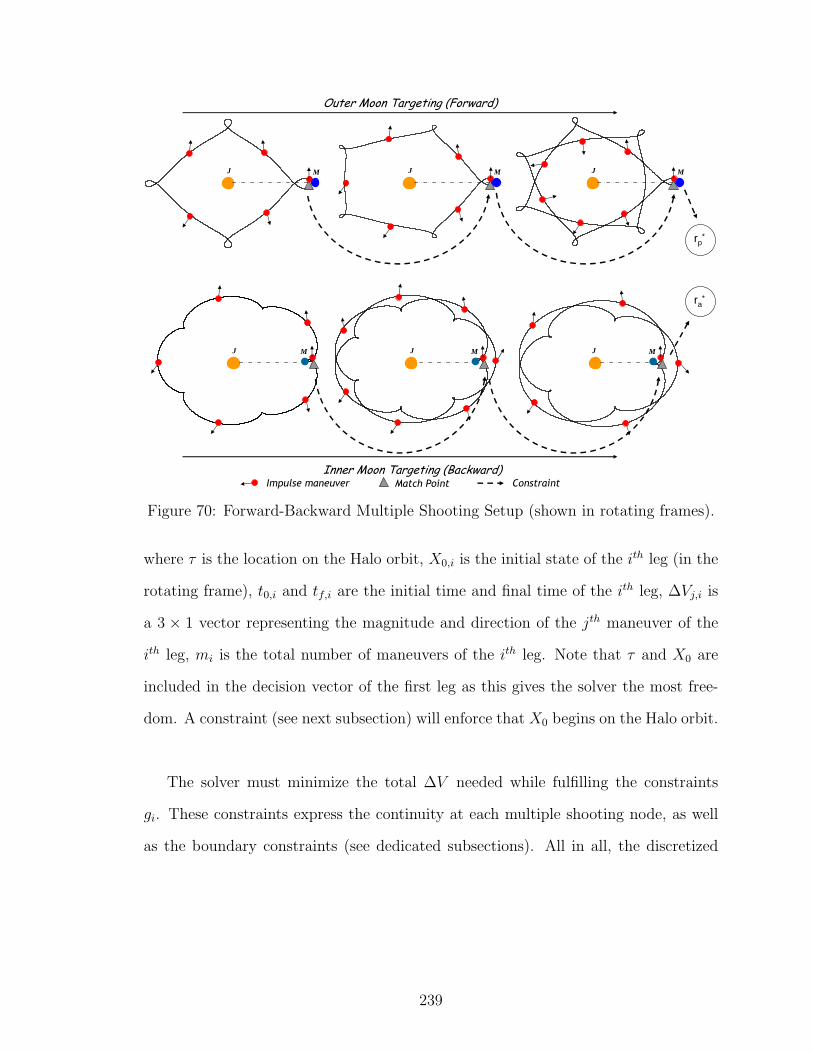
J M

Outer Moon Targeting (Forward)

rp*

J M J M

J M MJ MJ

ra*

Inner Moon Targeting (Backward)Impulse maneuver Match Point Constraint

Figure 70: Forward-Backward Multiple Shooting Setup (shown in rotating frames).

where τ is the location on the Halo orbit, X0,i is the initial state of the ith leg (in the

rotating frame), t0,i and tf,i are the initial time and final time of the ith leg, ∆Vj,i is

a 3 × 1 vector representing the magnitude and direction of the jth maneuver of the

ith leg, mi is the total number of maneuvers of the ith leg. Note that τ and X0 are

included in the decision vector of the first leg as this gives the solver the most free-

dom. A constraint (see next subsection) will enforce that X0 begins on the Halo orbit.

The solver must minimize the total ∆V needed while fulfilling the constraints

gi. These constraints express the continuity at each multiple shooting node, as well

as the boundary constraints (see dedicated subsections). All in all, the discretized

239

subproblem is mathematically formulated as follows:

minZ1,...,ZN

∑i

mi∑j=1

‖∆Vj,i‖

subject to

Ψ0(Z1) = 0

gi(Zi, Zi+1) = 0 for i = 1...n− 1

gn(Zn) = 0

(8.8)

A first guess is generated using the manifolds and resonant periodic orbits (at

appropriate energy levels) obtained with the method described in section 8.3. The

times and states of each node are therefore specified. In particular, a good initial guess

for X0,1 is found from applying from the (τ, ε) parameterization of the manifold of

Eq. (8.4a) and Eq. (8.4b). Thrust impulses are initialized to zero along the trajectory.

We use OPTIFOR to solve this very challenging multi-phase optimization prob-

lem. All the optimizations presented in this study are done using SNOPT and HDDP.

More details on the functions (propagation, constraints) characterizing the optimiza-

tion problem are given next.

8.4.1.3 Propagation Function

The propagation function is made of two parts: 1) the addition of the ∆V impulse to

the spacecraft velocity; 2) the numerical integration of the equations of motion of the

CR3BP in the inertial frame over the duration of one segment. A Runge-Kutta 7(8)

integrator is employed with an error tolerance of 10−12. In addition, recall that the

initial state parameters of the decision vector are defined in the rotating frame, thus

it is necessary to perform a rotation to the non-rotating frame at the beginning of

each leg. Lastly, note that we assume impulsive ∆V and therefore keep mass constant

across each ballistic segment.

240

OPTIFOR requires an accurate estimation of the State Transition Matrix of the

equations of motion (including state and time components). We compute these deriva-

tives via the complex-step differentiation method described in Chapter 4 and Ref. 155.

8.4.1.4 Initial Halo Boundary Condition

A boundary condition must be enforced to ensure that the departing point of each

moon-dominant phase lies on the corresponding nominal Halo orbit chosen for the

mission. Since the initial states are free and a point on the Halo orbit can be uniquely

identified by means of τ (see section 8.3), the initial boundary constraint Φ0 must be

written:

Ψ0 = X0,1(t0,1)−Xτ (τ) = 0 (8.9)

where Xτ (τ) is a generic point on the Halo orbit, and X0,1 are the initial states of

the first leg (part of the control vector Z1). We point out that ε is not part of the

constraint, which implies we target the pure Halo orbit and not the manifold state.

The small initial ∆V provides freedom for the solver to find the natural departure

along the manifold.

In practice, to avoid integrating the Halo orbit at every iteration (while calculat-

ing the boundary constraint), we perform a curve fit of the Halo orbit using a cubic

spline interpolation as a function of τ . At any location τ , nearly exact values for the

states (and the partial derivatives with respect to τ) can be then quickly retrieved

during the optimization process.

Note that the initial boundary constraint is required because the initial states

of the first leg X0,1 are free for improved flexibility. Other parameterizations could

sacrifice this extra freedom to avoid this extra constraint. For instance, to automat-

ically start on the Halo, X0,1 can be removed from the decision vector of the 1st leg

241

so that the starting conditions are only defined by X(τ). However, in that case, no

perturbation in the position eigenvector direction can be applied and the method of

section 8.3 cannot be directly used. Instead, it would be necessary to generate con-

tour maps where only the velocity is perturbed by epsilon in the unstable direction.

These newly-defined maps are more complex and do not present the nice linearity

seen in Figure 63, so finding empirical relationships is not straightforward. In such

a case, the resulting velocity perturbation would be used as the initial guess for the

first ∆V .

8.4.1.5 Final T-P Graph Constraint

The crucial question of the determination of the boundary condition for the forward-

backward patch point is discussed in this section. The method is similar to the one

described in Ref. 137 and relies on a new graphical tool, the Tisserand-Poincare (T-

P) graph, introduced by Campagnola and Russell.48 The overall principle is recalled

here. On the T-P Graph, level sets of constant Tisserand parameter are plotted in (ra,

rp) space where the Tisserand parameter is almost equivalent to the Jacobi constant

of the CR3BPc. During the resonance hopping transfer, the spacecraft moves along

the level sets of Tisserand curves. In fact, ballistic transfers are fixed in Jacobi con-

stant (and approximately fixed in the Tisserand parameter when evaluated far from

the minor body). The impulsive maneuvers allowed in our model are small enough

to not change the Jacobi constant to first order.

The intersection point between the Tisserand level sets of the trajectories associ-

ated with the two different moons is therefore the target patch point (see Figure 71).

cThe near equivalency is valid only when the Poincare section that generates the T-P graph isfar from the minor body.

242

rp

ra

Patch

point

CM2

CM1

Figure 71: Patch Point on the T-P Graph.

The target r∗a and r∗p are obtained by solving the system:CM1 = 2aM1

ra+rp+ 2√

2rarp(ra+rp)aM1

CM2 = 2aM2

ra+rp+ 2√

2rarp(ra+rp)aM2

(8.10)

where CM1 is the Jacobi constant of the forward trajectory, CM2 is the Jacobi constant

of the backward trajectory, aM1 is the semi-major axis of the first moon and aM2 is

the semi-major axis of the second moon. We call the pair (r∗a, r∗p) the solution of this

system. It follows that the T-P graph provides a simple way to calculate the patch

point (i.e. the planar orbit) that ballistically connects the forward-backward phases

of the trajectory. The forward phase targets r∗p and the backward phase targets r∗a.

Therefore, the final constraint of each phase is of the form:

g = rp/a − r∗p/a (8.11)

where rp/a is the final apse value of the current trajectory. The problem is thus reduced

to a one-dimensional targeting problem and the solution to the forward and backward

problems are uncoupled (to first order assuming the impulsive maneuvers do not

change the respective Jacobi constants). We are therefore able to break the original

problem at the patching point into two sub-problems, and each sub-problem can

be independently optimized (opening the possibility of parallel computation). This

approach is significantly easier than previous methods. Traditionally, one must target

the coupled six-states of an arbitrary non-optimal, switching orbit (the Hohmann

orbit in general).40 Another method is given in Ref. 102 where a ‘switching region’ is

243

introduced to give the approximate location in phase space where the switch occurs.

Note that the latter method is not able to define precisely the switching orbit to target.

Finally, it is emphasized that the optimization will inherently take advantage of the

perioidic orbit stable/unstable manifold dynamics. However, the tedious process of

generating manifolds and looking for intersections is not necessary in our approach.

8.4.2 End-to-End Patched Three-Body Optimization

The outer and inner moon portions of the transfer are patched together to form a

trajectory that begins at the Halo orbit of the outer moon and ends at the Halo

orbit of the inner moon. Ideally, the forward and backward parts of the trajectory

should patch perfectly, without the need to refine the trajectory. However, in prac-

tice, an end-to-end optimization step is required to obtain perfect continuity. One

reason is that the computations of ra and rp are approximate as they rely on two-

body theory, so a small error is introduced in the calculation of the patching point.

In addition, even if the thrust impulses are small, they generally modify the Jacobi

constant (Tisserand parameter), and this small change should formally be reflected

when the system of Eq. (8.10) is solved.

For achieving exact continuity, it is necessary to adjust the phase between the

inner moon and the outer moon at the time of intersection. The required phasing θ

of Europa with respect to Ganymede is given by the following relationship:

θ = arccos(R∗Gan ·R∗Eurr∗Ganr

∗Eur

) + wEurTOF (8.12)

where R∗Gan and R∗Eur are the position vectors of Ganymede and Europa at the patch

(when no initial phasing is taken into account), and TOF is the time of flight of the

whole trajectory. Finally, the solutions of the two portions of the last subsection are

combined and used as the initial guess for this step. Note that in our implementation

244

the solution of the backward phase must be reversed so that the whole trajectory can

be integrated forward.

Sometimes, the position and velocity z-components of the two portions differ sig-

nificantly (the out-of-plane components are not taken into account in the T-P graph

theory). When this happens, an intermediate step is added to re-optimize separately

one of the phases d to ensure continuity of the z-components with the other phase.

It is in fact more efficient to resolve the discontinuity when the phasing between the

moons is still free (the solver has more degrees of freedom).

8.4.3 Higher-Fidelity, Ephemeris-Based Optimization

The CR3BP and patched CR3BP models are convenient since they can offer dynam-

ical insight on the mechanisms of low-energy transport, while yielding good approxi-

mations to the motion in a multi-moon system. However, these three-body models are

ideal and do not reflect the true dynamics of the problem. It is therefore necessary to

transition the ideal model solution to a more realistic, ephemeris-based model. Sur-

prisingly, this final important step is not considered in most of the existing literature

applying dynamical system theory. Conventional wisdom suggest this final step is

tedious yet simple to converge and is generally left to the advanced stages of mission

design. While this mindset may be valid in the framework of patched conics, we find

that the final high fidelity transition step is far from trivial to achieve in the realm of

chaotic dynamics, high altitude gravity assists, and low energy resonant hopping.

To overcome this difficulty, a continuation method is employed to parametrically

change the solution from the patched three-body model to a four-body ephemeris-

based model. A similar method was implemented in Ref. 219 for obtaining solutions

dThe phase to be re-optimized can be chosen arbitrarily. It is recommented to optimize the phasewith the least number of resonances.

245

in higher-fidelity models. For any time, the states of the planet and the moons are

determined by a linear interpolation between the ideal model and ephemeris model

locations:

X(λ) = (1− λ)XCR3BP + λXephem (8.13)

where 0 ≤ λ ≤ 1, XCR3BP are the states given by the ideal model and Xephem are the

states of the ephemeris model. Starting at λ = 0, successive sub-problems are then

solved by slowly increasing the parameter λ, so that the model is slowly modified

from a patched circular, planar three-body model into a four-body ephemeris-based

model. When λ = 1, the last subproblem solved corresponds to the desired state

values X(λ = 1) = Xephem. This approach is robust and easy to implement, and

should work well since moon orbits are closely modeled by Keplerian motion.

In this step we emphasize that any ephemeris model can be considered. In this

paper, for simplicity we decide not to use published solar system ephemerides mainly

because the corresponding force and perturbation model is inconsistent with our four

body model. Instead, we generate a simplified and self-consistent ‘fake’ ephemeris

that takes only into account the simultaneous gravitational influences of the system

planet plus the two moons. This should produce results close to reality since any other

force is a minor perturbation. The equations of motion are numerically integrated

using an n-body propagator to obtain the states of the planet and the moons. The

initial conditions are derived from two-body motion and we subtract the motion of

the center of mass of the system from the integrated results so that the center of mass

appears stationary. In addition, we use cubic splines to interpolate the integration

data for specific times. Note that the epoch time must be chosen carefully so that the

phasing between the two moons (at least once over the interval) satisfies Eq. (8.12).

246

8.5 Numerical results

In this section, we demonstrate the efficiency of our method by computing several

optimal low-energy, resonant hopping transfers between planetary moons. This ex-

ample is chosen because the transfer between Ganymede and Europa is a common

benchmark problem studied by many authors,48,98,102,128 and this problem is relevant

in the context of future Jovian missions. Table 22 gives specific values for the CR3BP

parameters used in this paper for the Jupiter-Ganymede and Jupiter-Europa systems.

We provide solutions that both include Halo orbits as boundary conditions as well as

the simpler planet centric resonant orbits.

Table 22: Jupiter-Ganymede and Jupiter-Europa CR3BP parameters.

CR3BP Mass ratio Orbital Radius Orbital periodLU (km) TU (days)

Jupiter-Ganymede 7.8027 10−5 1.070339 106 7.154280561Jupiter-Europa 2.528 10−5 6.709 105 3.550439254

8.5.1 Pure Resonance Hopping Transfers

First, we do not consider Halo orbits in the transfer, so that the trajectories go from

a resonance close to Ganymede to a resonance close to Europa. Since our procedure

is systematic, we can perform a rudimentary ∆V vs flight time trade study to test

a variety of optimized resonant paths. The solver SNOPT is used here to perform

the optimizations. We select different combinations of the significant resonant orbits

given by the Keplerian Map (see Section 8.3.1) for Ganymede and Europa. The Jacobi

constants of the two portions of the trajectories are initially set to CGanymede = 3.0068

and CEuropa = 3.0024. These values are known, from previous numerical experiments,

to lead to feasible low-energy transfers.128 Furthermore, we seek energy levels that

are consistent with low-energy captures or escapes at the respective Moons. The

247

minimum energy level (maximum C) possible for escape or capture is of course the

energy level when Hill’s neck emerges as part of the zero velocity curves that separate

valid and forbidden regions.216,217 The initial and final resonances, 4 : 5 and 6 : 5,

respectively, are chosen because they can be reached by simply ‘falling off’ Halo orbits

close the moons.216

100 120 140 160 180 200 220 24040

60

80

100

120

140

160

180

Time of Flight (days)

∆V (

m/s

) 1

23 4

5

6 7

8 9

10 Pareto Front

Figure 72: Trajectory Scatter Plot for Ganymede-Europa transfer.

Table 23: Description of the different transfers.

# Resonant Path Resonant Path ∆V TOFGanymede Europa (m/s) (days)

1 4:5, 3:4, 5:7 7:5, 4:3, 9:7, 6:5 125.9 1192 4:5, 3:4, 5:7 7:5, 11:8, 9:7, 6:5 66.3 1443 4:5, 3:4, 5:7 7:5, 11:8, 4:3, 9:7, 6:5 59.5 158.54 4:5, 3:4, 5:7 7:5, 11:8, 4:3, 9:7, 5:4, 6:5 59.2 1775 4:5, 7:9, 3:4, 5:7 7:5, 11:8, 9:7, 6:5 64.3 1956 4:5, 7:9, 3:4, 5:7 7:5, 11:8, 4:3, 9:7, 6:5 56.5 2097 4:5, 7:9, 3:4, 5:7 7:5, 11:8, 4:3, 9:7, 5:4, 6:5 55.5 2278 4:5, 7:9, 3:4, 5:7 7:5, 4:3, 9:7, 6:5 110.2 1709 4:5, 7:9, 3:4, 5:7 7:5, 4:3, 9:7, 5:4, 6:5 112.7 18910 4:5, 3:4, 5:7 7:5, 4:3, 9:7, 6:5 178.2 149

The scatter plot of the results is shown in Figure 72 along with an approximate

Pareto Front. Table 23 details each resonant hopping sequence of this plot. The

248

last resonant orbits of the resonant path of each phase (5 : 7 and 7 : 5 respectively)

are only used as a guess of the patch point. This is possible because the switching

orbit occurs close to 5 : 7 and 7 : 5 (see right plot on Figure 76), but this is only a

coincidence due to the orbital characteristics of the Ganymede and Europa transfer

(it is generally not a : b then b : a).

Despite the high sensitivity of the problem, convergence is achieved for all tested

combinations, and the average computational time for each case is in the order of

two or three minutes using the Intel Fortran compiler and a 2.0 GHz processor (one

minute per phase approximately). Generating this set of solutions therefore demon-

strates that our approach is systematic, fast, and robust.

The theoretical minimum ∆V from V-infinity leveraging can be computed from

a quadrature.47 Using this equation, the minimum ∆V for a 4 : 5-to-6 : 5 transfer is

found to be 183 m/s. We can see that our method gives far lower ∆V . On our best

transfer (55 m/s), we get a 70 % reduction in ∆V compared to the best theoretical

∆V possible from the patched-conic based VILM strategy. In addition, comparison

of our results with those of a recent detailed study of VILM transfers40 shows that

our flight times are at the same order of magnitude.

These results suggest that the resonant paths from Ref. 40 are good initial paths

to examine. However, according to Ref. 47 and conventional wisdom, if the exact Vin-

finity leveraging (high-energy) solution is used as an initial guess for an optimizer,

then a nearby local minimum in the higher fidelity model will be found with similar

results. Instead, if a robust solver is used in conjunction with the periodic resonant or-

bits as an initial guess, then the low energy, low ∆V alternative solution can be found.

249

It is clear that solution 3 can be seen as a good compromise between fuel con-

sumption and time. For this transfer, there are two Ganymede flybys and four Europa

flybys. A total ∆V cost of 59.5 m/s is required and the total flight time is 158.5 days,

which is well within conceivable mission constraints. As a basis of comparison, it

takes up to 5 m/s just to navigate a flyby,237 so the ∆V cost is almost at the level

of statistical maneuvers. The corresponding entire trajectory of solution 3 is shown

with time histories of semi-major axis and apse distances in Figure 73 - Figure 75.

−1 −0.5 0 0.5 1

−0.8

−0.6

−0.4

−0.2

0

0.2

0.4

0.6

0.8

x (DU)

y (D

U)

Figure 73: Quasi-ballistic Ganymede-Europa transfer in the inertial reference frame.

0 20 40 60 80 100 120 140 1606.5

7

7.5

8

8.5

9

9.5

10

10.5x 10

5

Time (days)

(km

)

ra

arp

Figure 74: Periapsis, apoapsis, and semi-major axis time evolution of the quasi-ballistic transfer.

250

−1 −0.5 0 0.5 1−1

−0.8

−0.6

−0.4

−0.2

0

0.2

0.4

0.6

0.8

1

x (DU)

y (D

U)

−1.5 −1 −0.5 0 0.5 1 1.5−1.5

−1

−0.5

0

0.5

1

1.5

x (DU)

y (D

U)

Figure 75: Ganymede portion of the quasi-ballistic transfer in the rotating referenceframe of Ganymede (left). Europa portion of the quasi-ballistic transfer in the rotatingreference frame of Europa (right).

In particular, from Figure 74, we see that the semi-major axis is decreased se-

quentially, as expected. First, the trajectory gets its rp reduced with two flybys of

Ganymede. Then, the spacecraft passes naturally to the control of Europa and ac-

cordingly reduces its ra. Ref. 217 gives a high altitude closed periodic orbit at Europa

for a Jacobi constant of 3.0023 (ID 1486948), therefore our final resonance obtains an

energy value, C = 3.0024, that is consistent with loose capture around Europa. We

emphasize that the trajectory does include phasing and several fully integrated flybys

of both Ganymede and Europa. The data of this example are given in Appendix E.

Further insight of the dynamics is seen when plotting the spacecraft trajectory

on the T-P graph (see Figure 76). The spacecraft begins its transfer around the

center of the figure on a low-energy Ganymede Tisserand curve. The spacecraft has

its rp reduced via Ganymede gravity assists until it reaches the intersection with the

desired Europa Tisserand level set. Then the spacecraft falls under Europa’s influence

where its ra is decreased while its rp is approximately kept constant (according to the

level Tisserand curve). Overall, the transfer orbit scarcely deviating from curves of

constant Tisserand parameter, which validates the use of the T-P graph. In the right

plot of Figure 76, we can verify that the optimized switch point is very close to the

251

theoretical switching point predicted by the T-P graph theory (Eq. (8.10)). The 5 : 7

and 7 : 5 resonances of the initial Jacobi constants are also shown to point out that

the switch indeed occurs in their neighborhood, as expected.

ra (km)

r p (km

)

6 7 8 9 10 11 12

x 105

5

6

7

8

9

10

11

x 105

Ganymede Tisserand levelsEuropa Tisserand levelsGanymede transferEuropa transferPatching Point

4:5

3:4

6:5 9:7

4:3

11:8

ra (km)

r p (km

)

0.985 0.99 0.995 1 1.005 1.01 1.015 1.02 1.025

x 106

6.75

6.8

6.85

6.9

6.95

7

7.05

7.1

x 105

Ganymede Tisserand levelsEuropa Tisserand levelsOptimized Patching PointTheoretical Patching PointGanymede 5:7 resonanceEuropa 7:5 resonance

Figure 76: Left: T-P graph of the quasi-ballistic transfer. Right: Zoom of the T-Pgraph on the switching region.

8.5.2 Low-Thrust Resonance Hopping Transfer

Since the total ∆V ’s of the previous solutions are very low, we expect low-thrust

solutions to be feasible. To confirm this hypothesis, we intend in this subsection to

design a low-thrust trajectory for inter-moon transfers. Even if the current ESJM

baseline mission does not plan to use low-thrust propulsion, this is not an option to

be overlooked. The canceled JIMO mission included an ion engine for performing a

Jupiter tour,228 and there will be other outer planet missions in the future that might

reconsider low thrust.

We consider here that the spacecraft has a low-thrust engine with a specific impulse

Isp of 2000 s and a maximum thrust Tmax of 0.02 N. The initial mass of the spacecraft

is 1000 kg. Ten ∆V s per inertial revolution are included in the decision vector to

approximate the continuous control authority of low-thrust trajectories. In addition,

a constraint is added at each stage to enforce the limitation of the magnitude of the

impulse (see Eq. (5.9)).

252

−1 −0.5 0 0.5 1

−0.8

−0.6

−0.4

−0.2

0

0.2

0.4

0.6

0.8

x (DU)

y (D

U)

0 20 40 60 80 100 120 140 160 1800

0.005

0.01

0.015

0.02

0.025

Time (days)

Thr

ust (

N)

Figure 77: Inertial trajectory (left) and thrust profile (right) of the low-thrust, low-energy transfer.

The dimensionality of this problem is large, so we select our HDDP solver for the

optimization. We take the best resonant path found in the previous section (case 3

in Table 23), and the corresponding solution found in the previous section is given

to HDDP as an initial guess. It follows from the resonant path that the problem is

formulated with 8 phases. The initial guess is expected to be reasonably good since

low-thrust optimal solutions have been empirically determined to follow resonant

periodic orbits.262 Surprinsgly, even if the ∆V ’s are low, this initial guess is unfeasible

and violates a few stage constraints. The multicomplex-step differentiation described

in Chapter 4 is used to compute the first- and second-order derivatives required by

HDDP. Figure 77 shows the optimal solution found by HDDP. As expected, the

converged is bang-bang. The total accumulated ∆V required for this transfer is 22.2

m/s and the final mass is 998.86 kg (i.e. only 1.13 kg of propellant is required!).

8.5.3 Quasi-Ballistic Halo-to-Halo transfer

In this subsection, we use the complete procedure described in thid chapter to find

an optimal end-to-end trajectory from a Halo orbit of the L1 point of Ganymede to

a Halo orbit of the L2 point of Europa. The extra boundary constraints of the Halo

orbits make this problem much more challenging that that of the previous section.

253

The Jacobi constants of the Halo orbits and the two portions of the trajectories are

initially set to CGanymede = 3.0066 and CEuropa = 3.0024. These energy levels are

consistent with low-energy captures or escapes at the respective Moons. In addition,

these particular values are the result of some trial-and-error simulations to naturally

find a nearly-continuous match between the z-components of the two portions at the

patch point.

Unstable Manifold Type I 4:5 Resonance 3:4 Resonance

Stable Manifold Type II

6:5 Resonance 9:7 Resonance 4:3 Resonance 11:8 Resonance 7:5 Resonance

Figure 78: Orbits composing the initial guess of the transfer (rotating frames).

Table 24: Initial conditions (rotating frame) and characteristics of the Halo orbitsused in the transfer. Note y0 = 0, x0 = 0 and z0 = 0.

x0 (DU) z0 (DU) y0 (DU/TU) Period (TU) C (DU2/TU2)Halo 1 0.976829770381 0.006757550814 -0.033870558835 3.0136803932 3.0066Halo 2 1.011804392008 0.008754792713 0.035706638823 3.0645602543 3.0024

Table 25: Initial conditions and characteristics of the manifold trajectories shown inFigure 78.

τ ε Flight Time (TU) a (DU)e C (DU2/TU2)Manifold I + 4:5 res. 0.5 1.7 10−6 30.34682557231 0.8618 3.0066Manifold II + 6:5 res. 0.5 1.05 10−6 42.88481483746 1.1292 3.0024

eThe semi-major axis is computed far from the secondary body.

254

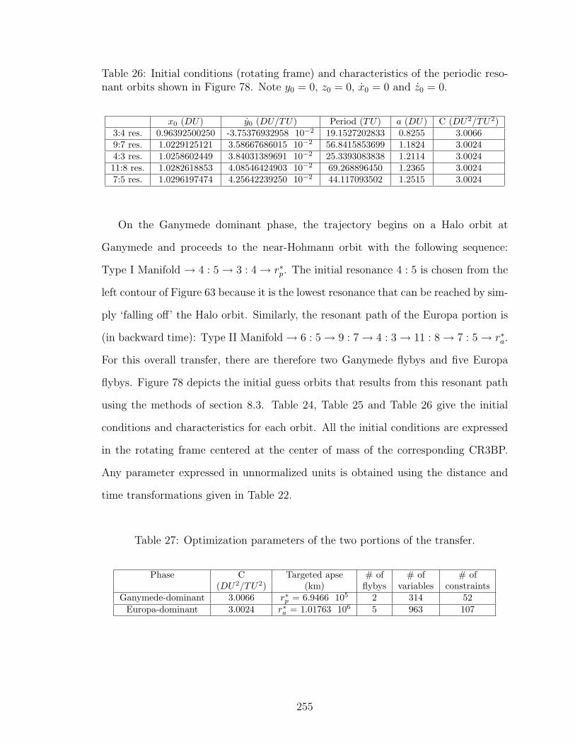
Table 26: Initial conditions (rotating frame) and characteristics of the periodic reso-nant orbits shown in Figure 78. Note y0 = 0, z0 = 0, x0 = 0 and z0 = 0.

x0 (DU) y0 (DU/TU) Period (TU) a (DU) C (DU2/TU2)3:4 res. 0.96392500250 -3.75376932958 10−2 19.1527202833 0.8255 3.00669:7 res. 1.0229125121 3.58667686015 10−2 56.8415853699 1.1824 3.00244:3 res. 1.0258602449 3.84031389691 10−2 25.3393083838 1.2114 3.002411:8 res. 1.0282618853 4.08546424903 10−2 69.268896450 1.2365 3.00247:5 res. 1.0296197474 4.25642239250 10−2 44.117093502 1.2515 3.0024

On the Ganymede dominant phase, the trajectory begins on a Halo orbit at

Ganymede and proceeds to the near-Hohmann orbit with the following sequence:

Type I Manifold → 4 : 5→ 3 : 4→ r∗p. The initial resonance 4 : 5 is chosen from the

left contour of Figure 63 because it is the lowest resonance that can be reached by sim-

ply ‘falling off’ the Halo orbit. Similarly, the resonant path of the Europa portion is

(in backward time): Type II Manifold→ 6 : 5→ 9 : 7→ 4 : 3→ 11 : 8→ 7 : 5→ r∗a.

For this overall transfer, there are therefore two Ganymede flybys and five Europa

flybys. Figure 78 depicts the initial guess orbits that results from this resonant path

using the methods of section 8.3. Table 24, Table 25 and Table 26 give the initial

conditions and characteristics for each orbit. All the initial conditions are expressed

in the rotating frame centered at the center of mass of the corresponding CR3BP.

Any parameter expressed in unnormalized units is obtained using the distance and

time transformations given in Table 22.

Table 27: Optimization parameters of the two portions of the transfer.

Phase C Targeted apse # of # of # of(DU2/TU2) (km) flybys variables constraints

Ganymede-dominant 3.0066 r∗p = 6.9466 105 2 314 52Europa-dominant 3.0024 r∗a = 1.01763 106 5 963 107

255

In addition, Table 27 summarizes several parameters that characterize the opti-

mization procedure in each CR3BP portion of the transfer. Throughout the trajec-

tory, eight ∆V s per inertial revolution are included in the decision vector, which leads

to 314 control variables in the Ganymede-dominant phase and 963 control variables

in the Europa-dominant phase. SNOPT is used to solve the resulting problems.

Figure 79 (on the right) shows the difference between the CR3BP and the four-

body ephemeris model for the orbital radii of Ganymede and Europa. We can see in

the ephemeris model short-term sinusoidal variations of increasing amplitude. The

initial conditions used for the four body integration of the ephemeris are presented

in Table 28.

Table 28: Initial conditions (inertial frame) in the generation of the ephemeris model.

Position (km) Velocity (km/s)Jupiter [−13.2225, 10.6217, 0]

[−0.2176 10−3,−0.2708 10−3, 0

]Ganymede

[1.07026 106, 0, 0

][0, 10.8790, 0]

Europa[5.2303 105,−4.2015 105, 0

][8.6057, 10.7129, 0]

0 200 400 600 800 1000−1.5

−1

−0.5

0

0.5

1

1.5x 10

4

Time (days)

Diff

eren

ce in

rad

ius

(km

)

GanymedeEuropa

−150 −100 −50 0 50 100 150−150

−100

−50

0

50

100

150

x (km)

y (k

m)

Four−Body Ephemeris ModelThree−Body Model (Jupiter−Ganymede)

Figure 79: Comparisons between the CR3BP and four-body ephemeris models. Left:difference in Ganymede and Europa orbital radii. Right: Jupiter positions in the twomodels.

256

Table 29 summarizes the results for this resonant hopping sequence for each model

considered. The total ∆V and total time of flight of the trajectories are given, as well

as the approximate computational times and function calls for the solutions of each

fidelity. Computations are performed using the Intel Fortran compiler (with speed

optimization settings) and a 2.0 GHz processor. All constraints are enforced with a

normalized tolerance of 10−8, which corresponds to position and velocity discontinu-

ities of around 10 m and 0.1 mm/s respectively. Targeting such a high tolerance is

facilitated by the robust multi-shooting implementation.

Table 29: Optimization Results for each model.

Model ∆V TOF # of Computational # ofruns time function calls

Independent CR3BPs 40.5 m/s 204.4 days 2 50 min 2200Patched CR3BP 42.2 m/s 204.3 days 1 10 min 370

Ephemeris Four-Body 54.7 m/s 204.5 days 1000 1 week ∼ 100,000

We can see that the total ∆V is extremely low, and similarly across model fidelity.

Our objective to find a quasi-ballistic transfer is therefore achieved. In fact, the deter-

ministic ∆V of ∼ 50 m/s is on the same order of magnitude that is typically budgeted

for statistical ∆V s required to correct gravity assisted flyby errors (7 flybys × ∼ 5

m/s/flyby = ∼ 35 m/s). The lowest ∆V corresponds to the independent CR3BPs,

but the trajectory is not fully continuous at the patch point. For the patched CR3BP

model, the total ∆V cost of 42.2 m/s is required and the total flight time is 204.3

days. In addition to this low ∆V , the time of flight is also favorable compared to

typical results involving resonant gravity assists and invariant manifolds.88

Interestingly, the results in the ephemeris model are very similar with those of

the patched CR3BP model. The ∆V is slightly increased and the time of flight is

257

almost identical. However, the continuation method that characterizes this step is ex-

tremely time consuming: one full week of computations is needed to transition to the

ephemeris model. In fact, because of the high sensitivity of the problem, a small vari-

ation of 10−2 for λ is necessary to ensure convergence, which leads to a total of 1000

optimization runs that must be performed in serial. We envision improvements that

will likely reduce the number of required optimizations, including predictor-corrector

methods that exploit the analytic sensitivity of the solution with respect to λ. We

leave this and other ideas as future work.

−1 −0.5 0 0.5 1

−0.8

−0.6

−0.4

−0.2

0

0.2

0.4

0.6

0.8

x (DU)

y (D

U)

Figure 80: Trajectory from Ganymede to Europa in inertial frame (patched CR3BPmodel).

0 50 100 150 200 2506.5

7

7.5

8

8.5

9

9.5

10

10.5x 10

5

Time (days)

(km

)

ra

arp

Ganymede Flyby 1

Ganymede Flyby 2

EuropaFlyby 1

EuropaFlyby 2

EuropaFlyby 3

EuropaFlyby 4

EuropaFlyby 5

Figure 81: Time history of semi-major axis, periapsis and apoapsis of the trajectory(patched CR3BP model).

258

−1 −0.5 0 0.5 1−1

−0.8

−0.6

−0.4

−0.2

0

0.2

0.4

0.6

0.8

1

x (DU)

y (D

U)

0.9 0.92 0.94 0.96 0.98 1−0.06

−0.04

−0.02

0

0.02

0.04

0.06

x (DU)

y (D

U)

Figure 82: Left: Ganymede-dominant phase in rotating frame. Right: Zoom in onGanymede flybys.

−1.5 −1 −0.5 0 0.5 1 1.5−1.5

−1

−0.5

0

0.5

1

1.5

x (DU)

y (D

U)

1 1.02 1.04 1.06 1.08−0.04

−0.03

−0.02

−0.01

0

0.01

0.02

0.03

0.04

0.05

x (DU)

y (D

U)

Figure 83: Left: Europa-dominant phase in rotating frame. Right: Zoom in onEuropa flybys.

The trajectory in the patched CR3BP model, along with with time histories of

semi-major axis and apse distances, are shown from Figure 80 to Figure 83. The

zooms on the flybys show that the obtained trajectory is continuous at the nodes of

the multiple shooting formulation. In addition, Figure 84 and Figure 85 show the

characteristics of the trajectory in our four-body ephemeris model. The left part of

Figure 85 gives the time history of the associated ∆V s and confirms that the trajec-

tory is mainly ballistic with a few number of impulses. Combining the information

in the two plots of Figure 85, we can deduce that there are three main impulses

required and two of them are located near the first and last flybys. We emphasize

that this trajectory is three-dimensional, includes phasing and several fully integrated

259

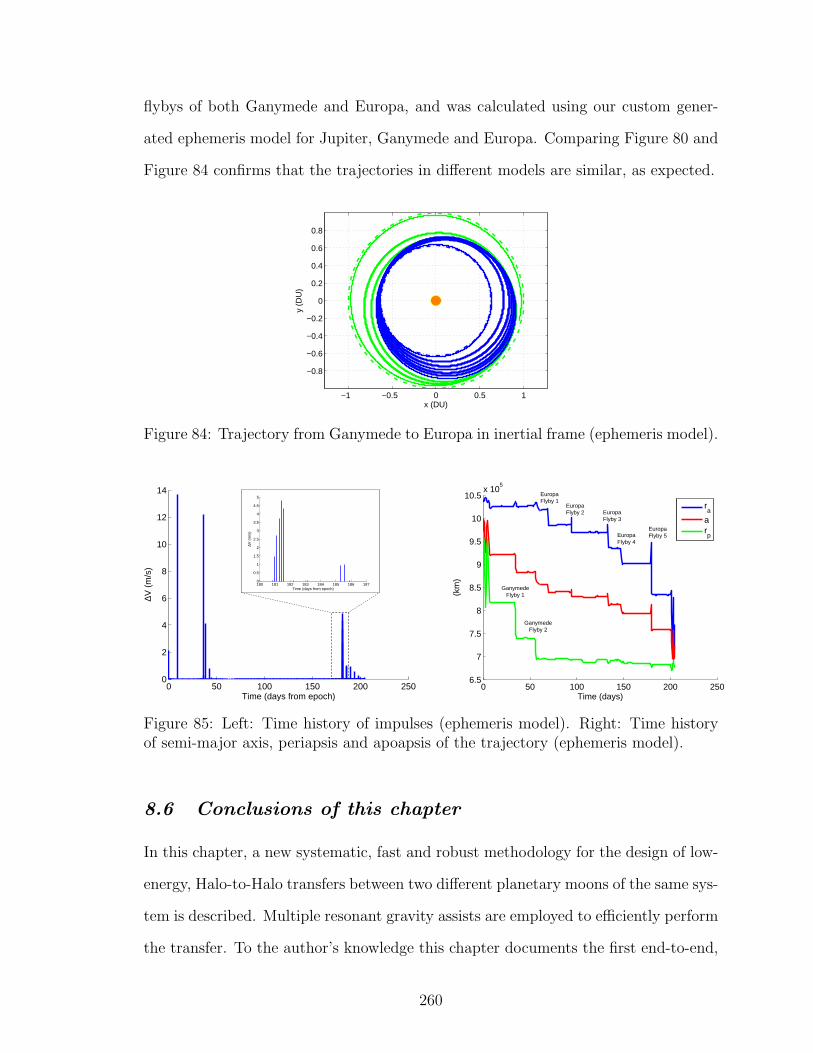
flybys of both Ganymede and Europa, and was calculated using our custom gener-

ated ephemeris model for Jupiter, Ganymede and Europa. Comparing Figure 80 and

Figure 84 confirms that the trajectories in different models are similar, as expected.

−1 −0.5 0 0.5 1

−0.8

−0.6

−0.4

−0.2

0

0.2

0.4

0.6

0.8

x (DU)

y (D

U)

Figure 84: Trajectory from Ganymede to Europa in inertial frame (ephemeris model).

0 50 100 150 200 2500

2

4

6

8

10

12

14


∆V (

m/s

)

180 181 182 183 184 185 186 1870

0.5

1

1.5

2

2.5

3

3.5

4

4.5

5


∆V (

m/s

)

0 50 100 150 200 2506.5

7

7.5

8

8.5

9

9.5

10

10.5x 10

5

Time (days)

(km

)

ra

arp

Ganymede Flyby 1

Ganymede Flyby 2

EuropaFlyby 1

EuropaFlyby 2 Europa

Flyby 3

EuropaFlyby 4

EuropaFlyby 5

Figure 85: Left: Time history of impulses (ephemeris model). Right: Time historyof semi-major axis, periapsis and apoapsis of the trajectory (ephemeris model).


In this chapter, a new systematic, fast and robust methodology for the design of low-

energy, Halo-to-Halo transfers between two different planetary moons of the same sys-

tem is described. Multiple resonant gravity assists are employed to efficiently perform

the transfer. To the author’s knowledge this chapter documents the first end-to-end,

260

near-ballistic transfer in any continuous force model that connects loosely captured

states at two different planetary moons. In addition, with a simple non-exhaustive

search, we are able to produce families of fuel-time Pareto optimized trajectory solu-

tions between close resonant orbits of Ganymede and Europa. A low-thrust trajectory

is also found to perform this type of resonant hopping transfer.

Our approach combines dynamical systems theory with optimal control tech-

niques. A first guess solution that takes advantage of the inherent dynamics of the

multi-body system is found using initial conditions of invariant manifolds and unsta-

ble resonant periodic orbits. An empirical relationship that maps reachable orbits

to/from Halos is developed to assist the process. The optimization is then performed

in models of increasing complexity using a direct multiple shooting strategy. For

evaluation in an ephemeris model, a robust continuation method is implemented. We

show that the formulated method can deliver an efficient quasi-ballistic solution for

a transfer between Ganymede and Europa. Notably, for this planetary moon system,

our analysis suggests that the solution in the custom four body ephemeris model does

not differ significantly from the one in the patched three-body model. However, we

emphasize that achieving the final ephemeris model solution is far from trivial and

has received little attention in the literature.

In addition, a by-product of this work is a deeper understanding of the dynamic

structure of resonance passes in the three body problem. We introduce the concept

of significant resonant transitions and explain why an efficient trajectory is likely to

cross them. The accuracy of the analytical Keplerian Map to approximate three-body

motion is also characterized in detail for the first time.

The multi-body resonant hopping technique is demonstrated as a promising and

261

advantageous alternative to the conventional patched conic methods. Overall, this

work can be seen as the next step in the direction towards the automated design of

satellite tours using multi-body dynamics.

262

CHAPTER IX

CONCLUSIONS

9.1 Dissertation Summary and Major Contributions

This dissertation deals with the optimal control problem of low-thrust trajectories

in multi-body environments. Considering these types of trajectories is necessary to

design ambitious fuel-efficient exploration missions of the solar system. This research

focuses mainly on three aspects: 1) development of robust optimization techniques

to solve challenging low-thrust problems ; 2) representation of low-thrust trajectories

with varying models of fidelity; and 3) combination of the developed optimization

methods with dynamical systems theory to compute low-energy inter-moon transfers.

First, the formulation of the low-thrust optimal control problem is introduced.

It is shown that our problem can be described as a discrete multi-phase problem

characterized by a set of ‘building block’ functions. The building blocks can de-

fine propagation models, constraints, costs or events associated to the corresponding

phase. This general trajectory paradigm allows us to accommodate a variety of mis-

sion scenarios with multiple planetary encounters. A unified optimization framework

OPTIFOR is developed to solve the resulting trajectory optimization problems. In-

terfaces to state-of-the-art NLP solvers SNOPT and IPOPT are included.

Then a new, robust Hybrid Differential Dynamic Programming (HDDP) algo-

rithm is presented to solve the large-scale optimal control problems that can arise

from low-thrust trajectories. The algorithm combines the conventional Differential

263

Dynamic Programming with nonlinear programming techniques (Lagrange multipli-

ers, trust-region, range-space method) to increase robustness and handle constraints.

The main steps of the algorithm are described in details. An important contribu-

tion of this thesis is that HDDP can handle multi-phase optimal control problems.

In addition, HDDP allows for a decoupling of the dynamics (state equations and

first- and second-order state transition matrices) from the optimization, as opposed

to other DDP variants. We emphasize that HDDP does not suffer from the ’curse

of dimensionality’ since large dimensioned problems are reduced to successive small

dimensioned subproblems. The algorithm is validated on a simple quadratic problem

with linear constraints showing global convergence in one iteration.

Crucial to any optimization procedure is the generation of the sensitivities with re-

spect to the variables of the system. Many applications in scientific computing require

higher order derivatives. In the context of trajectory optimization, these derivatives

are often tedious and cumbersome to estimate analytically, especially when complex

multi-body dynamics are considered. An innovative multicomplex-step differentiation

method is therefore derived to compute automatically first- and higher-order deriva-

tives. A couple of examples demonstrate that our method tends to perform well in

comparison with existing automatic differentiation tools. Note that a multicomplex

differentiation tool based on the method described here is available by request.

The developed optimization techniques are the first fundamental ’bricks’ neces-

sary to solve low-thrust problems. The next step is to implement different models to

represent low-thrust trajectories and their associated events. Emphasis is given on an-

alytical expressions to speed up the optimization of the corresponding trajectories. In

264

particular, we show that taking advantage of the well-known analytic partial deriva-

tives (up to second order) of Keplerian motion enables considerably faster computa-

tions compared to traditional formulations based on expensive numerical integrations.

In the same spirit, we then study exact, closed-form expressions of the so-called

Stark problem. This model allows us to parameterize the low-thrust problem by sub-

dividing the trajectory into two-body segments subjected to Newtonian gravitation

plus an additional uniform force of constant magnitude and direction. Compared to

existing analytic methods, this Stark model can take into account more accurately

the effect of thrusting and the full dynamics of the problem, at the expense of a

slight speed overload. First, all the general types of solutions, expressed in terms of

elliptic integrals, are described in details. Then a state-of-the-art optimization solver

specially tailored to exploit the structure of the problem is used to take advantage

of those closed-form solutions. Preliminary numerical results compared to existing

algorithms show the speed and accuracy advantages of this approach.

All our optimization and modeling techniques are then tested on several numer-

ical examples. Our in-house HDDP solver is confirmed to be robust and is able to

handle many encounter events. We also show that the HDDP solution can be used

as an initial guess for an indirect method that converges to the exact optimal solution.

Finally, we rely on all our developed techniques to generate low-energy inter-moon

trajectories with multiple resonant gravity assists (‘resonance hopping’). Using in-

sight from dynamical systems theory, we can generate good initial guesses to exploit

the chaotic nature of these systems. As a by-product, we perform a detailed study on

the accuracy of the Keplerian Map and interesting transition properties between Halo

265

and unstable resonant orbits are found. Special emphasis is also given to the reso-

nance transition mechanism through which a spacecraft hops from one resonant orbit

to another. With a simple non-exhaustive search, we produce families of fuel-time

Pareto optimized trajectory solutions between Ganymede and Europa. A resonant

hopping low-thrust transfer is also generated. Finally, low-energy, Halo-to-Halo trans-

fers between two different planetary moons of the same system are computed. It is

believed that this thesis documents the first end-to-end, near-ballistic transfer in any

continuous force model that connects loosely captured states at two different plane-

tary moons.

Robustness

HDDP (Chapter 3)

Multi-Phase Formulation (Chapter 2)

Exact Second-Order Derivatives (Chapter 4 & 5)

SpeedKepler Model (Chapter 5)

Stark Model (Chapter 6)Accuracy

High-Fidelity Dynamics (Chapter 5)

Flexibility

Generic Problem Formulation via Buidling Blocks (Chapter 2)

Automatic Derivatives via MultiComplex(Chapter 4)

Indirect Formulation (Chapter 2)

Figure 86: Improvements from the developed techniques of the thesis.

In summary, unique techniques are developed in this thesis to handle low-thrust

problems in multi-body dynamics. We believe that these techniques are true enablers

266

to solve some of the challenging problems facing a new era of robotic and human space

exploration. Recalling the four algorithm figures of merit described in section 1.3, Fig-

ure 86 shows the main criterion and the contributions from each developed technique.

It is also important to underline that many original concepts and ideas of this

thesis are independent from the specific low-thrust application. Many of the meth-

ods are stand-alone and can be used in a broad variety of science and engineering

applications (HDDP, OPTIFOR, Multicomplex, Stark).

9.2 Directions for Future work

While the practical results of the proposed methodology are very encouraging, there

is always room for improvement. Some possible aspects worthy of further investiga-

tion are presented below.

HDDP:

• Testing: Since our HDDP algorithm has been implemented only recently, con-

tinued testing and improvements will be necessary. Also, continued usage is

expected to reveal bottlenecks, either in the implementation or in the underly-

ing mathematical algorithm, and might raise interesting research questions.

• Incorporation of the null-space approach to enforce the constraints at each

quadratic programming subproblem (see section 3.3.3.1).

• Heuristics to find good tuning parameters for a wide range of problems in order

to improve robustness.

• Implementation of Quasi-Newton approximations of the Hessians to reduce com-

putational time.

267

Multicomplex-step differentiation:

• Efficient Matlab implementation.

• Parallelization of the computation of derivatives. Like Finite Differencing, the

multicomplex approach is inherently parallelizable.

Modeling:

• Indirect three-body formulation: the HDDP solution could then be used to find

exact optimal solutions in the CR3BP.

• Capability to change reference frames between phases, so that integrated flybys

can be modeled.

• Derivation of the analytical first- and second-order STMs of the three-dimensional

Stark problem (only the derivatives of the planar Stark problem have been de-

rived for this thesis).

Inter-Moon Transfers:

• For a more realistic and practical model, the radiation dose received by the

spacecraft should be taken into account in the optimization as well because

strong radiation background in the vicinity of Jupiter can decrease the dura-

bility of onboard electronics. In addition, the radiation dose plays a role when

comparing different options, especially when the transfer times and perijove pas-

sages vary significantly. To that end, using a simplified radiation model,120,124

an extra constraint on the maximum radiation dose allowed could be added in

Eq. (8.8), or the total radiation dose of the transfer could be included in the

objective function.

268

• Application of the methodology to a wider spectrum of problems. Other prob-

lems of interest include Callisto-Ganymede transfers and tours in other gas giant

systems such as Uranus or Saturn. For the moment, the methodology is limited

to two moons only, but we intend to extend it to specify intermediate moons as

well.

269

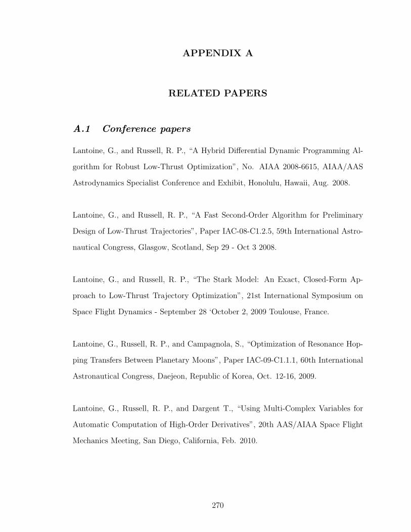
APPENDIX A

RELATED PAPERS

A.1 Conference papers

Lantoine, G., and Russell, R. P., “A Hybrid Differential Dynamic Programming Al-

gorithm for Robust Low-Thrust Optimization”, No. AIAA 2008-6615, AIAA/AAS

Astrodynamics Specialist Conference and Exhibit, Honolulu, Hawaii, Aug. 2008.

Lantoine, G., and Russell, R. P., “A Fast Second-Order Algorithm for Preliminary

Design of Low-Thrust Trajectories”, Paper IAC-08-C1.2.5, 59th International Astro-

nautical Congress, Glasgow, Scotland, Sep 29 - Oct 3 2008.

Lantoine, G., and Russell, R. P., “The Stark Model: An Exact, Closed-Form Ap-

proach to Low-Thrust Trajectory Optimization”, 21st International Symposium on

Space Flight Dynamics - September 28 ‘October 2, 2009 Toulouse, France.

Lantoine, G., Russell, R. P., and Campagnola, S., “Optimization of Resonance Hop-

ping Transfers Between Planetary Moons”, Paper IAC-09-C1.1.1, 60th International

Astronautical Congress, Daejeon, Republic of Korea, Oct. 12-16, 2009.

Lantoine, G., Russell, R. P., and Dargent T., “Using Multi-Complex Variables for

Automatic Computation of High-Order Derivatives”, 20th AAS/AIAA Space Flight

Mechanics Meeting, San Diego, California, Feb. 2010.

270

Lantoine, G., Russell, R. P., “Near-Ballistic Halo-to-Halo Transfers Between Plane-

tary Moons”, George H. Born Symposium, AAS, Boulder, CO, May 2010.

Russell, R. P., Lantoine, G., “Relative Motion and Optimal Control in Arbitrary

Fields: Application at Deimos”, Paper AAS 10-313, Kyle T. Alfriend Astrodynamics

Symposium, AAS, Monterey, CA, May 2010.

Lantoine, G., Russell, R. P., “A Unified Framework for Robust Optimization of In-

terplanetary Trajectories”, Paper AIAA-2010-7828, AAS/AIAA Astrodynamics Spe-

cialist Conference and Exhibit, Toronto, Canada, Aug 2010.

A.2 Journal papers

A.2.1 Accepted

Lantoine, G., Russell, R. P., Campagnola, S., “Optimization of Low-Energy Resonant

Hopping Transfers between Planetary Moons”, Acta Astronautica, (accepted Sept

2010).

A.2.2 Revisions being Processed

Lantoine, G., Russell, R. P., “Complete, Closed-Form Solutions of the Stark Prob-

lem”, Celestial Mechanics and Dynamical Astronomy, (accepted Nov 2010).

A.2.3 In review

Lantoine, G., Russell, R. P., “Near-Ballistic Halo-to-Halo Transfers Between Plane-

tary Moons”, Journal of the Astronautical Sciences.

Russell, R. P., Lantoine, G., “Relative Motion and Optimal Control in Arbitrary

Fields: Application at Deimos”, Journal of the Astronautical Sciences.

271

APPENDIX B

PROOFS OF SOME MULTICOMPLEX PROPERTIES

B.1 Matrix representation of multicomplex numbers

We give here the proof of Theorem 1. Let z = z1 + z2in be an element in Cn. First,

by quickly extending the proof of theorem 28.2 in the book of Price,198 we can say

that the set of 2× 2 multicomplex matrices of order n− 1 of the form

M(z) =

z1 −z2

z2 z1

= z1

1 0

0 1

+ z2

0 −1

1 0

(B.1)

is an isomorphism. In fact, clearly the 0 and identity matrix are of this form. Also

the sum and difference of matrices are of this form as well. Regarding the product of

matrices, we can readily see thatz1 −z2

z2 z1

w1 −w2

w2 w1

=

z1w1 − z2w2 z1w2 + z2w1

−(z1w2 + z2w1) z1w1 − z2w2

(B.2)

which is also of this form.

Next, the result of the theorem can be deduced by recurrence: z1 is equiv-

alent to

z11 −z12

z12 z11

. In the same way, z2 is equivalent to

z21 −z22

z22 z21

. In-

corporating these isomorphisms into Eq. (B.1), we can say that z is equivalent to

z11 −z12 −z21 z22

z12 z11 −z22 −z21

z21 −z22 z11 −z12

z22 z21 z12 z11

.

272

The theorem is then proven by repeating the same operation until a real matrix

is recovered. Note that by stopping one step before, we can represent multicomplex

numbers by complex matrices as well.

B.2 Divisors of zero of multicomplex numbers

Let the sets

Dk,1 = (z1 + z2in)ek,1/(z1 + z2in) ∈ Cn

Dk,2 = (z1 + z2in)ek,2/(z1 + z2in) ∈ Cn (B.3)

where ek,1 = 1+ikik+1

2, ek,2 = 1−ikik+1

2for k = 1, ..., n−1 are idempotents elements in Cn.

From Price,198 we can state that two elements in Cn are divisors of zero if and

only if one is Dk,1 − 0 and the other is in Dk,2 − 0 for any k = 1, ..., n− 1.

273

APPENDIX C

INTERACTIVE VISUALIZATION CAPABILITY

Trajectory optimization should include an interactive visualization capability to speed

up the development process of the optimization algorithm. Indeed, a graphics rep-

resentation of the trajectory at runtime provides an immediate visual feedback that

gives information on the rate of convergence or warns the user of input errors.

There are many graphics libraries available, but none were capable of support-

ing our custom needs.. Of course, some commercial packages would suffice, but cost

and license maintenance is an unwelcomed issue. So VISFOR was born. VISFOR

stands for Visual Interactive Simulation in FORtran. It is a powerful general-purpose

OpenGL graphics library written in Fortran and it is particularly suited for parallel,

interactive visualization of numerical simulations on desktop systems. VISFOR is

totally Fortran 9x-based, eliminating the need to resort to compiler-specific features,

mixed-language programming or low-level API calls. The library consists of around

7,000 lines of code, excluding specific OpenGL library interfaces.

Real-time interactive plotting is achieved through a parallel simulation-driven ar-

chitecture. At least one processor is in charge of the simulation (trajectory opti-

mization in our case). Another processor is responsible for the visualization. The

simulation provides a list of entities to be visualized, and this list can then be dis-

played asynchronously by the visualization engine.

A screenshot of VISFOR is given in Figure 88. Note that the windows layout and

274

Figure 87: VISFOR architecture.

content can be entirely customized easily.

Figure 88: VISFOR screenshot.

275

APPENDIX D

KICK FUNCTION AND APSE TRANSFORMATIONS IN

THE CR3BP

D.1 Kick Function at Apoapsis

At apoapsis of the trajectory, the kick function is given by:

f = − 1√p

∫ 2π

0

{[(r(ν)

r2(ν)

)3

− 1

]sin(θ(ν))

}dν (D.1)

where p = a(1− e2), r = p1+e cos ν

, r2 =√

1 + r2 − 2r cos θ,

E = 2 arctan(tan(ν2

)√1− e1 + e

), t = a

32 (E − e sinE − π), θ = w − π + ν − t.

Notations consistent with Ref. 212 are adopted and we assume µ = 1. Here ν is

the true anomaly of the trajectory.

D.2 Apsis Transformation to the Rotating Frame

Let w, a, C (Jacobi constant) given. Assume that the flyby is at periapsis (modify-

ing the equations for the apoapsis case is straightforward). We want to deduce the

corresponding state in rotating frame. First we compute the eccentricity from the

well-known expression of the Jacobi constant in function of a and e:212

C =1

a+ 2√a(1− e2)⇒ e =

√1− 1

4a

(C − 1

a

)2

(D.2)

Since we are at periapsis at an angle w with respect to the secondary body, the

position vector is:

R =

cosw − sinw

sinw cosw

rp

0

(D.3)

276

where rp = a(1− e). From the energy equation, the norm of the inertial velocity is:

v =

√2

(1

rp− 1

2a

)(D.4)

After rotating the velocity and going from inertial to rotating coordinates, we get:

V =

cosw − sinw

sinw cosw

0

v

+

0 1

−1 0

R (D.5)

277

APPENDIX E

RESONANT HOPPING TRANSFER DATA

We give here the solution vectors and the numerical data of the example given in

Section 8.5.

µGanymede = 7.802E−5.

dGanymede = 1070.4E3 km (orbital radius of Ganymede).

Initial inertial angle of Ganymede: 0o.

µEuropa = 2.523E−5.

dEuropa = 670.9E3 km (orbital radius of Europa).

Initial inertial angle of Ganymede: 319.5o.

The scaling of the variables of the solution vectors is given by:

position : 1070.4E3 km

velocity: 10.880850460047206 km/s

impulse: 1 m/s

time: 27.326295350266523 h

In order to preserve the dynamics of the CR3BP, we note that the origin is the

barycenter of the Jupiter-moon system and therefore Jupiter instantaneously changes

positions (albeit only on the order of 100 km) at the time of the switching orbit.

In the following, we give the solution vector for each leg in the same format as

Eq. (8.7), and a mesh vector corresponding on the time of the nodes of each leg:

tnode(j) = t0 +Kmesh(j)(tf − t0).

278

Ganymede portion of the trajectory:Leg 1:

Kmesh,1 = [0.0, 0.1, 0.3, 0.5, 0.7, 0.9, 1.0].

XLeg,1 =

0.971772553135740

2.000000000000000E − 003

−1.999999999940707E − 003

0.939663097665845

0.200000000000000

26.1383793256402

1.902195705689637E − 002

1.000000000000000E − 007

1.000000000000000E − 007

−2.46632086189342

1.04434783719898

−2.30313426639315

1.49055001006334

−2.07021545306293

1.81924488912533

−1.71199873686942

2.00562269946983

−1.28461657105624

.

Leg 2:

Kmesh,2 = [0.0, 0.125, 0.375, 0.625, 0.875, 1.0].

XLeg,2 =

0.963990317420658

1.179025646459924E − 002

−4.609328129500286E − 002

0.933124288254507

26.1383783256402

44.9895122805651

0.207999275978586

1.000000000000000E − 007

2.33960661397638

−1.47296105762402

2.07466654723355

−1.31718799713102

1.82070893670085

−1.15370667342255

1.58459650285961

−0.961187745920894

.

Leg 3:

Kmesh,3 = [0.0, 2.0].

XLeg,3 =

0.964061970680151

2.964154139140900E − 002

−3.805450663291127E − 002

0.917102399680224

44.9895132805651

47.2652495497626

1.14499708615006

−0.564503829255398

.

Europa portion of the trajectory (back-ward):Leg 1:

Kmesh,1 = [0.0, 0.1, 0.3, 0.5, 0.7, 0.9, 1.0].

XLeg,1 =

0.637781768756313

8.245934717884093E − 004

1.837411622748608E − 003

1.33077383729167

−7.437538661470156E − 002

−18.9972008288828

6.686944949979871E − 002

5.947036534038835E − 002

0.585729786148636

0.627291615239714

0.613082784861262

0.574344583252040

0.637785951527150

0.516755809028575

0.662349458231789

0.457346890540265

0.684858646978116

0.397312365752788

.

Leg 2:

Kmesh,2 = [0.0, 0.07142, 0.214285, 0.357142, 0.5,

0.642857, 0.78571, 0.92857, 1.0].

XLeg,2 =

0.638958805538506

1.071722538262295E − 002

−1.886141681665743E − 002

1.32393470040639

−18.9972018288828

−47.1751636470926

0.173781744405468

4.492524679035975E − 002

1.19850268950068

0.127589184909997

1.18393242448054

0.121502952758578

1.17106824105797

0.113850880596218

1.15637887534257

0.105739173253098

1.14230615714532

9.663731200789621E − 002

1.12674956780231

8.501389250558050E − 002

1.11213415738040

7.277346010931435E − 002

.

Leg 3:

Kmesh,3 = [0.0, 0.1667, 0.50.8333, 1.0].

279

XLeg,3 =

0.640349709122228

9.149352037502508E − 003

−5.794137264065514E − 003

1.34105508667704

−47.1751646470926

−59.8095929739935

7.233147014120410E − 002

−5.640868387804990E − 003

1.39202331691942

−0.101564066040771

1.40336041940441

−0.143364114667859

1.40862070730099

−0.185817946075965

.

Leg 4:

Kmesh,4 = [0.0, 0.0625, 0.1875, 0.3125, 0.4375,

0.5625, 0.6875, 0.8125, 0.9375, 1.0].

XLeg,4 =

0.641172015792678

6.641401042273383E − 003

−1.723152201970365E − 002

1.35273226251703

−59.8095939739935

−94.3377876036802

0.111022825529652

0.236805411889786

2.37110565087934

−1.02108134048572

2.33868421693169

−1.00606087001643

2.20241834292526

−0.971572632312953

2.07396907201318

−0.933226713085202

1.93733388777072

−0.892183644342251

1.81956550050991

−0.850050643059323

1.70156042962288

−0.810439303637408

1.58335267417909

−0.769129910933763

.

Leg 5:

Kmesh,5 = [0.0, 1.0].

XLeg,5 =

0.6458569137580

5.3809897661587E − 003

−8.017168095321E − 002

1.35561768142

−94.33778860368

−96.46185637964

1.26758151350528

−1.07624325586504

.

280

REFERENCES

[1] “Harwell subroutine library, http://www.hsl.rl.ac.uk/.”

[2] “Europa Jupiter System Mission.” NASA/ESA Joint Summary Report, Jan.2009.

[3] “Jupiter Ganymede Orbiter: ESA Contribution to the Europa Jupiter SystemMission.” Assessment Study Report ESA-SRE(2008)2, Feb. 2009.

[4] Abokhodair, A. A., “Complex differentiation tools for geophysical inversion,”Geophysics, vol. 74, no. 2, pp. 1–11, 2009.

[5] Alemany, K. and Braun, R. D., “Survey of global optimization methodsfor low-thrust, multiple asteroid tour missions.” No. AAS 07-211, Aug. 2007.AAS/AIAA Space Flight Mechanics Meeting, Sedona, Arizona.

[6] Anderson, R. L., Low Thrust Trajectory Design for Resonant Flybys andCaptures Using Invariant Manifolds. PhD thesis, University of Colorado, 2005.

[7] Arsenault, J. L., Ford, K. C., and Koskela, P. E., “Orbit determinationusing analytic partial. derivatives of perturbed motion,” AIAA Journal, vol. 8,pp. 4–12, 1970.

[8] Atkins, K. L. and Duxbury, J. H., “Solar electric propulsion mission andspacecraft capabilities for outer planet exploration.” AIAA PAPER 75-1158,Sept. 1975.

[9] Baig, S. and McInnes, C. R., “Light levitated geostationary cylindrical or-bits are feasible,” Journal of Guidance, Control, and Dynamics, vol. 33, no. 3,pp. 782–793, 2010.

[10] Bakhvalov, N. S., “On solving boundary value problem for the systemsof ordinary differential equations,” Proc. of Comput. Center of Moscow StateUniversity, vol. 5, pp. 9–16, 1966.

[11] Banks, D. and Leopold, J. G., “Ionisation of highly-excited atoms by elec-tric fields. i. classical theory of the critical electric field for hydrogenic ions,”Journal of Physics B: Atomic and Molecular Physics, vol. 11, no. 1, pp. 37–46,1978.

[12] Banks, D. and Leopold, J. G., “Ionisation of highly excited atoms by electricfields. ii. classical theory of the stark effect,” Journal of Physics B: Atomic andMolecular Physics, vol. 11, no. 16, pp. 2833–2843, 1978.

281

[13] Barclay, A., Gil, P. E., and Rosen, J. B., “Sqp methods and their appli-cation to numerical optimal control,” International Series of Numerical Math-ematics, vol. 124, pp. 207–222, 1998.

[14] Bate, R., Mueller, D., and White, J., Fundamentals of Astrodynamics.New York: Dover Publications, 1971.

[15] Battin, R. H., An Introduction to the Mathematics and Methods of Astro-dynamics. AIAA Education Series, Reston, Virginia: American Institute ofAeronautics and Astronautics, revised edition ed., 1999.

[16] Belbruno, E., “A low energy lunar transportation system using chaotic dy-namics.” Paper AAS 05-382, Aug. 2005. AAS/AIAA Astrodynamics SpecialistConference, Lake Tahoe, California.

[17] Beletsky, V. V., Essays on the Motion of Celestial Bodies. Birkh‘user Basel,2001.

[18] Bellman, R. E., Dynamic Programming. Princeton, N.J: Princeton UniversityPress, 1957.

[19] Bellman, R. E. and Dreyfus, S. E., Applied Dynamic Programming.Princeton, N.J: Princeton University Press, 1962.

[20] Bertachini, A. F., “A comparison of the ‘patched-conics approach’ and therestricted problem for swing-bys,” Advances in Space Research, vol. 40, no. 1,pp. 113–117, 2007.

[21] Bertrand, R., Optimisation de trajectoires interplan‘taires sous hypothesesde faible poussee. PhD thesis, Universit‘Paul Sabatier, Toulouse, France, 2001.

[22] Bertrand, R. and Epenoy, R., “New smoothing techniques for solving bang-bang optimal control problems - numerical results and statistical interpreta-tion,” Optimal Control: Applications and Methods, vol. 23, no. 4, p. 171‘197,2002.

[23] Bertsekas, B. P., Constrained Optimization and Lagrange Multiplier Meth-ods. Academic Press, 1982.

[24] Bertsekas, D. P., “Combined primal-dual and penalty methods for con-strained minimization,” SIAM Journal on Control and Optimization, vol. 13,pp. 521–544, May 1975.

[25] Betts, J. T., “Survey of numerical methods for trajectory optimization,”Journal of Guidance, Control, and Dynamics, vol. 21, no. 2, pp. 193–207, 1998.

[26] Betts, J. T., “Practical methods for optimal control using nonlinear program-ming,” Applied Mechanics Reviews, vol. 55, p. 1368, July 2002.

282

[27] Betts, J. T. and Erb, S. O., “Optimal low thrust trajectories to the moon,”SIAM Journal on Applied Dynamical Systems, vol. 2, no. 2, p. 144‘170, 2003.

[28] Betts, J. T. and Frank, P. D., “A sparse nonlinear optimization algorithm,”Journal of Optimization Theory and Applications, vol. 82, pp. 519–541, Sept.1994.

[29] Biegler, L. T., “Efficient nonlinear programming algorithms for chemicalprocess control and operations,” in IFIP Advances in Information and Com-munication Technology, System Modeling and Optimization, vol. 312, pp. 21–35,Springer Boston, 2009.

[30] Birgin, E. G., Castillo, R. A., and Martinez, J. M., “Numerical com-parison of augmented lagrangian algorithms for nonconvex problems,” Compu-tational Optimization and Applications, vol. 31, pp. 31–55, May 2005.

[31] Birkhoff, G. and Lane, S. M., A Survey of Modern Algebra. New York:Macmillan, revised edition ed., 1953. p.472.

[32] Bischof, C., Carle, A., Corliss, G., Griewank, A., and Hovland,P., “ADIFOR - generating derivative codes from fortran programs,” ScientificProgramming, vol. 1, pp. 1–29, Dec. 1991.

[33] Bishop, R. H. and Azimov, D. M., “Analytical space trajectories for ex-tremal motion with low-thrust exhaust-modulated propulsion,” Journal ofSpacecraft and Rockets, vol. 38, pp. 897–903, Nov. 2001.

[34] Blaszczyk, J., Karbowski, A., and Malinowski, K., “Object library ofalgorithms for dynamic optimization problems: Benchmarking SQP and non-linear interior point methods,” International Journal of Applied Mathematicsand Computer Science, vol. 17, no. 4, pp. 515–537, 2007.

[35] Boole, G., A Treatise on the Calculus of Finite Differences. Dover, 2nd ed.,1960.

[36] Born, M., The mechanics of the atom. New York: F. Ungar. Pub. Co., 1960.

[37] Bosanac, N., Marsden, J., Moore, A., and Campagnola, S., “TitanTrajectory Design using Invariant Manifolds and Resonant Gravity Assists.”Paper AAS 10-170, Feb. 2010. AAS/AIAA Space Flight Mechanics Meeting,San Diego, CA.

[38] Boutonnet, A., Pascale, P. D., and Canalias, E., “Design of the LaplaceMission.” Paper IAC-08-C1.6, 2008. 59th International Astronautical Congress,Glasgow, Scotland, Sep. 29 - Oct. 3.

[39] Bowman, F., Introduction to Elliptic Functions with Applications. Dover Pub-lications, 1961.

283

[40] Brinckerhoff, A. T. and Russell, R. P., “Pathfinding and V-InfinityLeveraging for Planetary Moon Tour Missions.” Paper AAS 09-222, Feb. 2009.AAS/AIAA Space Flight Mechanics Meeting, Savannah, GA.

[41] Bryson, A. E., Dynamic Optimization. Menlo Park, CA: Addison Wesley,1999.

[42] Bryson, A. E. and Yu-Chi, H., Applied Optimal Control: Optimization,Estimation, and Control. John Wiley and Sons Inc, 1979.

[43] Bullock, T. E., Computation of optimal controls by a method based on secondvariations. PhD thesis, Department of Aeronautics and Astronautics, StanfordUniversity, Palo Alto, CA, 1966.

[44] Burg, C. O. and Newman, J. C., “Efficient numerical design optimiza-tion using highly accurate derivatives via the complex Taylor’s series expansionmethod,” Computers and Fluids, vol. 32, pp. 373–383, Mar. 2003.

[45] Byrd, D. and Mitchell, D., “Adiabatic Bohr-Sommerfeld calculations forthe hydrogenic Stark effect,” Physical Review A, vol. 70, p. 065401, Dec. 2004.

[46] Byrd, R. H., Nocedal, J., and Waltz, R. A., “KNITRO: An integratedpackage for nonlinear optimization,” in Large Scale Nonlinear Optimization,pp. 35–59, Springer Verlag, 2006.

[47] Campagnola, S. and Russell, R. P., “The Endgame Problem Part 1: V-infinity Leveraging Technique and the Leveraging Graph,” Journal of Guidance,Control, and Dynamics, vol. 33, no. 2, pp. 463–475, 2010.

[48] Campagnola, S. and Russell, R. P., “The Endgame Problem Part 2: Multi-Body Technique and T-P Graph,” Journal of Guidance, Control, and Dynamics,vol. 33, no. 2, pp. 476–486, 2010.

[49] Carr, M. H. and et. al., “Evidence for a subsurface ocean on Europa,”Nature, vol. 391, pp. 363–365, Nov. 1997.

[50] Chang, S. C., Chen, C. H., Fong, I. K., and Luh, P. B., “Hydroelec-tric generation scheduling with an effective differential dynamic programmingalgorithm,” IEEE Transactions on Power Systems, vol. 5, pp. 737–743, Aug.1990.

[51] Chattopadhyay, A. and Boxer, S. G., “Vibrational stark effect spec-troscopy,” Journal of the American Chemical Society, vol. 117, p. 1449‘1450,Feb. 1995.

[52] Choueiri, E. Y., “A critical history of electric propulsion: The first fifty years(1906-1956),” Journal of Propulsion and Power, vol. 20, pp. 193–203, Mar. 2004.

284

[53] Chyba, C. F. and Phillips, C. B., “Europa as an abode of life,” Origins ofLife and Evolution of Biospheres, vol. 32, pp. 47–67, Feb. 2002.

[54] Cincotta, P. M., Giordano, C. M., and Simo, C., “Phase space structureof multi-dimensional systems by means of the mean exponential growth factorof nearby orbits,” Physica D: Nonlinear Phenomena, vol. 182, pp. 151–178,Aug. 2003.

[55] Coleman, T. F. and Li, Y., “An interior trust region approach for nonlinearminimization subject to bounds,” SIAM Journal of Optimization, vol. 6, no. 2,pp. 418–445, 1996.

[56] Coleman, T. F. and Liao, A., “An efficient trust region method for uncon-strained discrete-time optimal control problems,” Computational Optimizationand Applications, vol. 4, pp. 47–66, Jan. 1995.

[57] Colombo, C., Vasile, M., and Radice, G., “Optimal low-thrust trajectoriesto asteroids through an algorithm based on differential dynamic programming,”Celestial mechanics and dynamical astronomy, vol. 105, no. 1, pp. 75–112, 2009.

[58] Colombo, G., “Rotational period of the planet mercury,” Nature, vol. 208,pp. 575–575, Nov. 1965.

[59] Conn, A. R., Gould, G. I. M., and Toint, P. L., Lancelot: A FortranPackage for Large-Scale Nonlinear Optimization (Release A). Springer, 1992.

[60] Conn, A. R., Gould, N. I. M., and Toint, P. L., Trust-region methods.SIAM, 2000.

[61] Cordani, B., The Kepler problem: group theoretical aspects, regularizationand quantization, with application to the study of perturbations. Birkh‘user,2003.

[62] Cowen, R., “Ganymede may have vast hidden ocean,” Science News, vol. 158,pp. 404–404, Dec. 2000.

[63] Crilly, T., “An Argand diagram for two by two matrices,” The MathematicalGazette, vol. 87, pp. 209–216, July 2003.

[64] Dalton, H., Shipp, S., Boonstra, D., Shupla, C., CoBabe-Ammann,E., LaConte, K., Ristvey, J., Wessen, A., and Zimmerman-Bachman,R., “NASA science mission directorate’s year of the solar system: An opportu-nity for scientist involvement,” in American Astronomical Society, DPS meeting42, Bulletin of the American Astronomical Society, p. 967, 2010.

[65] Dankowicz, H., “Some special orbits in the two-body problem with radia-tion pressure,” Celestial Mechanics and Dynamical Astronomy, vol. 58, no. 4,pp. 353–370, 1994.

285

[66] Dargent, T., “Automatic minimum principle formulation for low thrust opti-mal control in orbit transfers using complex numbers,” Sept. 2009. Internationalsymposium on space flights dynamics, Toulouse, France.

[67] Dargent, T. and Martinot, V., “An integrated tool for low thrust opti-mal control orbit transfers in interplanetary trajectories,” in Proceedings of the18th International Symposium on Space Flight Dynamics, (Munich, Germany),p. 143, German Space Operations Center of DLR and European Space Opera-tions Centre of ESA, Oct. 2004.

[68] Davis, K. E., Locally Optimal Transfer Trajectories Between Libration PointOrbits Using Invariant Manifolds. PhD thesis, Department of Aerospace Engi-neering Sciences, University of Colorado, Boulder, CO, 2009.

[69] Dennis, J. E., Heinkenschloss, M., and Vicente, L. N., “Trust-regioninterior-point SQP algorithms for a class of nonlinear programming problems,”SIAM Journal on Control and Optimization, vol. 36, pp. 1750–1794, Sept. 1998.

[70] Der, G. J., “An elegant state transition matrix.” Paper AIAA-1996-3660,AIAA/AAS Astrodynamics Conference, San Diego, CA, July 1996.

[71] Derbel, N., Sur l‘utilisation de la Programmation Dynamique Differentiellepour la Commande Optimale de Systemes Complexes. PhD thesis, INSA,Toulouse, France, Mar. 1989.

[72] Diehl, R. E., Kaplan, D. I., and Penzo, P. A., “Satellite tour design forthe Galileo mission,” in Proceedings of American Institute of Aeronautics andAstronautics, Aerospace Sciences Meeting, Reno, NV, USA, 1983.

[73] Dostal, Z., “Semi-monotonic inexact augmented lagrangians for quadraticprogramming with equality constraints,” Optimization Methods and Software,vol. 20, p. 715‘727, Dec. 2005.

[74] Dreyfus, S. E., Dynamic Programming and the Calculus of Variations. NewYork, N.Y.: Academic Press, 1965.

[75] Dyer, P. and McReynolds, S., The Computational Theory of Optimal Con-trol. New York, N.Y.: New York: Academic, 1970.

[76] Enright, P. J. and Conway, B. A., “Discrete approximations to optimaltrajectories using direct transcription and nonlinear programming,” Journal ofGuidance, Control, and Dynamics, vol. 15, pp. 994–1002, July 1992.

[77] Epstein, P. S., “Zur Theorie des Starkeffektes,” Annalen der Physik, vol. 355,no. 13, pp. 489–520, 1916.

[78] Farquhar, R. W., Dunham, D. W., and Jen, S.-C., “Contour missionoverview and trajectory design,” in Advances in the Astronautical Sciences,Spaceflight Mechanics 1997, vol. 95, pp. 921–935, AAS, Feb. 1997. Paper

286

AAS 97-175, Presented at the AAS/AIAA Space Flight Mechanics Meeting,Huntsville, AL.

[79] Fletcher, R., Practical Methods of Optimization. Wiley, 2nd ed., 2000.

[80] Fletcher, R. and Leyffer, S., “Nonlinear programming without a penaltyfunction,” numerical analysis report na/195, Department of Mathematics, Uni-versity of Dundee, Scotland, 1997.

[81] Fleury, N., Detraubenberg, M. R., and Yamaleev, R. M., “Commuta-tive extended complex numbers and connected trigonometry,” Journal of Math-ematical Analysis and Applications, vol. 180, pp. 431–457, Dec. 1993.

[82] Fornberg, B., “Numerical differentiation of analytic functions,” ACM Trans-actions on Mathematical Software, vol. 7, no. 4, pp. 512–526, 1981.

[83] Forward, R. L., “Statite - a spacecraft that does not orbit,” Journal ofSpacecraft and Rockets, vol. 28, no. 5, pp. 606–611, 1991.

[84] Franke, R., “Omuses tool for the optimization of multistage systems andhqp a solver for sparse nonlinear optimization, version 1.5,” technical report,Technical University of Ilmenau, 1998.

[85] Froman, N., Stark effect in a hydrogenic atom or ion. Imperial College Press,2008.

[86] Gao, Y. and Kluever, C. A., “Low-thrust interplanetary orbit transfers us-ing hybrid trajectory optimization method with multiple shooting.” No. AIAA2004-5088, Aug. 2004. AIAA/AAS Astrodynamics Specialist Conference andExhibit, Providence, Rhode Island.

[87] Garg, D., Patterson, M. A., Hager, W. W., Rao, A. V., Benson,D. A., and Huntington, G. T., “A unified framework for the numerical so-lution of optimal control problems using pseudospectral methods,” Automatica,Dec. 2009.

[88] Gawlik, E., Marsden, J., Campagnola, S., and Moore, A., “InvariantManifolds, Discrete Mechanics, and Trajectory Design for a Mission to Titan.”Paper AAS 09-226, Feb. 2009. AAS/AIAA Space Flight Mechanics Meeting,Savannah, GA.

[89] Gershwin, S. and Jacobson, D. H., “A discrete-time differential dynamicprogramming algorithm with application to optimal orbit transfer,” AIAA Jour-nal, vol. 8, pp. 1616–1626, 1970.

[90] Gill, P. E., Jay, L. O., Leonard, M. W., Petzold, L. R., and Sharma,V., “An SQP method for the optimal control of large-scale dynamical systems,”Journal of Computational and Applied Mathematics, vol. 120, no. 1, pp. 197–213, 2000.

287

[91] Gill, P. E., Murray, W., Picken, S. M., and Wright, M. H., “The de-sign and structure of a fortran program library for optimizatlon,” ACM trans-actions on mathematical software, vol. 5, no. 3, pp. 259–283, 1979.

[92] Gill, P. E., Murray, W., and Saunders, M. A., “SNOPT: An SQP Algo-rithm for Large-Scale Constrained Optimization,” SIAM Journal on Optimiza-tion, vol. 12, no. 4, pp. 979–1006, 2002.

[93] Gill, P. E., Murray, W., and Saunders, M. A., “SNOPT: An SQP algo-rithm for large-scale constrained optimization,” SIAM journal on optimization,vol. 12, no. 4, pp. 979–1006, 2002.

[94] Gill, P. E., Murray, W., Saunders, M. A., and Wright, M. H., “User’sguide for SOL/NPSOL: a fortran package for nonlinear programming,” reportsol 83-12, Department of Operations Research, Standford University, California,1983.

[95] Gill, P. E., Murray, W., and Wright, M. H., Practical Optimization.Academic Press, 1982.

[96] Goddard, R. H., “The green notebooks, vol. 1.” The Dr. Robert H. God-dard Collection at Clark University Archives, Clark University, Worceseter,MA 01610.

[97] Gomez, G., Koon, W. S., Lo, M. W., Marsden, J. E., Masdemont,J., and Ross, S. D., “Invariant manifolds, the spatial three-body problem andspace mission design.” Paper AAS 01-301, Aug. 2001. AIAA/AAS Astrody-namics Specialist Meeting, Quebec City, Canada.

[98] Gomez, G., Koon, W. S., Lo, M. W., Marsden, J. E., Masdemont,J., and Ross, S. D., “Connecting orbits and invariant manifolds in the spa-tial restricted three-body problem,” Nonlinearity, vol. 17, pp. 1571–1606, Sept.2004.

[99] Goodyear, W. H., “A general method for the computation of cartesian coor-dinates and partial derivatives of the two-body problem,” technical report nasacr-522, NASA, Sept. 1966.

[100] Greene, J. M., “Measures of nonintegrability in two-dimensional mappings,”J. Math. Phys., vol. 20, p. 1183‘1201, 1979.

[101] Griewank, A., Evaluating Derivatives: Principles and Techniques of Algo-rithmic Differentiation. Philadelphia, PA.: SIAM, 2000.

[102] Grover, P. and Ross, S. D., “Designing Trajectories in a Planet‘Moon En-vironment using the Controlled Keplerian Map,” Journal of Guidance, Control,and Dynamics, vol. 32, pp. 437–444, Mar. 2009.

288

[103] Hamilton, W. R., “Second essay on a general method in dynamics,” Philo-sophical Transactions of the Royal Society, pp. 95–144, 1835.

[104] Hamilton, W. R., “On quaternions; or on a new system of imaginaries in alge-bra,” The London, Edinburgh and Dublin Philosophical Magazine and Journalof Science, vol. 15, pp. 489–495, 1844.

[105] Han, S. P., “A globally convergent method for nonlinear programming,” Jour-nal of Optimization Theory and Applications, vol. 22, no. 3, pp. 297–309, 1977.

[106] Heaton, A. F., Strange, N. J., Longuski, J. M., and Bonfiglio, E. P.,“Automated Design of the Europa Orbiter Tour,” Journal of Spacecraft andRockets, vol. 39, pp. 17–22, Jan. 2002.

[107] Herrick, S. H., “Universal variables,” Astronomical Journal, vol. 70, pp. 309–315, 1965.

[108] Hestenes, M. R., “Multiplier and gradient methods,” Journal of Optimiza-tion Theory and Applications, vol. 4, pp. 303–320, 1969.

[109] Hezel, T. P., Burkhardt, C. E., Ciocca, M., and Leventhal, J. J.,“Classical view of the Stark effect in hydrogen atom,” American Journal ofPhysics, vol. 60, pp. 324–328, Apr. 1992.

[110] Howell, K., Beckman, M., Patterson, C., and Folta, D., “Representa-tions of invariant manifolds for applications in three-body systems.” Paper No.AAS 04-287, Feb. 2004. AAS/AIAA Space Flight Mechanics Conference, Maui,Hawaii.

[111] Howell, K. C., Barden, B. T., and Lo, M. W., “Application of dynamicalsystems theory to trajectory design for a libration point mission,” The Journalof the Astronautical Sciences, vol. 45, pp. 161–178, June 1997.

[112] Howell, K. C., Barden, B. T., Wilson, R. S., and Lo, M. W., “Tra-jectory design using a dynamical systems approach with application to gene-sis,” in Proceedings of the AAS/AIAA Astrodynamics Conference, (Sun Valley),pp. 1665–1684, AIAA, Aug. 1997.

[113] Hull, D. G., Optimal Control Theory for Applications. Mechanical Engineer-ing Series, Springer, 2003.

[114] Isayev, Y. N. and Kunitsyn, A. L., “To the problem of satellite’s perturbedmotion under the influence of solar radiation pressure,” Celestial Mechanics andDynamical Astronomy, vol. 6, pp. 44–51, Aug. 1972.

[115] Ishigami, M., Sau, J. D., Aloni, S., Cohen, M. L., and Zettl, A.,“Observation of the giant Stark effect in boron-nitride nanotubes,” PhysicalReview Letters, vol. 94, pp. 056804.1–056804.4, Feb. 2005.

289

[116] Jacobson, D. H. and Mayne, D. Q., Differential Dynamic Programming.New York, N.Y.: Elsevier Scientific, 1970.

[117] Jain, S., Multiresolution Strategies for the Numerical Solution of Optimal Con-trol Problems. PhD thesis, School of Aerospace Engineering, Georgia Instituteof Technology, Atlanta, GA, 2008.

[118] Johannesen, J. and D’Amario, L., “Europa Orbiter Mission TrajectoryDesign.” No. AAS 99-360, Aug. 1999. AAS/AIAA, Astrodynamics SpecialistConference, Girdwood, Alaska.

[119] Johnson, D. P. and Stumpf, L. W., “Perturbation solutions for low-thrustrocket trajectories,” AIAA Journal, vol. 3, no. 10, pp. 1934–1936, 1965.

[120] Khan, M., Campagnola, S., and Croon, M., “End-to-End Mission Analy-sis for a Low-Cost,Two-Spacecraft Mission to Europa.” No. AAS 04-132, Feb.2004. 14th AAS/AIAA Space Flight Mechanics Conference, Maui, Hawaii.

[121] Kim, J., Bates, D. G., and Postlethwaite, I., “Nonlinear robust per-formance analysis using complex-step gradient approximation,” Automatica,vol. 42, pp. 177–182, Jan. 2006.

[122] Kirchgraber, U., “A problem of orbital dynamics, which is separable in KS-variables,” Celestial Mechanics and Dynamical Astronomy, vol. 4, pp. 340–347,Dec. 1971.

[123] Kirk, D. E., Optimal Control Theory - An Introduction. Prentice-Hall Net-works Series, Englewood Cliffs, N.J.: Prentice-Hall Inc., 1970.

[124] Kloster, K. W., Petropoulos, A. E., and Longuski, J. M., “Europaorbiter mission design with Io gravity assists.” No. AAS 09-353, Aug. 2009.AAS/AIAA Astrodynamics Specialist Conference and Exhibit, Pittsburg, PA.

[125] Kohlhase, E. C. and Penzo, P. A., “Voyager mission description,” Spacescience reviews, vol. 21, no. 2, pp. 77–101, 1977.

[126] Kolemen, E., Kasdin, J. N., and Gurfil, P., “Quasi-periodic orbits of therestricted three-body problem made easy,” in Proceedings of the 3rd Interna-tional Conference on New Trends in Astrodynamics and Applications, vol. 886,(Princeton, NJ, USA), pp. 68–77, AIP Conference Proceedings, 2007.

[127] Koon, K. S., Lo, M. W., Marsden, J. E., and Ross, S. D., DynamicalSystems, the Three-Body Problem and Space Mission Design. Marsden Books,2008. ISBN 978-0-615-24095-4.

[128] Koon, W. S., Lo, M. W., Marsden, J. E., and Ross, S. D., “Construct-ing a low energy transfer between jovian moons,” Contemporary Mathematics,vol. 292, pp. 129–145, 2002.

290

[129] Kraft, D., “On converting optimal control problems into nonlinear program-ming problems,” in Computational Mathematical Programming, Ed. Springer,1985.

[130] Kraft, D., “A software package for sequential quadratic programming,” tech-nical report DFVLR-FB 88-28, Institut fur Dynamik der Flugsysteme, Koln,Germany, July 1988.

[131] Kraft, D., “Algorithm 733: Tomp‘fortran modules for optimal control calcu-lations,” ACM Transactions on Mathematical Software, vol. 20, pp. 262–281,Sept. 2994.

[132] Lagrange, J. L., Mecanique Analytique. Courcier, 1788.

[133] Lai, K. L., Generalizations of the complex-step derivative approximation. PhDthesis, University at Buffalo, Buffalo, NY, Sept. 2006.

[134] Langevin, Y., “Mission Design Issues for the European Orbiter ofESJM/LAPLACE: Callisto Flybys Sequence.” No. AAS 09-359, Aug. 2009.AAS/AIAA Astrodynamics Specialist Conference and Exhibit, Pittsburg, PA.

[135] Lantoine, G. and Russell, R. P., “A fast second-order algorithm for pre-liminary design of low-thrust trajectories.” Paper IAC-08-C1.2.5, 2008. 59thInternational Astronautical Congress, Glasgow, Scotland, Sep 29 - Oct 3.

[136] Lantoine, G. and Russell, R. P., “A hybrid differential dynamic program-ming algorithm for robust low-thrust optimization.” No. AIAA 2008-6615, Aug.2008. AIAA/AAS Astrodynamics Specialist Conference and Exhibit, Honolulu,Hawaii.

[137] Lantoine, G. and Russell, R. P., “Optimization of resonance hoppingtransfers between planetary moons.” Paper IAC-09-C1.1.1, 60th InternationalAstronautical Congress, Daejeon, Republic of Korea, Oct. 2009.

[138] Lantoine, G., Russell, R. P., and Dargent, T., “Using MulticomplexVariables for Automatic Computation of High-Order Derivatives.” Paper AAS10-218, Feb. 2010. AAS/AIAA Space Flight Mechanics Meeting, San Diego,CA.

[139] Lara, M. and Russell, R. P., “Computation of a science orbit about eu-ropa,” Journal of Guidance, Control, and Dynamics, vol. 30, no. 1, pp. 259–263,2007.

[140] Lawden, D. F., Optimal Trajectories for Space Navigation. London: Butter-worths, 1963.

[141] Lemmon, W. W. and Brooks, J. E., “A universal formulation forconic trajectories-basic variables and relationships,” report 3400-601 9-tu000,TRW/Systems, Redondo Beach, CA, Feb. 1965.

291

[142] Lemoine, F. G., Smith, D. E., Zuber, M. T., Neumann, G. A., andRowlands, D. D., “A 70th degree lunar gravity model (glgm-2) from clemen-tine and other tracking data,” Journal of Geophyical Research, vol. 102, no. 16,p. 339‘359, 1997.

[143] Liao, L. Z. and Shoemaker, C. A., “Convergence in unconstrained discrete-time differential dynamic programming,” IEEE Transactions on AutomaticControl, vol. 36, pp. 692–706, June 1991.

[144] Liao, L. Z. and Shoemaker, C. A., “Advantages of differential dynamic pro-gramming over newton’s method for discrete-time optimal control problems,”technical report, Cornell University, 1993.

[145] Lin, T. C. and Arora, J. S., “Differential dynamic programming for con-strained optimal control. part 1: theoretical development,” Computational Me-chanics, vol. 9, no. 1, pp. 27–40, 1991.

[146] Lin, Y. K. and Lee, F. A., “Expansions of Jacobian elliptic functions inpowers of the modulus,” Mathematics of Computation, vol. 16, pp. 372–375,July 1962.

[147] Liouville, J., “Memoire sur l’integration des equations differentielles du mou-vement d’un nombre quelconque de points materiels,” Journal de Mathema-tiques Pures et Appliquees, vol. 14, pp. 257–299, 1849.

[148] Lo, M. W., “The Lunar L1 Gateway: Portal to the Stars and Beyond.” Paper2001-4768, 2001. AIAA Space Conference, Albuquerque, New Mexico.

[149] Lo, M. W., “The interplanetary superhighway and the origins program,” Mar.2002. IEEE Aerospace Conference, Big Sky, MT.

[150] Lyness, J. N., “Differentiation formulas for analytic functions,” Mathematicsof Computation, vol. 22, pp. 352–362, Apr. 1968.

[151] Lyness, J. N. and Moler, C. B., “Numerical differentiation of analytic func-tions,” SIAM Journal on Numerical Analysis, vol. 4, pp. 202–210, June 1967.

[152] Majji, M., Turner, J. D., and Junkins, J. L., “High order methods forestimation of dynamic systems part 1: Theory.” AAS - AIAA Spaceflight Me-chanics Meeting, Galveston, TX. To be published in Advances in AstronauticalSciences, 2008.

[153] Martinez-Sanchez, M. and Pollard, J. E., “Spacecraft electric propulsion‘an overview,” Journal of Propulsion and Power, vol. 14, pp. 688–699, Sept.1998.

[154] Martins, J. R., Sturdza, P., and Alonso, J. J., “The connection be-tween the complex-step derivative approximation and algorithmic differentia-tion.” AIAA Paper 2001-0921, Jan. 2001. AIAA Aerospace Sciences Meetingand Exhibit, Reno, NV.

292

[155] Martins, J. R., Sturdza, P., and Alonso, J. J., “The complex-step deriva-tive approximation,” ACM Transactions on Mathematical Software, vol. 29,no. 3, pp. 245–262, 2003.

[156] Masdemont, J. J., “High-order expansions of invariant manifolds of librationpoint orbits with applications to mission design,” Dynamical Systems, vol. 20,pp. 59–113, Mar. 2005.

[157] Mathuna, D. O., Integrable Systems in Celestial Mechanics. Springer, 2003.

[158] Mayne, D. Q., “A second-order gradient method for determining optimalcontrol of non-linear discrete time systems,” International Journal of Control,vol. 3, pp. 85–95, 1966.

[159] Mcconaghy, T. T., Debban, T. J., Petropoulos, A. E., and Longuski,J. M., “Design and optimization of low-thrust trajectories with gravity assists,”Journal of spacecraft and rockets, vol. 40, no. 3, pp. 380–387, 2003.

[160] McInnes, C. R., “Dynamics, stability, and control of displaced non-keplerianorbits,” Journal of Guidance, Control, and Dynamics, vol. 21, no. 5, pp. 799–805, 1998.

[161] McKay, R., MacDonald, M., de Frescheville, F. B., Vasile, M.,McInnes, C., and Biggs, J., “Non-Keplerian orbits using low thrust, highisp propulsion systems.” Paper IAC-09.C1.2.8, Oct. 2009. 60th InternationalAstronautical Congress, Daejeon, Republic of Korea.

[162] Minovitch, M. A., “The invention that opened the solar system to explo-ration,” Planetary and Space Science, vol. 58, no. 6, pp. 885–892, 2010.

[163] Morimioto, J., Zeglin, G., and Atkeson, C. G., “Minimax differential dy-namic programming: application to a biped walking robot.” SICE 2003 AnnualConference, Fukui University, Japan, Aug. 2003.

[164] Morrison, D. D., Riley, J. D., and Zancanaro, J. F., “Multiple shootingmethod for two-point boundary value problems,” Communications of the ACM,vol. 5, pp. 613–614, Dec. 1962.

[165] Murray, D. M. and Yakowitz, S. J., “Constrained differential dynamicprogramming and its application to multireservoir control,” Water ResourcesResearch, vol. 15, no. 5, pp. 1017–1027, 1979.

[166] Murray-Krezan, J., “The classical dynamics of Rydberg Stark atoms inmomentum space,” American Journal of Physics, vol. 76, pp. 1007–1011, Nov.2008.

[167] Murtagh, B. A. and Saunders, M. A., “A projected Lagrangian algorithmand its implementation for sparse non-linear constraints,” Mathematical Pro-gramming Studies, Algorithms for Constrained Minimization of Smooth Non-linear Functions, vol. 16, pp. 84–117, 1982.

293

[168] Namouni, F., “On the origin of the eccentricities of extrasolar planets,” TheAstronomical Journal, vol. 130, pp. 280–294, July 2005.

[169] Namouni, F., “On the flaring of jet-sustaining accretion disks,” The Astro-physical Journal, vol. 659, pp. 1505–1510, Apr. 2007.

[170] Namouni, F. and Guzzo, M., “The accelerated Kepler problem,” CelestialMechanics and Dynamical Astronomy, vol. 99, pp. 31–44, Sept. 2007.

[171] Namouni, F. and Zhou, J. L., “The influence of mutual perturbations onthe eccentricity excitation by jet acceleration in extrasolar planetary systems,”Celestial Mechanics and Dynamical Astronomy, vol. 95, no. 1, pp. 245–257,2006.

[172] Nersessian, A. and Ohanyan, V., “Multi-center MICZ-Kepler systems,”Theoretical and Mathematical Physics, vol. 155, pp. 618–626, Apr. 2008.

[173] Nikolayzik, T. and Buskens, C., “WORHP (We Optimize Really HugeProblems).” 4th International Conference on Astrodynamics Tools and Tech-niques, Madrid, Spain, May 2010.

[174] Niu, L. and Yuan, Y., “A new trust-region algorithm for nonlinear con-strained optimization,” Journal of Computational Mathematics, vol. 28, no. 1,pp. 72–86, 2010.

[175] Novara, M., “The BepiColombo ESA cornerstone mission to Mercury,” ActaAtronautica, vol. 51, pp. 387–395, July 2002.

[176] Oberle, H. J. and Taubert, K., “Existence and multiple solutions of theminimum-fuel orbit transfer problem,” Journal of Optimization Theory andApplications, vol. 95, pp. 243–262, Nov. 1997.

[177] Ocampo, C., “An architecture for a generalized trajectory design and opti-mization system,” in Proceedings of the International Conference on LibrationPoint Orbits and Applications, World Scientific Publishing, 2003.

[178] Ocampo, C., Senent, J. S., and Williams, J., “Theoretical foundation ofCopernicus: a unified system for trajectory design and optimization.” 4th Inter-national Conference on Astrodynamics Tools and Techniques, Madrid, Spain,May 2010.

[179] Ohno, K., “A new approach to differential dynamic programming for discretetime systems,” IEEE Transactions on Automatic Control, vol. 23, no. 1, pp. 37–47, 1978.

[180] Park, R. S. and Scheeres, D. J., “Nonlinear semi-analytic methods fortrajectory estimation,” Journal of Guidance, Control and Dynamics, vol. 30,no. 6, pp. 1668–1676, 2007.

294

[181] Pascual, V. and Hascoet, L., “Extension of TAPENADE toward For-tran 95,” in Automatic Differentiation: Applications, Theory, and Implementa-tions, Lecture Notes in Computational Science and Engineering, pp. 171–179,Springer, 2005.

[182] Patel, P. and Scheeres, D., “A second order optimization algorithm us-ing quadric control updates for multistage optimal control problems,” OptimalControl Applications and Methods, vol. 30, pp. 525–536, 2009.

[183] Perozzi, E., Casalino, L., Colasurdo, G., Rossi, A., and Valsecchi,G. B., “Resonant fly-by missions to near earth asteroids,” Celestial Mechanicsand Dynamical Astronomy, vol. 83, pp. 49–62, May 2002.

[184] Petropoulos, A. E., Shape-based approach to automated, low-thrust,gravity-assist trajectory design. PhD thesis, School of Aeronautics and Astronautics,Purdue Univ., West Lafayette, Indiana, 2001.

[185] Petropoulos, A. E. and Longuski, J. M., “Shape-based algorithm for au-tomated design of low-thrust, gravity-assist trajectories,” Journal of Spacecraftsand Rockets, vol. 41, no. 5, pp. 787–796, 2004.

[186] Petropoulos, A. E., Longuski, J. M., and Vinh, N. X., “Shape-based an-alytic representations of low-thrust trajectories for gravity-assist applications,”Advances in the Astronautical Sciences, vol. 103, no. 1, pp. 563–581, 2000.

[187] Petropoulos, A. E. and Russell, R. P., “Low-thrust transfers usingprimer vector theory and a second-order penalty method.” No. AIAA-2008-6955, Aug. 2008. AAS/AIAA Astrodynamics Specialist Conference and Exhibit,Honolulu, HI.

[188] Petropoulos, A. E. and Sims, J. A., “A review of some exact solutionsto the planar equations of motion of a thrusting spacecraft.” Proceeding of the2nd International Symposium on Low Thrust Trajectories, June 2002. Toulouse,France.

[189] Pierce, D. W. and Boxer, S. G., “Stark effect spectroscopy of tryptophan,”Biophysical Journal, vol. 68, pp. 1583–1591, Apr. 1995.

[190] Pitkin, E. T., “Second transition partial derivatives via universal variables,”Journal of Astronautical Sciences, vol. 13, p. 204, Jan. 1966.

[191] Polak, E., Computational Methods in Optimization; a Unified Approach. NewYork: Academic Press, 1971.

[192] Poleshchikov, S. M., “One integrable case of the perturbed two-body prob-lem,” Cosmic Research, vol. 42, pp. 398–407, July 2004.

295

[193] Polsgrove, T., Kos, L., Hopkins, R., and Crane, T., “Comparison ofperformance predictions for new low- thrust trajectory tools.” No. AIAA 2006-6742, Aug. 2006. AAS/AIAA Astrodynamics Specialist Conference and Exhibit,Keystone, CO.

[194] Powell, M. J. D., A Method for Nonlinear Constraints in Minimization Prob-lems. London and New York: Academic Press, r. fletcher (ed.) optimization ed.,1969.

[195] Powell, M. J. D., “Algorithms for nonlinear constraints that use lagrangianfunctions,” Mathematical Programming, vol. 14, pp. 224–248, 1978.

[196] Powell, M. J. D., “The convergence of variable metric methods for non-linearly constrained optimization calculations,” in Nonlinear Programming 3,Academic Press, 1978.

[197] Powell, M. J. D., “Extensions to subroutine VF02,” in System Modelingand Optimization, Lecture Notes in Control and Information Sciences, vol. 38,pp. 529–538, Berlin: eds. R.F. Drenick and F. Kozin, Springer-Verlag, 1982.

[198] Price, G. B., An Introduction to Multicomplex Spaces and Functions. NewYork: Marcel Dekker Inc., 1991.

[199] Pryce, J. D. and Reid, J. K., “A Fortran 90 code for automatic differen-tiation,” report RAL-TR-1998-057, Rutherford Appleton Laboratory, Chilton,Didcot, Oxfordshire, 1998.

[200] Racca, G. D., Marini, A., Stagnaro, L., van Dooren, J., di Napoli,L., Foing, B. H., Lumb, R., Volp, J., Brinkmann, J., Gr‘nagel, R., Es-tublier, D., Tremolizzo, E., McKayd, M., Camino, O., Schoemaek-ers, J., Hechler, M., Khan, M., Rathsman, P., Andersson, G., An-flo, K., Berge, S., Bodin, P., Edfors, A., Hussain, A., Kugelberg,J., Larsson, N., Ljung, B., Meijer, L., M‘rtsell, A., Nordeb‘ck, T.,Persson, S., and Sj‘berg, F., “SMART-1 mission description and develop-ment status,” Planetary and Space Science, vol. 50, pp. 1323–1337, Dec. 2002.

[201] Rao, A. V., Benson, D. A., Darby, C., Patterson, M. A., Francolin,C., Sanders, I., and Huntington, G. T., “Algorithm 902: GPOPS, a Mat-lab software for solving multiple-phase optimal control problems using the gausspseudospectral method,” ACM Transactions on Mathematical Software, vol. 37,pp. 1–39, Apr. 2010.

[202] Rauch, K. P. and Holman, M., “Dynamical chaos in the Wisdom-Holman integrator: Origins and solutions,” The Astronomical Journal, vol. 117,pp. 1087–1102, Feb. 1999.

[203] Rayman, M. D., Fraschetti, T. C., Raymond, C. A., and Russell,C. T., “Dawn: A mission in development for exploration of main belt,” ActaAstronautica, vol. 58, pp. 605–616, June 2006.

296

[204] Rayman, M. D., Varghese, P., and Livesay, L. L., “Results from the deepspace 1 technology validation mission,” Acta Astronautica, vol. 47, pp. 475–487,July 2000.

[205] Redmond, P. J., “Generalization of the runge-lenz vector in the presence ofan electric field,” Physical Review, vol. 133, no. 5, pp. 1352–1353, 1964.

[206] Renard, P., Koeck, C., Kemble, S., Atzei, A., and Falkner, P., “Sys-tem Concepts and Enabling Technologies for an ESA Low-Cost Mission toJupiter/Europa.” Paper IAC-04-Q.2.A.02, 2004. 55th International Astronau-tical Congress, Vancouver, British Columbia, Oct. 4-8.

[207] Rochon, D., “A generalized Mandelbrot set for bicomplex numbers,” Fractal,vol. 8, no. 4, pp. 355–368, 2000.

[208] Rochon, D. and Tremblay, S., “Bicomplex quantum mechanics: I. the gen-eralized Schrodinger equation,” Advances in Applied Clifford Algebras, vol. 14,pp. 231–248, Oct. 2004.

[209] Rodriguez, J. F., Renaud, J. E., and Watson, L. T., “Trust regionaugmented Lagrangian methods for sequential response surface approximationand optimization,” Journal of mechanical design, vol. 120, no. 1, pp. 58–66,1998.

[210] Ross, I. M., “User’s manual for DIDO (ver. pr.13): A Matlab applicationpackage for solving optimal control problems,” technical report 04-01.0, NavalPostgraduate School, Monterey, CA, Feb. 2004.

[211] Ross, S. D., Koon, W. S., Lo, M. W., and Marsden, J. E., “Design of amulti-moon orbiter.” Paper AAS 03-143, Feb. 2003. AAS/AIAA Space FlightMechanics Meeting, Ponce, Puerto Rico.

[212] Ross, S. D. and Scheeres, D. J., “Multiple gravity assists, capture, andescape in the restricted three-body problem,” SIAM J. Applied Dynamical Sys-tems, vol. 6, pp. 576–596, July 2007.

[213] Rufer, D., “Trajectory optimization by making use of the closed solutionof constant thrust-acceleration motion,” Celestial Mechanics and DynamicalAstronomy, vol. 14, pp. 91–103, Mar. 1976.

[214] Russell, R. P., “Global search for planar and three-dimensional periodic or-bits near europa,” Journal of the Astronautical Sciences, vol. 54, no. 2, pp. 199–226, 2006.

[215] Russell, R. P., “Primer vector theory applied to global low-thrust tradestudies,” Journal of Guidance, Control, and Dynamics, vol. 30, no. 2, pp. 460–472, 2007.

297

[216] Russell, R. P., Brinckerhoff, A., Lantoine, G., and Arora, N., “Tra-jectories connecting loosely captured orbits around two planetary moons,” July2008. Final Report to JPL, Project No. 1606B89.

[217] Russell, R. P. and Lam, T., “Designing ephemeris capture trajectories ateuropa using unstable periodic orbits,” Journal of Guidance, Control, and Dy-namics, vol. 30, no. 2, pp. 482–491, 2007.

[218] Russell, R. P. and Ocampo, C. A., “Optimization of a broad class ofephemeris model earth‘mars cyclers,” Journal of Guidance, Control, and Dy-namics, vol. 29, no. 2, pp. 354–367, 2006.

[219] Russell, R. P. and Strange, N. J., “Planetary moon cycler trajectories,”Journal of Guidance, Control, and Dynamics, vol. 32, no. 1, pp. 143–157, 2009.

[220] Ruxton, D. J. W., “Differential dynamic programming applied to continuousoptimal control problems with state variable inequality constraints,” Dynamicsand Control, vol. 3, pp. 175–185, Apr. 1993.

[221] Scheeres, D. J., “Orbit mechanics about small asteroids,” Sept. 2007. 20thInternational Symposium on Space Flight Dynamics, Annapolis, Maryland.

[222] Schoenmaekers, J., Horas, D., and Pulido, J. A., “SMART-1: Withsolar electric propulsion to the moon,” in Proceeding of the 16th InternationalSymposium on Space Flight Dynamics, 2001.

[223] Schoenmaekers, J., Pulido, J., and Cano, J., “Smart-1 moon mission:trajectory design using the moon gravity,” 1999. ESA, ESOC, SI-ESC-RP-5501.

[224] Schroer, C. G. and Ott, E., “Targeting in hamiltonian systems that havemixed regular/chaotic phase spaces,” Chaos: An Interdisciplinary Journal ofNonlinear Science, vol. 7, pp. 512–519, Dec. 1997.

[225] Segre, C., “Le rappresentazioni reali delle forme complesse e gli enti iperal-gebrici,” Mathematische Annalen, vol. 40, no. 3, pp. 413–467, 1892.

[226] Shinbrot, T., Ott, E., Grebogi, C., and Yorke, J. A., “Using chaos todirect trajectories to targets,” Physical Review Letters, vol. 65, pp. 3215–3218,Dec. 1990.

[227] Shiriaev, D., “ADOL-F: Automatic differentiation of fortran codes,” in Com-putational Differentiation: Techniques, Applications, and Tools, pp. 375–384,Philadelphia, PA: SIAM, 1996.

[228] Sims, J. A., “Jupiter Icy Moons Orbiter Mission Design Overview.” No.AAS 06-185, Jan. 2006. AAS/AIAA, SpaceFlight Mechanics Meeting, Tampa,Florida.

298

[229] Sims, J. A., Finlayson, P., Rinderle, E., Vavrina, M., andKowalkowski, T., “Implementation of a low-thrust trajectory optimizationalgorithm for preliminary design.” No. AIAA-2006-674, Aug. 2006. AAS/AIAAAstrodynamics Specialist Conference and Exhibit, Keystone, CO.

[230] Sims, J. A. and Flanagan, S. N., “Preliminary Design of Low-Thrust Inter-planetary Missions.” No. AAS 99-338, Aug. 1999. AAS/AIAA AstrodynamicsSpecialist Conference, Girdwood, Alaska.

[231] Sims, J. A., Longuski, J. M., and Staugler, A. J., “Vinfinity Leveragingfor Interplanetary Missions: Multiple-Revolution Orbit Techniques,” Journalof Guidance, Control, and Dynamics, vol. 20, pp. 409–415, May 1997.

[232] Spagele, T., Kistner, A., and Gollhofer, A., “A multi-phase optimalcontrol technique for the simulation of a human vertical jump,” Journal ofBiomechanics, vol. 32, no. 1, pp. 87–91, 1999.

[233] Sperling, H., “Computation of Keplerian conic sections,” ARS Journal,vol. 31, pp. 660–661, 1961.

[234] Spilker, T. R., “Saturn ring observer,” Acta Astronautica, vol. 52, no. 2,pp. 259–265, 2003.

[235] Squire, W. and Trapp, G., “Using complex variables to estimate derivativesof real functions,” SIAM Review, vol. 40, no. 1, pp. 110–112, 1998.

[236] Stark, J., “Beobachtungen ‘ber den effekt des elektrischen feldes auf spek-trallinien i. quereffekt (observations of the effect of the electric field on spectrallines i. transverse effect),” Annalen der Physik, vol. 43, pp. 965–983, 1914.

[237] Strange, N. J., Campagnola, S., and Russell, R. P., “Leveraging Flybysof Low Mass Moons to Enable an Enceladus Orbiter.” Paper AAS 09-435, Aug.2009. AAS/AIAA Astrodynamics Specialist Conference and Exhibit, Pittsburg,PA.

[238] Strange, N. J. and Longuski, J. M., “Graphical Method for Gravity-AssistTrajectory Design,” Journal of Spacecraft and Rockets, vol. 39, pp. 9–16, Jan.2002.

[239] Stuhlinger, E., Ion Propulsion for Space Flight. McGraw-Hill, New York,1964.

[240] Stump, D. R., “A solvable non-central perturbation of the Kepler problem,”European Journal of Physics, vol. 19, pp. 299–306, May 1998.

[241] Sweetser, T., Maddock, T. R., Johannesen, J., Bell, J., Weinstein,S., Penzo, P., Wolf, P. A., Williams, S., Matousek, S., and Wein-stein, S., “Trajectory Design for a Europa Orbiter Mission: a Plethora ofAstrodynamic Challenges.” No. AAS 97-174, Feb. 1997. AAS/AIAA SpaceFlight Mechanics Meeting, Huntsvill, Alabama.

299

[242] Taghavi, S. A., Howitt, R. E., and Marino, M. A., “Optimal control ofground-water quality management: Nonlinear programming approach,” Journalof Water Resources Planning and Management, vol. 120, pp. 962–982, Nov.1994.

[243] Tang, J. and Luh, P. B., “Hydrothermal scheduling via extended differentialdynamic programming and mixed coordination,” IEEE Transactions on PowerSystems, vol. 10, pp. 2021–2028, Nov. 1995.

[244] Tapley, B. D., Schutz, B. E., and Born, G. H., Statistical Orbit Deter-mination. Burlington, MA: Elsevier Academic Press, 2004. Sec. 2.3.

[245] Topputo, F., Low-Thrust Non-Keplerian Orbits: Analysis, Design, andControl. PhD thesis, Politecnico di Milano, Dipartimento di IngegneriaAerospaziale, 2005.

[246] Turner, J. D., “Quaternion-based partial derivative and state transition ma-trix calculations for design optimization.” AIAA Paper A02-13810, Jan. 2002.40th AIAA Aerospace Sciences Meeting and Exhibit, Reno, NV.

[247] Turner, J. D., “Automated generation of high-order partial derivative mod-els,” AIAA Journal, vol. 41, pp. 1590–1598, Aug. 2003.

[248] Turner, J. D., “An object-oriented operator-overloaded quaternion toolbox.”AIAA 2006‘6160, Aug. 2006. AIAA/AAS Astrodynamics Specialist Conferenceand Exhibit, Keystone, CO.

[249] Uesugi, K. T., “Space engineering spacecraft (MUSES) program in ISASfeaturing its latest mission HAYABUSA,” in Proceedings of International Con-ference on Recent Advances in Space Technologies, pp. 464–471, Nov. 2003.

[250] Vanderbei, R. J., “LOQO: An interior point code for quadratic program-ming,” Optimization Methods and Software, vol. 12, p. 451‘484, 1999.

[251] Vasile, M., Bernelli-Zazzera, F., Fornasari, N., and Masareti, P.,“Design of interplanetary and lunar missions combining low thrust and gravityassists,” final report of esa/esoc study contract no. 14126/00/d/cs, ESA/ESOC,2001.

[252] Vasile, M. and Campagnola, S., “Design of low-thrust multi-gravity assisttrajectories to Europa,” Journal of the British Interplanetary Society, vol. 62,no. 1, pp. 15–31, 2009.

[253] Vatsa, V. N., “Computation of sensitivity derivatives of Navier‘Stokes equa-tions using complex variables,” Advances in Engineering Software, vol. 31,pp. 655–659, Aug. 2000.

300

[254] Vinti, J. P., “Effects of a constant force on a Keplerian orbit,” in The The-ory of Orbits in the Solar System and in Stellar Systems. Proceedings fromSymposium no. 25 held in Thessaloniki (Union, I. A., ed.), (London), p. 55,Academic Press, Aug. 1964.

[255] von Stryk, O. and Bulirsch, R., “Direct and indirect methods for trajec-tory optimization,” Annals of Operations Research, vol. 37, pp. 357–373, Dec.1992.

[256] Vozmischeva, T. G., Integrable Problems of Celestial Mechanics in Spaces ofConstant Curvature. Boston: Birkh‘user, 2008.

[257] Wachter, A., An Interior Point Algorithm for Large-Scale Nonlinear Opti-mization with Applications in Process Engineering. PhD thesis, Carnegie MellonUniversity, Pittsburgh, Pennsylvania, Jan. 2002.

[258] Wachter, A. and Biegler, L. T., “On the implementation of a primal-dual interior point filter line search algorithm for large-scale nonlinear pro-gramming, mathematical programming,” Mathematical Programming, vol. 106,no. 1, pp. 25–57, 2006.

[259] Whiffen, G. J., “Static/dynamic control for optimizing a useful objective.”No. Patent 6496741, Dec. 2002.

[260] Whiffen, G. J. and Shoemaker, C. A., “Nonlinear weighted feedback con-trol of groundwater remediation under uncertainty,” Water Resources Research,vol. 29, pp. 3277–3289, Sept. 1993.

[261] Whiffen, G. J. and Sims, J., “Application of a novel optimal control algo-rithm to low-thrust trajectory optimization.” No. AAS 01-209, Feb. 2001.

[262] Whiffen, G. W., “An investigation of a Jupiter Galilean Moon Orbiter tra-jectory.” No. AAS 03-544, Aug. 2003. AAS/AIAA, Astrodynamics SpecialistConference, Big Sky, MT.

[263] Williams, J., Senent, J. S., Ocampo, C., Mathur, R., and Davis, E. C.,“Overview and software architecture of the copernicus trajectory design andoptimization system.” 4th International Conference on Astrodynamics Toolsand Techniques, Madrid, Spain, May 2010.

[264] Williams, S. N., “An introduction to the use of VARITOP: A general pur-pose low-thrust trajectory optimization program,” jpl d-11475, Jet PropulsionLaboratory, California Institute of Technology, CA, 1994.

[265] Williams, S. N. and Coverstone-Carroll, V., “Benefits of solar electricpropulsion for the next generation of planetary exploration missions,” Journalof the Astronautical Sciences, vol. 45, pp. 143–159, Apr. 1997.

301

[266] Wilson, R. B., A Simplicial Method for Convex Programming. PhD thesis,Harvard University, 1963.

[267] Yakowitz, S. J., “The stagewise Kuhn-Tucker condition and differential dy-namic programming,” IEEE transactions on automatic control, vol. 31, no. 1,pp. 25–30, 1986.

[268] Yakowitz, S. J., “Algorithms and computational techniques in differentialdynamic programming,” in Control and Dynamical Systems: Advances in The-ory and Applications, vol. 31, pp. 75–91, New York, N.Y.: Academic Press,1989.

[269] Yakowitz, S. J. and Rutherford, B., “Computational aspects of discrete-time optimal control,” Applied Mathematics and Computation, vol. 15, pp. 29–45, July 1984.

[270] Yamato, H. and Spencer, D. B., “Orbit transfer via tube jumping in planarrestricted problems of four bodies,” Journal of spacecraft and rockets, vol. 42,no. 2, pp. 321–328, 2005.

302

VITA

Gregory Lantoine was born in Paris, France, and spent his childhood in Macon,

France. He graduated from ‘Lycee La Prat’s’ in 2001. Gregory then went on to

Preparatory Schools in Lyon for two years and was finally accepted in 2003 at Ecole

Centrale de Lyon, an Engineering School in Lyon. In 2005, Gregory had the opportu-

nity to pursue his studies at Georgia Tech under the guidance of Dr. Robert Braun.

He received a Master’s Degree in Aerospace Engineering from Georgia Tech in 2006.

In the fall of 2007, Gregory began working towards his PhD under the guidance of

Dr. Ryan Russell, in the Space Systems Design Lab at Georgia Tech.

303

Documents

a methodology for robust optimization of low-thrust trajectories in