AAS 19-285

ROBUST OPTIMISATION OF LOW-THRUST INTERPLANETARYTRANSFERS USING EVIDENCE THEORY

Marilena Di Carlo∗, Massimiliano Vasile†, C. Greco‡ and R. Epenoy§

This work presents the formulation and solution of optimal control problems under epistemicuncertainty, when this uncertainty is modelled with Dempster-Shaffer theory of evidence.The application is to the design of low-thrust interplanetary transfers when an epistemic un-certainty exists in the performance of the propulsion system and in the magnitude of thedeparture hyperbolic excess velocity. The problem is solved by transforming the exact for-mulation, that uses discontinuous Belief functions, into an inexact formulation that uses anew continuous statistical function, called S in the following, that approximates the valueof the Belief function. The optimisation is realised by first building a surrogate model ofthe quantities of interest and associated S functions. The surrogate is then progressively up-dated as the optimisation proceeds. The proposed method is applied to the design of optimallow-thrust transfers from the Earth to asteroid Apophis.

INTRODUCTION

In the early phases of the design of a space mission, the values of several design parameters are eitherunknown or are known with a degree of uncertainty.1 An insufficient consideration for uncertainty, in thisphase, would lead to a wrong decision on the feasibility of the mission.2 In this work, uncertainty quantifi-cation is applied to the optimisation of low-thrust interplanetary trajectories. In particular, the optimisationunder uncertainty is realised making use of the Dempster-Shaffer theory of evidence,3 for the case whenepistemic uncertainty exists in the system parameters of the low-thrust spacecraft (thrust and specific impulseof the engine) and in the magnitude of the departure hyperbolic excess velocity. The considered problem is alow-thrust transfer from Earth to asteroid Apophis.

The paper is organised as follow. The first two sections introduce the theoretical background requiredfor the formulation of the problem of optimisation under uncertainty. In particular, at first, UncertaintyQuantification using Evidence Theory is presented; then, the Low-Thrust Transfer Optimal Control Problemis described. The problem of Optimisation under Uncertainty is then introduced. The case study and theresults of the proposed method are then presented for the Earth-Apophis transfer.

UNCERTAINTY QUANTIFICATION USING EVIDENCE THEORY

Evidence Theory, or Dempster-Shaffer theory, belongs to the class of imprecise probability theories devel-oped to treat both epistemic and aleatory uncertainty, when no information about the probability distributionis available.4 In Evidence Theory, uncertainties are defined by means of Basic Probability Assignments(BPA), associated to elementary propositions A in the space of possible events Θ. Being Θ the set of all

∗Research Associate, Department of Mechanical and Aerospace Engineering, University of Strathclyde, 75 Montrose Street, G1 1XJ,Glasgow, United Kingdom.†Professor, Department of Mechanical and Aerospace Engineering, University of Strathclyde, 75 Montrose Street, G1 1XJ, Glasgow,United Kingdom‡PhD Student, Department of Mechanical and Aerospace Engineering, University of Strathclyde, 75 Montrose Street, G1 1XJ, Glasgow,United Kingdom§Engineer, CNES, 18 avenue Edouard Belin 31401 Toulouse Cedex 9, France

1

possibilities, the Basic Probability Assignment is a function BPA : 2Θ → [0, 1] verifying

BPA(∅) = 0 ,∑A⊂Θ

BPA(A) = 1 . (1)

In model-based systems engineering, elementary propositions will often take the form of an uncertain quantityξ being within a set of intervals, i.e.

A = ξ ∈ [al, bl] , 1 ≤ l ≤ L , (2)

and their associated BPA. In Equation (2), L is the number of intervals [al, bl] associated to the quantityξ. Note that BPA can be associated to potentially overlapping or disjoint intervals as well as to their union,the latter representing a degree of ignorance. If several uncertain variables are taken into account, one willconsider propositions of the kind

A = ξ = (ξ1, ξ2, · · · , ξnξ) ∈nξ∏j=1

[aj,lj , bj,lj ] = Hl , 1 ≤ lj ≤ Lj , (3)

where nξ is the number of uncertain variables and [aj,lj , bj,lj ] denote the bounds of the lj-th interval of thej-th variables. In Equation (3), l = (l1, l2, · · · , lnξ) is the multivariate index associated to hyperrectangulardomain Hl. Assuming independent uncertainties, the BPA of every such possibility can be computed as theproduct of the BPA of the elementary propositions regarding each ξj ,

BPA(Hl) =

nξ∏j=1

BPAj,lj , (4)

where BPAj,lj is the BPA associated to the interval lj of the uncertain variable j. After combination ofseveral, possibly conflicting, evidence sources,5–7 a map of probability masses is thus assigned to all elementsin 2Θ. The Belief (Bel) on and Plausibility (Pl) of a given proposition A ⊆ Θ are defined as

Bel(A) =∑

B|B⊆A

BPA(B) ,

P l(A) =∑

B|B∩A 6=∅

BPA(B) ,(5)

i.e. Bel(A) collects the BPA associated to possibilities B satisfying A, whereas Pl(A) collects the BPA ofpossibilities B not contradicting A. Hence

Pl(A) = 1−Bel(A) , (6)

and Belief and Plausibility can be interpreted as the lower and upper bounds, respectively, imposed by the evi-dence available on the imprecise probability P (A). The difference between Pl(A) andBel(A) constitutes anindicator of the degree of second-order uncertainty associated to the assessment of P (A). This interpretationis illustrated in Figure 1.

Figure 1: Interpretation of the relation between Belief, Plausibility and (second-order) uncertainty on P (A).

2

In the applications that concern this work, the formulation presented translates into considering a mappingof BPA over a family of hyperrectangular subsets Hl of the space of uncertain variables. This family ofsubsets is referred to as Ξ, the uncertainty space, and needs to contain every focal element θ, that is everysubset of Θ with non-null BPA:

Ξ ⊇⋃θ , θ ⊂ Θ , BPA(θ) > 0 . (7)

The BPA structure of Ξ can then be used to calculate the lower (Belief) and upper (Plausibility) boundson the probability that the value of a quantity of interest J(ξ) is as expected, e.g. under a threshold ν, byconsidering

A = ξ ∈ Ξ | J(ξ) ≤ ν , (8)

which gives

Bel(J(ξ) ≤ ν) =∑θ

BPA(θ) ,

P l(J(ξ) ≤ ν) =∑θ

BPA(θ) ,(9)

with

θ = θ ⊂ Θ| maxξ∈Hl⊆θ

(J(ξ)) ≤ ν ,

θ = θ ⊂ Θ| minξ∈Hl⊆θ

(F (ξ)) ≤ ν .(10)

Thus, in robust design optimisation, the robustness of a design against the epistemic uncertainty in thesystem is usually characterised by the curves Bel(J(ξ) ≤ ν) and Pl(J(ξ) ≤ ν) against ν associated tothat design – henceforth referred to simply as Belief and Plausibility curves. In particular, if J is to beminimised, then A as defined above is the desirable hypothesis, and the robustness index is often chosenas Bel(J(ξ) ≤ ν) since it can be interpreted as a conservative estimation of the probability associated tothe desirable hypothesis. The drawback of this comprehensive approach for uncertainty quantification isthat it leads to an NP-hard problem with a computational complexity that is exponential with the numberof epistemic uncertain variables. This is due to the fact that a global maximisation (or minimisation) ofthe quantity of interest is required over each θ ⊂ Ξ having non-null BPA (Equation (10)). In this workthis issue is tackled using surrogate models of the quantities of interest, in order to reduce the computa-tional time associated to the minimisation and maximisation. The single objective optimisation problemsgiven in Equations (10) are solved using Multi-Population Adaptive Inflationary Differential Evolution Al-gorithm (MP-AIDEA),8 an adaptive multi-population evolutionary algorithm based on the hybridisation ofDifferential Evolution with Monotonic Basin Hopping. MP-AIDEA is available open-source on GitHub athttps://github.com/strath-ace/smart-o2c/tree/master/Optimisation.

LOW-THRUST TRANSFER OPTIMAL CONTROL PROBLEM

The use of Evidence Theory to treat uncertainties is applied to the optimal control problem of an interplan-etary low-thrust transfer. The low-thrust optimal control problem is transcribed with a variant of the directanalytical shooting algorithm proposed by Zuiani et al.9 and implemented in the software code FABLE (FAstBoundary-value Low-thrust Estimator).10 The code FABLE is available open source on GitHub at https://github.com/strath-ace/smart-o2c/tree/development/Transcription/FABLE. Theidea of this transcription method is to split the trajectory into a predefined sequence of nLT finite coast andthrust arcs. Each s-th thrust arc is represented by the low-thrust acceleration components, ar, at and ahexpressed in a local radial-transverse-normal reference frame as:9

aLT,s =

aratah

s

=

εs cosαs cosβsεs sinαs cosβs

εs sinβs

, (11)

3

where αs and βs are, respectively, the azimuth and elevation angles and εs is the modulus of the acceleration:

εs =F

ms

1

(r/r)2. (12)

In Equation (12), F is the thrust of the engine, ms is the mass of the spacecraft on the s-th arc, and r = 1 AU.The trajectory is analytically propagated from the departure point to the arrival point. The departure state isdefined by the state of the Earth on the departure day; the departure velocity vector is obtained consideringboth the velocity of the Earth and the departure hyperbolic excess velocity vector v∞, defined, in an Earth-centered reference system, as:

v∞ = [v∞ cosα cos δ, v∞ sinα cos δ, v∞ sin δ]T. (13)

In Equation (13), α and δ are the departure azimuth and declination angles. The arrival state is defined by thestate of the target body on the arrival day, considering a two-body dynamics. The motion of the spacecraft isassumed purely Keplerian along coast arcs while thrust arcs are analytically propagated using an asymptoticexpansion solution based on the work of Zuiani and Vasile.11 Each arc begins and ends at an On/Offcontrol node, where On nodes define the switching point from a coast to a thrust arc and Off nodes definethe switching point from a thrust to a coast arc. The azimuth and elevation angles, αs and βs, are constantalong a thrust arc, while εs changes according to Equation (12). The optimisable vector for each transfer isdefined by the angles αs and βs for each thrust arc, by the true longitude of the On/Off control nodes, andby the azimuth and declination angles at lunch (the magnitude v∞ is assumed to be known):

u = [L1,On, L1,Off , α1, β1, L2,On, L2,Off , α2, β2, . . . LnLT ,On, LnLT ,Off , αnLT , βnLT , α, δ]T . (14)

The objective function of the optimal control problem is the total ∆V , calculated as:

J(u, v∞, F, Isp) = ∆V =

nLT∑s=1

∫εs dt =

∫F r2

r(t)2 m(t)dt . (15)

In the conservative assumption that m stays constant on each thrust arc, the integrals for the computation of∆V can be transformed into integrals in the true longitude L, that can be solved analytically to give:

J(u, v∞, F, Isp) = ∆V ≈nLT∑s=1

F r2

ms

1√µas(1− e2

s)∆Ls , (16)

where as, es and ms are, respectively, the semi-major axis, eccentricity and mass at the beginning of the s-ththrust arc, and ∆Ls = Ls,Off − Ls,On is the variation of the true longitude on the thrust arc. The valuesof as and es, for s = 1, depend upon v∞; the mass ms is updated at the end of each thrust arc using theconsidered value of the specific impulse, according to:

ms+1 = ms −F√

µas(1− e2s)

∆LsIspg0

. (17)

The analytical expression in Equation (16) is obtained from Equation (15) using:9

dt

dL=

√a3

µ

(1− e2)3

(1 + P1 sinL+ P2 cosL)2 (18)

and

r(L) =a (1− e2)

(1 + P1 sinL+ P2 cosL), (19)

where P1 = 1 + e sin (Ω + ω) and P2 = 1 + e cos (Ω + ω) are the second and third equinoctial elements,Ω is the right ascension of the ascending node and ω is the argument of the periapsis. Note that Equation

4

(18) is an approximated expression that does not include the direct effect of the thrust on the variation of L.This approximation provides acceptable results for control acceleration levels that are typical of existing low-thrust propulsion systems. The use of the analytical expression for J speeds up the optimisation process withrespect to the use of a numerical integration, while still giving accurate results. The non-linear programmingproblem to solve is:

minu∈U

J(u, v∞, F, Isp)

s.t. xfinal = xf∑nLTs=1 ∆ts = ToF

(20)

where xfinal is the final state of the spacecraft at the end of the propagation, xf is the desired arrival stateand ToF is the desired time of flight. The non-linear programming problem is solved using the Matlab R©

fmincon-interior-point algorithm.

OPTIMISATION UNDER UNCERTAINTY

The previous two sections have presented the formulation of the uncertainty quantification using EvidenceTheory and the formulation of the low-thrust transfer optimal control problem. These two concepts willbe now combined to define the problem of optimisation under uncertainty of a low-thrust transfer, usingEvidence Theory. The problem is formulated as follows:

maxu∈U

Bel(J(x,u, ξ) ∈ Ψ)

s.t. x = f(x,u, ξ, t)g(x,u, ξ, t) ≥ 0Bel (ψ (x0,xf (ξ), t0, tf ) ∈ Φ) > 1− εt ∈ [t0, tf ]

(21)

where x ∈ Rn is the state vector, u the control vector, ξ the uncertainty vector of dimension nξ, t the time,f the dynamic of the system, ψ the function defining the final state of the system and Φ the target set. Thesubscripts 0 and f denote initial and final conditions, respectively. The goal is to maximize the belief Bel, orlower probability, that the cost function J belongs to the set Ψ, with the belief Bel of constraint satisfactionbeing greater than a given positive value 1− ε.

In the following, Problem (22) will be specifically written and expressed for the case of a low-thrusttransfer. In this case, the optimal control problem under uncertainty is formulated as:

maxu∈U

Bel(mprop ≤ νmprop)

s.t. x = f(x,u, ξ, t)Bel (∆r ≤ ν∆r) > 1− ε∆r

Bel (∆v ≤ ν∆v) > 1− ε∆v

(22)

The goal is to find the control u, in the space of the controls U , that maximise the belief Bel that the mass ofpropellant mprop is lower or equal than a threshold νmprop . At the same time, the control must satisfy someposition and velocity constraints expressed in terms of the Belief function. In particular, given the thresholdsν∆r and ν∆v for the position and the velocity constraint violations ∆r and ∆v, it is required for the Belief of∆r ≤ ν∆r and the Belief of ∆v ≤ ν∆v to be greater than 1− ε∆r and 1− ε∆v , respectively.

The solution of Problem (22) presents some difficulties, from a computational point of view. In particular:

• the computation of the Belief function for each control u requires the solution of a maximisationproblem,2 over all the focal elements of the uncertainty space;

• the optimisation of the function Bel has to be realised over the control domain U , that is a high-dimensional space.

5

• the function Bel is discontinuous and cannot be easily represented with a surrogate model. On theother hand, the availability of a surrogate for Bel would avoid the need to realise the maximisation ofthe quantities of interest over all the focal elements, and for each new control vector (a procedure thatis required to compute the Belief).

In this paper, these challenges are addressed with a combination of the following techniques:

• surrogate models of the quantities of interest,mprop, ∆r and ∆v, are used to speed up the maximisationover each focal element, for each control vector u; these surrogate models will be called “internal” inthe following, and will be denoted with the symbols mprop, ∆r and ∆v;

• given that the uncertainty space Ξ is smaller than the control space U , a dimensionality reductionmethod is devised so that Problem (22) can be solved over the space of the uncertain parameters Ξ,rather than the space of the controls U ;

• surrogate models are used to represent a continuous approximation of the Bel function, so that theoptimisation of Problem (22) can be realised on a continuous surrogate model of the continuous ap-proximation of Bel. The continuous approximation of Bel will be called S in the following, and itssurrogate S will be called “external” surrogate.

By using these three techniques, Problem (22) can be formulated as:

maxξ∈Ξ

S(mprop ≤ νmprop)

s.t. S(

∆r ≤ ν∆r

)> 1− ε∆r,S

S(

∆v ≤ ν∆v

)> 1− ε∆v,S

(23)

The variables ε∆r,S and ε∆r,S in Problem 23 are related to the variables ε∆r and ε∆r of Problem (22).A detailed explanation of the relationship between ε∆r,S and ε∆r,S and ε∆r and ε∆r willl be given in thefollowing. The next subsections will give more details about the correspondence between Ξ and U , theinternal and external surrogate models, and the function S.

Dimensionality Reduction and Mapping Between Ξ and U

In this work it is assumed that for a given uncertain vector ξ there is one and only one control u that isglobally optimising the quantity of interest and satisfying the constraints. This implies that we can define aone-to-one functional relationship between the space of the feasible and global optima controls U and thespace of the uncertain parameters Ξ. This one-to-one correspondence can be used to replace the optimisationvector u with the smaller dimensional optimisation vector ξ. The functional relationship can be recoveredthrough the solution of Problem (20). In fact, for a given value of ξ, and using Equations (33) to (35), ξ willbe uniquely associated to a vector of controls u. The criticality of this dimensionality reduction approach isthe identification of the feasible and global optimal control law. Although this identification is theoreticallypossible, it is also practically challenging. On the other hand, one can accept also the identification of a localminimum, as long as local minima are unique, because local minima correspond to conservative solution ofthe proposition (mprop ≤ νmprop), for which theBel needs to be maximised. While in this paper the analysisis restricted to the space of the feasible and optimal controls, future work will be devoted to extend the studyto the space of all the control laws, including the non feasible and non optimal ones.

Internal Surrogate Models

Internal surrogate models are used to model the functions mprop(ξ, u), ∆r(ξ, u) and ∆v(ξ, u). Thesefunctions express the value of the mass of propellant and position and velocity constraints associated to agiven control solution u, when the uncertain vector has values different from the ones associated to u, that iswhen ξ 6= ξ. More in details, the three internal surrogate models are:

6

1. A surrogate model for the propellant mass, for different values of the uncertainty vector ξ, and for afixed value of the control vector u:

mprop (ξ, u) ≈ mprop (ξ, u) ξ ∈ Ξ (24)

The surrogate model mprop describes how the mass of propellant required to realise the transferchanges when the system parameters are different from ξ, but the control is kept equal to u.

2. A surrogate model for the violation of the final constraints on the position:

∆r (ξ, u) ≈ ∆r (ξ, u) ξ ∈ Ξ (25)

The surrogate model ∆r describes how the final violation of the constraint on the position changeswhen the system parameters are different from ξ, but the control is kept equal to the control u.

3. A surrogate model for the violation of the final constraints on the velocity:

∆v (ξ, u) ≈ ∆v (ξ, u) ξ ∈ Ξ (26)

The responses of the training points used to build the surrogate models, T =ξpNpp=1

, are obtained prop-agating the dynamic equations for the motion of the spacecraft using the nominal control u and differentvalues of the uncertainty vector ξ. For a given control u and set of uncertain parameters ξ, the state vectorx = [r,v,m]

T of the spacecraft at time tf is computed as:

x (ξ, u, tf ) = [r (ξ, u, tf ) ,v (ξ, u, tf ) ,m (ξ, u, tf )]T

= x0 +

∫ tf

t0

f (x, u, ξ, t) dt . (27)

The integration in Equation (27) is performed analytically, using a first order expansion in the perturbingacceleration.11 The responses of the training points for the three surrogate models are computed as:

mprop = m0 −m (ξ, u, tf )

∆r = ‖r (ξ, u, tf )− rtarget‖∆v = ‖v (ξ, u, tf )− vtarget‖ ,

(28)

where m0 is the initial mass of the spacecraft at launch, and rtarget and vtarget are the targeted position andvelocity vectors. The use of the surrogate models replace, therefore, the propagation in Equation (27) withthe evaluation of the surrogate functions. The surrogate models are generated from the training points T , andthe corresponding mprop,∆r and ∆v computed through Equation (28), using the Matlab toolbox DACE.12

The Smooth Bel/P l Function

The use of the internal surrogate models speeds up the computation of the Belief. This makes the com-putation of the Belief associated to a single uncertain vector ξ and corresponding control u relatively fast,but the computation is still not fast enough for the evaluations of the function at several points, as requiredby the solution of Problem (22). The solution of Problems (22) requires, in fact, an optimisation processthat has to evaluate the Bel at several points ξ. To solve this difficulty, surrogate models of the functionsBel(mprop ≤ νmprop), Bel(∆r ≤ ν∆r) and Bel(∆v ≤ ν∆v) could be built, so as to speed up the optimisa-tion. These surrogate models are denoted as “external”. However, the Belief is a discontinuous function, andit is difficult to create the surrogate model of a discontinuous function. To avoid the problems associated withthe creation of the surrogate model of the Belief, and with the optimisation of a discontinuous function, theBelief is substituted by a continuous function. The external surrogate models are then built for the continuousfunction that substitutes the Belief, rather than for the Belief itself. The continuous function that substitutesthe Belief, denoted as S, is referred to as “Smooth Bel/Pl function”. The function S is defined as:

S (J (ξ) ≤ ν) =∑θ∈Θ

BPA (θ)

[∫θ1 (J (ξ) ≤ ν) dξ

Vθ

]k, (29)

7

where Vθ is the hypervolume of the focal element θ and 1 is the indicator function. Due to the normalisationof the integral at the numerator of Equation 29 with Vθ, the term in square brackets will assume only valuesin the range [0, 1]. The integral in Equation (29) is computed by sampling each focal element θ at a givennumber of points, and then numerically integrating, via Monte Carlo integration, a function that assumesvalues equal to 1 at the sampling points where the inequalities are satisfied, and 0 at the sampling points wherethe inequalities are not satisfied. Figure 2 shows a graphical representation of the computation of the integralin the function S, for a one-dimensional example with two focal elements, FE1 and FE2, characterised byBPA1 and BPA2. In particular, with reference to Figure 2:

Figure 2: Graphical representation for the computation of the integral in Equation (29).

Bel = BPA1

Pl = BPA1 +BPA2

S = BPA1 · 1k +BPA2 · 0.5k(30)

and thereforeBel ≤ S ≤ Pl . (31)

The function S coincides with Bel and Pl when k → ∞ and k = 0, respectively. The Belief, Plausibilityand function S, for different values of k, are represented in Figure 3 for a given control u. Figure 3 showsthat S is always Bel ≤ S ≤ Pl.

38 40 42 44 46 48 50 52

0

0.2

0.4

0.6

0.8

1

Be

l /

Pl /

S

Bel

Pl

S k=0.1

S k=0.5

S k=1

S k=10

S k=100

Figure 3: Bel, Pl and S curves for the mass of propellant.

In the new formulation of Problem (22), introduced in Equation (23), the objective function Bel(mprop ≤νmprop) is substituted by the surrogate of Smprop = S(mprop ≤ νmprop), denoted as Smprop . Analogously,

8

Bel(∆r ≤ ν∆r) and Bel(∆v ≤ ν∆r) are substituted by S∆r ≈ S∆r = S(∆r ≤ ν∆r) and S∆v ≈ S∆v =S(∆v ≤ ν∆v), respectively. Finally, by performing the optimisation in the space Ξ rather than U , Problem(22) becomes:

maxξ∈Ξ

Smprop

s.t. S∆r > 1− ε∆r,S

S∆v > 1− ε∆v,S

(32)

which is equivalent to Problem (23). In Problem (32), the quantities ε∆r,S and ε∆v,S must satisfy ε∆r,S ≤ε∆r and ε∆v,S ≤ ε∆v , where ε∆r and ε∆v have been defined in Problem (22). The values of ε∆r,S andε∆v,S are obtained from an iterative process that starts from ε0∆r,S = ε∆r and ε0∆v,S = ε∆v and proceedby decreasing ε∆r,S and ε∆v,S at each step. This iteration process is necessary because of the property offunction S of being always S ≥ Bel (Figure 3); as a consequence, a point ξ satisfying Bel∆r > 1 − ε∆rand Bel∆v

> 1 − ε∆v might not satisfy S∆r > 1 − ε∆r and S∆v> 1 − ε∆v . The iterations stop when

values of ε∆r,S and ε∆v,s are reached such that when Bel∆r > 1 − ε∆r also S∆r > 1 − ε∆r,S , and whenBel∆v > 1− ε∆v also S∆v > 1− ε∆v,S .

Summary of the Proposed Solution Method

The diagram flows in Figures 4 and 5 summarise the proposed solution method for the optimal controlproblem under uncertainty. The first step is the generation of N training points in the uncertaint space Ξ(Figure 4); these are defined using an Halton sequence. Each one of the training points is evaluated using themethod described in Figure 5, in order to obtain the corresponding values of the Bel and S functions. Thevalues of these functions, for all the training points, are then collected, and DACE is used to generate theexternal surrogate models S. Using S, Problem (32) is solved, making use of the algorithm MP-AIDEA. Theoptimal uncertain vector ξopt, solution of Problem (32), is evaluated using the method described in Figure5. The new value of S corresponding to ξopt is used to update the external surrogate models. The processstops when the maximum number of iterations is reached. The iterative process allows to update the externalsurrogate models after each optimisation, so that accurate surrogate models can be locally obtained in theregion where the solutions of the problem are located. The evaluation of Bel and S for a single point ξfollows the method described in Figure 5. The first step is the solution of the NLP problem correspondingto Problem (20), for the given vector of uncertain parameters ξ. As already mentioned, the solution of theNLP problem provides a solution vector which uniquely identifies a vector of control u. Using u, the internalsurrogate models can be computed, from which the values of Bel and S can then be obtained.

CASE STUDY: EARTH-APOPHIS LOW-THRUST TRANSFER

The computational framework described in this paper is applied to the design of a simple low-thrust trajec-tory from the Earth to asteroid Apophis. The considered transfer starts on 22 October 2026. The arrival dateat Apophis is 11 July 2028. The orbital elements for the asteroid Apophis, for the epoch 24 September 2008,are taken from the JPL Small-Body Database∗. The state of Apophis at the arrival date 11 July 2028, xf , isthen computed considering a Keplerian motion around the Sun. The mass of the spacecraft at departure is644.3 kg. This section will introduce the considered vector of uncertaint parameters, the nominal trajectory,and the results of the optimisation under uncertainty.

Uncertain Parameters

The considered uncertain parameters are the magnitude v∞ of the departure hyperbolic excess velocityvector, and the values of the thrust F and specific impulse Isp of the engine during the transfer. In particular,it is assumed that the thrust and the specific impulse are subject to an uncertainty that is linearly dependenton the position of the spacecraft along its trajectory (denoted by the true longitude L):

F (L) = F1 + F2L, Isp(L) = Isp1 + Isp2L . (33)

∗https://ssd.jpl.nasa.gov/sbdb.cgi#top

9

Start

Define N train-ing points ξi in Ξ

Compute Beland S for ξi

Create externalsurrogate models S

Solve Problem (32)to obtain ξopt

Compute Beland S for ξopt

Max. n ofiterationsreached?

End

Update externalsurrogate models S

yes

no

Figure 4: Summary of the proposed solution methodfor the solution of the optimal control problem underuncertainty.

Solve NLP prob-lem (Problem

(20)) for a given ξ

Get u corre-sponding to ξ

Create internal surro-gate models using u

Compute Bel andS using the internal

surrogate models

Figure 5: Computation of Bel and S correspondingto a vector ξ of uncertain parameters.

The variables F1, F2 and Isp1, Isp2 can be expressed using the values of the thrust and specific impulse atthe initial and final true longitudes of the transfer, L0 and Lf :

FL0 = F (L0) = F1 + F2L0 , Isp,L0 = Isp(L0) = Isp1 + Isp2L0 ,

FLf = F (Lf ) = F1 + FLf , Isp,Lf = Isp(Lf ) = Isp1 + Isp2Lf .(34)

10

The quantities F1, F2, Isp1 and Isp2 can be derived from FL0 , FLf , Isp,L0 and Isp,Lf using:

F1 =FL0

Lf − FLfL0

Lf − L0,

F2 =FLf − FL0

Lf − L0.

(35)

The vector of uncertain variables includes, therefore, five parameters: ξ =[v∞, FL0

, FLf , Isp,L0, Isp,Lf

]T.

The range for the uncertain parameters is reported in Table 1, where ξL denotes the lower bound and ξU theupper bound.

Table 1: Uncertainty range of the uncertain parameters.

v∞ [km/s] Isp,L0 [s] Isp,Lf [s] FL0 [N] FLf [N]

ξL 3 2772 2772 0.0477 0.0477ξU 3.7 3388 3388 0.0583 0.0583

Nominal Trajectory

The nominal values of the system parameters are reported in Table 2. The nominal low-thrust optimisation

Table 2: Nominal values of the system parameters.

v∞ [km/s] Isp,L0[s] Isp,Lf [s] FL0

[N] FLf [N]

Nominal 3.34 3080 3080 0.053 0.053

problem is solved using the solution method described in the Section titled “Low-Thrust Transfer OptimalControl Problem”. Figure 6 shows the projection in the x-y plane of the trajectory of the spacecraft and thedistance of the spacecraft from the Sun during the transfer; coast arcs are represented in green and thrust arcsin red. Figure 7 shows the variation of semi-major axis and inclination of the spacecraft during the transfer.

The ∆V of the transfer is 2.1584 km/s, corresponding to a propellant mass of 44.95 kg. The optimaldeclination angle at departure is -12.395 deg. The difference in position between the spacecraft and Apophisat the end of the transfer is 124.17 km; the difference in velocity is 2.3 10−5 km/s.

Optimisation Under Uncertainty

The nominal solution presented in the previous section represents an optimal and feasible solution onlyfor the values of the uncertain parameters defined in Table 2. If the nominal control vector is used with aset of uncertain parameters different from those in Table 2 (for example, because v∞ changes at launch, orbecause Isp and F change during the transfer), the nominal control could not guarantee that Apophis couldbe reached. In order to find the control law that is robust against variations of the parameters ξ, it is necessaryto solve a problem of optimisation under uncertainty.

Problem Definition Since under uncertainty the goal is to attain a target set, the following problem hasbeen considered:

maxξ∈Ξ

Bel (mprop ≤ 47 kg)

s.t. Bel(∆r ≤ 3.2 106 km) > 0.95Bel(∆v ≤ 0.91 km/s) > 0.95 .

(36)

11

x [AU]-1 -0.5 0 0.5 1

y [A

U]

-0.8

-0.6

-0.4

-0.2

0

0.2

0.4

0.6

0.8

1

Earth at Departure

Apophis at Arrival

Earth's orbit

Apophis' orbit

Time [days]

0 200 400 600 800

r [A

U]

0.9

1

1.1

1.2

thrust

coast

Figure 6: Nominal trajectory without any uncertainty (left) and corresponding spacecraft’s distance fromthe Sun (right). Coast arcs are in green, thrust arcs are in red.

Time [days]

0 100 200 300 400 500 600 700

a [A

U]

0.92

0.94

0.96

0.98

1

1.02

1.04

1.06

Spacecraft

Apophis

Earth

Time [days]

0 100 200 300 400 500 600 700

Inclin

atio

n [

de

g]

0

0.5

1

1.5

2

2.5

3

3.5

Spacecraft

Apophis

Earth

Figure 7: Variation of semi-major axis (left) and inclination (right) during the nominal transfer.

where also the value of the propellant mass has been relaxed with respect to the nominal value. In Problem(36), the aim is to maximise the Belief that the propellant mass is below or equal to 47 kg, while satisfyingconstraints relative to the targeted position and velocity. In particular, the Belief that ∆r ≤ 3.2 106 kmand the Belief that ∆v ≤ 0.91 106 km/s should be higher than 0.95. The problem in Equation (36), is thenexpressed, using the function S, as:

,

maxξ∈Ξ

S (mprop ≤ 47 kg)

s.t. S(∆r ≤ 3.2 106 km) > 0.965

S(∆v ≤ 0.91 km/s) > 0.975 .

(37)

The values ε∆r,S = 0.965 and ε∆v,S = 0.975 of Problem (37) are obtained from ε∆r = 0.95 and ε∆v = 0.95of Problem (36), using the iterative process described previously in the paper. The iteration starts fromε0∆r,S = ε∆r and ε0∆v,S = ε∆v and proceeds until correct values of ε∆r,S and ε∆v,S are located. The solutionof Problem (37) is found using the method described in the previous sections and summarised in Figures 4and 5; the results are presented in the following.

Uncertain Parameters Intervals and BPA The considered focal elements and their corresponding BPAare defined in Table 3. The number of considered focal elements is 48.

Internal Surrogate Models The number of training points T used to generate the internal surrogate modelsisNp = 1000. The training points are generated on the focal elements in the space defined by ξL and ξU using

12

Table 3: Uncertain parameters intervals and associated BPA.

v∞ [km/s] Isp,L0[s] Isp,Lf [s] FL0

[N] FLf [N]

Lower 3 3.2 3.55 2772 3010 2772 3010 0.0477 0.052 0.0477 0.056Upper 3.1 3.5 3.7 2900 3388 2900 3388 0.05 0.0583 0.055 0.0583BPA 0.2 0.5 0.3 0.4 0.6 0.4 0.6 0.2 0.8 0.3 0.7

a Halton sequence. DACE is used with a regression model with polynomial of order 2 and an exponentialcorrelation model. 200 test points are used to validate the surrogate models. Table 4 shows the correlationcoefficients R (mprop, mprop), R

(∆r, ∆r

)and R

(∆v, ∆v

), for the 200 test points, considering models

generated with different numbers Np of training points. Data in Table 4 show that 1000 training pointsgenerate an accurate surrogate model. Figures 8 show the relationship between mprop and mprop, ∆r and

Table 4: Correlation coefficients between real functions and surrogate models for different number of trainingpoints.

Np R (mprop, mprop) R(

∆r, ∆r)

R(

∆v, ∆v)

50 0.9999 0.9958 0.99200 0.9999 0.9992 0.9987400 0.9999 0.9996 0.99931000 0.9999 0.9998 0.9995

∆r, ∆v and ∆v for the 200 test points. As an example, the surfaces of the surrogate models for mprop, ∆r

and ∆v, for a given uncertain vector ξ, are shown in Figure 9, for different values of v∞ and FL0 , on the xand y axis, and for fixed values of the other uncertain parameters.

External Surrogate Models The external surrogate models are created using 150 training points generatedby Halton sequence, using DACE with polynomial of order 2 and gaussian correlation model. Figure 10shows the external surrogate models of S at the end of the iteration process described in Figure 4, for differentvalues of v∞ and Isp,L0

(on the x and y axis) and for fixed values of the other uncertain parameters.

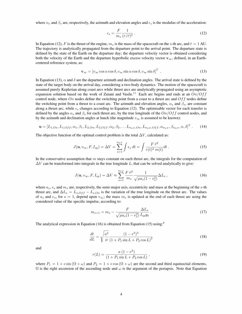
Results Figure 11 shows the curves ofBel and S corresponding to the 150 training points used to generatethe external surrogate models. Each curve represented in Figure 11 corresponds, therefore, to a differentvector of uncertain parameters, defined in the space Ξ, and to its corresponding feasible and optimal control.The figures also represent, by means of red vertical lines, the considered values of νmprop , ν∆r and ν∆v forProblems (36) and (37). The red horizontal lines represent the chosen values of 1−ε∆r, 1−ε∆v , 1−ε∆r,S and1− ε∆v,S . Feasible solutions to Problems (36) and (37) are given by the uncertain vectors and correspondingcontrols that, for the values of ν∆r and ν∆v identified by the red vertical lines, provide a Bel or S curve thatis above the red horizontal lines. Figures 12 show the Bel curves of the solutions of the iterative optimisationprocess described in Figure 4 to solve Problem 36. The maximum number of allowed iterations is 40. In orderto make the final results easier to visualise, Figures 13 show the Bel curves for the controls corresponding tothree uncertain vectors:

• the nominal uncertain vector ξnom (Table 2), represented in blue in Figure 13;

• the uncertain vector corresponding to the robust solution of Problem 36, identified by ξrob, and repre-sented in black in Figure 13;

• an additional solution found during the iterative process described in Figure 4, which does not satisfythe constraints defined in Problem 36. This solution is identified as ξnon−rob and it is shown in greenin Figure 13.

13

40 45 50 55

mprop

[kg]

40

45

50

55

(a) Accuracy of mprop.

0 0.5 1 1.5 2 2.5 3 3.5

r [km] 106

0

0.5

1

1.5

2

2.5

3

3.5106

(b) Accuracy of ∆r.

0 0.2 0.4 0.6 0.8 1

v [km/s]

0

0.2

0.4

0.6

0.8

1

(c) Accuracy of ∆v.

Figure 8: Relationship between mprop and mprop (a), ∆r and ∆r (b), and ∆v and ∆v (c).

Figure 13.a shows that the nominal solution has a Belief of the objective, for the chosen value of νmprop ,equal to 0.12. In order to get a Belief equal to 1 using the nominal control, the mass of propellant hasto be increased to 55.5 kg. The Belief of the constraints for the nominal solution are both equal to 1, forthe chosen values of ν∆r and ν∆v . The robust solution ξrob, identified solving Problem 36, has a valueof Bel(mprop ≤ νmprop) higher than the one of the nominal solution, equal to 0.74. Moreover, whenconsidering the robust solution, the Belief of the propellant mass reaches 1 when the mass of propellant isequal to 49 kg. The improvement in the Belief of the objective comes with a small reduction in the values ofBel(∆r ≤ ν∆r) and Bel(∆v ≤ ν∆v), which are, however, still above the chosen values of 0.95. Finally, thesolution ξnon−rob, represented in green, shows that the method presented in Figure 4 is capable of locatingmany different solutions, characterised by different values of the Belief for the objective and the constraints.The Belief of the propellant mass corresponding to ξnon−rob, which is equal to 1, is, in fact, higher than thecorresponding Belief of ξrob and ξnom. However, this comes with a reduction of Bel(∆v ≤ ν∆v) to a valuesmaller than 0.95.

During the iterations, the error due to the use of the external surrogate models is evaluated at each iteration,after the values of S for each ξopt are evaluated according to the method described in Figure 5. It is found

14

40

0.06

45

3.8

50

0.055 3.6

FL

0

[N]

55

v [km/s]

60

3.40.05 3.2

3

(a) Internal surrogate model mprop.

00.06

1

3.8

2

106

0.055 3.6

3

FL

0

[N] v [km/s]

4

3.40.05 3.2

3

(b) Internal surrogate model ∆r.

00.06

3.8

0.5

0.055 3.6

FL

0

[N] v [km/s]

1

3.40.05 3.2

3

(c) Internal surrogate model ∆v.

Figure 9: Example of internal surrogate models mprop (a), ∆r (b), and ∆v (c), for different values of FL0

and v∞ (x and y axis), and for fixed values of the other uncertain parameters.

that, during the 40 iterations, the errors are:

|S(mprop ≤ νmprop

)− S

(mprop ≤ νmprop

)| < 0.15

|S(

∆r ≤ ν∆r

)− S

(∆r ≤ ν∆r

)| < 0.03

|S(

∆v ≤ ν∆v

)− S

(∆v ≤ ν∆v

)| < 0.015

(38)

The errors are, therefore, limited to small values, and they are considered acceptable. It is important to stressthat the aim of the proposed method is to obtain a surrogate model that is locally accurate in the regionwhere the solutions of the considered problem are located; therefore, the surrogate models does not have tobe globally accurate in the entire design space. Figure 14 shows the control solution, in terms of azimuthand elevation angles during the transfer, for ξnom and ξrob. The difference in the control shown in Figure 14produces the difference in the Belief curves seen in Figure 13.

Computational Times In the following, the computational times required to complete each block in Fig-ures 4 and 5 are given. The computational times refer to a code run on Matlab R2017b on a machine withIntel(R) Core(TM) i7-3770 CPU @3.40 GHz and 8 GB RAM. In particular, with reference to Figure 5:

• The solution of the NLP problem takes ≈ 40 sec;

15

(a) External surrogate model Smprop .

(b) External surrogate model S∆r . (c) External surrogate model S∆v .

Figure 10: External surrogate model Sobj (a), S∆r (b), and S∆v (c).

• The creation of the internal surrogate models takes ≈ 40 sec;

• The computation of the Bel takes approximately 3 minutes, while the computation of the function Stakes 8 seconds. The difference in these computational times is due to the fact that the computation ofthe Belief requires a maximisation over each one of the 48 focal elements, for each one of the threefunctions mprop, ∆r and ∆v. The computation of the function S requires, instead, only the evaluationof these functions at a given number of points.

With reference to Figure 4:

• The computation time required for the computation of Bel and S, for all the N training points in Ξ,is given by the multiplication of N by the total computational time required to complete the diagramflow in Figure 5 (4 minutes and 30 seconds, approximately). In this case, N = 150 and the totalcomputational time to evaluate all the training points is, therefore, approximately 11.25 hours;

• The time required to create the external surrogate models for S, using the training points and DACE, is≈ 0.5 seconds;

• The time required to solve Problem (37), when 10000 function evaluations are considered for MP-AIDEA, is 10 seconds. As a comparison, if surrogate models of S were not used, and the complete

16

30 40 50 60 70

mprop

[kg]

0

0.2

0.4

0.6

0.8

1

Bel(m

pro

p<

mp

rop

)

(a) Bel(mprop ≤ νmprop

).

30 40 50 60 70

mprop

[kg]

0

0.2

0.4

0.6

0.8

1

S(m

pro

p<

mp

rop

)

(b) S(mprop ≤ νmprop

).

0 2 4 6 8 10 12

r [km] 106

0

0.2

0.4

0.6

0.8

1

Bel(

r <

r)

(c) Bel(

∆r ≤ ν∆r

)0 2 4 6 8 10 12

r [km] 106

0

0.2

0.4

0.6

0.8

1

S(

r <

r)

(d) S(

∆r ≤ ν∆r

)

0 0.5 1 1.5 2 2.5 3 3.5 4

v [km/s]

0

0.2

0.4

0.6

0.8

1

Bel(

v <

v

)

(e) Bel(

∆v ≤ ν∆v

)0 0.5 1 1.5 2 2.5 3 3.5 4

v [km/s]

0

0.2

0.4

0.6

0.8

1

S(

v <

v

)

(f) S(

∆v ≤ ν∆v

)Figure 11: Bel and S curves of the training points, corresponding to the objective (a and b), position

constraint (c and d), and velocity constraint (e and f).

process described in Figure 5 were to be realised, instead, at each function evaluation of the optimiser,the total computational time would have been 10000× 4.5 min ≈ 750 hours;

• The computation time to computeBel and S for ξopt is equal to the time required to complete the stepsin Figure 5, that is, approximately 4 minutes and 30 seconds;

• The time required to update the surrogate models for S is approximately 0.5 seconds.

17

30 40 50 60 70

mprop

[kg]

0

0.2

0.4

0.6

0.8

1

Be

l(m

pro

p<

mp

rop

)

(a) Bel(mprop ≤ νmprop

).

0 2 4 6 8 10 12

r [km] 106

0

0.2

0.4

0.6

0.8

1

Be

l( r

<

r)

(b) Bel(

∆r ≤ ν∆r

)0 0.5 1 1.5 2 2.5 3 3.5 4

v [km/s]

0

0.2

0.4

0.6

0.8

1

Be

l( v

<

v)

(c) Bel(

∆v ≤ ν∆v

)Figure 12: Bel and S curves of the results of the optimisation problem, corresponding to the objective (a),

position constraint (b), and velocity constraint (c).

CONCLUSION

This paper has presented the formulation and solution of the optimal control problem under uncertainty,where the uncertainty has been modelled using the Belief function of the Evidence Theory. In this work, thecomputation of the Belief function, which requires an optimisation over each focal element of the uncertaintyspace, has been sped up using internal surrogate models of the quantities to optimise. The original exactformulation of the problem, that uses the discontinuous Belief function, has then been transformed into aninexact formulation using a new continuous statistic function, S. The optimisation has then been realisedon the surrogate of the function S, rather than on the Belief. Moreover, by exploiting the correspondencebetween space of uncertainties and space of feasible and optimal controls, the optimisation has been realisedon the space of uncertainties, rather than on the higher dimensional space of the controls. The method hasbeen applied to the low-thrust transfer from Earth to asteroid Apophis. The considered uncertain parametersare the magnitude of the hyperbolic excess velocity at launch, and four parameters describing the thrust andspecific impulse of the low-thrust engine and their variation during the transfer.

The use of surrogate models and the optimisation on the uncertainty space, rather than on the space ofthe controls, have solved some of the challenge associated to the original formulation of the problem ofoptimisation under uncertainty, transforming the original problem into a manageable one, that can be solvedin a limited computational time. Moreover, results have shown that the proposed method is able to locate the

18

30 40 50 60 70

mprop

[kg]

0

0.2

0.4

0.6

0.8

1

Be

l(m

pro

p<

mp

rop

)

nom

rob

non-rob

55.5 kg

0.12

0.74

49 kg

1

(a) Bel(mprop ≤ νmprop

).

0 1 2 3 4 5 6 7 8

r [km] 106

0

0.2

0.4

0.6

0.8

1

Be

l( r

<

r)

nom

rob

non-rob

(b) Bel(

∆r ≤ ν∆r

)0 0.5 1 1.5 2

v [km/s]

0

0.2

0.4

0.6

0.8

1

Be

l( v

<

v)

nom

rob

non-rob

(c) Bel(

∆v ≤ ν∆v

)Figure 13: Belief of the nominal solution (ξnom), of the robust solution (ξrob), and of a non-robust solution(ξnon−rob).

control vector that provides a solution that is robust to uncertainties.

In this work, the proposed method has been applied to a problem with five uncertain parameters. Themethod could also be applied to higher dimensional problems. For higher dimensional problems, an increasedcomputational time has to be expected. The increase in computational time is due to the increase in thenumber of focal elements over which to realise the maximisation for the computation of the Belief of thetraining points of the external surrogate models. In addition, an increased number of training points wouldlikely be required to obtain sufficiently accurate initial external surrogate models.

Future work will be devoted to transform the constrained single-objective optimisation problem into amulti-objective optimisation problem, where the variables νmprop , ν∆r, ν∆v , ε∆r and ε∆v are also minimised.Moreover, the proposed method will be modified in order to extend the search for the robust solution to thespace of all the admissible controls, so as to include also the non-feasible and non-optimal controls.

ACKNOWLEDGEMENTS

This research has been developed with the partial support of the CNES grant R-S17/BS-0005-034 ”Ro-bust Optimization of Low-Thrust Interplanetary Trajectories” and the H2020 MCSA ITN UTOPIAE grantagreement number 722734.

19

0 100 200 300 400 500 600 700

L [deg]

-100

-50

0

[de

g] rob

nom

0 100 200 300 400 500 600 700

L [deg]

0

5

10

[deg

] rob

nom

Figure 14: Controls (azimuth and elevation angles α and β during the transfer) corresponding to ξnom andξrob.

REFERENCES

[1] M. Vasile, “Robust Mission Design Through Evidence Theory and Multiagent Collaborative Search,”Annals of the New York Academy of Sciences, Vol. 1065, 2005, pp. 152–173.

[2] N. Croisard, M. Vasile, S. Kemble, and G. Radice, “Preliminary space mission design under uncer-tainty,” Acta Astronautica, Vol. 66, 2010, pp. 654–664.

[3] G. Shafer, A Mathematical Theory of Evidence. Princeton University Press, 1976.[4] M. Vasile, E. Minisci, and Q. Wijnards, “Approximated Computation of Belief Functions for Robust De-

sign Optimization,” 53rd AIAA/ASME/ASCE/AHS/ASC Structures, Structural Dynamics and MaterialsConference, Honolulu, Hawaii, 2012, 2012.

[5] A. P. Dempster, “Upper and Lower Probabilities Induced by a Multivalued Mapping,” The Annals ofMathematical Statistics, Vol. 38, No. 2, April 1967, pp. 325–339.

[6] L. Zhang, “Representation, independence, and combination of evidence in the Dempster-Shafer theory,”Advances in the Dempster-Shafer theory of evidence (R. R. Yager, J. Kacpryk, and M. Fedrizzi, eds.),ch. 3, pp. 51–69, New York: John Wiley and Sons, 1994.

[7] K. Sentz and S. Ferson, “Combination of Evidence in Dempster-Shafer Theory,” tech. rep., SandiaNational Laboratories, 2002.

[8] M. Di Carlo, M. Vasile, and E. Minisci, “Multi-population inflationary differential evolution algorithmwith adaptive local restart,” 2015 IEEE Congress on Evolutionary Computation (CEC), 2015, pp. 632–639.

[9] F. Zuiani, M. Vasile, A. Palmas, and G. Avanzini, “Direct transcription of low-thrust trajectories withfinite trajectory elements,” Acta Astronautica, Vol. 72, 2012, pp. 108–120.

[10] M. Di Carlo, J. M. Romero Martin, and M. Vasile, “CAMELOT - Computational Analytical Multi-fidElity Low-thrust Optimisation Toolbox,” CEAS Space Journal, 2017.

[11] F. Zuiani and M. Vasile, “Extended analytical formulas for the perturbed Keplerian motion under aconstant control acceleration,” Celestial Mechanics and Dynamical Astronomy, Vol. 121, No. 3, 2015,pp. 275–300.

[12] S. N. Lophaven, H. B. Nielsen, and J. Sondergaard, “DACE - A Matlab Kriging Toolbox,” tech. rep.,Technical University of Denmark, 2002.

20