A Low-Frequency Instability/Oscillation near the …cfdku/papers/AIAA-2011-3548-448.pdfA Low-Frequency Instability/Oscillation near the ... 20th AIAA Computational Fluid Dynamics Conference

1 American Institute of Aeronautics and Astronautics

A Low-Frequency Instability/Oscillation near the Airfoil Leading-Edge at Low Reynolds Numbers and Moderate

Incidences

Ying Zhou1 and Z.J. Wang2 Department of Aerospace Engineering and CFD Center, Iowa State University, Ames, IA 50011

Numerical simulations of the low-Reynolds number ( ~ ) flows over a SD7003 airfoil at moderate incidences ( °) are performed in the current paper. A low-frequency convective instability is observed to dominate the spectrum near the leading edge and be responsible for the growth of the disturbance in the attached boundary layer. The characteristic frequency, the growth rate and the wave shape are investigated based on the numerical results. The growth of the low-frequency instability is not in agreement with parallel flow stability theory, nor with leading edge receptivity theory. And it has a higher growth rate than the Tollmien-Schlichting (T-S) wave. The effects of the angle-of-attack ( ), the Reynolds number and the airfoil geometry on the low-frequency instability are investigated and discussed.

NomenclatureAoA = angle of attack α = wave number of the disturbances in x direction in linear stability theory α = growth rate of the disturbances in linear stability theory β = wave number of the disturbances in z direction in linear stability theory c = chord length F, G, H = vector of fluxes i, j, k = index of coordinates in x, y, z direction J = Jacobian matrix M = Mach number p = nondimensional pressure Q, Q = vector of conservative variables in Cartesian coordiantes and standard unstructured elements Re = Reynolds number based on chord length ρ = nondimensional density s = wave speed of the disturbance in linear stability theory, s ω α⁄ St = Strouhal number, St fC sin AoA U⁄ in airfoil literature t = nondimensional time t t∗ c U⁄⁄ t∗ = dimensional time u, v, w = nondimensional velocity in x, y, z direction U = freestream velocity u′, v′, w′ = nondimensional velocity fluctuation in x, y, z direction u , u = nondimensional tangential velocity / fluctuation, normal to the wall surface x, y, z = nondimensional Cartesian coordinates ξ, η, ς = nondimensional coordinates in standard cubic ω = frequency of the disturbances ∆x , = cell size in wall units ∆y , ∆z Ω = computational spatial domain

1 Ph.D. Candidate, Dept. of Aerospace Engineering, 0245 Howe Hall, [email protected], AIAA student member. 2 Wilson Professor of Engineering, 2271 Howe Hall, [email protected], Associate Fellow of AIAA.

20th AIAA Computational Fluid Dynamics Conference27 - 30 June 2011, Honolulu, Hawaii

AIAA 2011-3548

Copyright © 2011 by Ying Zhou and Z. J. Wang. Published by the American Institute of Aeronautics and Astronautics, Inc., with permission.


I. Introduction N the past decade, low-Reynolds-number flows and the associated laminar separation bubbles (LSBs) have been of great interest in the development of micro air vehicles (MAV), small scale wind turbines and low-pressure

turbine/cascade. Since laminar boundary layers are less resistible to the significant adverse pressure gradient, LSBs are widely found over the suction side of low-Reynolds number airfoils/turbines at incidences. LSBs on an airfoil are classified into two types: a short bubble and a long bubble1. A short bubble is formed when the airfoil AoA is relatively small. The flow quickly transitions into a turbulent one and reattaches downstream after the breakdown of LSBs. A long bubble is formed at higher AoAs near the stall condition. For airfoils, the behavior of the LSB affects the aerodynamic performance and typically causes the increase of the pressure drag. Meanwhile, the existence of a turbulent boundary layer induces higher friction force on the airfoil than a laminar flow, and therefore can cause the degradation of the lift-to-drag ratio. Early works on LSB and associated hydrodynamic instability mechanisms can be traced back to the 1950s1 and 1960s2-5. With the rapid development of numerical methods, numerical simulations of laminar-separated flows have been used to investigate the LSB and the associated turbulent transition. The two-dimensional simulations of separation bubbles were first carried out and investigated by Pauley et al6. Pauley7 and Rist8 carried out three-dimensional studies of the primary instability later, but the transition was still not resolved due to the limitation of the computational resource and computer technology. More recently, direct numerical simulations (DNS) to fully resolve the transition of LSBs to turbulence were conducted by Alam & Sandham9 and also Spalart & Strelets10. With the development of experimental techniques, Laser-Doppler-Anemometry (LDA) and Particle-Image-Velocity (PIV) technologies can provide the flow field measurements to quantify the evolution of the unsteady flow structure and investigate the dynamics of LSBs (see Marxen et al.11; Lang et al.12; Hu & Yang13; Yarusevych et al.14; Hain et al.15). In spite of considerable progresses in recent years, both the LSB and the transition mechanism still need further investigation. Distinct from the convective types of transition, the simultaneous presence of and the interaction between separation and transition make the problem highly complicated.

In the present study, the numerical simulations of the low-Reynolds number flows over a SD7003 airfoil at incidences are carried out. A high-order spectral difference (SD) method for the three-dimensional Navier-Stokes equations on hexahedral grids developed by Sun et al. 16 is used. The simulations started with a uniform freestream initial condition and no incoming disturbances are added explicitly. The ‘short’ bubbles and transitional flows are observed on the suctions side of the airfoil under the present conditions. In previous studies of the unforced flow over airfoils, the LSBs and the self-sustained transition process were found owing to the global instability of the acoustic-feedback loops (see Deng et al.17; Zhou & Wang18; Jones et al.19). In the acoustic-feedback loop, the acoustic disturbances generated in the wake of the trailing edge act as the initial disturbances and the transition is triggered by the receptivity of the boundary layer to acoustic waves (Deng et al.17). Jones et al.19 found that the amplitude of the trailing-edge noise is sufficient to promote transition via the receptivity process in the vicinity of the leading edge and the feedback loop plays an important role in frequency selection of the vortex shedding that occurs in two dimensions.

The growth of the primary instability takes over a much longer distance comparing with the subsequent breakdown to turbulence. During the primary instability stage, the disturbances are amplified inside the attached boundary layer before separation and then inside the detached shear layer. After separation, an inflection point appears in the streamwise velocity profile. And the inviscid/Kelvin-Helmholtz (K-H) instability plays the dominant role in the growth of the disturbances. The inviscid flow has been found to be more unstable in a two-dimensional mode than in a three-dimensional mode according to the Rayleigh stability problem as shown in Drazin20. The two-dimensional disturbances grow exponentially inside the detached shear layer and the shedding of the two-dimensional vortices or ‘rolling’ is usually observed afterwards and the vortices grow in size after shedding. Yarusevych et al.21 investigated the behavior of the shedding vortices at different Reynolds numbers and angles of attack. It was found that the fundamental frequency of the roll-up vortices developing in the separated shear layer scales with the Reynolds number and the precise correlations depend on the angle of attack. In Hain et al. 15, a band of vortex shedding frequencies was found instead of a single frequency. Although the K-H instability is well accepted to be dominant after separation, the precursor of the K-H instability, which is responsible for the disturbance growth inside the attached boundary layer, is not clear yet. The well-known T-S instability is usually regarded as the dominant instability inside the attached boundary layer. Marxen et al.11 and Hein et al.15 conclude that transition was driven by convective amplification of a two-dimensional T-S wave. However, in Spalart & Strelets10, the T-S wave was discarded as the causes of the transition but a low frequency and long wavelength ‘wavering’ shear layer (or ‘flapping’) before separation was proposed because ‘the u′ profiles do not have the double-peak pattern of T-S waves’. Yang & Voke22 found in their study that the initial two-dimensional instability

I


waves grow downstream with an amplification rate usually larger than that of T-S waves. Watmuff23 suggested that that the shear layer is viscously stable with respect to small-magnitude T-S disturbances while it remains attached.

The current study focuses on the primary growth of disturbances on a low-Reynolds number airfoil at moderate incidences when ‘short’ bubbles occur, and a low-frequency instability is found to be dominant near the leading edge and responsible for the growth of disturbances. The growth of the low-frequency instability is not in agreement with the parallel flow stability theory, nor with the leading edge receptivity theory. The AoA, Reynolds number and the geometry of the airfoil are varied to investigate their effects on the frequency and the growth rate of the low-frequency instability. The paper is organized as follows. In § 2, a high-order method for unstructured hexahedral meshes used for the numerical simulation and a numerical method for the linear stability theory (LST) are introduced. After that, the computational details are given. In § 3, a low-frequency instability observed in the attached boundary layer near the leading edge is discussed. The effects of the AoA, the Reynolds number and the geometry of the airfoil on the low-frequency instability are studied. The computation results and associated details will be discussed in § 4, followed by the conclusions in § 5.

II. Numerical Methods

A. Review of Multidomain Spectral Difference (SD) Method We consider the unsteady three-dimensional compressible nonlinear Navier-Stokes equations written in the

conservative form as ∂Q∂t

∂F∂x

∂G∂y

∂H∂z

0 1

on domain Ω 0, T and Ω ⊂ R with the initial condition Q x, y, z, 0 Q x, y, z 2

and appropriate boundary conditions on ∂Ω.

Figure 1. Transformation from a physical element to a standard element

Figure 2. Distribution of solution points (circles) and flux points (squares) in a standard element for a 3rd-order SD scheme.


In SD method, it is assumed that the computational domain is divided into non-overlapping unstructured hexahedral cells or elements. In order to handle curved boundaries, both linear and quadratic isoparametric elements are employed, with linear elements used in the interior domain and quadratic elements used near high-order curved boundaries. In order to achieve an efficient implementation, all physical elements x, y, z are transformed into standard cubic element ξ, η, ς ∈ 1,1 1,1 1,1 as shown in Fig. 1.

In the standard element, two sets of points are defined (Fig. 2), namely the solution points and the flux points. The solution unknowns or degrees-of-freedom (DOFs) are the conserved variables at the solution points, while fluxes are computed at the flux points in order to update the solution unknowns. At the interfaces between each two elements, a Riemann solver such as Roe flux24 is used to compute the common inviscid flux, and the viscous flux at the interface is computed following the algorithm given in Ref. 25. A detailed description of the space discretization and the algorithm in SD method to compute the inviscid flux and viscous flux derivatives can be found in Ref. 16.

B. Review of the linear stability theory In this paper, the linear stability theory (LST) is used to analyze the stability characteristics of the attached

boundary layer and detached shear layer. The linear stability analysis of the velocity profiles are presented based on the time- and span-averaged flow field. Here, the flow is assumed compressible. The compressible LST used in this paper follows the procedure of Malik26. Under the assumptions of parallel flow and small disturbances, and neglecting high order terms, the linearized governing equations can be derived from the non-linear N-S equations (1). By assuming the disturbances of the following travelling waves

ϕ ϕ e , 3 where α and β are the complex wavenumber in the x and z directions respectively, and ω is the complex frequency of the travelling wave. Substituting (3) into the linearized governing equation, we obtain the following system of ordinary differential equations

Addy

Bddy

C ϕ 0, 4

where ϕ u, v, p, T, w and matrices A, B and C can be found in Malik26. The boundary conditions for equation (4) are

y 0;u v w 0; 0 (adiabatic wall)

y ∞;u, v, T, w → 0.0 Equation (4) constitutes an eigenvalue problem, which can be solved to find the complex dispersion relation

ω ω α, β for the temporal mode, or α α ω, β for the spatial mode: 1) Aϕ ωBϕ for temporal stability 2) Aϕ αBϕ for spatial stability where ω or α is the eigenvalue and ϕ is the discrete representation of the eigenvector.

For spatial stability, the eigenvalue is determined by the determinant condition Det|A αB| 0 5

Equation (5) represents the dispersion relation of α α ω, β , and in this paper we employ the single domain spectral (SDSP) collocation method to discretize equation (5). The eigenvalue problem of the discretized equation can be solved with Linear Algebra PACKage (LAPACK) or Matlab software. The current code was verified through comparison with the LST results of viscous supersonic plane Couette flow in Hu & Zhong27.

C. Details of numerical simulations The numerical simulations are carried out at a Reynolds number based on the airfoil chord of Re 6 10 and

Mach number M 0.2 . The AoA of the baseline case is AoA 4° . All the variables in this paper are non-dimensional unless noted. Figure 3 shows the computational mesh for the current simulation. The mesh is refined near the wall and around the physically important region where the separation bubble and vortex breakdown occur. The smallest cell is located at the trailing edge with dimension (in wall units) ∆y 2.5 in the direction normal to the wall, ∆x 25.0 along the chord and ∆z 12.0 in the spanwise direction. Noting that inside the cell each direction is discretized by the solution/flux points (Fig. 2), the effective grid size near the wall for 3rd and 4th-order SD method is close to the requirement of a direct numerical simulation (DNS). The total number of cells is 253,600, resulting in 6,847,200 and 16,230,400 degree-of-freedom (per equation) for the 3rd and 4th-order SD schemes respectively. The grid resolution has been verified in previously published papers28 and good agreements of the mean and statistical results were found in a p-type grid refinement study.


In order to simulate an infinite wing, a periodic boundary condition is used in the spanwise direction. The span width of the wing is set to be 20% of the chord, which has been proved to be adequate long enough in Ref. 28. A non-slip, adiabatic boundary condition is applied on the surface of the wing. Near the far-field of the computational domain, the absorbing sponge zone (ASZ) 29 is used to absorb the out-going disturbances.

Figure 3. Computational mesh.

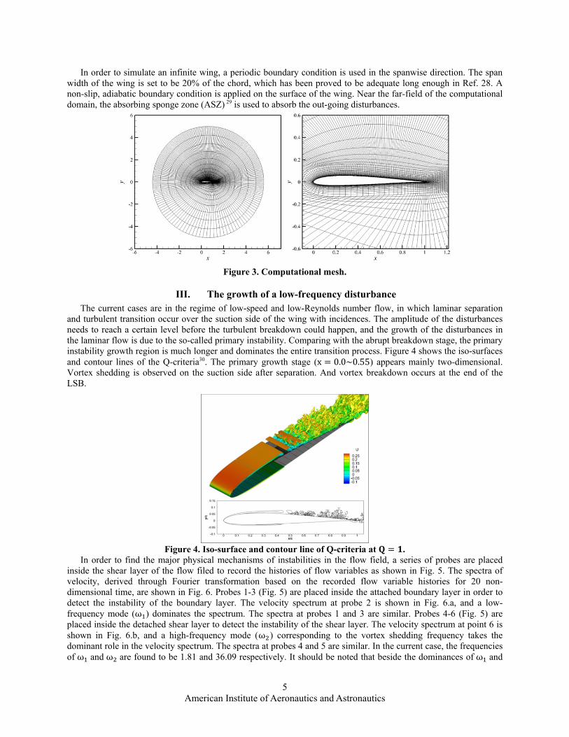
III. The growth of a low-frequency disturbance The current cases are in the regime of low-speed and low-Reynolds number flow, in which laminar separation

and turbulent transition occur over the suction side of the wing with incidences. The amplitude of the disturbances needs to reach a certain level before the turbulent breakdown could happen, and the growth of the disturbances in the laminar flow is due to the so-called primary instability. Comparing with the abrupt breakdown stage, the primary instability growth region is much longer and dominates the entire transition process. Figure 4 shows the iso-surfaces and contour lines of the Q-criteria30. The primary growth stage (x 0.0~0.55) appears mainly two-dimensional. Vortex shedding is observed on the suction side after separation. And vortex breakdown occurs at the end of the LSB.

Figure 4. Iso-surface and contour line of Q-criteria at .

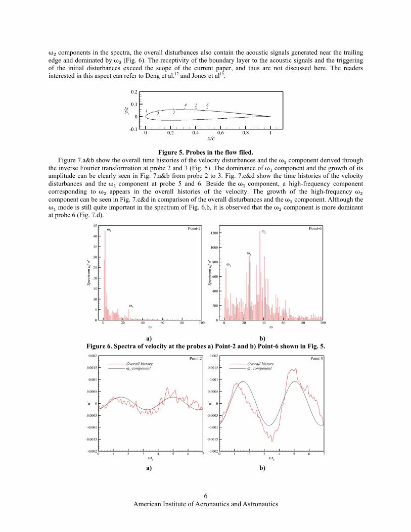
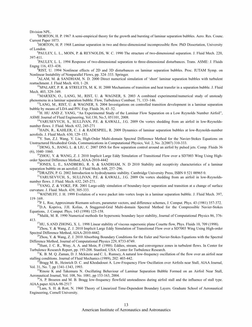
In order to find the major physical mechanisms of instabilities in the flow field, a series of probes are placed inside the shear layer of the flow filed to record the histories of flow variables as shown in Fig. 5. The spectra of velocity, derived through Fourier transformation based on the recorded flow variable histories for 20 non-dimensional time, are shown in Fig. 6. Probes 1-3 (Fig. 5) are placed inside the attached boundary layer in order to detect the instability of the boundary layer. The velocity spectrum at probe 2 is shown in Fig. 6.a, and a low-frequency mode (ω ) dominates the spectrum. The spectra at probes 1 and 3 are similar. Probes 4-6 (Fig. 5) are placed inside the detached shear layer to detect the instability of the shear layer. The velocity spectrum at point 6 is shown in Fig. 6.b, and a high-frequency mode (ω ) corresponding to the vortex shedding frequency takes the dominant role in the velocity spectrum. The spectra at probes 4 and 5 are similar. In the current case, the frequencies of ω and ω are found to be 1.81 and 36.09 respectively. It should be noted that beside the dominances of ω and


ω components in the spectra, the overall disturbances also contain the acoustic signals generated near the trailing edge and dominated by ω (Fig. 6). The receptivity of the boundary layer to the acoustic signals and the triggering of the initial disturbances exceed the scope of the current paper, and thus are not discussed here. The readers interested in this aspect can refer to Deng et al.17 and Jones et al19.

Figure 5. Probes in the flow filed. Figure 7.a&b show the overall time histories of the velocity disturbances and the ω component derived through

the inverse Fourier transformation at probe 2 and 3 (Fig. 5). The dominance of ω component and the growth of its amplitude can be clearly seen in Fig. 7.a&b from probe 2 to 3. Fig. 7.c&d show the time histories of the velocity disturbances and the ω component at probe 5 and 6. Beside the ω component, a high-frequency component corresponding to ω appears in the overall histories of the velocity. The growth of the high-frequency ω component can be seen in Fig. 7.c&d in comparison of the overall disturbances and the ω component. Although the ω mode is still quite important in the spectrum of Fig. 6.b, it is observed that the ω component is more dominant at probe 6 (Fig. 7.d).

a) b) Figure 6. Spectra of velocity at the probes a) Point-2 and b) Point-6 shown in Fig. 5.

a) b)


c) d)

Figure 7. Time histories of the velocity disturbances and the component derived through the inverse Fourier transformation at probe points (Fig. 5): a) Point-2; b) Point-3; c) Point-5; d) Point-6.

Both the ω and ω components are convectively unstable as shown in Fig. 7. And it seems that the ω component leads the growth of the overall disturbances in the attached boundary layer, while the ω component dominates in the detached shear layer. Figure 8.a shows the normalized profiles of the mean tangential velocity at different locations and Fig. 8.b shows the corresponding normalized profiles of RMS tangential velocity disturbances at the corresponding locations. The mean flow separates at x 0.225 and the development of the mean shear layer and the detachment can be seen in Fig. 8.a. The profiles of the RMS of tangential velocity disturbance u change the shapes along the mean shear layer as shown in Fig. 8.b. It appears that due to the dominances of the ω and ω components at different locations, the shape of the disturbance profile has two difference patterns in the attached boundary layer and the detached shear layer. In the following, the two types of the profile are further investigated. In order the detect the characters of the instabilities, the LST is applied based on the mean flow field and the LST results are used for comparison with the numerical results.

a) b)

Figure 8. Numerical results for Case-4: a) normalized profiles of the mean tangential velocity at different locations; b) normalized profiles of the RMS tangential velocity disturbances at different locations.

a) b) Figure 9. Comparison of the RMS of the tangent velocity disturbances and the LST results at a) . and b) . .


Inside the attached boundary layer, a T-S wave is usually thought to be the dominant instability which causes the growth of the disturbances. However, in the present cases, the T-S wave does not appear to play a role here. Based on the mean profile at x 0.1, the most unstable T-S wave predicted by the LST appears at a frequency ω119.85, which is much higher than the dominant frequency ω 1.81. The profile of the RMS of u in the current numerical simulation is presented in Fig. 9.a, and the profiles of the most unstable T-S wave at ω 119.85 and the T-S wave corresponding to ω 1.81 are also shown for comparison. It is observed that the RMS of u does not possess the two-peak feature of the normal T-S waves. Spalart and Strelets10 found a good agreement between the peak location of the RMS of u profile and the peak location of du dn⁄ (n being the wall normal direction) profile. Table 1 compares the wave speed and growth rate of the numerical and LST results. The wave speed and the growth rate of the numerical simulation are derived based on the numerical results, which can be seen in detail in the next section. It can be seen that at frequency ω 1.81, the T-S wave is predicted to be stable. Meanwhile the growth rate of the low-frequency instability is much higher than that of the predicted most unstable T-S wave (also see Yang & Voke22).

After separation, an inflection point is observed in the mean velocity profiles shown in Fig. 8.a and the K-H instability becomes more dominant. Figure 9.b shows the profiles of the disturbances at x 0.55. The LES curve denotes the profile of the overall disturbances, and the LST curve is the profile of the most unstable (has the highest growth rate) K-H mode. Although the curve of the numerical simulation contains all the modes, the LST curve predicts the peaks and valleys of the profile quite well, as at x 0.55 the vortex shedding frequency dominates the spectrum. Table 2 compares the wave speed and growth rate of the present numerical simulation and LST results and the agreement is quite good for this stage. The most unstable wave found in the LST based on the mean profiles at x 0.55 has been found to be ω 39.85, which is quite close to the frequency ω 36.09 of the shedding vortices. Meanwhile, the growth rate of the most unstable wave ω predicted with LST is α 29.10 and is also in very good agreement with the growth rate of the shedding vortices α 30.17 as shown in Table 2.

The T-S wave component is not visible in the attached boundary layer near the leading edge. The K-H instability in the present cases is similar to but not a purely inviscid instability due to the viscous effects near the wall. From the LST, it is found that the K-H instability in the present cases belongs to the family of the T-S instability. In comparison with the LST results, the low-frequency instability seems not of the T-S wave type and appears to be an unusual mechanism to the authors, while the high-frequency instability agrees well with the LST results. For better understanding of the low-frequency instability, the AoA, Reynolds number and the airfoil geometry are varied to study the associated characters in the following sections.

Table 1. Comparison between LES and LST results at . ω s α

LES 1.81 0.53 16.69LST 119.85 0.63 3.30LST 1.81 0.18 stable

Table 2. Comparison between LES and LST results at .

Frequency ω Wavespeeds α LES 36.09 0.55 30.17 LST 39.85 0.56 29.10

A. Angle-of-attack effects In this section, the numerical simulations are carried out at AoA 2° and 6° for comparison with the baseline

case and the AoA effects on the low-frequency instability are investigated based on the numerical results at all three AoAs. In the following text, each case is named after its AoA at which it has been carried out, i.e. Case-2 represents the case at AoA 2° and so on so forth. In order to quantitatively study the growth of the disturbances, probes are placed at the locations of the velocity RMS peaks as shown in Fig. 10.a-c to record the histories of flow variables in the primary growth region of all three cases. The RMSs of u recorded with the probes along the streamwise direction are shown in Fig. 10.d-f. Note that the shape of the growth curves is quite similar in all three cases. According to the rate of disturbance growth α, the overall growth of the disturbances can be divided into two major stages by a sign change of d α dx⁄ and the region between the two stages is the transient region. dα dx⁄ , the changing of the growth rate measures the tendency of the instability and the sign change of d α dx⁄ indicates the extremum of the tendency.

As discussed above that the two frequencies ω and ω are found to be dominant in the attached and detached shear layers respectively, it is natural to find that the two major growth stages are caused by the two types of


instabilities respectively. The dash line in Fig. 10.e derived through the inverse Fourier transformation based on the recorded variable histories shows the contribution of disturbance growth from the ω component for Case-4. Note that the overall growth of disturbances is dominated by the low frequency component (ω ) for a long distance from x 0.0 to x 0.5. The dash-dot line in Fig. 10.e shows the contribution of the disturbance growth from the K-H instability ω for Case-4. After x 0.5 the ω component decays and the ω component grows from a very small amplitude ~10 after the separation point x 0.225. It can be seen in Fig. 10.e that the K-H instability leads to the second major growth of the overall disturbances in Case-4, and similar processes can be observed in the other two cases (Fig. 10.d and Fig. 10.e). The growth trend of the overall disturbances in Case-4 agrees well with the spectra shown in Fig. 6 and the evolvement of the disturbance RMS profile shown in Fig. 7.b.

The average growth rates of the instabilities in the two stages are labeled in Fig.s 10.d-f for all three cases. The growth rate of the low-frequency ω instability is high near the leading edge and gradually decreases in the streamwise direction. And the average growth rate of the low-frequency instability increases with the AoA. Table 3 lists the frequencies of ω and ω for all three cases, and the frequency ω decreases with the AoA. The Strouhal number lies around St 0.02 as shown in Table 3. It is interesting to find that the Strouhal number St 0.02 is close to that of the low-frequency oscillation of the LSB on airfoils near stall condition in the literatures31-34. Near stall condition the ‘long’ LSBs were found to oscillate at a very low frequency, and the Strouhal numbers of the low-frequency are reported to be ranging from St 0.005~0.02 in Ref. 31-34, which is much lower than that of the oscillating wake of a bluff body (St 0.2). Here, it seems the low-frequency oscillation also exists in current ‘short’ bubbles.

Table 3. Characteristic frequencies and Strouhal number

Case AoA ω St ω Case‐2 2° 3.42 0.019 22.22Case‐4 4° 1.81 0.020 36.09Case‐6 6° 1.09 0.018 60.73

a) b) c)

d) e) f) Figures 10. Numerical results of Case-2, Case-4 and Case-6 (left to right): a-c): location of probes in the flow filed; d-f): RMS tangential velocity disturbances at locations of probes.

B. Effects of Reynolds number It has been seen previously that the low-frequency instability and the K-H instability are two-dimensional. For

saving the computation time and being efficient, two-dimensional simulations are carried out in this section to investigate the Reynolds number effects on the low-frequency instability. Four cases in Reynolds number range Re 3 10 ~1.2 10 at AoA 4° are performed by changing the viscosity as listed in Table 5. The baseline case at Re 6 10 is also included here. The contour line of Q-criteria of the instantaneous flow field and the spanwise vorticity contour of the mean flow field are shown in Fig. 11 for all cases. With the increase of the


Reynolds number, the scale of the shedding vortices and the region of the separated flow decrease (Fig. 11). The separation is almost avoided at Re 1.2 10 . The low-frequency component is again observed to be dominant in the attached boundary layer of all cases.

Table 5 lists the frequency, the corresponding Strouhal number and the mean growth rate of the ω component for all the cases. Like the T-S and K-H instability, the frequency and growth rate can be largely affected by the Reynolds number. The frequency of ω decreases with the increase of the Reynolds number, which results in the Strouhal number in a range of St 0.005~0.130. Although the Strouhal number at Re 3 10 is close to that of the oscillating wake of a bluff body, the rest Strouhal numbers locates in a similar range in which the near stall low-frequency oscillation was observed. The average growth rate of the ω component does not have a monotone trend with the increase of the Reynolds number. And the baseline case has the highest growth rate among all the four cases.

a)

b)

c)

d)

Figure 11. The contour line of Q-criteria of the instantaneous flow field (left) and the spanwise vorticity contour of the mean flow field (right). a) Case-Re-1; b) Case-Re-2; c) Case-Re-3; d) Case-Re-4.

Table 5. Characteristic frequency, Strouhal number and growth rate

Case Re ω St α Case‐Re‐1 3 10 11.365 0.1262 1.672Case‐Re‐2 6 10 3.565 0.0396 18.230Case‐Re‐3 9 10 3.450 0.0383 13.438Case‐Re‐4 1.2 10 0.401 0.0045 11.920

C. Effects of airfoil geometry The effects of airfoil geometry on the low-frequency instability are further tested in this section. By changing the

camber length of the original SD7003 airfoil, two cases are carried out at the same condition as the baseline case at Re 6 10 , Ma 0.2 and AoA 4°. As listed in Table 6, the airfoil geometries in Case-G-1 and Case-G-2 are


derived by decreasing and increasing the baseline camber length by 25% respectively. Again, two dimensional simulations are carried out for computation time saving and efficiency. The 2D baseline model Case-Re-2 is also included for comparison.

Table 6 lists the frequency, the corresponding Strouhal number and the mean growth rate of the ω component for the three cases. Both the frequency and growth rate vary monotonically with the camber length. The low-frequency ω increases with the increase of the camber length, and the Strouhal number varies slightly around 0.038.

Table 6. Characteristic frequency, Strouhal number and growth rate Case ω St α

Case‐G‐1 3.311 0.0368 9.436Case‐Re‐2 3.565 0.0396 18.230Case‐G‐2 3.723 0.0413 22.334

a)

b)

Figure 12. The contour line of Q-criteria of the instantaneous flow field (left) and the spanwise vorticity contour of the mean flow field (right). a) Case-G-1; b) Case-G-2.

IV. Discussions The present paper documents data on a phenomenon of two-dimensional low-frequency instability/oscillation of

flow over an airfoil that is different in many ways from the well-known T-S wave. The instability wave oscillates at a much lower frequency but has a much higher growth rate than the T-S wave. It was suggested by Jones et al.19 that during the process of receptivity the Lam-Rott eigensolutions (Lam & Rott35) of the linearized boundary layer equation is excited near the leading edge and the wavelength is much larger than that of a T-S wave. The Lam-Rott disturbance which is caused by non-parallel flow effects was found to be excited in the boundary layer receptivity process. It decreases in both amplitude and wavelength in the streamwise direction, and finally continues as a T-S wave (also see Goldstein36 and Ricco & Wu37). In addition, the leading effect of a non-zero pressure gradient is to introduce a purely oscillatory factor into the disturbances as discussed in Lam & Rott35. However, a similar process is not observed here in all three cases. Unlike the Lam-Rott eigensolutions, the low-frequency wave is unstable and the decreasing of its wavelength in streamwise direction to continue as a T-S wave is not observed in all present cases. The K-H disturbances grow from a small amplitude ~10 instead of being excited by the low-frequency disturbances. Near the leading edge with the increase of the AoA, the pressure gradient and growth rate of the low-frequency instability increase, but the frequency of the low-frequency decreases. However, since the airfoil flow is very complicated and usually nonlinear, the changes of the frequency and growth rate at different AoA are unlikely to be purely caused by the change of the pressure gradient. Although the pressure gradient effects are still not clear, the low-frequency instability seems unlikely to be the Lam-Rott disturbance suggested by Jones et al19.

Flapping of the laminar separated bubble (LSB) was observed in many previously published works of low-Reynolds number flows10,38,39. The flapping is an up-and-down motion of the separated shear layer. However, the low-frequency instability/oscillation dominant in the attached boundary layer does not appear to be caused directly by the downstream flapping of the LSB to the authors. Figure 12 shows histories of the ω velocity component in the range of x 0.1~0.25 for the two dimensional baseline case Case-Re-2, which are derived using the inverse Fourier transformation based on the recorded velocity histories. It could be seen clearly through the peaks and valleys that the wave is downstream convective and unstable, rather than caused by the wavering of the shear layer


associated with the flapping of the downstream LSB. The same conclusion can also be derived by comparing Fig. 7.a and Fig. 7.b. Spalart and Strelets10 suggested that the transition mechanism involves the wavering/flapping of the shear layer and then K-H vortices. A wavering shear layer was defined to have a dependence of the type u x, y, z, t u x, y y , where y x, z, t is a statistical variable with small variations. The formula represents that the wave oscillates in y direction (normal direction). However, at the current Reynolds numbers the transverse viscosity wave is unlikely to sustain and thus their hypothesis of the wavering behavior of the shear layer seems inappropriate. The up-and-down flapping motion of the separated shear layer seems more likely to be combination result of the low-frequency oscillation in the attached boundary layer upstream and the pressure change inside the bubble.

Figure 12. The histories of the velocity component in the range of . ~ . in Case-Re-2.

V. Conclusions Various questions have remained unanswered but the following inferences have been clearly made: (1) A low-

frequency oscillation in the attached boundary layer is observed in the present study. The low-frequency instability is found to be apparently two dimensional and convective unstable. (2) The primary growth of the disturbances before the turbulent breakdown over the suction side of the airfoil consists of two stages. The first stage is dominated by the low-frequency instability and the second growth stage is caused by the K-H instability. (3) The phenomenon is hydrodynamic in nature. The low-frequency instability is neither the famous T-S instability nor the result of the Lam-Rott eigensolutions of the receptivity theory. And it seems not to be caused by the flapping of the downstream bubble and the detached shear layer.

The low-frequency oscillation in the present cases occurs in the Strouhal number range of St 0.005~0.130, and the Strouhal numbers are in the same magnitude of the low-frequency oscillation of the airfoil flow near stalling conditions as reported in several previously published papers. It is conjectured that the low-frequency instability in the present cases may be the same mechanism of the near stall low-frequency oscillation. It is interesting to find that the Strouhal number keeps almost constant at moderate AoA 2°, 4° and 6°. In the testing of the airfoil geometry effects, the frequency and growth rate vary monotonically with the camber length. However, unlike the low-frequency oscillation near the stalling condition, the Strouhal number and the growth rate of the low-frequency instability change largely with the Reynolds number.

Acknowledgments

The authors would like to acknowledge the support from the Air Force Office of Scientific Research and the Department of Aerospace Engineering, Iowa State University.

References 1Owen, P. R. and Klanfer, L. On the laminar boundary layer separation from the leading edge of a thin aerofoil. 1953 ARC

Conf. Proc. 220. 2GASTER, M. 1963 On stability of parallel flows and the behaviour of separation bubbles. PhD Dissertation, University of

London. 3GASTER, M. 1967 The structure and behaviour of separation bubbles. Aero. Res. Counc. R&M 3595. Aerodynamics


Division NPL. 4HORTON, H. P. 1967 A semi-empirical theory for the growth and bursting of laminar separation bubbles. Aero. Res. Counc.

Current Paper 1073. 5HORTON, H. P. 1968 Laminar separation in two and three-dimensional incompressible flow. PhD Dissertation, University

of London. 6PAULEY, L. L., MOIN, P. & REYNOLDS, W. C. 1990 The structure of two-dimensional separation. J. Fluid Mech. 220,

397-411. 7PAULEY, L. L. 1994 Response of two-dimensional separation to three-dimensional disturbances. Trans. ASME: J. Fluids

Engng 116, 433–438. 8RIST, U. 1994 Nonlinear effects of 2D and 3D disturbances on laminar separation bubbles. Proc. IUTAM Symp. on

Nonlinear Instability of Nonparallel Flows, pp. 324–333. Springer. 9ALAM, M. & SANDHAM, N. D. 2000 Direct numerical simulation of ‘short’ laminar separation bubbles with turbulent

reattachment. J. Fluid Mech. 410, 1–28. 10SPALART, P. R. & STRELETS, M. K. H. 2000 Mechanisms of transition and heat transfer in a separation bubble. J. Fluid

Mech. 403, 329–349. 11MARXEN, O., LANG, M., RIST, U. & WAGNER, S. 2003 A combined experimental/numerical study of unsteady

phenomena in a laminar separation bubble. Flow, Turbulence Combust. 71, 133–146. 12LANG, M., RIST, U. & WAGNER, S. 2004 Investigations on controlled transition development in a laminar separation

bubble by means of LDA and PIV. Exp. Fluids 36, 43–52. 13H. HU AND Z. YANG, “An Experimental Study of the Laminar Flow Separation on a Low Reynolds Number Airfoil”,

ASME Journal of Fluid Engineering, Vol.130, No.5, 051101, 2008. 14YARUSEVYCH, S., SULLIVAN, P.E. & KAWALL, J.G. 2009 On vortex shedding from an airfoil in low-Reynolds-

number flows. J. Fluid. Mech. 632, 245-271 15HAIN, R., KAHLER, C. J. & RADESPIEL, R. 2009 Dynamics of laminar separation bubbles at low-Reynolds-number

aerofoils. J. Fluid Mech. 630, 129–153. 16Y. Sun, Z.J. Wang, Y. Liu, High-Order Multi-domain Spectral Difference Method for the Navier-Stokes Equations on

Unstructured Hexahedral Grids, Communications in Computational Physics, Vol. 2, No. 2(2007) 310-333. 17DENG, S., JIANG, L. & LIU, C. 2007 DNS for flow separation control around an airfoil by pulsed jets. Comp. Fluids 36

(6), 1040–1060. 18ZHOU, Y. & WANG, Z. J. 2010 Implicit Large Eddy Simulation of Transitional Flow over a SD7003 Wing Using High-

order Spectral Difference Method, AIAA-2010-4442 19JONES, L. E., SANDBERG, R. S. & SANDHAM, N. D 2010 Stability and receptivity characteristics of a laminar

separation bubble on an aerofoil. J. Fluid Mech. 648, 257–296. 20DRAZIN, P. G. 2002 Introduction to hydrodynamic stability. Cambridge University Press, ISBN 0 521 00965 0. 21YARUSEVYCH, S., SULLIVAN, P.E. & KAWALL, J.G. 2009 On vortex shedding from an airfoil in low-Reynolds-

number flows. J. Fluid. Mech. 632, 245-271. 22YANG, Z. & VOKE, P.R. 2001 Large-eddy simulation of boundary-layer separation and transition at a change of surface

curvature. J. Fluid. Mech. 439, 305-333. 23WATMUFF, J. H. 1999 Evolution of a wave packet into vortex loops in a laminar separation bubble. J. Fluid Mech. 397,

119–169. 24P. L. Roe, Approximate Riemann solvers, parameter vectors, and difference schemes, J. Comput. Phys. 43 (1981) 357-372. 25D.A. Kopriva, J.H. Kolias, A Staggered-Grid Multi-domain Spectral Method for the Compressible Navier-Stokes

Equations, J. Comput. Phys. 143 (1998) 125-158. 26Malik, M. R. 1990 Numerical methods for hypersonic boundary layer stability, Journal of Computational Physics 86, 376-

413. 27HU, S.AND ZHONG, X. L. 1998 Linear stability of viscous supersonic plane Couette flow, Phys. Fluids 10, 709 (1998). 28Zhou, Y. & Wang, Z. J. 2010 Implicit Large Eddy Simulation of Transitional Flow over a SD7003 Wing Using High-order

Spectral Difference Method, AIAA-2010-4442. 29Zhou, Y. & Wang, Z. J. 2010 Absorbing Boundary Conditions for the Euler and Navier-Stokes Equations with the Spectral

Difference Method, Journal of Computational Physics 229, 8733-8749. 30Hunt, J. C. R., Wray, A. A. and Moin, P. (1988). Eddies, stream, and convergence zones in turbulent flows. In Center for

Turbulence Research Report, pp. 193-208. Stanford, USA: Center for Turbulence Research. 31K. B. M. Q. Zaman, D. J. Mckinzie and C. L. Rumsey, A natural low-frequency oscillation of the flow over an airfoil near

stalling conditions. Journal of Fluid Mechanics (1989), 202: 403-442. 32Bragg M. B., Heinrich D. C. and Khodadoust A. Low-Frequency Flow Oscillation over Airfoils near Stall, AIAA Journal,

Vol. 31, No. 7, pp 1341-1343, 1993. 33Rinoie K and Takemura N. Oscillating Behaviour of Laminar Separation Bubble Formed on an Airfoil Near Stall,

Aeronautical Journal, Vol. 108, No. 1081, pp 153-163, 2004. 34A. P. Broeren and M. B. Bragg low-frequency flowfield unsteadiness during airfoil stall and the influence of stall type.

AIAA paper AIAA-98-2517 35Lam, S. H. & Rott, N. 1960 Theory of Linearized Time-Dependent Boundary Layers. Graduate School of Aeronautical

Engineering, Cornell University.


36GOLDSTEIN, M. E. 1983 The evolution of Tollmien–Schlichting waves near a leading edge. J. Fluid Mech. 127, 59–81. 37P. RICCO AND X. WU. Response of a compressible laminar boundary layer to free-stream vortical disturbances. J. Fluid

Mech., 587:97–138, 2007. 38Wissink, J. & Rodi, W. 2004 DNS of a Laminar Separation Bubble Affected by Free-Stream Disturbances.

Springer/Kluwer Academic. 39Wilson, P. G. & Pauley, L. L. 1998 Two- and three-dimensional large-eddy simulations of a transitional separation bubble.

Phys. Fluids 10, 2932–2940.

Documents

A Low-Frequency Instability/Oscillation near the …cfdku/papers/AIAA-2011-3548-448.pdfA Low-Frequency Instability/Oscillation near the ... 20th AIAA Computational Fluid Dynamics Conference