Copyright ©1997, American Institute of Aeronautics and Astronautics, Inc.

AIAA Meeting Papers on Disc, January 1997A9715768, F49620-94-1-0019, F49620-95-1-0405, AIAA Paper 97-0756

Direct numerical simulation of hypersonic boundary-layer transition over bluntleading edges. II - Receptivity to sound

Xiaolin ZhongCalifornia Univ., Los Angeles

AIAA, Aerospace Sciences Meeting & Exhibit, 35th, Reno, NV, Jan. 6-9, 1997

This paper presents results of the direct numerical simulation (DNS) of the generation of boundary layer instability wavesdue to freestream acoustic disturbances, for a 2D Mach 15 flow over a parabola. The full Navier-Stokes equations are solvedby using a new explicit fifth-order shock-fitting upwind scheme for both steady and unsteady flow solutions. The DNSresults are also compared with local linear stability analysis based on mean flow solutions obtained by the numericalsimulation. The numerical results show that the instability waves developed in the hypersonic boundary layer behind the bowshock contain both the first- and second-mode instabilities. The results also indicate that external disturbances, especially theentropy and vorticity ones, enter the boundary layer to generate instability waves mainly in the leading-edge region. (Author)

Page 1

Direct Numerical Simulation of Hypersonic Boundary-Layer Transition OverBlunt Leading Edges, Part II: Receptivity to Sound

Xiaolin Zhong *University of California, Los Angeles, California 90095

Abstract

The receptivity of a hypersonic boundary layer tofreestream disturbances, which is the process of envi-ronmental disturbances initially entering the boundarylayer and generating the growth of instabilities, is al-tered considerably by the presence of the bow shockin the flow field. This paper presents results of thedirect numerical simulation (DNS) of the generationof boundary layer instability waves due to freestreamacoustic disturbances, for a two-dimensional Mach 15flow over a parabola. The full Navier-Stokes equationsare solved by using a new explicit fifth-order shock-fitting upwind scheme (AIAA 97-0755) for both steadyand unsteady flow solutions. The DNS results are alsocompared with local linear stability analysis based onmean flow solutions obtained by the numerical simula-tion. The numerical results show that the instabilitywaves developed in the hypersonic boundary layer be-hind the bow shock contain both the first and secondmode instabilities. The results also indicate that exter-nal disturbances, especially the entropy and vorticityones, enter the boundary layer to generate instabilitywaves mainly in the leading edge region.

Introduction

The prediction of laminar-turbulent transition in hy-personic boundary layers is a critical part of the aero-dynamic design and control of advanced hypersonicvehicles f1'^. In general, the transition is a result ofnonlinear response of the laminar boundary layers toforcing disturbances '3~6-'. The forcing disturbances ^can originate from many difference sources, includ-ing freestream disturbances. In an environment withsmall initial disturbances, the paths to transition con-sist of three stages: 1) receptivity, 2) linear eigenmodegrowth or transient growth, and 3) nonlinear break-down to turbulence. The first stage is the receptiv-ity process ™\ which converts the environmental dis-turbances into instability, Tollmien-Schlichting (T-S),

'Assistant Professor, Mechanical and Aerospace EngineeringDepartment, xiaolin@seas.ucla.edu, Member AIAA.

Copyright ©1997 by American Institute of Aeronautics and As-tronautics, Inc. All rights reserved.

waves in the boundary layers. The second stage isthe linear eigenmode growth of boundary-layer insta-bility waves obtained as the eigen-solutions of the ho-mogeneous linearized disturbance equations. The rele-vant instability waves developed in hypersonic bound-ary layers are the T-S wave and inviscid waves of higher(Mack) modes discovered by Mack '9'10J, the Gortlerinstability'11-' over concave surfaces, and the three-dimensional cross flow instability '12l The third stageis the breakdown of linear instability waves and transi-tion to turbulence after the growth of linear instabilitywaves reach certain magnitudes.

The receptivity mechanism provides important ini-tial conditions of amplitude, frequency, and phase forthe instability waves in the boundary layers t13"15!.The theoretical results on incompressible boundarylayer receptivity are mainly based on the asymp-totic theory'16'17'. The asymptotic analysis explainshow the long wavelength freestream acoustic distur-bances enter the boundary layer and generate short-wavelength T-S waves in incompressible boundary lay-ers. The direct numerical simulation, which solvesthe full Navier-Stokes equations as an initial-boundaryproblem by numerical methods, has recently becomean important tool in receptivity and transition studies.The DNS of the receptivity of incompressible bound-ary layers has been performed by Murdock '-18''; Lin,Reed, and Saric[19]; Buter and Reed [20]; Casalis andCantaloube[21]; and Collis and Lele [22].

For hypersonic flow over blunt bodies, the receptiv-ity phenomena are much more complex and are cur-rently still poorly understood I23'24'. Figure 1 showsa schematic of wave field interactions near the hyper-sonic leading edge affected by freestream disturbances.Kovasznay '25-' showed that weak disturbance waves incompressible flow can be decomposed into three inde-pendent modes: acoustic, entropy, and vorticity modes.The acoustic wave is propagated with the speed ofsound relative to the moving fluid, while the entropyand vorticity waves convect with the moving fluid ve-locity. Before entering the boundary layer, freestreamdisturbances will be first processed by the bow shock.Irrespective of the nature of the freestream disturbancewave, its interaction with the bow shock always gen-erates all three types of disturbance waves '26'. These

transmitted disturbance waves are propagated down-stream and interact with the boundary layer on thebody. At the same time, the boundary layer will alsogenerate reflected acoustic wave impinging on the shockfrom behind and generating further disturbances to theshock and wave fields. All these interactions will affectthe transition of the hypersonic boundary layer behindthe shock.

Many theoretical and experimental studies have doneon hypersonic boundary layer transition. Reshotko andKhan ̂ showed that the swallowing of the entropylayer, which is created by the curved bow shock, bythe boundary layers has strong effects on the stabil-ity of the boundary layers. The experimental mea-surements on hypersonic boundary layer stability onsharp cones showed the additional complexity of hy-personic boundary layers I28"30!. The results indicatedthat the first and second mode instabilities are simul-taneously present in the hypersonic boundary layers.Experiments on hypersonic boundary layer transitionover blunt cones I31~33J show that slight nose bluntnesshas significant effects on the boundary layer transition.The increase of nose bluntness delays the transition on-set, but the trend is reversed when the nose bluntnessexceeds a certain limit. In addition, Stetson et al. '33-'found evidence of inviscid entropy instability in the re-gion outside of the boundary layers for the case of cer-tain blunt cones at Mach 8 freestream in the entropy-layer swallowing region.

The stability characteristics of hypersonic bound-ary layers over a blunt cone corresponding to Stetson'sexperiments ^^ have been studied using the linear sta-bility theory (LST) by Malik et al.[34], Herbert andEsfahanian ias\ and Kufner et al. t36>375. Though someobservations on the effects of bluntness and the entropylayer are consistent with linear stability analysis, thesecond-mode instability and the general amplificationcharacteristics in the blunt cone flows do not agree withthe experiments. The discrepancy may be due to thefact that the LST of hypersonic flow over a blunt conehas the difficulty of obtaining highly-accurate steadybase flow for the stability equations. The results ofLST are very sensitive to the accuracy of the baseflows. In addition, the effects of the bow shock andnon-parallel boundary layers on the disturbances fieldsare not considered in the LST. The receptivity phe-nomena, which become very complex due to hypersonicbow shock interaction t23>24J; are also neglected in thelinear stability analysis. The discrepancy between theLST and experiments may be resolved by the DNS ifthe neglected physical effects in LST are properly ac-counted for in the DNS.

The purpose of our research is to study the receptiv-

ity of hypersonic boundary layers behind blunt bod-ies by direct numerical simulation and compare theDNS results with LST ones. We ̂ started our re-search efforts by investigating the inviscid interactionbetween the bow shock and freestream disturbances intwo-dimensional hypersonic flow past a cylinder. Theresults show that with the body effects, there is awide range of wavelengths for the entropy and vorticitywaves behind the shock and their wavelengths reduceto zero at the wall. On the other hand, the wavelengthsof the acoustic waves do not change very much in thepresence of the body. The numerical results also showthat the pressure, density, and vorticity perturbationsare amplified considerably by the back and forth reflec-tion of disturbance waves between the shock and thebody. Such interaction and reflection also increase themagnitude of bow-shock oscillation.

In this paper and a companion paper ^39\ we ex-tend the previous inviscid studies to the direct numer-ical simulation of the receptivity of hypersonic bound-ary layers to free stream acoustic waves. The di-rect numerical simulation approach studies the tran-sitional boundary layers '-40' by numerically solving thetime-dependent three-dimensional Navier-Stokes equa-tions for the temporally or spatially evolving instabilitywaves. Such simulation requires that all relevant flowtime and length scales are resolved by the numerical so-lutions using highly accurate numerical methods. Oneof the difficulties in hypersonic flow DNS is that high-order schemes are required for the direct simulations,however, high-order linear schemes can only be used forthe spatial discretization of the equations in the flowfields without shock waves.

In Ref. [39], we presented a new high-order (fifthand sixth order) upwind finite difference shock fittingmethod for the direct simulation of hypersonic flowwith a strong bow shock and with stiff source terms.There are three main aspects of the new method forhypersonic flow DNS: a new shock fitting formula-tion, new upwind high-order finite difference schemes,and third-order semi-implicit Runge-Kutta schemes re-cently derived t41'. The review of other current DNSworks, the details of the new method, and the resultsof evaluation of numerical accuracy of the new schemescan be found in Ref. [39].

The purpose of this paper is to investigate the re-ceptivity of hypersonic flows to free stream acousticwaves by DNS using the new fifth-order upwind explicitshock fitting method presented in Ref. [39]. In gen-eral, three dimensional unsteady flow should be consid-ered in the DNS studies since the most unstable firstmode in hypersonic boundary layers are oblique three-dimensional instability waves ™, though the most un-

stable second mode is two dimensional. In this pa-per, only the two-dimensional instability waves in hy-personic boundary layers are considered as a first stepof the DNS of three-dimensional hypersonic boundarylayers over blunt bodies. The free stream disturbancesare planar acoustic waves with a fixed frequency, andthe body is a parabolic leading edge. The generationof T-S waves in the boundary layer are studied basedon the DNS results. The numerical accuracy of theDNS results for such hypersonic boundary layer recep-tivity have been evaluated by grid refinement studiesand have been reported in Ref. [39]. These test resultsare not presented here.

Governing Equations

The governing equations for the direct numericalsimulations of hypersonic flows over a blunt wedge arethe unsteady three-dimensional Navier-Stokes equa-tions in the following standard conservation-law form:

where the viscous stresses are given by

where p.* is the viscousity coefficient, The viscosity co-efficient is calculated using the Sutherland's law,

/T*•jf = n* I £_

r'r I m*V-'O

3/2 ,

T*+T*

and A* = -2//*/3. The heat flux vectors are

_ _9j ~

(8)

(9)

where K* is the heat conductivity coefficient computedby assuming a constant Prandtl number Pr.

OU*dt* dxj (1)

where superscript "*" represents dimensional variables,and

U" = {p", P*ul, p"ul, p"ul, e*} (2)

(3)

The gas is assumed to be thermally and colorically per-fect gas,

(4)

where the gas constant R* and the specific heats C£and C* are assumed to be constants with a given ratioof specific heats 7. The flux vectors are

(5)

77* _f Vj —

k *?*«*•

(6)

Nondimensionalization of Variables

We nondimensionalize the velocities with respect tothe freestream velocity U^, length scales with respectto a reference length d*, density with respect to p"^,pressure with respect to p^, temperature with respectto T£Q, time with respect to d* /U^, vorticity with re-spect to U^/d*, entropy with respect to C*, wave num-ber by 1/d*, etc. The dimensionless flow variables aredenoted by the same dimensional notation but withoutthe superscript "*".

Problem Description and Flow Conditions

The receptivity of a two-dimensional boundary layerto weak freestream acoustic disturbance waves for aMach 15 hypersonic flow past a parabolic leading edgeat zero angle of attack are considered. The wave fieldof the unsteady viscous flows are represented by theperturbations of instantaneous flow variables with re-spect to their local mean variables. For example, theinstantaneous velocity perturbation u' is defined as theperturbations with respect to local mean velocity, i.e.,

u' = u'(x,y,t) - u(x,y,t) - U(x,y) (10)

where U(x,y) is the dimensionless mean flow velocity.

In the simulation, the freestream disturbances are su-perimposed on the steady mean flow to investigate the

development of T-S waves in the boundary layer withthe effects of the bow shock interaction. The freestreamdisturbances are assumed to be weak monochromaticplanar acoustic waves with wave front normal to thecenter line of the body. The perturbations of flow vari-able introduced by the freestream acoustic wave beforereaching the bow shock can be written in the followingform:

P'P1

\v'\\P'\\P'\

where \u'\, \u'\, \p'\, and \p'\ are perturbation ampli-tudes satisfying the following relations:

Kloo = Hoo = 0

\P\oo =

where e is a small number representing the freestreamwave magnitude. The parameter k is the dimension-less freestream wave number which is related to thedimensionless circular frequency u by:

(12)

The corresponding dimensionless frequency F is de-nned as

(13)

The body surface is a parabola given by

x* =b*y*2-d* (14)

where b* a given constant and d* is taken as the ref-erence length. The body surface is assumed to be anon-slip wall with an isothermal wall temperature T£.

The specific flow conditions are:

Moo = 15

2£, = 192.989 KT* = 1000 KR* - 286.94 Nm/kgKb* = 40 m'1rr* = 288 KH* = 0.17894 x IQ-^ksNose Radius of Curvature = r* = 0.0125mRe<* = P*^U*d*/n* - 6026.55

e = 5 x 10-4

p^ = 10.3 Pa7= 1.4Pr = 0.72d* = 0.1m17 = 110.33 #

Numerical Methods and Grids

The receptivity problems are studied by numericallysolving the unsteady nonlinear Navier-Stokes equationsusing our new fifth-order shock fitting scheme t39'. Thetest results of the new shock fitting schemes and thenumerical accuracy of calculating the receptivity prob-lems of hypersonic viscous flows are presented in Ref.[39], and they are not presented here.

The numerical simulation for an unsteady hypersoniclayer receptivity problem is carried out in three steps.First, a steady flow field is computed by advancing theunsteady flow solutions to convergence using the fifth-order computer code. No disturbances are imposed inthe freestream. The steady shock shape is obtained asa part of the numerical solutions. Second, unsteadyviscous flows are computed by imposing a continu-ous planar acoustic single-frequency disturbance waveon the steady flow variables at the freestream side ofthe bow shock according Eq. (11). The subsequentshock/disturbance interactions and generation of T-Swaves in the boundary layer are solved without lin-earization using the full Rankine-Hugoniot relations atthe shock and the Navier-Stokes equations in the flowfields. The unsteady calculations are carried about for10 to 20 periods in time until the solutions reach aperiodic state. Third, the unsteady computations arecarried out for one additional period in time to performFFT on the perturbation field to obtain the Fourier am-plitude and phase of the perturbations of the unsteadyflow variables throughout the flow field.

In the calculations, smooth unsteady body fittedgrids are used to treat the unsteady bow shock mo-tion as an outer computational boundary. Figure 2shows a schematic of the general 3-D shock fitted gridsused in the simulation. The grids are stretched in bothstreamwise and the wall-normal directions. The gridstretching function along the wall-normal grid lines (£= constant) are

R(n,t) = H(t,t) (15)

(0 < T) < 1)

where R(JJ) is distance from the body surface to a gridpoint along a wall normal grid line, and ft is a smallnumber chosen to be 1.01. H(£,t), which is an un-known solved along with the flow variables, is the nor-mal distance between the shock and the body surfacealong the same grid line. The stretching function for

grid points along the body surface is

S($=S (a (16)

where S(£) is the curve length along the body surface,S is the total curve length, and a\ is a constant chosento be 0.45 in the calculations. The unsteady bow shockshape and movement are solved as part of the compu-tation solutions. Analytical formulas for the metriccoefficients for coordinates transformation are used toensure numerical accuracy for the unsteady coordinatetransformation in the simulations. More details can befound in Ref. [39].

Steady Flow Solutions

The steady flow solutions of the Navier-Stokes equa-tions for the viscous hypersonic flow over the parabolaare obtained by using the new fifth-order explicit un-steady computer code and advancing the solutions to asteady state without freestream perturbations. It hasbeen found that the accuracy of the stability analysisfor hypersonic boundary layers is very sensitive to theaccuracy of the mean flow solutions ̂ . By using thenew high-order shock-fitting scheme, we are able to ob-tain high-accuracy "clean" mean flow solutions for theunsteady calculations as well as for the LST analysesfor the same hypersonic boundary layer.

Figure 3 shows steady flow solutions for a set of160 x 120 computational grid, velocity vectors, andsteady entropy contours. Since the bow shock shape isobtained as the solution for the freestream grid line, theconvergence of the steady state solutions can be mea-sured by the solutions for the bow shock velocity. Thenormal velocity solutions of the bow shock should reachzero when the solutions reach a true steady states. Forthe numerical solutions shown in Fig. 3, the numericalsolutions for the dimensionless bow shock normal ve-locities are 2 x 10~13 and 5 x 10~10 for two shock pointslocated at the center line and at the exit boundary re-spectively. Therefore, these solutions are consideredto be at steady state and are used as the mean flowsolutions for the unsteady flow simulation.

The velocity vector plot in Fig. 3 also shows the de-velopment of the boundary layer along the surface. Theentropy contours show the entropy layer developing atthe edge of the boundary layer. The swallowing of theentropy layer by the boundary layer has been shown toplay an important role in the stability and transition ofthe boundary layer downstream '•27\ The figure showsthat the entropy layer begins to enter the outer regionof the boundary layer when x > 1.

Figure 4 shows the variation of steady flow pres-sure, temperature, and tangential and normal veloci-ties along a range of wall-normal grid lines at several igrid stations. The i index of the grid lines plotted inthe figures are between 50 and 100. The x coordinatesof the intersecting points of grid lines and the surface

Table 1. x coordinates for surface grid points.Index i5060708090100110120130140150

xs Coordinates-0.756873-0.663535-0.557069-0.435716-0.297524-0.1404390.03765050.2388920.4654540.7195151.00326

The pressure plot in Fig. 4 and the steady pressure dis-tribution along the body surface shown in Fig. 5 showthat the flow has a favorable pressure gradient alongthe body surface. Figure 4 also shows that the flowdistribution across the boundary layer for the presenttest case is very different from a hypersonic boundarylayer over a flat plate. Specifically, the velocity andother flow variables do not reach a constant asymp-totic states outside the boundary layer, and the normalvelocity components un are about 10% of the tangen-tial velocity ut due to curvature effects. Therefore, itis expected that the stability properties will be differ-ent from those of obtained from LST analysis which isbased on parallel base flow assumptions.

For compressible flat plate boundary layers, Lin andLees '42J showed that there is a generalized inflectionpoint for inviscid instability which corresponds to thezeros of d(pdu/dyn)/dy. Stetson et al. I33' found evi-dence of inviscid entropy instability in the region out-side of the boundary layers for the case of certain bluntcones at Mach 8 freestream in the entropy-layer swal-lowing region. Figure 6 shows the variation of baseflow entropy and p(dut/dyn) along grid lines normal toparabola surface at several i grid stations. The lowerfigures show that when i < 80 (x = 0.44 on surface),there is only one generalized inflection point neat thewall, as i increases, an additional zero of the derivativeof d(pdut/dyn)/dyn appears at the outer region of theboundary layers. At the same time, the main gener-alized inflection point move further and further awayfrom the wall as i increases. This may explain the de-velopment of second mode structure in the boundary

layer in that region for the unsteady results presentedbelow.

Unsteady Flow Solutions

In this section, the generation of boundary-layer T-S and inviscid instability waves by freestream acousticdisturbances is considered for hypersonic flow over aparabolic leading edge with various freestream distur-bance wave numbers or frequencies. The dimensionlessfreestream wave numbers are chosen to be k = 15,12.5,and 10, and the corresponding dimensionless frequencyF x 10~6 are 2655, 2212, 1770, respectively. The fre-quencies used in the simulation are higher than thoseused in other DNS studies of the receptivity of incom-pressible boundary layers *19'. The current F valuesare chosen mainly as an initial test cases. We will ex-tend our studies to lower frequency regimes in futurestudies.

Unless stated explicitly, we will mainly present theresults for the case of wave number k = 15 with thefreestream disturbance parameter e = 5 x 10~4.

Mode Structure of Instability Waves

Figure 7 shows the contours for the instantaneousperturbation v' of the velocity in y direction after theflow field reach a periodic state, the Fourier amplitude\v'\ and the phase angle <pv (in degrees). The unsteadycomputations are run for more than 27 periods in timeto ensure that periodic solutions have been reached forthe entire flow field.

The instantaneous contours of v' show the develop-ment of instability waves in the boundary layer on thesurface. In general, the disturbances field v' is a com-bination of the external forcing disturbance waves andthe T-S waves in the boundary layer. For receptiv-ity problems of incompressible boundary layers, thecomponents of the T-S waves are decomposed '20' fromthe forcing disturbances by recognizing the fact thatthe freestream wave lengths are an order of magni-tude longer than those of the T-S waves in the bound-ary layers. For hypersonic boundary layers, however,such decompositions are not possible because the wavelength of the forcing disturbances and the instabilitywaves in the boundary layers are of the same orderof magnitudes. In addition, the external disturbancewaves are very complex due to the back and forth re-flection and interaction of the waves. Though we cannot separate the external waves from the T-S wave inthe boundary layer, Figure 7 shows very clearly thedevelopment of instability waves in the boundary layeralong the surface. The reason is because the insta-

bility waves are dominant in the boundary layer nearthe surface. Meanwhile the waves immediately behindthe bow shock are mainly external forcing waves. Thefigure also show that the wave lengths are very closefor the instability waves in the boundary layer and theexternal waves at the shock.

From the instantaneous contours in Fig. 7, it is clearthat the instability waves developed in the wall havetwo separate zones. The first zone is located in theregion of x < 0.2 and the second one is located in theregion of a; > 0.2. The peak oscillations for the wavein the first region are very close to the wall surface andthere is mainly one peak in the oscillation magnitudesacross the boundary layer. The second region developsoscillations away from the wall with two magnitudepeaks. These results suggest that the instability wavedeveloped in the first region of x < 0.2 is the first modeinstability and that in the second region of x > 0.2 isdominated by the second mode instability wave.

The contours of the Fourer amplitudes and phase an-gles for v' in Fig. 7 also show the switching of instabilitymodes from region 1 to region 2 at about x = 0.2 on thesurface. The decay of first mode and the growth of thesecond mode is shown by a sudden phase change nearthe body surface around a; = 0.2. The phase structurehas one more variation across the boundary layer afterthe change of modes.

The wave field development along the body surfaceis shown by the variation of entropy perturbation s'along the the surface. Figure 8 shows the distribu-tion of instantaneous entropy perturbations along theparabola surface. The distribution of the Fourier am-plitudes and phase angles of the entropy perturbationsalong the parabola surface are shown in Figs. 9 and10 respectively. These figures show the distinct twomain region of instability waves. In the phase angleplots of Fig. 10, there is a sudden change of phase an-gle near x = 0.2. Fig. 9 also show that the first modeis much stronger than the second mode for the testcase at this particular frequency. The first and secondmodes are more clearly shown by the distribution ofthe local growth rates based on peak entropy pertur-bations along the parabola surface as shown in Fig. 11.The growth rate is defined as

-a, = dS (17)

where S is the surface curve length. Though the sec-ond mode has much higher local growth rates, its am-plitudes are lower than those of the first mode becausethe second mode is confined to a narrower region.

The variation of amplitudes of pressure perturba-tions along grid lines normal to parabola surface atseveral * grid stations is shown in Fig. 12. The cor-responding variations for tangential velocity perturba-tions are shown in Fig. 13. The corresponding x co-ordinates for the grid points on surface are given byTable 1. The first three stations (a)-(c) of i are lo-cated in region of first mode instability,, station (d)is located at the mode switching region, and the lasttwo stations (e) and (f) are located in the second modeinstability region. The figure shows that the ampli-tude structure is very different between the two modes.Mack t10! defines the first and second mode in flat plateboundary layer by the structure of the real part of theeigenfunctions of the pressure perturbations. Figure14, which is taken from Ref. [10], shows the pressure-fluctuation eigenfuction (real part) of first six modesof 2D inflectional neutral waves for flat plate boundarylayer at Mach number 10. The number of zeros in theeigenfunctions was used by Mack to identify the modenumbers for compressible boundary layers. Figure 15shows the variation of the real part of Fourier trans-form for the pressure perturbations obtained by thenumerical simulations for the present case. The modestructure inside the boundary layer shows that it is thefirst mode in the first zone and the second mode in thesecond zone.

Comparison with Local Parallel Linear Analysis

Though the mean flow for the present flow betweenthe bow shock and the parabola is not parallel, a linearstability analysis based on parallel mean flow assump-tion is carried out using the steady mean flow obtainedby the current numerical simulation. Since the en tran-sition prediction method based on LST is the primarytool in boundary-layer transition prediction, the pur-pose for the comparison is to investigate how the DNSand LST will differ in hypersonic boundary layers withbow shocks.

The LST code is a temporal code developed by Huand Zhong '43' based on both a fourth-order finite dif-ference global method and a spectral global method.The results from the two methods are compared toensure numerical resolution for the instability modes.The code has been tested for compressible Couette flowand compressible boundary layer calculations by com-paring its results with published results and with DNSresults '39J. The Gaster's transformation '44' is used toconvert the temporal stability results into spatial sta-bility results.

The preliminary calculations on linear stability ofthe hypersonic flows over the parabola at grid sta-tions i = 70 and i = 100 have been carried out. The

dimensionless frequencies (nondimensionalized by d*)predicted by the LST are compared with that used inthe DNS:

Table 2. LST and DNS results on FI Xs

70 -0.557069100 -0.140439

F ID'6 (LST)1912.71715.0

F ID-" (DNS)1769.951769.95

The results agree reasonably well considering the factthat LST is based on a parallel flow assumption. Figure16 shows the distribution of the local growth rate alongthe parabola surface for LST and DNS results. The fig-ure shows LST results under-predict the growth rate atstation i = 70, but they over-predict the growth rate aat station i = 100. The disagreement on growth ratebetween LST and experimental results are well known,and no satisfactory explanation has been reached ^s\The DNS results provide much more detailed informa-tion of the instability fields. We are currently inves-tigating the cause of the disagreement in the growthrates with the help of DNS results. Possible causes in-clude the effects of the bow shock, the effects of strongnon-parallel mean flows, etc.

Generation of Instability Waves by Incident Waves

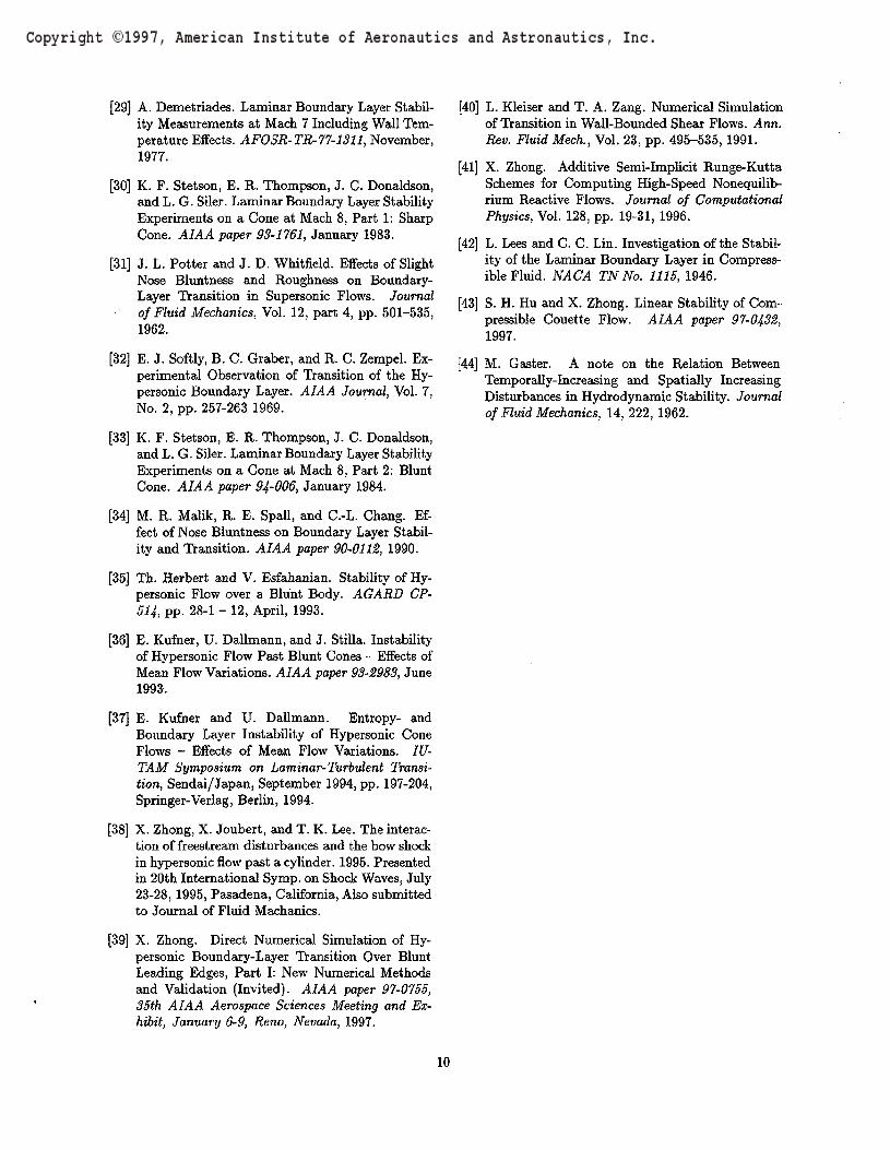
For incompressible boundary layers, it has been re-ported in experimental and theoretical analysis thatthe external waves enter the boundary mainly in theleading edge regions. For hypersonic flows over ablunt body, any freestream waves interaction with theshock always generate a combination of all three kindsof waves: acoustic (pressure), entropy, and vorticitywaves. In an effort to isolate the effects of these threewaves, the instantaneous contours of pressure, entropy,and vorticity perturbations of flow variables are plot-ted in Fig. 17. The entropy and vorticity contours showvery clearly that the external waves enter the bound-ary and generate T-S waves in the boundary mainly inthe leading edge region of x < —0.7 for the present testcase. Figure 18 shows a local instantaneous contoursat the leading edge region for entropy perturbations.

In a previous paper, Zhong et al. '38J show that theinviscid entropy and vorticity waves based on the Eu-ler equations are singular at the stagnation point. Sucha singularity creates a wide range of length scales forthese waves near the leading edge region. Though thesingularity is removed in the viscous flow solutions, theentropy and vorticity waves have strong interaction athe leading edge regions. The figure also shows thatthere is very little interaction between the external en-tropy and vorticity waves and the T-S waves in theboundary layers.

On the other hands, the pressure contours in Pig. 17shows that the acoustic disturbances interact with theT-S waves in the boundary both in the leading edgeregion and downstream region.

Effects of Frequency

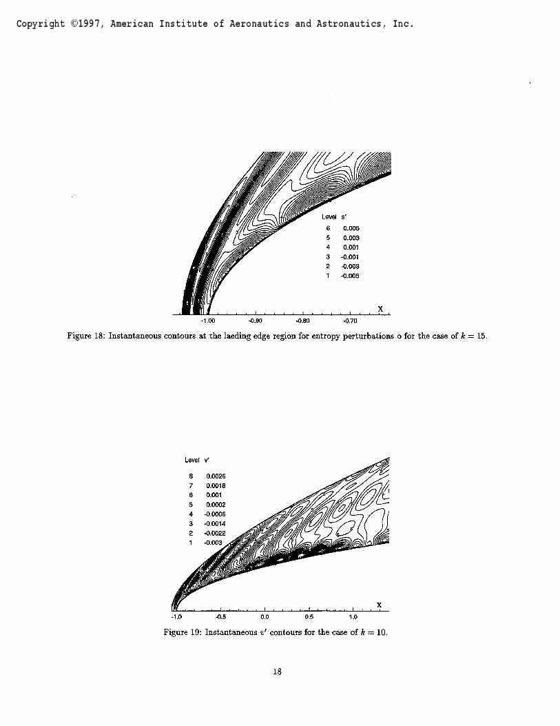
Several test cases with different freestream frequencyF (or freestream waves number k) are used to investi-gate the effects of frequency on the T-S waves in theboundary layer. Figure 20 shows the distribution ofthe amplitudes of the entropy perturbations along theparabola surface for three cases of different freestreamwave numbers. The figure shows that the first modeinstability region becomes longer as the frequency de-creases, and the second mode instability region appearsat further downstream with higher local Reynold num-bers. The overall growth of the disturbance amplitudesare much higher as the frequency decreases. The in-stantaneous v' contours for the case of lower wave num-ber at k = 10 shows that the first mode instability re-gion extends to much longer range and is much strongerin amplitude. Figure 21 shows the distribution of thelocal growth rates along the parabola surface for threecases of different freestream wave numbers. Again, thefigure shows that the length of the first-mode instabil-ity region increases as frequency decreases.

Shock Oscillations

In the unsteady simulations, the bow shock oscil-lates due to freestream disturbances and the reflec-tion of acoustic waves from the boundary layer to theshock. It is important that the numerical simulationresolves the unsteady shock motion accurately. Thecurrent high-order shock fitting method is found to beable to compute the unsteady flow fields and the un-steady shock motion very accurately. A simple wayto check the accuracy of the numerically computedunsteady shock/disturbances interaction is shown inFig. 22, which shows the time history of the instanta-neous pressure perturbation at the point immediatelybehind the bow shock at the center line for the caseof k = 40. In the initial moment of imposing thefreestream disturbances, there is no reflected wavesfrom the undisturbed steady boundary layer. Thefreestream disturbance wave transmission relation canbe predicted by linear theory such as that derived byMckenzie and Westphal ^26l At later time, the wavepattern changes because the disturbance waves enterthe boundary layer and generate reflected waves backto the shock. The figure shows very good agreementbetween DNS and linear predictions on the pressureperturbation due to freestream disturbances.

Figure 23 shows the numerical results of the instan-

taneous normal bow shock velocities vs. the shock xcoordinates for the case of k = 15. Notice that thereis no different mode of unsteady motion at the shock,which is outside of boundary layer.

Conclusions

The receptivity of a hypersonic boundary layerto freestream monochromatic planar acoustic distur-bances has been studied by direct numerical simula-tions (DNS) for a two-dimensional Mach 15 flow over aparabola. The full Navier-Stokes equations are solvedby using a new explicit fifth-order shock-fitting upwindscheme. The DNS results are also compared with locallinear stability analysis based on mean flow solutionsobtained by the numerical simulation. The numericalresults show the following conclusions:

1. The instability waves developed in the hypersonicboundary layer behind the bow shock contain boththe first and second mode instabilities. The sizeand the strength of the two regions depend on thefrequency of the disturbances.

2. The results indicate that external disturbances,especially the entropy and vorticity ones, enterthe boundary layer to generate instability wavesmainly in the leading edge region.

3. LST results compare reasonably well with DNSresults on frequency, but the agreement is not asgood on the growth rates. These results are con-sistent with the comparisons between LST and ex-perimental results for hypersonic boundary layersover axisymmetric cones.

Acknowledgments

This research was supported by the Air Force Of-fice of Scientific Research under grant numbers F49620-94-1-0019 and F49620-95-1-0405 monitored by Dr. LenSakell. The author would like to thank Mr. S. Hu forproviding LST results for comparison and Mr. T. Leefor providing results for shock/disturbances analyticalresults.

References

[1] National Research Council (U.S.). Committee onHypersonic Technology for Military Application.Hypersonic Technology for Military Application.Technical Report, National Academy Press, Wash-ington, DC., 1989.

[2] Defense Science Board. Final Report of the Sec-ond Defense Science Board Task Force on the Na-tional Aero-Space Plane (NASP). AD-A274530,94-00052, November, 1992.

[3] Th. Herbert and M. V. Morkovin. Dialogue onBridging Some Gaps in Stability and TransitionResearch. In Laminar-Turbulent Transition, IV-TAM Symposium, Stuttgart, Germany, 1979, R.Eppler, H. Fasel, Editors, pp. 47-72, Springer-Verlag Berlin, 1980.

[4] M. V. Morkovin and E. Reshotko. Dialogue onProgress and Issues in Stability and Transition Re-search. In Laminar-Turbulent Transition, IUTAMSymposium, Toulouse, France, 1989, D. Arnal, R.Michel, Editors, Springer-Verlag Berlin, 1990.

[5] E. Reshotko. Boundary Layer Instability, Transi-tion and Control. AIAA paper 94-0001, 1996.

[6] Th. Herbert. Progress in Applied Transition Anal-ysis. AIAA paper 96-1993, 27th AIAA Fluid Dy-namics Conference, New Orleans, LA, June, 1996.

[7] D. Bushnell. Notes on Initial Disturbance Fieldfor the Transition Problem. Instability and Tran-sition, Vol. I, M. Y. Hussaini and R. G. Viogt,editors, pp. 217-232, Springer-Verlag, 1990.

[8] M. Morkovin. On the Many Faces of Transi-tion. Viscous Drag Reduction, C.S. Wells, editor,Plenum, 1969.

[9] L. M. Mack. Linear Stability Theory and theProblem of Supersonic Boundary-Layer Transi-tion. AIAA Journal, Vol. 13, No. 3, pp. 278-289,1975.

[10] L. M. Mack. Boundary layer linear stability the-ory. In AGARD report, No. 709, 1984.

[11] W. S. Saric. Gotler Vortices. Annual Review ofFluid Mechanics, Vol. 26, pp. 379-409, 1994.

[12] H. L. Reed and W. S. Saric. Stability of Three-Dimensional Boundary Layers. Annual Review ofFluid Mechanics, Vol. 21, pp. 235-284, 1989.

[13] M. Nishioka and M. V. Morkovin. Boundary-LayerReceptivity to Unsteady Pressure Gradients: Ex-periments and Overview. Journal of Fluid Me-chanics, Vol. 171, pp. 219-261 1986.

[14] M. E. Goldstein and L. S. Hultgren. Boundary-Layer Receptivity to Long-Wave Free-Stream Dis-turbances. Annual Review of Fluid Mechanics,Vol. 21, pp. 137-166 1989.

[15] Saric W. S., H. L. Reed, and E. J. Kerschen. Lead-ing edge receptivity to sound: Experiments, dns,and theory. AIAA Paper 94-2222, 1994.

[16] M. E. Goldstein. The evolution of Tollmien-Schlichting Waves near a Leading Edge. Journalof Fluid Mechanics, Vol. 127, pp. 59-81 1983.

[17] E. J. Kerschen. Boundary-Layer Receptivity.AIAA paper 89-1109, 1989.

[18] J. W. Murdock. Tollmien-Schlichting Waves Gen-erated by Unsteady Flow over Parabolic Cylin-ders. AIAA paper 81-0199, 1981.

[19] N. Lin, H. L. Reed, and W. S. Saric. Effect ofLeading-Edge Geometry on Boundary-Layer Re-ceptivity to Freestream Sound. Instability, Tran-sition, and Turbulence, M. Y. Hussaini et al., edi-tors, pp. 421-440, Springer-Verlag, 1992.

[20] T. A. Buter and H. L. Reed. Boundary layer recep-tivity to free-stream vorticity. Physics of Fluids,6(10):3368-3379,1994.

[21] G. Casalis and B. Cantaloube. Receptivity by Di-rect Numerical Simulation. Direct and Large-EddySimulation I, P. R. Voke et al., editors, pp. 237-248, Kluwer Academic Publishers, 1994.

[22] S. S. Collis and S. K. Lele. A Computational Ap-proach to Swept Leading-Edge Receptivity. AIAApaper 96-0180, 1996.

[23] E. Reshotko. Hypersonic stability and transi-tion, in Hypersonic Flows for Reentry Problems,Eds. J.-A. Desideri, R. Glowinski, and J. Periaux,Springer-Verlag, 1:18-34,1991.

[24] M. V. Morkovin. Transition at Hypersonic Speeds.ICASE Interim Report 1, NASA CR178315, May,1987.

[25] L. S. G. Kovasznay. Turbulence in supersonic flow.Journal of the Aeronautical Sciences, 20(10):657-682, October 1953.

[26] J. F. Mckenzie and K. 0. Westphal. Interactionof linear waves with oblique shock waves. ThePhysics of Fluids, ll(ll):2350-2362, November1968.

[27] E. Reshotko and N.M.S. Khan. Stability of theLaminar Boundary Layer on a Blunt Plate in Su-personic Flow. IUTAM Symposium on Laminar-Turbulent Transition, R. Eppler and H. Fasel, ed-itors, Springer-Verlag, Berlin, pp. 186-190,1980.

[28] J. M. Kendall. Wind Tunnel Experiments Relat-ing to Supersonic and Hypersonic Boundary-LayerTransition. AIAA Journal, Vol. 13, No. 3, pp. 290-299, 1975.

[29] A. Demetriades. Laminar Boundary Layer Stabil-ity Measurements at Mach 7 Including Wall Tem-perature Effects. AFOSR-TR-77-1311, November,1977.

[30] K. F. Stetson, E. R. Thompson, J. C. Donaldson,and L. G. Siler. Laminar Boundary Layer StabilityExperiments on a Cone at Mach 8, Part 1: SharpCone. AIAA paper 93-1761, January 1983.

[31] J. L. Potter and J. D. Whitfield. Effects of SlightNose Bluntness and Roughness on Boundary-Layer Transition in Supersonic Flows. Journalof Fluid Mechanics, Vol. 12, part 4, pp. 501-535,1962.

[32] E. J. Softly, B. C. Graber, and R. C. Zempel. Ex-perimental Observation of Transition of the Hy-personic Boundary Layer. AIAA Journal, Vol. 7,No. 2, pp. 257-263 1969.

[33] K. F. Stetson, E. R. Thompson, J. C. Donaldson,and L. G. Siler. Laminar Boundary Layer StabilityExperiments on a Cone at Mach 8, Part 2: BluntCone. AIAA paper 94-006, January 1984.

[34] M. R. Malik, R. E. Spall, and C.-L. Chang. Ef-fect of Nose Bluntness on Boundary Layer Stabil-ity and Transition. AIAA paper 90-0112, 1990.

[35] Th. Herbert and V. Esfahanian. Stability of Hy-personic Flow over a Blunt Body. AGARD CP-514, pp. 28-1 - 12, April, 1993.

[36] E. Kufner, U. Dallmann, and J. Stilla. Instabilityof Hypersonic Flow Past Blunt Cones - Effects ofMean Flow Variations. AIAA paper 98-2983, June1993.

[37] E. Kufner and U. Dallmann. Entropy- andBoundary Layer Instability of Hypersonic ConeFlows - Effects of Mean Flow Variations. IU-TAM Symposium on Laminar-Turbulent Transi-tion, Sendai/Japan, September 1994, pp. 197-204,Springer-Verlag, Berlin, 1994.

[38] X. Zhong, X. Joubert, and T. K. Lee. The interac-tion of freestream disturbances and the bow shockin hypersonic flow past a cylinder. 1995. Presentedin 20th International Symp. on Shock Waves, July23-28,1995, Pasadena, California, Also submittedto Journal of Fluid Machanics.

[39] X. Zhong. Direct Numerical Simulation of Hy-personic Boundary-Layer Transition Over BluntLeading Edges, Part I: New Numerical Methodsand Validation (Invited). AIAA paper 97-0755,35th AIAA Aerospace Sciences Meeting and Ex-hibit, January 6-9, Reno, Nevada, 1997.

[40] L. Kleiser and T. A. Zang. Numerical Simulationof Transition in Wall-Bounded Shear Flows. Ann.Rev. Fluid Mech., Vol. 23, pp. 495-535,1991.

[41] X. Zhong. Additive Semi-Implicit Runge-KuttaSchemes for Computing High-Speed Nonequilib-rium Reactive Flows. Journal of ComputationalPhysics, Vol. 128, pp. 19-31, 1996.

[42] L. Lees and C. C. Lin. Investigation of the Stabil-ity of the Laminar Boundary Layer in Compress-ible Fluid. NACA TNNo. 1115, 1946.

[43] S. H. Hu and X. Zhong. Linear Stability of Com-pressible Couette Flow. AIAA paper 97-0432,1997.

[44] M. Gaster. A note on the Relation BetweenTemporally-Increasing and Spatially IncreasingDisturbances in Hydrodynamic Stability. Journalof Fluid Mechanics, 14, 222, 1962.

10

FreestreamDisturbance Wave

boundary layer

a: acoustic wavee: entropy wavew: vorticity wave

Figure 1: A schematic of the wave field of the inter-action between the bow shock and free-stream distur-bances. The disturbances can originate either from thefreestream, surface roughness, or surface vibrations.

bow shock

Figure 2: A schematic of 3-D shock fitted grids for thedirect numerical simulation of hypersonic boundary-layer receptivity to freestream disturbances over ablunt leading edge.

11

-1.0 -0.5 0.0 0.5 1.0 1.5 2.0

X-1.0 -0.5 0.0 0.5 1.0 1.5 2.0

Level s

-1.0 -0.5 0.0 0.5 1.0 1.5

7654321

12.412.0511.711.351110.6510.3

X2.0

Figure 3: Base flow solutions for computational grid (upper figure) where the bow shock shape is obtained asthe numerical solution for the freestream grid line, velocity vectors (middle figure), and entropy contours (lowerfigure).

12

30.0 40.0 50.0 60.0 70.0 90.0 100.0 110.0 120.0

P

Figure 5: Variation of base flow pressure along theparabola surface.

yn a*0.7

0.6

0.5

0.4

0.3

0.2

0.1

(1.0

r

-

-

:

:

0.00.0 0.1

/i=150(u.)

0.6 0.7 0.8u,andun

5.0 6.0 7.0p (du/dyn)

Figure 4: Variation of base flow variables along grid _. „ • , , . . f, n • ,, , • i,. , , , , _c , , . . j , Figure 6: Variation of base flow variables along gridlines normal to parabola surface at several i grid sta- ,. 8 , , , , , . , . • j ... , x . , / - j j i \ j lines normal to parabola surface at several i grid sta-tions: pressure (upper), temperature (middle), and . , . . , , . , . , , ,tangential and normal velocities (lower). tlons: f^a ^^ ^d p(dut/dyn) related to the

generalized inflection point (lower).

13

Level6 0.002

0.00120.0004

-0.0004-0.0012-0.002

-1.0 -0.5 0.0 0.5 1.0

Level Iv-l6 0.002

0.00160.00120.00080.00040

-1.0 -0.5 0.0 0.5 1.0

-1.0 -0.5 0.0 0.5 1.0

Figure 7: Unsteady vertical velocity perturbation contours for the case of k = 15: instantaneous v' (upper figure),Fourier amplitude \v'\ (middle figure), and Fourier phase angle (pv (in degrees) of v' (lower figure).

14

Figure 8: Distribution of instantaneous entropy per-turbations along the parabola surface.

Is'l

•1.0 -0.5

Figure 9: Distribution of the Fourier amplitudes of theentropy perturbations along the parabola surface.

-a.

1.00

X

Figure 11: Distribution of the local growth rates basedon peak entropy perturbations along the parabola sur-face.

Ip'l

ip'i0.100 0200 Q31XI 0.100 0.200

Ip'l Ip'l

Figure 12: Variation of amplitudes of pressure pertur-„. -n _.. , ., ,. ,. ,, „ , , bations along grid lines normal to parabola surface atFigure 10: Distribution of the Fourier phase angles . . .° , ,. , \ . rn n \ • ™ / \/. , \ ,. ,, , , , ,. , i, several i grid stations, (a): i — 50, (b): i = 70, (c):(in degrees) of the entropy perturbations along the ^ ' ^ ' ^ 'parabola surface. i = 90, (d): i = 110, (d): i = 130, (f): i = 150.

15

0.001 &OQ2 0.003 O.OOO 0.001 0.002

(a)

0.001 0.002 0.0030.000 0.200

(b)

OOOO 0.600

P/

0.000 QSQQ

(d) (e)

Figure 13: Variation of amplitudes of velocity pertur-bations along grid lines normal to parabola surface atseveral i grid stations, (a): i = 50, (b): i = 70, (c):t = 90, (d): » = 110, (d): » = 130, (f): » = 150.

-t

Figure 14: Pressure-fluctuation eigenfuction (real part)of first six modes of 2D inflectional neutral waves forflat plate boundary layer at Mach number 10 (Mack1984).

(d)

Figure 15: Variation of the real part of Fourier trans-form for the velocity perturbations along grid lines nor-mal to parabola surface at several i grid stations, (a):* = 50, (b):-t = 70, (c): i = 90, (d): i = 110, (d):*=130, (f): i=150.

———— DNSO 1ST

1.000

X

Figure 16: Distribution of the local growth rate alongthe parabola surface for DNS and LST computations.

16

Level Q'

-1.0 -0.5 0.0 0.5 1.0

Level p'6 1.241245 O.S74614

-0.092012-0.758638-1.42526-2.09189

-1.0 -0.5 0.0 0.5 1.0

Level s'6 0.0055 0.003

0.001-0.001-0.003-0.005

-1.0 -0.5 0.0 0.5 1.0

Figure 17: Instantaneous contours of perturbations of flow variables for the case of fc = 15: pressure (upperfigure), entropy (middle figure), and vorticity (lower figure).

17

Level s'6 0.0055 0.003

0.001-0.001-0.003

-1.00 -0.90 -0.80 -0.70

Figure 18: Instantaneous contours at the laeding edge region for entropy perturbations o for the case of k = 15.

Level

0.00260.00180.0010.0002

-0.0006-0.0014-0.0022-0.003

-1.0 -0.5 0.0 0.5 1.0

Figure 19: Instantaneous v' contours for the case of k — 10.

18

p_w

s

Figure 20: Distribution of the peak amplitudes of theentropy perturbations along the parabola surface forthree cases of different freestream wave numbers.

Figure 22: Time history of the instantaneous pressureperturbation at the point immediately behind the bowshock at the center line for the case of k — 40.

Figure 21: Distribution of the local growth ratealong the parabola surface for three cases of different FiSure 23: Instantaneous normal bow shock velocitiesfreestream wave numbers. vs- the shock x coordinates.

19