A HIGH ORDER FINITE VOLUME/FINITE ELEMENT PROJECTION METHOD FOR LOW-MACH NUMBER

FLOWS WITH TRANSPORT OF SPECIES

A. Bermúdez(*), S. Busto(*), M. Cobas (*), J.L. Ferrín(*), L. Saavedra(**) & M.E. Vázquez-Cendón(*)

(*) USC, (**) UPM

• To develop technology to mitigate climate change through the development of CO2 capture, transport, and storage technologies.

• To conduct environmental studies related to energy, and to develop and apply environmental restoration techniques.

• To promote the training of researchers and technicians in the field of energy.

• To create, develop and then manage Ene. National Museum of Energy.

• To develop El Bierzo region socially and economically.

http://www.ciuden.es

The Fundación Ciudad de la Energía is the leading public developer of CO2

capture, transport and geological storage technologies in Spain.

OutlineOutline• Low-Mach number equations• Numerical discretization– A dual finite volume mesh– Finite volume discretization– Projection method– Coupling FVM and FEM

• Numerical results

Bermúdez, Ferrín, Saavedra, E. V-C A projection hybrid finite volume/element method for low-Mach number flows, Journal of Computational Physics Available online 25 September 2013

Low-Mach number equations

Low-Mach number equations

Low-Mach number equations

Numerical discretization

Numerical discretization

A dual finite volume mesh

'

&

$

%

SPACE DISCRETIZATION: Finite Volumes 3D

• {Ni , i = 1,M }= barycentreof the “faces” of the tetrahedron.

• K i = set of all the neighbors of Ni .

• Vi = Volume of Ci .

• Γ i =@V i =[

j 2K i

Γ i j , boundary of Ci .

• ⌘i j = outward normal to Γ i j , ⌘̃i j / ⌘i j = ⌘̃i j ||⌘i j ||, ||⌘i j ||= Area(Γ i j )

• Si =X

j 2K i

Area(Γ i j ) =X

j 2K i

||⌘i j ||=Area of Γ i

• If Ni 2 Γ

8<

:Γ i f = Γ i

T⌦,

~⌘i f = outward normal

V2

V3

V1

V4

V04

BB0

Ni

Figure 1: Finite volumeCi of the face-type (in green)

Each finitevolumecell Ci is defined as follows:128

• We consider the barycenters {Bk, k = 1, . . . ,nel} of the tetrahedra of129

the initial mesh.130

• Every tetrahedron Tk is subdivided into 4 sub-tetrahedra connecting131

its barycenter to the threevertices of each face.132

• Let us consider the barycenters of the faces of the initial mesh. If a133

barycenter Ni is an interior point of the domain, it belongs to two of134

thesub-tetrahedradefined in thepreviousstep. ThefinitevolumeCi is135

then defined tobetheunion of thesetwosub-tetrahedra. ItsnodeNi is136

theabovebarycenter. In Figure1 thefive points that define the faces137

Γi j of cell Ci are the three vertices V1, V2 and V3, and thebarycenters138

B and B0.139

• If nodeNi belongs to the boundary, then finite volumeCi is equal to140

theunique sub-tetrahedron containingNi .141

• Each interior nodeNi has as neighboring nodes the set K i consisting142

of thebarycenters of thefaces of thetwo tetrahedra of the initial mesh143

to which it belongs. Therefore it always has six neighboring nodes.144

On thecontrary, if thenode is at theboundary, then it only has three145

neighboring nodes.146

7

Finite volume discretization

Pressure explicit integral approximation

Viscous term discretization

A new Kolgan-type scheme

E. V-C, L Cea. Analysis of a new Kolgan-type scheme motivated by the shallow water equations. Applied Numerical Mathematics, Volume 62, Issue 4, April 2012, Pages 489–506. 2012

 

x j

 

x j+1

 

x j-1

 

x j+1/2

 

x j-1/2

Gij

Ni

Nj

V1

V2

B

Viscous term discretization

Gij

Ni

Nj

V1

V2

B

Gij

Ni

Nj

V1

V2

B

Viscous term discretization

Boundary conditions for the conservative variable

Projection method

We have adapted the incremental projection method used in Guermond et al (2006).

ü

ýï

þï

(*)

Projection method

Post-projection stage

Coupling between the Transport-diffusion stage and Projection stage

Numerical Results1. Academic test for Euler equations

1. Academic test for Euler equations

1. Academic test for Euler equations

2. Euler flow around a sphere

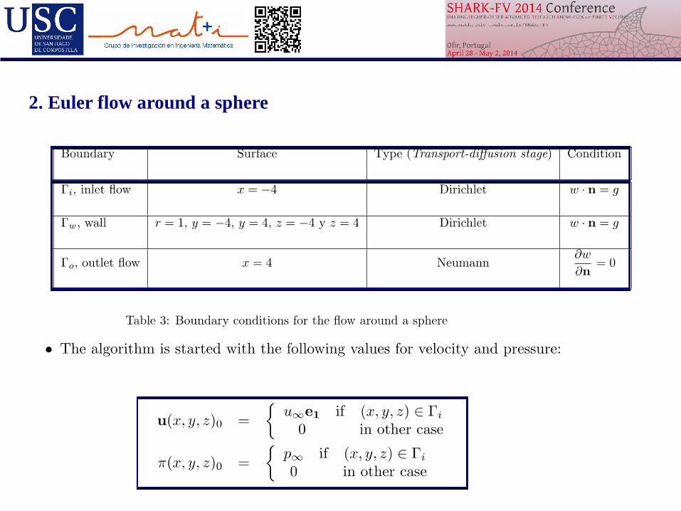
2. Euler flow around a sphere

• 318684 tetrahedra, • 55022 vertices• 641149 finite volumes

The mesh M employed

Finite volume mesh section in z = 0

Steady state

• ∆t = 0.45 the numerical method is unstable • The computer code was written in Fortran 90 and ran on a node of a cluster with a processor Intel Xeon CPU X5570@2.93GHz

2. Euler flow around a sphere

Streamlines and pressure contours on the sphere

p

w

∆t=0.2at t=10

2. Euler flow around a sphere

w pZ=0 ∆t=0.2at t=10

Numerical Results Academic test for Navier-Stokes equations

Errors E(w) (left) and E(p) (right) obtained setting the time step to t =4.88E-4

The explicit discretization

The semi-implicit discretization

The semi-implicit discretization

First Order Rusanov Velocity

Explicito-Cea CFL VELVIS Error M1 last dt Error M2 last dt Error M3 last dtErrorM1/errorM2 ErrorM2/errorM3 Order

Err t final 7,00E+00 8,42E-02 1,63E-02 3,94E-02 5,02E-03 2,00E-02 1,89E-03 2,14E+00 1,97E+00 1,095 0,980

Err t final 5,00E+00 8,42E-02 1,17E-02 3,95E-02 4,14E-03 2,00E-02 2,13E+00 1,97E+00 1,093 0,980

Err t final 4,00E+00 8,42E-02 9,32E-03 3,95E-02 3,31E-03 2,00E-02 1,08E-03 2,13E+00 1,97E+00 1,092 0,981

Err t final 3,00E+00 8,43E-02 7,00E-03 3,96E-02 2,48E-03 2,00E-02 8,09E-04 2,13E+00 1,97E+00 1,091 0,981

Err t final 2,00E+00 8,43E-02 4,67E-03 3,96E-02 1,66E-03 2,01E-02 5,39E-04 2,13E+00 1,97E+00 1,090 0,981

Err l2 tiempo 2,00E+00 4,68E-02 4,67E-03 2,14E-02 1,66E-03 1,01E-02 5,39E-04 2,18E+00 2,12E+00 1,127 1,087

Pressure

CFL VELVIS Error M1 Error M2 Error M3ErrorM1/errorM2 ErrorM2/errorM3 Order

Err t final 7,00E+00 1,74E-01 7,56E-02 4,22E-02 2,30E+00 1,79E+00 1,199 0,843

Err t final 5,00E+00 1,78E-01 8,04E-02 4,36E-02 2,21E+00 1,84E+00 1,145 0,883

Err t final 4,00E+00 1,73E-01 8,73E-02 4,31E-02 1,98E+00 2,03E+00 0,986 1,018

Err t final 3,00E+00 1,73E-01 7,84E-02 4,39E-02 2,21E+00 1,78E+00 1,146 0,835

Err t final 2,00E+00 1,74E-01 8,12E-02 4,39E-02 2,15E+00 1,85E+00 1,103 0,888

Err l2 tiempo 2,00E+00 8,46E-02 3,94E-02 2,17E-02 2,15E+00 1,81E+00 1,104 0,856

Orden2 Cea-Vc convectivo

Explicito-CeaVC Viscosidad Velocity

CFL VELVIS Error M1 last dt Error M2 last dt Error M3 last dtErrorM1/errorM2 ErrorM2/errorM3 Order

Err t final 7,00E+00 9,15E-02 1,63E-02 3,15E-02 5,81E-03 1,25E-02 1,89E-03 2,91E+00 2,52E+00 1,540 1,333

Err L2 tiempo 7,00E+00 7,39E-02 1,84E-02 7,10E-03 4,01E+00 2,60E+00 2,003 1,377

Pressure

CFL VELVIS Error M1 Error M2 Error M3 ErrorM1/errorM2 Order

Err t final 7,00E+00 1,28E-01 3,09E-02 1,19E-02 4,139059963 2,59E+00 1,373 1,373

Err L2 tiempo 7,00E+00 6,54E-02 1,78E-02 6,56E-03 3,67E+00 2,71E+00 1,441 1,441Orden2 convectivo + viscosidad

Explicito-Ce Viscosidad Velocidad

CFL VELVIS Error M1 Last dt Error M2 DT VV tfinal-1 Error M3Last dt ErrorM1/

errorM2 ErrorM2/errorM3Order

Err t final 7,00E+00 1,25E-01 1,69E-02 4,43E-02 5,83E-03 1,87E-02 1,89E-03 2,81E+00 2,89E+00 1,491 1,531

Err L2 tiempo 7,00E+00 8,46E-02 2,46E-02 9,75E-03 3,44E+00 2,52E+00 1,782 1,336

Err t final 2,00E+00 1,23E-01 4,80E-03 4,34E-02 1,67E-03 1,86E-02 5,41E-04 2,84E+00 2,34E+00 1,507 1,225

Err L2 tiempo 2,00E+00 6,47E-02 2,41E-02 9,71E-03 2,69E+00 2,48E+00 1,426 1,311

Pressure

CFL VELVIS Error M1 Error M2 Error M3ErrorM1/errorM2 ErrorM2/errorM3

Order

Err t final 7,00E+00 1,44E-01 5,42E-02 3,21E-02 2,66E+00 1,69E+00 1,409 0,754

Err L2 tiempo 7,00E+00 7,84E-02 2,69E-02 1,59E-02 2,91E+00 1,70E+00 1,542 0,762

Err t final 2,00E+00 1,37E-01 4,84E-02 3,07E-02 2,83E+00 1,58E+00 1,500 0,659

Err L2 tiempo 2,00E+00 6,66E-02 2,36E-02 9,71E-03 2,82E+00 2,43E+00 1,494 1,283

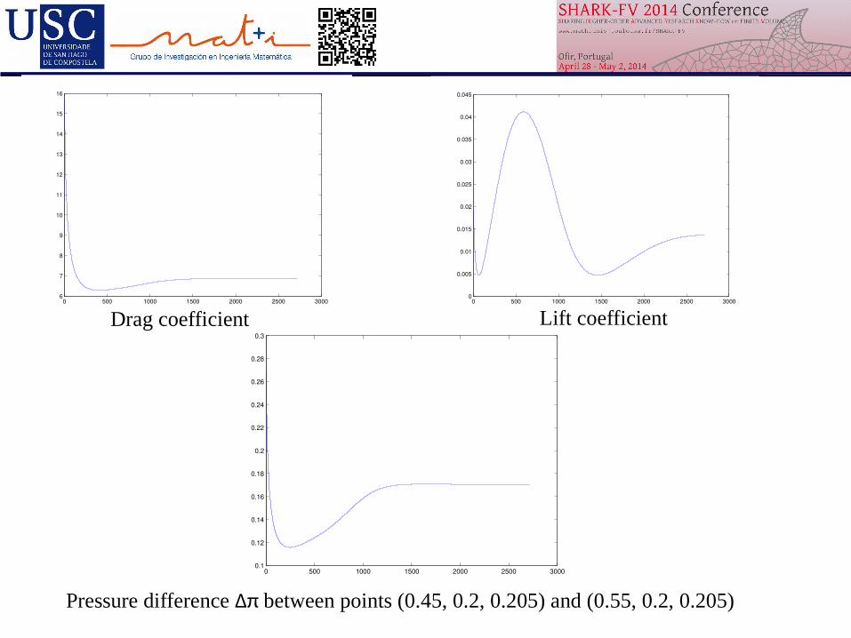
3. Flow around a cylinder

Approximated wx at z=0

Approximated pressure at z=0

Streamlines

Q-Scheme of van Leer (T1) and Rusanov (T2). 2nd Order Cea-VC method.

0 500 1000 1500 2000 2500 30006

7

8

9

10

11

12

13

14

15

16

0 500 1000 1500 2000 2500 30000

0.005

0.01

0.015

0.02

0.025

0.03

0.035

0.04

0.045

0 500 1000 1500 2000 2500 30000.1

0.12

0.14

0.16

0.18

0.2

0.22

0.24

0.26

0.28

0.3

Drag coefficient Lift coefficient

Pressure difference ∆π between points (0.45, 0.2, 0.205) and (0.55, 0.2, 0.205)

Low-Mach number equations with transport and energy equations

Test with a transport equation: Gaussian sphere

L. Saavedra (2012)

Conclusions

• The transport-diffusion stage is done by a time-explicit face finite volume discretization

on a unstructured mesh, upwinded by classical approximate Riemann solvers.

• The projection stage consists of boundary-value problem for the Laplace operator that is

solved by a standard finite element method. • The use of face-type finite volumes facilitates the imposition of flux boundary conditions

and leads to a staggered-like spatial discretization of velocity and pressure.• In the case of steady-state problems a semi-implicit discretization is also proposed for

the viscous term allowing for larger time steps than those needed for the fully explicit

scheme.

• The method is applied to several different test problems allowing us to assess its

accuracy. In general, first order is achieved, both in time and in space.

• Since the transport-diffusion stage is explicit in time and the matrix for the projection

stage can be factorized only once because it is time independent, the overall method is

cheap. Moreover, the transport-diffusion stage can be easily parallelized leading to a

considerable improvement in the computational efficiency.

Obrigada!

elena.vazquez-cendon@usc.es