Embed Size (px)
Citation preview
FLORIDA STATE UNIVERSITY
COLLEGE OF ENGINEERING
A GRAPH BASED APPROACH TO NONLINEAR MODEL PREDICTIVE CONTROL WITH
APPLICATION TO COMBUSTION CONTROL AND FLOW CONTROL
By
BRANDON M. REESE
A Dissertation submitted to theDepartment of Mechanical Engineering
in partial fulfillment of therequirements for the degree of
Doctor of Philosophy
Degree Awarded:Spring Semester, 2015
Copyright c© 2015 Brandon M. Reese. All Rights Reserved.

Brandon M. Reese defended this dissertation on April 2, 2015.The members of the supervisory committee were:
Emmanuel G. Collins
Professor Co-Directing Dissertation
Farrukh S. Alvi
Professor Co-Directing Dissertation
Simon Y. Foo
University Representative
Louis N. Cattafesta
Committee Member
William S. Oates
Committee Member
The Graduate School has verified and approved the above-named committee members, and certifies that thedissertation has been approved in accordance with university requirements.
ii

ACKNOWLEDGMENTS
I would like to acknowledge my family and friends, my CISCOR and FCAAP Colleagues, the McKnight
Doctoral Fellowship Program, the GEM Consortium Fellowship, the Army Research Office, the National
Science Foundation, and the Army Research Laboratory. Without the support, funding, opportunities, and
encouragement offered to me from each of these, I would not have been able to complete this dissertation
and degree.
iii
TABLE OF CONTENTS
List of Tables . . . . . . . . . . . . . . . . . . . . . . . . . . . . . . . . . . . . . . . . . . . . . . . vi
List of Figures . . . . . . . . . . . . . . . . . . . . . . . . . . . . . . . . . . . . . . . . . . . . . . . vii
List of Symbols . . . . . . . . . . . . . . . . . . . . . . . . . . . . . . . . . . . . . . . . . . . . . . xiii
Abstract . . . . . . . . . . . . . . . . . . . . . . . . . . . . . . . . . . . . . . . . . . . . . . . . . . xv
1 Research Objective 11.1 Motivation . . . . . . . . . . . . . . . . . . . . . . . . . . . . . . . . . . . . . . . . . . . . 11.2 Problem Statement . . . . . . . . . . . . . . . . . . . . . . . . . . . . . . . . . . . . . . . 21.3 Dissertation Contributions . . . . . . . . . . . . . . . . . . . . . . . . . . . . . . . . . . . 3
2 Background and Literature Review 42.1 Nonlinear Model Predictive Control . . . . . . . . . . . . . . . . . . . . . . . . . . . . . . 42.2 Predictive Optimization . . . . . . . . . . . . . . . . . . . . . . . . . . . . . . . . . . . . . 42.3 Neural Network Identification . . . . . . . . . . . . . . . . . . . . . . . . . . . . . . . . . 52.4 Power Plant Combustion . . . . . . . . . . . . . . . . . . . . . . . . . . . . . . . . . . . . 72.5 Flow Separation . . . . . . . . . . . . . . . . . . . . . . . . . . . . . . . . . . . . . . . . . 8
2.5.1 Nonlinear POD Methods . . . . . . . . . . . . . . . . . . . . . . . . . . . . . . . . 82.5.2 Recent Advances in Active Flow Control . . . . . . . . . . . . . . . . . . . . . . . 92.5.3 Actuation for Flow Control . . . . . . . . . . . . . . . . . . . . . . . . . . . . . . . 102.5.4 The Need for an Improved Performance Function . . . . . . . . . . . . . . . . . . . 10
3 Adaptive SBMPC 123.1 Methodology . . . . . . . . . . . . . . . . . . . . . . . . . . . . . . . . . . . . . . . . . . 12
3.1.1 The MRAN Identification Network . . . . . . . . . . . . . . . . . . . . . . . . . . 123.1.2 Sampling Based Model Predictive Optimization . . . . . . . . . . . . . . . . . . . . 16
3.2 Simulation and Results . . . . . . . . . . . . . . . . . . . . . . . . . . . . . . . . . . . . . 203.2.1 Identification Comparison . . . . . . . . . . . . . . . . . . . . . . . . . . . . . . . 223.2.2 Control Comparison . . . . . . . . . . . . . . . . . . . . . . . . . . . . . . . . . . 233.2.3 Run Time Statistics and Real Time Feasibility . . . . . . . . . . . . . . . . . . . . . 24
3.3 Summary . . . . . . . . . . . . . . . . . . . . . . . . . . . . . . . . . . . . . . . . . . . . 25
4 Application to Combustion Control 284.1 Introduction . . . . . . . . . . . . . . . . . . . . . . . . . . . . . . . . . . . . . . . . . . . 284.2 Combustion Plant and Neural Network Identification . . . . . . . . . . . . . . . . . . . . . 29
4.2.1 Description of the Plant . . . . . . . . . . . . . . . . . . . . . . . . . . . . . . . . 294.2.2 Neural Network Identification . . . . . . . . . . . . . . . . . . . . . . . . . . . . . 314.2.3 Neural Network Tuning . . . . . . . . . . . . . . . . . . . . . . . . . . . . . . . . 32
4.3 Control Results . . . . . . . . . . . . . . . . . . . . . . . . . . . . . . . . . . . . . . . . . 334.3.1 Case 1: Time-Invariant SISO Problem . . . . . . . . . . . . . . . . . . . . . . . . . 344.3.2 Case 2: Introducing a Carbon Penalty Cost . . . . . . . . . . . . . . . . . . . . . . 34
iv
4.3.3 Case 3: Control System Adaptation Under Changing Dynamics . . . . . . . . . . . 404.3.4 Run Time Statistics and Real Time Feasibility . . . . . . . . . . . . . . . . . . . . . 444.3.5 Tuning the Control Algorithms . . . . . . . . . . . . . . . . . . . . . . . . . . . . . 45
4.4 Summary . . . . . . . . . . . . . . . . . . . . . . . . . . . . . . . . . . . . . . . . . . . . 45
5 Application to Flow Separation Control 475.1 Introduction . . . . . . . . . . . . . . . . . . . . . . . . . . . . . . . . . . . . . . . . . . . 47
5.1.1 Control Objective . . . . . . . . . . . . . . . . . . . . . . . . . . . . . . . . . . . . 485.2 Control Method . . . . . . . . . . . . . . . . . . . . . . . . . . . . . . . . . . . . . . . . . 49
5.2.1 Sampling the Input Domain . . . . . . . . . . . . . . . . . . . . . . . . . . . . . . 505.2.2 The Graph Search . . . . . . . . . . . . . . . . . . . . . . . . . . . . . . . . . . . 505.2.3 Nonlinear Modelling . . . . . . . . . . . . . . . . . . . . . . . . . . . . . . . . . . 51
5.3 Formulation of Lift Based Performance Function . . . . . . . . . . . . . . . . . . . . . . . 535.3.1 Lift Based Performance Function Validation Results . . . . . . . . . . . . . . . . . 57
5.4 Experiments and Results . . . . . . . . . . . . . . . . . . . . . . . . . . . . . . . . . . . . 635.4.1 Flow Control Experimental Setup . . . . . . . . . . . . . . . . . . . . . . . . . . . 655.4.2 Particle Image Velocimetry . . . . . . . . . . . . . . . . . . . . . . . . . . . . . . . 665.4.3 Open-Loop Characterization . . . . . . . . . . . . . . . . . . . . . . . . . . . . . . 675.4.4 Closed-Loop Control . . . . . . . . . . . . . . . . . . . . . . . . . . . . . . . . . . 75
5.5 Summary . . . . . . . . . . . . . . . . . . . . . . . . . . . . . . . . . . . . . . . . . . . . 82
6 Concluding Remarks 866.1 Summary of Completed Research . . . . . . . . . . . . . . . . . . . . . . . . . . . . . . . 866.2 Future Work . . . . . . . . . . . . . . . . . . . . . . . . . . . . . . . . . . . . . . . . . . . 87
6.2.1 Learning of Heuristics . . . . . . . . . . . . . . . . . . . . . . . . . . . . . . . . . 876.2.2 Parallel Implementation . . . . . . . . . . . . . . . . . . . . . . . . . . . . . . . . 876.2.3 Additional Applications . . . . . . . . . . . . . . . . . . . . . . . . . . . . . . . . 876.2.4 Future Flow Control Research . . . . . . . . . . . . . . . . . . . . . . . . . . . . . 88
Appendices
A SBMPO Algorithm Pseudocode 90
B SBMPO Soundness and Completeness Proof 92
C Lists of Simulation and Experiment Parameters 94
D List of Tuning Parameter Choices 96
E Lift Based Performance Function Plots 100
Bibliography . . . . . . . . . . . . . . . . . . . . . . . . . . . . . . . . . . . . . . . . . . . . . . . 106
Biographical Sketch . . . . . . . . . . . . . . . . . . . . . . . . . . . . . . . . . . . . . . . . . . . . 112
v
LIST OF TABLES
3.1 Adaptive SBMPC Run Time Statistics: Case 1 . . . . . . . . . . . . . . . . . . . . . . . . . 24
4.1 Time Variation of Simulation Plant Dynamics . . . . . . . . . . . . . . . . . . . . . . . . . . 40
4.2 Adaptive SBMPC Run Time Statistics . . . . . . . . . . . . . . . . . . . . . . . . . . . . . . 44
5.1 Chord Locations of Microjet exits and Transducers. . . . . . . . . . . . . . . . . . . . . . . . 66
C.1 Simulation Parameters: Combustion . . . . . . . . . . . . . . . . . . . . . . . . . . . . . . . 94
C.2 Experiment Parameters: Flow Control . . . . . . . . . . . . . . . . . . . . . . . . . . . . . . 95
D.1 MRAN Parameter Choices: Combustion Control . . . . . . . . . . . . . . . . . . . . . . . . 96
D.2 BPN Parameter Choices . . . . . . . . . . . . . . . . . . . . . . . . . . . . . . . . . . . . . 97
D.3 SBMPC Parameter Choices: Combustion Control . . . . . . . . . . . . . . . . . . . . . . . . 97
D.4 GPC Parameter Choices: Combustion Control . . . . . . . . . . . . . . . . . . . . . . . . . . 98
D.5 MRAN Parameter Choices: Flow Control . . . . . . . . . . . . . . . . . . . . . . . . . . . . 98
D.6 SBMPC Parameter Choices: Flow Control . . . . . . . . . . . . . . . . . . . . . . . . . . . . 99
vi

LIST OF FIGURES
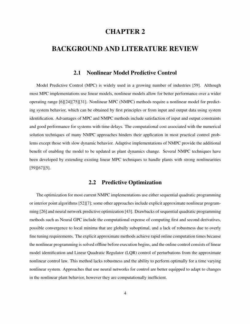
2.1 The layout of a sample RBF network consists of a hidden layer containing one hidden neuronfor each distinct state pattern that the algorithm encounters. Collectively these pattern statevectors make up a basis with which all system dynamics are modelled. With enough of thesehidden neurons the network is able to match arbitrarily complex nonlinear behavior. . . . . . 6
3.1 Block Diagram of Adaptive SBMPC. The control task is to provide inputs u to the plant suchthat outputs y match a reference trajectory r. The neural network model is identified online,and as candidate input trajectories u∗ are provided by SBMPO to the neural network, theircorresponding predicted outputs y∗ are returned. . . . . . . . . . . . . . . . . . . . . . . . . . 13
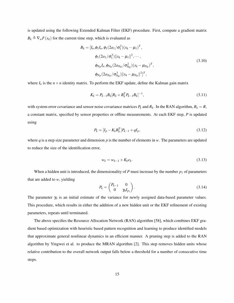
3.2 Minimal Resource Allocation Network Flowchart. The MRAN algorithm learns the numberof hidden units needed to represent the system and continually refines the parameters of eachhidden unit. . . . . . . . . . . . . . . . . . . . . . . . . . . . . . . . . . . . . . . . . . . . . 14
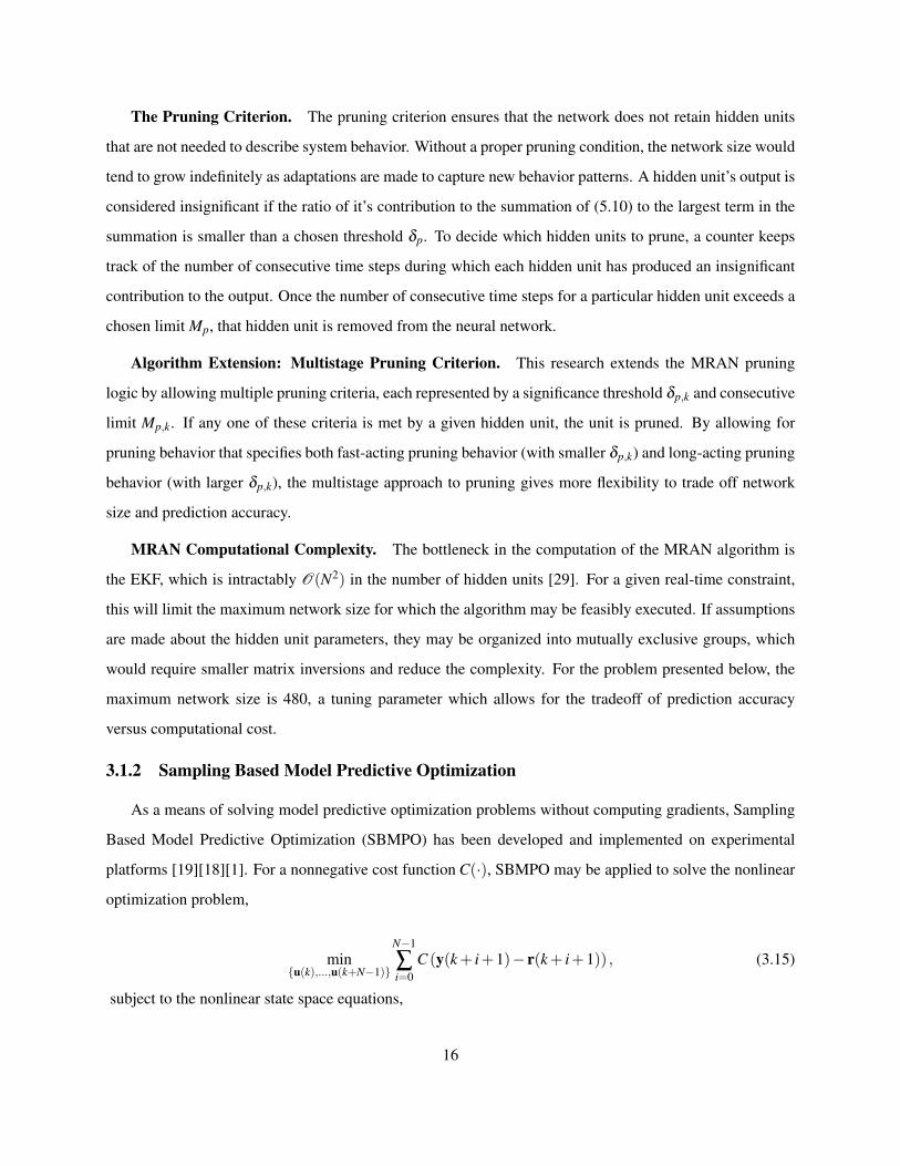
3.3 Sampling Based Model Predictive Optimization Summary. The algorithm discretizes the in-put space and makes model-based state predictions, xk+ j, in order to minimize a cost function. 17
3.4 SBMPO Search Graph. The graph is built by expanding the most promising node to generateB child nodes. Each child node is assigned an input sample, which is propagated forwardthrough the model to predict a state for that node. The potential cost of reaching that state isused to prioritize the nodes and select the most promising candidate for the next iteration ofexpansion. . . . . . . . . . . . . . . . . . . . . . . . . . . . . . . . . . . . . . . . . . . . . . 19
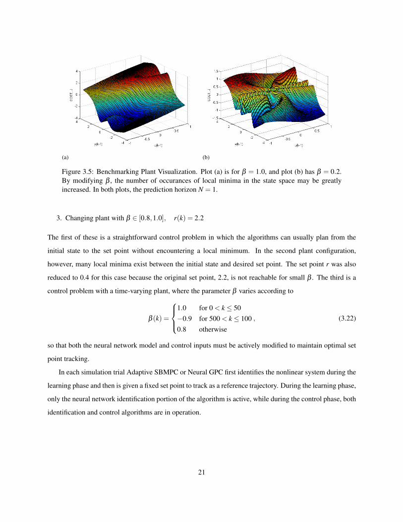
3.5 Benchmarking Plant Visualization. Plot (a) is for β = 1.0, and plot (b) has β = 0.2. Bymodifying β , the number of occurances of local minima in the state space may be greatlyincreased. In both plots, the prediction horizon N = 1. . . . . . . . . . . . . . . . . . . . . . 21
3.6 Training Phase Prediction Errors. Though the BPN algorithm is able to execute each itera-tion more quickly, completing 25 times more iterations than the RBF learning algorithm, thelatter converges much faster and produces lower prediction errors throughout the 30-secondlearning phase. . . . . . . . . . . . . . . . . . . . . . . . . . . . . . . . . . . . . . . . . . . 22
3.7 Case 1 Results—β = 1.0 step tracking. After a 30-second training phase, the reference wastracked using GPC (a) and SBMPC (b). Both converge rapidly to the desired set point andachieve steady state estimation and control errors of zero. In the error plot (c), tracking erroris the absolute percent difference between desired and actual outputs, while prediction erroris the absolute percent difference between predicted and actual outputs. . . . . . . . . . . . . 23
3.8 Case 2 Results—β = 0.2 step tracking. After a 90-second training phase, the reference wastracked using GPC (a) and SBMPC (b). Both converge more slowly than in the previous case.However Neural GPC convergence takes 100 simulation steps while the Adaptive SBMPCmethod converges within 20 steps. The GPC suboptimal convergence state is due to finding a
vii
local minimum. The error plot (c) indicates a difference of 2.5 orders of magnitude betweenglobally optimal convergence of SBMPC and the locally optimal convergence of GPC. . . . . 26
3.9 Case 3 Results—Variable β step tracking. After a 30-second training phase, the referencewas tracked using GPC (a) and SBMPC (b). Both converge rapidly to the desired set pointand achieve low errors, maintaining good performance as the plant dynamics undergo abruptchanges at time steps 50 and 100. The error plot (c) indicates that Adaptive SBMPC convergesmore quickly than Neural GPC in response to these changes. . . . . . . . . . . . . . . . . . . 27
4.1 Single Output Neural Network ID comparison. Each neural network is trained with sequentialinput and output data during the training phase. Prediction error is based only on predictionof xO2. . . . . . . . . . . . . . . . . . . . . . . . . . . . . . . . . . . . . . . . . . . . . . . . 31
4.2 Multiple Output Neural Network ID comparison. Identification error is computed based onpredictions for the three outputs, xO2, xCO, xCO2. For this case, the BPN adaptation convergesmore slowly, but two identification methods eventually attain comparable prediction error. . . 32
4.3 Case 1 Results—Step Tracking.The reference input was tracked using Neural GPC (a), SBMPCRBF
(b), and SBMPCBPN (c). The neural network type affects overshoot due to larger BPN pre-diction errors. SBMPC convergence, however, is still more rapid than that of GPC regardlessof neural network choice. . . . . . . . . . . . . . . . . . . . . . . . . . . . . . . . . . . . . . 35
4.4 Neural GPC Case 2 Results. Penalties on CO and CO2 are introduced and plots of inputsdampler angle (a) and fuel rate (b), and outputs oxygen concentration (c) and carbon dioxideconcentration (d) are given. The shaded upper and lower regions on the input plots are infea-sible regions beyond the input constraints. The value u2,SAT is input to the plant when the fuelrate constraint violation occurs. . . . . . . . . . . . . . . . . . . . . . . . . . . . . . . . . . 37
4.5 SBMPCRBF Case 2 Results. The performance of Adaptive SBMPC is shown. Plots of inputsdampler angle (a) and fuel rate (b), and outputs oxygen concentration (c) and carbon diox-ide concentration (d) are given. The shaded upper and lower regions on the input plots areinfeasible regions beyond the input constraints. . . . . . . . . . . . . . . . . . . . . . . . . . 38
4.6 SBMPCBPN Case 2 Results. The performance of SBMPC using BPN identification is shown.Plots of inputs dampler angle (a) and fuel rate (b), and outputs oxygen concentration (c) andcarbon dioxide concentration (d) are given. The shaded upper and lower regions on the inputplots are infeasible regions beyond the input constraints. . . . . . . . . . . . . . . . . . . . . 39
4.7 Neural GPC Case 3 Results. With plant changes occuring every 500 seconds, the modeladapts and control inputs are updated simultaneously. Plots of inputs dampler angle (a) andfuel rate (b), and outputs oxygen concentration (c) and carbon dioxide concentration (d) aregiven. The shaded upper and lower regions on the input plots are infeasible regions beyond theinput constraints. The value u2,SAT is input to the plant when the fuel rate constraint violationoccurs. . . . . . . . . . . . . . . . . . . . . . . . . . . . . . . . . . . . . . . . . . . . . . . 41
4.8 SBMPCRBF Case 3 Results. SBMPCRBF adapts to the plant changes at 500 second intervals.Plots of inputs dampler angle (a) and fuel rate (b), and outputs oxygen concentration (c) and
viii
carbon dioxide concentration (d) are given. The shaded upper and lower regions on the inputplots are infeasible regions beyond the input constraints. . . . . . . . . . . . . . . . . . . . . 42
4.9 SBMPCBPN Case 3 Results. SBMPCBPN adapts to the plant changes at 500 second intervals.Plots of inputs dampler angle (a) and fuel rate (b), and outputs oxygen concentration (c) andcarbon dioxide concentration (d) are given. The shaded upper and lower regions on the inputplots are infeasible regions beyond the input constraints. . . . . . . . . . . . . . . . . . . . . 43
5.1 Sampling Based Model Predictive Control Summary. The algorithm discretizes the inputspace and makes model-based state predictions, xk+ j, in order to minimize a cost function. . . 49
5.2 SBMPC Search Graph. The graph is built by expanding the most promising node to generateB child nodes. Each child node is assigned an input sample, which is propagated forwardthrough the model to predict a state for that node. The potential cost of reaching that state isused to prioritize the nodes and select the most promising candidate for the next iteration ofexpansion. . . . . . . . . . . . . . . . . . . . . . . . . . . . . . . . . . . . . . . . . . . . . . 50
5.3 The layout of a sample RBF network consists of a hidden layer containing one hidden neuronfor each distinct state pattern that the algorithm encounters. Collectively these pattern statevectors make up a basis with which all system dynamics are modeled. With enough of thesehidden neurons the network is able to match arbitrarily complex nonlinear behavior. . . . . . 52
5.4 XFOIL Simulation of NACA 0025, 6 degrees, Re = 100,000. . . . . . . . . . . . . . . . . . . 54
5.5 Airfoil Microjet Array and Pressure Transducer Schematic. . . . . . . . . . . . . . . . . . . . 55
5.6 Percent errors when angle approximation α = αsep is used. . . . . . . . . . . . . . . . . . . . 57
5.7 Vli f t for lower Reynolds numbers, evaluated from simualated pressures. . . . . . . . . . . . . 58
5.8 Vli f t for transitional Reynolds numbers, evaluated from simualated pressures. . . . . . . . . . 59
5.9 Vli f t for higher Reynolds numbers, evaluated from simualated pressures. . . . . . . . . . . . . 60
5.10 Lift Coefficient and L/D for Re = 90000 (a) and Re = 100000 (b). . . . . . . . . . . . . . . . 61
5.11 Assembled Airfoil CAD with Pressure Transducers . . . . . . . . . . . . . . . . . . . . . . . 62
5.12 Zli f t evaluated with measured pressures compared to measured lift for Re=95,000. . . . . . . 63
5.13 Measured lift and negative prms evaluated with a single measured pressure signal for Re=95,000. 64
5.14 Airfoil Schematic. This diagram includes the locations of microjet array M1 and M2 andpressure transducers P1 though P4. . . . . . . . . . . . . . . . . . . . . . . . . . . . . . . . . 65
5.15 Buffer Circuit Diagram . The buffer circuit amplifies an input voltage signal so that the outputvoltage has sufficient current to drive the solenoid valves. . . . . . . . . . . . . . . . . . . . . 66
ix
5.16 PIV Experiment Photograph. The PIV setup takes snapshot images of illuminated smokeparticles. Processing the images yields velocity field measurements. The laser and opticalhardware are configured to illuminate only the smoke particles in the desired plane. . . . . . . 67
5.17 Time Domain Channel Pressures during Pulsed Actuation. The phase-averaged response ofthe actuator to a 12 Hz square wave is plotted. The width and delay computations are calcu-lated at half of the maximum height of the waveform. . . . . . . . . . . . . . . . . . . . . . . 68
5.18 Frequency Domain Channel Pressures during Pulsed Actuation. The response of the actuatorto frequency inputs is plotted.This plot displays the response measured at the microjet channelfor several different source pressures P0. . . . . . . . . . . . . . . . . . . . . . . . . . . . . . 69
5.19 Exit Pressures during Pulsed Actuation. The pressures measured at the microjet exit displaya similar trend to those measured within the channel; however, because of the low signal-to-noise ratio, the data for a 10 PSI source pressure is plotted. . . . . . . . . . . . . . . . . . . . 70
5.20 Zli f t Response to Frequency Actuation at AOA = 19.8◦. For various flow conditions, themajority of the lift improvement occurs from 0 to 80 Hz. This is consistent with findingsfrom bandwidth tests, which indicated that 80 Hz was the highest frequency to which thevalves are capable of responding. . . . . . . . . . . . . . . . . . . . . . . . . . . . . . . . . 71
5.21 Zli f t response to frequency actuation at AOA = 22.0◦. Open loop results at a different angleof attack indicate a clearly nonlinear relationship between input frequency and Zli f t . . . . . . 72
5.22 Measured cp Values at Pressure Transducer Locations. The pressure transducers are posi-tioned to resolve the suction peak, which grows in each case due to frequency actuation.Larger suction peaks generally correspond to increased overall lift. . . . . . . . . . . . . . . . 74
5.23 Closed Loop Case 1. The Reynolds number is 125,000, and the angle of attack is 20◦. Thisclosed loop case illustrates ability to follow a step reference signal subsequent to the activationof the SBMPC controller. . . . . . . . . . . . . . . . . . . . . . . . . . . . . . . . . . . . . . 77
5.24 Closed Loop Case 2. The Reynolds number is 125,000, and the angle of attack is 20◦. Thisclosed loop case illustrates the ability to command intermediate vales of Zli f t . . . . . . . . . . 78
5.25 Closed Loop Case 3. The Reynolds number is 125,000, and the angle of attack is 20◦. Thisclosed loop case illustrates the saturation behavior of the controller: from time 0 to 5 seconds,Zli f t is simply maximized when the specified reference is above the attainable actuation range.Tracking resumes when the reference value is decreased to an attainable value. . . . . . . . . 79
5.26 Closed Loop Case 4. The Reynolds number is 150,000, and the angle of attack is 20◦. Thisclosed loop case illustrates the ability to track ramp trajectories. During training, the tunnelReynolds number was set to 125,000, ensuring that online model adaptation would be requiredwhen tested at a higher Reynolds number. . . . . . . . . . . . . . . . . . . . . . . . . . . . . 80
5.27 Closed Loop Case 5. The Reynolds number shifts from 150,000 to 140,000, and the angle ofattack is 20◦. This case demonstrates that the ability to adapt enables the control system to berobust to changes in the flow conditions. . . . . . . . . . . . . . . . . . . . . . . . . . . . . . 81
x

5.28 Baseline (a) and Controlled (b) Vx for 16◦, 15 m/s. The baseline PIV data was collected withthe control system off. In the controlled case, data was collected with the control system setto maximize Zli f t , and the tunnel speed corresponds to a Reynolds number of 150,000 basedon chord length. . . . . . . . . . . . . . . . . . . . . . . . . . . . . . . . . . . . . . . . . . . 82
5.29 Baseline (a) and Controlled (b) Vx for 16◦, 12 m/s. The baseline PIV data was collected withthe control system off. In the controlled case, data was collected with the control system setto maximize Zli f t , and the tunnel speed corresponds to a Reynolds number of 125,000 basedon chord length. . . . . . . . . . . . . . . . . . . . . . . . . . . . . . . . . . . . . . . . . . . 83
5.30 Baseline (a) and Controlled (b) Vx for 16◦, 15 m/s. The baseline PIV data was collected withthe control system off. In the controlled case, data was collected with the control system setto maximize Zli f t , and the tunnel speed corresponds to a Reynolds number of 90,000 basedon chord length. . . . . . . . . . . . . . . . . . . . . . . . . . . . . . . . . . . . . . . . . . . 83
5.31 Baseline (a) and Controlled (b) Vx for 22◦, 11 m/s. The baseline PIV data was collected withthe control system off. In the controlled case, data was collected with the control system setto maximize Zli f t , and the tunnel speed corresponds to a Reynolds number of 90,000 basedon chord length. . . . . . . . . . . . . . . . . . . . . . . . . . . . . . . . . . . . . . . . . . . 84
5.32 Baseline (a) and Controlled (b) Vx for 22◦, 12 m/s. The baseline PIV data was collected withthe control system off. In the controlled case, data was collected with the control system setto maximize Zli f t , and the tunnel speed corresponds to a Reynolds number of 125,000 basedon chord length. . . . . . . . . . . . . . . . . . . . . . . . . . . . . . . . . . . . . . . . . . . 84
5.33 Baseline (a) and Controlled (b) Vx for 22◦, 15 m/s. The baseline PIV data was collected withthe control system off. In the controlled case, data was collected with the control system setto maximize Zli f t , and the tunnel speed corresponds to a Reynolds number of 150,000 basedon chord length. . . . . . . . . . . . . . . . . . . . . . . . . . . . . . . . . . . . . . . . . . . 85
E.1 Lift Coefficient and L/D for Re = 50000. . . . . . . . . . . . . . . . . . . . . . . . . . . . . 100
E.2 Lift Coefficient and L/D for Re = 60000. . . . . . . . . . . . . . . . . . . . . . . . . . . . . 101
E.3 Lift Coefficient and L/D for Re = 70000. . . . . . . . . . . . . . . . . . . . . . . . . . . . . 101
E.4 Lift Coefficient and L/D for Re = 80000. . . . . . . . . . . . . . . . . . . . . . . . . . . . . 102
E.5 Lift Coefficient and L/D for Re = 90000. . . . . . . . . . . . . . . . . . . . . . . . . . . . . 102
E.6 Lift Coefficient and L/D for Re = 100000. . . . . . . . . . . . . . . . . . . . . . . . . . . . 103
E.7 Lift Coefficient and L/D for Re = 110000. . . . . . . . . . . . . . . . . . . . . . . . . . . . 103
E.8 Lift Coefficient and L/D for Re = 120000. . . . . . . . . . . . . . . . . . . . . . . . . . . . 104
E.9 Lift Coefficient and L/D for Re = 130000. . . . . . . . . . . . . . . . . . . . . . . . . . . . 104
E.10 Lift Coefficient and L/D for Re = 140000. . . . . . . . . . . . . . . . . . . . . . . . . . . . 105
xi

E.11 Lift Coefficient and L/D for Re = 150000. . . . . . . . . . . . . . . . . . . . . . . . . . . . 105
xii

LIST OF SYMBOLS
The following list contains symbols used throughout the document.
x Vector of statesy Vector of sensor outputsy Vector of Predicted outputsu Vector of actuator inputsT Control period
RBF Radial Basis FunctionBPN Back Propagation Network
φ j jth hidden unit activation functionµ j jth hidden unit centroid vectorσ j jth hidden unit widtha j jth hidden unit output layer weight vectore1 Instantaneous prediction errore2 RMS prediction errore3 Euclidean distance from nearest centroidM RMS window sizeE1 Instantaneous prediction error thresholdE2 RMS prediction error thresholdE3 Euclidean distance from nearest centroid threshold
δp,k kth pruning thresholdMp,k kth pruning window
NH Number of hidden unitsL BPN Network GainB Branchout factorN Prediction horizon
Nc Control Horizonα Learning rateη Momentum coefficientε Solver tolerances Constraint sharpness
λ Damping factor
xiii

xO2 Oxygen concentrationxCO2 Carbon dioxide concentrationxCO Carbon monoxide concentrationφ Air flow damper angleΦ Air inlet flow [kg/s]Φ f Fuel inlet flow [kg/s]c Chord length [inches]b Span length [inches]RE Chord based Reynolds numberAOA Angle of attackCL Lift coefficientCD Drag coefficientZli f t Lift Performance FunctionV∞ Free stream velocity
xiv

ABSTRACT
Systems with a priori unknown, and time-varying dynamic behavior pose a significant challenge in the field
of Nonlinear Model Predictive Control (NMPC). When both the identification of the nonlinear system and
the optimization of control inputs are done robustly and efficiently, NMPC may be applied to control such
systems. This dissertation presents a novel method for adaptive NMPC, called Adaptive Sampling Based
Model Predictive Control (SBMPC), that combines a radial basis function neural network identification
algorithm with a nonlinear optimization method based on graph search. Unlike other NMPC methods, it does
not rely on linearizing the system or gradient based optimization. Instead, it discretizes the input space to the
model via pseudo-random sampling and feeds the sampled inputs through the nonlinear model, producing
a searchable graph. An optimal path is found using an efficient graph search method. Adaptive SBMPC is
used in simulation to identify and control a simple plant with clearly visualized nonlinear dynamics. In these
simulations, both fixed and time-varying dynamic systems are considered. Next, a power plant combustion
simulation demonstrates successful control of a more realistic Multiple-Input Multiple-Output system. The
simulated results are compared with an adaptive version of Neural GPC, an existing NMPC algorithm based
on Netwon-Raphson optimization and a back propagation neural network model. When the cost function
exhibits many local minima, Adaptive SBMPC is successful in finding a globally optimal solution while
Neural GPC converges to a solution that is only locally optimal. Finally, an application to flow separation
control is presented with experimental wind tunnel results. These results demonstrate real time feasibility,
as the control updates are computed at 100 Hz, and highlight the robustness of Adaptive SBMPC to plant
changes and the ability to adapt online. The experiments demonstrate separation control for a NACA 0025
airfoil with Reynolds Numbers ranging from 90,000 to 150,000 for both fixed and pitching (.33 deg/s) angles
of attack.
xv

CHAPTER 1
RESEARCH OBJECTIVE
1.1 Motivation
Model Predictive Control (MPC) has been heavily researched and applied across several industries [60],
especially in the process control industry. Few Adaptive MPC techniques have been developed [52], and the
develpment of practical adaptive MPC methods that use nonlinear models is considered an open problem.
The introduction of an efficient nonlinear adaptive method for MPC would significantly expand the range
applications for which MPC is effective.
The understanding of nonlinear systems is key to solving numerous engineering problems. Along the
path to understanding these systems and solving relevant problems, identification and control methods that
capture and harness nonlinear behavior are necessary. To address problems of this sort, the proposed method,
Adaptive Sampling Based Model Predictive Control (Adaptive SBMPC), was developed. The development
of this nonlinear MPC method has culminated in the research focus of this dissertation. The unique opti-
mization algorithm, Sampling Based Model Predictive Optimization (SBMPO), has been applied in con-
junction with an adaptive, neural-network-based model in order to perform adaptive nonlinear MPC in a
more practical and effective manner than existing methods.
A first implementation of Adaptive SBMPC solved a simple single-input, single-output (SISO) nonlinear
example from the literature. This example served to demonstrate several properties of the approach, namely
the ability to avoid convergence to a local minimum and handle a time-varying plant. A theoretical proof for
the completeness of the proposed method is given. The results for this simplified example help us understand
the identification and control algorithms’ behavior while practical results contribute to real world problem
solving. Two problems of considerable practical significance are addressed in this dissertation: the first
is a power plant combustion control problem investigated by simulation, and the second is a problem of
boundary layer separation control investigated by wind tunnel experiments.
The power plant combustion problem was the first application of Adaptive SBMPC and involves the
immediately relevant competing objectives of efficient power generation and environmental sustainability.
Constraints on inputs and outputs are critical in this industry and MPC techniques are often selected for
1
their ability to satisfy these types of constraints. This simulation illustrates the capability to control a time-
varying nonlinear plant and demonstrates the robustness added by using model adaptation. Furthermore,
results will show the avoidance of locally optimal but globally suboptimal solutions. For comparison, an
existing method, Neural GPC, is implemented and is shown to converge to a local minimum. Multiple-Input
Multiple-Output (MIMO) results are obtained for the combustion control simulation.
The second practical application, control of flow separation, is investigated experimentally using hard-
ware and real time feedback. As boundary layers along aerodynamic surfaces separate in active flight, the
phenomenon of flow separation hampers the performance of rotary and fixed wing aircraft. Wings, tails,
rotor blades, turbomachinery blades, and the fuselage itself are subject to stall, introducing losses and un-
desirable unsteadiness. While passive techniques achieve limited mitigation of separation effects in some
applications, there is a growing need for active control methods that are able to handle diverse and chang-
ing flow conditions. Flows with Reynolds numbers on the order of 100,000 are transitional and are more
susceptible to separation than flows in either laminar or turbulent regimes. Systems that employ existing
passive or active control techniques are able to produce some delay or mitigation of separation effects, but a
new adaptive approach is necessary to maximize performance and recover system losses under the realistic
variation in operating conditions experienced in flight.
1.2 Problem Statement
The primary objective of this research is to develop, implement, and demonstrate a new Nonlinear Model
Predictive Control (NMPC) method. The development of this method includes the specification of the algo-
rithm and some theoretical analysis of the behavior and performance of the algorithm, the implementation
includes the programming of this method for simulation and experimental use. Finally, the demonstration
consists of results of the application of this algorithm in simulation and in experiments. Performance and
computational cost comparisons to the best existing Adaptive NMPC method, Neural GPC, are provided.
The procedures as well as the tuning values used to accomplish these tasks are recorded so that the results
obtained here may be reproduced.
This dissertation develops a control system for general application to systems that could include nonlin-
earity and time dependent behavior. The following are included in the scope of this dissertation. The neces-
sary software design includes simulation implementations, online nonlinear system identification algorithm
implementations, and closed-loop control algorithm implementatinos. Experiments with wind tunnel hard-
2

ware in the loop require the design and construction of an experimental platform for flow separation control.
Next, analysis of the simulated test results allow for comparison with stated objectives and previously pub-
lished adaptive model predictive control methods. Finally, the experimental results must be analyzed to
determine the effectiveness of the presented method when applied to a real flow separation control problem.
1.3 Dissertation Contributions
The research in this dissertation makes unique contributions in the areas of MPC and flow control by
being the first to publish the achievements listed below.
1. Apply the SBMPO graph search and RBF neural network identification methods to perform recedinghorizon NMPC.
(a) First to perform adaptive NMPC using a neural network model that can change its structure aswell as its parameter values.
(b) First to present NMPC results for a time-varying plant.
(c) Theoretically demonstrate the soundness and completeness of SBMPO.
2. Experimentally demonstrate flow separation control with robustness to changing flow conditions.
(a) First to implement NMPC method for real time flow control.
(b) Demonstrate robustness to Reynolds number and angle of attack changes.
3
CHAPTER 2
BACKGROUND AND LITERATURE REVIEW
2.1 Nonlinear Model Predictive Control
Model Predictive Control (MPC) is widely used in a growing number of industries [59]. Although
most MPC implementations use linear models, nonlinear models allow for better performance over a wider
operating range [6][24][75][31]. Nonlinear MPC (NMPC) methods require a nonlinear model for predict-
ing system behavior, which can be obtained by first principles or from input and output data using system
identification. Advantages of MPC and NMPC methods include satisfaction of input and output constraints
and good performance for systems with time delays. The computational cost associated with the numerical
solution techniques of many NMPC approaches hinders their application in most practical control prob-
lems except those with slow dynamic behavior. Adaptive implementations of NMPC provide the additional
benefit of enabling the model to be updated as plant dynamics change. Several NMPC techniques have
been developed by extending existing linear MPC techniques to handle plants with strong nonlinearities
[59][67][5].
2.2 Predictive Optimization
The optimization for most current NMPC implementations use either sequential quadratic programming
or interior point algorithms [52][7]; some other approaches include explicit approximate nonlinear program-
ming [26] and neural network predictive optimization [43]. Drawbacks of sequential quadratic programming
methods such as Neural GPC include the computational expense of computing first and second derivatives,
possible convergence to local minima that are globally suboptimal, and a lack of robustness due to overly
fine tuning requirements. The explicit approximate methods achieve rapid online computation times because
the nonlinear programming is solved offline before execution begins, and the online control consists of linear
model identification and Linear Quadratic Regulator (LQR) control of perturbations from the approximate
nonlinear control law. This method lacks robustness and the ability to perform optimally for a time varying
nonlinear system. Approaches that use neural networks for control are better equipped to adapt to changes
in the nonlinear plant behavior, however they are computationally inefficient.
4

The most notable neural network control method, Adaptive Predictive Control employs the Levenberg-
Marquardt algorithm to learn its neural network parameters. This variant of nonlinear least squares is re-
ported to be computationally expensive and a barrier to online implementation [43]. NMPC, although theo-
retically suitible for particular applications such as flow control, has been considered impractical because of
the computational cost associated with traditional techniques. For this reason, none of the NMPC methods
mentioned above in this section have been successfully implemented in a real time flow control experiments.
In his book Reduced Order Modelling for Flow Control, Noack writes that “even without contraints, a huge
numerical burden will be involved in nonlinear MPC. Today, this is still a limiting factor for flow control
applications” [54]. The proposed approach to adaptive NMPC, Adaptive Sampling Based Model Predic-
tive Control (Adaptive SBMPC), first presented in [64], uses the optimization technique known a Sampling
Based Model Predictive Optimization. This approach is unique from other methods used for NMPC because
the optimization is done by performing a graph search on a sampled input space. This method is explored in
this dissertation with an emphasis on achieving the computational efficiency to solve problems in real time.
2.3 Neural Network Identification
The use of an artificial neural network allows nonlinear models to be identified in a general manner by
composing a function that computes future outputs based on past states. For this application the state vector,
xk = (yTk−1,y
Tk−2, ...,y
Tk−ny
,uTk−1,u
Tk−2, ...,u
Tk−nu
)T , (2.1)
consists of nu prior plant inputs and ny outputs. The form,
yk = f (yk−1,yk−2, ...,yk−ny ,uk−1,uk−2, ...,uk−nu)≡ F(xk), (2.2)
is known as as a nonlinear autoregressive exogenous inputs (NARX) model form because it is analogous
to the autoregressive exogenous inputs (ARX) form for linear models. If F(xk) were a linear function, the
equation would simplify to an ARX formulation,
yk = Axk, (2.3)
with the matrix A of constant coefficients.
5
Figure 2.1: The layout of a sample RBF network consists of a hidden layer containing one hiddenneuron for each distinct state pattern that the algorithm encounters. Collectively these patternstate vectors make up a basis with which all system dynamics are modelled. With enough of thesehidden neurons the network is able to match arbitrarily complex nonlinear behavior.
While there are many ways to construct the nonlinear function F(xk), neural network methods construct
this function as a composition of simpler functions called neural units, which can be arranged in series and
parallel to form a network.
A widely used neural network technique is the Back Propagation Network (BPN) [30]. This method
requires a priori specification of the network size and number of layers and performs parameter updates
using an iterative update rule called back propagation. Since its introduction, many BPN variants have
been proposed, such as recurrent versions of BPN [57] and the addition particle swarm optimization to the
back propagation approach [74]. A disadvantage of BPN-type methods is their fixed structure. Each of the
algorithms listed below are initialized with no neural units and are able to adapt their structure by learning
the suitable number of units to represent the behavior of the system.
The General Regression Neural Network (GRNN) [69] and the Resource Allocation Network (RAN)
[58] both use Radial Basis Function (RBF) neural network structures, depicted in Fig. 2.1, typically having
Gaussian activation functions. Major differences between the two include the EKF parameter optimization
used by RAN, which contrasts to the simpler update rule utilized for GRNN, and the larger parameter space
of RAN. The RAN algorithm fits a separate width to each Gaussian unit while GRNN assumes a common
width for each of its Gaussian units.
The network implemented in this research comes from an extension [73] of the RAN method by Platt.
This Minimal Resource Allocation Network (MRAN), like RAN, has for its first layer a collection of neural
6
units that respond in parallel when the state xk is nearby (according to the Euclidean norm) to a previously
seen pattern. This method adds to RAN a pruning strategy, which ensures that the model retains only the
hidden neurons which have recently contributed significantly to the model output.
2.4 Power Plant Combustion
Energy policy and the rising cost of fossil fuels has highlighted the need for efficient and reliable methods
to control the combustion processes of power plants. Legislation that taxes or sets limits on carbon emissions
is becoming more common [46][61][3], which has increased demand for control systems that reliably meet
constraints on emissions outputs.
When controlling a combustion system, constraints on inputs and outputs are necessary in order to meet
power demands, ensure safe operating levels, or regulate environmental pollutants. For these reasons, the
industry’s need for handling these constraints has steadily increased, and Model Predictive Control (MPC) is
arguably the control methodology most suitable to handle them [51]. MPC uses an internal model that rep-
resents the system to be controlled, and produces a future sequence of control inputs and the corresponding
output trajectory that optimizes a cost function, subject to constraints on functions of the inputs and outputs.
Receding horizon MPC approaches use this model to predict several steps in the future while implementing
only the immediate next step.
MPC is commonly applied in simulations to power plants [9][47][38][23], and, for applications where
no closed-form model is available, is typically applied in conjunction with an identified system model.
Linear MPC techniques often use a Least-Squares, Gradient Descent, or Newton method to fit a linear
model to observed data [59]. Nonlinear MPC techniques, which are far less commonly used, often fit
a Neural Network, Neuro-Fuzzy, Nonlinear Polynomial, or other Nonlinear State Space model to predict
system behavior [60].
Due to environmental effects, normal wear, and fatigue, power plant combustion chambers can exhibit
time-dependent dynamic behavior. The neural network model form is suitable for modeling the nonlin-
earities and time variation, which lead to suboptimal performance when they are ignored. The Neural
Generalized Predictive Control (Neural GPC) method [67][27] consists of a Back Propagation Neural Net-
work (BPN) and Newton-Raphson cost optimization. It is best able to handle problems with nonlinearities
and time variation among existing NMPC methods because it balances speed of optimization with adaptive
capability.
7

An analytical model for coal combustion has been derived [8]. This model has been used in a Single-
Input Single-Output (SISO) simulation of Gaussian Process NMPC [25], which requires a priori specifi-
cation of the plant’s dynamic equations and achieves rapid online computational speed, at the expense of
significant offline computation and a lack of robustness to plant changes. This research in this dissertation
solves the problem that was investigated in [25] using an adaptive algorithm that does not require prior
knowledge other than the order of plant dynamics. Furthermore, the control problem is extended to include
multiple inputs and outputs and time-varying plant dynamics.
2.5 Flow Separation
For decades, flow separation has been of particular interest in engineering applications where improved
aerodynamic performance is desired. Control of flow separation, both active and passive, is a key component
of existing aviation technology. Passive control methods, such as leading edge surface roughness or the
inclusion of vortex generators, rely on a stationary structural component to produce a reduction or delay
in separation effects. These techniques typically produce an early transition to turbulence or streamwise
vortical structures, each of which have been shown to mitigate separation [40]. The effectiveness of passive
techniques is limited in comparison with active techniques, which rely on powered mechanisms to alter
the flow, especially when conditions off the design point are considered [10]. These types of off-design
conditions are common for aircraft that perform maneuvers, micro-aerial vehicles, and aeronautical systems
that are deployed in diverse environments.
Previous adaptive flow separation research has aimed to capture the nonlinear dynamics of the flowfield
by identifying an instantaneously linearized model that varies with time. The optimization of a linear model
has the advantages of speed and simplicity over those that consider nonlinear models. The unmodelled
dynamics, however, can cause such techniques to be suboptimal and even unstable.
2.5.1 Nonlinear POD Methods
Proper Orthogonal Decomposition (POD) techniques have been used to identify models in the form of
polynomial difference equations [65][36] that are sufficient for open loop control design [50]. However, due
to computational expense, closed loop flow control implementations have been limited to linear models. The
primary advantage of SBMPO over alternative methods is that the optimization phase does not prefer linear
to nonlinear models, and the algorithm does not need to compute closed-form gradients. Although SBMPO
8
has the ability to optimize inputs to a POD model, POD models are steady state in nature and do not capture
the transient behavior or hysteresis effects that are necessary to control aerodynamic flows at relevant time
scales.
2.5.2 Recent Advances in Active Flow Control
The significant increase in capability and decrease in cost of computing hardware has led to the fea-
sibility of active control techniques of increasing sophistication. Both open-loop and closed-loop control
schemes have been applied to flow control problems and there is evidence that closed loop approaches offer
significant improvement in performance over open-loop control [55][34].
The linear method Generalized Predictive Control (GPC) [13] as well as ARMARKOV adaptive control
[72] have been effective when applied to the problem of separation flow control [71]. GPC is, in fact, an
implementation of receding horizon model predictive control (MPC) that uses closed-form expressions to
compute the input sequence. Although many passive and open loop control approaches to the problem of
flow separation have been examined, relatively few closed-loop separation control systems have been studied
and successfully implemented. This recent work by Tian et al., is the first to incorporate a sophisticated
adaptive control approach, implementing ARMARKOV online system identification and the ARMARKOV
adaptive disturbance rejection algorithm. Their paper only presents results for stationary and very limited
flow parameters: only one Reynolds number and one fixed angle of attack. More recent work presents
performance for multiple angles of attack; however, each experimental trial is still conducted at a stationary
angle [71]. Since the ARMARKOV and GPC control optimizations rely on closed-form expressions, they
are very difficult, if not impossible, to generalize to nonlinear systems unless the dynamics are linearized.
Using linearization techniques, GPC has been extended to nonlinear systems using neural network models.
These extensions have yet to be applied for flow control although they have been applied in other nonlinear
applications both in simulation and experimentally.
Several areas of flow control research, including suppression of cavity flow resonant tones and mitiga-
tion of flow separation, have advanced rapidly in recent years as new technologies have both created demand
for and expanded the capabilities of such systems. The study of cavity flow control has demonstrated that
mathematical techniques such as Proper Orthogonal Decomposition (POD) and model reduction are effec-
tive tools for controlling aerodynamic systems [50][20]. While these studies incorporated flow visualization
and analysis efforts to produce nonlinear models that are effective for developing open-loop control strate-
9
gies, it has been more practical to linearize these models for the sake of computational efficiency when
implementing real-time closed loop control [55][34].
The problem of flow separation overlaps with the study of cavity flow; frequency domain methods are
applied to model and control the flow dynamics in both applications [49][12][42]. POD methods similar to
those applied to cavity flow have also been used for flow separation [22]. Actuator development has also
been key to the recent advances in the field of flow separation control. Both synthetic jet unsteady actu-
ators [71][70] and steady microjet actuators [12][4] have been effective in separation control experiments.
Because of the advantage of high momentum capability with low power requirements [41], microjets have
been selected as the primary actuators for this research.
2.5.3 Actuation for Flow Control
While the innovations outlined in this dissertation may be applied to many sensor and actuator hardware
configurations, microjet actuators have been selected for this research. Microjet actuators have distinct ad-
vantages over alternatives actuation methods for the control of flow separation. This study will use microjets
capable of steady actuation; however, the control system will also be able to supply unsteady input signal
when a capable actuator is installed. While other micro actuators are able to produce comparable jet veloci-
ties, ease of fabrication and in-house expertise make microjet actuators a practical choice. After proving the
control system concept with microjets, other actuators may easily be interchanged for comparison.
Piezoelectric synthetic jets, another common flow control actuator, while having the advantage of zero
net mass flux, are known to have difficulty generating the mass flow rates and jet speed required for higher
speed applications [4]. Newly developed plasma based thermal actuators have difficulties similar to those
of synthetic jets and tend to take longer to alter the flow [53]. Non-thermal plasma based actuators are in
development but are not as mature and have not achieved the control authority of microjet actuators. At this
point, microjets provide the greatest control authority per unit of power consumption, but it is possible that
still more efficient actuators may be available in the next few years.
2.5.4 The Need for an Improved Performance Function
Previous flow separation control research has used an RMS pressure value as the performance function
for feedback control [71][70][68]. While minimizing prms at a particular transducer location will sometimes
maximize the desired quantity CL/CD, Sheplak et al. present results where at different flow conditions,
control that maximizes CL/CD produces an increase in prms [66]. This result gives evidence that minimizing
10

prms at a single sensor is insufficient for effective control across a wide range of flow conditions. As derived
in [62], a performance function that incorporates several pressure transducer signals and correlates with
CL/CD will make effective closed-loop performance possible over a wider range of angle of attack and
Reynolds number conditions. Since combining multiple transducer signals in an intelligent manner collapses
multiple variables into one performance variable, this method will also reduce the computational effort
needed to perform system identification and control with multiple sensors.
11

CHAPTER 3
ADAPTIVE SBMPC
3.1 Methodology
The Adaptive SBMPC approach to nonlinear MPC consists of identification of an approximate system
model during the learning phase followed by simultaneous identification and control during the control
phase. As shown in Fig. 3.1, a neural network is used to model the plant dynamics and SBMPC is used to
generate actuation signals to control the plant. A summary of the MRAN identification algorithm and the
details of the SBMPC methodology is described below, a full description of the MRAN algorithm may be
found in [2].
3.1.1 The MRAN Identification Network
The Minimal Resource Allocation Network (MRAN) algorithm implemented in this research was de-
veloped by Yingwei et al. [2]. It is based on the Resource Allocation Network algorithm, a general method
for function approximation [58]. The advantage over other methods is that the network eventually reaches
a constant size despite increasing the length of the training set. Yingwei et al. extended RAN to MRAN
by adding a pruning step. The MRAN learning paradigm is sufficiently general to represent many different
systems with little or no alteration of the algorithm’s tuning parameters.
The RBF Neural Network. Referring to Fig. 3.2, MRAN is a general purpose procedure for function
approximation that aims to represent some vector output f (x) as the result of some nonlinear mapping of
the input state vector x. When applying MRAN to learn a system’s input-output behavior, x is the vector of
the past m inputs and n outputs given by
x = [yTi−1,y
Ti−2, ...,y
Ti−n,u
Ti−1,u
Ti−2, ...,u
Ti−m]
T , (3.1)
and f (x) is the current output prediction given by
f (x) = y = a0 +NH
∑j=1
a jφ j(x). (3.2)
12
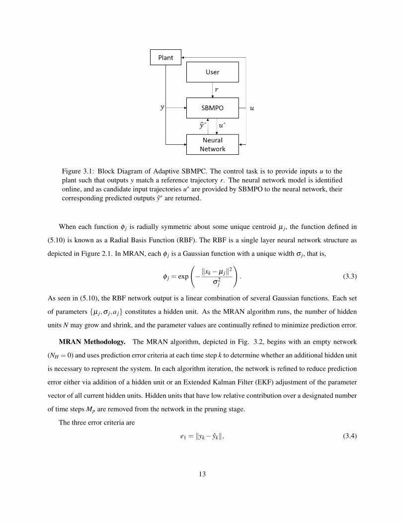
Figure 3.1: Block Diagram of Adaptive SBMPC. The control task is to provide inputs u to theplant such that outputs y match a reference trajectory r. The neural network model is identifiedonline, and as candidate input trajectories u∗ are provided by SBMPO to the neural network, theircorresponding predicted outputs y∗ are returned.
When each function φ j is radially symmetric about some unique centroid µ j, the function defined in
(5.10) is known as a Radial Basis Function (RBF). The RBF is a single layer neural network structure as
depicted in Figure 2.1. In MRAN, each φ j is a Gaussian function with a unique width σ j, that is,
φ j = exp
(−‖xk−µ j‖2
σ2j
). (3.3)
As seen in (5.10), the RBF network output is a linear combination of several Gaussian functions. Each set
of parameters {µ j,σ j,a j} constitutes a hidden unit. As the MRAN algorithm runs, the number of hidden
units N may grow and shrink, and the parameter values are continually refined to minimize prediction error.
MRAN Methodology. The MRAN algorithm, depicted in Fig. 3.2, begins with an empty network
(NH = 0) and uses prediction error criteria at each time step k to determine whether an additional hidden unit
is necessary to represent the system. In each algorithm iteration, the network is refined to reduce prediction
error either via addition of a hidden unit or an Extended Kalman Filter (EKF) adjustment of the parameter
vector of all current hidden units. Hidden units that have low relative contribution over a designated number
of time steps Mp are removed from the network in the pruning stage.
The three error criteria are
e1 = ‖yk− yk‖, (3.4)
13
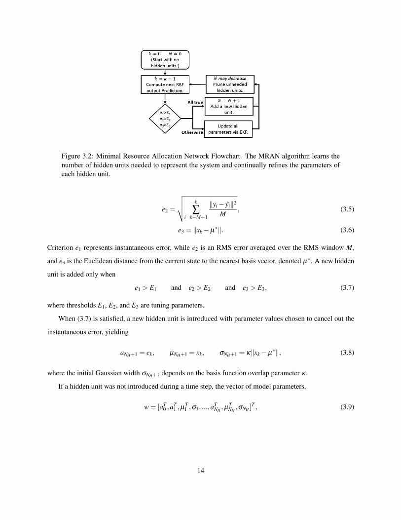
Figure 3.2: Minimal Resource Allocation Network Flowchart. The MRAN algorithm learns thenumber of hidden units needed to represent the system and continually refines the parameters ofeach hidden unit.
e2 =
√√√√ k
∑i=k−M+1
‖yi− yi‖2
M, (3.5)
e3 = ‖xk−µ∗‖. (3.6)
Criterion e1 represents instantaneous error, while e2 is an RMS error averaged over the RMS window M,
and e3 is the Euclidean distance from the current state to the nearest basis vector, denoted µ∗. A new hidden
unit is added only when
e1 > E1 and e2 > E2 and e3 > E3, (3.7)
where thresholds E1, E2, and E3 are tuning parameters.
When (3.7) is satisfied, a new hidden unit is introduced with parameter values chosen to cancel out the
instantaneous error, yielding
aNH+1 = ek, µNH+1 = xk, σNH+1 = κ‖xk−µ∗‖, (3.8)
where the initial Gaussian width σNH+1 depends on the basis function overlap parameter κ .
If a hidden unit was not introduced during a time step, the vector of model parameters,
w = [aT0 ,a
T1 ,µ
T1 ,σ1, ...,aT
NH,µT
NH,σNH ]
T , (3.9)
14
is updated using the following Extended Kalman Filter (EKF) procedure. First, compute a gradient matrix
Bk , ∇wF(xk) for the current time step, which is evaluated as
Bk = [In,φ1In,φ1(2a1/σ21 )(xk−µ1)
T ,
φ1(2a1/σ31 )‖xk−µ1‖2, · · · ,
φNH In,φNH (2aNH/σ2NH)(xk−µNH )
T ,
φNH (2aNH/σ3NH)‖xk−µNH‖2]T ,
(3.10)
where In is the n×n identity matrix. To perform the EKF update, define the Kalman gain matrix
Kk = Pk−1Bk[Rk +BTk Pk−1Bk]
−1, (3.11)
with system error covariance and sensor noise covariance matrices Pk and Rk. In the RAN algorithm, Rk = R,
a constant matrix, specified by sensor properties or offline measurements. At each EKF step, P is updated
using
Pk = [Ip−KkBTk ]Pk−1 +qIp, (3.12)
where q is a step size parameter and dimension p is the number of elements in w. The parameters are updated
to reduce the size of the identification error,
wk = wk−1 +Kkek. (3.13)
When a hidden unit is introduced, the dimensionality of P must increase by the number p1 of parameters
that are added to w, yielding
Pk =
(Pk−1 0
0 γ0Ip1
). (3.14)
The parameter γ0 is an initial estimate of the variance for newly assigned data-based parameter values.
This procedure, which results in either the addition of a new hidden unit or the EKF refinement of existing
parameters, repeats until terminated.
The above specifies the Resource Allocation Network (RAN) algorithm [58], which combines EKF gra-
dient based optimization with heuristic based pattern recognition and learning to produce identified models
that approximate general nonlinear dynamics in an efficient manner. A pruning step is added to the RAN
algorithm by Yingwei et al. to produce the MRAN algorithm [2]. This step removes hidden units whose
relative contribution to the overall network output falls below a threshold for a number of consecutive time
steps.
15
The Pruning Criterion. The pruning criterion ensures that the network does not retain hidden units
that are not needed to describe system behavior. Without a proper pruning condition, the network size would
tend to grow indefinitely as adaptations are made to capture new behavior patterns. A hidden unit’s output is
considered insignificant if the ratio of it’s contribution to the summation of (5.10) to the largest term in the
summation is smaller than a chosen threshold δp. To decide which hidden units to prune, a counter keeps
track of the number of consecutive time steps during which each hidden unit has produced an insignificant
contribution to the output. Once the number of consecutive time steps for a particular hidden unit exceeds a
chosen limit Mp, that hidden unit is removed from the neural network.
Algorithm Extension: Multistage Pruning Criterion. This research extends the MRAN pruning
logic by allowing multiple pruning criteria, each represented by a significance threshold δp,k and consecutive
limit Mp,k. If any one of these criteria is met by a given hidden unit, the unit is pruned. By allowing for
pruning behavior that specifies both fast-acting pruning behavior (with smaller δp,k) and long-acting pruning
behavior (with larger δp,k), the multistage approach to pruning gives more flexibility to trade off network
size and prediction accuracy.
MRAN Computational Complexity. The bottleneck in the computation of the MRAN algorithm is
the EKF, which is intractably O(N2) in the number of hidden units [29]. For a given real-time constraint,
this will limit the maximum network size for which the algorithm may be feasibly executed. If assumptions
are made about the hidden unit parameters, they may be organized into mutually exclusive groups, which
would require smaller matrix inversions and reduce the complexity. For the problem presented below, the
maximum network size is 480, a tuning parameter which allows for the tradeoff of prediction accuracy
versus computational cost.
3.1.2 Sampling Based Model Predictive Optimization
As a means of solving model predictive optimization problems without computing gradients, Sampling
Based Model Predictive Optimization (SBMPO) has been developed and implemented on experimental
platforms [19][18][1]. For a nonnegative cost function C(·), SBMPO may be applied to solve the nonlinear
optimization problem,
min{u(k),...,u(k+N−1)}
N−1
∑i=0
C (y(k+ i+1)− r(k+ i+1)) , (3.15)
subject to the nonlinear state space equations,
16
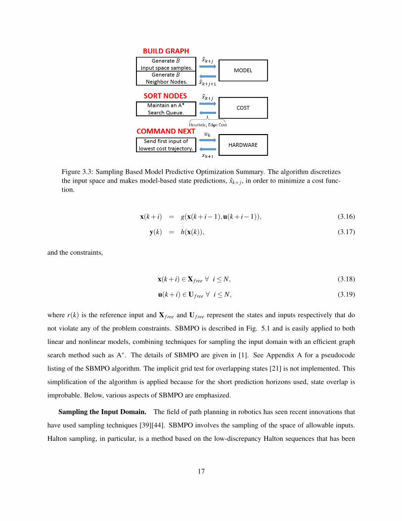
Figure 3.3: Sampling Based Model Predictive Optimization Summary. The algorithm discretizesthe input space and makes model-based state predictions, xk+ j, in order to minimize a cost func-tion.
x(k+ i) = g(x(k+ i−1),u(k+ i−1)), (3.16)
y(k) = h(x(k)), (3.17)
and the constraints,
x(k+ i) ∈ X f ree ∀ i≤ N, (3.18)
u(k+ i) ∈ U f ree ∀ i≤ N, (3.19)
where r(k) is the reference input and X f ree and U f ree represent the states and inputs respectively that do
not violate any of the problem constraints. SBMPO is described in Fig. 5.1 and is easily applied to both
linear and nonlinear models, combining techniques for sampling the input domain with an efficient graph
search method such as A∗. The details of SBMPO are given in [1]. See Appendix A for a pseudocode
listing of the SBMPO algorithm. The implicit grid test for overlapping states [21] is not implemented. This
simplification of the algorithm is applied because for the short prediction horizons used, state overlap is
improbable. Below, various aspects of SBMPO are emphasized.
Sampling the Input Domain. The field of path planning in robotics has seen recent innovations that
have used sampling techniques [39][44]. SBMPO involves the sampling of the space of allowable inputs.
Halton sampling, in particular, is a method based on the low-discrepancy Halton sequences that has been
17

shown to provide representative sample sets consisting of fewer points than sets generated using pseudo-
random numbers or regular grids [56][11]. Satisfaction of input constraints is automatic, since it is the
allowable inputs that are sampled, and since the inputs are propagated forward through the model, no inver-
sion of the model is needed.
The Graph Search. Using the current state and input samples, several nodes are computed by propa-
gating the model and added to a graph with tree connectivity, as illustrated in Fig. 5.2. The branchout factor
B, a tuning parameter of the algorithm, determines how many child nodes are generated when a particular
parent node is expanded. In the implementation of this algorithm, each node has a pointer to its parent node
so that, for every node, there is an implied path from the root node to itself. Therefore, the optimization task
is to choose the node at horizon depth that is reachable by the lowest cumulative cost. The computation is
done by best-first search using the A∗ algorithm [28] or one of its variants such as LPA∗ [37].
SBMPO Completeness. For the receding horizon MPC problem, we define a goal state as any horizon-
depth node whose trajectory is minimal in cost. A sound graph search algorithm returns only trajectory so-
lutions that reach a goal state. A given sound algorithm is complete if it always returns one such solution if
any solution exists. Assuming the heuristic function always underestimates the lowest cost to the prediction
horizon, SBMPO, like A∗ and other graph search algorithms, may be shown to be complete over a given
graph. A proof loosely based on the procedure in [35] is formally derived in Appendix B. Its culmination,
Theorem B.0.6, guarantees that, subject to sufficient depth and breadth of sampling, SBMPO will find a
globally optimal solution. Due to gaps between samples, some suboptimality will result. Note that with the
nonuniform sampling strategy described in Subsection 3.1.2, the gaps between samples become very small
at steady state.
Obstacles and Hard Constraints. Because the input domain samples are selected from the specified
region only, hard input constraints are met automatically. An additional advantage of using a graph search
approach is the ease of dealing with obstacles and hard output constraints. Naturally, if a node represents a
state that is not allowed by the specified constraints or obstacles, it is removed from the queue and the next
node in the queue is chosen instead.
Algorithm Contribution: Precomputed Samples. The Halton sequence algorithm, which is poten-
tially used thousands of times at each time interval when the SBMPC routine is called, was a major contribu-
tor to the total runtime of SBMPC. Generating new Halton samples takes a median of 210 times longer than
18
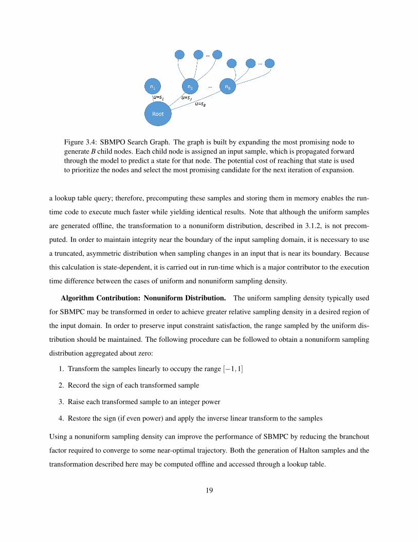
Figure 3.4: SBMPO Search Graph. The graph is built by expanding the most promising node togenerate B child nodes. Each child node is assigned an input sample, which is propagated forwardthrough the model to predict a state for that node. The potential cost of reaching that state is usedto prioritize the nodes and select the most promising candidate for the next iteration of expansion.
a lookup table query; therefore, precomputing these samples and storing them in memory enables the run-
time code to execute much faster while yielding identical results. Note that although the uniform samples
are generated offline, the transformation to a nonuniform distribution, described in 3.1.2, is not precom-
puted. In order to maintain integrity near the boundary of the input sampling domain, it is necessary to use
a truncated, asymmetric distribution when sampling changes in an input that is near its boundary. Because
this calculation is state-dependent, it is carried out in run-time which is a major contributor to the execution
time difference between the cases of uniform and nonuniform sampling density.
Algorithm Contribution: Nonuniform Distribution. The uniform sampling density typically used
for SBMPC may be transformed in order to achieve greater relative sampling density in a desired region of
the input domain. In order to preserve input constraint satisfaction, the range sampled by the uniform dis-
tribution should be maintained. The following procedure can be followed to obtain a nonuniform sampling
distribution aggregated about zero:
1. Transform the samples linearly to occupy the range [−1,1]
2. Record the sign of each transformed sample
3. Raise each transformed sample to an integer power
4. Restore the sign (if even power) and apply the inverse linear transform to the samples
Using a nonuniform sampling density can improve the performance of SBMPC by reducing the branchout
factor required to converge to some near-optimal trajectory. Both the generation of Halton samples and the
transformation described here may be computed offline and accessed through a lookup table.
19

SBMPO Computational Complexity. The execution time required to run SBMPO, the optimization
phase of Adaptive SBMPC, is roughly proportional to the number of nodes expanded, which is the case for
most graph search algorithms [17]. The SBMPO search tree is generated and explored in a best-first sense.
For a maximum graph size of V vertices, SBMPO is an O(|V |) algorithm since, in the worst case, every node
with depth less than the control horizon will be expanded, yielding an upper bound of BN−1 expansions. In
practice, the number required is far fewer, but the worst case is considered when developing a real-time
execution guarantee. While real time algorithms are often programmed to terminate early in the event of
a longer-than-feasible execution time, this can often lead to undesired performance. In the implementation
of SBMPO, the real-time guarantee is achieved by limiting the nodes that may be generated in a single call
of the SBMPO routine. In the event that the optimization phase terminates early, the evaluated nodes of
greatest depth are listed and the node among those with lowest cost is chosen.
3.2 Simulation and Results
For comparison, both Adaptive SBMPC and Neural GPC were used to control the benchmark SISO
nonlinear plant [73] described by the difference equation
y(k) =29β (k)
40sin(
16u(k−1)+8y(k−1)β (k)(3+4u(k−1)2 +4y(k−1)2
)+
15
u(k−1)+15
y(k−1),(3.20)
where β (k) is a parameter that may be modified to alter the behavior of the plant. The MPC cost function,
J =N−1
∑i=0
(y(k+ i+1)− r(k+ i+1))2 , (3.21)
was optimized by each algorithm, equally weighting each future term up to the prediction horizon N. The
SISO, first-order nature of the plant allows simple visualization of the state-to-cost behavior, by plotting the
states u(k−1) and y(k−1) on the lateral axes and the cost (3.21) on the vertical axis. In order to simplify
the visualizations, the cost functions have prediction horizon N = 1. Two versions of the plant are visualized
in Fig. 3.5: (a) β = 1.0 and (b) β = 0.2.
The following three plant cases were considered:
1. Fixed plant with β = 1.0, r(k) = 2.2
2. Fixed plant with β = 0.2, r(k) = 0.4
20
(a) (b)
Figure 3.5: Benchmarking Plant Visualization. Plot (a) is for β = 1.0, and plot (b) has β = 0.2.By modifying β , the number of occurances of local minima in the state space may be greatlyincreased. In both plots, the prediction horizon N = 1.
3. Changing plant with β ∈ [0.8,1.0], r(k) = 2.2
The first of these is a straightforward control problem in which the algorithms can usually plan from the
initial state to the set point without encountering a local minimum. In the second plant configuration,
however, many local minima exist between the initial state and desired set point. The set point r was also
reduced to 0.4 for this case because the original set point, 2.2, is not reachable for small β . The third is a
control problem with a time-varying plant, where the parameter β varies according to
β (k) =
1.0 for 0 < k ≤ 50−0.9 for 500 < k ≤ 1000.8 otherwise
, (3.22)
so that both the neural network model and control inputs must be actively modified to maintain optimal set
point tracking.
In each simulation trial Adaptive SBMPC or Neural GPC first identifies the nonlinear system during the
learning phase and then is given a fixed set point to track as a reference trajectory. During the learning phase,
only the neural network identification portion of the algorithm is active, while during the control phase, both
identification and control algorithms are in operation.
21
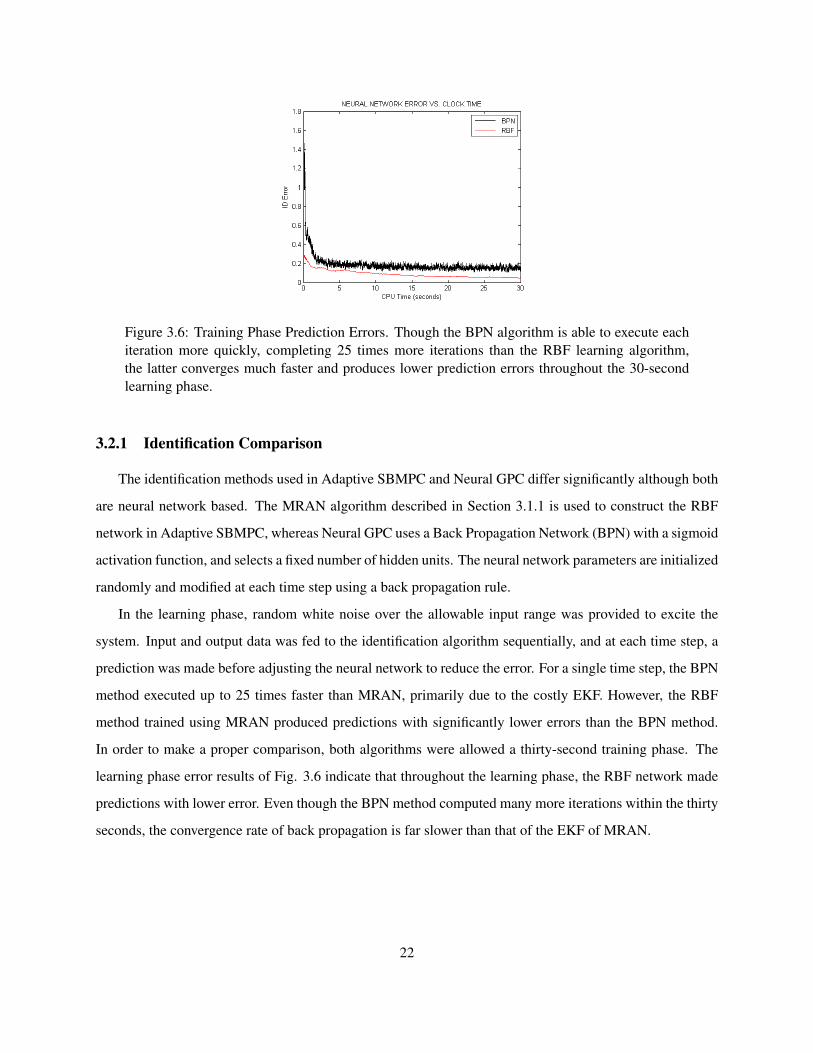
Figure 3.6: Training Phase Prediction Errors. Though the BPN algorithm is able to execute eachiteration more quickly, completing 25 times more iterations than the RBF learning algorithm,the latter converges much faster and produces lower prediction errors throughout the 30-secondlearning phase.
3.2.1 Identification Comparison
The identification methods used in Adaptive SBMPC and Neural GPC differ significantly although both
are neural network based. The MRAN algorithm described in Section 3.1.1 is used to construct the RBF
network in Adaptive SBMPC, whereas Neural GPC uses a Back Propagation Network (BPN) with a sigmoid
activation function, and selects a fixed number of hidden units. The neural network parameters are initialized
randomly and modified at each time step using a back propagation rule.
In the learning phase, random white noise over the allowable input range was provided to excite the
system. Input and output data was fed to the identification algorithm sequentially, and at each time step, a
prediction was made before adjusting the neural network to reduce the error. For a single time step, the BPN
method executed up to 25 times faster than MRAN, primarily due to the costly EKF. However, the RBF
method trained using MRAN produced predictions with significantly lower errors than the BPN method.
In order to make a proper comparison, both algorithms were allowed a thirty-second training phase. The
learning phase error results of Fig. 3.6 indicate that throughout the learning phase, the RBF network made
predictions with lower error. Even though the BPN method computed many more iterations within the thirty
seconds, the convergence rate of back propagation is far slower than that of the EKF of MRAN.
22
3.2.2 Control Comparison
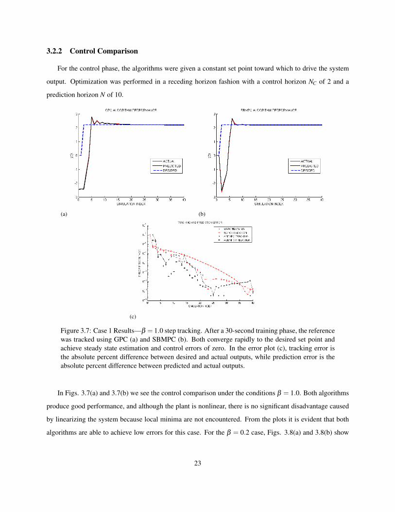
For the control phase, the algorithms were given a constant set point toward which to drive the system
output. Optimization was performed in a receding horizon fashion with a control horizon NC of 2 and a
prediction horizon N of 10.
(a) (b)
(c)
Figure 3.7: Case 1 Results—β = 1.0 step tracking. After a 30-second training phase, the referencewas tracked using GPC (a) and SBMPC (b). Both converge rapidly to the desired set point andachieve steady state estimation and control errors of zero. In the error plot (c), tracking error isthe absolute percent difference between desired and actual outputs, while prediction error is theabsolute percent difference between predicted and actual outputs.
In Figs. 3.7(a) and 3.7(b) we see the control comparison under the conditions β = 1.0. Both algorithms
produce good performance, and although the plant is nonlinear, there is no significant disadvantage caused
by linearizing the system because local minima are not encountered. From the plots it is evident that both
algorithms are able to achieve low errors for this case. For the β = 0.2 case, Figs. 3.8(a) and 3.8(b) show
23

that Neural GPC converges to a suboptimal local minimum and hence fails to track the desired reference,
whereas SBMPC converges to the global minimum and has near zero steady state tracking error. For the
third case, with variable β , both algorithms achieve good performance, tracking the set point as shown in
Figs. 3.7(a) and 3.7(b).
3.2.3 Run Time Statistics and Real Time Feasibility
The computational times presented in Table 4.2 were measured during simulation execution for each of
the three cases. The timing period begins before the SBMPC routine and ends after SBMPC has computed
the next control input. Median and worst case performance over each 200-timestep simulation run are
presented. Both algorithms were implemented in C on a 2.0 GHz quad-core AMD processor.
The Adaptive SBMPC algorithm solves the nonlinear optimization more efficiently than Neural GPC.
In particular, as seen in Table 4.2, it requires far less computational time per step, and as seen in Figs.
3.7(c), 3.8(c), and 3.9(c), it requires fewer time steps to converge to a near-optimal solution. Note that GPC
uses a Newton-Rhaphson method relying on plant linearization while SBMPC is based on a graph search
method that directly propagates the nonlinear plant model and is guaranteed to find the global minimum
given sufficient sampling and sufficient length of the prediction horizon. Hence, SBMPC, unlike GPC, is
not susceptible to slow convergence when the second derivative is small, large overshoot and constraint
violations due to a non-well-behaved first derivative, and non-convergence due to poor initial estimates.
Table 3.1: Adaptive SBMPC Run Time Statistics: Case 1
Median CPU Times
Plant ConfigurationControl Algorithm
GPC SBMPCCase 1 146 MFLOPS 2.67 MFLOPSCase 2 42.0 MFLOPS 4.83 MFLOPSCase 3 148 MFLOPS 2.50 MFLOPS
Longest CPU Times
Plant ConfigurationControl Algorithm
GPC SBMPCCase 1 597 MFLOPS 5.33 MFLOPSCase 2 166 MFLOPS 13.8 MFLOPSCase 3 597 MFLOPS 6.50 MFLOPS
24

3.3 Summary
Adaptive SBMPC, a new approach to adaptive nonlinear model predictive control, is presented and ap-
plied in simulation to a benchmark nonlinear control problem from the literature. The nonlinear dynamics
of the SISO benchmark system were learned and applied in feed-forward control. Efficient nonlinear opti-
mization was performed and close reference tracking was achieved. The SBMPO algorithm for optimization
is shown to be a complete search algorithm subject to sufficient length of the prediction horizon. Unlike ap-
proaches that optimize by linearization, global convergence is achievable even when numerous local minima
exist. For comparison, the established NMPC technique, Neural GPC was also implemented. Through sim-
ulated identification and control problems, adaptive SBMPC was shown to be capable of faster and more
optimal convergence.
Results were presented for a system with fixed as well as changing dynamics, which highlights the
adaptive nature of the control system. One limitation of this and other NMPC approaches is the breakdown
due to complexity for large numbers of inputs and outputs. However, SBMPO is naturally compatible with
parallel computation since it uses a divide-and-conquer approach perform optimization. Node expansion is
the most costly portion of the Adaptive SBMPC algorithm, but these computations can be implemented in
parallel. There is also a possibility for significant computational improvement with the addition of search
heuristics and a parallel implementation of portions of the algorithm. Within an A∗ optimization, a good
heuristic can dramatically reduce the number of nodes that are expanded, and performing the edge cost
calculation in parallel on multiple cores could significantly reduce the required run time per node. Future
work includes the incorporation of learned heuristic functions for problems where no good heuristic is
known based on first principles.
25

(a) (b)
(c)
Figure 3.8: Case 2 Results—β = 0.2 step tracking. After a 90-second training phase, the referencewas tracked using GPC (a) and SBMPC (b). Both converge more slowly than in the previouscase. However Neural GPC convergence takes 100 simulation steps while the Adaptive SBMPCmethod converges within 20 steps. The GPC suboptimal convergence state is due to finding a localminimum. The error plot (c) indicates a difference of 2.5 orders of magnitude between globallyoptimal convergence of SBMPC and the locally optimal convergence of GPC.
26
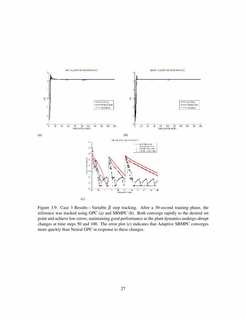
(a) (b)
(c)
Figure 3.9: Case 3 Results—Variable β step tracking. After a 30-second training phase, thereference was tracked using GPC (a) and SBMPC (b). Both converge rapidly to the desired setpoint and achieve low errors, maintaining good performance as the plant dynamics undergo abruptchanges at time steps 50 and 100. The error plot (c) indicates that Adaptive SBMPC convergesmore quickly than Neural GPC in response to these changes.
27
CHAPTER 4
APPLICATION TO COMBUSTION CONTROL
4.1 Introduction
Energy policy and the rising cost of fossil fuels has highlighted the need for efficient and reliable methods
to control the combustion processes of power plants. Legislation that taxes or sets limits on carbon emissions
is becoming more common [46][61][3], which has increased demand for control systems that reliably meet
constraints on emissions outputs.
When controlling a combustion system, constraints on inputs and outputs are necessary in order to meet
power demands, ensure safe operating levels, or regulate environmental pollutants. For these reasons, the
industry’s need for handling these constraints has steadily increased, and Model Predictive Control (MPC) is
arguably the control methodology most suitable to handle them [51]. MPC uses an internal model that rep-
resents the system to be controlled, and produces a future sequence of control inputs and the corresponding
output trajectory that optimizes a cost function, subject to constraints on functions of the inputs and outputs.
Receding horizon MPC approaches use this model to predict several steps in the future while implementing
only the immediate next step.
MPC is commonly applied in simulations to power plants [9][47][38][23], and, for applications where
no closed-form model is available, is typically applied in conjunction with an identified system model.
Linear MPC techniques often use a Least-Squares, Gradient Descent, or Newton method to fit a linear
model to observed data [59]. Nonlinear MPC techniques, which are far less commonly used, often fit
a Neural Network, Neuro-Fuzzy, Nonlinear Polynomial, or other Nonlinear State Space model to predict
system behavior [60].
Due to environmental effects, normal wear, and fatigue, power plant combustion chambers can exhibit
time-dependent dynamic behavior. Furthermore, the addition of solar and wind power plants, which provide
intermittent power to the grid, has caused the duty cycle of traditional power plants to fluctuate more than
ever before. The neural network model form is suitable for modeling the nonlinearities and time variation,
which lead to suboptimal performance when they are ignored. The Neural Generalized Predictive Control
(Neural GPC) method [67][27] consists of a Back Propagation Neural Network (BPN) and Newton-Raphson
28
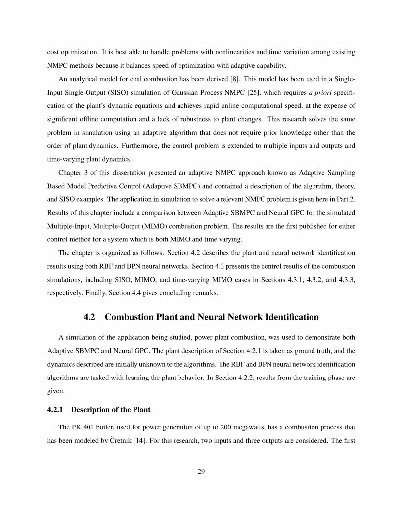
cost optimization. It is best able to handle problems with nonlinearities and time variation among existing
NMPC methods because it balances speed of optimization with adaptive capability.
An analytical model for coal combustion has been derived [8]. This model has been used in a Single-
Input Single-Output (SISO) simulation of Gaussian Process NMPC [25], which requires a priori specifi-
cation of the plant’s dynamic equations and achieves rapid online computational speed, at the expense of
significant offline computation and a lack of robustness to plant changes. This research solves the same
problem in simulation using an adaptive algorithm that does not require prior knowledge other than the
order of plant dynamics. Furthermore, the control problem is extended to multiple inputs and outputs and
time-varying plant dynamics.
Chapter 3 of this dissertation presented an adaptive NMPC approach known as Adaptive Sampling
Based Model Predictive Control (Adaptive SBMPC) and contained a description of the algorithm, theory,
and SISO examples. The application in simulation to solve a relevant NMPC problem is given here in Part 2.
Results of this chapter include a comparison between Adaptive SBMPC and Neural GPC for the simulated
Multiple-Input, Multiple-Output (MIMO) combustion problem. The results are the first published for either
control method for a system which is both MIMO and time varying.
The chapter is organized as follows: Section 4.2 describes the plant and neural network identification
results using both RBF and BPN neural networks. Section 4.3 presents the control results of the combustion
simulations, including SISO, MIMO, and time-varying MIMO cases in Sections 4.3.1, 4.3.2, and 4.3.3,
respectively. Finally, Section 4.4 gives concluding remarks.
4.2 Combustion Plant and Neural Network Identification
A simulation of the application being studied, power plant combustion, was used to demonstrate both
Adaptive SBMPC and Neural GPC. The plant description of Section 4.2.1 is taken as ground truth, and the
dynamics described are initially unknown to the algorithms. The RBF and BPN neural network identification
algorithms are tasked with learning the plant behavior. In Section 4.2.2, results from the training phase are
given.
4.2.1 Description of the Plant
The PK 401 boiler, used for power generation of up to 200 megawatts, has a combustion process that
has been modeled by Cretnik [14]. For this research, two inputs and three outputs are considered. The first
29
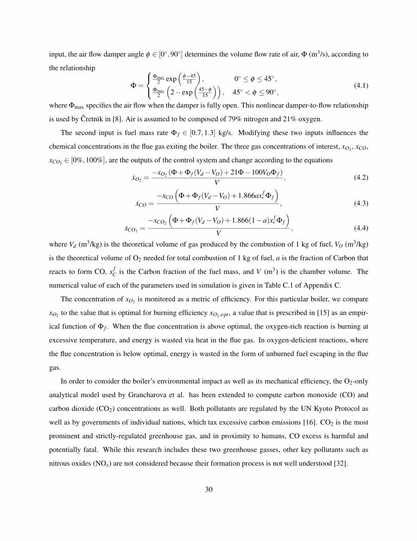
input, the air flow damper angle φ ∈ [0◦,90◦] determines the volume flow rate of air, Φ (m3/s), according to
the relationship
Φ =
Φmax
2 exp(
φ−4515
), 0◦ ≤ φ ≤ 45◦,
Φmax2
(2− exp
(45−φ
15
)), 45◦ < φ ≤ 90◦,
(4.1)
where Φmax specifies the air flow when the damper is fully open. This nonlinear damper-to-flow relationship
is used by Cretnik in [8]. Air is assumed to be composed of 79% nitrogen and 21% oxygen.
The second input is fuel mass rate Φ f ∈ [0.7,1.3] kg/s. Modifying these two inputs influences the
chemical concentrations in the flue gas exiting the boiler. The three gas concentrations of interest, xO2 , xCO,
xCO2 ∈ [0%,100%], are the outputs of the control system and change according to the equations
xO2 =−xO2 (Φ+Φ f (Vd−VO)+21Φ−100VOΦ f )
V, (4.2)
xCO =−xCO
(Φ+Φ f (Vd−VO)+1.866ax f
c Φ f
)V
, (4.3)
xCO2 =−xCO2
(Φ+Φ f (Vd−VO)+1.866(1−a)x f
c Φ f
)V
, (4.4)
where Vd (m3/kg) is the theoretical volume of gas produced by the combustion of 1 kg of fuel, VO (m3/kg)
is the theoretical volume of O2 needed for total combustion of 1 kg of fuel, a is the fraction of Carbon that
reacts to form CO, x fC is the Carbon fraction of the fuel mass, and V (m3) is the chamber volume. The
numerical value of each of the parameters used in simulation is given in Table C.1 of Appendix C.
The concentration of xO2 is monitored as a metric of efficiency. For this particular boiler, we compare
xO2 to the value that is optimal for burning efficiency xO2,opt , a value that is prescribed in [15] as an empir-
ical function of Φ f . When the flue concentration is above optimal, the oxygen-rich reaction is burning at
excessive temperature, and energy is wasted via heat in the flue gas. In oxygen-deficient reactions, where
the flue concentration is below optimal, energy is wasted in the form of unburned fuel escaping in the flue
gas.
In order to consider the boiler’s environmental impact as well as its mechanical efficiency, the O2-only
analytical model used by Grancharova et al. has been extended to compute carbon monoxide (CO) and
carbon dioxide (CO2) concentrations as well. Both pollutants are regulated by the UN Kyoto Protocol as
well as by governments of individual nations, which tax excessive carbon emissions [16]. CO2 is the most
prominent and strictly-regulated greenhouse gas, and in proximity to humans, CO excess is harmful and
potentially fatal. While this research includes these two greenhouse gasses, other key pollutants such as
nitrous oxides (NOx) are not considered because their formation process is not well understood [32].
30
Figure 4.1: Single Output Neural Network ID comparison. Each neural network is trained withsequential input and output data during the training phase. Prediction error is based only onprediction of xO2.
4.2.2 Neural Network Identification
Identification of the nonlinear system dynamics was achieved by training both RBF and BPN neural
network models. The MRAN identification algorithm [73], described in Part 1, was used to train the RBF
network, while the more standard back propagation adaptation rule [76] was used to train the BPN network.
A key distinction between the two identification approaches is that for BPN, a fixed network size must be
assumed, while the RBF adds new hidden units when needed to model newly seen data.
For this simulation, the BPN network was initialized with random parameters for each hidden unit, and
the RBF network was initialized with no hidden units. To determine the network size for the BPN network,
system identification simulations were run with integer network sizes between 1 and 400 hidden units. The
network size of 39 hidden units produced the smallest cumulative error, so this network size was assumed
for the cases presented. The ability to learn the size of the network while the identification algorithm runs is
an advantage of MRAN learning over back propagation.
The simulation was run on one CPU core of a 2.0 GHz quad-core AMD laptop with 6 gigabytes of
RAM. All algorithms were implemented in C.
During neural network training, a sequence of white noise over the allowable range for each input was
provided as the open loop excitation signal. These signals as well as the measured outputs that result from
the inputs were sequentially passed to the identification algorithms. Identical sequences were used for the
31
Figure 4.2: Multiple Output Neural Network ID comparison. Identification error is computedbased on predictions for the three outputs, xO2, xCO, xCO2. For this case, the BPN adaptationconverges more slowly, but two identification methods eventually attain comparable predictionerror.
BPN and RBF networks. Comparison Figs. 4.2.2 and 4.2.2 plot the error metric
epred(k) =100
∑i=0‖y(k− i)− y(k− i)‖, (4.5)
where ‖ · ‖ denotes the Euclidean norm, on the vertical axis and the CPU time on the horizontal axis. While
in the single output case, Fig. 4.2.2, the RBF network predicts with lower error than the BPN network, the
prediction error between the two is comparable in the three output case, Fig. 4.2.2.
4.2.3 Neural Network Tuning
The process of tuning the MRAN algorithm includes the tuning of the Extended Kalman Filter parame-
ters, q, p0, and R. These were tuned according to the procedure given in [48]. Next, the error thresholds, E1,
E2, and, E3, and the pruning thresholds, δp,1 and δp,2, were given values of 0, resulting in automatic addition
of a hidden unit, with no pruning possible, at each time step. The remaining parameters were set with an
initial guess based on parameters used in another application of MRAN [73]. From this starting point, the
thresholds were systematically increased by monitoring the error data values of e1, e2, and e3 during the
execution of MRAN with training data. These initial values result in rapid growth of the number of hidden
units. The network was then tuned to slow this growth. After each run, each error threshold parameter
was modified by computing the 20th percentile of the corresponding error data. This process was repeated
32
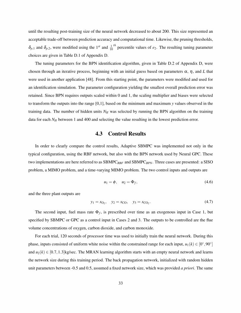
until the resulting post-training size of the neural network decreased to about 200. This size represented an
acceptable trade-off between prediction accuracy and computational time. Likewise, the pruning thresholds,
δp,1 and δp,2, were modified using the 1st and 110
th percentile values of e2. The resulting tuning parameter
choices are given in Table D.1 of Appendix D.
The tuning parameters for the BPN identification algorithm, given in Table D.2 of Appendix D, were
chosen through an iterative process, beginning with an initial guess based on parameters α , η , and L that
were used in another application [48]. From this starting point, the parameters were modified and used for
an identification simulation. The parameter configuration yielding the smallest overall prediction error was
retained. Since BPN requires outputs scaled within 0 and 1, the scaling multiplier and biases were selected
to transform the outputs into the range [0,1], based on the minimum and maximum y values observed in the
training data. The number of hidden units NH was selected by running the BPN algorithm on the training
data for each NH between 1 and 400 and selecting the value resulting in the lowest prediction error.
4.3 Control Results
In order to clearly compare the control results, Adaptive SBMPC was implemented not only in the
typical configuration, using the RBF network, but also with the BPN network used by Neural GPC. These
two implementations are here referred to as SBMPCRBF and SBMPCBPN . Three cases are presented: a SISO
problem, a MIMO problem, and a time-varying MIMO problem. The two control inputs and outputs are
u1 = φ , u2 = Φ f , (4.6)
and the three plant outputs are
y1 = xO2 , y2 = xCO, y3 = xCO2 . (4.7)
The second input, fuel mass rate Φ f , is prescribed over time as an exogenous input in Case 1, but
specified by SBMPC or GPC as a control input in Cases 2 and 3. The outputs to be controlled are the flue
volume concentrations of oxygen, carbon dioxide, and carbon monoxide.
For each trial, 120 seconds of processor time was used to initially train the neural network. During this
phase, inputs consisted of uniform white noise within the constrained range for each input, u1(k) ∈ [0◦,90◦]
and u2(k) ∈ [0.7,1.3]kg/sec. The MRAN learning algorithm starts with an empty neural network and learns
the network size during this training period. The back propagation network, initialized with random hidden
unit parameters between -0.5 and 0.5, assumed a fixed network size, which was provided a priori. The same
33
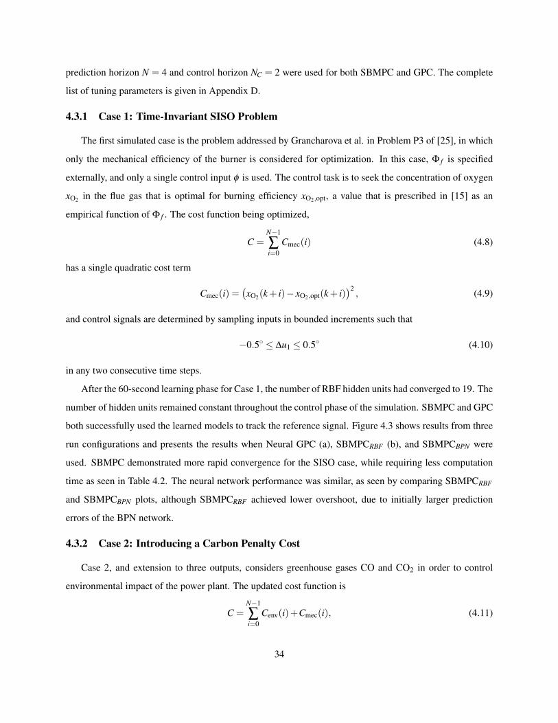
prediction horizon N = 4 and control horizon NC = 2 were used for both SBMPC and GPC. The complete
list of tuning parameters is given in Appendix D.
4.3.1 Case 1: Time-Invariant SISO Problem
The first simulated case is the problem addressed by Grancharova et al. in Problem P3 of [25], in which
only the mechanical efficiency of the burner is considered for optimization. In this case, Φ f is specified
externally, and only a single control input φ is used. The control task is to seek the concentration of oxygen
xO2 in the flue gas that is optimal for burning efficiency xO2,opt, a value that is prescribed in [15] as an
empirical function of Φ f . The cost function being optimized,
C =N−1
∑i=0
Cmec(i) (4.8)
has a single quadratic cost term
Cmec(i) =(xO2(k+ i)− xO2,opt(k+ i)
)2, (4.9)
and control signals are determined by sampling inputs in bounded increments such that
−0.5◦ ≤ ∆u1 ≤ 0.5◦ (4.10)
in any two consecutive time steps.
After the 60-second learning phase for Case 1, the number of RBF hidden units had converged to 19. The
number of hidden units remained constant throughout the control phase of the simulation. SBMPC and GPC
both successfully used the learned models to track the reference signal. Figure 4.3 shows results from three
run configurations and presents the results when Neural GPC (a), SBMPCRBF (b), and SBMPCBPN were
used. SBMPC demonstrated more rapid convergence for the SISO case, while requiring less computation
time as seen in Table 4.2. The neural network performance was similar, as seen by comparing SBMPCRBF
and SBMPCBPN plots, although SBMPCRBF achieved lower overshoot, due to initially larger prediction
errors of the BPN network.
4.3.2 Case 2: Introducing a Carbon Penalty Cost
Case 2, and extension to three outputs, considers greenhouse gases CO and CO2 in order to control
environmental impact of the power plant. The updated cost function is
C =N−1
∑i=0
Cenv(i)+Cmec(i), (4.11)
34
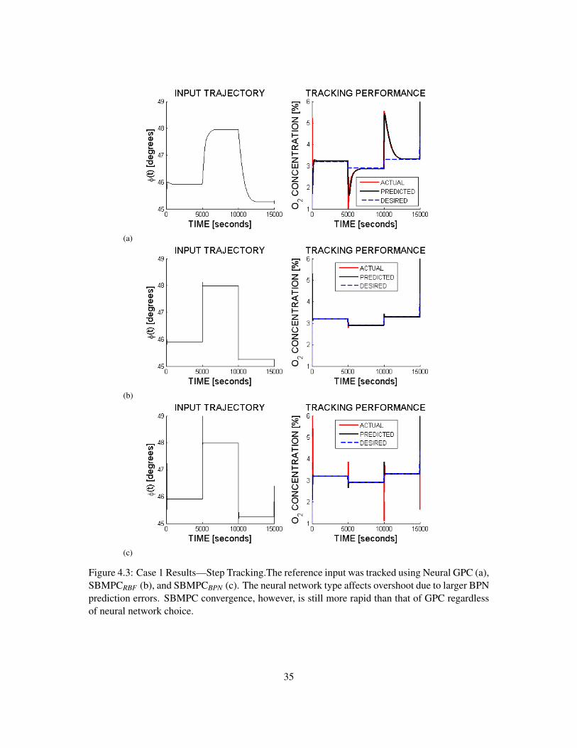
(a)
(b)
(c)
Figure 4.3: Case 1 Results—Step Tracking.The reference input was tracked using Neural GPC (a),SBMPCRBF (b), and SBMPCBPN (c). The neural network type affects overshoot due to larger BPNprediction errors. SBMPC convergence, however, is still more rapid than that of GPC regardlessof neural network choice.
35
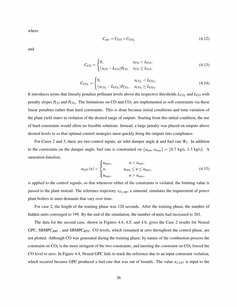
where
Cenv =CCO +CCO2 (4.12)
and
CCO =
{0, xCO < LCO,
(xCO−LCO)PCO, xCO ≥ LCO,(4.13)
CCO2 =
{0, xCO2 < LCO2 ,
(xCO2−LCO2)PCO2 , xCO2 ≥ LCO2 .(4.14)
It introduces terms that linearly penalize pollutant levels above the respective thresholds LCO2 and LCO with
penalty slopes PCO and PCO2 . The limitations on CO and CO2 are implemented as soft constraints via these
linear penalties rather than hard constraints. This is done because initial conditions and time variation of
the plant yield states in violation of the desired range of outputs. Starting from this initial condition, the use
of hard constraints would allow no feasible solutions. Instead, a large penalty was placed on outputs above
desired levels to so that optimal control strategies must quickly bring the outputs into compliance.
For Cases 2 and 3, there are two control inputs, air inlet damper angle φ and fuel rate Φ f . In addition
to the constraints on the damper angle, fuel rate is constrained on {umin,umax} = {0.7 kg/s, 1.3 kg/s}. A
saturation function,
uSAT (u) =
umax, u < umin,
u, umin ≤ u≤ umax,
umax, u > umax,
(4.15)
is applied to the control signals, so that whenever either of the constraints is violated, the limiting value is
passed to the plant instead. The reference trajectory xO2,opt, a sinusoid, simulates the requirement of power
plant boilers to meet demands that vary over time.
For case 2, the length of the training phase was 120 seconds. After the training phase, the number of
hidden units converged to 199. By the end of the simulation, the number of units had increased to 201.
The data for the second case, shown in Figures 4.4, 4.5, and 4.6, gives the Case 2 results for Neural
GPC, SBMPCRBF , and SBMPCBPN . CO levels, which remained at zero throughout the control phase, are
not plotted. Although CO was generated during the training phase, by nature of the combustion process the
constraint on CO2 is the more stringent of the two constraints, and meeting the constraint on CO2 forced the
CO level to zero. In Figure 4.4, Neural GPC fails to track the reference due to an input constraint violation,
which occured because GPC produced a fuel rate that was out of bounds. The value u2,SAT is input to the
36
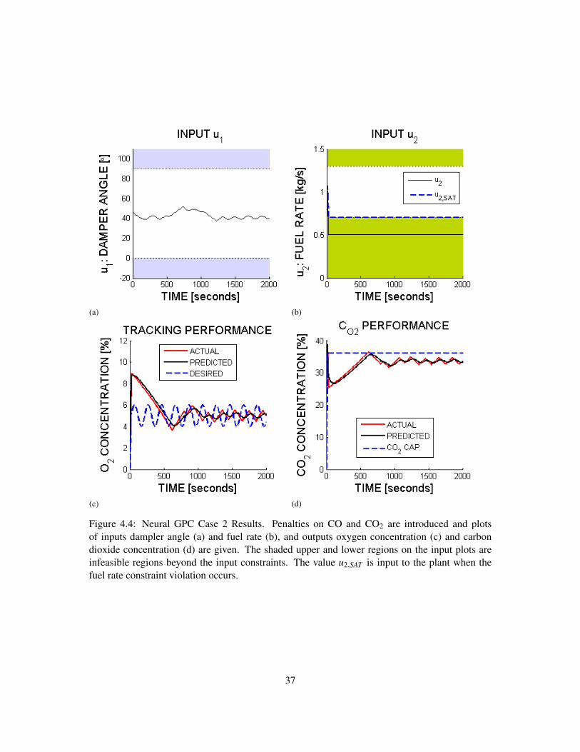
(a) (b)
(c) (d)
Figure 4.4: Neural GPC Case 2 Results. Penalties on CO and CO2 are introduced and plotsof inputs dampler angle (a) and fuel rate (b), and outputs oxygen concentration (c) and carbondioxide concentration (d) are given. The shaded upper and lower regions on the input plots areinfeasible regions beyond the input constraints. The value u2,SAT is input to the plant when thefuel rate constraint violation occurs.
37
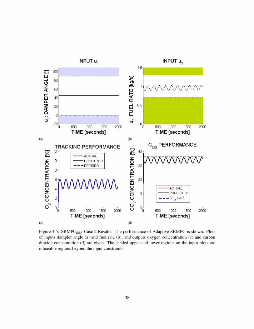
(a) (b)
(c) (d)
Figure 4.5: SBMPCRBF Case 2 Results. The performance of Adaptive SBMPC is shown. Plotsof inputs dampler angle (a) and fuel rate (b), and outputs oxygen concentration (c) and carbondioxide concentration (d) are given. The shaded upper and lower regions on the input plots areinfeasible regions beyond the input constraints.
38
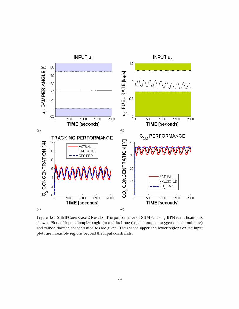
(a) (b)
(c) (d)
Figure 4.6: SBMPCBPN Case 2 Results. The performance of SBMPC using BPN identification isshown. Plots of inputs dampler angle (a) and fuel rate (b), and outputs oxygen concentration (c)and carbon dioxide concentration (d) are given. The shaded upper and lower regions on the inputplots are infeasible regions beyond the input constraints.
39

Table 4.1: Time Variation of Simulation Plant Dynamics
Time (s) Description Quantitative Changes0 to 5000 Normal boiler operation None500 to 1000 Constricted air flow Φmax is 36% smaller1000 to 1500 Damp fuel H2O added to comprise 5% of fuel mass1500 to 2000 Smaller chamber volume 15% reduction in volume
plant when the fuel rate constraint violation occurs. Because of this saturation of u2, tracking performance
is poor as u1 alone lacks the control authority to track the reference. The damper angle alone lacks the
control authority to track the reference trajectory. SBMPCRBF converges with small error and satisfaction
of output constraints. Prediction errors are rapidly corrected in the first few time steps of the control phase.
SBMPOBPN network similarly achieves overall constraint satisfaction, but the tracking is less effective due
to the prediction error of BPN. The execution time of SBMPORBF was improved over that of SBMPOBPN ,
as seen in Table 4.2, which is primarily due to the smaller number of graph node expansions required when
model predictions are more accurate. This time is also directly proportional to number of hidden units
required to represent the system. The MRAN algorithm converged to 201 hidden units, whereas the fixed
number of hidden units for the BPN network was 39.
4.3.3 Case 3: Control System Adaptation Under Changing Dynamics
The third simulation case demonstrates the versatility of the adaptive algorithms as changes in plant
dynamics are introduced that require active model updates. The online identification algorithms are able to
quickly adjust to changing plant behavior, either by back-propagation (BPN) or the EKF optimization of
MRAN (RBF).
In the simulation, plant dynamics are applied as step parameter changes at the beginning of each 500
second interval of simulation time. The nature of the changing boiler dynamics is presented in Table 4.1.
Each change is from the normal dynamic behavior, such that the changes mentioned are in effect during the
interval but revert back to the normal values.
For case 3, the length to the training phase was 120 seconds. After the training phase, the number of
hidden units converged to 199. By the end of the simulation, the number of units had increased to 205.
The data for the third case, shown in Figures 4.7, 4.8, and 4.9, indicates that after each shift in plant
dynamics, the neural networks are adapted and prediction errors were corrected. In Figure 4.7, Neural
GPC exhibited significant and sustained tracking error due to the u2 input constraint violation that was
40
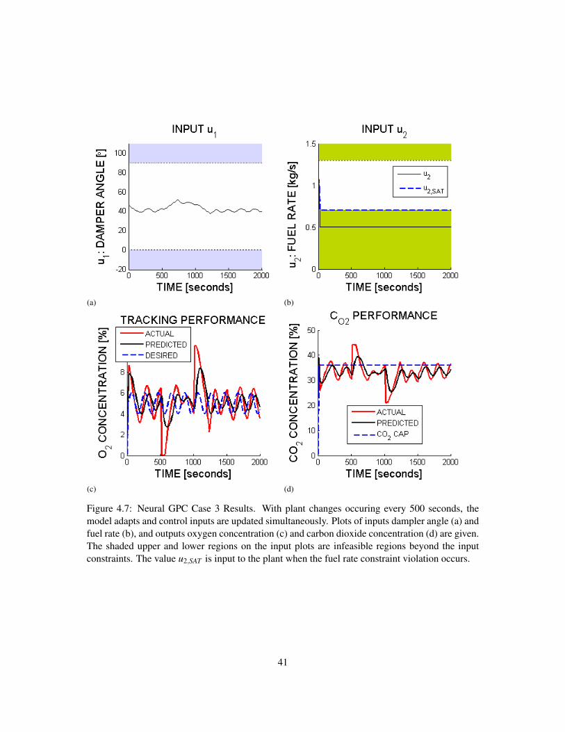
(a) (b)
(c) (d)
Figure 4.7: Neural GPC Case 3 Results. With plant changes occuring every 500 seconds, themodel adapts and control inputs are updated simultaneously. Plots of inputs dampler angle (a) andfuel rate (b), and outputs oxygen concentration (c) and carbon dioxide concentration (d) are given.The shaded upper and lower regions on the input plots are infeasible regions beyond the inputconstraints. The value u2,SAT is input to the plant when the fuel rate constraint violation occurs.
41
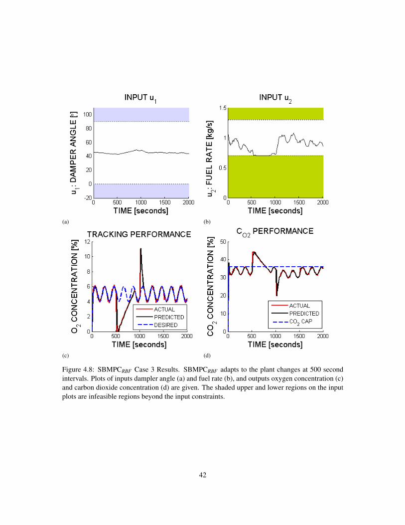
(a) (b)
(c) (d)
Figure 4.8: SBMPCRBF Case 3 Results. SBMPCRBF adapts to the plant changes at 500 secondintervals. Plots of inputs dampler angle (a) and fuel rate (b), and outputs oxygen concentration (c)and carbon dioxide concentration (d) are given. The shaded upper and lower regions on the inputplots are infeasible regions beyond the input constraints.
42

(a) (b)
(c) (d)
Figure 4.9: SBMPCBPN Case 3 Results. SBMPCBPN adapts to the plant changes at 500 secondintervals. Plots of inputs dampler angle (a) and fuel rate (b), and outputs oxygen concentration (c)and carbon dioxide concentration (d) are given. The shaded upper and lower regions on the inputplots are infeasible regions beyond the input constraints.
43
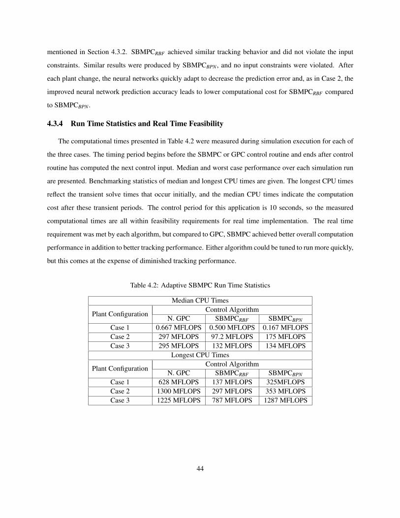
mentioned in Section 4.3.2. SBMPCRBF achieved similar tracking behavior and did not violate the input
constraints. Similar results were produced by SBMPCBPN , and no input constraints were violated. After
each plant change, the neural networks quickly adapt to decrease the prediction error and, as in Case 2, the
improved neural network prediction accuracy leads to lower computational cost for SBMPCRBF compared
to SBMPCBPN .
4.3.4 Run Time Statistics and Real Time Feasibility
The computational times presented in Table 4.2 were measured during simulation execution for each of
the three cases. The timing period begins before the SBMPC or GPC control routine and ends after control
routine has computed the next control input. Median and worst case performance over each simulation run
are presented. Benchmarking statistics of median and longest CPU times are given. The longest CPU times
reflect the transient solve times that occur initially, and the median CPU times indicate the computation
cost after these transient periods. The control period for this application is 10 seconds, so the measured
computational times are all within feasibility requirements for real time implementation. The real time
requirement was met by each algorithm, but compared to GPC, SBMPC achieved better overall computation
performance in addition to better tracking performance. Either algorithm could be tuned to run more quickly,
but this comes at the expense of diminished tracking performance.
Table 4.2: Adaptive SBMPC Run Time Statistics
Median CPU Times
Plant ConfigurationControl Algorithm
N. GPC SBMPCRBF SBMPCBPN
Case 1 0.667 MFLOPS 0.500 MFLOPS 0.167 MFLOPSCase 2 297 MFLOPS 97.2 MFLOPS 175 MFLOPSCase 3 295 MFLOPS 132 MFLOPS 134 MFLOPS
Longest CPU Times
Plant ConfigurationControl Algorithm
N. GPC SBMPCRBF SBMPCBPN
Case 1 628 MFLOPS 137 MFLOPS 325MFLOPSCase 2 1300 MFLOPS 297 MFLOPS 353 MFLOPSCase 3 1225 MFLOPS 787 MFLOPS 1287 MFLOPS
44
4.3.5 Tuning the Control Algorithms
Compared with the neural network algorithms, the NMPC algorithms involved less effort to tune. For
both SBMPC and GPC the prediction horizon N = 4 was chosen large enough to limit the overshoot of the
transient behavior of the controlled system. For both algorithms the control horizon NC = 2 was chosen to
keep the computations small.
After these were fixed, the only remaining SBMPC tuning parameter is the branchout factor B. This
parameter allows a trade-off between low computational cost (small B) and low tracking error (large B). The
value B = 60 was selected after trial simulations with various values.
In order to tune the Newton solver of GPC, a solver tolerance ε , iteration limit Imax, input constraint
sharpness s, and damping factor λ were selected. The parameters ε and Imax allow for a trade-off between
computational cost and tracking error, so they were selected to match the Case 1 steady state tracking error
performance of SBMPC. The parameters s and λ , if not properly selected, led to instability of GPC. The
damping factor was selected based on trial and error, which was a tedious process because this search
spanned many orders of magnitude before producing stable results. The value of s = 10−12 suggested in
[67] produced stable solver results. Smaller values also produced stable results, while larger values led to
instability. Even though the solver results were stable in the sense that the Newton solver converged to finite
values, no tuning configuration was found that avoided an input constraint violation under the conditions of
Cases 2 and 3.
4.4 Summary
Adaptive SBMPC, an adaptive approach to nonlinear model predictive control, is presented and applied
in simulation to a combustion control problem from literature. For comparison, the nonlinear dynamics of
coal combustion within a commercial boiler were learned and controlled using Neural GPC as well as Adap-
tive SBMPC. SBMPO was demonstrated as an efficient nonlinear optimization was performed and close
reference tracking was achieved. Strengths of SBMPO, including computational speed, ease of tuning, and
compatability with any model, were demonstrated in a MIMO nonlinear application. A direct comparison of
the RBF and BPN neural network identification approaches is given using SBMPO optimization with each
neural network type. The major strengths of the RBF network are the ability to modify the neural network
structure during controller operation and the ability to learn plant behavior without the a priori specification
of network size.
45
The original problem was extended to consider additional outputs and an additional control input as
well as time-varying plant dynamics. Adaptive SBMPC was shown to be capable of rapid adjustments to
changes in plant behavior and efficient nonlinear optimization for MIMO systems. The achieved execution
times were, in the worst case, well under the ten-second sampling interval appropriate for feedback control
of combustion.
For the purpose of comparison, results were presented for a combustion system identification and con-
trol problem. The MIMO system was identified using BPN and RBF neural networks and the Adaptive
SBMPC and Neural GPC control systems were used to perform NMPC. The results presented in Case 3
are the first control results of a time-varying MIMO plant using Neural GPC as well as the first control
results for SBMPC implemented with the BPN neural network model. The results indicate that both neural
network structures are capable of representing the nonlinear system and both control methodologies easily
handle the SISO control case. When the MIMO problem was considered, Neural GPC tended to violate the
input constraints, which led to poor reference tracking. By design, Adaptive SBMPC cannot violate input
constraints and good tracking results were achieved using both the RBF and BPN neural network structures.
Adaptive SBMPC generally achieved better computational times and in the worst case did not exceed the
control period of 10 seconds.
One potential improvement to Adaptive SBMPC, the learning of A∗ search heuristics for general non-
linear systems, which would enable further computational improvements, are planned as future work. This
improved implementation will exploit past optimization cost information to speed up subsequent optimiza-
tions for the same plant. Further computational improvement is possible using parallel computations. During
SBMPO execution, the majority of the the computational effort is spent on expansion of nodes. These expan-
sions may be computed in parallel in order to leverage the capabilities of multi-core CPU or GPU hardware.
These computation improvements will allow the application of Adaptive SBMPC to larger systems as well
as systems with fast real-time computation requirements.
46
CHAPTER 5
APPLICATION TO FLOW SEPARATION CONTROL
5.1 Introduction
For decades, flow separation has been of particular interest in engineering applications for which im-
proved aerodynamic performance is desired. Control of flow separation, both active and passive, is a key
component of existing aviation technology. Passive control methods, such as leading edge surface rough-
ness or the inclusion of vortex generators, rely on stationary structural components to produce a reduction or
delay in separation effects. These techniques typically produce an early transition to turbulence or stream-
wise vortical structures, each of which has been shown to mitigate separation [40]. The effectiveness of
passive techniques is limited in comparison with active techniques, which rely on powered mechanisms to
alter the flow, especially when conditions different from the design point are considered [10]. These types
of off-design conditions are common for aeronautical systems that are deployed in diverse environments,
including micro-aerial vehicles and full-size aircraft that perform maneuvers.
The significant increase in capability and decrease in cost of computing hardware has led to the fea-
sibility of active control techniques of increasing sophistication. Both open-loop and closed-loop control
schemes have been applied to flow control problems and there is evidence that closed loop approaches offer
significant improvement in performance over open-loop control [55][34].
Several areas of flow control research, including suppression of cavity flow resonant tones and mitigation
of flow separation, have advanced rapidly in recent years as new technologies have both created demand
for and expanded the capabilities of such systems. The study of cavity flow control has demonstrated
that mathematical techniques such as Proper Orthogonal Decomposition (POD) and model reduction are
effective tools for controlling aerodynamic systems [50][20] under limited Reynolds number conditions and
a fixed angle of attack. While these studies incorporated flow visualization and analysis efforts to produce
nonlinear models that are effective for developing open-loop control strategies, it has been more practical
to linearize these models for the sake of computational efficiency when implementing real-time closed loop
control [55][34].
47
Frequency domain methods have been applied to model and control the flow dynamics in flow control
and related applications [49][12][42]. Nonlinear POD methods similar to those applied to cavity flow have
also been used for flow separation [22]; however, these models exhibit little robustness and have only been
used to perform open-loop control. Actuator development has also been key to the recent advances in the
field of flow separation control. Both synthetic jet unsteady actuators [71][70] and steady microjet actuators
[12][4] have been effective in closed-loop separation control experiments. Because of the advantage of
high momentum capability with low power requirements [41], microjet arrays are used as actuators in this
research. These actuators are capable of both pulsed and steady blowing.
Nonlinear model predictive control (NMPC) has been proposed for flow control, but “a huge numerical
burden” is listed as a drawback of such methods [54]. The method presented in this dissertation, Adaptive
Sampling Based Model Predictive Control (Adaptive SBMPC) [64], is a new paradigm for NMPC that
is computationally efficient. Adaptive SBMPC differs from past adaptive, closed-loop approaches to flow
control by identifying a nonlinear model for control. This chapter provides the experimental results, Particle
Image Velocimetry (PIV) visualization, and detailed analysis of the flow separation control problem. The
identification and control processing is executed in real time, demonstrating the potential of this method for
in-flight application.
5.1.1 Control Objective
The primary objective of this research is to maximize the lift coefficient CL by means of delaying the
onset of separation as well as controlling flows with initially-separated boundary layers. The experimental
model is not instrumented with sensors capable of approximating the drag coefficient CD, but the lift-drag
ratio CL/CD is typically also improved when flow separation is mitigated and CL increases. Given a discrete
time series of multiple sensor measurements located along an airfoil’s chord (inputs), the proposed research
aims to determine an optimal series of microjet pressure signals (outputs), maximizing the lift performance
of the airfoil. The control system should achieve this task for a broad range of steady or dynamically-
prescribed Reynolds numbers or angle of attack parameters. This is to be accomplished without direct
measurement of either parameter and without the modification of tuning parameters.
48

Figure 5.1: Sampling Based Model Predictive Control Summary. The algorithm discretizes theinput space and makes model-based state predictions, xk+ j, in order to minimize a cost function.
5.2 Control Method
As a means of solving Model Predictive Optimization problems without computing gradients, Sampling
Based Model Predictive Optimization (SBMPO) has been developed and implemented on both simulated
and experimental platforms [64][63][19][18][1]. One key advantage of SBMPO is the ability to find globally
optimal solutions, while other methods that rely on linearization are likely to converge to locally minimum
solutions. A second advantage, computational efficiency enables the use of SBMPO to solve real time
NMPC trajectories. When SBMPO is combined with a neural network model of system behavior, the
overall method for identification and control is called Adaptive Sampling Based Model Predictive Control
(Adaptive SBMPC). SBMPO may be applied to solve the nonlinear optimization problem,
min{u(k),...,u(k+N−1)}
N−1
∑i=0
C (y(k+ i+1)− r(k+ i+1)) , (5.1)
subject to the nonlinear state space equations,
x(k+ i) = g(x(k+ i−1),u(k+ i−1)), (5.2)
y(k) = h(x(k)), (5.3)
and the constraints,
x(k+ i) ∈ X f ree ∀ i≤ N, (5.4)
u(k+ i) ∈ U f ree ∀ i≤ N, (5.5)
49
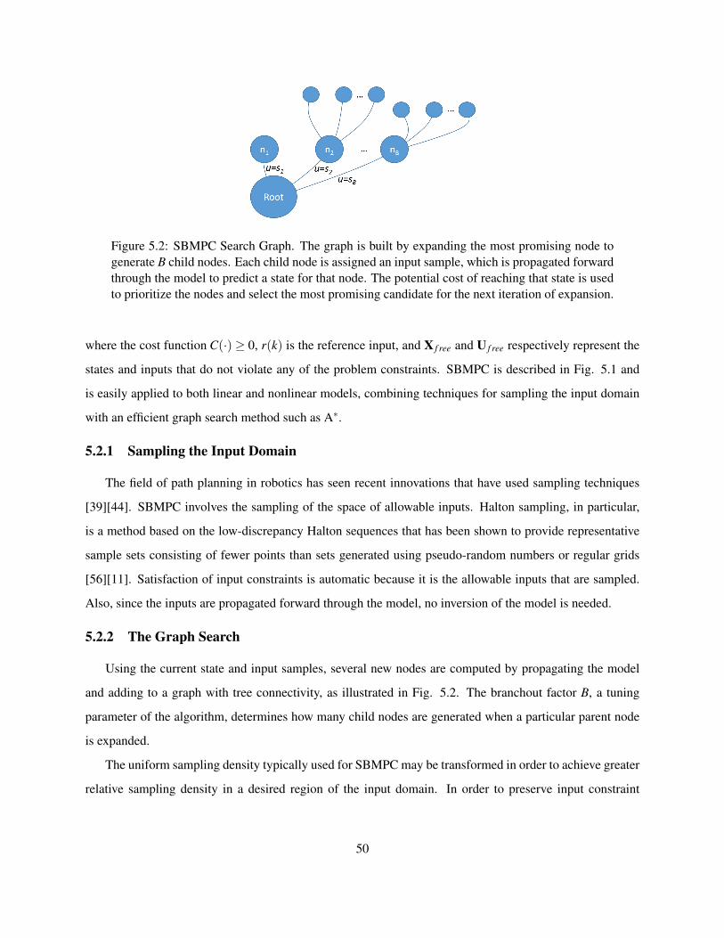
Figure 5.2: SBMPC Search Graph. The graph is built by expanding the most promising node togenerate B child nodes. Each child node is assigned an input sample, which is propagated forwardthrough the model to predict a state for that node. The potential cost of reaching that state is usedto prioritize the nodes and select the most promising candidate for the next iteration of expansion.
where the cost function C(·)≥ 0, r(k) is the reference input, and X f ree and U f ree respectively represent the
states and inputs that do not violate any of the problem constraints. SBMPC is described in Fig. 5.1 and
is easily applied to both linear and nonlinear models, combining techniques for sampling the input domain
with an efficient graph search method such as A∗.
5.2.1 Sampling the Input Domain
The field of path planning in robotics has seen recent innovations that have used sampling techniques
[39][44]. SBMPC involves the sampling of the space of allowable inputs. Halton sampling, in particular,
is a method based on the low-discrepancy Halton sequences that has been shown to provide representative
sample sets consisting of fewer points than sets generated using pseudo-random numbers or regular grids
[56][11]. Satisfaction of input constraints is automatic because it is the allowable inputs that are sampled.
Also, since the inputs are propagated forward through the model, no inversion of the model is needed.
5.2.2 The Graph Search
Using the current state and input samples, several new nodes are computed by propagating the model
and adding to a graph with tree connectivity, as illustrated in Fig. 5.2. The branchout factor B, a tuning
parameter of the algorithm, determines how many child nodes are generated when a particular parent node
is expanded.
The uniform sampling density typically used for SBMPC may be transformed in order to achieve greater
relative sampling density in a desired region of the input domain. In order to preserve input constraint
50
satisfaction, the transformation must guarantee that no valid inputs are mapped to invalid inputs. Using a
nonuniform sampling density can improve the performance of SBMPC by sampling large input changes
more coarsely while sampling small input changes more finely. This finer sampling allows the trajectory to
converge with small steady-state errors.
The Halton sequence algorithm, which is potentially used thousands of times at each time interval when
the SBMPC routine is called, was a major contributor to the total runtime of SBMPC. During benchmark
testing of C code on multiple machines, batches of 1 million elements of a Halton sequence were computed,
and then precomputed batches of equivalent size were loaded from a binary file. The median CPU time
required to compute the samples was 210 milliseconds, while the median time required to load the precom-
puted values was 1 millisecond; therefore, computing these samples offline and storing them in a binary file
enables the run-time code to execute much faster while yielding identical results. The offline computation
of these Halton samples is a contribution of this dissertation and reduces the run-time computational cost of
SBMPC.
5.2.3 Nonlinear Modelling
Previous adaptive flow separation research has aimed to capture the nonlinear dynamics of the flow
field by identifying an instantaneously linearized model that varies with time. The optimization of a linear
model has the advantages of speed and simplicity over those that consider nonlinear models. The unmodeled
dynamics, however, can cause such techniques to be suboptimal and even unstable.
Nonlinear POD Methods. Proper Orthogonal Decomposition (POD) techniques have been used to
identify models in the form of polynomial difference equations [65][36] that are sufficient for open loop
control design [50]. However, due to computational expense, closed loop flow control implementations
have been limited to linear models [54]. Although SBMPO has the ability to optimize inputs to a POD
model, POD models are steady state in nature and do not capture the transient behavior or hysteresis effects
that are necessary to control dynamic stall.
SBMPO Compatibility with More General Models. A primary advantage of SBMPO over alterna-
tive optimization methods is that this technique has no intrinsic preference for linear models over nonlinear
models, and the algorithm does not need to compute closed-form gradients. This allows SBMPO to be
applied to a more general class of systems than could be handled by previous methods. Even systems with
strong nonlinearities or non-differentiable functions can be optimized using SBMPO.
51
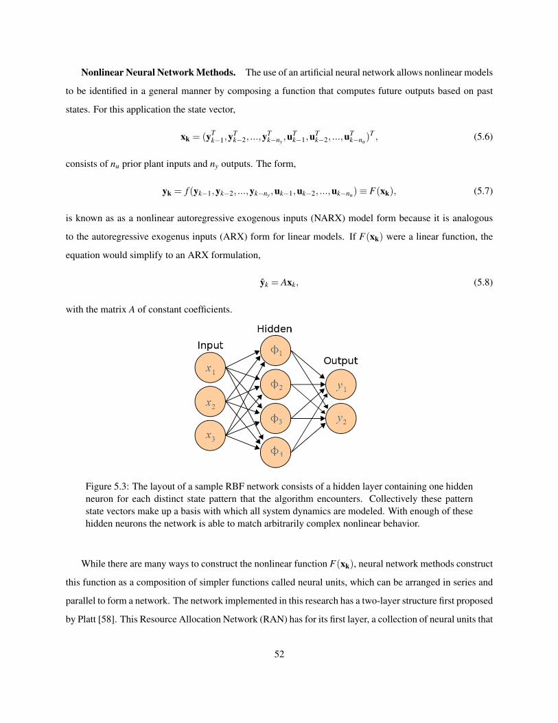
Nonlinear Neural Network Methods. The use of an artificial neural network allows nonlinear models
to be identified in a general manner by composing a function that computes future outputs based on past
states. For this application the state vector,
xk = (yTk−1,y
Tk−2, ...,y
Tk−ny
,uTk−1,u
Tk−2, ...,u
Tk−nu
)T , (5.6)
consists of nu prior plant inputs and ny outputs. The form,
yk = f (yk−1,yk−2, ...,yk−ny ,uk−1,uk−2, ...,uk−nu)≡ F(xk), (5.7)
is known as as a nonlinear autoregressive exogenous inputs (NARX) model form because it is analogous
to the autoregressive exogenus inputs (ARX) form for linear models. If F(xk) were a linear function, the
equation would simplify to an ARX formulation,
yk = Axk, (5.8)
with the matrix A of constant coefficients.
Figure 5.3: The layout of a sample RBF network consists of a hidden layer containing one hiddenneuron for each distinct state pattern that the algorithm encounters. Collectively these patternstate vectors make up a basis with which all system dynamics are modeled. With enough of thesehidden neurons the network is able to match arbitrarily complex nonlinear behavior.
While there are many ways to construct the nonlinear function F(xk), neural network methods construct
this function as a composition of simpler functions called neural units, which can be arranged in series and
parallel to form a network. The network implemented in this research has a two-layer structure first proposed
by Platt [58]. This Resource Allocation Network (RAN) has for its first layer, a collection of neural units that
52
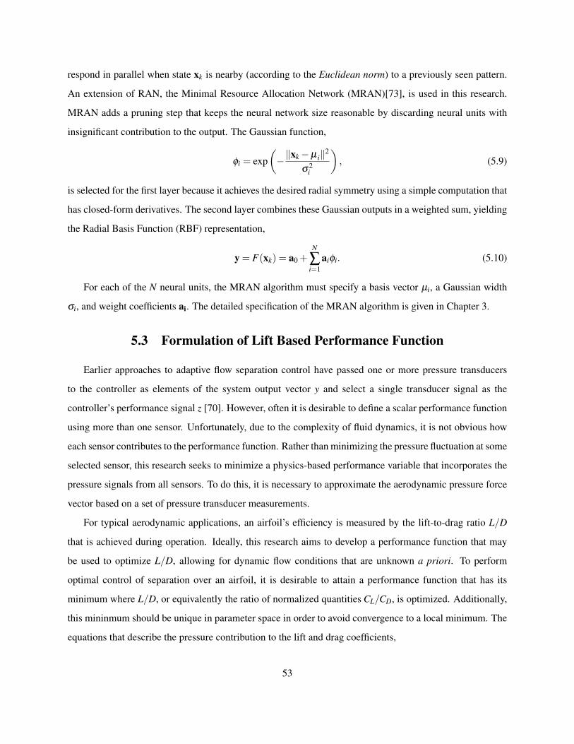
respond in parallel when state xk is nearby (according to the Euclidean norm) to a previously seen pattern.
An extension of RAN, the Minimal Resource Allocation Network (MRAN)[73], is used in this research.
MRAN adds a pruning step that keeps the neural network size reasonable by discarding neural units with
insignificant contribution to the output. The Gaussian function,
φi = exp(−‖xk−µ i‖2
σ2i
), (5.9)
is selected for the first layer because it achieves the desired radial symmetry using a simple computation that
has closed-form derivatives. The second layer combines these Gaussian outputs in a weighted sum, yielding
the Radial Basis Function (RBF) representation,
y = F(xk) = a0 +N
∑i=1
aiφi. (5.10)
For each of the N neural units, the MRAN algorithm must specify a basis vector µi, a Gaussian width
σi, and weight coefficients ai. The detailed specification of the MRAN algorithm is given in Chapter 3.
5.3 Formulation of Lift Based Performance Function
Earlier approaches to adaptive flow separation control have passed one or more pressure transducers
to the controller as elements of the system output vector y and select a single transducer signal as the
controller’s performance signal z [70]. However, often it is desirable to define a scalar performance function
using more than one sensor. Unfortunately, due to the complexity of fluid dynamics, it is not obvious how
each sensor contributes to the performance function. Rather than minimizing the pressure fluctuation at some
selected sensor, this research seeks to minimize a physics-based performance variable that incorporates the
pressure signals from all sensors. To do this, it is necessary to approximate the aerodynamic pressure force
vector based on a set of pressure transducer measurements.
For typical aerodynamic applications, an airfoil’s efficiency is measured by the lift-to-drag ratio L/D
that is achieved during operation. Ideally, this research aims to develop a performance function that may
be used to optimize L/D, allowing for dynamic flow conditions that are unknown a priori. To perform
optimal control of separation over an airfoil, it is desirable to attain a performance function that has its
minimum where L/D, or equivalently the ratio of normalized quantities CL/CD, is optimized. Additionally,
this mininmum should be unique in parameter space in order to avoid convergence to a local minimum. The
equations that describe the pressure contribution to the lift and drag coefficients,
53
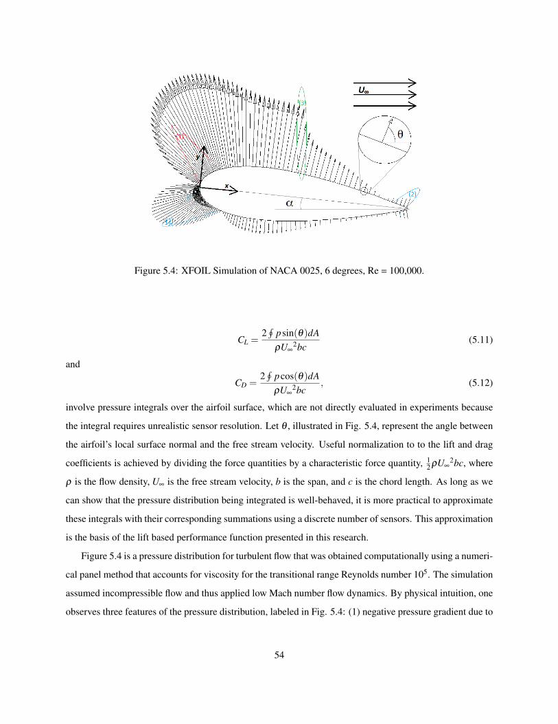
Figure 5.4: XFOIL Simulation of NACA 0025, 6 degrees, Re = 100,000.
CL =2∮
psin(θ)dAρU∞
2bc(5.11)
and
CD =2∮
pcos(θ)dAρU∞
2bc, (5.12)
involve pressure integrals over the airfoil surface, which are not directly evaluated in experiments because
the integral requires unrealistic sensor resolution. Let θ , illustrated in Fig. 5.4, represent the angle between
the airfoil’s local surface normal and the free stream velocity. Useful normalization to to the lift and drag
coefficients is achieved by dividing the force quantities by a characteristic force quantity, 12 ρU∞
2bc, where
ρ is the flow density, U∞ is the free stream velocity, b is the span, and c is the chord length. As long as we
can show that the pressure distribution being integrated is well-behaved, it is more practical to approximate
these integrals with their corresponding summations using a discrete number of sensors. This approximation
is the basis of the lift based performance function presented in this research.
Figure 5.4 is a pressure distribution for turbulent flow that was obtained computationally using a numeri-
cal panel method that accounts for viscosity for the transitional range Reynolds number 105. The simulation
assumed incompressible flow and thus applied low Mach number flow dynamics. By physical intuition, one
observes three features of the pressure distribution, labeled in Fig. 5.4: (1) negative pressure gradient due to
54
Figure 5.5: Airfoil Microjet Array and Pressure Transducer Schematic.
the acceleration caused by the impeded flow, (2) locally maximum positive pressure locations correspond-
ing to the two stagnation points (fore and aft), and (3) apparent discontinuity on the top surface, indicating
early stages of flow separation at the rear of the airfoil. Inspecting this and many other pressure distribution
plots has led to some key observations. First, the surface pressure will never exceed the free stream stag-
nation pressure; this bounds the pressure distribution from above. Additionally, the surface pressure will
be bounded from below by the solution of the potential flow (inviscid case, Re→ ∞), which can be solved
analytically by using a conformal mapping. Lastly, the gradient ∂ p∂x is bounded as long as we consider in-
compressible Mach numbers (no shocks). Furthermore, the separation point and the high turning angles at
the leading edge produce the largest gradients along the chord.
As a result of these observations, it is hypothesized that a limited number of discrete pressure measure-
ments can be used to compute an approximation of aerodynamic forces that is sufficiently accurate to use as
a control feedback variable. The aerodynamic pressure force is by definition a path integral of the pressure
normal vectors around the surface of the airfoil. As described in Eqs. (5.11) and (5.12), this vector can be
decomposed into two components: lift, which is normal to the free stream, and drag, which is parallel to
the free stream. Note that this is only one of the components comprising the total drag force since shear
force must also be accounted for. It is assumed that pressure data alone will provide a sufficient estimation
for separation control purposes. This assumption is justified by the data presented in Appendix E, which
indicates that points of maximal lift and points of maximal L/D are coincident for transitional Reynolds
numbers.
An approximation of lift that is suitable for control purposes must practically preserve the global maxi-
mum of the actual lift quantity. The design of Fig. 5.14 is based on the hypothesis that four pressure sensors
55
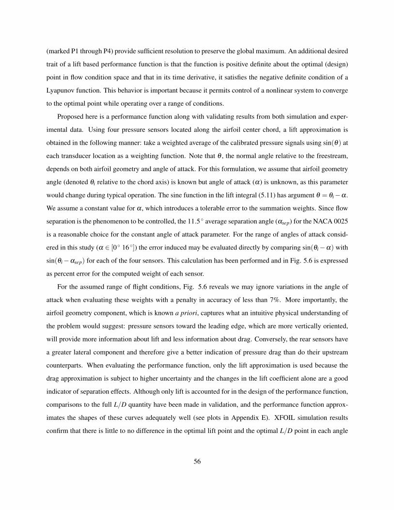
(marked P1 through P4) provide sufficient resolution to preserve the global maximum. An additional desired
trait of a lift based performance function is that the function is positive definite about the optimal (design)
point in flow condition space and that in its time derivative, it satisfies the negative definite condition of a
Lyapunov function. This behavior is important because it permits control of a nonlinear system to converge
to the optimal point while operating over a range of conditions.
Proposed here is a performance function along with validating results from both simulation and exper-
imental data. Using four pressure sensors located along the airfoil center chord, a lift approximation is
obtained in the following manner: take a weighted average of the calibrated pressure signals using sin(θ) at
each transducer location as a weighting function. Note that θ , the normal angle relative to the freestream,
depends on both airfoil geometry and angle of attack. For this formulation, we assume that airfoil geometry
angle (denoted θi relative to the chord axis) is known but angle of attack (α) is unknown, as this parameter
would change during typical operation. The sine function in the lift integral (5.11) has argument θ = θi−α .
We assume a constant value for α , which introduces a tolerable error to the summation weights. Since flow
separation is the phenomenon to be controlled, the 11.5 ◦ average separation angle (αsep) for the NACA 0025
is a reasonable choice for the constant angle of attack parameter. For the range of angles of attack consid-
ered in this study (α ∈ [0 ◦ 16 ◦]) the error induced may be evaluated directly by comparing sin(θi−α) with
sin(θi−αsep) for each of the four sensors. This calculation has been performed and in Fig. 5.6 is expressed
as percent error for the computed weight of each sensor.
For the assumed range of flight conditions, Fig. 5.6 reveals we may ignore variations in the angle of
attack when evaluating these weights with a penalty in accuracy of less than 7%. More importantly, the
airfoil geometry component, which is known a priori, captures what an intuitive physical understanding of
the problem would suggest: pressure sensors toward the leading edge, which are more vertically oriented,
will provide more information about lift and less information about drag. Conversely, the rear sensors have
a greater lateral component and therefore give a better indication of pressure drag than do their upstream
counterparts. When evaluating the performance function, only the lift approximation is used because the
drag approximation is subject to higher uncertainty and the changes in the lift coefficient alone are a good
indicator of separation effects. Although only lift is accounted for in the design of the performance function,
comparisons to the full L/D quantity have been made in validation, and the performance function approx-
imates the shapes of these curves adequately well (see plots in Appendix E). XFOIL simulation results
confirm that there is little to no difference in the optimal lift point and the optimal L/D point in each angle
56
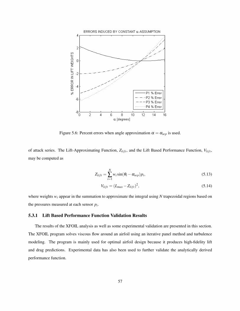
Figure 5.6: Percent errors when angle approximation α = αsep is used.
of attack series. The Lift-Approximating Function, Zli f t , and the Lift Based Performance Function, Vli f t ,
may be computed as
Zli f t =N
∑i=1
wi sin(θi−αsep)pi, (5.13)
Vli f t = (Lmax−Zli f t)2, (5.14)
where weights wi appear in the summation to approximate the integral using N trapezoidal regions based on
the pressures measured at each sensor pi.
5.3.1 Lift Based Performance Function Validation Results
The results of the XFOIL analysis as well as some experimental validation are presented in this section.
The XFOIL program solves viscous flow around an airfoil using an iterative panel method and turbulence
modeling. The program is mainly used for optimal airfoil design because it produces high-fidelity lift
and drag predictions. Experimental data has also been used to further validate the analytically derived
performance function.
57
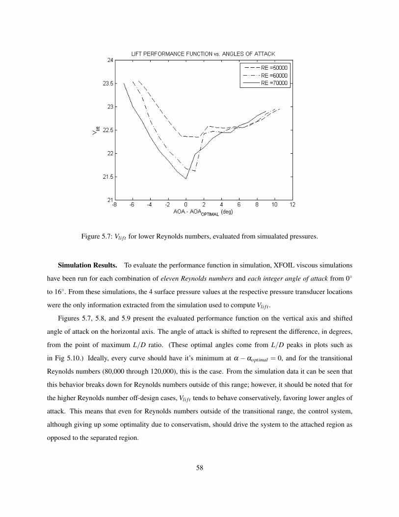
Figure 5.7: Vli f t for lower Reynolds numbers, evaluated from simualated pressures.
Simulation Results. To evaluate the performance function in simulation, XFOIL viscous simulations
have been run for each combination of eleven Reynolds numbers and each integer angle of attack from 0◦
to 16◦. From these simulations, the 4 surface pressure values at the respective pressure transducer locations
were the only information extracted from the simulation used to compute Vli f t .
Figures 5.7, 5.8, and 5.9 present the evaluated performance function on the vertical axis and shifted
angle of attack on the horizontal axis. The angle of attack is shifted to represent the difference, in degrees,
from the point of maximum L/D ratio. (These optimal angles come from L/D peaks in plots such as
in Fig 5.10.) Ideally, every curve should have it’s minimum at α −αoptimal = 0, and for the transitional
Reynolds numbers (80,000 through 120,000), this is the case. From the simulation data it can be seen that
this behavior breaks down for Reynolds numbers outside of this range; however, it should be noted that for
the higher Reynolds number off-design cases, Vli f t tends to behave conservatively, favoring lower angles of
attack. This means that even for Reynolds numbers outside of the transitional range, the control system,
although giving up some optimality due to conservatism, should drive the system to the attached region as
opposed to the separated region.
58
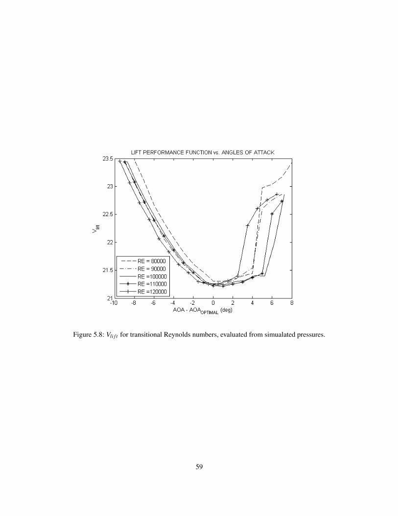
Figure 5.8: Vli f t for transitional Reynolds numbers, evaluated from simualated pressures.
59
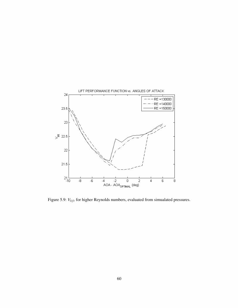
Figure 5.9: Vli f t for higher Reynolds numbers, evaluated from simualated pressures.
60
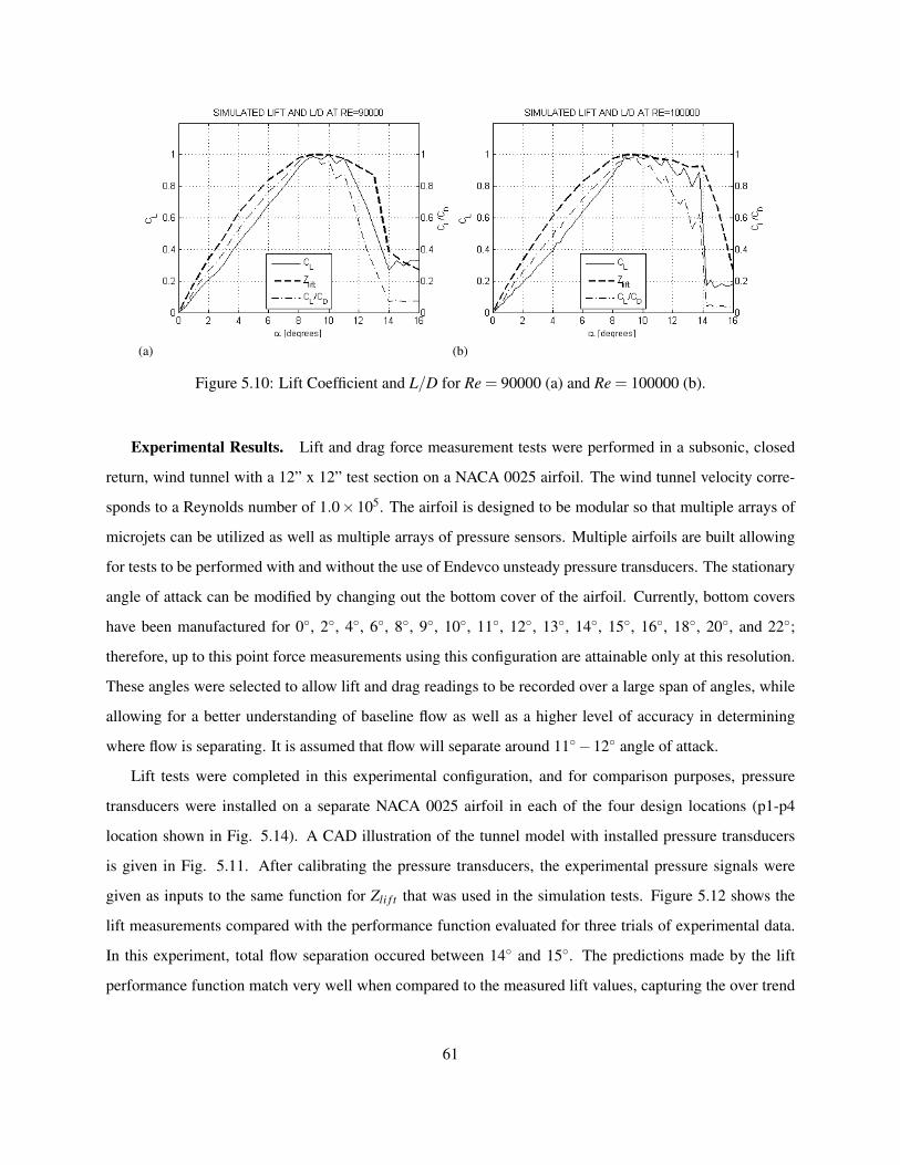
(a) (b)
Figure 5.10: Lift Coefficient and L/D for Re = 90000 (a) and Re = 100000 (b).
Experimental Results. Lift and drag force measurement tests were performed in a subsonic, closed
return, wind tunnel with a 12” x 12” test section on a NACA 0025 airfoil. The wind tunnel velocity corre-
sponds to a Reynolds number of 1.0×10⁵. The airfoil is designed to be modular so that multiple arrays of
microjets can be utilized as well as multiple arrays of pressure sensors. Multiple airfoils are built allowing
for tests to be performed with and without the use of Endevco unsteady pressure transducers. The stationary
angle of attack can be modified by changing out the bottom cover of the airfoil. Currently, bottom covers
have been manufactured for 0◦, 2◦, 4◦, 6◦, 8◦, 9◦, 10◦, 11◦, 12◦, 13◦, 14◦, 15◦, 16◦, 18◦, 20◦, and 22◦;
therefore, up to this point force measurements using this configuration are attainable only at this resolution.
These angles were selected to allow lift and drag readings to be recorded over a large span of angles, while
allowing for a better understanding of baseline flow as well as a higher level of accuracy in determining
where flow is separating. It is assumed that flow will separate around 11◦−12◦ angle of attack.
Lift tests were completed in this experimental configuration, and for comparison purposes, pressure
transducers were installed on a separate NACA 0025 airfoil in each of the four design locations (p1-p4
location shown in Fig. 5.14). A CAD illustration of the tunnel model with installed pressure transducers
is given in Fig. 5.11. After calibrating the pressure transducers, the experimental pressure signals were
given as inputs to the same function for Zli f t that was used in the simulation tests. Figure 5.12 shows the
lift measurements compared with the performance function evaluated for three trials of experimental data.
In this experiment, total flow separation occured between 14◦ and 15◦. The predictions made by the lift
performance function match very well when compared to the measured lift values, capturing the over trend
61
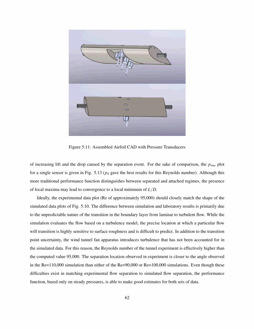
Figure 5.11: Assembled Airfoil CAD with Pressure Transducers
of increasing lift and the drop caused by the separation event. For the sake of comparison, the prms plot
for a single sensor is given in Fig. 5.13 (p4 gave the best results for this Reynolds number). Although this
more traditional performance function distinguishes between separated and attached regimes, the presence
of local maxima may lead to convergence to a local minimum of L/D.
Ideally, the experimental data plot (Re of approximately 95,000) should closely match the shape of the
simulated data plots of Fig. 5.10. The difference between simulation and laboratory results is primarily due
to the unpredictable nature of the transition in the boundary layer from laminar to turbulent flow. While the
simulation evaluates the flow based on a turbulence model, the precise location at which a particular flow
will transition is highly sensitive to surface roughness and is difficult to predict. In addition to the transition
point uncertainty, the wind tunnel fan apparatus introduces turbulence that has not been accounted for in
the simulated data. For this reason, the Reynolds number of the tunnel experiment is effectively higher than
the computed value 95,000. The separation location observed in experiment is closer to the angle observed
in the Re=110,000 simulation than either of the Re=90,000 or Re=100,000 simulations. Even though these
difficulties exist in matching experimental flow separation to simulated flow separation, the performance
function, based only on steady pressures, is able to make good estimates for both sets of data.
62
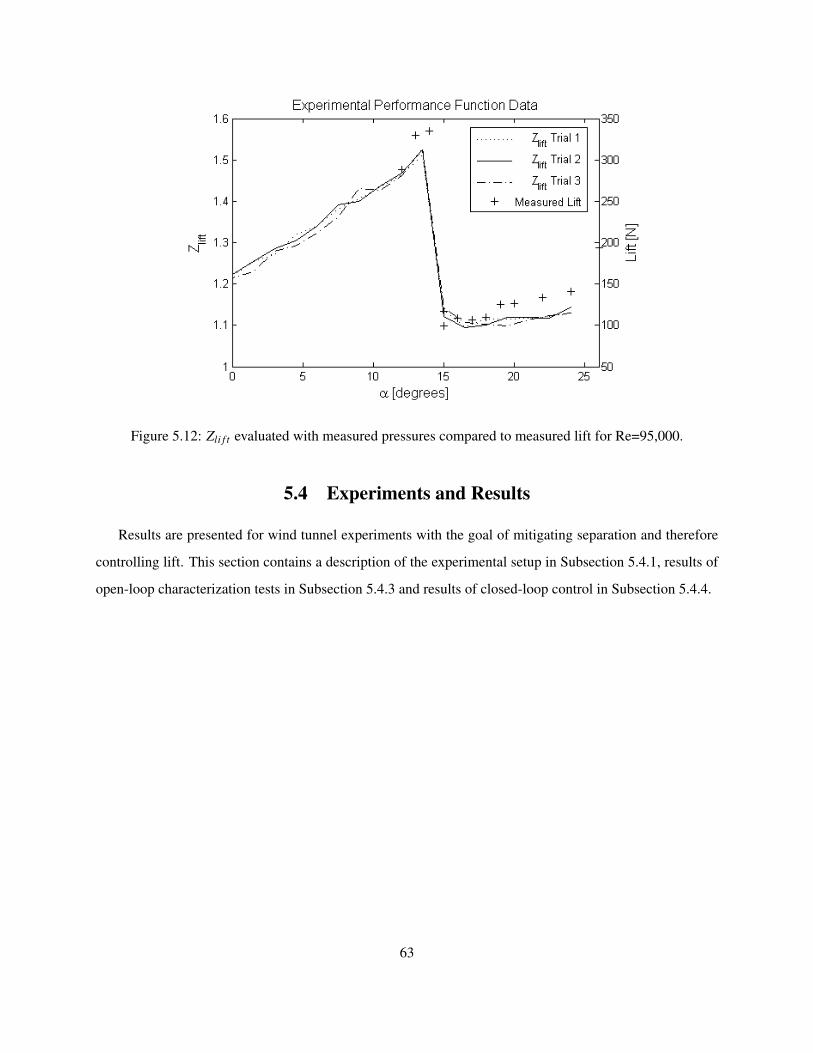
Figure 5.12: Zli f t evaluated with measured pressures compared to measured lift for Re=95,000.
5.4 Experiments and Results
Results are presented for wind tunnel experiments with the goal of mitigating separation and therefore
controlling lift. This section contains a description of the experimental setup in Subsection 5.4.1, results of
open-loop characterization tests in Subsection 5.4.3 and results of closed-loop control in Subsection 5.4.4.
63
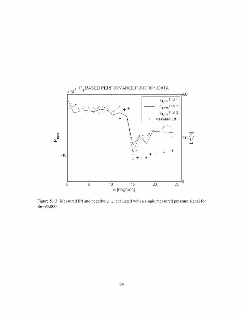
Figure 5.13: Measured lift and negative prms evaluated with a single measured pressure signal forRe=95,000.
64
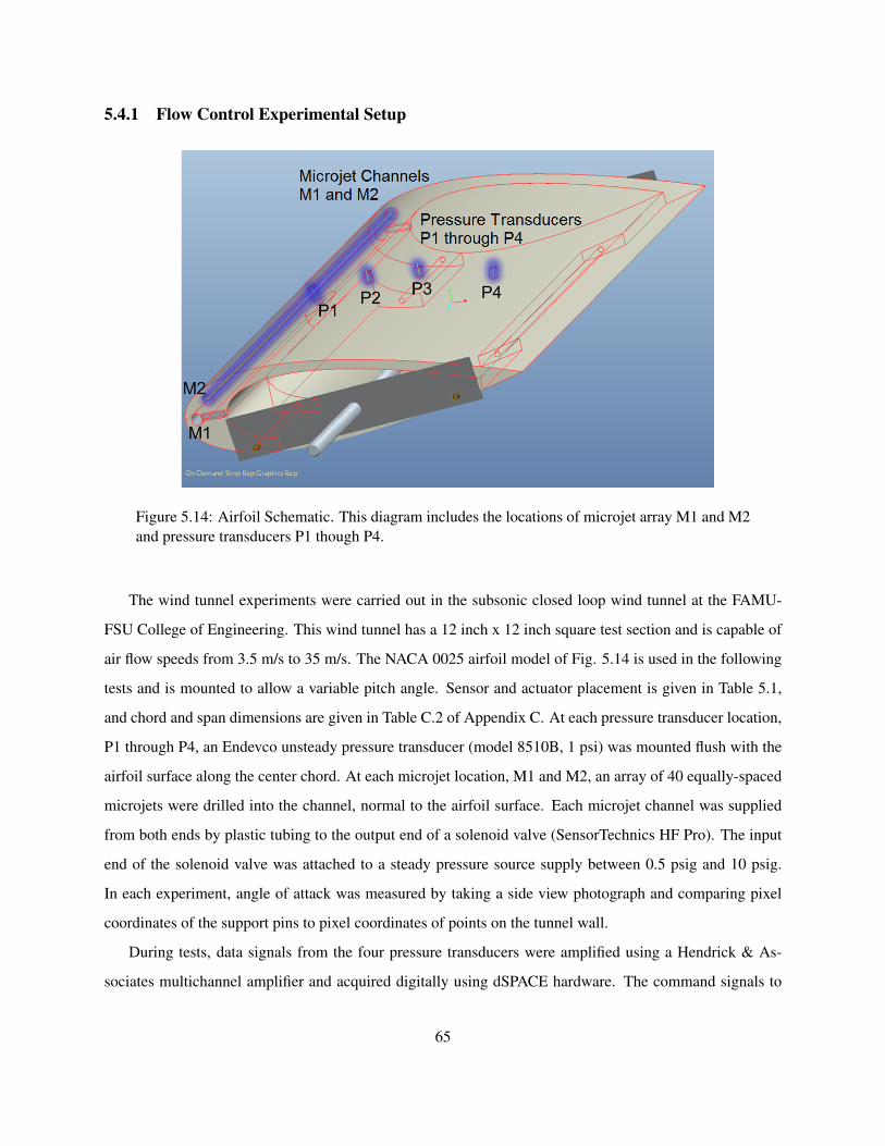
5.4.1 Flow Control Experimental Setup
Figure 5.14: Airfoil Schematic. This diagram includes the locations of microjet array M1 and M2and pressure transducers P1 though P4.
The wind tunnel experiments were carried out in the subsonic closed loop wind tunnel at the FAMU-
FSU College of Engineering. This wind tunnel has a 12 inch x 12 inch square test section and is capable of
air flow speeds from 3.5 m/s to 35 m/s. The NACA 0025 airfoil model of Fig. 5.14 is used in the following
tests and is mounted to allow a variable pitch angle. Sensor and actuator placement is given in Table 5.1,
and chord and span dimensions are given in Table C.2 of Appendix C. At each pressure transducer location,
P1 through P4, an Endevco unsteady pressure transducer (model 8510B, 1 psi) was mounted flush with the
airfoil surface along the center chord. At each microjet location, M1 and M2, an array of 40 equally-spaced
microjets were drilled into the channel, normal to the airfoil surface. Each microjet channel was supplied
from both ends by plastic tubing to the output end of a solenoid valve (SensorTechnics HF Pro). The input
end of the solenoid valve was attached to a steady pressure source supply between 0.5 psig and 10 psig.
In each experiment, angle of attack was measured by taking a side view photograph and comparing pixel
coordinates of the support pins to pixel coordinates of points on the tunnel wall.
During tests, data signals from the four pressure transducers were amplified using a Hendrick & As-
sociates multichannel amplifier and acquired digitally using dSPACE hardware. The command signals to
65

Table 5.1: Chord Locations of Microjet exits and Transducers.
Component M1 M2 P1 P2 P3 P4x/c 0.0 0.063 0.127 0.300 0.452 0.667
Figure 5.15: Buffer Circuit Diagram . The buffer circuit amplifies an input voltage signal so thatthe output voltage has sufficient current to drive the solenoid valves.
pressure transducers were sent from dSPACE and amplified using the op-amp buffer circuit of Fig. 5.4.1. In
open and closed loop testing, the single-input cases used only microjet array M2, and the two-input cases
used both arrays M1 and M2, supplied independently by two solenoid valves.
5.4.2 Particle Image Velocimetry
Two-Component Particle Image Velocimetry (PIV) was used in order to quantitatively examine the
flow field and provide evidence of reattachment of the separated flow. Because surface mounted unsteady
pressure sensors were in operation during PIV acquisition, a seeding fluid which left little to no residue on
the sensors was needed. For this application, Di-Ethyl-Hexyl-Sebacat (DEHS) was used with a Laskin type
seeder; nominal particle diameter was ∼1 µm. A 200 mJ, pulsed, Quantel R© Nd:YAG laser illumined the
seeded flow field of interest on the suction side of the airfoil. The laser sheet was formed by passing the
beam through LaVision sheet forming optics and expanded by a cylindrical lens; the optics were adjusted to
achieve a laser sheet thickness of ∼1 mm throughout the measurement domain. The spanwise location of
the laser sheet was approximately at the airfoil centerline. Due to the unsteady pressure sensors installed at
66
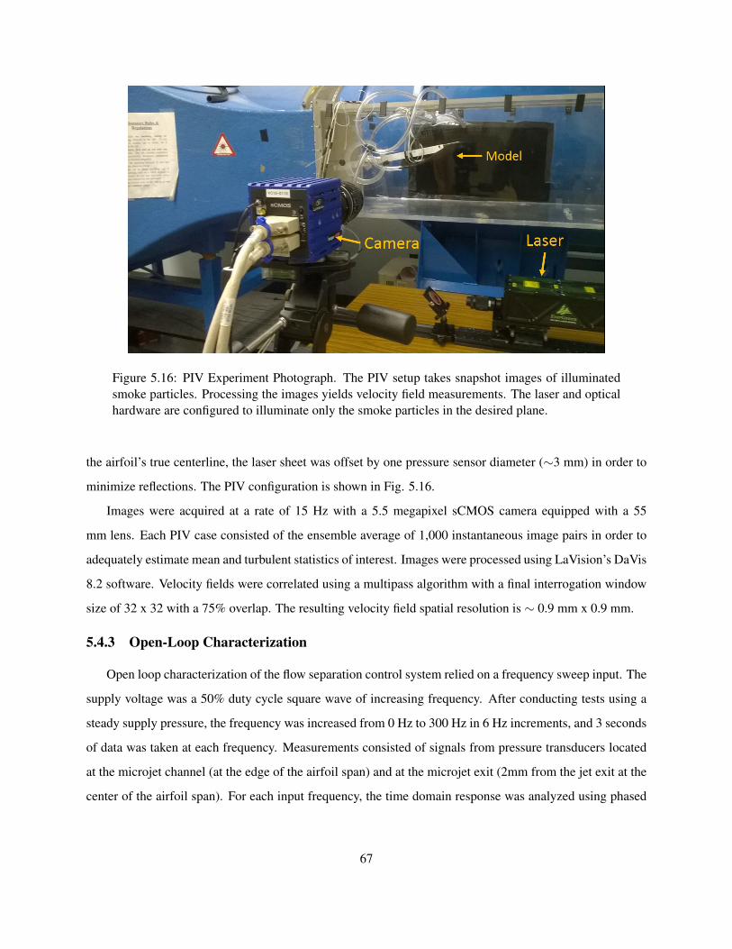
Figure 5.16: PIV Experiment Photograph. The PIV setup takes snapshot images of illuminatedsmoke particles. Processing the images yields velocity field measurements. The laser and opticalhardware are configured to illuminate only the smoke particles in the desired plane.
the airfoil’s true centerline, the laser sheet was offset by one pressure sensor diameter (∼3 mm) in order to
minimize reflections. The PIV configuration is shown in Fig. 5.16.
Images were acquired at a rate of 15 Hz with a 5.5 megapixel sCMOS camera equipped with a 55
mm lens. Each PIV case consisted of the ensemble average of 1,000 instantaneous image pairs in order to
adequately estimate mean and turbulent statistics of interest. Images were processed using LaVision’s DaVis
8.2 software. Velocity fields were correlated using a multipass algorithm with a final interrogation window
size of 32 x 32 with a 75% overlap. The resulting velocity field spatial resolution is ∼ 0.9 mm x 0.9 mm.
5.4.3 Open-Loop Characterization
Open loop characterization of the flow separation control system relied on a frequency sweep input. The
supply voltage was a 50% duty cycle square wave of increasing frequency. After conducting tests using a
steady supply pressure, the frequency was increased from 0 Hz to 300 Hz in 6 Hz increments, and 3 seconds
of data was taken at each frequency. Measurements consisted of signals from pressure transducers located
at the microjet channel (at the edge of the airfoil span) and at the microjet exit (2mm from the jet exit at the
center of the airfoil span). For each input frequency, the time domain response was analyzed using phased
67
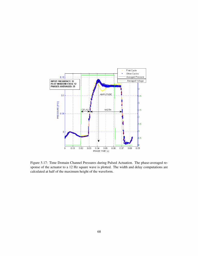
Figure 5.17: Time Domain Channel Pressures during Pulsed Actuation. The phase-averaged re-sponse of the actuator to a 12 Hz square wave is plotted. The width and delay computations arecalculated at half of the maximum height of the waveform.
68

0 50 100 150 200 250 30010−3
10−2
10−1
100
PRMS
: MICROJET CHANNEL PRESSURE
INPUT FREQUENCY [Hz]
OU
TP
UT
RO
OT
ME
AN
SQ
UA
RE
PR
ES
SU
RE
[PS
I]
Source P0 = 0.65
Source P0 = 0.8
Source P0 = 1
Source P0 = 1.2
Source P0 = 1.35
Source P0 = 1.5
Source P0 = 1.65
Source P0 = 1.8
Source P0 = 2
INCREASING P0
NOISE FLOOR
Figure 5.18: Frequency Domain Channel Pressures during Pulsed Actuation. The response of theactuator to frequency inputs is plotted.This plot displays the response measured at the microjetchannel for several different source pressures P0.
69
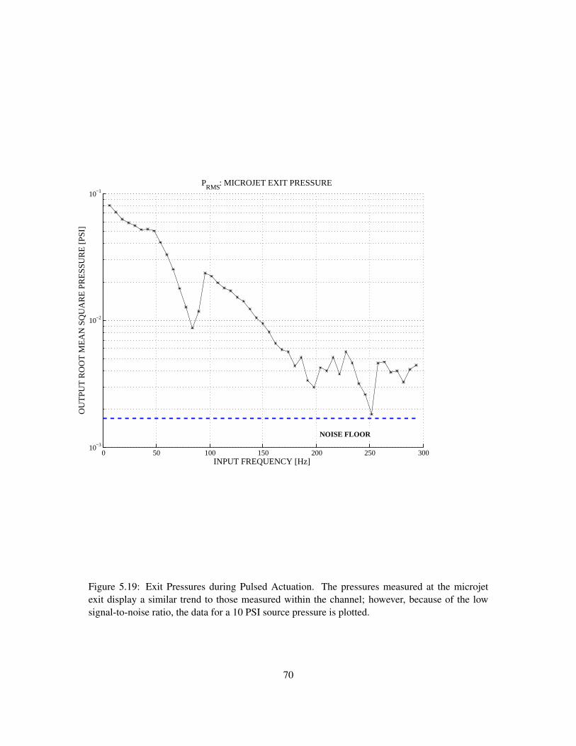
0 50 100 150 200 250 30010−3
10−2
10−1
PRMS
: MICROJET EXIT PRESSURE
INPUT FREQUENCY [Hz]
OU
TP
UT
RO
OT
ME
AN
SQ
UA
RE
PR
ES
SU
RE
[PS
I]
NOISE FLOOR
Figure 5.19: Exit Pressures during Pulsed Actuation. The pressures measured at the microjetexit display a similar trend to those measured within the channel; however, because of the lowsignal-to-noise ratio, the data for a 10 PSI source pressure is plotted.
70
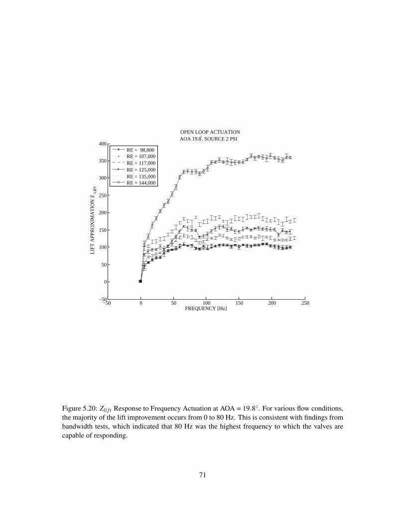
−50 0 50 100 150 200 250−50
0
50
100
150
200
250
300
350
400
OPEN LOOP ACTUATION AOA 19.8°, SOURCE 2 PSI
FREQUENCY [Hz]
LIF
T A
PP
RO
XIM
AT
ION
Z LI
FT
RE = 98,800RE = 107,000RE = 117,000RE = 125,000RE = 135,000RE = 144,000
Figure 5.20: Zli f t Response to Frequency Actuation at AOA = 19.8◦. For various flow conditions,the majority of the lift improvement occurs from 0 to 80 Hz. This is consistent with findings frombandwidth tests, which indicated that 80 Hz was the highest frequency to which the valves arecapable of responding.
71
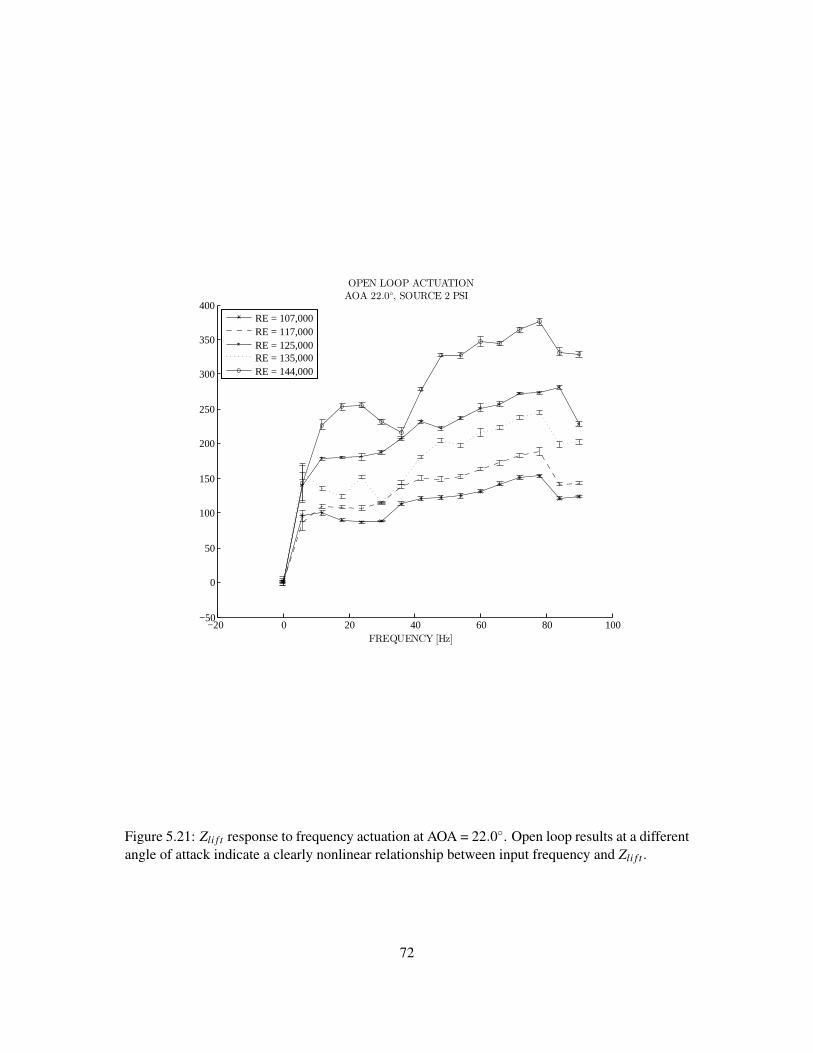
−20 0 20 40 60 80 100−50
0
50
100
150
200
250
300
350
400
OPEN LOOP ACTUATIONAOA 22.0◦, SOURCE 2 PSI
FREQUENCY [Hz]
RE = 107,000RE = 117,000RE = 125,000RE = 135,000RE = 144,000
Figure 5.21: Zli f t response to frequency actuation at AOA = 22.0◦. Open loop results at a differentangle of attack indicate a clearly nonlinear relationship between input frequency and Zli f t .
72
averaged data, such as the data plotted in Fig. 5.17 for the data collected during 12 Hz excitation. From
these phase averaged curves, the amplitude, width, and time delay between voltage excitation and pressure
response were calculated, as displayed in the figure. The delay and width of the waveform were computed
at 50
The data was sampled at 2 kHz, and time and frequency domain analysis was performed on these mea-
surements. From 0 to approximately 80 Hz, the pressure output frequency is identical to the voltage excita-
tion frequency. Above 80 Hz, mode switching occurs due to the dynamics of the solenoid valve. The valve,
which is designed for 30 Hz operation, switches primarily between the input frequency and 12 of the input
frequency.
Microjet exit pressure data is plotted in Fig. 5.19. In order to attain reasonable signal-to-noise ratio
(SNR) at the jet exit, the source pressure was increased to 10 psi. The pressure data collected at the microjet
exit (Fig. 5.19(b)) displayed similar trends to the data collected at the microjet channel (Fig. 5.19(a)).
In addition to bench top characterization, the open loop response of the overall system was measured in
the wind tunnel. The input for these tests was the solenoid valve voltage frequency, and the output was Zli f t ,
the lift based performance function computed from the transducer measurements at locations P1 through P4.
This performance function, derived in prior research [62], uses the four pressure signals to approximate lift
changes, weighting each sensor reading based on sensor spacing and airfoil geometry. For the NACA 0025
with sensors located as indicated in Table 5.1, Zli f t may be computed as
Zli f t =N
∑i=1
wi pi, (5.15)
with the weights wi given in Table C.2 of Appendix C. In the state vector of Eq. (5.6), each yk represents
a Zli f t measurement, and each uk represents a voltage frequency supplied to the solenoid valve for microjet
channel M2. Changes in the command voltage frequency were observed to cause changes in the steady state
value of Zli f t . After each 6 Hz frequency increment, data was collected after the system reached a steady
state. The data is presented in Figs. 5.20 and 5.21. Evidence of an actual change in lift as Zli f t changes
is given in the cp plots of Fig. 5.22. These discrete cp measurements suggest that the magnitude of the
area under the curve increases when going from 0 Hz to 72 Hz, which corresponds to greater suction on the
upper surface and higher lift. Further evidence includes observations of separation reduction indicated by
alignment of tufts on the airfoil surface as well as the generation of significant moments that were able to
rotate the airfoil setup when the microjets were actuated without the shaft clamped in place. Additionally, the
73
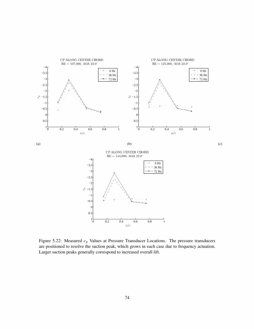
(a)
0 0.2 0.4 0.6 0.8 1
−4
−3.5
−3
−2.5
−2
−1.5
−1
−0.5
0
0.5
1
c p
x/c
CPALONG CENTER CHORD
RE = 107,000, AOA 22.0◦
0 Hz36 Hz72 Hz
(b)
0 0.2 0.4 0.6 0.8 1
−4
−3.5
−3
−2.5
−2
−1.5
−1
−0.5
0
0.5
1c p
x/c
CPALONG CENTER CHORD
RE = 125,000, AOA 22.0◦
0 Hz36 Hz72 Hz
(c)
0 0.2 0.4 0.6 0.8 1
−4
−3.5
−3
−2.5
−2
−1.5
−1
−0.5
0
0.5
1
c p
x/c
CPALONG CENTER CHORD
RE = 144,000, AOA 22.0◦
0 Hz36 Hz72 Hz
Figure 5.22: Measured cp Values at Pressure Transducer Locations. The pressure transducersare positioned to resolve the suction peak, which grows in each case due to frequency actuation.Larger suction peaks generally correspond to increased overall lift.
74

PIV measurements that are included in the following section provide definitive evidence of the effectiveness
of the microjet actuators to mitigate separation. Momentum coefficients cµ in these experiments ranged
from 0.33 (higher Reynolds number tests) to 0.5 (lower Reynolds number tests), since the typical microjet
velocity was approximately 5 m/s.
5.4.4 Closed-Loop Control
Frequency sweeps as mentioned above were used to train the neural network and represent the input-
output behavior of the system with a nonlinear model. Using a model initialized with sweep data, Adaptive
SBMPC was applied to perform closed loop control. During the 30-second learning phase (not plotted),
the identification algorithm was enabled, but the control algorithm was disabled. During the control phase,
both the controller and identification were enabled and produced successful tracking of the desired reference
value of Zli f t . In each experiment, the reference value was commanded manually, and the control system
automatically made the input adjustements necessary to drive the measured Zli f t signal to match the de-
sired reference signal. The tuning parameters selected for the identification and control algorithms are given
respectively in Figures D.1 and D.3 of Appendix D. In the plots of Figs. 5.23 through 5.26, the Zli f t was
normalized (divided by 100) to match the order of magnitude of the input space. This type of scaling is com-
monly applied [33] when using neural networks so that inverted matrices are numerically well-conditioned.
Reference tracking capability is demonstrated for a variety of reference trajectories. Figs. 5.23 and 5.24
indicate with an arrow the time at which control was activated. In the subsequent figures, the controller is
already active at time zero.
These results demonstrate the capability to not only maximize lift, but also control lift by commanding
intermediate values. In Fig. 5.23, the commanded reference signal (dashed line) is constant, which means
the control system was configured to increase and hold Zli f t constant. For this case, the momentum ratio cµ
of microjet momentum to free stream momentum is 0.4 and the Reynolds number is 125,000. The actual
ouput signal (solid line) achieves the commanded increase-and-hold behavior. In Fig. 5.24, the commanded
reference was manually stepped downwards, in order to demonstrate the ability of the control system to
decrease Zli f t when desired. This test was also configured with AOA= 20◦, RE= 125,000, and cµ=0.4. Fig
5.25 displays similar results and includes both upward and downward stepwise motion, again with AOA=
20◦, RE= 125,000, and cµ=0.4. For the case shown in Fig 5.26, the neural network was trained at a Reynolds
number of 125,000, but control is demonstrated for a Reynolds number of 150,000. In this test case, the
momentum coefficient cµ is 0.33. Some prediction error, indicated by the departure of the dotted line from
75
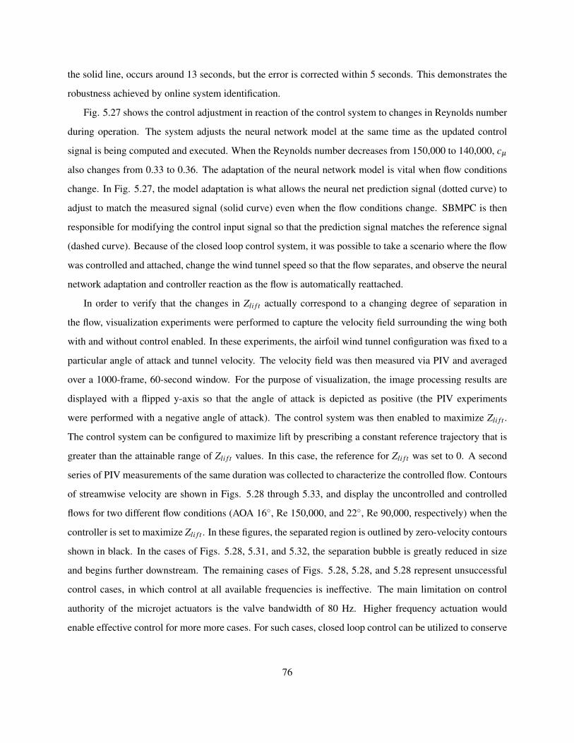
the solid line, occurs around 13 seconds, but the error is corrected within 5 seconds. This demonstrates the
robustness achieved by online system identification.
Fig. 5.27 shows the control adjustment in reaction of the control system to changes in Reynolds number
during operation. The system adjusts the neural network model at the same time as the updated control
signal is being computed and executed. When the Reynolds number decreases from 150,000 to 140,000, cµ
also changes from 0.33 to 0.36. The adaptation of the neural network model is vital when flow conditions
change. In Fig. 5.27, the model adaptation is what allows the neural net prediction signal (dotted curve) to
adjust to match the measured signal (solid curve) even when the flow conditions change. SBMPC is then
responsible for modifying the control input signal so that the prediction signal matches the reference signal
(dashed curve). Because of the closed loop control system, it was possible to take a scenario where the flow
was controlled and attached, change the wind tunnel speed so that the flow separates, and observe the neural
network adaptation and controller reaction as the flow is automatically reattached.
In order to verify that the changes in Zli f t actually correspond to a changing degree of separation in
the flow, visualization experiments were performed to capture the velocity field surrounding the wing both
with and without control enabled. In these experiments, the airfoil wind tunnel configuration was fixed to a
particular angle of attack and tunnel velocity. The velocity field was then measured via PIV and averaged
over a 1000-frame, 60-second window. For the purpose of visualization, the image processing results are
displayed with a flipped y-axis so that the angle of attack is depicted as positive (the PIV experiments
were performed with a negative angle of attack). The control system was then enabled to maximize Zli f t .
The control system can be configured to maximize lift by prescribing a constant reference trajectory that is
greater than the attainable range of Zli f t values. In this case, the reference for Zli f t was set to 0. A second
series of PIV measurements of the same duration was collected to characterize the controlled flow. Contours
of streamwise velocity are shown in Figs. 5.28 through 5.33, and display the uncontrolled and controlled
flows for two different flow conditions (AOA 16◦, Re 150,000, and 22◦, Re 90,000, respectively) when the
controller is set to maximize Zli f t . In these figures, the separated region is outlined by zero-velocity contours
shown in black. In the cases of Figs. 5.28, 5.31, and 5.32, the separation bubble is greatly reduced in size
and begins further downstream. The remaining cases of Figs. 5.28, 5.28, and 5.28 represent unsuccessful
control cases, in which control at all available frequencies is ineffective. The main limitation on control
authority of the microjet actuators is the valve bandwidth of 80 Hz. Higher frequency actuation would
enable effective control for more more cases. For such cases, closed loop control can be utilized to conserve
76
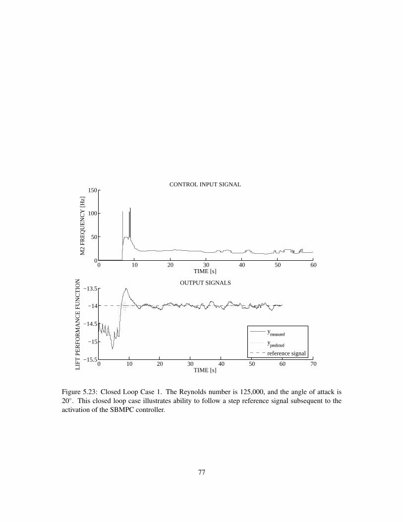
0 10 20 30 40 50 600
50
100
150CONTROL INPUT SIGNAL
TIME [s]
M2
FR
EQ
UE
NC
Y [H
z]
0 10 20 30 40 50 60 70−15.5
−15
−14.5
−14
−13.5OUTPUT SIGNALS
TIME [s]LIF
T P
ER
FO
RM
AN
CE
FU
NC
TIO
N
ymeasured
ypredicted
reference signal
Figure 5.23: Closed Loop Case 1. The Reynolds number is 125,000, and the angle of attack is20◦. This closed loop case illustrates ability to follow a step reference signal subsequent to theactivation of the SBMPC controller.
77
0 10 20 30 40 50 600
50
100
150
200
250CONTROL INPUT SIGNAL
TIME [s]
M2
FR
EQ
UE
NC
Y [H
z]
0 10 20 30 40 50 60−15
−14.5
−14
−13.5
−13OUTPUT SIGNALS
TIME [s]LIF
T P
ER
FO
RM
AN
CE
FU
NC
TIO
N
ymeasured
ypredicted
reference signal
Figure 5.24: Closed Loop Case 2. The Reynolds number is 125,000, and the angle of attack is20◦. This closed loop case illustrates the ability to command intermediate vales of Zli f t .
78
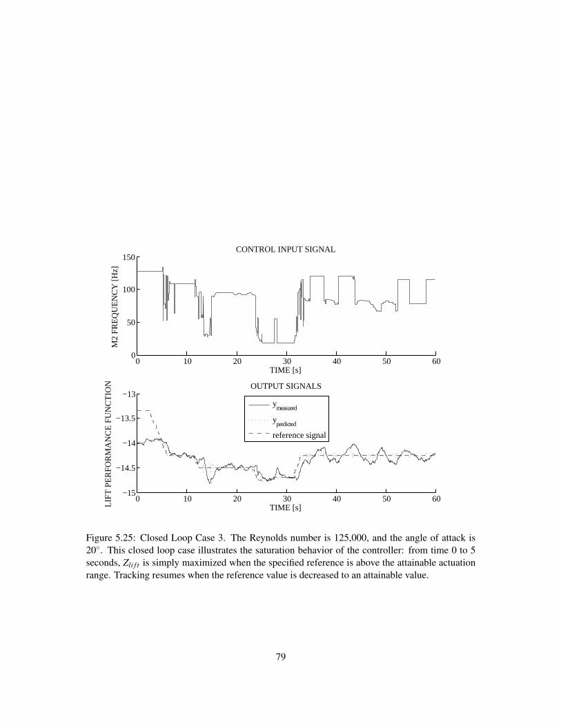
0 10 20 30 40 50 600
50
100
150CONTROL INPUT SIGNAL
TIME [s]
M2
FR
EQ
UE
NC
Y [H
z]
0 10 20 30 40 50 60−15
−14.5
−14
−13.5
−13OUTPUT SIGNALS
TIME [s]LIF
T P
ER
FO
RM
AN
CE
FU
NC
TIO
N
y
measured
ypredicted
reference signal
Figure 5.25: Closed Loop Case 3. The Reynolds number is 125,000, and the angle of attack is20◦. This closed loop case illustrates the saturation behavior of the controller: from time 0 to 5seconds, Zli f t is simply maximized when the specified reference is above the attainable actuationrange. Tracking resumes when the reference value is decreased to an attainable value.
79
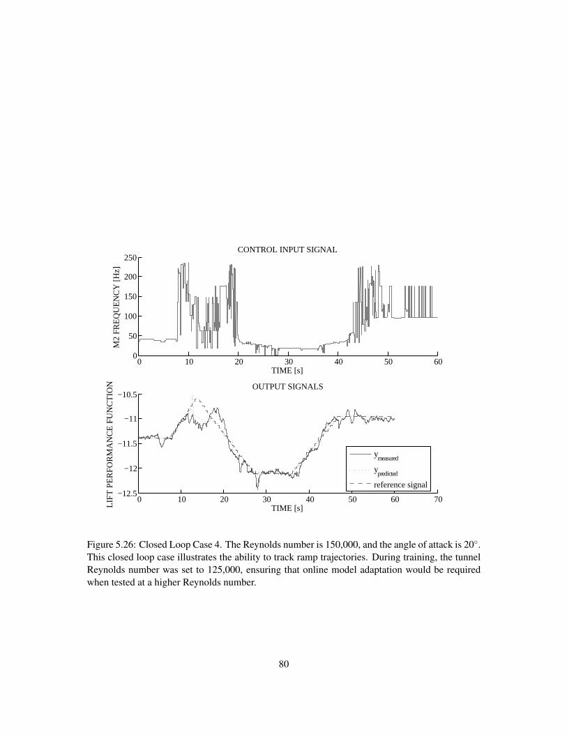
0 10 20 30 40 50 600
50
100
150
200
250CONTROL INPUT SIGNAL
TIME [s]
M2
FR
EQ
UE
NC
Y [H
z]
0 10 20 30 40 50 60 70−12.5
−12
−11.5
−11
−10.5OUTPUT SIGNALS
TIME [s]LIF
T P
ER
FO
RM
AN
CE
FU
NC
TIO
N
ymeasured
ypredicted
reference signal
Figure 5.26: Closed Loop Case 4. The Reynolds number is 150,000, and the angle of attack is 20◦.This closed loop case illustrates the ability to track ramp trajectories. During training, the tunnelReynolds number was set to 125,000, ensuring that online model adaptation would be requiredwhen tested at a higher Reynolds number.
80
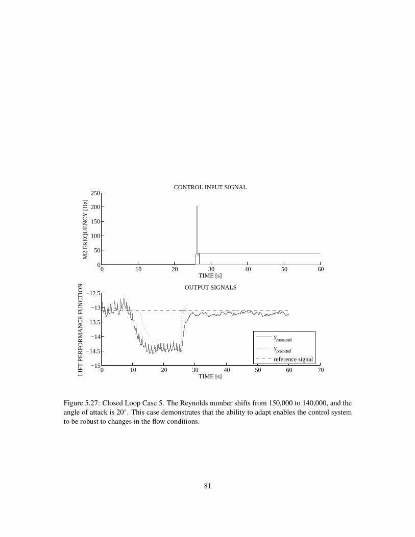
0 10 20 30 40 50 600
50
100
150
200
250CONTROL INPUT SIGNAL
TIME [s]
M2
FR
EQ
UE
NC
Y [H
z]
0 10 20 30 40 50 60 70−15
−14.5
−14
−13.5
−13
−12.5OUTPUT SIGNALS
TIME [s]LIF
T P
ER
FO
RM
AN
CE
FU
NC
TIO
N
ymeasured
ypredicted
reference signal
Figure 5.27: Closed Loop Case 5. The Reynolds number shifts from 150,000 to 140,000, and theangle of attack is 20◦. This case demonstrates that the ability to adapt enables the control systemto be robust to changes in the flow conditions.
81
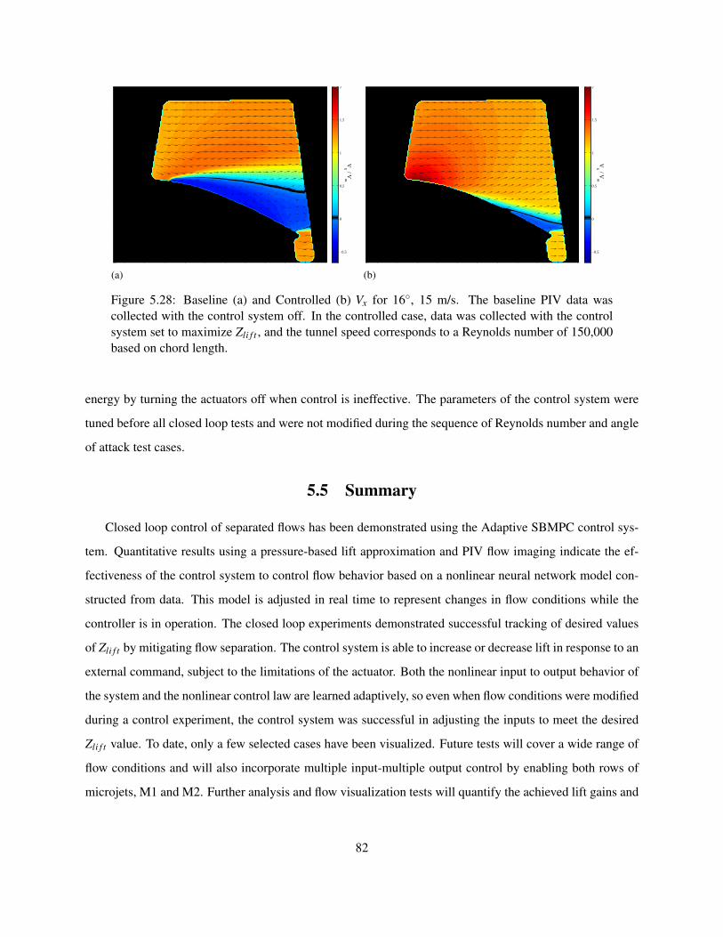
(a)
Vx / V
∞
0
20
40
60
80
100
120
140
160
−0.5
0
0.5
1
1.5
2
(b)
Vx / V
∞
0
20
40
60
80
100
120
140
160
−0.5
0
0.5
1
1.5
2
Figure 5.28: Baseline (a) and Controlled (b) Vx for 16◦, 15 m/s. The baseline PIV data wascollected with the control system off. In the controlled case, data was collected with the controlsystem set to maximize Zli f t , and the tunnel speed corresponds to a Reynolds number of 150,000based on chord length.
energy by turning the actuators off when control is ineffective. The parameters of the control system were
tuned before all closed loop tests and were not modified during the sequence of Reynolds number and angle
of attack test cases.
5.5 Summary
Closed loop control of separated flows has been demonstrated using the Adaptive SBMPC control sys-
tem. Quantitative results using a pressure-based lift approximation and PIV flow imaging indicate the ef-
fectiveness of the control system to control flow behavior based on a nonlinear neural network model con-
structed from data. This model is adjusted in real time to represent changes in flow conditions while the
controller is in operation. The closed loop experiments demonstrated successful tracking of desired values
of Zli f t by mitigating flow separation. The control system is able to increase or decrease lift in response to an
external command, subject to the limitations of the actuator. Both the nonlinear input to output behavior of
the system and the nonlinear control law are learned adaptively, so even when flow conditions were modified
during a control experiment, the control system was successful in adjusting the inputs to meet the desired
Zli f t value. To date, only a few selected cases have been visualized. Future tests will cover a wide range of
flow conditions and will also incorporate multiple input-multiple output control by enabling both rows of
microjets, M1 and M2. Further analysis and flow visualization tests will quantify the achieved lift gains and
82
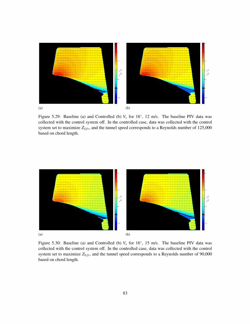
(a)
Vx / V
∞
0
20
40
60
80
100
120
140
160
−0.5
0
0.5
1
1.5
2
2.5
(b)
V
x / V∞
0
20
40
60
80
100
120
140
160
−0.5
0
0.5
1
1.5
2
2.5
Figure 5.29: Baseline (a) and Controlled (b) Vx for 16◦, 12 m/s. The baseline PIV data wascollected with the control system off. In the controlled case, data was collected with the controlsystem set to maximize Zli f t , and the tunnel speed corresponds to a Reynolds number of 125,000based on chord length.
(a)
Vx / V
∞
0
20
40
60
80
100
120
140
160
−0.5
0
0.5
1
1.5
2
2.5
(b)
Vx / V
∞
0
20
40
60
80
100
120
140
160
−0.5
0
0.5
1
1.5
2
2.5
Figure 5.30: Baseline (a) and Controlled (b) Vx for 16◦, 15 m/s. The baseline PIV data wascollected with the control system off. In the controlled case, data was collected with the controlsystem set to maximize Zli f t , and the tunnel speed corresponds to a Reynolds number of 90,000based on chord length.
83

(a)
Vx / V
∞
0
20
40
60
80
100
120
140
160
−0.5
0
0.5
1
1.5
2
2.5
(b)
V
x / V∞
0
20
40
60
80
100
120
140
160
−0.5
0
0.5
1
1.5
2
2.5
Figure 5.31: Baseline (a) and Controlled (b) Vx for 22◦, 11 m/s. The baseline PIV data wascollected with the control system off. In the controlled case, data was collected with the controlsystem set to maximize Zli f t , and the tunnel speed corresponds to a Reynolds number of 90,000based on chord length.
(a)
Vx / V
∞
0
20
40
60
80
100
120
140
160
−0.5
0
0.5
1
1.5
2
2.5
(b)
Vx / V
∞
0
20
40
60
80
100
120
140
160
−0.5
0
0.5
1
1.5
2
2.5
Figure 5.32: Baseline (a) and Controlled (b) Vx for 22◦, 12 m/s. The baseline PIV data wascollected with the control system off. In the controlled case, data was collected with the controlsystem set to maximize Zli f t , and the tunnel speed corresponds to a Reynolds number of 125,000based on chord length.
84
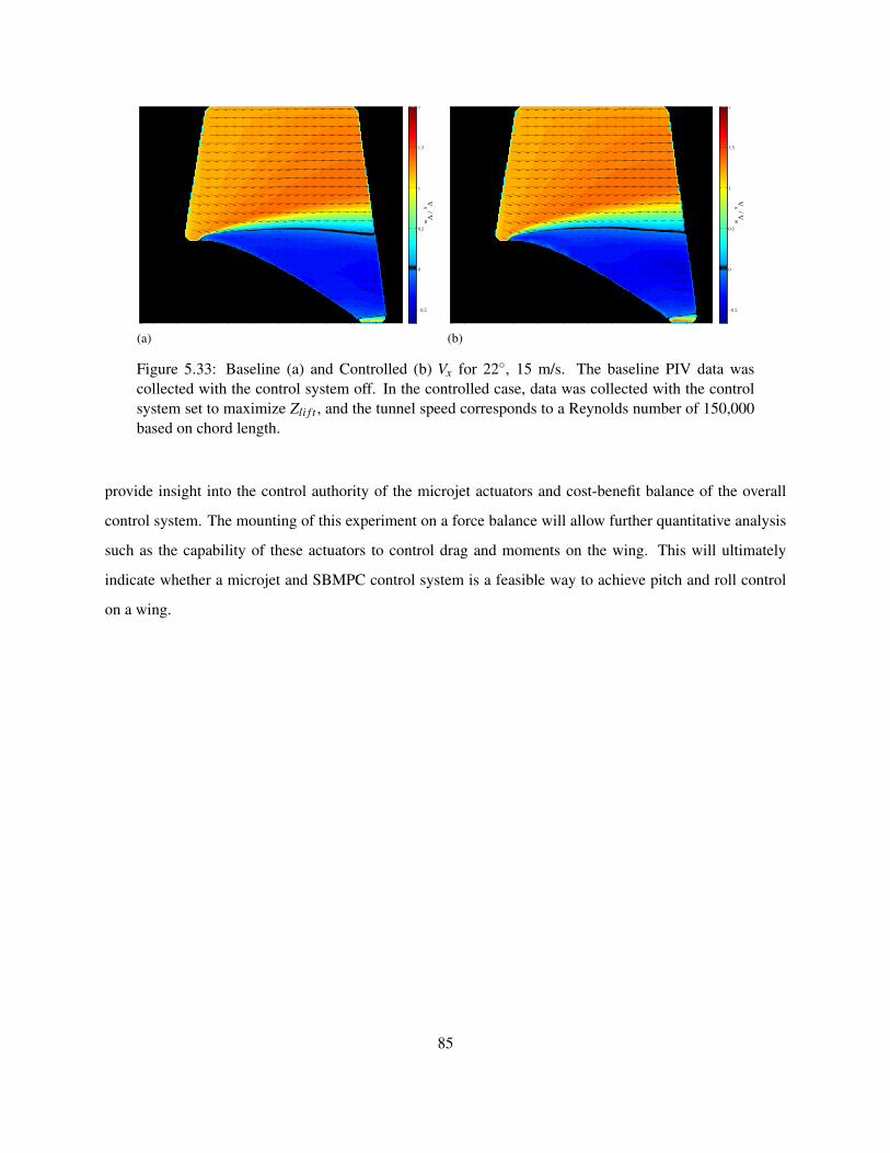
(a)
Vx / V
∞
0
20
40
60
80
100
120
140
160
−0.5
0
0.5
1
1.5
2
(b)
Vx / V
∞
0
20
40
60
80
100
120
140
160
−0.5
0
0.5
1
1.5
2
Figure 5.33: Baseline (a) and Controlled (b) Vx for 22◦, 15 m/s. The baseline PIV data wascollected with the control system off. In the controlled case, data was collected with the controlsystem set to maximize Zli f t , and the tunnel speed corresponds to a Reynolds number of 150,000based on chord length.
provide insight into the control authority of the microjet actuators and cost-benefit balance of the overall
control system. The mounting of this experiment on a force balance will allow further quantitative analysis
such as the capability of these actuators to control drag and moments on the wing. This will ultimately
indicate whether a microjet and SBMPC control system is a feasible way to achieve pitch and roll control
on a wing.
85
CHAPTER 6
CONCLUDING REMARKS
6.1 Summary of Completed Research
The completed dissertation research includes development of simulation and experimental software,
testing in simulation of model-based adaptive control algorithms for simulated nonlinear systems, imple-
mentation in simulation and experiments of neural network identification approaches, and implementation
in simulation and experiments of SBMPC. The simulated study of coal power plant combustion served as a
proof of concept for the control system and also demonstrated MIMO results. The flow separation control
application demonstrated the real time implementation of the algorthms. Intermediate work, including the
characterization of the relationship between sensor signals and aerodynamic performance from experimen-
tal data and the development and validation of a lift-based performance function, are the types of enginering
tasks that would need to be performed when applyiing the general Adaptive SBMPC algorithm to various
real world applications. The software modules for MRAN and SBMPC algorithms have been compiled
and executed on dSPACE hardware (Solaris operating system) for real time execution. SBMPC controller
code has been implemented in C and adapted to the real-time framework to compile on dSPACE. Neural
network identification code has been implemented in MATLAB, translated to C, and implemented for real
time execution in dSPACE.
A dynamic simulation with multiple inputs and outputs was implemented to demonstrate the adaptive,
nonlinear, and constraint-handling capabilities of the Adaptive SBMPC method. This work investigated
a problem from process control literature and extends the problem to address MIMO and time-varying
systems. A custom implementation of Neural GPC was prepared in order to compare the performance of
Adaptive SBMPC with an existing method. The performance exceeds that of Neural GPC and requires less
computation time for each simulated example.
For the application to flow control, hardware construction was completed for incremental designs of
the NACA 0025 airfoil fitted with pressure transducers and microjet channels as well as a motor-pulley
system for repeatable angle of attack actuation in 0.3◦ increments. Two iterations of a pressure regulation
system have been constructed and used for all open loop SISO and MIMO tests, and successful feedback
86
control has been demonstrated on the wind tunnel experimental model. Efficacy of the control system was
verified with PIV imaging for selected feedback control cases. The same control system has been applied to
multiple flow condition configurations without altering the tuning parameters and has performed effectively
across a range of angles of attack and Reynolds Numbers, which demonstrates the robustness of the method
achieved through adaptation. The diversity of studied applications, including both flow control and power
plant control, demonstrates that the Adaptive SBMPC technique is suitable for diverse applications.
6.2 Future Work
Several areas for continued research that would bring this technology closer to implementation on real
industrial systems. These areas include computational speedups and additional applications. For the flow
control application, future work includes exploration of other sensors and actuators, and further experimen-
tation to demonstrate robustness.
6.2.1 Learning of Heuristics
One potential improvement to Adaptive SBMPC, the learning of A∗ search heuristics for general non-
linear systems, which would enable further computational improvements, are planned as future work. This
improved implementation will make use of past optimization cost information to speed up subsequent opti-
mizations for the same plant.
6.2.2 Parallel Implementation
Further computational improvement is possible using parallel computation. During SBMPO execution,
the majority of the the computational effort is spent on expansion of nodes. These expansions may be
computed in parallel in order to leverage the capabilities of multi-core CPU or GPU hardware. These
computation improvements will allow the application of Adaptive SBMPC to larger systems as well as
systems with fast real-time computation requirements.
6.2.3 Additional Applications
The techniques developed in this dissertation are applicable across several industries, and commercial
partnership and licensing opportunities are being explored in the power plant control and automotive engine
tuning. Discussions with Siemens Energy, Inc., have indicated that there is interest in the Adaptive SBMPC
technology for emissions control. Preliminary research results for Adaptive SBMPC have demonstrated that
87

the technique is applicable to power generation and emissions regulations. The application is control of
combustion in a coal-fired or gas-fired boiler, which has been demonstrated in simulation. Although smaller
plants are more numerous, large plants (200 MW and above) produce the majority of the nation’s energy
demands, and these are the most heavily regulated by the EPA.
The automotive engine industry, another target market, is also changing dramatically due to environ-
mental concerns, yet the industry has sustained growth over the past decade. Efficiency has long been a
driver for this industry, and with the rising price of fuel, this will remain a priority. Adaptive SBMPC is
a fast method that can be applied to carry out optimization of engine parameters, which leads to increased
efficiency and longevity of engine operations. With numerous parameters and a large search space, time-
consuming manual tuning, the current approach, results in suboptimal solutions. As a result, existing engines
are not achieving the best possible efficiency. As in the electric power industry, EPA regulation is a major
factor in the US automotive engine market. Cummins, for example, was the only company in the market to
meet the 2010 EPA standards for NOx emissions with their release of a 6.7-liter turbo diesel for the Dodge
Ram Heavy Duty pickup. Better efficiency and control of emissions will continue to be in high demand, as
environmental legislation and rising fuel prices continue to make innovation a necessity.
6.2.4 Future Flow Control Research
Because of the variety of new experimental actuators as well as new sensor concepts, future flow control
applications for Adaptive SBMPC are numerous. Some directions for future flow control research using
Adaptive SBMPC are given below.
High Frequency Actuation. The flow control actuation using solenoid valves produced actuator sig-
nals up to approximately 80 Hz, which allows for actuation relevant to large vortex shedding in the wake of
the airfoil. The frequencies produced by these actuators are not high enough, however, to interact with the
smaller-scale Kelvin Helmholtz vortex structures that form along the boundary layer, which occur on the
order of kilohertz at low Reynolds Numbers [45].
Performance Function Testing for Alternate Geometries. Studies using the NACA 0025 airfoil
geometry have produced favorable results in both simulation and experiment. In order to produce evidence
of the performance function’s wide applicability to airborne systems and turbomachinery, tests should be
performed with flat plate, NACA 0012, and asymmetric airfoil geometries. It is also possible to mount
88

pressure sensors across the airfoil surface in a spanwise array and use a performance function to measure
rolling moments on the airfoil.
Performance Function Testing in Challenging Environments. It is critical to know the capabilities
and limitations of a control system, especially of technologies that may be deployed in the future. We pro-
pose a series of tests that will demonstrate performance function effectiveness over a series of emulated
environmental effects. One such effect is loud broadband noise from an external source. It is hypothe-
sized that the lift based performance function will handle this disturbance better than an RMS performance
function because the lift based performance function uses the mean pressure, not its fluctuations, to de-
tect separation. Other environmental factors would include decreased microjet supply pressures or variable
humidity and fog.
89

APPENDIX A
SBMPO ALGORITHM PSEUDOCODE
The SBMPO Algorithm is listed here. Beginning with the root node that represents the system’s current
state, a graph is built by iteratively expanding the most promising node to generate B child nodes. Each
child node is assigned an input sample, which is propagated forward through the model to predict a state
for that node. The potential cost of reaching that state is used to prioritize the nodes and select the most
promising candidate for the next iteration of expansion.
90

Algorithm 1 Calculate input sequence U via SBMPO graph searchInsert root node into the queue withi← 0CE,i← 0ND,i← 0parenti← NULLxi← x0
Evaluate heuristic costCH,i← HEUR COST EVALPop the top node from the queuewhile (ND,top < N)∧ (i < MAX NODES) do
while CE,top = NULL doEvaluate edge costCE,top←CE,parent+EDGE COST EVALRe-insert node into queue, sorted by CE +CH
Pop the top node from the queueend whileExpand by Generating B child nodesfor j ∈ [i+1, i+B) do
Generate input space sampleu j←HALTON SEQUENCE LOOKUPIntegrate the modelx j←MODEL EVAL(u j,xtop)Evaluate heuristic costCH, j← HEUR COST EVALCE, j← NULLND, j← ND,top +1parent j← iInsert node j into queue, sorted by CH
end fori← i+BPop the top node from the queue
end whileConstruct the optimal input trajectoryj← topwhile ND, j > 0 do
U(ND, j−1) = u j
j← parent j
end while
91

APPENDIX B
SBMPO SOUNDNESS AND COMPLETENESS PROOF
This proof of soundness and completeness for the algorithm listed in Appendix A is loosely based on the
procedure in [35], in which soundness and completeness is derived for a different graph search algorithm. Its
culmination, Theorem B.0.6, guarantees that, subject to sufficient depth and breadth of sampling, SBMPO
will find a globally optimal solution.
Assumption B.0.1. The heuristic function is optimistic.
Assumption B.0.2. All reachable states have finite edge costs.
Assumption B.0.3. All edge costs are non-negative.
Lemma B.0.4. The Algorithm will terminate in a finite number of steps, returning a path of length N.
Proof.
The root node is inserted only once before the main algorithm loop begins. Each node, once expanded,
is not re-inserted into the queue, and new nodes (other than the root node) are only inserted by expansion
of a parent node. Therefore, each node in the graph is introduced no more than once. In the case in which
every parent node of depth ND is expanded, there are at most BND nodes of depth ND+1 placed in the queue.
No node of greater depth than the prediction horizon N can be generated, since the algorithm termination
clause would have been reached first. Including node depths 0 through N, there are at most L =∑NND=0 BND =
1−BN+1
1−B nodes in the entire graph. Each time through the loop, either a node edge cost is computed, a node is
expanded, or the algorithm terminates.
If a node edge cost is computed, the queue size is unchanged after that loop iteration (i.e., the node is
re-inserted). The number of items in the queue without a computed edge cost, however, decreases by 1.
Since each node is introduced no more than once and each edge cost is computed no more than once, the
algorithm must terminate before exceeding 2L loop iterations. The returned path is of length N because the
algorithm can only terminate upon selecting a path of length N.
92

Lemma B.0.5. The returned path’s total cost is less than or equal to that of any path in the graph of length
N.
Proof. (By Contradiction.)
Assume that for the selected path, there exists a path P− of length N in the graph with a lower cost than
the path returned by the algorithm. Therefore P− must not be represented from the queue. Otherwise, it
would have been selected instead of the returned path. The node representing selected path N+ must have
been at the top of the sorted queue (having the lowest total cost in the queue). Because all edge costs are
positive, and a node’s heuristic value is optimistic, every partial path contained in a path of length N will
have a cost less than or equal to the length-N path that contains it.
Let node N− represent the terminal node of the longest partial path of P− that was added to the queue.
This node must exist because all paths in the graph begin with the same root node, which represents the
initial state. Then N− must have lower total cost than the node N+ that was selected by the algorithm.
Therefore, N− must have been placed higher in the sorted queue and would have been expanded prior to
the selection of N+, but this yields a contradiction, because the children of node N− would include a node
representing a partial path of P− that is one edge longer that the path represented by N−. This is not possible
because we chose N− to be the longest partial path of P− that was added to the queue.
Theorem B.0.6 (Soundness and Completeness). Upon termination, the SBMPO algorithm will produce a
path of nodes representing a minimal cost trajectory among those represented by the graph.
Proof. This theorem follows from Lemmas B.0.4 and B.0.5.
93

APPENDIX C
LISTS OF SIMULATION AND EXPERIMENTPARAMETERS
Table C.1 gives the baseline parameters used in the simulated steam boiler. Table C.2 gives the parameters
describing the wind tunnel experiment configuration.
Table C.1: Simulation Parameters: Combustion
Symbol Parameter Value(s)
Vd Gas Production Constant 2.399×10⁻³ m3/kg
VO O2 Consumption Constant 1.543×10⁻³ m3/kg
x fC Fuel Carbon Fraction 0.8087
V Volume of Chamber 0.01 m3
Φmax Max Air Flow 1.833e-2 m3/s
T Control Period 10 s
τ Simulation Integration Step 1×10⁻⁴ s
94

Table C.2: Experiment Parameters: Flow Control
Symbol Parameter Value(s)
w1 p1 Weight -1.000
w2 p2 Weight -0.9781
w3 p3 Weight -0.9348
w4 p4 Weight -0.9126
c Chord Length 6 inches
b Span Length 11.5 inches
T Control Period 100 ms
P0 Microjet Source Pressure 0.5 to 10PSI,
Vjet Microjet Velocity (P0 = 2PSI)
5 m/s
95

APPENDIX D
LIST OF TUNING PARAMETER CHOICES
Tables D.1, D.2, D.3, and D.4 give the tuning parameters used in the simulation for each identification and
control method. Unless otherwise noted the same tuning parameters were used for all three cases. Tables
D.5 and D.6 give the tuning parameters used in the flow control experiment for the identification and control
methods.
Table D.1: MRAN Parameter Choices: Combustion Control
Symbol Parameter Value(s)
E1 Instantaneous Error Threshold 0.00209
E2 RMS Error Threshold 0.005
E3 Basis Vector Spacing Threshold 0.16
E3DEC E3 Geometric Decay Rate 0.9985
E3MIN E3 Decay Floor 0.03
M RMS Averaging Window 48
N∗ Max Hidden Units 480
κ Overlap Factor 10.0
q Kalman Step Parameter 0.5
p0 New Parameter Variance 5.0
R Assumed Sensor Noise Variance 0.0
Mp,1 Pruning Window 1 800
Mp,2 Pruning Window 2 2000
δp,1 Pruning Threshold 1 2×10⁻⁸
δp,2 Pruning Threshold 2 1×10⁻⁴
96

Table D.2: BPN Parameter Choices
Symbol Parameter Value(s)
NH Hidden Units 19, 39, 39∗
α Learning Rate 5.7
η Momentum Coefficient 5000,2778.7,2778.7∗
L Network Gain 0.007
M1 y1 Scaling Multiplier 6.0
B1 y1 Scaling Bias 0.0
M2 y2 Scaling Multiplier 105†
B2 y2 Scaling Bias 0.5†
M3 y3 Scaling Multiplier 2.0†
B3 y3 Scaling Bias 0.0†
∗ Case 1, Case 2, and Case 3, respectively.
† Only applicable to Cases 2 and 3.
Table D.3: SBMPC Parameter Choices: Combustion Control
Symbol Parameter Value(s)
B Branchout Factor 60
N Prediction Horizon 4
Nc Control Horizon 2
97

Table D.4: GPC Parameter Choices: Combustion Control
Symbol Parameter Value(s)
N Prediction Horizon 4
Nc Control Horizon 2
ε Solver Tolerance 10−6
Imax Max Newton Iterations 1500
s Constraint Sharpness 10−15
λ Damping Factor 4×10−3,9×109,9×109*
*Case 1, Case 2, and Case 3, respectively.
Table D.5: MRAN Parameter Choices: Flow Control
Symbol Parameter Value(s)
E1 Instantaneous Error Threshold 0.5
E2 RMS Error Threshold 2.0
E3 Basis Vector Spacing Threshold 2.0
E3DEC E3 Geometric Decay Rate 1.0
E3MIN E3 Decay Floor 2.0
M RMS Averaging Window 48
N∗ Max Hidden Units 120
κ Overlap Factor 1.0
q Kalman Step Parameter 0.5
p0 New Parameter Variance 5.0
R Assumed Sensor Noise Variance 0.0
Mp,1 Pruning Window 1 800
Mp,2 Pruning Window 2 2000
δp,1 Pruning Threshold 1 2×10⁻⁸
δp,2 Pruning Threshold 2 1×10⁻⁴
98

Table D.6: SBMPC Parameter Choices: Flow Control
Symbol Parameter Value(s)
B Branchout Factor 60
N Prediction Horizon 2
Nc Control Horizon 2
T Control Sample Period 100 ms
99
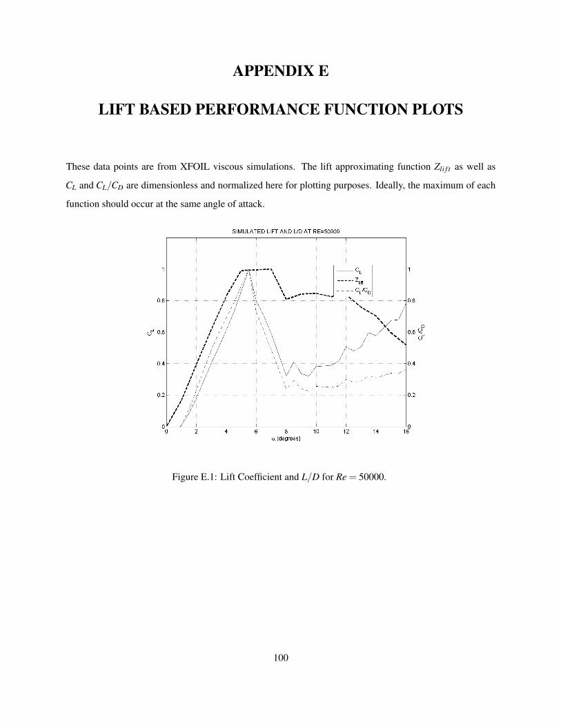
APPENDIX E
LIFT BASED PERFORMANCE FUNCTION PLOTS
These data points are from XFOIL viscous simulations. The lift approximating function Zli f t as well as
CL and CL/CD are dimensionless and normalized here for plotting purposes. Ideally, the maximum of each
function should occur at the same angle of attack.
Figure E.1: Lift Coefficient and L/D for Re = 50000.
100
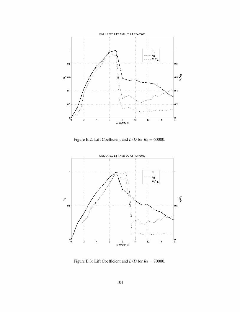
Figure E.2: Lift Coefficient and L/D for Re = 60000.
Figure E.3: Lift Coefficient and L/D for Re = 70000.
101

Figure E.4: Lift Coefficient and L/D for Re = 80000.
Figure E.5: Lift Coefficient and L/D for Re = 90000.
102
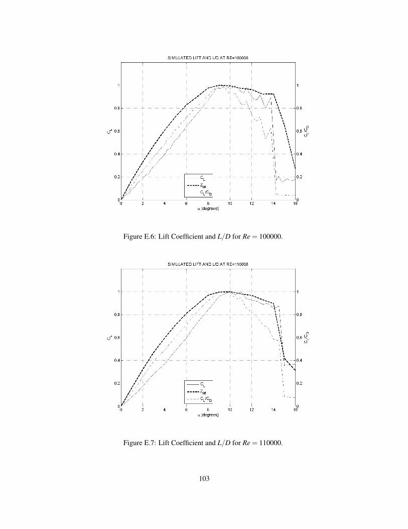
Figure E.6: Lift Coefficient and L/D for Re = 100000.
Figure E.7: Lift Coefficient and L/D for Re = 110000.
103
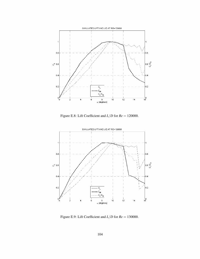
Figure E.8: Lift Coefficient and L/D for Re = 120000.
Figure E.9: Lift Coefficient and L/D for Re = 130000.
104
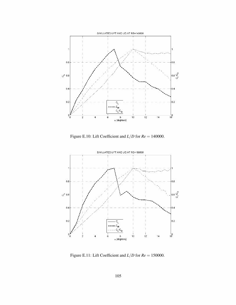
Figure E.10: Lift Coefficient and L/D for Re = 140000.
Figure E.11: Lift Coefficient and L/D for Re = 150000.
105
BIBLIOGRAPHY
[1] Motion planning for mobile robots via sampling-based model predictive optimization.
[2] A sequential learning scheme for function approximation using minimal radial basis function neuralnetworks. Neural computation, 9(2):461–478, 1997.
[3] Q&a: Epa regulation of greenhouse gas emissions from existing power plants. Center for Climate andEnergy Solutions, June 2014.
[4] Farrukh S. Alvi. Adaptive control of inlet separation using supersonic microjets. Technical report,NASA Langley Research Center, Hampton, VA.
[5] Alberto Bemporad and Manfred Morari. Robust model predictive control: A survey. In Robustness inidentification and control, pages 207–226. Springer, 1999.
[6] Rıdvan Berber and Costas Kravaris. Nonlinear model based process control, volume 353. Springer,1998.
[7] Lorenz T Biegler. A survey on sensitivity-based nonlinear model predictive control. In 10th IFACInternational Symposium on Dynamics and Control of Process Systems, pages 499–510, 2013.
[8] A Bitenc, J Cretnik, J Petrovcic, and S Strmcnik. Design and application of an industrial controller.Computing Control Engineering Journal, 3(1):29–34, 1992.
[9] EF Camacho, M Berenguel, and FR Rubio. Application of a gain scheduling generalized predictivecontroller to a solar power plant. Control Engineering Practice, 2(2):227–238, 1994.
[10] Louis Cattafesta, Ye Tian, and R. Mittal. Adaptive control of post-stall separated flow application toheavy vehicles. Springer Berlin Heidelberg Lecture Notes in Applied and Computational Mechanics,41(5):151–160, 2009.
[11] H Chi, M Mascagni, and T T Warnock. On the optimal halton sequence. Mathematics and Computersin Simulation, 70(1):9–21, 2005.
[12] Oscar Y. Chuy, Vikas Kumar, Frederick V. Holt III, Emmanuel G. Collins Jr., and Farrukh S. Alvi.Microjet-based separation control using a virtual sensor for degree of separation. In Florida Centerfor Advanced Aero-Propulsion Annual Technical Symposium, Tallahassee, Fl, August 2009. FCAAP.
[13] D W Clarke. Generalized predictive control. Automatica, 23(2):149–160, 1987.
[14] J Cretnik. Modern Automatic Combustion Control. Phd dissertation, Ljubljana School of Electricaland Computer Engineering, 1992.
106
[15] Jurij Cretnik. Modern automatic combustion control. 1993.
[16] I Culjak, A Sikanic, and V Koroman. Renewable energy sources in compliance of kyoto protocoltargets: Case study of 42 mw wind field. Energy and the Environment 2008 Vol 2, pages 89–99 464,2008.
[17] Daniel Delling, Peter Sanders, Dominik Schultes, and Dorothea Wagner. Engineering route planningalgorithms. In Algorithmics of large and complex networks, pages 117–139. Springer, 2009.
[18] Damion Dunlap, Wei Yu, Emmanuel G Collins, and Charmane V Caldwell. Motion planning for steephill climbing. In 2011 IEEE International Conference on Robotics and Automation, pages 707–714.IEEE, 2011.
[19] Damion D Dunlap, Charmane V Caldwell, and Emmanuel G Collins Jr. Nonlinear model predictivecontrol using sampling and goal-directed optimization. Mechanical Engineering, 16:1349–1356, 2010.
[20] M. Debiasi M. Samimy E. Caraballo, J. Little. Development and implementation of an experimentalbased reduced-order model for feedback control of subsonic cavity flows. Journal of Fluids Engineer-ing, 129(7):813–824, 2007.
[21] Christer Ericson. Real-time collision detection, volume 14. Elsevier Amsterdam/Boston, 2005.
[22] Julien Favier, Azeddine Kourta, and Gillian Leplat. Control of flow separation of a wing profile usingpiv measurements and pod analysis. In IUTAM Symposium on Flow Control with MEMS. IMFT -French National Institute of Mechanics of Toulouse, IUTAM, September 2006.
[23] Eduardo Gallestey, Alec Stothert, Marc Antoine, and Steve Morton. Model predictive control andthe optimization of power plant load while considering lifetime consumption. Power Systems, IEEETransactions on, 17(1):186–191, 2002.
[24] Alexandra Grancharova and Tor Arne Johansen. Explicit nonlinear model predictive control: theoryand applications, volume 429. Springer, 2012.
[25] Alexandra Grancharova, Ju Kocijan, and Tor A Johansen. Explicit stochastic predictive control ofcombustion plants based on gaussian process models. Automatica, 44(6):1621–1631, 2008.
[26] Alexandra Grancharova, Ju Kocijan, and Tor A Johansen. Explicit output-feedback nonlinear predic-tive control based on black-box models. Engineering Applications of Artificial Intelligence, 24(2):388–397, 2011.
[27] P. Haley, D. Soloway, and B. Gold. Real-time adaptive control using neural generalized predictivecontrol. In American Control Conference, 1999. Proceedings of the 1999, volume 6, pages 4278–4282, 1999.
107

[28] P E Hart, N J Nilsson, and B Raphael. A formal basis for the heuristic determination of minimum costpaths. Ieee Transactions On Systems Science And Cybernetics, 4(2):100–107, 1968.
[29] Simon Haykin. Kalman Filtering and Neural Networks, volume 5. John Wiley And Sons, Inc., 2001.
[30] Robert Hecht-Nielsen. Theory of the backpropagation neural network. In Neural Networks, 1989.IJCNN., International Joint Conference on, pages 593–605. IEEE, 1989.
[31] Michael A Henson. Nonlinear model predictive control: current status and future directions. Comput-ers and Chemical Engineering, 23(2):187–202, 1998.
[32] SC Hill and L Douglas Smoot. Modeling of nitrogen oxides formation and destruction in combustionsystems. Progress in energy and combustion science, 26(4):417–458, 2000.
[33] Kurt Hornik. Some new results on neural network approximation. Neural Networks, 6(8):1069–1072,1993.
[34] E. Caraballo M. Samimy J. Little, M. Debiasi. Effects of open-loop and closed-loop control on sub-sonic cavity flows. Physics of Fuids, 19(065104), 2007.
[35] Sertac Karaman. Soundness and completeness of state space search. Massachusetts Institute of Tech-nology: MIT OpenCourseWare, Sept. 2010.
[36] Kihwan Kim, A. Beskok, and S. Jayasuriya. Nonlinear system identification for the interaction ofsynthetic jets with a boundary layer. In American Control Conference, 2005. Proceedings of the 2005,pages 1313 – 1318 vol. 2, june 2005.
[37] Sven Koenig, Maxim Likhachev, and David Furcy. Lifelong planning a. Artificial Intelligence,155(1):93–146, 2004.
[38] Mayuresh V Kothare, Bernard Mettler, Manfred Morari, Pascale Bendotti, and C-M Falinower. Levelcontrol in the steam generator of a nuclear power plant. Control Systems Technology, IEEE Transac-tions on, 8(1):55–69, 2000.
[39] J J Kuffner and S M LaValle. Rrt-connect: An efficient approach to single-query path planning.Proceedings 2000 ICRA Millennium Conference IEEE International Conference on Robotics and Au-tomation Symposia Proceedings Cat No00CH37065, 2(Icra):995–1001, 2000.
[40] Vikas Kumar. Separation Control in Adverse Pressure Gradient using High-Speed Microjets. Phddissertation, Mechanical Engineering, Florida State Universtiy, Tallahassee, Fl, 2008.
[41] Vikas Kumar and Farrukh S. Alvi. Efficient control of separation using microjets. June 2005.
[42] Vikas Kumar and Farrukh S. Alvi. Towards understanding and optimizing separation control usingmicrojets. AIAA, 47(11):2544–2557, November 2009.
108
[43] Mikel Larrea, Eloy Irigoyen, Vicente Gmez, and Fernando Artaza. Nonlinear system control based onneural networks with adaptive predictive strategy. In Emerging Technologies and Factory AutomationETFA 2010 IEEE Conference on, pages 1–7, 2010.
[44] S M LaValle and J J Kuffner. Randomized kinodynamic planning. The International Journal ofRobotics Research, 20(5):378–400, 2001.
[45] JC Muti Lin and Laura L Pauley. Low-reynolds-number separation on an airfoil. AIAA journal,34(8):1570–1577, 1996.
[46] Joshua Linn, Erin Mastrangelo, and Dallas Burtraw. Regulating greenhouse gases from coal powerplants under the clean air act. Journal of the Association of Environmental and Resource Economists,1(1):97–134, 2014.
[47] Xiangjie Liu, Ping Guan, and CW Chan. Nonlinear multivariable power plant coordinate control byconstrained predictive scheme. Control Systems Technology, IEEE Transactions on, 18(5):1116–1125,2010.
[48] Emmanuel Lochin and Bruno Talavera. Managing internet routers congested links with a kohonen-redqueue. Engineering Applications of Artificial Intelligence, 24(1):77–86, 2011.
[49] M. Samimy M. Debiasi, J. Little. Analysis of the spectral relationships of cavity tones in susonicresonant cavity flows. Physics of Fluids, 21(055103), 2009.
[50] E. Caraballo A Serrani X. Yuan J. Little J.H. Myatt M. Samimy, M. Debiasi. Feedback control ofsubsonic cavity flows using reduced-order models. Journal of Fluid Mechanics, 579:315–346, 2007.
[51] D Q Mayne, J B Rawlings, C V Rao, and P O M Scokaert. Constrained model predictive control:Stability and optimality. Automatica, 36(6):789–814, 2000.
[52] David Q Mayne. Model predictive control: Recent developments and future promise. Automatica,50(12):2967–2986, 2014.
[53] Eric Moreau. Airflow control by non-thermal plasma actuators. Journal of Physics D: Applied Physics,40(3):605, 2007.
[54] Bernd R Noack, Marek Morzynski, and Gilead Tadmor. Reduced-Order modelling for flow control,volume 528. Springer, 2011.
[55] X. Yuan J. Little H. Ozbay M. Samimy P. Yan, M. Debiasi. Experimental study of linear closed-loopcontrol of subsonic cavity flow. AIAA, 44(5):929–938, 2006.
[56] T Pengo, A Muoz-Barrutia, and C Ortiz-De-Solrzano. Halton sampling for autofocus. Journal ofMicroscopy, 235(1):50–58, 2009.
109
[57] Fernando J Pineda. Generalization of back-propagation to recurrent neural networks. Physical reviewletters, 59(19):2229, 1987.
[58] J Platt. A resource-allocating network for function interpolation. Neural Computation, 3(2):213–225,1991.
[59] S Joe Qin and Thomas A Badgwell. An overview of industrial model predictive control technology.Automatica, 93(316):232–256, 1997.
[60] S Joe Qin and Thomas A Badgwell. A survey of industrial model predictive control technology.Control engineering practice, 11(7):733–764, 2003.
[61] Anand B Rao and Edward S Rubin. A technical, economic, and environmental assessment of amine-based co2 capture technology for power plant greenhouse gas control. Environmental Science & Tech-nology, 36(20):4467–4475, 2002.
[62] Brandon Reese, Farrukh Alvi, and Emmanuel Collins. Development of an improved performancefunction for the control of flow separation. In 51st AIAA Aerospace Sciences Meeting including theNew Horizons Forum and Aerospace Exposition, 2013.
[63] Brandon Reese, Farrukh S. Alvi, and Emmanuel G. Collins. A nonlinear adaptive method for microjet-based flow separation control. In 7th AIAA Flow Control Conference, volume AIAA Aviation. AIAA,2014.
[64] Brandon Reese and Emmanuel G. Collins. Sampling based control of a combustion process using aneural network model. Systems, Man, and Cybernetics, Part B: Cybernetics, IEEE Transactions on,To Appear, 2014.
[65] C.W. Rowley, T. Colonius, and R.M. Murray. Model reduction for compressible flows using pod andgalerkin projection. Physica D: Nonlinear Phenomena, 189(1):115–129, 2004.
[66] Mark Sheplak, Louis Cattafesta, and Ye Tian. Micromachined shear stress sensors for flow controlapplications. In J.F. Morrison et al., editor, IUTAM Symposium on Flow Control and MEMS, pages67–73. IUTAM, Springer, January 2008.
[67] D Soloway and P J Haley. Neural generalized predictive control. In Proceedings of the IEEE Interna-tional Symposium on Intelligent Control, number 13, pages 133–152, 1996.
[68] Qi Song, Ye Tian, and Louis Cattafesta. Mimo feedback control of flow separation. In 45th AIAAAerospace Sciences Meeting and Exhibit, Reston, VA, January 2007. AIAA.
[69] Donald F Specht. A general regression neural network. Neural Networks, IEEE Transactions on,2(6):568–576, 1991.
110
[70] Ye Tian and Louis Cattafesta. Adaptive control of flow separation. In 44th Aerospace Sciences Meetingand Exhibit, Reston, Va, January 2006. Interdisciplinary Microsystems Group, AIAA.
[71] Ye Tian, Qi Song, and Louis Cattafesta. Adaptive feedback control of flow separation. In 3rd AIAAFlow Control Conference, Reston, VA, June 2006. Interdisciplinary Microsystems Group, AIAA.
[72] Ravinder Venugopal and Dennis S. Bernstein. Adaptive disturbance rejection using armarkov/toeplitzmodels. In IEEE Transactions on Control Systems Technology, volume 8, pages 257–269. IEEE, March2000.
[73] Lu Yingwei Lu Yingwei, N Sundararajan, and P Saratchandran. Performance evaluation of a sequentialminimal radial basis function (rbf) neural network learning algorithm. IEEE Transactions on NeuralNetworks, 9(2):308–318, 1998.
[74] Jing-Ru Zhang, Jun Zhang, Tat-Ming Lok, and Michael R Lyu. A hybrid particle swarm optimization–back-propagation algorithm for feedforward neural network training. Applied Mathematics and Com-putation, 185(2):1026–1037, 2007.
[75] Hong Zhao, John Guiver, Ramesh Neelakantan, and Lorenz T Biegler. A nonlinear industrial modelpredictive controller using integrated pls and neural net state-space model. Control Engineering Prac-tice, 9(2):125–133, 2001.
[76] David Zipser and Richard A Andersen. A back-propagation programmed network that simulates re-sponse properties of a subset of posterior parietal neurons. Nature, 331(6158):679–684, 1988.
111

BIOGRAPHICAL SKETCH
Brandon Reese completed primary and secondary education in Alpharetta, GA before attending Massachusetts
Institute of Technology, where he earned a Bachelor’s of Science degree in aerospace engineering (2009).
While at MIT, he participated in undergraduate research and tutoring programs for MIT peers and high
school students. He was awarded the Robert E. McNair Scholar Award, an MIT Institute award, for out-
standing academic performance and contribution to the minority community. He also won the Richard
Nordlof award for MIT Music and Theater Arts. He attended Florida State University for graduate school
and completed a Ph.D. in mechanical engineering (2015) and was awarded a McKnight Doctoral Fellow-
ship. He has held technical positions as an intern at the Aerospace Corporation, earning two corporate
SPOT awards in Summer 2009. He has also been honored as a Modern Day Technology Leader by the
Black Engineer of the Year Awards STEM Conference and Magazine in 2010.
Conference Publications
• Reese, Brandon, Farrukh Alvi, and Emmanuel G. Collins. “Development of an Improved PerformanceFunction for the Control of Flow Separation.” 51st AIAA Aerospace Sciences. January 2013.
• Reese, Brandon M., Farrukh S. Alvi, and Emmanuel G. Collins. “A Nonlinear Adaptive Method forMicrojet-Based Flow Separation Control.” AIAA Aviation Conference. June 2014.
• Reese, Brandon M., and Emmanuel G. Collins. “Sampling Based Control of a Combustion ProcessUsing a Neural Network Model.” Systems, Man and Cybernetics (SMC), 2014 IEEE InternationalConference on. October 2014.
Journal Publications
• Reese, Brandon and Emmanuel G. Collins. “Adaptive Sampling Based Model Predictive Control Part1: The Algorithm.” Control Systems Technology, IEEE Transactions on. Submitted manuscript, 2015.
• Reese, Brandon and Emmanuel G. Collins. “Adaptive Sampling Based Model Predictive ControlPart 2: Application to a Combustion Process.” Control Systems Technology, IEEE Transactions on.Submitted manuscript, 2015.
• Reese, Brandon, Emmanuel G. Collins, Erik Fernandez, and Farrukh Alvi. “A Nonlinear AdaptiveApproach to Microjet-Based Flow Separation Control.” AIAA Journal. Submitted manuscript, 2015.
• Kreth, Phil A., Farrukh Alvi, Brandon Reese, and William Oates. “Control of High Frequency Mi-croactuators Using Active Structures.” Smart Materials and Structures 24.2 (2015): 025030.
112