Embed Size (px)
Citation preview
SIAM J. OPTIM. c© 2012 Society for Industrial and Applied MathematicsVol. 22, No. 1, pp. 212–243
SUBOPTIMAL SOLUTIONS TO TEAM OPTIMIZATION PROBLEMSWITH STOCHASTIC INFORMATION STRUCTURE∗
GIORGIO GNECCO† , MARCELLO SANGUINETI† , AND MAURO GAGGERO‡
Abstract. Existence, uniqueness, and approximations of smooth solutions to team optimizationproblems with stochastic information structure are investigated. Suboptimal strategies made up oflinear combinations of basis functions containing adjustable parameters are considered. Estimatesof their accuracies are derived by combining properties of the unknown optimal strategies with toolsfrom nonlinear approximation theory. The estimates are obtained for basis functions correspondingto sinusoids with variable frequencies and phases, Gaussians with variable centers and widths, andsigmoidal ridge functions. The theoretical results are applied to a problem of optimal production ina multidivisional firm, for which numerical simulations are presented.
Key words. information structure, team utility, infinite-dimensional programming (functionaloptimization), approximation schemes, suboptimal solutions, model complexity, curse of dimension-ality, optimal production in a firm
AMS subject classifications. 90B50, 90B70, 90C15, 90C30, 91A12, 91A35, 91B06, 91B16,91B38
DOI. 10.1137/100803481
1. Introduction. Team theory investigates the way in which a group of de-cision makers (DMs), each having at disposal some information (obtained, e.g., bymeasurement devices or exit polls) and various possibilities of decisions, coordinatetheir efforts to achieve a common goal, expressed via a team utility function. Decisionsare generated by the DMs via strategies, on the basis of the information available toeach of them and in the presence of uncertainties in the external world, which theDMs do not control.
In general one centralized DM, which maximizes a common goal relying on thewhole available information, provides a better performance than a group of decen-tralized DMs, each one with partial information. However, often centralization is notfeasible. For example, the DMs may have access to local information that cannot beexchanged instantaneously, or the cost of making the whole information available toa unique DM may be unacceptably high.
Teams cooperating to achieve a common goal model a variety of problems ineconomic systems, management science, and operations research. Team organiza-tions abound in science, engineering, and everyday life: examples are communicationand computer networks in geographical areas, production plants, energy distributionsystems, traffic systems in large metropolitan regions, and freeway systems. For in-stance, a situation with a natural team formulation is represented by routing in packet-switching telecommunication networks. In this context, the DMs are the routers atthe nodes and they choose their decisions on the basis of the respective routing strate-
∗Received by the editors July 26, 2010; accepted for publication (in revised form) November 11,2011; published electronically March 20, 2012.
http://www.siam.org/journals/siopt/22-1/80348.html†Department of Communications, Computer, and System Sciences (DIST), University of Genoa,
Via Opera Pia 13, 16145 Genova, Italy ([email protected], [email protected]). Theseauthors were partially supported by a PRIN grant of the Italian Ministry for University and Research,project “Adaptive State Estimation and Optimal Control.”
‡Institute of Intelligent Systems for Automation (ISSIA), National Research Council of Italy, ViaDe Marini 6, 16149 Genova, Italy ([email protected]).
212

SUBOPTIMAL SOLUTIONS TO TEAM OPTIMIZATION PROBLEMS 213
gies. The DMs do not possess common information on the state of the network (thestate may be represented, e.g., by the lengths of the packet queues at the nodes andthe delays in the links): each of them has a “personal” information but they share thecommon goal of minimizing the total time spent by the messages at the nodes and inthe communication links.
In the team optimization problems that we address in this paper, the informationof each DM depends on a random variable, called state of the world, and is independentof the decisions of the other DMs. These are called static teams (first investigated byMarschak and Radner [33, 34, 44]), in contrast to dynamic teams [4], where each DM’sinformation can be affected by previous decisions of other DMs. Many dynamic teamoptimization problems can be reformulated in terms of equivalent static ones [53].
Unfortunately, closed-form solutions to team optimization problems can be de-rived only under quite strong assumptions on the team utility function, on the wayin which each DM’s information depends on the state of the world, and, for dynamicteams, on the decisions previously taken by the other DMs. Typically, closed-formsolutions can be derived under the so-called LQG hypotheses [44] (i.e., linear informa-tion structure, concave quadratic team utility, and Gaussian random variables) and,in the dynamic case, under the hypothesis of partially nested information [20] (i.e.,each DM can reconstruct the whole information known to the DMs that affects its owninformation). However, often these assumptions are too simplified or unrealistic; forexample, this is the case when modeling a price as a Gaussian random variable [19],which takes negative values with nonzero probability.
In general, even in situations where optimal centralized strategies can be derived,computing the optimal decentralized ones may be an intractable problem [40, 52].Thus, typically one has to search for suboptimal solutions. Toward this end, a fruitfulapproach consists in searching for them among linear combinations of a certain numberof “basis elements,” corresponding to computational units with a simple structure(e.g., Gaussians or sines) containing some parameters to be optimized (e.g., centersand widths in Gaussians or frequencies and phases in sines) [58]. In doing this, it isimportant to choose the kind of computational units in order to avoid the so-calledcurse of dimensionality [7], i.e., an unmanageably fast (e.g., exponential) growth, withrespect to the dimension of each DM’s information vector, of the minimum number ofbasis functions required to guarantee a desired accuracy of the suboptimal strategies.In the presence of large information vectors, the curse of dimensionality implies thata very large number of parameters has to be optimized in the computational units.Often, this makes the search for suboptimal solutions too computationally demanding.
In this paper, we consider static team optimization problems in which the infor-mation available to each DM is expressed via a probability density function. This iscalled a stochastic information structure [3], in contrast to the deterministic informa-tion structure, where the information that each DM has at its disposal is uniquelydetermined by the state of the world. The objectives of our work are the following:(i) deriving smoothness properties of the (unknown) optimal strategies, (ii) exploitingsuch properties to search for suboptimal strategies, in such a way to avoid the curse ofdimensionality, and (iii) estimating their accuracies. Concerning (i), in [17] we inves-tigated existence and Lipschitz continuity of the optimal strategies, whereas here weconsider a higher degree of smoothness. Moreover, in [17] we did not address issues(ii) and (iii). A related work is [16], where we proved smoothness properties of thesolutions and investigated suboptimal strategies for centralized T -stage deterministicoptimization problems.
214 G. GNECCO, M. SANGUINETI, AND M. GAGGERO
For static team optimization problems, we first derive conditions guaranteeingexistence, uniqueness, and certain smoothness properties of the solutions. Then, wesearch for suboptimal strategies taking on the form of variable-basis approximationschemes [22, 27, 30], i.e., linear combinations of at most k elements from a set of basisfunctions that depend on some inner parameters, where k is large enough to provideaccurate suboptimal solutions. The coefficients in the linear combinations and theparameters inside the basis functions can be optimized via nonlinear programmingalgorithms (see, e.g., [9]). Then, we investigate the accuracy of the suboptimal so-lutions by estimating the difference between the value of the team, i.e., the expectedvalue of the team utility function when optimal strategies are used, and its expectedvalue when the strategies are restricted to certain families of variable-basis functionswith k elements in their expansions. For bases formed by sines with variable fre-quencies and phases, sigmoidals, and Gaussians with variable centers and widths, wederive estimates proportional to k−1/2. Hence, for a desired accuracy ε, the minimumnumber of basis functions grows at most quadratically with 1/ε, thus avoiding thecurse of dimensionality. To the best of our knowledge, no theoretical estimates ofthe accuracy of suboptimal strategies having the form of variable-basis functions werepreviously derived for static team optimization problems. Finally, as an applicationof our results, we consider a problem of optimal production in a multidivisional firm,for which we present numerical simulations.
The paper is organized as follows. Section 2 introduces definitions and assump-tions, formulates the family of team optimization problems that we address, anddescribes an instance of such problems, namely, optimal production in a multidivi-sional firm. Section 3 investigates existence and uniqueness of smooth optimal strate-gies. Section 4 estimates the accuracies of suboptimal strategies that can be obtainedvia variable-basis schemes. Section 5 applies the results to the optimal productionproblem described in section 2, for which numerical results are provided. Section 6discusses other applications and consequences of our results and investigates possibleextensions. All the proofs are detailed in section 7.
2. Problem formulation. The context in which we formalize the team opti-mization problem and derive our results is the following:
• Static team of n DMs, i = 1, . . . , n.• x ∈ X ⊆ R
d0 : random variable, called state of the world. The vector xmodels the uncertainties in the “external world,” which are not controlled bythe DMs.
• yi ∈ Yi ⊆ Rdi : random variable representing the information that the DM i
has about x.• si : Yi → Ai ⊆ R
li : strategy of the DM i.• ai = si(yi) ∈ Ai: decision that the DM i takes on the basis of the informationyi.
• u : X ×∏n
i=1 Yi ×∏n
i=1 Ai ⊆ RN → R, where N � d0 +
∑ni=1(di + li): team
utility function.The DMs’ information on the state of the world x is modeled by an n-tuple of
(possibly dependent) random variables y1 ∈ Y1, . . . , yn ∈ Yn. This is called a stochasticinformation structure [3], with a probability density function ρ(x, y1, . . . , yn) on theset X ×
∏ni=1 Yi. Our model is a static team, as the joint probability density function
depends only on the state of the world and the information y1, . . . , yn. When thedecision of some DM can affect the information of other DMs, the team is called
SUBOPTIMAL SOLUTIONS TO TEAM OPTIMIZATION PROBLEMS 215
dynamic. As noted in the introduction, many dynamic team optimization problemscan be reformulated in terms of equivalent static ones.
We state the following problem, for which we suppose that the set of optimalstrategies is nonempty; in the next section, we shall give conditions guaranteeing this.By M(Yi, Ai) we denote the set of bounded and measurable functions from Yi to Ai.
Problem TO (team optimization). Given the joint probability density func-tion ρ(x, y1, . . . , yn) and the team utility function u(x, {yi}ni=1, {ai}ni=1), find n strate-gies s◦1, . . . , s◦n such that
(1) (s◦1, . . . , s◦n) ∈ argmax
{v(s1, . . . , sn) | si ∈ M(Yi, Ai), i = 1, . . . , n
},
where
(2) v(s1, . . . , sn) � Ex,y1,...,yn
{u(x, {yi}ni=1, {si(yi)}ni=1)
}.
The quantity v(s◦1, . . . , s◦n) is called value of the team.
We adopt the following notation and definitions. The symbol C is used for thespace of continuous functions, endowed with the supremum norm. For a positiveinteger m, by Cm we denote the space of functions that are continuous together withtheir partial derivatives up to the order m. For Ω ⊆ R
d, a function f : Ω → Rs is
Lipschitz continuous on Ω with constant L iff there exists L > 0 such that for everyz, w ∈ Ω one has ‖f(z)− f(w)‖ ≤ L ‖z−w‖. For a convex set Ω ⊆ R
d and a concavefunction f : Ω → R, a vector αz ∈ R
d is a supergradient of f at z ∈ Ω iff for everyw ∈ Ω one has f(w)−f(z) ≤ αz ·(w−z). For τ > 0, a concave function f defined on aconvex set Ω ⊆ R
d is strongly concave with constant τ iff for every z, w ∈ Ω and everysupergradient αz of f at z one has f(w)− f(z) ≤ αz · (w − z)− τ‖w − z‖2 [36]. It isseparately strongly concave with constant τ iff each function obtained by fixing eachtime all variables but one is strongly concave with constant τ . The strong concavitywith constant τ is equivalent to the concavity of the function f(·)+ τ‖ · ‖2. If f ∈ C2,then it is also equivalent to the condition
(3) supz∈Ω
λmax(∇2f(z)) ≤ −2τ,
where λmax(∇2f(z)) is the maximum eigenvalue of the Hessian ∇2f(z).Assumption A1. The set X of the states of the world is compact, the sets
Y1, . . . , Yn and A1, . . . , An are compact, convex, and with nonempty interiors. Fora positive integer m ≥ 2, the team utility function u is of class Cm on an open setcontaining X ×
∏ni=1 Yi ×
∏ni=1Ai and ρ is a strictly positive probability density
function on X×∏n
i=1 Yi, which can be extended to a strictly positive function of classCm on an open set containing X ×
∏ni=1 Yi.
Assumption A2. There exists τ > 0 such that the team utility function is sepa-rately strongly concave with constant τ .
According to Assumption A2, if one fixes all the arguments of the team utilityfunction u except the decision variable ai, then the resulting function of ai is stronglyconcave with constant τ . For example, in economic problems this is motivated by thelaw of diminishing returns, i.e., the fact that typically the marginal productivity ofan input diminishes if the amount of the output increases [34, pp. 99, 110].
216 G. GNECCO, M. SANGUINETI, AND M. GAGGERO
Assumption A3. For every n-tuple {s1, . . . , sn} of strategies and every y1 ∈Y1, . . . , yn ∈ Yn, the sets
argmaxa1∈A1
Ex,y2,...,yn |y1{u(x, {yi}ni=1, a1, {si(yi)}ni=2)}
...
argmaxan∈An
Ex,y1,...,yn−1 |yn{u(x, {yi}ni=1, {si(yi)}n−1
i=1 , an)}
have nonempty intersections with the interiors of A1, . . . , An, respectively.Assumption A3 guarantees for each DM the existence of an interior “person-by-
person” optimal strategy, i.e., an optimal strategy when the strategies of all the otherDMs are fixed.
Nontrivial instances of Problem TO for which Assumptions A1–A3 hold can beconstructed in the following way. One takes as a departure point an instance ofProblem TO in which there is no interaction among the DMs, i.e., whose utilityfunction is of the form u(x, y1, . . . , yn, a1, . . . , an) =
∑ni=1 ui(x, y1, . . . , yn, ai), so that
the assumptions are easy to impose (e.g., by choosing functions ui that are quadratic,strictly concave, and suitably penalized on the boundaries of the sets Ai). Then, oneadds a “sufficiently small” interaction term β uint(x, y1, . . . , yn, a1, . . . , an), where uintis of class Cm and β > 0 is “sufficiently small,” too, so that Assumptions A2 and A3hold.
Among problems that do not satisfy at least one of Assumptions A1–A3 (e.g.,compactness of the sets Yi and Ai), we mention the linear-quadratic-Gaussian teamand the linear-exponential-Gaussian team [25].
In the rest of this section we describe an instance of Problem TO, whose formula-tion is along the lines of [19, section 3]. It will be studied in detail in section 5, wherewe provide conditions under which it satisfies Assumptions A1–A3.
Example: Optimal production in a multidivisional firm. A firm consistsof two autonomous divisions that produce two different goods in quantities a1 ∈[0, a1,max] and a2 ∈ [0, a2,max], respectively. The goods are sold in two competitivemarkets at prices ξ ∈ [ξmin, ξmax] and ζ ∈ [ζmin, ζmax], respectively. Because of randomfluctuations in supply and demand, ξ and ζ are known exactly only when the goods aresold. Each division separately collects information about the market it sells in. Theinformation y1 ∈ [ξmin, ξmax]
d1 available to the first division is represented by d1 priceforecasts of the good it produces and is exploited to decide, via the strategy s1(y1),the produced amount a1. This is similar for the second division, whose informationis given by the d2-tuple y2 ∈ [ζmin, ζmax]
d2 of price forecasts of the other good. So,a1 = s1(y1) and a2 = s2(y2). The firm’s revenue is ξa1 + ζa2 and the total cost ofproducing the quantities a1 and a2 of goods is given by
c(a1, a2) �1
2c11a
21 + c12a1a2 +
1
2c22a
22,
where c11, c22 > 0 and c12 = 0. The choice of a quadratic function may be motivated,for example, by a second-order local approximation of a nonquadratic one. As c12 = 0,in general the optimal choice of each division depends on the behavior of the otherdivision.
SUBOPTIMAL SOLUTIONS TO TEAM OPTIMIZATION PROBLEMS 217
The price levels ξ and ζ are modeled by real-valued random variables. For eachrealization of the prices ξ, ζ and price forecasts y1, y2, the firm’s net profit is given by
U(ξ, ζ, s1(y1), s2(y2)) � ξs1(y1) + ζs2(y2)−1
2c11s1(y1)
2
− c12s1(y1)s2(y2)−1
2c22s2(y2)
2.(4)
The two divisions collaborate toward the maximization of the firm’s expected netprofit by choosing suitable production strategies. The optimal production levels canbe found by solving the following static team optimization problem.
Problem OPMF (optimal production in a multidivisional firm). Given ajoint probability density function ρ((ξ, ζ), y1, y2) for the prices ξ, ζ, the price forecastsy1, y2, and the firm’s net profit U(ξ, ζ, s1(y1), s2(y2)), find the production strategiess◦1(y1), s
◦2(y2) such that
(s◦1, s◦2) ∈ argmax {v(s1, s2) | si ∈ M(Yi, Ai), i = 1, 2} ,
where v(s1, s2) � Eξ,ζ,y1,y2 {U(ξ, ζ, s1(y1), s2(y2))}.Problem OPMF is an instance of Problem TO with a two-dimensional state of
the world x � (ξ, ζ) ∈ [ξmin, ξmax] × [ζmin, ζmax], a number n = 2 of DMs, thesets Y1 � [ξmin, ξmax]
d1 , Y2 � [ζmin, ζmax]d2 , A1 � [0, a1,max], A2 � [0, a2,max], the
joint probability density function ρ(x, y1, y2) � ρ((ξ, ζ), y1, y2), and the team utilityu(x, s1(y1), s2(y2)) � U(ξ, ζ, s1(y1), s2(y2)). The generalization of Problem OPMF ton ≥ 2 divisions is straightforward.
In section 5, we shall specialize to Problem OPMF the smoothness propertiesof Problem TO that we shall derive in section 3 and the estimates of accuracy ofsuboptimal strategies that we shall obtain in section 4.
3. Smooth optimal strategies. In this section, we investigate existence anduniqueness of smooth optimal strategies for Problem TO. According to the nextlemma, their search in the space M(Yi, Ai) of bounded measurable functions fromYi to Ai can be restricted within the space C(Yi, Ai) of continuous functions from Yito Ai.
Lemma 3.1. Let Assumptions A1 and A2 hold. Then
sup{v(s1, . . . , sn)
∣∣ si ∈ M(Yi, Ai), i = 1, . . . , n}
= sup{v(s1, . . . , sn)
∣∣ si ∈ C(Yi, Ai), i = 1, . . . , n}.(5)
The next theorem gives conditions guaranteeing that for a utility function ofclass Cm, Problem TO has a solution made up of an n-tuple of strategies with adegree of smoothness that grows linearly with m. The theorem provides a higherdegree of smoothness than [17, Theorem 1] and [24, Theorem 11, p. 162]. To thisend, Assumption A3 plays a basic role. See section 6 for a discussion of some usefulconsequences of such a higher degree of smoothness.
Theorem 3.2. Let Assumptions A1–A3 hold. Then Problem TO has an n-tuple(s◦1, . . . , s
◦n) of optimal strategies with partial derivatives that are Lipschitz up to the
order m− 2.Some estimates of the Lipschitz constants of the optimal strategies are given in
section 6.
218 G. GNECCO, M. SANGUINETI, AND M. GAGGERO
The next theorem states that under an additional condition, the optimal n-tupleof smooth strategies is unique. For simplicity, we consider n = 2 DMs; the extensionto n ≥ 2 DMs can be made taking the hint from [31, section 6].
Theorem 3.3. Let Assumptions A1–A3 hold with n = 2, u be a quadratic func-tion with respect to a1 and a2, and β1,2/(2τ) < 1, where
β1,2 �√d1√d2 max
(x,y1,y2)∈X×Y1×Y2
maxq=1,...,l1, r=1,...,l2
∣∣∣∣ ∂2
∂a1,q∂a2,ru(x, y1, y2, a1, a2)
∣∣∣∣.Then, Problem TO has a unique optimal pair (s◦1, s
◦2) of strategies in Cm−2(Y1, A1)×
Cm−2(Y2, A2).Another situation in which the optimal strategies are unique occurs when the
team utility function u is strictly concave with respect to the decision variables. Thefollowing theorem states this fact.
Theorem 3.4. Let Assumptions A1–A3 hold and the team utility functionu(x, y1, . . . , yn, a1, . . . , an) be strictly concave with respect to (a1, . . . , an). Then Prob-lem TO has a unique optimal n-tuple (s◦1, . . . , s◦n) of strategies in Cm−2(Y1, A1)×· · ·×Cm−2(Yn, An).
4. Accuracies of suboptimal strategies. Closed-form solutions to ProblemTO can be found only in particular cases (see the introduction). In general, onlysuboptimal solutions can be obtained. One possible way to find them consists ofusing suitable approximation schemes, in which the search is restricted to strategieshaving a simple form, e.g., linear combinations of a certain number of basis functions.
Classical approximation schemes in a normed function space H are formalized aslinear combinations of a certain number k of basis functions ϕ1, . . . , ϕk : Rd → R thatspan a linear subspace, at most k-dimensional [50]. Thus, such schemes take on theform
(6)
k∑i=1
ci ϕi(·),
where the coefficients c1, . . . , ck are determined in such a way to minimize the distance(measured using the norm of the space H) between the corresponding suboptimalstrategies and the optimal (unknown) one. For example, this is the case with algebraicand trigonometric polynomials in the space of continuous functions on compact sets,orthogonal polynomials in Lebesgue spaces [54], etc. As (6) is a linear combination ofk elements from a set of fixed-basis functions, it is called a fixed-basis approximationscheme. Although fixed-basis approximation has many convenient properties (see,e.g., [50]), often its applications are limited by the curse of dimensionality [7], i.e.,a very fast (e.g., exponential) growth, as a function of the number d of variables (inour case, the dimensions di, i = 1, . . . , n, of the information vectors yi available tothe DMs), of the number k of basis functions needed to achieve a desired accuracy ofapproximation.
An alternative approximation scheme consists of using linear combinations ofbasis functions ψ(·, w1), . . . , ψ(·, wk) obtained from a “mother function” ψ(·, w) byvarying a vector w of adjustable parameters, i.e.,
(7)
k∑i=1
ci ψ(·, wi),
where the vectors w1, . . . , wk are optimized together with the coefficients c1, . . . , ck.In general, the presence of the “inner” parameter vectors w1, . . . , wk “destroys” lin-
SUBOPTIMAL SOLUTIONS TO TEAM OPTIMIZATION PROBLEMS 219
earity. So (7) is a nonlinear approximation scheme, which belongs to the fam-ily of variable-basis approximation schemes [22, 27, 30]. With suitable choices ofthe “mother function” ψ, (7) models a variety of approximating families widelyused in applications, such as free-node splines, trigonometric polynomials with freefrequencies and phases, radial-basis-function networks with adjustable centers andwidths, and feedforward neural networks [27]. Its use in functional optimization(also called “infinite-dimensional programming”) was formalized in [58] and stud-ied in [?, 14, 16, 28, 29, 57, 58]. Advantages of certain variable-basis approximationschemes of the form (7) over classical linear ones of the form (6) were investigated,e.g., in [5, 13, 22, 27, 30] for function approximation and in [14, 28, 58] for functionaloptimization.
In the following, we shall derive upper bounds on the distance between the valueof the team, i.e., the quantity sups1,...,sn v(s1, . . . , sn), and the suboptimal values whensolutions are searched for within a subset of strategies expressed via certain variable-basis approximation schemes. Then, we shall estimate the minimum number k ofbasis functions required to guarantee a desired accuracy in approximating the valueof the team (i.e., to guarantee that the difference between the value of the team andthe expected value of the team utility when suitable variable-basis strategies are usedis below a desired threshold).
As a first step, the following theorem allows one to reduce Problem TO to afunction approximation problem.
Theorem 4.1. Let u(x, y1, . . . , yn, a1, . . . , an) be Lipschitz with constant L withrespect to (a1, . . . , an) and suppose that Problem TO has a solution (s◦1, . . . , s◦n). Then,for every n-tuple (s1, . . . , sn) of strategies one has
v(s◦1, . . . , s◦n)− v(s1, . . . , sn) ≤ L
n∑i=1
√Eyi{‖s◦i (yi)− si(yi)‖2}.
According to Theorem 4.1, in order to guarantee a satisfactory approximation ofthe value of the team (i.e., the quantity sups1,...,sn v(s1, . . . , sn)) it is sufficient to geta satisfactory approximation of an optimal n-tuple (s◦1, . . . , s
◦n) of strategies.
Conversely, the following theorem shows that under suitable conditions, any “suf-ficiently good” suboptimal solution to Problem TO is close to an optimal strategy(s◦1, . . . , s
◦n).
Theorem 4.2. Let Assumptions A1–A3 hold with m ≥ 3, let (s◦1, . . . , s◦n) be
an optimal n-tuple of strategies, and assume that for some τ > 0 the team utilityfunction u(x, y1, . . . , yn, a1, . . . , an) is strongly concave with constant τ with respectto (a1, . . . , an). Then for every ε > 0 and every n-tuple (s1, . . . , sn) of continuousstrategies one has
v(s◦1, . . . , s◦n)− v(s1, . . . , sn) ≤ ε =⇒
n∑i=1
Eyi{‖s◦i (yi)− si(yi)‖2} ≤ ε
τ.
In the remainder of this section, we consider the approximation of the optimalstrategies by the variable-basis scheme (7) with three kinds of basis functions: cosineswith variable centers and phases, sigmoids, and Gaussians with variable centers andwidths. For the sake of notational simplicity and without loss of generality, we supposethat the sets Ai are “multidimensional boxes,” as stated in the next assumption.
Assumption A4. The sets Ai, i = 1, . . . , n, take on the forms Ai =∏li
j=1[ali,j , a
ui,j ]
with ali,j < aui,j , i = 1, . . . , n, j = 1, . . . , li.
220 G. GNECCO, M. SANGUINETI, AND M. GAGGERO
For i = 1, . . . , n and j = 1, . . . , li, we denote by si,j the jth component of si and
by PrjAi,jthe projection operator onto Ai,j � [ali,j , a
ui,j ]. By Assumption A4, every
admissible strategy si takes its values in Ai �∏li
j=1 Ai,j .We denote by
Gi(cos, di) �{gi : Yi → R
∣∣∣ gi(yi) = di∏r=1
cos(ωi,ryi,r + θi,r),
ωi,r =2πh
yui,r − yli,r, h ∈ N, θi,r ∈ [0, 2π)
}(8)
the set of cosine basis functions and by
S(k)i (cos, di) �
{s(k)i : Yi → Ai
∣∣∣ s(k)i,j (yi) = PrjAi,j
(k∑
q=1
ci,j,q gi,j,q(yi)
),
ci,j,q ∈ R, gi,j,q ∈ Gi(cos, di), j = 1, . . . , li
}(9)
the corresponding approximating set.By σ : R → R we denote a sigmoid, i.e., a bounded and measurable function
satisfying limt→−∞ σ(t) = 0 and limt→+∞ σ(t) = 1 (see, e.g., [11]). The basis setcorresponding to sigmoids and the associated approximating set are denoted by
Gi(σ, di) �{gi : Yi → R
∣∣∣ gi(yi) = σ(〈wi, yi〉+ bi), wi ∈ Rdi , bi ∈ R
}and
S(k)i (σ, di) �
{s(k)i : Yi → Ai
∣∣∣ s(k)i,j (yi) = PrjAi,j
(k∑
q=1
ci,j,q gi,j,q(yi)
),
ci,j,q ∈ R, gi,j,q ∈ Gi(σ, di), j = 1, . . . , li
},(10)
respectively.For the approximation with Gaussian computational units, we denote by
Gi(Gauss, di) �{gi : Yi → R
∣∣∣ gi(yi) = e− ‖yi−ti‖2
bi , ti ∈ Rdi, bi > 0
}
the basis set and by
S(k)i (Gauss, di) �
{s(k)i : Yi → Ai
∣∣∣ s(k)i,j (yi) = PrjAi,j
(k∑
q=1
ci,j,q gi,j,q(yi)
),
ci,j,q ∈ R, gi,j,q ∈ Gi(Gauss, di), j = 1, . . . , li
}(11)
the corresponding approximating set.Theorem 4.3. Let Assumptions A1–A4 hold and
(i) m > maxi{di}2 + 2
or(ii) m odd and m > maxi{di}+ 1.
SUBOPTIMAL SOLUTIONS TO TEAM OPTIMIZATION PROBLEMS 221
Then there exists a positive constant C such that for every positive integer k there is
an n-tuple of strategies (s(k)1 , . . . , s
(k)n ) such that
v(s◦1, . . . , s◦n)− v(s
(k)1 , . . . , s(k)n ) ≤ C k−1/2,
where s(k)i ∈ S
(k)i (cos, di) or s
(k)i ∈ S
(k)i (σ, di) in the case (i) and s
(k)i ∈ S
(k)i (Gauss, di)
in the case (ii), i = 1, . . . , n.According to Theorem 4.3, using a k-term variable-basis approximation of the
optimal strategies, the difference between the value of the team and its suboptimalvalue is bounded from above by a term proportional to k−1/2. Thus, to guarantee anapproximation accuracy ε > 0 it is sufficient to use
k ≥ C2 ε−2
basis functions. Hence, the minimum required number of basis functions grows atmost quadratically with the inverse of the desired accuracy ε, thus avoiding the curseof dimensionality.
5. Application example: Optimal production in a multidivisional firm.In this section, we shall illustrate our results on two instances of Problem OPMFdescribed in section 2. More specifically, we shall approximate the optimal strategiess◦1(y1) and s◦2(y2) of a two-divisional firm that produces two different types of goods.In the first example, called “Instance A,” each division has at its disposal merely oneprice forecast of the type of goods it produces. In “Instance B,” instead, the divisionsknow three price forecasts of the respective products. In both cases, we report theresults of numerical simulations and make comparisons with the situation in whicheach division has a complete knowledge of the price forecasts of both types of goods(i.e., when the decision strategies are “centralized”).
If the constraints on the decisions a1, a2, the state of the world x � (ξ, ζ), and theinformation y1, y2 are removed and the joint probability density function ρ(x, y1, y2)is Gaussian, then closed-form solutions to Problem OPMF can be derived by usingclassical results from team decision theory and the optimal strategies are linear inthe information [34]. However, a Gaussian probability density function may be un-realistic [19]; in particular, in Problem OPMF it implies that there exists a positiveprobability of negative prices. When the Gaussian assumption does not hold, closed-form solutions to Problem OPMF are not available [19], even with a quadratic utility,and suboptimal solutions have to be searched for. To this end, the knowledge ofsmoothness properties of the (unknown) optimal solutions can be fruitfully exploited.
The following proposition guarantees for Problem OPMF the existence of op-timal strategies that have Lipschitz partial derivatives up to the order m − 2 andestimates the accuracies of suboptimal strategies expressed as linear combinations ofsinusoidal, sigmoidal, or Gaussian variable-basis functions. The proposition followsby Theorems 3.2 and 4.3.
Proposition 5.1. If Assumptions A1–A4 hold, then Problem OPMF has a so-lution made up of strategies with partial derivatives that are Lipschitz up to the orderm− 2. Moreover, if
(i) m > maxi{di}2 + 2
or(ii) m odd and m > maxi{di}+ 1,
then there exists a positive constant C such that for every positive integer k there is
222 G. GNECCO, M. SANGUINETI, AND M. GAGGERO
a pair (s(k)1 , s
(k)2 ) of strategies such that
v(s◦1, s◦2)− v(s
(k)1 , s
(k)2 ) ≤ C k−1/2,
where s(k)i ∈ S
(k)i (cos, di) or s
(k)i ∈ S
(k)i (σ, di) in the case (i) and s
(k)i ∈ S
(k)i (Gauss, di)
in the case (ii), i = 1, 2.It is worth remarking that Proposition 5.1 still holds if the quadratic utility func-
tion (4) is replaced by a function of class Cm for which Assumption A2 holds.Let us now describe two instances of Problem OPMF and the simulation results
obtained for each of them.Instance A. The two divisions produce two types of goods in quantities a1 ∈
A1 � [0, 12] and a2 ∈ A2 � [0, 12], respectively. The products are sold at prices ξ andζ, which are independent and uniformly distributed in the interval [2, 10]. The priceforecasts y1 and y2 are independently generated in the intervals Y1 = Y2 � [2, 10],according to two truncated Gaussian conditional probability density functions (withrespect to ξ and ζ, respectively), with conditional means ξ and ζ and conditionalvariances ξ2 and ζ2, respectively (computed before truncation). The coefficients ofthe utility function U(ξ, ζ, s1(y1), s2(y2)) (see (4)) are c11 = c22 � 1 and c12 � 0.15.
Proposition 5.2. Instance A of Problem OPMF satisfies Assumptions A1–A4.The simulations were performed by constraining the strategies s1 and s2 to take
on the form of variable-basis functions (see (7)) with sinusoidal, sigmoidal (specifically,the hyperbolic tangent was used), and Gaussian bases. The expectation operator inthe firm’s expected net profit was approximated by using an empirical mean computedover a number L of realizations of the random variables. More specifically, let usdenote by ξl, ζl, yl1, and y
l2 the lth realizations (l = 1, . . . , L) of the variables ξ, ζ, y1,
and y2, respectively. We emphasize the dependencies of the parametrized strategiesof the form (7) on vectors of adjustable parameters by writing
s(k)1
(yl1, ω1
)�
k∑i=1
c1,iψ(yl1, w1,i),
where ω1 � (c1,1, . . . , c1,k, w1,1, . . . , w1,k), and
s(k)2
(yl2, ω2
)�
k∑i=1
c2,iψ(yl2, w2,i),
where ω2 � (c2,1, . . . , c2,k, w2,1, . . . , w2,k) and the function ψ may be a sigmoid, aGaussian, or a sinusoid. Each parameter vector ωi, i = 1, 2, contains k coefficients ofthe linear combinations and k vectors of “inner” parameters of the basis functions.
Once the number k of basis functions, their type, and the number L of realizationsare fixed, we search for the parameter vectors ω∗
1 and ω∗2 solving
(12) maxω1,ω2
vemp (ω1, ω2) ,
where the superscript “emp” means “empirical” and
vemp (ω1, ω2) �1
L
[L∑l=1
ξls(k)1
(yl1, ω1
)+ ζls
(k)2
(yl2, ω2
)− 1
2c11s
(k)1
(yl1, ω1
)2
− c12s(k)1
(yl1, ω1
)s(k)2
(yl2, ω2
)− 1
2s(k)2
(yl2, ω2
)2].(13)
SUBOPTIMAL SOLUTIONS TO TEAM OPTIMIZATION PROBLEMS 223
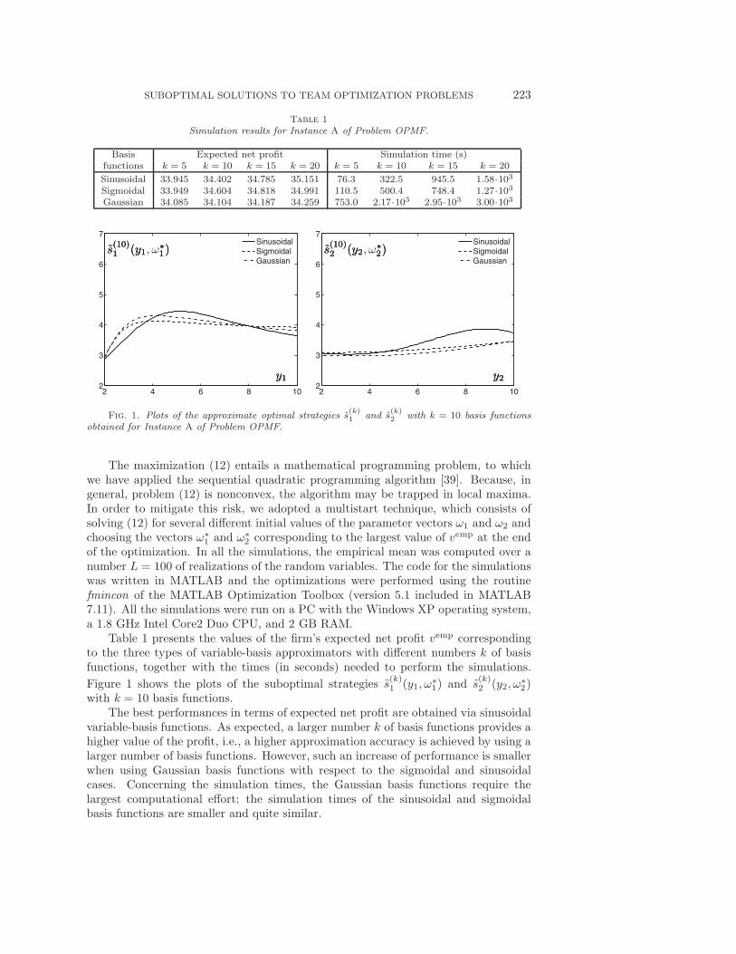
Table 1
Simulation results for Instance A of Problem OPMF.
Basis Expected net profit Simulation time (s)functions k = 5 k = 10 k = 15 k = 20 k = 5 k = 10 k = 15 k = 20
Sinusoidal 33.945 34.402 34.785 35.151 76.3 322.5 945.5 1.58·103Sigmoidal 33.949 34.604 34.818 34.991 110.5 500.4 748.4 1.27·103Gaussian 34.085 34.104 34.187 34.259 753.0 2.17·103 2.95·103 3.00·103
2 4 6 8 102
3
4
5
6
7
SinusoidalSigmoidalGaussian
s(10)1 (y1, ω
∗1)s
(10)1 (y1
∗1)s
(10)1 (y1
∗1)
y1y1y1
2 4 6 8 102
3
4
5
6
7
SinusoidalSigmoidalGaussian
s(10)2 (y2, ω
∗2)s
(10)2 (y2
∗2)s
(10)2 (y2
∗2)
y2y2y2
Fig. 1. Plots of the approximate optimal strategies s(k)1 and s
(k)2 with k = 10 basis functions
obtained for Instance A of Problem OPMF.
The maximization (12) entails a mathematical programming problem, to whichwe have applied the sequential quadratic programming algorithm [39]. Because, ingeneral, problem (12) is nonconvex, the algorithm may be trapped in local maxima.In order to mitigate this risk, we adopted a multistart technique, which consists ofsolving (12) for several different initial values of the parameter vectors ω1 and ω2 andchoosing the vectors ω∗
1 and ω∗2 corresponding to the largest value of vemp at the end
of the optimization. In all the simulations, the empirical mean was computed over anumber L = 100 of realizations of the random variables. The code for the simulationswas written in MATLAB and the optimizations were performed using the routinefmincon of the MATLAB Optimization Toolbox (version 5.1 included in MATLAB7.11). All the simulations were run on a PC with the Windows XP operating system,a 1.8 GHz Intel Core2 Duo CPU, and 2 GB RAM.
Table 1 presents the values of the firm’s expected net profit vemp correspondingto the three types of variable-basis approximators with different numbers k of basisfunctions, together with the times (in seconds) needed to perform the simulations.
Figure 1 shows the plots of the suboptimal strategies s(k)1 (y1, ω
∗1) and s
(k)2 (y2, ω
∗2)
with k = 10 basis functions.The best performances in terms of expected net profit are obtained via sinusoidal
variable-basis functions. As expected, a larger number k of basis functions provides ahigher value of the profit, i.e., a higher approximation accuracy is achieved by using alarger number of basis functions. However, such an increase of performance is smallerwhen using Gaussian basis functions with respect to the sigmoidal and sinusoidalcases. Concerning the simulation times, the Gaussian basis functions require thelargest computational effort; the simulation times of the sinusoidal and sigmoidalbasis functions are smaller and quite similar.
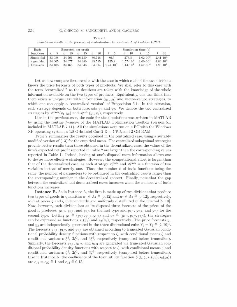
224 G. GNECCO, M. SANGUINETI, AND M. GAGGERO
Table 2
Simulation results in the presence of centralization for Instance A of Problem OPMF.
Basis Expected net profit Simulation time (s)functions k = 5 k = 10 k = 15 k = 20 k = 5 k = 10 k = 15 k = 20
Sinusoidal 33.988 34.791 36.150 36.748 86.5 273.5 1.02·103 2.41·103Sigmoidal 34.005 34.677 34.980 35.595 155.8 1.57·103 2.00·103 4.66·103Gaussian 34.108 34.468 34.846 34.914 2.44·103 1.14·104 1.67·104 1.88·104
Let us now compare these results with the case in which each of the two divisionsknows the price forecasts of both types of products. We shall refer to this case withthe term “centralized,” as the decisions are taken with the knowledge of the wholeinformation available on the two types of products. Equivalently, one can think thatthere exists a unique DM with information (y1, y2) and vector-valued strategies, towhich one can apply a “centralized version” of Proposition 5.1. In this situation,each strategy depends on both forecasts y1 and y2. We denote the two centralizedstrategies by scentr1 (y1, y2) and s
centr2 (y1, y2), respectively.
Like in the previous case, the code for the simulations was written in MATLABby using the routine fmincon of the MATLAB Optimization Toolbox (version 5.1included in MATLAB 7.11). All the simulations were run on a PC with the WindowsXP operating system, a 1.8 GHz Intel Core2 Duo CPU, and 2 GB RAM.
Table 2 summarizes the results obtained in the centralized case, using a suitablymodified version of (13) for the empirical mean. The centralized suboptimal strategiesprovide better results than those obtained in the decentralized case: the values of thefirm’s expected net profit reported in Table 2 are larger than the corresponding valuesreported in Table 1. Indeed, having at one’s disposal more information allows oneto devise more effective strategies. However, the computational effort is larger thanthat of the decentralized case, as each strategy scentr1 and scentr2 is a function of twovariables instead of merely one. Thus, the number k of basis functions being thesame, the number of parameters to be optimized in the centralized case is larger thanthe corresponding number in the decentralized context. Finally, note that the gapbetween the centralized and decentralized cases increases when the number k of basisfunctions increases.
Instance B. As in Instance A, the firm is made up of two divisions that producetwo types of goods in quantities a1 ∈ A1 � [0, 12] and a2 ∈ A2 � [0, 12], respectively,sold at prices ξ and ζ independently and uniformly distributed in the interval [2, 10].Now, however, each division has at its disposal three forecasts of the prices of thegood it produces: y1,1, y1,2, and y1,3 for the first type and y2,1, y2,2, and y2,3 for the
second type. Letting y1 � (y1,1, y1,2, y1,3) and y2 � (y2,1, y2,2, y2,3), the strategiescan be expressed as functions s1(y1) and s2(y2), respectively. The price forecasts y1and y2 are independently generated in the three-dimensional cube Y1 = Y2 � [2, 10]3.The forecasts y1,1, y1,2, and y1,3 are obtained according to truncated Gaussian condi-tional probability density functions with respect to ξ, with conditional means ξ andconditional variances ξ2, 2ξ2, and 3ξ2, respectively (computed before truncation).Similarly, the forecasts y2,1, y2,2, and y2,3 are generated via truncated Gaussian con-ditional probability density functions with respect to ζ, with conditional means ζ andconditional variances ζ2, 2ζ2, and 3ζ2, respectively (computed before truncation).Like in Instance A, the coefficients of the team utility function U(ξ, ζ, s1(y1), s2(y2))are c11 = c22 � 1 and c12 � 0.15.
SUBOPTIMAL SOLUTIONS TO TEAM OPTIMIZATION PROBLEMS 225
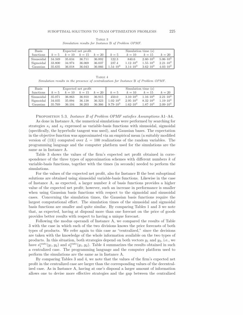
Table 3
Simulation results for Instance B of Problem OPMF.
Basis Expected net profit Simulation time (s)functions k = 5 k = 10 k = 15 k = 20 k = 5 k = 10 k = 15 k = 20
Sinusoidal 34.349 35.634 36.711 36.892 122.3 840.6 2.60·103 5.06·103Sigmoidal 33.800 34.974 36.069 36.037 237.4 1.12·103 1.55·103 2.21·103Gaussian 35.635 36.018 36.043 36.066 1.54·103 3.14·103 3.62·103 4.03·103
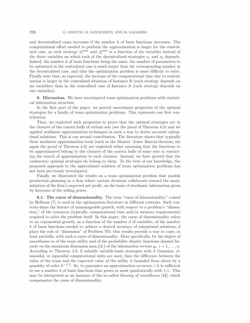
Table 4
Simulation results in the presence of centralization for Instance B of Problem OPMF.
Basis Expected net profit Simulation time (s)functions k = 5 k = 10 k = 15 k = 20 k = 5 k = 10 k = 15 k = 20
Sinusoidal 35.071 36.863 36.910 36.915 450.0 3.10·103 1.16·104 2.21·104Sigmoidal 34.035 35.094 36.138 36.323 1.02·103 2.95·103 8.32·103 1.19·104Gaussian 35.769 36.104 36.203 36.366 9.79·103 1.62·104 1.87·104 2.09·104
Proposition 5.3. Instance B of Problem OPMF satisfies Assumptions A1–A4.As done in Instance A, the numerical simulations were performed by searching for
strategies s1 and s2 expressed as variable-basis functions with sinusoidal, sigmoidal(specifically, the hyperbolic tangent was used), and Gaussian bases. The expectationin the objective function was approximated via an empirical mean (a suitably modifiedversion of (13)) computed over L = 100 realizations of the random variables. Theprogramming language and the computer platform used for the simulations are thesame as in Instance A.
Table 3 shows the values of the firm’s expected net profit obtained in corre-spondence of the three types of approximation schemes with different numbers k ofvariable-basis functions, together with the times (in seconds) needed to perform thesimulations.
For the values of the expected net profit, also for Instance B the best suboptimalsolutions are obtained using sinusoidal variable-basis functions. Likewise in the caseof Instance A, as expected, a larger number k of basis functions provides a highervalue of the expected net profit; however, such an increase in performance is smallerwhen using Gaussian basis functions with respect to the sigmoidal and sinusoidalcases. Concerning the simulation times, the Gaussian basis functions require thelargest computational effort. The simulation times of the sinusoidal and sigmoidalbasis functions are smaller and quite similar. By comparing Tables 1 and 3 we notethat, as expected, having at disposal more than one forecast on the price of goodsprovides better results with respect to having a unique forecast.
Following the modus operandi of Instance A, we compared the results of Table3 with the case in which each of the two divisions knows the price forecasts of bothtypes of products. We refer again to this case as “centralized,” since the decisionsare taken with the knowledge of the whole information available on the two types ofproducts. In this situation, both strategies depend on both vectors y1 and y2, i.e., wehave scentr1 (y1, y2) and s
centr2 (y1, y2). Table 4 summarizes the results obtained in such
a centralized case. The programming language and the computer platform used toperform the simulations are the same as in Instance A.
By comparing Tables 3 and 4, we note that the values of the firm’s expected netprofit in the centralized case are larger than the corresponding values of the decentral-ized case. As in Instance A, having at one’s disposal a larger amount of informationallows one to devise more effective strategies and the gap between the centralized
226 G. GNECCO, M. SANGUINETI, AND M. GAGGERO
and decentralized cases increases if the number k of basis functions increases. Thecomputational effort needed to perform the approximation is larger for the central-ized case, as each strategy scentr1 and scentr2 is a function of six variables instead ofthe three variables on which each of the decentralized strategies s1 and s2 depends.Indeed, the number k of basis functions being the same, the number of parameters tobe optimized in the centralized case is much larger than the corresponding number inthe decentralized case, and thus the optimization problem is more difficult to solve.Finally note that, as expected, the increase of the computational time due to central-ization is larger in the centralized situation of Instance B (each strategy depends onsix variables) than in the centralized case of Instance A (each strategy depends ontwo variables).
6. Discussion. We have investigated team optimization problems with statisti-cal information structure.
In the first part of the paper, we proved smoothness properties of the optimalstrategies for a family of team optimization problems. This represents our first con-tribution.
Then, we exploited such properties to prove that the optimal strategies are inthe closures of the convex hulls of certain sets (see the proof of Theorem 4.3) and weapplied nonlinear approximation techniques in such a way to derive accurate subop-timal solutions. This is our second contribution. The literature shows that typicallythese nonlinear approximation tools (such as the Maurey–Jones–Barron theorem; seeagain the proof of Theorem 4.3) are exploited either assuming that the functions tobe approximated belong to the closures of the convex hulls of some sets or restrict-ing the search of approximators to such closures. Instead, we have proved that the(unknown) optimal strategies do belong to them. To the best of our knowledge, theproposed approach to the approximate solution of team optimization problems hasnot been previously investigated.
Finally, we illustrated the results on a team optimization problem that modelsproduction planning in a firm where various divisions collaborate toward the maxi-mization of the firm’s expected net profit, on the basis of stochastic information givenby forecasts of the selling prices.
6.1. The curse of dimensionality. The term “curse of dimensionality,” coinedby Bellman [7], is used in the optimization literature in different contexts. Such con-texts share the feature of unmanageable growth, with respect to a problem’s “dimen-sion,” of the resources (typically, computational time and/or memory requirements)required to solve the problem itself. In this paper, the curse of dimensionality refersto an exponential growth, as a function of the number d of variables, of the numberk of basis functions needed to achieve a desired accuracy of suboptimal solutions; dplays the role of “dimension” of Problem TO. Our results provide a way to cope, atleast partially, with such a curse of dimensionality. More specifically, let the degree ofsmoothness m of the team utility and of the probability density functions depend lin-early on the maximum dimension maxi{di} of the information vectors yi, i = 1, . . . , n.According to Theorem 4.3, if suitable variable-basis strategies with k Gaussian, si-nusoidal, or sigmoidal computational units are used, then the difference between thevalue of the team and the expected value of the utility is bounded from above by aquantity of order k−1/2. So, to guarantee an approximation accuracy ε it is sufficientto use a number k of basis functions that grows at most quadratically with 1/ε. Thismay be interpreted as an instance of the so-called blessing of smoothness [42], whichcompensates the curse of dimensionality.
SUBOPTIMAL SOLUTIONS TO TEAM OPTIMIZATION PROBLEMS 227
In related studies, [43] considered three curses of dimensionality: the curses ofdimensionality in the state space, in the outcome space, and in the action space (see[43, section 1.2]). They prevent the efficient use of the classical dynamic programming(DP) algorithm [7] for the solution of dynamic optimization problems with largedimensions of the state space, and/or the outcome space, and/or the action space. Insome cases, such curses can be mitigated via the approximate dynamic programmingalgorithm described in [43], which exploits stochastic approximation methods to findapproximate solutions to the Bellman optimality equations, on which DP is based.For some classes of dynamic optimization problems, the above-mentioned blessing ofsmoothness can be exploited to mitigate the curse of dimensionality in optimal-policy-function approximation [16].
6.2. Trade-off between decentralization and smoothness. It is worth com-paring the degree of smoothness of the team utility function required to apply Theo-rem 4.3 with the degree of smoothness required to apply the same theorem in a cen-tralized context, i.e., when there is only one DM with information vector (y1, . . . , yn) ∈∏n
i=1 Yi ⊂ R
∑ni=1 di . Obviously, the value of the “one-member team” is larger than
or equal to the value of the “decentralized team” but the centralized version has atleast two drawbacks: the cost of making the whole information available to a singleDM and the larger degree m of smoothness required to apply Theorem 4.3. Indeed, inthe centralized case the degree m of smoothness has to grow linearly with respect to∑n
i=1 di, whereas in the decentralized case with n DMs the linear growth is requiredmerely with respect to max{di, i = 1, . . . , n}.
6.3. Application of quasi-Monte Carlo methods. Another interesting con-sequence of our results is the possibility for applying quasi-Monte Carlo methods [37]and related ones, such as the Korobov method (see [56] and [26, Chapter 6]), for thecomputations of the multivariable integral
v(s(k)1 , . . . , s(k)n ) = Ex,y1,...,yn
{u(x, {yi}ni=1, {s
(k)i (yi)}ni=1)
},
where s(k)1 , . . . , s
(k)n are approximations of the respective optimal strategies. Estimates
of the accuracies of such computations can be obtained via the Koksma–Hlawka in-equality [37, p. 20], which requires that the integrands have finite variation in thesense of Hardy and Krause [37, p. 19]. Considering, e.g., the case of an integrand fdefined on the r-dimensional unit-cube [0, 1]r, the formula (2.5) in [37, p. 19], which istypically used to prove that f has a finite variation in the sense of Hardy and Krause,requires that f ∈ Cr([0, 1]r), i.e., the degree of smoothness has to be at least equalto the number of variables. When m ≥
∑ni=0 di + 2 in Assumption A1, Theorem 3.2
provides such a degree of smoothness of the optimal strategies.
6.4. On the use of a greedy approximation algorithm. In deriving someof our results (in particular, Theorem 4.3), we have exploited the Maurey–Jones–Barron theorem [5, Lemma 1, p. 934] (see also [21, 41]). It allows one to deal with thecase of a utility function u(x, y1, . . . , yn, a1, . . . , an) that is separately strongly concavewith constant τ with respect to each decision variable a1, . . . , an. When the utilityis strongly concave with respect to the whole decision vector (a1, . . . , an), variable-basis suboptimal strategies with accuracies of the same order k−1/2 can be obtainedby exploiting, instead of the Maurey–Jones–Barron theorem, the greedy algorithmdeveloped in [55] to maximize strongly-concave functionals over the convex hull ofa set of basis functions. At each iteration, the algorithm proposed therein selects
228 G. GNECCO, M. SANGUINETI, AND M. GAGGERO
a suitable basis function and solves a one-dimensional mathematical programmingproblem. The application of such algorithm to Problem TO with strongly concaveutility function is made possible by the structural properties of the optimal strategies(see the proof of Theorem 4.3).
Let us consider, e.g., the proof of Theorem 4.3(i), where we have shown that eachfunction s◦i,j belongs to the closure of the convex hull of the set Gi,j(cos, di). For autility function u(x, y1, . . . , yn, a1, . . . , an) that is strongly concave with respect to the
decision vector (a1, . . . , an), the existence of a strategy s(k)i,j such that
‖s◦i,j − s(k)i,j ‖2Hi
= Eyi{|s◦i,j(yi)− s(k)i,j (yi)|2} ≤ Ci,j
k
follows by [55, Theorem IV.2]1 and the properties of the modulus of concavity of afunctional stated, e.g., in [28, Proposition 4.2(iii), (iv)] (the latter is applied to theobjective functional in Problem TO). The advantage over the proof based on theMaurey–Jones–Barron theorem is that the approach developed in [55] also provides
an algorithm (see [55, Algorithm II.1]) to find such a function s(k)i,j . The disadvantage
is that to apply the results from [55] the utility function u(x, y1, . . . , yn, a1, . . . , an) hasto be strongly concave with respect to the whole decision vector (a1, . . . , an), insteadof merely separately strongly concave with respect to each decision variable.
As the numerical results that we presented in section 5 are not the core of thepaper but are intended to demonstrate the way in which the theoretical results canbe exploited and applied to concrete situations, in the simulations we have not imple-mented [55, Algorithm II.1]. Instead, we have solved a nonlinear least squares problemvia nonlinear optimization (sequential quadratic programming) combined with a mul-tistart technique, which applies to the more general case of a utility function that isseparately strongly concave.
6.5. Application to network team optimization problems. Such problemsarise in optimization, management, and control of traffic networks. Such networksinclude, e.g., computer networks extending in large geographical areas, store-and-forward packet-switching telecommunication networks, large-scale freeway systems,reservoir networks in water-management systems, and queueing networks in manu-facturing systems. They can be modeled as graphs in which a set of nodes (withstoring capabilities) are connected through a set of links (where traffic delays andtransport costs may be incurred) that cannot be loaded with traffic above their ca-pacities. In this context, the team utility function u can be written as the sum ofa finite number of individual utility functions ui, each one associated with a singleDM (e.g., a telecommunications router) or a shared resource in the network (e.g., acommunication link). In addition, each ui depends only on a subset of the DMs [48].The DMs are the nodes of a graph, and there is an edge between two DMs iff bothappear in the same individual utility function. Traffic flows can be described by con-tinuous variables, even if the “objects” exchanged among the nodes are discrete innature (e.g., data packets, messages, cars, workpieces). This is justified whenever thenumber of objects is so large as to require macroscopic modeling. In store-and-forwardpacket-switching telecommunication networks, for instance, the DMs are the routers
1Note that [55, Theorem IV.2] refers to an optimization problem set on the convex hull of a setof functions. However, inspection of its proof shows that for a continuous objective functional [55,Theorem IV.2] can be applied to a problem formulated in the closure of the convex hull of such aset.
SUBOPTIMAL SOLUTIONS TO TEAM OPTIMIZATION PROBLEMS 229
acting as members of a team (they aim at maximizing a common objective related,e.g., to the congestions of the links). Each router has at its disposal some privateinformation (e.g., the total lengths of its incoming packet queues), on the basis ofwhich it decides how to split the incoming traffic flows into its output links.
The importance of deriving suboptimal solutions to network team optimizationproblems originates from the fact that closed-form solutions can be derived only inparticular cases (typically, under LQG hypotheses and, in the dynamic case, partiallynested information; see the introduction). The particular structure of a network teamoptimization allows for various simplifications in our model and results.
• As the strategy of each DM is influenced only by those of its neighbors in thenetwork, Assumption A3 is easier to impose.
• An extension of Theorem 3.3 to n ≥ 2 DMs can be formulated in termsof interaction terms βi,j (defined in a similar way as β1,2 in Theorem 3.3),where each (i, j) is a pair of different DMs in the team. For a network teamoptimization problem, most βi,j are expected to be equal to 0 (since theinteraction of each DM is limited to its neighbors in the graph); thereforesuch an extension takes on a simplified form.
• Since the utility function can be written as the sum of individual utilityfunctions, the integral Ex,y1,...,yn{u(x, {yi}ni=1, {si(yi)}ni=1)} � v(s1, . . . , sn)(see (2)) can be decomposed into the sum of a finite number of integrals,each typically dependent on less than
∑ni=0 di variables. So, in quasi-Monte
Carlo methods the minimum degree m of smoothness required by [37, p. 19,formula (2.5)] to prove for each integrand the finiteness of its variation in thesense of Hardy and Krause is smaller than
∑ni=0 di + 2. (Compare with the
general case discussed above.)As to specific applications to network team optimization, our smoothness results
may be applied, e.g., to stochastic versions of the congestion, routing, and band-width allocation problems considered in [32], which are stated in terms of smooth andconcave individual utility functions.
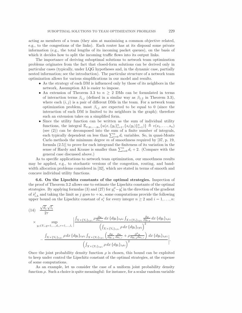
6.6. On the Lipschitz constants of the optimal strategies. Inspection ofthe proof of Theorem 3.2 allows one to estimate the Lipschitz constants of the optimalstrategies. By applying formulas (3) and (27) for y′′i −y′i in the direction of the gradient
of sji,h and taking the limit as j goes to +∞, some computations provide the followingupper bound on the Lipschitz constant of s◦i for every integer n ≥ 2 and i = 1, . . . , n:
(14)
√di
√li
2τ
× supyi∈Yi,q=1,...,di,r=1,...,li
∣∣∣∣∫X×{Yt}t�=i
ρ ∂u∂ai,r
dx {dyt}t=i
∫X×{Yt}t�=i
∂ρ∂yi,q
dx {dyt}t=i(∫X×{Yt}t�=i
ρ dx {dyt}t=i
)2
−
∫X×{Yt}t�=i
ρ dx {dyt}t=i
∫X×{Yt}t�=i
(∂ρ
∂yi,q
∂u∂ai,r
+ ρ ∂2u∂yi,q∂ai,r
)dx {dyt}t=i(∫
X×{Yt}t�=iρ dx {dyt}t=i
)2∣∣∣∣.
Once the joint probability density function ρ is chosen, this bound can be exploitedto keep under control the Lipschitz constant of the optimal strategies, at the expenseof some computations.
As an example, let us consider the case of a uniform joint probability densityfunction ρ. Such a choice is quite meaningful: for instance, for a scalar random variable

230 G. GNECCO, M. SANGUINETI, AND M. GAGGERO
it represents a situation of maximum uncertainty, in the sense that it maximizes thedifferential entropy [10] among all joint probability density functions on a compactinterval. In this case, the upper bound (14) takes on the form
(15)
√di
√li
2τsup
∣∣∣∣∂2u(x, y1, . . . , yn, a1, . . . , an)∂yi,q∂ai,r
∣∣∣∣ ,where the supremum is with respect to (x, y1, . . . , yn, a1, . . . , an) ∈ X ×
∏ni=1 Yi ×∏n
i=1 Ai , q = 1, . . . , di, and r = 1, . . . , li. So, the dependence of the Lipschitz constantof the optimal strategies on the number n of DMs can be controlled via the dependenceon n of the constant τ of separate concavity of the utility function u and the largest
absolute values of its second-order derivatives ∂2u(x,y1,...,yn,a1,...,an)∂yi,q∂ai,r
. Note that the
upper bound (15) shows the dependence on the dimensions di and li. The Lipschitzconstant does not blow up with di and li. Indeed, its rate of growth is quite slow: itis merely proportional to the product
√di
√li of the square roots of the “dimensions”
di and li of the problem. It is worth remarking that moderately large values of n andsmall values of di and li are of practical interest, as they correspond to situations inwhich one has many DMs, each with a simple structure (i.e., small dimensions of thedecision and information vectors).
A family of problems and associated utility functions u, which can be modeled inthe form of Problem TO and for which a good control of the Lipschitz constants canbe obtained, is represented by the network team optimization problems discussed insection 6.5. They share the following characteristics: (i) the strategy of each DM isinfluenced only by those of its neighbors in the network, (ii) the utility function canbe written as the sum of individual utility functions, and (iii) as the interaction ofeach DM is limited to its neighbors in the graph, each utility function depends only ona small number of DMs. Let us investigate the consequences of such features on theupper bound (15) on the Lipschitz constant and, in particular, its dependence on thenumber n of DMs. As the utility function is the sum of individual utility functions,the constant τ of separate strong concavity can be considered to be independent of n.Moreover, as each individual utility function depends only on a small number of DMs
(the neighboring ones in the graph), the term ∂2u(x,y1,...,yn,a1,...,an)∂yi,q∂ai,r
can be bounded
from above independently of n. In such a way, one can keep the Lipschitz constantsof the optimal strategies under control.
6.7. Extensions to other n-person games. Problem TO is a particular caseof n-person games (also called pure coordination games [49], a particular case of po-tential games [45]), in which the players share the same objective functional. Oursmoothness results can be extended to games in which different players may havedifferent objectives. In particular, the technique used in Step 1 of the proof of The-orem 3.2 may be applied to prove analogous smoothness properties for n-tuples ofstrategies representing a Nash equilibrium in an infinite-dimensional stochastic n-person game, like those studied in [31] and [35]. For instance, [31] provides sufficientconditions for the existence and uniqueness of a Nash equilibrium but it does notaddress the smoothness of the strategies. By our approach, one can investigate a suf-ficiently high degree of smoothness of such strategies and search for suboptimal onesimplemented by variable-basis approximation schemes with k computational units,which represent an ε-Nash equilibrium [6, section 4.2] for ε = O(1/k2) (thus withoutincurring the curse of the dimensionality). Such smoothness results may be of interestalso in the context of the so-called algorithmic game theory [38].
SUBOPTIMAL SOLUTIONS TO TEAM OPTIMIZATION PROBLEMS 231
Finally, we mention the following interpretation of our results in terms of a game:the larger the degree of smoothness of the optimal strategies, the smaller the relevanceof each component of the information vector available to each player in finding anoptimal strategy. More specifically, a small variation of such a component impliesa small variation of the optimal decision and, keeping the other factors unchanged,the dependence decreases by increasing the degree of smoothness. Roughly speaking,this property allows one to efficiently approximate the optimal strategies with a smallnumber of terms in suitable variable-basis approximation schemes.
7. Proofs. Recall that a subset F of the space C(Ω) of continuous functions onΩ ⊆ R
d is equicontinuous at z ∈ Ω iff for every ε > 0 there exists a neighborhoodU of z such that for every w ∈ U and every f ∈ F one has |f(z) − f(w)| ≤ ε.The set F is equicontinuous iff it is equicontinuous at every z ∈ Ω. The Ascoli–ArzelaTheorem [1, Theorem 1.33, p. 11] states that for a compact set Ω ⊂ R
d, a set F ⊂ C(Ω)is compact in C(Ω) iff it is closed, bounded, and equicontinuous.
Proof of Lemma 3.1. The proof proceeds as in Step 1 of the proof of [17, Theo-rem 1]; for completeness, we report it here. We give the proof for the case of n = 2DMs, then we mention the changes required for the extension to n > 2.
Proof for n = 2. Consider a sequence {sj1, sj2} of pairs of strategies, indexed by
j ∈ N+, such that
limj→∞
v(sj1, sj2) = sup
s1∈M(Y1,A1),s2∈M(Y2,A2)
v(s1, s2).
(Such a sequence exists by the definition of supremum.) From this sequence, wegenerate the sequence {sj1, s
j2} defined for every y1 ∈ Y1 and every y2 ∈ Y2 as
sj1(y1) � argmaxa1∈A1
Ex,y2 |y1{u(x, y1, y2, a1, sj2(y2))},(16)
sj2(y2) � argmaxa2∈A2
Ex,y1 |y2{u(x, y1, y2, sj1(y1), a2)}.(17)
The proof is structured as follows. First, we show that for every j ∈ N+, sj1 and
sj2 are well-defined (i.e., the maxima in (16) and (17) exist and are uniquely achieved)
and continuous, so it makes sense to evaluate v(sj1, sj2). Thus, by (2), (16), (17), and
the possibility of interchanging maximization and integration [46, Theorem 14.60], weget v(sj1, s
j2) ≥ v(sj1, s
j2). Hence,
limj→∞
v(sj1, sj2) = sup
s1∈M(Y1,A1),s2∈M(Y2,A2)
v(s1, s2).
We detail the proof for sj1; the same arguments hold for sj2.
Let us show that for every j ∈ N+ the function sj1 is well-defined and continuous.Let
M j1 (y1, a1) � Ex,y2|y1
{u(x, y1, y2, a1, sj2(y2))},
so by definition
(18) sj1(y1) = argmaxa1∈A1
M j1 (y1, a1).
As the probability density function ρ(x, y1, y2) is of class Cm and strictly positive
on X × Y1 × Y2, the conditional density ρ(x, y2|y1) = ρ(x,y1,y2)∫X×Y2
ρ(x,y1,y2)dxdy2is of class
232 G. GNECCO, M. SANGUINETI, AND M. GAGGERO
Cm on X×Y1×Y2. Let Ω be the open set containing X×Y1×Y2×A1×A2 on whichthe team utility function u is of class Cm, and for i = 1, 2, let Ai ⊃ Ai be compactand such that X × Y1 × Y2 × A1 × A2 ⊂ Ω. Since ρ(x, y2|y1) and u are of class Cm
on the compact sets X × Y1 × Y2 and X × Y1 × Y2 × A1 × A2, respectively, Mj1 is of
class Cm on the compact set Y1 × A1. (It is an integral dependent on parameters.)By [17, Lemma 1], for every y1 ∈ Y1 the function M j
1 (y1, ·) is Lipschitz and stronglyconcave with constant τ on the open set int A1 ⊃ A1, where int A1 denotes thetopological interior of A1.
By the above-proved continuity and strong concavity properties of M j1 with re-
spect to a1, for every y1 ∈ Y1 the maximum in (18) exists and is unique, so thefunction sj1(·) is well-defined. Moreover, by the necessary and sufficient optimality
condition stated in [8, Theorem 3.2, p. 138], 0 is a supergradient ofM j1 (y1, ·) for every
y1 ∈ Y1. Take y′1, y′′1 ∈ Y1. By the definition of sj1, exploiting the strong concavity
with constant τ of M j1 (y
′1, ·) and taking the supergradient 0 of M j
1 (y′1, ·) at s
j1(y
′1) we
get
(19) M j1 (y
′1, s
j1(y
′′1 ))−M j
1 (y′1, s
j1(y
′1)) ≤ −τ‖sj1(y′′1 )− sj1(y
′1)‖2.
Similarly, we obtain
(20) M j1 (y
′′1 , s
j1(y
′1))−M j
1 (y′′1 , s
j1(y
′′1 )) ≤ −τ‖sj1(y′1)− sj1(y
′′1 )‖2.
By summing (19) and (20) we have
(21) M j1 (y
′1, s
j1(y
′′1 ))−M j
1 (y′1, s
j1(y
′1)) +M j
1 (y′′1 , s
j1(y
′1))−M j
1 (y′′1 , s
j1(y
′′1 ))
≤ −2τ‖sj1(y′′1 )− sj1(y′1)‖2
and by changing the sign to both sides of (21) we have
(22) −(M j
1 (y′1, s
j1(y
′′1 ))−M j
1 (y′1, s
j1(y
′1)) +M j
1 (y′′1 , s
j1(y
′1))−M j
1 (y′′1 , s
j1(y
′′1 )))
≥ 2τ‖sj1(y′′1 )− sj1(y′1)‖2.
Together, (21) and (22) give
(23) |M j1 (y
′1, s
j1(y
′′1 ))−M j
1 (y′1, s
j1(y
′1)) +M j
1 (y′′1 , s
j1(y
′1))−M j
1 (y′′1 , s
j1(y
′′1 ))|
≥ 2τ‖sj1(y′′1 )− sj1(y′1)‖2.
Let Λj be the Lipschitz constant of the function M j1 ∈ Cm(Y1 × A1). Then
(24) |M j1 (y
′1, s
j1(y
′′1 ))−M j
1 (y′1, s
j1(y
′1)) +M j
1 (y′′1 , s
j1(y
′1))−M j
1 (y′′1 , s
j1(y
′′1 ))|
≤ |M j1 (y
′1, s
j1(y
′′1 ))−M j
1 (y′′1 , s
j1(y
′′1 ))|
+ |M j1 (y
′1, s
j1(y
′1))−M j
1 (y′′1 , s
j1(y
′1))| ≤ 2Λj‖y′′1 − y′1‖.
By (23) and (24), we obtain
2Λj‖y′′1 − y′1‖ ≥ 2τ‖sj1(y′′1 )− sj1(y′1)‖2,
i.e.,
(25) ‖sj1(y′′1 )− sj1(y′1)‖ ≤
√Λj
τ
√‖y′′1 − y′1‖,
SUBOPTIMAL SOLUTIONS TO TEAM OPTIMIZATION PROBLEMS 233
which proves the Holder continuity of sj1, hence its continuity. The continuity of sj2can be derived in the same way.
Extension to n ≥ 2. One defines the n-tuple sj1, . . . , sjn of strategies
sj1(y1) � argmaxa1∈A1
Ex,{yi}i�=1 |y1{u(x, {yi}ni=1, a1, {s
ji (yi)}ni=2)},
sj2(y2) � argmaxa2∈A2
Ex,{yi}i�=2 |y2{u(x, {yi}ni=1, s
j1(y1), a2, {s
ji (yi)}ni=3)},
...
sjn(yn) � argmaxan∈An
Ex,{yi}i�=n |yn{u(x, {yi}ni=1, {s
ji (yi)}n−1
i=1 , an)}
and applies the same arguments as in the case n = 2.Proof of Theorem 3.2. Also in this case, we detail the proof for n = 2 DMs. The
changes required for the extension to n ≥ 2 are the same as in the proof of Lemma 3.1.Consider the sequence {sj1, s
j2} of pairs of strategies, indexed by j ∈ N+, defined
in the proof of Lemma 3.1 and such that
limj→∞
v(sj1, sj2) = sup
s1∈M(Y1,A1),s2∈M(Y2,A2)
v(s1, s2).
Step 1. Let us prove that sj1 and sj2 are of class Cm−1 with upper bounds on theabsolute values of the partial derivatives (up to the order m− 1) of their components.We show also that such bounds are independent on j and y1 for sj1 and on j and y2for sj2. We make the proof for sj1; the same arguments hold for sj2.
Step 1.a. First, we prove that sj1 is of class C1 and that its Lipschitz constant is
independent of j. As Y1 is convex, it is sufficient to show that the restriction of sj1 toeach line joining every two points y′1 and y′′1 is Lipschitz with a constant that dependsneither on j nor on the line. Likewise in the proof of Lemma 3.1, let
M j1 (y1, a1) � Ex,y2|y1
{u(x, y1, y2, a1, sj2(y2))},
so by definition sj1(y1) = argmaxa1∈A1M j
1 (y1, a1). Consider the function sj1(y1(t)),
where y1(t) � y′1 + t(y′′1 − y′1) and 0 ≤ t ≤ 1. By Assumption A3 and the factthat the maximum point in (18) exists and is unique, for every 0 ≤ t ≤ 1 we get
sj1(y1(t)) ∈ intA1 = int∏li
j=1[al1,j , a
u1,j ]. Thus
(26)∂M j
1 (y1, a1)
∂a1,h
∣∣∣y1(t)=y′
1+t(y′′1 −y′
1), a1(t)=sj1(y1(t))= 0, h = 1, . . . , l1.
As M j1 (y1, ·) is of class Cm and is strongly concave with constant τ on int Ai, by (3)
we have
supa1∈int Ai
λmax(∇22,2M
j1 (y1, a1)) ≤ −2τ < 0,
where ∇22,2 denotes the Hessian with respect to the second (vector-valued) variable.
Then we can apply the vectorial form of the implicit function theorem to (26) insuch a way to study the local differentiability of the vector-valued function sj1(y1(t)).Indeed, taking the total derivative with respect to t of both sides of (26) and exploiting
234 G. GNECCO, M. SANGUINETI, AND M. GAGGERO
the fact that M j1 is of class Cm with m ≥ 2, for every h = 1, . . . , l1 we get
(27)l1∑
r=1
d1∑q=1
(∂2M j
1
∂a1,r∂a1,h
∂a1,r∂y1,q
∂y1,q∂t
+∂2M j
1
∂y1,q∂a1,h
∂y1,q∂t
)∣∣∣∣∣y1(t)=y′
1+t(y′′1 −y′
1),a1(t)=sj1(y1(t))
= 0.
Denoting by (∂2Mj
1
∂a1,r∂a1,h)−1 the elements of the negative-definite inverse of the
matrix with elements∂2Mj
1
∂a1,r∂a1,h, using (27), and renaming the indices, for every h =
1, . . . , l1 we get
da1,h(t)
dt=dsj1,h(y1(t))
dt
(28)
=
d1∑q=1
∂a1,h∂y1,q
∂y1,q∂t
∣∣∣∣∣y1(t)=y′
1+t(y′′1 −y′
1), a1(t)=sj1(y1(t))
= −l1∑
r=1
d1∑q=1
(∂2M j
1
∂a1,r∂a1,h
)−1∂2M j
1
∂y1,q∂a1,r
∂y1,q∂t
∣∣∣∣∣y1(t)=y′
1+t(y′′1 −y′
1), a1(t)=sj1(y1(t))
= −l1∑
r=1
d1∑q=1
(∂2M j
1
∂a1,r∂a1,h
)−1∂2M j
1
∂y1,q∂a1,r
∣∣∣∣∣y1(t)=y′
1+t(y′′1 −y′
1), a1(t)=sj1(y1(t))
(y′′1,q− y′1,q),
so a1(t) and sj1,h(y1) are locally differentiable. As this holds for every y1 ∈ Y1, s
j1,h(y1)
is of class C1 on the whole Y1.Since
supa1∈int Ai
|λmin|((∇22,2M
j1 (y1, a1))
−1) ≤ 1
2τ
and ‖y′′1,q − y′1,q‖ ≤ diameter (Y1), for every q and r we search for an upper bound on
| ∂2Mj1
∂y1,q∂a1,r| in (28), independent of y1 and j. By definition, we have
M j1 (y1, a1) =
∫X×Y2
ρ(x, y1, y2)u(x, y1, y2, a1, sj2(y2))dxdy2∫
X×Y2ρ(x, y1, y2)dxdy2
.
Simple calculations allow one to express∂2Mj
1
∂y1,q∂a1,ras a ratio whose numerator, for
i = 0, 1, 2 and a+ b = i, is a polynomial in
(29)
∫X×Y2
∂i[ρ(x, y1, y2)u(x, y1, y2, a1, sj2(y2))]
∂yb1,q∂aa1,r
dxdy2
and
(30)
∫X×Y2
∂iρ(x, y1, y2)
∂yb1,q∂aa1,r
dxdy2,
whereas its denominator is (∫X×Y2
ρ(x, y1, y2)dxdy2)3 ≥ δ, where δ is a positive con-
stant (hence independent of y1), whose existence and independence of y1 are guaran-teed by ρ(x, y1, y2) > 0 and the continuity of ρ(x, y1, y2) on the compact setX×Y1×Y2.
SUBOPTIMAL SOLUTIONS TO TEAM OPTIMIZATION PROBLEMS 235
Note that the change of order between expectation and up-to-second-order partialderivatives is justified by the fact that ρ(x, y1, y2) and u(x, y1, y2, a1, a2) are of class
Cm on compact sets with m ≥ 2. Then, an upper bound on | ∂2Mj1
∂y1,q∂a1,r| can be ex-
pressed in terms of the quantities
(31) supy1∈Y1
∫X×Y2
supa2∈A2
∣∣∣∣∣∂i[ρ(x, y1, y2)u(x, y1, y2, a1, a2)]
∂yb1,q∂aa1,r
∣∣∣∣∣ dxdy2
and
(32) supy1∈Y1
∫X×Y2
supa2∈A2
∣∣∣∣∣∂iρ(x, y1, y2)
∂yb1,q∂aa1,r
∣∣∣∣∣ dx dy2
related to (29) and (30), respectively, where measurability of the integrands followsby [47, Property (c), p. 38]. This bound does not depend on y1. Moreover, it does notdepend on the particular choice of sj2(y2), and therefore it is also independent of j.
Summing up, for every h = 1, . . . , l1 we have on |d sj1,h(y1(t))
d t | an upper bound
independent of y1 and j, where y1(t) � y′1 + t(y′′1 − y′1). Hence, sj1 is Lipschitz with a
constant independent of j.Step 1.b. As M j
1 is of class Cm, by taking higher-order partial derivatives of both
sides of (26) we conclude that sj1(y1) is locally of class Cm−1. As this holds for every
y1 ∈ Y1, it follows that sj1(y1) is of class Cm−1 on the whole Y1. Since M
j1 has upper
bounds on the sizes of its partial derivatives up to the order m that are independentof y1, a1, and j, then for every h = 1, . . . , l1 and every multi-index (i1, . . . , id1) such
that i1 + · · · + id1 = m − 1, for every y1 ∈ Y1 there exists on | ∂m−1 sj1,h
∂yi11,1,...,∂y
id11,d1
| a finite
upper bound that is independent of y1 and j.Step 2. By Step 1.b, for every h = 1, . . . , l1 and every multi-index (i1, . . . , id1) such
that i1 + · · ·+ id1 = m− 2, the elements of the sequence { ∂m−2 sj1,h
∂yi11,1,...,∂y
id11,d1
} of functions
are equibounded and have the same upper bound on their Lipschitz constants, so theyare equicontinuous on the compact set Y1. Hence, by the Ascoli–Arzela theorem there
exists a subsequence of { ∂m−2sj1,h
∂yi11,1,...,∂y
id11,d1
} that converges uniformly to a function defined
on Y1. Since this function is the pointwise limit of a sequences of equi-Lipschitzfunctions, it is Lipschitz with the same bound on its Lipschitz constant.
Step 3. By integratingm−2 times, we conclude that there exists a subsequence of{sj1} that converges uniformly to a strategy s◦1 ∈ Cm−2(Y1, A1) with Lipschitz (m−2)-order partial derivatives. Similarly, we can prove that there exists a subsequence of{sj2} that converges uniformly to s◦2 ∈ Cm−2(Y2, A2) with partial derivatives that areLipschitz up to the order m− 2.
Finally, by the continuity of the functional v(s1, s2) on C(Y1, A1) × C(Y2, A2)with the respective sup-norms, we obtain v(s◦1, s
◦2) = limj→∞ v(sj1, s
j2) = sups1,s2
v(s1, s2).
236 G. GNECCO, M. SANGUINETI, AND M. GAGGERO
Proof of Theorem 3.3. Inspection of the proof of Lemma 3.1 shows that there existsa (possibly nonlinear) operator T : C(Y1, A1)×C(Y2, A2) → C(Y1, A1)×C(Y2, A2) suchthat
T1(s1, s2) = argmaxs1∈C(Y1,A1)
v(s1, s2),
T2(s1, s2) = argmaxs2∈C(Y2,A2)
v(T1(s1, s2), s2).
Moreover, it also shows that
T1(s1, s2)(y1) = argmaxa1
Ex,y2 |y1{u(x, y1, y2, a1, s2(y2))} ∀y1 ∈ Y1,
T2(s1, s2)(y2) = argmaxa2
Ex,y1 |y2{u(x, y1, y2, T1(s1, s2)(y1), a2)} ∀y2 ∈ Y2.
Suppose by contradiction that there exist another optimal pair (s◦′
1 , s◦′2 ) ∈ C(Y1, A1)×
C(Y2, A2) of strategies. Then (s◦′
1 , s◦′2 ) = T (s◦
′1 , s
◦′2 ) is a necessary condition for its
optimality. (Otherwise there would exist a strictly better pair of strategies by an ap-plication of the theorem on interchange of maximization and integration [46, Theorem14.60].) Moreover, by the proof of Lemma 3.1 and the compactness of Y1 and Y2, forevery (s1, s2) ∈ C(Y1, A1) × C(Y2, A2) the strategies T1(s1, s2) and T2(s1, s2) belongto the interiors (with respect to the associated sup-norms) of C(Y1, A1) and C(Y2, A2)as subsets of C(Y1,Rl1) and C(Y2,Rl2), respectively, so Problem TO is reduced to anunconstrained infinite-dimensional optimization problem on C(Y2,Rl2)× C(Y2,Rl2).
Now, we reduce Problem TO to an unconstrained infinite-dimensional game-theory problem on a Hilbert space, to which one can apply the techniques developedin [31] to investigate the stability of Nash equilibria. This can be done since everypair of optimal strategies for Problem TO represents a Nash equilibrium for a two-player game, for which the individual utilities are the same and equal to v(s1, s2). Tothis end, we first endow C(Y1,Rl1) and C(Y2,Rl2) with the norms
√Ey1{‖s1(y1)‖2}
and√Ey2{‖s2(y2)‖2}, respectively; then we extend by density such spaces to the
Lebesgue spaces L2(Y1, ρy1 ,Rl1) and L2(Y2, ρy2 ,R
l2), respectively, where ρy1 and ρy2
are the marginal densities of y1 and y2. Note that thanks to the choice of a team util-ity function that is quadratic with respect to a1 and a2, by removing the constraintsa1 ∈ A1 and a2 ∈ A2 the definition of the functional v(s1, s2) can be extended on thespace L2(Y1, ρy1 ,R
l1) × L2(Y2, ρ2,Rl2). Moreover, definition (33) of the operator T
can be extended on L2(Y1, ρy1 ,Rl1)× L2(Y2, ρ2,R
l2) by setting
T1(s1, s2) � argmaxs1∈L2(Y1,ρy1 ,R
l1)
v(s1, s2),
T2(s1, s2) � argmaxs2∈L2(Y2,ρy2 ,R
l2)
v(T1(s1, s2), s2).(33)
Indeed, nonemptyness of the sets argmax in (33) follows by the direct method of thecalculus of variations [12] by standard coercivity and upper-semicontinuity arguments.The fact that they are singletons follows by strict concavity arguments.
Proceeding as in [23, Chapter XVII, section 3], we get the following expressionsfor the Frechet differentials of the integral functional v up to the second order (we
SUBOPTIMAL SOLUTIONS TO TEAM OPTIMIZATION PROBLEMS 237
denote by hi and h′i the independent increments of si, i = 1, 2):
Ds1v(s1, s2){h1} = Ex,y1,y2{h1(y1)T∇4u(x, y1, y2, s1(y1), s2(y2))}� Ey1{h1(y1)T (∇s1v(s1, s2))(y1)},
Ds2v(s1, s2){h2} = Ex,y1,y2{h2(y2)T∇5u(x, y1, y2, s1(y1), s2(y2))}� Ey2{h2(y2)T (∇s2v(s1, s2))(y2)},
D2s1,s1v(s1, s2){h1, h
′1} = Ex,y1,y2{h1(y1)T∇2
4,4u(x, y1, y2, s1(y1), s2(y2))h′1(y1)}
� Ey1{h1(y1)T (∇2s1,s1v(s1, s2)h
′1)(y1)},
D2s1,s2v(s1, s2){h1, h2} = Ex,y1,y2{h1(y1)T∇2
4,5u(x, y1, y2, s1(y1), s2(y2))h2(y2)}� Ey1{h1(y1)T (∇2
s1,s2v(s1, s2)h2)(y1)},(34)
D2s2,s1v(s1, s2){h2, h1} = Ex,y1,y2{h2(y2)T∇2
5,4u(x, y1, y2, s1(y1), s2(y2))h1(y1)}� Ey2{h2(y2)T (∇2
s2,s1v(s1, s2)h1)(y2)},(35)
D2s2,s2v(s1, s2){h2, h
′2} = Ex,y1,y2{h2(y2)T∇2
5,5u(x, y1, y2, s1(y1), s2(y2))h′2(y2)}
� Ey2{h2(y2)T (∇2s2,s2v(s1, s2)h
′2)(y2)},
where, for every j, k = 1, 2, the symbols Dsj and Dsj ,sk denote Frechet derivatives,∇sjv(s1, s2) is a function in L2(Yj , ρj ,R
lj ), and ∇sj ,skv(s1, s2) is a bounded linear op-erator from L2(Yk, ρk,R
lk) to L2(Yj , ρj ,Rlj ). In particular, it follows by Assumption
A2 that
Ex,y1,y2{h1(y1)T∇24,4u(x, y1, y2, s1(y1), s2(y2))h1(y1)} ≤ −2τEy1{‖h1(y1)‖2}
and
Ex,y1,y2{h2(y1)T∇25,5u(x, y1, y2, s1(y1), s2(y2))h2(y2)} ≤ −2τEy2{‖h2(y2)‖2}.
Then for every j = 1, 2, by the expression of such an operator ∇sj ,sjv(s1, s2) (or by anapplication of the Lax–Milgram theorem [2, p. 69]) it follows that (∇2
sj ,sjv(s1, s2))−1
exists, it is a bounded operator, and ‖(∇2sj ,sjv(s1, s2))
−1‖ ≤ 12τ . By exploiting (34)
and (35), as the second-order terms ∇24,5u(x, y1, y2, s1(y1), s2(y2)) and ∇2
5,4u(x, y1, y2,s1(y1), s2(y2)) do not depend on s1(y1) and s2(y2) we get
‖∇2s1,s2v(s1, s2)‖ = ‖∇2
s2,s1v(s1, s2)‖ ≤ β1,2
�√d1√d2 max
(x,y1,y2)∈X×Y1×Y2
maxq=1,...,l1, r=1,...,l2
∣∣∣∣ ∂2
∂a1,q∂a2,ru(x, y1, y2, a1, a2)
∣∣∣∣.(36)
Then, by applying [31, Theorem 1, formula (1)], it follows that T is a contractionoperator on L2(Y1, ρ1,R
l1)×L2(Y2, ρ2,Rl2) with a contraction constant bounded from
above byβ21,2
4τ2 < 1. Hence T has a unique fixed point (s◦′
1 , s◦′2 ), which necessarily
238 G. GNECCO, M. SANGUINETI, AND M. GAGGERO
coincides with (s◦1, s◦2). (It is also a fixed point of T and belongs to Cm−2(Y1, A1) ×
Cm−2(Y2, A2).)Proof of Theorem 3.4. Suppose by contradiction that there exists another optimal
n-tuple (s◦′
1 , . . . , s◦′n ) ∈ C(Y1, A1) × · · · × C(Yn, An) of strategies. For λ ∈ (0, 1), let
(s′1, . . . , s′n) � λ(s◦1, . . . , s
◦n) + (1− λ)(s◦
′1 , . . . , s
◦′n ). (Note that this is an admissible n-
tuple of strategies, as s′i : Yi → Ai.) By the strict concavity of the team utility function
u with respect to (a1, . . . , an) and the fact that the n-tuples (s◦′
1 (y1), . . . , s◦′n (yn)) and
(s◦1(y1), . . . , s◦n(yn)) differ on a set of (strictly) positive measure, we have
Ex,y1,...,yn {u(x, {yi}ni=1, {s′i(yi)}ni=1)}> λEx,y1,...,yn {u(x, {yi}ni=1, {s◦i (yi)}ni=1)}
+ (1− λ)Ex,y1,...,yn
{u(x, {yi}ni=1, {s◦
′i (yi)}ni=1)
}= sup
{v(s1, . . . , sn) |si∈C(Yi, Ai), i=1, . . . , n
},
which contradicts the optimality of (s◦′
1 , . . . , s◦′n ). Thus, (s◦1, . . . , s◦n) is the unique
optimal n-tuple of strategies in C(Y1, A1)×· · ·×C(Yn, An) (and also in Cm−2(Y1, A1)×· · · × Cm−2(Yn, An)).
Proof of Theorem 4.1. Let us consider n = 2 DMs. The general case can beproved similarly. For an integrable real-valued random variable z and a measurableconcave function f , the Jensen inequality [47, Theorem 3.3, p. 62] gives
(37) f (Ez{z}) ≥ Ez {f(z)} .
By the existence of an optimal solution, the Lipschitz continuity of the team utilityfunction u, and (37) we get
v(s◦1, s◦2)− v(s1, s2) = Ex,y1,y2{u(x, y1, y2, s◦1(y1), s◦2(y2)) − u(x, y1, y2, s1(y1), s2(y2))}
≤ L · Ex,y1,y2
{√‖s◦1(y1)− s1(y1)‖2 + ‖s◦2(y2)− s2(y2)‖2
}
≤ L · Ex,y1,y2
{√‖s◦1(y1)− s1(y1)‖2 +
√‖s◦2(y2)− s2(y2)‖2
}
≤ L ·([
Ey1{‖s◦1(y1)− s1(y1)‖2}]1/2
+[Ey2{‖s◦2(y2)− s2(y2)‖2}
]1/2).
Proof of Theorem 4.2. Proceeding as in the proof of Theorem 3.3, Problem TO isreduced to an unconstrained infinite-dimensional optimization problem on C(Y1, A1)×· · ·×C(Yn, An), where each space C(Yi,Rli) ⊃ C(Yi, Ai) is endowed with the respectivesup-norm, i = 1, . . . , n. By the necessary first-order optimality condition, the first-order Frechet derivatives of the integral functional v computed at (s◦1, . . . , s
◦n) are
equal to 0. So, by exploiting the concavity of the functional v (which follows by theassumptions on u) and the Taylor theorem with Lagrange’s remainder, we get
(38) v(s1, . . . , sn)− v(s◦1, . . . , s◦n) =
1
2D2v(χ){h, h},
where h = (s1 − s◦1, . . . , sn − s◦n), (s1, . . . , sn) is any other n-tuple of admissible con-tinuous strategies, and χ � (χ1, . . . , χn) belongs to the segment between (s1, . . . , sn)and the optimal solution (s◦1, . . . , s
◦n).
SUBOPTIMAL SOLUTIONS TO TEAM OPTIMIZATION PROBLEMS 239
As by assumption m ≥ 3, proceeding as in [23, Chapter XVII, section 3], thesecond-order Frechet differential D2v(χ){h, h} has the expression
Ex,y1,...,yn{(h1(y1), . . . ,hn(yn))T∇2(n+2,...,2n+1),(n+2,...,2n+1)
u(x, y1, . . . , yn, χ1(y1), . . . , χn(yn))(h1(y1), . . . , hn(yn))},
which by (3) is bounded from above by
−2τ Ex,y1,...,yn{‖(h1(y1), . . . , hn(yn))‖2} = −2τ
n∑i=1
Eyi{‖s◦i (yi)− si(yi)‖2}.
The statement follows by this last bound and (38).For Ω ⊆ R
d and 1 ≤ p < ∞, we denote the corresponding Lebesgue spaceand norm by Lp(Ω) and ‖ · ‖Lp(Ω), respectively. For Ω open, a positive integer mand 1 ≤ p < ∞, we denote by Wm,p(Ω) the Sobolev space of functions whose weakpartial derivatives up to the order m are in Lp(Ω). By C∞(Ω) we denote the space offunctions on Ω that are continuous together with their partial derivatives up to everyorder; C0(Ω) and C∞
0 (Ω) are the spaces of functions in C(Ω) and C∞(Ω), respectively,with compact supports in Ω [1, p. 2]. We denote by Wm,p
0 (Ω) the closure of C∞0 (Ω)
in the Sobolev space Wm,p(Ω) (see [1, p. 59]). For α > 0, the Bessel potential oforder α on R
d, denoted by Bα(x), is the inverse Fourier transform of the function
Bα(ω) � (2π)−d2 (1 + ‖ω‖2)−α/2. When α > d, the function Bα is continuous [51,
p. 132]. For α > 0 and 1 ≤ p < ∞, Bαp (R
d) is the Bessel potential space, whose
elements are functions u such that u = f ∗ Bα, where f ∈ Lp(Rd) [51, p. 134].
For completeness, we report the statement of [15, Corollary 5.2], as we shallexploit it in the proof of Theorem 4.3(ii).
Theorem 7.1 (see [15, Corollary 5.2]). Let d be a positive integer and α > d. Forevery f ∈ Bα
1 (Rd) and every positive integer k, there exist t1, . . . , tk ∈ R
d, b1, . . . , bk >0, c1, . . . , ck ∈ {−1,+1}, and an absolute positive constant C such that
supx∈Rd
∣∣∣∣∣f(x)− K(α, d)
k
k∑i=1
ci e− ‖x−ti‖2
bi
∣∣∣∣∣ ≤ C K(α, d)
√d+ 3
k,
where K(α, d) � 2−d/2 Γ(α/2−d/2)Γ(α/2) ‖λ‖L1(Rd) and Γ(z) �
∫∞0 sz−1e−s ds is the Gamma
function.
Proof of Theorem 4.3. (i), first case: s(k)i ∈ S
(k)i (cos, di). By Theorem 3.2,
there exist optimal strategies s◦i : Yi → Ai such that for j = 1, . . . , li, s◦i,j is of
class Cm−2 and has partial derivatives that are Lipschitz up to the order m − 2, sos◦i,j ∈ Wm−1,∞(int(Yi)).
Since Yi is bounded, s◦i,j ∈ Wm−1,∞(int(Yi)) implies s◦i,j ∈ Wm−1,p(int(Yi)) forevery 1 ≤ p < ∞. As every Yi is a bounded convex set, by the Sobolev extensiontheorem (see [51, Theorem 5, p. 181] and [51, Example 2, p. 189]), s◦i,j can then be
extended to a function s◦,ext,pi,j ∈ Wm−1,p(Rdi).
Let Y ′i � (yli,1, y
ui,1)× · · · × (yli,di
, yui,di) ⊃ Yi and consider a function ψi ∈ C∞
0 (Y ′i )
such that ψi(yi) = 1 for every yi ∈ Yi. By an application of [1, Theorem 3.22,p. 68], s◦,′,pi,j � s◦,ext,pi,j · ψi ∈ Wm−1,p
0 (Y ′i ) if 1 ≤ p < ∞. By the Sobolev embedding
theorem [1, Theorem 4.12, p. 85], if di < p <∞, thenWm−1,p0 (Y ′
i ) ⊂ Cm−2([yli,1, yui,1]×
· · · × [yli,di, yui,di
]).
240 G. GNECCO, M. SANGUINETI, AND M. GAGGERO
From now on, we assume di < p < ∞. Let {Si,j,r1,...,rdi} be the set of the
coefficients of the Fourier series expansion of s◦,ext,pi,j on Y ′i . Note that by construction,
the periodic extension of s◦,′,pi,j on Rdi is of class Cm−2(Rdi). We apply a particular
case of an extension to multiple Fourier series [18, p. 647] of the Bernstein theoremin Fourier analysis, according to which the condition m− 2 > di
2 implies
Ki,j �∞∑
r1,...,rdi=0
|Si,j,r1,...,rdi| <∞.
Thus, s◦,′,pi,j belongs to the closure (with respect to the L2(Y′i )-norm) of the convex
hull of the set
G′i,j(cos, di) �
{gi : Y
′i → R
∣∣∣ gi(yi) = b
di∏r=1
cos(ωi,ryi,r + θi,r),
|b| ≤ Ki,j, ωi,r =2πh
yui,r − yli,r, h ∈ N, θi,r ∈ [0, 2π)
}.
Let Hi be the Hilbert space of functions fi : Yi → R such that Eyi{|fi(yi)|2} < ∞,where the expected value is evaluated on Yi with the marginal probability densityfunction ρyi induced by ρ. As the probability density function ρ is bounded, s◦i,jbelongs to the closure (with respect to the norm of Hi) of the convex hull of the set
Gi,j(cos, di) �{gi : Yi → R
∣∣∣ gi(yi) = b
di∏r=1
cos(ωi,ryi,r + θi,r),
|b| ≤ Ki,j, ωi,r =2πh
yui,r − yli,r, h ∈ N, θi,r ∈ [0, 2π)
}.(39)
Moreover, for every gi ∈ Gi,j(cos, di) ⊂ Gi(cos, di) we have
‖gi‖Hi =√Eyi{|gi(yi)|2} ≤ Ki,j.
Hence, by the Maurey–Jones–Barron theorem [5, Lemma 1, p. 934] (see also [21, 41]),for every positive integer k ≥ 1 and every Ci,j > K2
i,j−‖s◦i,j‖2Hithere exists a function
s(k)i,j in the convex hull of k elements of Gi,j(cos, di) such that
(40) ‖s◦i,j − s(k)i,j ‖2Hi
= Eyi
{∣∣∣s◦i,j(yi)− s(k)i,j (yi)
∣∣∣2} ≤ Ci,j
k.
We conclude the proof by taking projections on Ai,j and applying (40) and Theo-rem 4.1.
(i), second case: s(k)i ∈ S
(k)i (σ, di). As in the proof of the first case, by choosing p =
2 the function s◦i,j can be extended to s◦,ext,2i,j ∈ Wm−1,2(Rdi). Let s◦,ext,2i,j be its Fourier
transform. By similar arguments as in [5, Example 15, p. 941] (based on the Cauchy–Schwarz inequality), the condition m−1 > di/2+1 implies
∫Rdi
|s◦,ext,2i,j (ω)|‖ω‖2 dω <+ ∞. So one can apply [5, Theorem 1] to s◦i,j on Yi, thus obtaining for sigmoidalcomputational units the same approximation error bound as in (40), in general with
SUBOPTIMAL SOLUTIONS TO TEAM OPTIMIZATION PROBLEMS 241
different constants Ci,j . We conclude by taking projections onto Ai,j and applyingsuch a bound and Theorem 4.1.
(ii) As in the proof of item (i), by choosing p = 1 the function s◦i,j can be ex-
tended to s◦,ext,1i,j ∈ Wm−1,1(Rdi). As m − 1 is even, we can exploit the inclusionof Sobolev spaces into Bessel potential spaces stated in [51, Remark 6.6 (b), p. 160].Then, there exists λi,j ∈ L1(R
di) such that s◦,ext,1i,j = Bm−1 ∗ λi,j . Since m − 1 > diwe can apply [15, Corollary 5.2], reported above as Theorem 7.1. This, together withthe fact that the L2-norm of a function defined on the bounded domain Yi can bebounded from above by a constant times its sup-norm, provides for the case of Gaus-sian computational units the same approximation error bound as in (40), in generalwith different constants Ci,j . As before, we conclude the proof by taking projectionsonto Ai,j and applying such an error bound and Theorem 4.1.
Proof of Proposition 5.1. The statement follows by Theorems 3.2 and 4.3.Proof of Proposition 5.2. The joint probability density function ρ(ξ, ζ, y1, y2) can
be written as
ρ(ξ, ζ, y1, y2) = ρ(ξ, y1)ρ(ζ, y2) = ρ(y1|ξ)ρ(ξ)ρ(y2|ζ)ρ(ζ)
=(2πξ2)−1/2 e−(y1−ξ)2/(2ξ2)
(2πξ2)−1/2∫ 10
2e−(y1−ξ)2/(2ξ2) dy1
· 18
· (2πζ2)−1/2 e−(y2−ζ)2/(2ζ2)
(2πζ2)−1/2∫ 10
2e−(y2−ζ)2/(2ζ2) dy2
· 18.
This function is positive on [ξmin, ξmax]× [ζmin, ζmax] × Y1 × Y2 and for every m ≥ 2enjoys the properties required in Assumption A1.
As the team utility function u has only linear and quadratic terms, AssumptionA2 is satisfied by taking τ � 1
2 min{c11, c22} = 12 > 0.
Assumption A3 can be verified as follows (recall that intA1 denotes the topologicalinterior of A1). For every y1 ∈ Y1 and every admissible strategy s2, the function
M1(y1, a1) � Ex,y2|y1
{ξa1 + ζs2(y2)−
1
2c11a
21 − c12a1s2(y2)−
1
2c22s2(y2)
2
}
is strictly concave and differentiable, and argmaxa1∈A1M1(y1, a1) ∈ intA1 iff for some
a∗1 ∈ intA1 one has
∂
∂a1M1(y1, a1)
∣∣∣a1=a∗
1
= Eξ|y1{ξ} − c11a
∗1 − c12Ey2|y1
{s2(y2)} = 0.
Note that a∗1 � Eξ|y1{ξ}−c12Ey2|y1{s2(y2)}c11
∈ intA1, as
2− 0.15 · 10 = 0.5 ≤Eξ|y1
{ξ} − c12Ey2|y1{s2(y2)}
c11≤ 10− 0.15 · 2 = 9.7
and [0.5, 9.7] ⊂ intA1. Similar arguments hold for every admissible strategy of theother DM, so we conclude that Assumption A3 is satisfied.
Finally, Assumption A4 holds since the sets A1 and A2 are closed and boundednonempty intervals.
Proof of Proposition 5.3. The proof exploits the same arguments as those in theproof of Proposition 5.2.
242 G. GNECCO, M. SANGUINETI, AND M. GAGGERO
REFERENCES
[1] R. A. Adams and J. J. F. Fournier, Sobolev Spaces, Academic Press, Amsterdam, 2003.[2] H. Attouch, G. Buttazzo, and G. Michaille, Variational Analysis in Sobolev and BV
Spaces: Applications to PDEs and Optimization, SIAM, Philadephia, 2005.[3] Y. Azrieli and E. Lehrer, The value of a stochastic information structure, Games Econom.
Behav., 63 (2008), pp. 679–693.[4] T. Basar and R. Bansal, The Theory of Teams: A Selective Annotated Bibliography, Lecture
Notes in Control and Inform. Sci. 119, Springer, Berlin, 1989.[5] A. R. Barron, Universal approximation bounds for superpositions of a sigmoidal function,
IEEE Trans. Inform. Theory, 39 (1993), pp. 930–945.[6] T. Basar and G. J. Olsder, Dynamic Noncooperative Game Theory, 2nd ed., SIAM, Philadel-
phia, 1999.[7] R. Bellman, Dynamic Programming, Princeton University Press, Princeton, NJ, 1957.[8] L. D. Berkovitz, Convexity and Optimization in Rn, Wiley, New York, 2002.[9] T. W. S. Chow and S.-Y. Cho, Neural Networks and Computing: Learning Algorithms and
Applications, World Scientific, River Edge, NJ, 2007.[10] T. M. Cover and J. A. Thomas, Elements of Information Theory, Wiley, New York, 2006.[11] G. Cybenko, Approximation by superpositions of a sigmoidal function, Math. Control Signals
Systems, 2 (1989), pp. 303–314.[12] B. Dacorogna, Introduction to the Calculus of Variations, Imperial College Press, London,
2004.[13] S. Giulini and M. Sanguineti, On dimension–independent approximation by neural networks
and linear approximators, in Proceedings of the International Joint Conference on NeuralNetworks, 2000, pp. I283–I288.
[14] S. Giulini and M. Sanguineti, Approximation schemes for functional optimization problems,J. Optim. Theory Appl., 140 (2009), pp. 33–54.
[15] G. Gnecco and M. Sanguineti, Approximation error bounds via Rademacher’s complexity,Appl. Math. Sci., 2 (2008), pp. 153–176.
[16] G. Gnecco and M. Sanguineti, Suboptimal solutions to dynamic optimization problems viaapproximations of the policy functions, J. Optim. Theory Appl., 146 (2010), pp. 764–794.
[17] G. Gnecco and M. Sanguineti, Team optimization problems with Lipschitz continuous strate-gies, Optim. Lett., 5 (2011), pp. 333–346.
[18] B. I. Golubov, Multiple Fourier series and integrals, J. Math. Sci., 24 (1984), pp. 639–673.[19] J. Hess, Z. Ider, H. Kagiwada, and R. Kalaba, Team decision theory and integral equations,
J. Optim. Theory Appl., 22 (1977), pp. 251–264.[20] Y.-C. Ho and K.-C. Chu, Team decision theory and information structures in optimal control
Part I, IEEE Trans. Automat. Control, 17 (1972), pp. 15–22.[21] L. K. Jones, Constructive approximation for neural networks by sigmoid functions, Proc.
IEEE, 78 (1990), pp. 1586–1589.[22] P. C. Kainen, V. Kurkova, and M. Sanguineti, Dependence of computational models on in-
put dimension: Tractability of approximation and optimization tasks, IEEE Trans. Inform.Theory, 58 (2012), pp. 1203–1214.
[23] L. Kantorovich and G. Akilov, Functional Analysis in Normed Spaces, Pergamon Press,Oxford, UK, 1964.
[24] K. H. Kim and F. W. Roush, Team Theory, Ellis Horwood Limited, Chichester, UK, 1987.[25] J. C. Krainak, J. L. Speyer, and S. I. Marcus, Static team problems Part I: Sufficient
conditions and the exponential cost criterion, IEEE Trans. Authomat. Control, 27 (1982),pp. 839–848.
[26] A. R. Krommer and C. W. Ueberhuber, Computational Integration, SIAM, Philadelphia,1998.
[27] V. Kurkova and M. Sanguineti, Comparison of worst case errors in linear and neural net-work approximation, IEEE Trans. Inform. Theory, 48 (2002), pp. 264–275.
[28] V. Kurkova and M. Sanguineti, Error estimates for approximate optimization by the ex-tended Ritz method, SIAM J. Optim., 18 (2005), pp. 461–487.
[29] V. Kurkova and M. Sanguineti, Approximate minimization of the regularized expected errorover kernel models, Math. Oper. Res., 33 (2008), pp. 747–756.
[30] V. Kurkova and M. Sanguineti, Geometric upper bounds on rates of variable-basis approxi-mation, IEEE Trans. Inform. Theory, 54 (2008), pp. 5681–5688.
[31] S. Li and T. Basar, Distributed algorithms for the computation of noncooperative equilibria,Automatica, 23 (1987), pp. 523–533.
[32] Y. Mansour, Lecture Notes for a Course on Computational Game Theory, http://www.cs.tau.ac.il/˜mansour/course games/2006/course games 05 06.htm (2006).
SUBOPTIMAL SOLUTIONS TO TEAM OPTIMIZATION PROBLEMS 243
[33] J. Marschak, Elements for a theory of teams, Manage. Sci., 1 (1955), pp. 127–137.[34] J. Marschak and R. Radner, Economic Theory of Teams, Yale University Press, New Haven,
CT, 1972.[35] P. Milgrom and R. J. Weber, Distributional strategies for games with incomplete informa-
tion, Math. Oper. Res., 10 (1985), pp. 619–632.[36] L. Montrucchio, Lipschitz continuous policy functions for strongly concave optimization prob-
lems, J. Math. Econom., 16 (1987), pp. 259–273.[37] H. Niederreiter, Random Number Generation and Quasi-Monte Carlo Methods, SIAM,
Philadelphia, 1992.[38] N. Nisan, T. Roughgarden, E. Tardos, and V. V. Vazirani, Algorithmic Game Theory,
Cambridge University Press, Cambridge, UK, 2007.[39] J. Nocedal and S. J. Wright, Numerical Optimization, Springer, New York, 2006.[40] C. H. Papadimitriou and J. N. Tsitsiklis, Intractable problems in control theory, SIAM J.
Control Optim., 24 (1986), pp. 639–654.[41] G. Pisier, Remarques sur un resultat non publie de B. Maurey, in Seminaire d’Analyse Fonc-
tionnelle 1980-81, vol. I, no. 12, Ecole Polytechnique, Centre de Mathematiques, Palaiseau,France, 1981.
[42] T. Poggio and S. Smale, The mathematics of learning: Dealing with data, Not. Amer. Math.Soc., 50 (2003), pp. 537–544.
[43] W. B. Powell, Approximate Dynamic Programming: Solving the Curses of Dimensionality,Wiley, Hoboken, NJ, 2007.
[44] R. Radner, Team decision problems, Ann. Math. Statist., 33 (1962), pp. 857–881.[45] A. Rantzer, Using Game Theory for Distributed Control Engineering, Technical report ISRN
LUTFD2/TFRT–7620–SE, Lund University, Sweden, 2008.[46] R. T. Rockafellar and R. J.-B. Wets, Variational Analysis, Springer, Berlin, 2004.[47] W. Rudin, Real and Complex Analysis, McGraw-Hill, Singapore, 1987.[48] P. Rusmevichientong and B. Van Roy, Decentralized decision-making in a large team with
local information, Games Econom. Behav., 43 (2003), pp. 266–295.[49] Y. Shoham and K. Leyton-Brown, Multiagent Systems: Algorithmic, Game-Theoretic, and
Logical Foundations, Cambridge University Press, Cambridge, UK, 2009.[50] I. Singer, Best Approximation in Normed Linear Spaces by Elements of Linear Subspaces,
Springer, Berlin, 1970.[51] E. M. Stein, Singular Integrals and Differentiability Properties of Functions, Princeton Uni-
versity Press, Princeton, NJ, 1970.[52] J. N. Tsitsiklis and M. Athans, On the complexity of decentralized decision making and
detection problems, IEEE Trans. Automat. Control, 30 (1985), pp. 440–446.[53] H. S. Witsenhausen, Equivalent stochastic control problems, Math. Control Signals Systems,
1 (1988), pp. 3–11.[54] Y. Xu, Lecture notes on orthogonal polynomials of several variables, in Advances in the Theory
of Special Functions and Orthogonal Polynomials, W. zu Castell, F. Filbir, and B. Forster,eds., Nova Science Publishers, Hauppauge, NY, 2004, pp. 135–188.
[55] T. Zhang, Sequential greedy approximation for certain convex optimization problems, IEEETrans. Inform. Theory, 49 (2003), pp. 682–691.
[56] T. Zinterhof, High dimensional integration: New weapons fighting the curse of dimensional-ity, Phys. Part. Nuclei, 5 (2008), pp. 145–149.
[57] T. Zolezzi, Condition numbers and Ritz type methods in unconstrained optimization, Controland Cybernet., 36 (2007), pp. 811–822.
[58] R. Zoppoli, M. Sanguineti, and T. Parisini, Approximating networks and extended Ritzmethod for the solution of functional optimization problems, J. Optim. Theory Appl., 112(2002), pp. 403–439.