Embed Size (px)
Citation preview

A FINITE ELEMENT MODEL FOR THE INVESTIGATION
OF SURFACE EMG SIGNALS DURING DYNAMIC
CONTRACTION
by
Michelle Joubert
Submitted in partial fulfilment of the requirements for the degree
Master of Engineering (Bio-Engineering)
in the
Faculty of Engineering, the Built Environment and Information Technology
UNIVERSITY OF PRETORIA
September 2007

Electrical, Electronic and Computer Engineering i
Summary
Title: A finite element model for the investigation of surface EMG signals
during dynamic contraction
Author: Michelle Joubert
Supervisor: Prof. T. Hanekom
Co-supervisor: Prof. Dr. D. Farina
Department: Electrical, Electronic and Computer Engineering
Degree: Master of Engineering (Bio-Engineering)
A finite element (FE) model for the generation of single fiber action potentials (SFAPs) in
a muscle undergoing various degrees of fiber shortening has been developed. The muscle
is assumed to be fusiform with muscle fibers following a curvilinear path described by a
Gaussian function. Different degrees of fiber shortening are simulated by changing the
parameters of the fiber path and maintaining the volume of the muscle constant. The
conductivity tensor is adapted to the muscle fiber orientation. At each point of the volume
conductor, the conductivity of the muscle tissue in the direction of the fiber is larger than
that in the transversal direction. Thus, the conductivity tensor changes point-by-point with
fiber shortening, adapting to the fiber paths. An analytical derivation of the conductivity
tensor is provided. The volume conductor is then studied with an FE approach using the
analytically derived conductivity tensor (Mesin, Joubert, Hanekom, Merletti & Farina
2006).
Representative simulations of SFAPs with the muscle at different degrees of shortening are
presented. It is shown that the geometrical changes in the muscle, which imply changes in
the conductivity tensor, determine important variations in action potential shape, thus
affecting its amplitude and frequency content.
The model is expanded to include the simulation of motor unit action potentials (MUAPs).
Expanding the model was done by assigning each single fiber (SF) in the motor unit (MU)
a random starting position chosen from a normal distribution. For the model 300 SFs are

Electrical, Electronic and Computer Engineering ii
included in an MU, with an innervation zone spread of 12 mm. Only spatial distribution
was implemented. Conduction velocity (CV) was the same for all fibers of the MU.
Representative simulations for the MUAPs with the muscle at different degrees of
shortening are presented. The influence of interelectrode distance and angular
displacement are also investigated as well as the influence of the inclusion of the
conductivity tensor.
It has been found that the interpretation of surface electromyography during movement or
joint angle change is complicated owing to geometrical artefacts i.e. the shift of the
electrodes relative to the muscle fibers and also because of the changes in the conductive
properties of the tissue separating the electrode from the muscle fibers. Detection systems
and electrode placement should be chosen with care.
The model provides a new tool for interpreting surface electromyography (sEMG) signal
features with changes in muscle geometry, as happens during dynamic contractions.
Key terms: sEMG, modelling, numerical model, FE modelling, muscle shortening, joint
angle, conductivity tensor, SFAP, MUAP, ARV, MNF.

Electrical, Electronic and Computer Engineering iii
Opsomming
Titel: 'n Eindige-element-model om die invloed van dinamiese kontraksie op
oppervlak-EMG-seine te ondersoek
Outeur: Michelle Joubert
Studieleier: Prof. T. Hanekom
Mede-studieleier: Prof. Dr. D. Farina
Departement: Elektriese, Elektroniese en Rekenaar-ingenieurswese
Graad: Meestersgraad in Ingenieurswese (Bio-Ingenieurswese)
'n Eindige-element- (EE) model vir die generasie van enkelvesel-aksiepotensiale (EVAPe)
in 'n spier wat deur verskillende grade van verkorting beweeg, is ontwikkel. Die spier word
ovaalvormig voorgestel met die spiervesels wat die ovaalvormige kurwe volg. Die kurwes
van die spiervesels word deur 'n Gaussiese vergelyking voorgestel. Die verkorting van die
spier word voorgestel deur die veranderlikes van die spierveselkurwe te verander terwyl
die volume van die totale spier konstant gehou word. Die konduktiwiteitstensor (KT) is
afhanklik van die spierveselkurwe en is groter in die rigting van bronbeweging as in die
transversale rigting. Die KT is punt vir punt afhanklik van die spierveselkurwe en verander
gevolglik saam met die verkorting van die spiervesel. 'n Analitiese afleiding vir die KT
word gegee. Die volumegeleier (VG) word bestudeer met 'n EE-benadering terwyl daar
gebruik gemaak word van die analties-afgeleide KT (Mesin, Joubert, Hanekom, Merletti &
Farina 2006).
Resultate van simulasies gedoen vir EVAPe vir 'n spier wat deur verskillende grade van
verkorting beweeg, word getoon. Daar is bevind dat die geometriese veranderinge in die
spier, wat dan ook veranderinge in die KT voortbring, 'n belangrike invloed het op die
vorm van die aksiepotensiale. Hierdie verandering in AP-vorm beïnvloed ook die
amplitude en frekwensie-inhoud van die oppervlak-elektromiogram- (EMG) seine.
Die model is uitgebrei om ook die simulasie van motoreenheid-aksiepotensiale (MEAPe)
in te sluit. Om die model uit te brei, is daar aan elke enkelvesel (EV) in 'n motoreenheid

Electrical, Electronic and Computer Engineering iv
(ME) 'n lukrake beginposisie toegeken. Die beginposisies word gekies vanuit 'n normale
distribusie wat 'n motorpunt van 12 mm voorstel. Vir die model bestaan die MEe uit 300
EVs. Slegs ruimtelike distrubisie is gebruik. Geleidingsnelheid is dieselfde vir alle vesels
in die ME. Resultate van simulasies gedoen vir MEAPe vir 'n spier wat deur verskillende
grade van verkorting beweeg, word getoon. Hiermee saam word ook die invloed van
interelektrode-afstand en hoekverplasing ondersoek. Die invloed van die insluiting van 'n
KT word ook bespreek.
Daar is bevind dat die interpretasie van die oppervlak-EMG gedurende verkorting van die
spier (soos in dinamiese gevalle) 'n komplekse dissipline is. Dit word gekompliseer deur
geometriese artefakte bv. die relatiewe beweging tussen die elektrodes op die
veloppervlakte en die spier onder die vel. Die verandering in konduktiwiteit van die
spiervesels tydens verkorting lewer ook 'n bydrae tot die kompleksiteit van die situasie.
Elektrodedeteksie-stelsels en die plasing van elektrodes moet versigtig oorweeg word.
Die model lewer 'n nuwe metode vir die interpretasie van die oppervlak-EMG tydens
dinamiese kondisies.
Sleutelterme: oppervlak-EMGs, modellering, numeriese model, eindige-element model,
spierverkorting, geometriese verandering, konduktiwiteitstensor, enkelvesel-
aksiepotensiale, motoreenheid-aksiepotensiale, gemiddelde gelykgerigte waarde,
gemiddelde frekwensie.

Electrical, Electronic and Computer Engineering v
LIST OF ABBREVIATIONS
AP - action potential
ARV - average rectified value
AU - arbitrary units
CMAP - compound muscle action potential
CV - conduction velocity
DD - double differential
FE - finite element
IAP - intra-cellular action potential
IB2
- inverse binomial of order two
IED - interelectrode distance
IZ - innervation zone
LDD - longitudinal double differential
LSD - longitudinal single differential
MDF - median frequency
MNF - mean frequency
MU - motor unit
MUAP - motor unit action potential
NDD - normal double differential
NMJ - neuromuscular junction
RMS - root mean square
SD - single differential
sEMG - surface electromyography
SF - single fiber
SFAP - single fiber action potential

Electrical, Electronic and Computer Engineering vi
TABLE OF CONTENTS
1. INTRODUCTION ................................................................................................ 1
1.1. PROBLEM STATEMENT............................................................................................. 1
1.2. RESEARCH QUESTION .............................................................................................. 2
1.3. HYPOTHESIS AND APPROACH ................................................................................... 2
1.4. RESEARCH CONTRIBUTION....................................................................................... 3
1.5. LAYOUT OF DISSERTATION ....................................................................................... 4
2. LITERATURE STUDY ....................................................................................... 7
2.1. MUSCLE PHYSIOLOGY AND THE FUNCTIONAL ORGANISATION OF SKELETAL
MUSCLE ................................................................................................................... 8
2.2. CHOICE AND IMPLICATION OF ELECTRODE CONFIGURATION .................................. 11
2.3. SEMG WAVEFORMS AND PARAMETERS................................................................. 16
2.4. APPLICATIONS OF SEMG...................................................................................... 21
2.5. LIMITATIONS OF SEMG ......................................................................................... 23
2.6. SEMG MODELLING ............................................................................................... 24
3. METHODS.......................................................................................................... 34
3.1. MODEL GEOMETRY................................................................................................ 36
3.2. CONDUCTIVITY TENSOR......................................................................................... 40
3.3. SOURCE DESCRIPTION ............................................................................................ 43
3.4. NUMERICAL IMPLEMENTATION.............................................................................. 45
3.5. ANALYTICAL GENERATION OF MUAPS ................................................................. 48
4. RESULTS: EFFECT OF MUSCLE SHORTENING ON SFAPS................. 50
4.1. OBJECTIVE............................................................................................................. 50
4.2. METHODS .............................................................................................................. 51
4.3. RESULTS ................................................................................................................ 51
4.4. CONCLUSION.......................................................................................................... 56
4.5. GENERAL CONCLUSION.......................................................................................... 58
5. RESULTS: EFFECT OF MUSCLE SHORTENING ON MUAPS............... 60
5.1. METHOD................................................................................................................. 61
5.2. RESULTS WHEN USING MNF AS AN ESTIMATOR ....................................................... 62
5.3. RESULTS WHEN USING ARV AS AN ESTIMATOR ....................................................... 69
5.4. INVESTIGATING MUSCLE SLIDING........................................................................... 77

Electrical, Electronic and Computer Engineering vii
6. COMPARISON BETWEEN HOMOGENEOUS AND NON-
HOMOGENEOUS FIBER PATHS................................................................................. 83
6.1. METHOD................................................................................................................. 84
6.2. RESULTS ................................................................................................................ 84
6.3. DISCUSSION AND CONCLUSION............................................................................... 87
7. CONCLUSION ................................................................................................... 89
7.1. BRIEF SUMMARY .................................................................................................... 89
7.2. CRITICAL REVIEW .................................................................................................. 90
7.3. FURTHER WORK ..................................................................................................... 92
8. REFERENCES ................................................................................................... 94

Electrical, Electronic and Computer Engineering 1
1. INTRODUCTION
1.1. PROBLEM STATEMENT
Surface electromyography (sEMG) is a non-invasive method to measure the electrical
potential field evoked by contracting muscle fibers (Zwarts & Stegeman 2003). SEMG
signals are recorded by placing electrodes on the skin interface surface over the muscle in
question and recording the potentials produced as the muscle contracts. This can be done
either with voluntary contractions or with electrically elicited contractions. The recorded
signals are then interpreted and can be used in a number of different applications, including
diagnosis of neuromuscular disorders, control of myoelectric prostheses and investigation
of the myoelectric manifestation of muscle fatigue. However, interpretation of the
electromyographic signal is a difficult and often ambiguous procedure. A number of
factors can influence this signal, including different electrode configurations, power line
interference, crosstalk from non-activated muscles and muscle morphology (Merletti &
Parker 2004). SEMG modelling is used as a means to improve interpretation of
electromyographic signals.
A multitude of simulation models has been developed for the study of sEMG, each model
attempting to address different aspects of the sEMG problem domain. Volume conduction
models form one type of sEMG model that is frequently employed to investigate the effect
of the anatomy and geometry of the tissues on the propagation of the EMG signal. Volume
conduction models have been developed with source functions at the single fiber (SF),
motor unit (MU) and interference pattern levels. Many models attempt to investigate the
influence of motor unit action potentials (MUAPs) on the interference pattern (Farina,
Merletti & Fosci 2002; Griep et al. 1982; Stashuk 1999). Bottinelli et al. (1999) did an
experimental study on the contribution of different fiber types to the overall contractile
performance of the human muscle. An sEMG model that describes the interference pattern
should consider both the firing behaviour of the action potentials (APs) and the MUAP
wave shapes (Stegeman et al. 2000).

Chapter 1 Introduction
Electrical, Electronic and Computer Engineering 2
The chosen volume conductor has a significant effect on the wave shape of the MUAP.
SEMG models can vary with respect to their choice of volume conductor, which is the
geometrical description of the tissue separating the muscle fibers and the detecting
electrodes (Mesin, Joubert, Hanekom, Merletti & Farina 2006). Models with a more
complex description of the volume conductor have recently been developed using
numerical methods as an alternative to the traditional analytical method (Farina, Mesin &
Martina 2004).
In previous studies models mostly focused on static conditions and left questions about
dynamic conditions unanswered. When a human limb is moved to such an extent that the
joint angle changes, the muscle fibers will shorten (Schulte et al. 2005) and the volume
conductor is geometrically modified. As a muscle fiber decreases in length, the muscle
fiber diameter will increase and the fiber direction will change. These are important factors
to take into account when modelling sEMG under dynamic conditions.
1.2. RESEARCH QUESTION
Valuable research has been done on modelling sEMG under static conditions and many
questions have been answered. For example, it is a well known fact that the recording
electrodes should not be placed directly over the innervation zone (IZ), since
electromyographic (EMG) signals are small and noisy in this region (Merletti & Parker
2004). The influence of the end-of-fiber effects has also been investigated using sEMG
modelling. SEMG modelling on dynamic conditions has only recently been added to the
field. Geometrical changes corresponding to a change in joint angle and the subsequent
fiber shortening have only been investigated in a small number of models (Farina et al.
2001; Lowery et al. 2004; Maslaac et al. 200; Schulte et al. 2004).
From the deficiencies in the understanding of the influence of joint angle on sEMG
modelling the following research gap has been identified: A model is required that can
predict single fiber action potentials (SFAPs) at different joint angles taking the non-space-
invariance of the volume conductor into account when calculating the conductivity tensor.
1.3. HYPOTHESIS AND APPROACH
The approach followed was to create a numerical model for the generation of SFAPs in a
muscle undergoing various degrees of fiber shortening. The numerical model was created
using finite element software. In order to approach the simulation of dynamic conditions

Chapter 1 Introduction
Electrical, Electronic and Computer Engineering 3
the volume conductor is assumed to be fusiform and follows a curvilinear path of which
the parameters are changed in order to simulate shortening of the muscle fiber. An
analytically derived conductivity tensor is derived from the muscle fiber orientation and
included in the model. Including non-homogeneous conductivity allows for the accurate
simulation of intracellular action potential (IAP) shape change during geometrical changes
i.e. joint angle changes. The model is then used to simulate SFAPs as well as MUAPs at
different joint angles using different electrode detection systems.
Previous models have been designed to show the influence of geometrical changes on the
frequency and spectral content of the sEMG (Clancy, Bouchard & Rancourt 2001; Farina,
Merletti, Nazzaro & Caruso 2001; Maslaac, Parker, Scott, Englehart & Duffley 2001;
Rainoldi et al. 2000; Schulte, Farina, Merletti, Rau & Disselhorst-Klug 2004). Few models
have included a conductivity tensor to simulate the changes in the conductive properties of
the muscle tissue (Farina, Mesin & Martina 2004; Mesin, Farina & Martina 2004).
The aim of the study is to investigate the influence of geometrical changes on the sEMG
signal. Geometrical changes imply changes in the conductivity of the simulation model as
well as changes in the relative electrode-source distance. The changes in the conductive
properties of the muscle tissue are simulated by including a conductivity tensor that relates
to the muscle fiber orientation. The hypothesis is that the model will show that these
geometrical changes as well as the inclusion of a conductivity tensor will determine
important variations in the IAP shape affecting both frequency and amplitude content.
1.4. RESEARCH CONTRIBUTION
The study of sEMG signals under dynamic conditions is becoming increasingly important.
In order to understand the influence of geometrical changes because of dynamic-like
contractions, a number of sEMG models have been developed (Clancy, Bouchard &
Rancourt 2001; Farina, Merletti, Nazzaro & Caruso 2001; Maslaac, Parker, Scott,
Englehart & Duffley 2001; Rainoldi, Nazzaro, Merletti, Farina, Caruso & Gaudenti 2000;
Schulte, Farina, Merletti, Rau & Disselhorst-Klug 2004). A number of experimental
procedures have also been investigated in order to relate parameter change due to dynamic
contractions to the sEMG (Christensen et al. 1995; Farina et al. 2004c; Masuda et al. 1999;
Potvin & Bent 1997). However, when muscle fibers shorten, their diameter increases and,
as a consequence, muscle geometry changes. A fiber at a specific depth within the muscle
at resting conditions may be at a larger depth when the overlaying fibers increase their

Chapter 1 Introduction
Electrical, Electronic and Computer Engineering 4
diameter. Thus in addition to changes in relative location of the tendons and end-plates
with respect to the recording electrodes, the surface detected potentials are affected by
variations in 1) the conductivity properties of the muscle tissue and 2) the relative
electrode-source distance. The simulation of only a geometrical change in the volume
conductor leads to a different effect with respect to the inclusion of variations in both
geometry and conductivity tensor (Mesin, Joubert, Hanekom, Merletti & Farina 2006).
The research contribution is to create an sEMG model that simulates both variations in
geometry and conductivity tensor of the resulting signal. Simulations of MUAPs from
different fiber depths at different joint angles using different electrode detection
configurations are carefully analysed. The resulting influence on the amplitude and spectral
content of these signals is then discussed.
1.5. LAYOUT OF DISSERTATION
The objective of this study is to investigate the influence of different joint angles on the
surface EMG signal. This is done by focusing on the inclusion of a complex conductivity
tensor and developing a non-space invariant volume conductor with the help of finite
element software. The block diagram in figure 1.1 attempts to place the research in
context.

Chapter 1 Introduction
Electrical, Electronic and Computer Engineering 5
Figure 1.1. A representation of the different factors involved in sEMG modelling. The factors
included in the model developed in this dissertation are indicated with the dashed block.
Chapter 2 provides an in-depth literature study in which sEMG, its applications and
limitations are discussed. This chapter also includes a description of sEMG modelling,
explaining the different focus points of these models, and the issues they address. Chapter
SEMG
- What is SEMG
- Applications of SEMG
- Limitations of SEMG
SEMG modelling
Non-space invariant VC Space invariant VC
Numerical model Analytical model
Dynamic model Static model
Include a complex description of the conductivity
tensor to describe the propagation path
SFAPs MUAPs Interference pattern
Investigating the influence of crosstalk
SEMG
- What is sEMG
- Applications of sEMG
- Limitations of sEMG
SEMG modelling
Non-space invariant VC Space invariant VC
Numerical model Analytical model
Dynamic model Static model
Include a complex description of the conductivity
tensor to describe the propagation path
SFAPs MUAPs Interference pattern
Investigating the influence of crosstalk
SEMG
- What is SEMG
- Applications of SEMG
- Limitations of SEMG
SEMG modelling
Non-space invariant VC Space invariant VC
Numerical model Analytical model
Dynamic model Static model
Include a complex description of the conductivity
tensor to describe the propagation path
SFAPs MUAPs Interference pattern
Investigating the influence of crosstalk
SEMG
- What is sEMG
- Applications of sEMG
- Limitations of sEMG
SEMG modelling
Non-space invariant VC Space invariant VC
Numerical model Analytical model
Dynamic model Static model
Include a complex description of the conductivity
tensor to describe the propagation path
SFAPs MUAPs Interference pattern
Investigating the influence of crosstalk

Chapter 1 Introduction
Electrical, Electronic and Computer Engineering 6
3 explains how the finite element (FE) model was developed, including descriptions of the
intra-cellular source, the volume conductor and the conductivity tensor. Chapter 4 provides
a summary of the results for the SFAPs obtained with the model. Chapter 5 provides
results for MUAPs. Chapter 5 presents results specifically related to the amplitude and
spectral changes of the MUAPs when undergoing muscle shortening. Chapter 5 also
presents some results on muscle sliding. Muscle sliding is the effect of muscles shifting
with respect to the skin and detection electrodes (Rainoldi, Nazzaro, Merletti, Farina,
Caruso & Gaudenti 2000). Chapter 6 briefly shows the difference when including a non-
homogeneous conductivity tensor as opposed to including homogeneous conductivity in
the sEMG model. Chapter 7 provides a general discussion and conclusion.

Electrical, Electronic and Computer Engineering 7
2. LITERATURE STUDY
A simplistic explanation of EMG is the recording of the electrical activity of muscles, also
known as myoelectric or electrophysiological activity (Devasahayam 2000). This
myoelectric activity is recorded with electrodes and reflected as an electrical signal of
which the amplitude, spectrum and conduction velocity are some of the well known and
measurable features (Merletti, Rainoldi & Farina 2001). Myoelectric activity can be
recorded using either needle or surface electrodes. SEMG is a non-invasive and
inexpensive approach to obtain information about global muscle activity, whereas the use
of needle electrodes is an invasive method giving more localised information about the
muscle (Merletti & Parker 1994). This study will focus on sEMG. Although it is still a
challenge to obtain detailed and repeatable recordings of sEMG waveforms, sEMG has the
potential to offer extended insight into basic muscular function (Rau, Schulte &
Disselhorst-Klug 2004). SEMG can be used in recognising and diagnosing neuromuscular
disease (Wood et al. 2001; Merletti & Parker 1994), understanding the manifestation of
muscle fatigue (Merletti & Parker 1994; Merletti & Parker 2004), in the control of
myoelectric prostheses, biofeedback and also in occupational medicine, sport (Farina et al.
2002) and ergonomics (Merletti & Parker 1994), to mention just a few disciplines. The
challenge in the interpretation of sEMG is to relate measurable variables of the recorded
sEMG waveform to anatomical and physiological features of the muscle (Merletti,
Rainoldi & Farina 2001).
To meet this challenge better, various sEMG signal models have been proposed in the
literature (Farina, Mesin & Martina 2004; Roeleveld et al. 1997a; Kuiken et al. 2001;
Farina et al. 2004b). When modelling sEMG signals, the aim is to understand the
relationship between the internal physical and biological characteristics and the external
information that is extracted from the signal (Duchêne & Hogrel 2000). Since sEMG has
Chapter 2 Literature study
Electrical, Electronic and Computer Engineering 8
such a large number of possible applications, a variety of sEMG models is used to answer
the related questions, each model being suited to a specific type of study.
The objective of this chapter is to explain which sEMG-related issues the model
developed in this study will address.
2.1. MUSCLE PHYSIOLOGY AND THE FUNCTIONAL ORGANISATION OF
SKELETAL MUSCLE
Muscle covering the human skeleton, also known as skeletal muscle, has three main
functions in the human body: to maintain posture, generate heat and procure movement
(Marieb 1995). Since sEMG is used in areas of human movement studies and
neuromuscular diagnostics, it is important to understand its origins, i.e. the process through
which muscles convert chemical energy into mechanical energy to establish contraction
(Stegeman, Blok, Hermens & Roeleveld 2000; Merletti & Parker 1994).
2.1.1. Muscle physiology
Muscles consist of cells called fibers. These cells have excitable membranes that maintain
a steady electrical potential difference between their internal and external environment.
The fiber membrane has a resting potential of approximately -70mV (Merletti & Parker
1994; Zwarts & Stegeman 2003). These muscle fibers can receive and respond to stimuli
(Rattay 1990). A stimulus is a change in the fiber environment that can be caused, for
example, by a neurotransmitter released by either a nerve cell or by hormones. Local
change in pH could also be a stimulus. When the membrane is exited by a stimulus that
exceeds the threshold potential of the membrane, the response is the transmission of an
electrical current called an AP along the muscle cell membrane. The AP propagates from
the generation point to both ends of the fiber simultaneously. The AP generates a current
distribution in the surrounding conducting medium, known as the volume conductor, and
produces detectable voltages. These voltages can be measured at locations in the volume
conductor (using needle or wire electrodes), or at locations on the skin surface (using bar
or disk electrodes) (Merletti & Parker 1994). The latter is known as sEMG.
Muscle fibers may differ in size, metabolism, electrical and mechanical behaviour. Muscle
fiber diameter can range from 10 um to 100 um, and fiber length from a few millimeters to
approximately 300 mm. Two main types of fibers can be identified. They are the fast

Chapter 2 Literature study
Electrical, Electronic and Computer Engineering 9
twitch-type (white fibers), with high strength capabilities, low fatigue resistance and large
diameters, and the slow twitch-type (red fibers), with high fatigue resistance, low strength
capabilities and smaller diameters. The natural recruitment order is to activate the red
fibers first and, if more strength is required, the white fibers (Merletti, Rainoldi & Farina
2001; Merletti & Parker 1994). These are some of the physiological factors to consider
when designing sEMG models.
2.1.2. The functional organisation of skeletal muscle
Skeletal muscle is organised into nerve-muscle functional units called MUs (Marieb 1995;
Webster 1998). An MU consists of a motor neuron and all the fibers innervated by the
motor neuron. The motor neuron resides in the brain or spinal cord and has long thread-like
extensions called axons that establish a connection between the spinal cord and skeletal
muscle. When the motor neuron’s axon reaches the muscle it branches into a number of
smaller axons, each of which forms an electrochemical connection with a muscle fiber.
This electrochemical connection is called the neuromuscular junction (NMJ) or is also
known as a motor endplate. Activating or firing the motor neuron will result in the
activation of all the connected fibers, triggering a mechanical contraction. An MU typically
consists of 150 muscle fibers (Marieb 1995), but can have as few as 10 and as many as
2 000 (Merletti & Parker 1994). The smallest observable muscle activity is that of a single
MU. When small forces are demanded, only a few MUs will be activated. As the required
force increases, more and more MUs will be activated. This is called recruitment. When all
the MUs are being used, maximum force can be increased by increasing the firing rate of
the MUs.
Electrical stimulation can artificially activate skeletal muscle. The response is known as a
compound muscle action potential (CMAPs). A CMAP or M-wave is considered
deterministic and quasi-periodic with a period determined by the stimulation frequency
(Merletti & Parker 2004). Figure 2.1 is an illustration of a motor unit where a number of
muscle fibers are innervated at NMJs by a single motor neuron.

Chapter 2 Literature study
Electrical, Electronic and Computer Engineering 10
Figure 2.1 Illustration of a single motor unit. A number of muscle fibers are innervated at the
NMJ by a single motor neuron
Figure 2.2 represents a longitudinal view of a number of striated muscle fibers with motor
endplates (NMJs) and motor neurons.
Figure 2.2. Connection of motor neurons to their respective motor units. One motor neuron
will branch outwards and connect to a number of different muscle fibers, creating an MU.
The motor neuron and muscle fibers connect at the NMJ (slide provided by the University of
Pretoria, Faculty of veterinary science, with permission Prof. W. H. Gerneke).
SEMG waveforms are influenced by a number of physiological, geometrical and
anatomical factors. It is important to understand the relationship between these factors and
Neuromuscular
junction
Muscle fiber
Motor
neuron
Neuromuscular
junction
Muscle fiber
Motor
neuron

Chapter 2 Literature study
Electrical, Electronic and Computer Engineering 11
the measured waveform. As mentioned before, sEMG modelling is used in order to
understand this relationship better. Some of the more important anatomical factors to
consider are:
• muscle fiber conduction velocity,
• number of MUs in the muscle,
• number of fibers in an MU, and
• size and the histological type of the fibers.
When recording sEMG waveforms the following geometrical factors are important
(Merletti, Rainoldi & Farina 2001; Duchêne & Hogrel 2000):
• electrode size, shape and interelectrode distance (IED),
• electrode location with respect to the NMJs,
• thickness of the skin and subcutaneous layers, and
• misalignment between muscle fibers and electrodes.
2.2. CHOICE AND IMPLICATION OF ELECTRODE CONFIGURATION
EMG signals can be measured either internally or on the body surface. The invasive
measurement of EMG signals can be done with percutaneous needle electrodes or with
stainless steel fine wire electrodes (Merletti & Parker 1994; Perry, Schmidt & Antonelli
1981). Invasive EMG measurement is used to monitor the potentials generated by fibers
belonging to different MUs. Because of the small surface area of the electrode, this type of
EMG measurement provides local information with good morphological details. Another
advantage of internal electrodes is that they do not have to contend with the electrolyte-
skin interface and its associated limitations (Webster 1998). With needle detection,
contributions from the different MUs can be separated and identified. Different shapes of
the MUAP can also be recognised. Most of the power contained in needle-detected signals
is in the 10 - 1 000 Hz frequency band (Webster 1998). Because the needle electrodes
provide EMG signals from which the different MUAP shapes can be identified, they are
used for diagnosing neuromuscular disease that modifies the morphology of the MUAP.
Information gathered from needle and wire electrodes is different from the information
detected with surface electrodes.
One of the most pronounced differences between needle and surface EMG is the low pass
filtering effect that surface electrodes have on the EMG waveform. This effect is due to the

Chapter 2 Literature study
Electrical, Electronic and Computer Engineering 12
tissue layers separating the electrodes from the bioelectric source (muscle fibers) (Farina,
Merletti, Indino, Nazzaro & Pozzo 2002).
Most of the power from surface-detected signals falls below 400 Hz (Devasahayam 2000;
De Luca 2002). The choice and placement of the electrode detection system for sEMG is a
geometrical factor that has a significant influence on the sEMG waveform. Misalignment
of electrodes and muscle fibers can lead to misinterpretation and inconsistencies in the
detection of signal amplitude and spectral features (Devasahayam 2000). When recording
sEMG the following factors relating to the electrodes are important: geometry, size, IED,
electrode location and choice of detection system (Merletti & Parker 2004).
Geometry and size
Discs, bars or rectangular-shaped electrodes can be used (Merletti 2004). For a linear array
of equally spaced electrodes, silver bar electrodes 1 mm wide and 5 mm long with 10 mm
interelectrode spacing are used (Merletti & Parker 1994). The IED can differ from 2-10
mm, depending on whether small (e.g., hand and face) or large (e.g., back) muscles are
measured. For a single pair of electrodes, disk electrodes measuring 3-10 mm in diameter
are used. However, the choices of geometry and size are directly related to the muscles
under investigation, for example, when doing speech research involving the facial muscles,
small electrodes are needed with firm fixation of the electrode onto the skin surface. The
size of the conductive area of the electrode will have an influence on the amplitude and the
spectral components of the EMG signal (Lapatki, Stegeman & Jonas 2004). Smaller
electrode surfaces lead to a higher noise level. Larger electrode surfaces will have a
smoothing effect on the signal because of the averaging of the potentials (De Luca 2002).
Interelectrode distance
IED is the distance between two electrodes, and is usually chosen between 2 and 10 mm.
IED is directly related to the detection volume. If the IED is too large, non-travelling
components generated at the innervation and tendon zones will have a greater influence on
the EMG waveform (Merletti et al. 1999a). Non-travelling components are high-frequency
components that have no relation to the propagating part of the EMG signal. An increase in
IED leads to an increase in the number of high-frequency components included in the
resultant signal, this may also lead to an overestimation of the conduction velocity (CV)
(Merletti, Lo Conte, Avignone & Guglielminotti 1999a; De Luca 2002).

Chapter 2 Literature study
Electrical, Electronic and Computer Engineering 13
Electrode location
The IZ of a muscle fiber is that part of the fiber where the motor neuron innervates the
fiber and an AP is generated. This AP will then travel along the muscle fiber until it
reaches the tendon zone and becomes extinct. As the muscle fibers approach the tendon
ending, they become fewer in number and thinner (De Luca 2002). Electrodes placed over
either the innervation or tendon zones will read small, noisy signals, and will also be
highly susceptible to small shifts in electrode location.
When locating the electrode detection system, it should be placed between the innervation
and tendon zones. Also, electrodes for surface EMG detection should be placed in the
direction of the muscle fibers. Misalignment will lead to over- or under-estimation of
amplitude values, spectral information and conduction velocity. Proper alignment is
characterised by a symmetric waveform pattern of the AP propagating in two directions
between the innervation and tendon zones.
The IZ differs for each person and for each muscle. When an electrode array of 16 bar
electrodes is used, they are spaced from one tendon junction to the other, and will include
the IZ. If the average values are recorded at different placements of the muscle, and
normalised with respect to the largest value, the movement of the IZ can be seen. The
average value detected by the electrode situated over the IZ will have a minimum in signal
amplitude and phase reversal (Merletti, Farina & Gazzoni 2002), reading small and noisy
signals as opposed to the electrodes placed between the tendons and the IZ. Linear
electrode arrays can be used for the analysis of the sensitivity of EMG features to electrode
placement, and can lead to the standardisation of proceedings related to EMG recording
(Merletti, Farina & Gazzoni 2002).
Different detection systems
Conventional bipolar sEMG allows statements about the compound activity of a large
number of MUs. Spatial selectivity can be improved by using different spatial filters,
allowing for the detection of single MU activity. If the IEDs are small enough, the
potentials detected by the electrodes can be regarded as samples containing the complete
information for a correct reconstruction of the potential distribution (Disselhorst-Klug,
Silny & Rau 1997).

Chapter 2 Literature study
Electrical, Electronic and Computer Engineering 14
Monopolar detection allows for a single electrode placed over the muscle in question and a
reference electrode placed over an electrically unrelated location. Monopolar detection
gives global information about superimposed EMG activity. Because of the large detection
volume, crosstalk and power-line interference may decrease the fidelity of the signal
(Merletti & Parker 1994; Merletti & Parker 2004). The distance between the source and the
detection point is also significant, since the tissue separating the source from the electrode
has a spatial low-pass filtering effect (Merletti & Parker 2004).
Bipolar or single differential (SD) detection is performed when a differential amplifier is
used to detect signals present between two points on the same muscle. The resulting
surface signal is a linear combination of the signals recorded from different electrodes.
This is the simplest form of spatial filter, and partially compensates for the above-
mentioned low-pass filtering effect. Signals detected in the double differential (DD) mode
are generated in a local volume smaller than for monopolar or SD detection, leading to
better attenuation of the non-travelling components. The DD filter is usually used to
estimate muscle fiber conduction velocity (MFCV) because of the greater sharpness in
detecting CV differences. Two-dimensional filters like the Laplacian filter can also be used
to improve selectivity (Disselhorst-Klug, Silny & Rau 1997). Linear surface electrode
arrays provide useful geometric information about individual MUs. Figure 2.3 is a
representation of the single and double differential electrode configurations. The weighing
factors or filter mask of each configuration is also presented, with each electrode in an
electrode array corresponding to a certain weight in the resultant EMG signal (Disselhorst-
Klug, Silny & Rau 1997; Merletti & Parker 1994; Devasahayam 2000; Farina, Cescon &
Merletti 2002).

Chapter 2 Literature study
Electrical, Electronic and Computer Engineering 15
Figure 2.3 Schematic representations of three different electrode configurations. Figure 2.3.A
represents the SD configuration and B the corresponding filter mask. Figure 2.3.C represents
the DD configuration and D the filter mask. Figure 2.3.E is the filter mask for the Laplacian
electrode configuration.

Chapter 2 Literature study
Electrical, Electronic and Computer Engineering 16
2.3. SEMG WAVEFORMS AND PARAMETERS
A single muscle fiber will, when activated, produce an intracellular action potential (IAP).
The potential recorded from a single MU is a combination of the APs from all the muscle
fibers. The sEMG signal is the summation of the contributions of all the active MUs within
the muscle under investigation (Merletti, Farina & Gazzoni 2002). An sEMG signal can be
obtained either by voluntary contraction of the muscles or by electrical stimulation of the
muscle fibers. With voluntary contraction, the resulting amplitude of the sEMG signal is
stochastic (random), and with evoked contraction, the signal is deterministic (Merletti &
Parker 1994). The amplitude of the sEMG waveform is in the region of 10 to 500 uVrms
(Webster 1998; Rainoldi, Nazzaro, Merletti, Farina, Caruso & Gaudenti 2000; Merletti,
Rainoldi & Farina 2001). The usable energy of the signal is limited to the 10 to 400 Hz-
frequency range, with the mean frequency or dominant energy between 70 and 130 Hz
(Webster 1998; Rainoldi, Nazzaro, Merletti, Farina, Caruso & Gaudenti 2000). The median
frequency is between 50 and 110 Hz. The median frequency is the frequency that splits the
spectrum into equal parts containing equal power.
The main measurable variables of an sEMG signal are the amplitude, the spectrum and the
CV. These variables are influenced by geometrical, anatomical and physiological factors.
Geometrical and anatomical factors include electrode size, electrode shape and IED,
electrode placement, skin thickness and subcutaneous layers, and misalignment between
muscle fibers and electrodes. Physiological factors include muscle fiber CV as a global
average, statistical distribution of muscle fiber conduction velocity, number of MU,
number of fibers, fiber size and histological type of each motor unit, blood flow and
temperature, rate of metabolic production, intramuscular pH, ion concentration, shifts
across muscle cell membrane, and type and level of contraction (Merletti, Rainoldi &
Farina 2001; Merletti & Parker 2004).
It is evident that an sEMG signal contains information about many physical and
physiological factors whose contributions to the signal are not easily separated. It is
important to understand the influence of these anatomical, geometrical and physiological
factors on the measurable parameters of the sEMG waveform.
2.3.1. SEMG Amplitude
The amplitude of the EMG signal is related to the force output of the muscle. The force
output of the muscle is related to the number of active MUs as well as to the firing rate of

Chapter 2 Literature study
Electrical, Electronic and Computer Engineering 17
the MUs (Devasahayam 2000). If greater force is required more MUs will be recruited. If
all the MUs are active the firing rate will increase to a higher force level. The amplitude of
the sEMG signal is stochastic or random, and can be represented by a Gaussian distribution
function. The peak-to-peak value of the amplitude is between 0 and 10 mV relating to the
root mean square (RMS) value as 0 – 1.5 mV (De Luca 2002).
The following factors can have an influence on sEMG signal-amplitude:
• IED: for larger IED more high-frequency non-propagating components will have a
greater influence on the sEMG waveform. For larger IED the amplitude will
increase (Farina, Cescon & Merletti 2002).
• Thickness of subcutaneous layers: tissue separating the electrodes from the
bioelectric source (muscle fiber) acts as a low-pass filter. As the thickness increases
the amplitude will decrease (Farina, Cescon & Merletti 2002).
• Location of electrodes: if electrodes are placed near the innervation or tendon
zones, smaller amplitude values will be detected (Merletti et al. 1999b).
• Size of electrodes: larger electrodes will reduce the amplitude. This is because the
detected potential equals to the average of the potential distribution under the
electrode area on the skin (Farina, Cescon & Merletti 2002; Merletti, Rainoldi &
Farina 2001).
• Fiber-electrode misalignment: this can cause either over- or underestimation of
amplitude values.
• The amount of muscle shortening and sliding under electrodes: When a high
contraction level is reached, there is a large change of muscle shape and a
compression of subcutaneous layers, which gives rise to an amplitude change
(Farina & Merletti 2000).
When working with the amplitude of an sEMG signal, either the average rectified value
(ARV) or the root mean square value (RMS) is computed. Equations 2.1 and 2.2 define
these values:
∑=
=N
i
ixN
ARV1
1 (2.1)

Chapter 2 Literature study
Electrical, Electronic and Computer Engineering 18
∑=
=N
i
ixN
RMS1
21 (2.2)
with xi being the signal samples and N the number of samples considered in one time
epoch.
One of the driving forces behind the development of sEMG amplitude estimation
algorithms have been myoelectrically controlled upper-limb prosthetics. In this application
sEMG signals from remnant muscles are used to control the prosthesis. In order to control
the prosthesis successfully, input signals from two remnant muscles are monitored. The
difference in amplitude between these two muscles are then determined. For example, if
this difference is positive, extension could occur i.e. the hand opens. In the other case, if
the difference is negative, flexion occurs and the hand closes (Merletti & Parker 2004).
2.3.2. Spectral features
Spectral features relate to the power spectrum of the sEMG signal and are important
estimators in the observation of biochemical muscle fatigue. During a sustained contraction
the observed spectral content will shift towards the lower frequency range. Since the shape
of the spectrum does not change, this phenomenon is described as compression of the
spectrum. The variables obtained from the sEMG signal are not related to any one
physiological reason, but are sensitive to many. For this reason the shift towards lower
frequencies does not reflect one physiological explanation but rather a combination of
many. Examples of these physiological effects include MU firing rates having an influence
on the low-frequency region of the sEMG power spectrum, IAP shape changes over time
as well as MU recruitment (Merletti & Parker 2004). The power of the sEMG signal is
contained in a frequency range of 5 to 500 Hz, with the dominant energy between 50 and
150 Hz (De Luca 2002; Merletti 2004).
The spectral variables commonly used are the mean and the median frequencies (MNF and
MDF). They are defined by Equations 2.3 and 2.4:
∑
∑
−
==M
i
i
M
i
ii
mean
P
Pf
f
1
1 (2.3)
Chapter 2 Literature study
Electrical, Electronic and Computer Engineering 19
∑∑==
=M
i
i
f
i
i PPmed
11 2
1 (2.4)
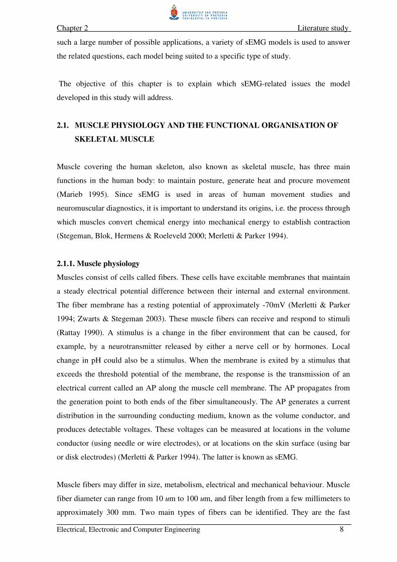
where Pi is the ith line of the power spectrum and M is the highest harmonic considered
(Farina, Mesin & Martina 2004). These two variables provide basic information about the
spectrum of the sEMG signal.
The MDF refers to the frequency value that splits the spectrum into two parts containing
equal power (Farina & Merletti 2000). The MDF and MNF will coincide if the spectrum is
symmetric with respect to its centre line and will be different if the spectrum is skew.
Spectral measurements are strongly influenced by electrode location, thickness of
subcutaneous layers, fiber misalignment, the depth of the source within the muscle, fiber
length, the spatial filter used, electrode size and shape and IED. The following
observations can be made:
• IED: a change in IED will change the spatial transfer function of the detection
system and affect the signal properties. For larger IED more high-frequency non-
propagating components will be included in the computation of the mean
frequency.
• Thickness of subcutaneous layers: since the subcutaneous layers separating the
electrodes from the muscle fibers act as a low-pass filter, MNF will decrease with
increasing thickness. This is also true for the dept of the MU within the muscle.
The MNF for a deeper MU will be subject to a stronger low-pass filter effect
(Farina, Cescon & Merletti 2002; Merletti & Parker 2004).
• Location of electrodes: frequency content is highest near the innervation and
tendon zones, and decreases with distance from these zones. This is again because
of the influence of high-frequency non-propagating components (Merletti, Lo
Conte, Avignone & Guglielminotti 1999a; Roy, De Luca & Schneider 1986).
• Fiber-electrode misalignment: the effect of the inclination of the muscle fibers with
respect to the detection system is difficult to predict. This effect is also dependent
on electrode size and shape, as well as which detection system is used.
• Spatial filter: the spatial filter used determines the attenuation of the end-of-fiber
component. At the same time it also acts as a high-pass filter for the travelling

Chapter 2 Literature study
Electrical, Electronic and Computer Engineering 20
components. When high selective spatial filters are used, the frequency content is
increased (Merletti & Parker 2004).
Observation of spectral content can be used in sports training. A subject can learn how to
control optimal endurance muscle activity through real-time feedback of the frequency
shift during sustained contraction (Devasahayam 2000). However, most research on the
spectral analysis of the sEMG signal is towards the study of muscle fatigue. Muscle fatigue
in itself is not a variable associated with the sEMG signal and its assessment requires the
definition of indexes based on physical variables that can be measured, such as firing rates,
conduction velocity, amplitude or spectral estimates.
2.3.3. Conduction velocity
The CV of a fiber is an indication of the muscle’s functional state. CV is between
3 and 6 m/s, with an average of almost 4 m/s. To measure CV the variables needed are the
IED and the delay between two detected signals. The two signals need to be identical and
time-shifted. That means there has to be such a degree of similarity between the two
signals that an applied time-shift will minimise the mean square error of the one signal
with the other (Farina & Merletti 2000). For sEMG detection of CV, either the cross-
correlation function or the linear system impulse response has to be used. When these
approaches are used, there is a confounding factor to keep in mind. In the signals obtained,
coherent nondelayed EMG components are present. This is because of the termination of
fibers at the tendon-endings. This effect will give rise to a positive bias in the conduction
velocity estimate, and can be reduced by using the DD electrode configuration (Merletti,
Roy, Kupa, Roatta & Granata 1999b; Merletti & Parker 2004; Merletti & Parker 1994).
An important fact to remember when calculating the CV is that the electrodes have to be
aligned with the muscle fibers; misalignment will lead to electrical noise caused by shape
changes to the IAP as well as influences from the non-travelling components (Merletti,
Rainoldi & Farina 2001). This is more apparent in anisotropic systems where the
anisotropy has a significant effect on the shape of the detected IAPs.

Chapter 2 Literature study
Electrical, Electronic and Computer Engineering 21
2.4. APPLICATIONS OF SEMG
In the past decade needle EMG has been seen as the more reliable diagnostic tool.
However, sEMG has been studied extensively, and now shows considerable potential as a
diagnostic tool in human movement studies, neuromuscular disease, clinical
neurophysiology and electrodiagnostic medicine (Stegeman, Blok, Hermens & Roeleveld
2000). SEMG is a non-invasive, inexpensive application giving global information about
muscle physiology and can be used separately or complementary to needle EMG (Zwarts,
Drost & Stegeman 2000; Perry, Schmidt & Antonelli 1981). SEMG is convincingly used
in the kinesiological disciplines, which include rehabilitation science, ergonomics, exercise
and sports physiology (Stegeman, Blok, Hermens & Roeleveld 2000). In addition sEMG
provides an application with which to measure MU location, direction of muscle fibers,
endplate position and fiber-tendon transition and is successfully used in the following
applications:
Myoelectric manifestation of muscle fatigue
Investigating the myoelectric manifestation of muscle fatigue is important in sport,
rehabilitation and occupational medicine. It is also useful in the analysis of back muscle
impairment to solve back problems and lower back pain (Merletti & Parker 1994). Muscle
fatigue produces changes in the characteristics of the sEMG signal (Dimitrova & Dimitrov
2003). After a prolonged isometric contraction, changes in muscle fiber membrane
excitability and in MUAP propagation are detected. If the contraction is maintained, the
muscle metabolic conditions are altered, and if conditions are still maintained, this will
lead to failure of excitation-contraction coupling. This is called mechanical failure
(Merletti, Rainoldi & Farina 2001). Muscle fatigue can be measured with sEMG and is
characterised by a decrease in CV and spectral variables and an increase in amplitude
(Stegeman, Blok, Hermens & Roeleveld 2000; De Luca 2002; Merletti, Rainoldi & Farina
2001; Zwarts, Drost & Stegeman 2000; Zwarts & Stegeman 2003; Roeleveld, Blok,
Stegeman & Van Oosterom 1997a). Muscle fatigue is easier to detect when contractions
are electrically elicited. This implies that the detected signal will be deterministic and not
stochastic.
Estimation of fiber type distribution
Determining fiber types within a muscle is usually investigated with histochemical analysis
or biopsies. The high cost and ethical problems related to this technique of fiber typing is
an excellent reason for exploring non-invasive sEMG as a method for fiber typing. As

Chapter 2 Literature study
Electrical, Electronic and Computer Engineering 22
mentioned before, muscles consist of two types of fibers. Type 2 fibers have a higher CV,
which will decrease faster during sustained contraction. CV and the spectral features of
sEMG are good variables to use for fiber typing. They are related to the pH decrease due to
the increment of metabolites produced during fatiguing contractions (Merletti & Parker
2004). Although more research is needed sEMG can be used as a non-invasive tool for
fiber typing (Merletti, Rainoldi & Farina 2001; Merletti & Lo Conte 1997). This
information is important in sport and geriatric medicine (Merletti et al. 2002), as well as
where fiber type modifications due to diseases or natural adaptation are encountered
(Merletti & Parker 2004).
Measurement of changes induced by training, disuse and aging
Amplitude measurement in sEMG is a reliable variable to use when observing changes in
force output before and after a training session. Changes in the size of MUs are also
reflected in amplitude measurements and can reveal loss of muscle fiber or reinnervation.
The onset of atrophy with aging can also be observed (Merletti, Rainoldi & Farina 2001;
Zwarts & Stegeman 2003; Merletti, Farina, Gazzoni & Schieroni 2002).
Biofeedback
The onset of muscle fatigue is characterised by a shift in frequency of the sEMG signal.
This is due to various physiological effects. Allowing for real-time feedback, it should be
possible to control muscle force at optimal endurance by stabilising the frequency of the
contraction. This allows for the possible enhancing of the voluntary control of muscles.
Gait analysis and muscle activation intervals
With sEMG, complicated movement patterns can be observed. The activation of different
muscle groups during gait analysis can be observed. This information is very useful in
movement disorders such as dystonia and tremor (Zwarts, Drost & Stegeman 2000; De
Luca 2002; Stegeman, Blok, Hermens & Roeleveld 2000; Zwarts & Stegeman 2003). The
relevance of sEMG in kinesiology applications also includes the study of motor control
strategies, the investigation of the mechanics of muscle contraction and the identification
of pathophysiological factors (Merletti & Parker 2004).
Myopathies characterised by membrane disturbances
Abnormal muscle fiber CV is indicative of myopathies characterised by membrane
disturbances. These disturbances occur because of functional disturbances in the ionic

Chapter 2 Literature study
Electrical, Electronic and Computer Engineering 23
channels (Stegeman, Blok, Hermens & Roeleveld 2000; Zwarts, Drost & Stegeman 2000;
Zwarts & Stegeman 2003).
Control of myoelectric prosthesis
The motors of artificial limbs (hands, wrists, elbows) may be controlled by sEMG signals
detected from muscles above the level of amputation (Merletti & Parker 1994).
Occupational medicine and ergonomics
SEMG is used in ergonomic studies to evaluate how workplace factors such as tasks,
posture, tool design and layout influence the activity of a set of muscles (Merletti & Parker
1994).
2.5. LIMITATIONS OF SEMG
Despite increasingly complex sEMG array designs, sEMG still presents some limitations.
SEMG is limited to signal detection of superficial muscles with parallel fibers. Some other
limitations are:
• SEMG is not particularly successful when measured for muscles with pennated
fiber architecture or curved fibers or when multiple IZs are measured (Zwarts,
Drost & Stegeman 2000).
• SEMG detection is sensitive to crosstalk. Crosstalk refers to interference from
muscles other than those containing the electrodes.
• SEMG is also sensitive to other artefacts, for example artefacts due to relative
movement between the electrodes and the skin, or artefacts due to changes in
electrode contact impedance (Merletti & Parker 1994).
• The different design consideration for electrodes can lead to amplitude and
spectral variance in the recording of sEMG signals.
• Tissue filtering attenuates the shape differences of the sEMG signals.
Morphological features have a smaller relevance as classification criteria (De la
Barrera & Milner 1994).
Geometrical factors also have some relevance when evaluating the success of sEMG
measurements. When working under dynamic conditions, the muscles in question will shift
with respect to the skin. This will cause an amplitude change, which can be attributed to
geometrical reasons and not to a different level of muscle activation. This change in
amplitude is mostly because IZ shifts with respect to the skin surface. Little movement of

Chapter 2 Literature study
Electrical, Electronic and Computer Engineering 24
the IZ will provide great amplitude differences in electrodes placed near the IZ. A 1 cm
shift can cause an increase in amplitude of up to 200%, and a 90° change in angle can
cause a 50% change in amplitude (Martin & MacIsaac 2006). Differences caused by
geometrical factors have to be evaluated. The standard deviation of the measured ARV
values is an indication of residual error and defines the resolution one can reach in the
evaluation of geometrical factors. Differences in amplitude can only be attributed to
geometrical factors if they are sufficiently larger than the resolution defined by the
standard deviation (Merletti, Farina & Gazzoni 2002).
2.6. SEMG MODELLING
The most significant reason for sEMG modelling is to establish an approach through which
muscle properties can be related to the measurable variables of the sEMG signal (Merletti,
Lo Conte, Avignone & Guglielminotti 1999a; Farina, Mesin & Martina 2004; Stegeman,
Blok, Hermens & Roeleveld 2000; Farina, Merletti, Nazzaro & Caruso 2001; Rau, Schulte
& Disselhorst-Klug 2004). Signal modelling is also important for understanding the bio-
electric signal generation mechanism, for the testing of processing algorithms, for
detection system design and for the teaching of muscle electrophysiology (Merletti, Lo
Conte, Avignone & Guglielminotti 1999a; Farina, Mesin & Martina 2004). Since sEMG
attempts to answer a number of different questions related to muscle properties,
neuromuscular disorders or even to the control of myoelectric prosthesis, sEMG models
are being developed with increasing complexity and accuracy (Farina, Mesin & Martina
2004). A great number of analytical models are found in literature and more recently also a
variety of numerical models. Recent numerical models were developed by Lowery,
Stoykov, Dewald and Kuiken (2004), Schneider, Silny and Rau (1991), Kuiken, Stoykov,
Popovic, Lowery and Taflove (2001) and Lowery et al. (2002).
SEMG models range from models predicting the behaviour of single muscle fibers to
models producing complete EMG waveform simulations. Different designs of the volume
conductor are used, ranging from infinite flat planes to cylindrical designs. The recent
addition of numerical modelling resulted in more complex volume conductor designs
(Kuiken, Stoykov, Popovic, Lowery & Taflove 2001; Mesin, Farina & Martina 2004). The
electrode detection system has also been redesigned a number of times, leading to a
number of different models. The basic building blocks of sEMG modelling comprise the
source function, the volume conductor and the electrode detection system. Further model
characteristics such as fiber type, number of fibers, tendon and endplate distribution,

Chapter 2 Literature study
Electrical, Electronic and Computer Engineering 25
subcutaneous layers, recruitment and MU firing rate, to name only a few, can further
complicate and enhance sEMG models (Stegeman, Blok, Hermens & Roeleveld 2000).
Generally, sEMG models have been developed for testing sEMG under static isometric
conditions. However, some clinical evaluations, for example gait analysis, can be
understood better if dynamic conditions are incorporated. Recent models have begun to
focus on modelling muscle contractions at different joint angles. This is already a step
closer to dynamic sEMG modelling. When including muscle shortening in an sEMG
model, consideration should be given to geometrical artefacts, for example geometrical
modification of muscle due to fiber shortening and the effect of muscle sliding under the
skin (Farina, Merletti, Nazzaro & Caruso 2001; Schulte, Farina, Merletti, Rau &
Disselhorst-Klug 2004).
This section will explain the different building blocks and characteristics of the sEMG
model. Figure 2.4 is a representation of the possible elements of an sEMG model
(Stegeman, Blok, Hermens & Roeleveld 2000). The model developed in this study
includes some but not all of these building blocks. The black line represents the blocks
included in this study.
Figure 2.4. Schematic representation of the possible elements of an sEMG model
MU source function
Muscle source
function
Volume conductor
Generated
action potentials
Electrode
detection system
Surface action
potentialsFiring and recruitment
Surface EMG
SF source functionSF source function
MU source function
Muscle source
function
Volume conductor
Generated
action potentials
Electrode
detection system
Surface action
potentialsFiring and recruitment
Surface EMG
SF source functionSF source function

Chapter 2 Literature study
Electrical, Electronic and Computer Engineering 26
Each of the elements in figure 2.4 has a number of different design considerations that
relate directly to the type of questions the model under consideration will attempt to
answer.
2.6.1. Source function
The bio-electric source of all neuromuscular activity is found in the outer membrane of a
single muscle fiber. In order to find a definition for the source contained in a single fiber
two assumptions are made. The first assumption implies that the measured potential field is
the linear summation of the potential fields of the contributing muscle fibers. The second
assumption implies that from an sEMG point of view each muscle fiber can be considered
as a line source, thus neglecting its diameter. These two assumptions imply that describing
the IAP wave shape suffices as a source definition (Stegeman, Blok, Hermens & Roeleveld
2000). Equation 2.5, along with its derivative, is a mathematical description often used for
describing the IAP wave shape.
BeAzzVm z −= −λ3)( (2.5)
Vm is the membrane voltage and z the distance along the fiber. Parameters A, B and λ are
responsible for the shape of the IAP. Common values are A = 96 mV for the amplitude of
the action potential and B = -90 mV for the resting membrane potential. λ is a scale factor
expressed in mm-1
, z is the length along the muscle fiber. The membrane current
distribution shown in Equation 2.5 has a triphasic shape and can be simplified to a tripole
source description, which becomes valid for sufficiently large observation distances. To
approximate the tripole, each region of the current source is collapsed into a single
equivalent point source, the sum of which is zero. It is important to know that the tripole
length and intensities are not independent variables and must guarantee physiological
values for the transmembrane action potential amplitude. Thus, if it is assumed that each
active muscle fiber is rectilinear with uniform properties along its length, two tripoles
travelling in the opposite direction can be used as a legitimite source function for
generating measurable action potentials (Merletti, Lo Conte, Avignone & Guglielminotti
1999a; Stegeman, Blok, Hermens & Roeleveld 2000; Farina & Merletti 2001; Rosenfalck
1969). The triangular IAP estimate and the connected tripoles are shown in figure 2.5.

Chapter 2 Literature study
Electrical, Electronic and Computer Engineering 27
Figure 2.5. The triangular estimate of the IAP and the corresponding tripole
Another important consideration in describing the source function is the generation and
extinction of the AP at the NMJ or motor endplate and at the tendon endings. It has to be
taken into account that with extinction the tripole becomes a dipole and finally a
monopole. These effects greatly influence the sEMG signal.
There are sEMG models that only focus on SFAP generation. Muscle fatigue has often
been investigated on this level, resulting in a finding that prolonged repetitive stimulation
of muscle fibers leads to a decrease in CV (Rau, Schulte & Disselhorst-Klug 2004).
However, it is necessary also to have a description of the collective activity of muscle
fibers in an MU. An MU can be modelled by superimposing N single fibers. SEMG
models at this level are different from one another with regard to the variations of fiber
properties they incorporate. Some of the possible variations in properties of single fibers
included in an MU are the following (Merletti, Lo Conte, Avignone & Guglielminotti
1999a; Stegeman, Blok, Hermens & Roeleveld 2000):
• Distribution of motor endplates and of tendon endings. Used in models
investigating neuromuscular disease, optimal electrode placement, size of MUs
and crosstalk.
• Different CVs. Used in models investigating neuromuscular disease, size of MUs,
the calculation of CV from the sEMG interference pattern and muscle fatigue.
• Different fiber types. Used in models investigating questions on the influence of
muscle composition.
NMJ
Right triangular IAP estimateLeft triangular IAP estimate
NMJ
Right tripoleLeft tripole
NMJNMJ
Single muscle fiber of length z
Right triangular IAP estimateLeft triangular IAP estimate
NMJ
Single muscle fiber of length z
Right tripoleLeft tripole
NMJ
Right triangular IAP estimateLeft triangular IAP estimate
NMJ
Right tripoleLeft tripole
NMJNMJ
Single muscle fiber of length z
Right triangular IAP estimateLeft triangular IAP estimate
NMJ
Single muscle fiber of length z
Right tripoleLeft tripole

Chapter 2 Literature study
Electrical, Electronic and Computer Engineering 28
• Relative position of muscle fiber within an MU. Used in models investigating the
position in the muscle from where sEMG signals originate.
• Number of fibers in an MU. Used in models investigating neuromuscular disease,
the number of active MUs for a specific task, muscle forces, positions of tendon
endings and motor endplates.
It can be seen that studies performed at the MU level provide valuable information on
neuromuscular disorders and also on muscle physiology. SEMG is commonly used in
applications in biomechanics, ergonomics and rehabilitation (Rau, Schulte & Disselhorst-
Klug 2004). It is valuable to understand how the sEMG interference pattern is generated.
The modelled surface signal is the superposition of the contributions from M MUs (Rau,
Disselhorst-Klug & Silny 1997). As with the transition from SFs to MUs, there are also a
number of variations that can be included in a model of sEMG generation. These include:
• Number of MUs. Used in models investigating how many MUs are active in a
specific task, influence of muscle composition, muscle fatigue and which central
drive changes can be estimated from the sEMG.
• MU radius. Useful in investigating neuromuscular disorders.
• MU location. Used in models investigating muscle force, sEMG origination,
neuromuscular disorders and the influence of muscle composition.
• Distribution of motor endplates and of tendon endings of the MU. Used in models
investigating how many MUs are active for a specific task.
• CV. Used in models investigating muscle fatigue, calculating CV from an
interference pattern and the influence of muscle composition.
• Force prediction per MU. Used in models investigating muscle force prediction.
When considering the sEMG interference pattern an important aspect to include in the
modelling thereof is the recruitment and firing behaviour of the different MUs. The
recruitment of different MUs during a muscle contraction is directly related to the task at
hand. Movement, speed and direction are task requirements that influence the recruitment
pattern. The size and composition of the muscle will also have an influence on the
recruitment pattern. The firing rate of different MUs is usually chosen between
10 and 50 Hz (Viljoen 2005) and described in terms of the interpulse intervals. MU firing
rate in most cases are activated with a Gaussian distribution (Stegeman, Blok, Hermens &
Roeleveld 2000).

Chapter 2 Literature study
Electrical, Electronic and Computer Engineering 29
2.6.2. Volume conductor
Human tissue acts as a volume conductor, conducting APs from the bioelectric source to
the skin surface. The shape of these APs is greatly influenced by the choice of volume
conductor parameters. The most straightforward description of a volume conductor is to
assume that it is infinite, isotropic, homogeneous and purely resistive. However, in order to
investigate MUAPs accurately at the skin surface it is necessary to include a more complex
volume conductor (Roeleveld, Blok, Stegeman & Van Oosterom 1997a; Stegeman, Blok,
Hermens & Roeleveld 2000).
Anisotropic muscle tissue
Muscle tissue is anisotropic with higher conductivity in the axial direction (the direction of
source propagation) than in the radial direction (the direction perpendicular to the fibers)
(Roeleveld, Blok, Stegeman & Van Oosterom 1997a; Stegeman, Blok, Hermens &
Roeleveld 2000). Although different values for the axial and radial conductivities have
been reported in the literature (Gabriel & Gabriel 2007; Kuiken, Stoykov, Popovic,
Lowery & Taflove 2001), the values are widely accepted as σr = 0.1 Ωm-1
and
σz = 0.5 Ωm-1
(Lowery, Stoykov, Dewald & Kuiken 2004; Roeleveld, Blok, Stegeman &
Van Oosterom 1997a; Lowery, Stoykov, Taflove & Kuiken 2002). In more recent studies a
conductivity tensor has been introduced to determine the local electrical properties of the
volume conductor. The inclusion of a conductivity tensor requires a numerical approach.
Since the conductivity of the muscle tissue depends on the direction of the muscle fiber,
the conductivity tensor of the tissue should depend point-by-point on the fiber orientation
(Farina, Mesin & Martina 2004; Mesin, Farina & Martina 2004).
Finite volume conductor
In sEMG models the muscle fibers are modelled as finite length fibers. This is necessary to
explain the characteristic end-of-fiber effects in the sEMG waveform. The influence of the
finite fiber length is accentuated by the finite dimension of the volume conductor [47]. As
an AP propagates along a path of excitable tissue, the well-known triphasic waveform is
recorded. When the AP encounters the termination of excitable tissue at the tendon
endings, a phenomenon known as the far-field will contribute to the action potential
waveform (Stegeman et al. 1997; Roeleveld, Blok, Stegeman & Van Oosterom 1997a).

Chapter 2 Literature study
Electrical, Electronic and Computer Engineering 30
Inhomogeneity of the surface layers
Since sEMG is recorded on the skin, both a subcutaneous fat layer and the resistive skin
layer can be included in a volume conduction model. Subcutaneous fat layers have low
conductivity and if included in the volume conductor will enhance the amplitude of the
surface action potentials. However, if a better conducting skin layer is also included in the
model, the potential profile is largely averaged out (Roeleveld, Blok, Stegeman & Van
Oosterom 1997a).
Except for the different subcutaneous layers, inhomogeneities are also found within the
excitable tissue. Examples are narrowing and expansion of muscle fiber diameter and a
change in muscle fiber direction. These inhomogeneities are generally found in pinnated
muscles, and have recently been investigated by sEMG models (Mesin, Farina & Martina
2004).
Including capacitive effects
It is generally accepted that volume conductors are quasi-stationary, implying that the
potential field at any moment is determined by the sources at that particular instant only.
This requires that inductive and capacitive effects be ignored, and that the volume
conductor be purely resistive (Lowery, Stoykov, Taflove & Kuiken 2002; Stegeman, Blok,
Hermens & Roeleveld 2000). However, the question of the frequency dependence of EMG
signals caused by the presence of capacitive effects in layered muscle tissue has often
reappeared. In a recent study (Lowery, Stoykov, Dewald & Kuiken 2004), capacitive
effects have been included and this was found to have a noticeable effect on the AP
waveform.
Finite element modelling
SEMG models have predominantly been based on an analytical solution for muscle fibers
located in either finite or infinite volume conductors. Including some of the above
mentioned corrections, for example capacitive effects, in an analytical model complicates
the analytical calculations and the mathematical description becomes extremely difficult to
handle. In order to simulate more complex geometries or include inhomogeneous effects,
numerical methods such as the FE method has been implemented.
Sufficient FE analysis software is available. For sEMG modelling, software with an
efficient geometry modelling ability should be chosen. FE models yield only an

Chapter 2 Literature study
Electrical, Electronic and Computer Engineering 31
approximation to the exact solution of the underlying boundary value problem. When FE
modelling is used the geometry of the volume conductor is discretised into mesh elements.
The potential generated by the electric source is then calculated at each node of the mesh.
Accuracy depends on the size and order of the FE mesh. Fine discretisation of regions with
high intensity of the electric field is necessary. A limitation of numerical modelling is the
computational time; a finer mesh implies greater computational time (Kuiken, Stoykov,
Popovic, Lowery & Taflove 2001; Lowery, Stoykov, Taflove & Kuiken 2002; Zhang, Mak
& Roberts 1998). Figure 2.6 is a representation of a spherical geometry discretised into an
FE mesh.
Figure 2.6. A three-dimensional illustration of a spherical geometry discretised into an FE
mesh
2.6.3. Electrode detection system
The electrode geometry and recording configuration have a significant effect on the
detected surface potential. Except for the monopolar recording configuration, all other
configurations perform spatial filtering on the sEMG signal by a linear combination of the
signals detected by the different electrodes (Merletti & Parker 2004). A computationally
effective way of simulating different electrode configurations is to incorporate the
specified spatial filter with the transfer function of the volume conductor. The fourier

Chapter 2 Literature study
Electrical, Electronic and Computer Engineering 32
transform of the detected potential can then be found by multiplying the fourier transform
of the source by the transfer function of the volume conductor and by the transfer function
of the electrode detection system.
The transfer function of the electrode detection system is linked to the filter mask, which
represents the weighing factors of each electrode. Figure 2.3 E shows a representation of a
Laplace filter. Equation 2.6 shows the filter mask for this electrode configuration
−=
010
141
010
NDDM (2.6)
with MNDD the normal double differential (NDD) Laplace filter mask. The weighted
average of the signals detected by the point electrodes can be viewed as the application to
the potential in spatial domain of a finite impulse response. The spatial transfer function
depends on the number of electrodes, the IED and the weights given to the electrodes.
Equation 2.7 defines the transfer function
∑ ∑−
−=
−
−=
−−=1 1
),(n
mi
h
wr
rdjkidjk
irzxSFzxxx eeakkH (2.7)
where (w+h) is the number of rows in the matrix, (m+n) is the number of columns, air the
weights given to the electrodes, dx the IED in the x direction and dz the IED in the z
direction and kx and kz are the spatial angular frequencies (Merletti & Parker 2004).
Commonly used detection systems in sEMG modelling are the longitudinal (L) SD, LDD,
NDD and inverse binomial of order inverse two (IB2 ) detection systems (Farina, Cescon &
Merletti 2002).
2.6.4. Dynamic modelling
SEMG modelling has mostly been used when investigating isometric contractions during
static conditions. However, there are some clinical applications in which the investigation
of muscle contraction during dynamic conditions could be valuable. These applications
include clinical gait analysis, isokinetic assessment, cyclic movement and estimating the
torque produced about a joint (Clancy, Bouchard & Rancourt 2001; Farina, Merletti,

Chapter 2 Literature study
Electrical, Electronic and Computer Engineering 33
Nazzaro & Caruso 2001; Farina et al. 2004a). The definition of dynamic muscle
contraction is a contraction involving changes in muscles force and/or joint angle as the
contraction progresses (Maslaac, Parker, Scott, Englehart & Duffley 2001). Thus, models
of dynamic sEMG involve the modelling of isometric contractions at different joint angles
(Farina, Merletti, Nazzaro & Caruso 2001; Schulte, Farina, Merletti, Rau & Disselhorst-
Klug 2004; Maslaac, Parker, Scott, Englehart & Duffley 2001). SEMG at different joint
angles is greatly affected by geometrical artefacts related to the fiber shortening, sliding of
the muscle under the skin during movement, changes of the relative location of the muscle
fiber with respect to the detection system and variations in muscle and subcutaneous layer
thickness (Schulte, Farina, Merletti, Rau & Disselhorst-Klug 2004).
Dynamic sEMG modelling is needed to explain which of the above-mentioned artefacts
influences the variables selected as indicators of muscle activation level or muscle fatigue.

Electrical, Electronic and Computer Engineering 34
3. METHODS
A numerical model for the generation of SFAPs in a muscle undergoing various degrees of
fiber shortening is developed. The muscle is assumed to be fusiform with muscle fibers
following a curvilinear path described by a Gaussian function. Different degrees of fiber
shortening are simulated by changing the parameters of the fiber path and maintaining the
volume of the muscle constant. The conductivity tensor is adapted to the muscle fiber
orientation. In each point of the volume conductor, the conductivity of the muscle tissue in
the direction of the fiber is larger than that in the transversal direction. Thus, the
conductivity tensor changes point-by-point with fiber shortening, adapting to the fiber
paths. An analytical derivation of the conductivity tensor is provided. The volume
conductor is then studied with an FE approach using the analytically derived conductivity
tensor. The model is extended to simulate MUAPs and results are obtained to show the
effects of geometrical changes on the AP shape and on AP amplitude and spectral content.
The muscle chosen for this sEMG model is the biceps brachii muscle. The muscle fibers of
the biceps brachii run parallel to one another and the muscle is situated near the skin
surface. Muscle or fiber shortening is achieved by varying the joint angle of the elbow.
Five stages of fiber shortening are simulated.
A complex geometry is chosen and to include the conductivity tensor as well as simulate
shortening, a numerical solution is implemented. The model is developed using FEs. The
software used is FEMlab 3.0.
Figure 3.1 presents an overview of the sEMG model developed for this study.

Chapter 3 Methods
Electrical, Electronic and Computer Engineering 35
Figure 3.1. A block diagram illustrating the development of the sEMG model
Defining the geometry of the volume conductor
Optimize the geometry for minimal computational time
Define the parameters for fiber shortening
Calculate the conductivity tensor from
the fiber path( )
( ) ( ) ( )( ) ( ) ( )( ) ( ) ( )
++−−−−
−−++−
−−−++
++=
tltltl
tltltl
tltltl
yxzwyzwxzw
yzwzxwzyxyz
xzwxyzzywzx
yxzwσσσσσσ
σσσσσσ
σσσσσσ
σ
222422
2224222
2222422
2224
1
Interpolation of APs and applying different electrode
configurations
Extenting model to simulate MUAPs
Describe the source
Numerical implementation
Define the fiber path
Defining the geometry of the volume conductor
Defining the geometry of the volume conductor
Optimise the geometry for minimal computational time
Define the parameters for fiber shorteningDefine the parameters for fiber shortening
Calculate the conductivity tensor from
the fiber path( )
( ) ( ) ( )( ) ( ) ( )( ) ( ) ( )
++−−−−
−−++−
−−−++
++=
tltltl
tltltl
tltltl
yxzwyzwxzw
yzwzxwzyxyz
xzwxyzzywzx
yxzwσσσσσσ
σσσσσσ
σσσσσσ
σ
222422
2224222
2222422
2224
1
Calculate the conductivity tensor from
the fiber path( )
( ) ( ) ( )( ) ( ) ( )( ) ( ) ( )
++−−−−
−−++−
−−−++
++=
tltltl
tltltl
tltltl
yxzwyzwxzw
yzwzxwzyxyz
xzwxyzzywzx
yxzwσσσσσσ
σσσσσσ
σσσσσσ
σ
222422
2224222
2222422
2224
1
Interpolation of APs and applying different electrode
configurations
Extenting model to simulate MUAPsExtending model to simulate MUAPs
Describe the source
Numerical implementation
Numerical implementation
Define the fiber path
Defining the geometry of the volume conductor
Defining the geometry of the volume conductor
Optimize the geometry for minimal computational time
Define the parameters for fiber shorteningDefine the parameters for fiber shortening
Calculate the conductivity tensor from
the fiber path( )
( ) ( ) ( )( ) ( ) ( )( ) ( ) ( )
++−−−−
−−++−
−−−++
++=
tltltl
tltltl
tltltl
yxzwyzwxzw
yzwzxwzyxyz
xzwxyzzywzx
yxzwσσσσσσ
σσσσσσ
σσσσσσ
σ
222422
2224222
2222422
2224
1
Calculate the conductivity tensor from
the fiber path( )
( ) ( ) ( )( ) ( ) ( )( ) ( ) ( )
++−−−−
−−++−
−−−++
++=
tltltl
tltltl
tltltl
yxzwyzwxzw
yzwzxwzyxyz
xzwxyzzywzx
yxzwσσσσσσ
σσσσσσ
σσσσσσ
σ
222422
2224222
2222422
2224
1
( )
( ) ( ) ( )( ) ( ) ( )( ) ( ) ( )
++−−−−
−−++−
−−−++
++=
tltltl
tltltl
tltltl
yxzwyzwxzw
yzwzxwzyxyz
xzwxyzzywzx
yxzwσσσσσσ
σσσσσσ
σσσσσσ
σ
222422
2224222
2222422
2224
1
Interpolation of APs and applying different electrode
configurations
Extenting model to simulate MUAPsExtenting model to simulate MUAPs
Describe the source
Numerical implementation
Numerical implementation
Define the fiber path
Defining the geometry of the volume conductor
Defining the geometry of the volume conductor
Optimise the geometry for minimal computational time
Define the parameters for fiber shorteningDefine the parameters for fiber shortening
Calculate the conductivity tensor from
the fiber path( )
( ) ( ) ( )( ) ( ) ( )( ) ( ) ( )
++−−−−
−−++−
−−−++
++=
tltltl
tltltl
tltltl
yxzwyzwxzw
yzwzxwzyxyz
xzwxyzzywzx
yxzwσσσσσσ
σσσσσσ
σσσσσσ
σ
222422
2224222
2222422
2224
1
( )
( ) ( ) ( )( ) ( ) ( )( ) ( ) ( )
++−−−−
−−++−
−−−++
++=
tltltl
tltltl
tltltl
yxzwyzwxzw
yzwzxwzyxyz
xzwxyzzywzx
yxzwσσσσσσ
σσσσσσ
σσσσσσ
σ
222422
2224222
2222422
2224
1
Interpolation of APs and applying different electrode
configurations
Extenting model to simulate MUAPsExtending model to simulate MUAPs
Describe the source
Numerical implementation
Numerical implementation
Define the fiber path

Chapter 3 Methods
Electrical, Electronic and Computer Engineering 36
3.1. MODEL GEOMETRY
The biceps brachii muscle is modelled as a fusiform volume conductor. For this study the
volume conductor comprises muscle and tendon only. Subcutaneous layers i.e. skin and fat
layers, are ignored.
When muscle contraction is initiated an AP causes depolarisation of a segment of muscle
fiber. This depolarised zone is the source of a potential distribution detectable on the skin
surface (Merletti, Lo Conte, Avignone & Guglielminotti 1999a). For the model developed
in this study a tripole approximation of the source propagates along the fiber path to create
the depolarisation of the muscle fiber and the simulated surface potential. To define the
fusiform geometry of the muscle, the fiber paths are described by means of the following
cylindrical curves:
,)sin()(
)cos()(
)(
=
z
zr
zr
z θ
θ
γ (3.1)
where θ identifies the radial location of the muscle fiber, and r(z) is the distance of the
fiber from the z-axis (central axis of the muscle).
Since the model used in this study ignores the outer skin or fat layers, the external-most
fibers also create the outline of the fusiform volume conductor. The external-most fibers or
basic muscle form is then characterised by a radius )()( zfzr = .
Equation 3.2 defines )(zf :
2
2
2Re)( w
z
zf
−
= , (3.2)
where R is the maximum radius of the muscle tissue. )(zf is illustrated as the outline of
the muscle shown in figure 3.2.
The function )(zf is limited to the interval [ ]ddz ,−∈ , such that the minimum muscle
radius, shown in Equation 3.3,
2
2
20 Re w
d
R
−
= , (3.3)

Chapter 3 Methods
Electrical, Electronic and Computer Engineering 37
corresponds to the chosen tendon thickness. d is the half-length of the muscle as illustrated
in figure 3.2. The parameters R and w determine the geometry of the muscle. For
example, increasing w will increase the muscle length, implying a more relaxed muscle.
Decreasing w will lead to a larger muscle radius and a shorter muscle length, implying a
more contracted state. This description allows for a change in muscle geometry by varying
only two parameters. Figure 3.2 is a two-dimensional representation of the muscle
geometry as defined for the simulation model.
Figure 3.2. A two-dimensional view of the volume conductor’s geometry. The muscle
geometry has a tendon radius R0 of 10 mm and a maximum radius R of 18.5 mm. Rt is the
distance of the fiber from the z axis at the tendon level. Both superficial and deep fibers are
shown. As per definition, the superficial fibers are more curved than the deep fibers.
Figure 3.2 also shows the geometrical difference in superficial and deep fibers. Superficial
fibers are more curved than deep fibers. The conductivity tensor depends point-by-point on
the curvature of the fiber. This implies that not only is there a difference in the electrode-
source distance but also in the conductive properties of superficial and deep fibers. These
Deep fiber
Superficial fibers
R0,
tendon
radius
10 mm
Tendon
z
r(z)
d d
z=0
Geometry of the biceps brachii muscle as defined for the model
R, maximum radius of
volume conductor
Tendon
z=-d z=d
f(z)
muscle fiber
Deep fiber
Superficial fibers
R0,
tendon
radius
10 mm10 mm
Tendon
z
r(z)
d d
z=0
Geometry of the biceps brachii muscle as defined for the model
R, maximum radius of
volume conductor
Tendon
z=-d z=d
Rt
f(z) , external-mostmuscle fiber
Deep fiber
Superficial fibers
R0,
tendon
radius
10 mm10 mm
Tendon
z
r(z)
d d
z=0
Geometry of the biceps brachii muscle as defined for the model
R, maximum radius of
volume conductor
Tendon
z=-d z=d
f(z)
muscle fiber
Deep fiber
Superficial fibers
R0,
tendon
radius
10 mm10 mm
Tendon
z
r(z)
d d
z=0
Geometry of the biceps brachii muscle as defined for the model
R, maximum radius of
volume conductor
Tendon
z=-d z=d
Rt
f(z) , external-mostmuscle fiber

Chapter 3 Methods
Electrical, Electronic and Computer Engineering 38
details are illustrated in chapters 4 and 5, where the results of the simulations are
discussed.
As the joint angle of the elbow is decreased, the biceps brachii muscle shortens. To
simulate muscle shortening only two parameters, the width w and the radius R have to be
changed. To represent the biceps brachii muscle accurately at five different stages of
shortening, the values for w and R have to be calculated. In order to calculate these values
two constraints are imposed:
1) the volume V of the muscle has to remain constant,
2) the minimum radius, R0 (the radius of the tendon), has to remain constant for
each shortening condition.
Equation 3.4 imposes the first constraint:
∫ ∫Ω−
===d
dw
dErfwRdzzrdVV )()( 2
3
22 ππ = constant, (3.4)
with
λπ
λdezErf
z
∫−=
0
22)( (3.5)
The second constraint imposes f(d)=R0, leading to the relation shown in Equation 3.6:
=
0
ln2R
Rwd . (3.6)
Substituting Equation 3.6 into Equation 3.5 one obtains Equation 3.7:
=
0
0
2
2
3
2 ln2*
ln2R
RErf
R
R
dRV π . (3.7)

Chapter 3 Methods
Electrical, Electronic and Computer Engineering 39
Given the volume of the muscle V, the length of the muscle d and the radius R0 of the
tendon, the value of R can be calculated from Equation 3.7. This is a numerical calculation.
When R is determined the parameter w is obtained by Equation 3.6. The parameter w is the
same for all fibers. The maximum distance RRd ≤ of each fiber from the z axis is
computed by assuming the ratio RRd / constant in each shortening condition. In this way,
fiber density is the same in each point of the muscle section. Table 3.1 gives the calculated
simulation parameters for the five stages of shortening.
Table 3.1. Model parameters
Model
Parameter
Stage 1
Stage 2 Stage 3 Stage 4 Stage 5
R0 10 mm 10 mm 10 mm 10 mm 10 mm
R 15 mm 16.5 mm 18.5 mm 21 mm 23 mm
L 150 mm 130 mm 110 mm 90 mm 80 mm
w 83.29 64.95 49.58 36.94 30.99
V 83.2 cm3 83 cm
3 83.4 cm
3 83 cm
3 85.1 cm
3
CV 4 m/s 4 m/s 4 m/s 4 m/s 4 m/s
Stage 1 assumes a relaxed muscle condition. This stage is the reference. The percentage
shortening for the other stages are computed with respect to the reference stage. For the
reference stage a maximum radius R of 15 mm was chosen based on anatomical data from
the literature (Viljoen 2005). The biceps brachii muscle has a limited range of fiber lengths
over which the muscle can operate effectively. The optimal muscle fiber length is chosen
as d =150 mm (Garner & Pandy 2003). Since muscle tissue cannot generate active muscle
force beyond 0.5 times the optimal length (Garner & Pandy 2003), the four remaining
stages of shortening were chosen within this constraint. The volume for the relaxed stage
was calculated and kept constant for the following stages. The volume conductor for five
stages of shortening is shown in figure 3.3.

Chapter 3 Methods
Electrical, Electronic and Computer Engineering 40
13.3 % shortening
26.7 % shortening
L0 = 150 mm
L1 = 130 mm
L2 = 110 mm
L3 = 90 mm
L4 = 80 mm
40 % shortening
46.6 % shortening
Tendon TendonMuscle
Reference condition
Figure 3.3. A two-dimensional view of the volume conductor for five stages of
shortening. As the muscle geometry shortens, the volume increases. The tendon
regions remain of the same length and diameter for all conditions.
3.2. CONDUCTIVITY TENSOR
In less complex models the conductivity of muscle tissue was described using constant
values for the longitudinal and transversal conductivities (Lowery, Stoykov, Taflove &
Kuiken 2002). The model presented in this work attempts to simulate changes in the
surface potential representative of a change in the electrical properties of the muscle tissue.
To integrate this change with the geometrical changes due to muscle shortening, the local
electrical properties of the volume conductor are fully determined by its conductivity
tensor. The conductivity tensor has to be related to the curve describing the fiber path. A
general conductivity tensor is described in Equation 3.8. The conductivity tensor of
Equation 3.8 procreates with the vector describing the fiber path in order to produce a new

Chapter 3 Methods
Electrical, Electronic and Computer Engineering 41
vector, which is linearly related to the old one, but now points in the direction of source
propagation ( 2004).
In order to have an advanced numerical description of the volume conductor, an accurate
description of the conductivity tensor for the muscle tissue is required. Since the
conductivity of the muscle tissue depends on the direction of the muscle fibers, the
conductivity tensor of this tissue should depend point-by-point on the fiber orientation
(Farina, Mesin & Martina 2004).
A general conductivity tensor for muscle tissue is expressed in Equation 3.8:
tbtbttntntlll ννσννσννσσ ˆˆˆˆˆˆ ++= , (3.8)
where the subscript l stands for longitudinal and t for transversal coordinates with respect
to fiber direction. Thus ,, tnl νν and tbν are the longitudinal, normal and binormal versors
relative to the fiber orientation, respectively. Such versors are functions of the position in
case of curvilinear fibers (Farina, Mesin & Martina 2004; Mesin, Joubert, Hanekom,
Merletti & Farina 2006).
Since the bioelectrical problem of EMG simulation can be considered quasi-statical,
implying that the potential field at any moment is determined by the sources at that same
instant (Merletti & Parker 2004), the Poisson equation holds. Poisson’s equation is shown
in Equation 3.9:
Ω∂=∇
Ω=∇⋅∇−
0ϕσ
ϕσ g)(, (3.9)
where σ is the conductivity tensor, ϕ the electric potential, g the source term (which is a
current density travelling along the fiber and inducing its contraction), Ω and Ω∂ the
volume conductor domain and its boundary, respectively. Poisson's equation links
potentials directly to the sources producing them (Plonsey & Barr 2000).
Different volume conductors can be modelled by choosing a conductivity tensor that is
related to the volume conductor shape (Mesin, Farina & Martina 2004). Since the fiber

Chapter 3 Methods
Electrical, Electronic and Computer Engineering 42
path is given in cylindrical coordinates, translation is necessary. Poisson’s equation, in a
Cartesian system for the general conductivity tensor introduced above, can be obtained by
introducing the Cartesian representation of the curvilinear differential operators (gradient
and divergence). This is represented by Equation 3.10:
( )( ) ( ) ( )
∂
∂
∂
++∂∂∂=•∇⋅∇
z
y
x
tbtbttntntlllzyx vvvvvv ˆˆˆˆˆˆ σσσσ , (3.10)
where x∂ , y∂ and z∂ indicate the partial derivative operators in Cartesian coordinates.
Equation 3.10 can be used in general to determine the conductivity tensor given the
propagation path of the source (Farina, Mesin & Martina 2004). For the propagation path
given in Equation 3.1, the longitudinal versor lν is calculated by taking the first derivative
with respect to z. The binormal versor tbν is calculated by taking the first derivative with
respect to θ , and the normal versor tnν is calculated by taking the cross product of the
longitudinal and binormal versors. For the fusiform muscle introduced, the longitudinal,
normal, and binormal vectors translated into Cartesian coordinates become:
( )( ) ;
11
sin
cos
2
2
−
−
=
=w
zyw
zx
r
r
vl θ
θ
&
&ρ
( )( ) ;sin
cos
22
2
22
22
+
+
+
=
−
=
yxw
z
yx
y
yx
x
r
vtn
&
ρθ
θ
+
+−
=
−
=
00
)cos(
)sin(
22
22
yx
x
yx
y
vtb θ
θρ
(3.11)

Chapter 3 Methods
Electrical, Electronic and Computer Engineering 43
where the point over a symbol indicates the first derivative with respect to z. Using their
normalised versions in the general expression for a conductivity tensor described in
Equation 3.10, calculations yield the following expression (Equation 3.12) of the
conductivity tensor in a Cartesian system for the fusiform muscle defined by the fiber
orientation of Equation 3.1.
( )
( ) ( ) ( )( ) ( ) ( )( ) ( ) ( )
++−−−−
−−++−
−−−++
++=
tltltl
tltltl
tltltl
yxzwyzwxzw
yzwzxwzyxyz
xzwxyzzywzx
yxzwσσσσσσ
σσσσσσ
σσσσσσ
σ222422
2224222
2222422
2224
1
(3.12)
Equation 3.12 is the tensor to be used in an FE model for describing the conductivity
properties of the muscle tissue point-by-point under different degrees of fiber shortening.
Equation 3.10 provides a general way to compute the conductivity tensor, given the
direction of the muscle fibers. In general, given the parametric representation of the curve
defining the muscle fiber, it is possible to compute the corresponding normal, binormal and
longitudinal versors, and from there the determination of the conductivity tensor (Farina,
Mesin & Martina 2004).
The specific muscle shape and the way to simulate shortening are not a constraint of the
proposed model. By deriving the Cartesian representation of the conductivity tensor
starting from the analytical description of the fiber orientation, the concepts proposed in
this study can be applied to generic muscle shapes and fiber orientations.
3.3. SOURCE DESCRIPTION
The modelling of the generation, propagation, and extinction of the IAP has been
extensively addressed in the literature (Dimitrov & Dimitrova 1998; Duchêne & Hogrel
2000; Lowery, Stoykov, Taflove & Kuiken 2002; Griep, Gielen, Boon, Hoogenstraten,
Pool & Wallinga de Jonge 1982). The general assumption is that the integral of the current
density over the muscle fiber length is zero in each instant of time. For volume conductors
that are not space-invariant in the direction of propagation, as the one studied in this work,
the response of the system to an impulsive current depends on the position of the current
(thus, it is not an impulse response in the sense of linear and space-invariant spatial

Chapter 3 Methods
Electrical, Electronic and Computer Engineering 44
filtering). The source function should be sampled and viewed as a multi-pole. In sEMG
modelling it is accepted that the detection electrodes are a sufficient distance from the
source and that the AP voltage Vm(z) described in Equation 2.5 can be approximated as a
tripole (Merletti & Parker 2004). For the field source implemented in this model the tripole
approximation of the transmembrane current density was used (Mcgill & Huynh 1988).
The tripole equations connected to Equation 2.5 are defined in Equations 3.13 and 3.14:
0321 =++ III (3.13)
032 =+ bIaI (3.14)
I1, I2, and I3 represent the values for the three current impulses. a and b are the distances
between impulses. For the source implemented in this work the values for Equations 3.13
and 3.14 are given in table 3.2.
Table 3.2. Current source parameters
Model parameters Values
I1 24.6
I2 -35.5
I3 10.8
a 2.1
b 6.9
Generation (at the NMJ) and extinction (at the tendon) of the IAPs have very important
implications for the resulting simulations. For the tripole approximation the three poles are
coincident at the NMJ at the moment of excitation. The first pole then moves in discrete
steps for distance a, the second moves with the first for distance b until finally the tripole
propagates as a unit along the fiber path. For the extinction at the tendon ending, the
opposite effect takes place. The first pole reaches the ending and stops, leaving the second
and third poles to form a dipole moving towards the tendon. Finally the three poles overlap
and cancel out. Figure 3.4 is a three-dimensional FE representation of the movement of the
tripole towards the tendon ending.

Chapter 3 Methods
Electrical, Electronic and Computer Engineering 45
Figure 3.4. A) The tripole is propagating along the fiber path. B) The first pole is at the
tendon ending, leaving the second and third poles to propagate as a dipole. C) Extinction of
the tripole
The path of propagation of the transmembrane current was defined by the curve γ in
Equation 3.1, which also determined the conductivity tensor. The arch length of γ was
used as the coordinate to locate the tripole source within the muscle and to describe its
propagation (Farina, Mesin & Martina 2004).
3.4. NUMERICAL IMPLEMENTATION
The numerical approach applied was based on FEs and implemented by the software
package FEMLAB (version 3.0a). The boundary conditions for the muscle were
homogeneous Neumann conditions (Silvester & Ferrari 1983). A Neumann boundary (also
referred to as natural boundary) condition specifies the value of the normal flux across the
boundary. By the image theorem, Neumann boundary conditions lead to periodicity
(Silvester & Ferrari 1983). A sub-domain representing the tendon ending was added to the
muscle geometry (Figure 3.1) in order to reduce aliasing. The periodicity given by the
Neumann boundary conditions can be used to reduce computational time. From image
theory, cutting the muscle geometry in two halves, it is possible to study two propagating
A) B)
C)
A) B)
C)

Chapter 3 Methods
Electrical, Electronic and Computer Engineering 46
tripoles by simulating only one (the second is an image of the first). Thus, in order to save
computational time, only half of the original volume conductor can be described (the
halved volume conductor is presented in figure 3.5), imposing the Neumann boundary
conditions at z = 0, which account for the second half of the volume conductor (image of
the first half). This approach is valid only for symmetric muscle fibers, with the end-plate
in the middle of the volume conductor. If the muscle fibers are asymmetric, the entire
volume conductor and the two tripoles should be studied.
The tendon ending was considered isotropic (conductivity 0.3 S/m), while the muscle
tissue was electrically described by the conductivity tensor in Equation 3.12 (in-
homogeneous and anisotropic), with σl and σt 0.5 S/m and 0.1 S/m, respectively.
To calculate the surface potential, the source was moved step-wise along the fiber path
described by Equation 3.1. Given the conduction velocity v of the IAP and the sampling
rate fs in the time domain, v/fs is the step by which the source is moved between two
sampling instants. For each sampling instant, the potential distribution over the entire
muscle surface was computed by meshing the volume conductor using tetrahedral
elements. This is shown in figure 3.5.

Chapter 3 Methods
Electrical, Electronic and Computer Engineering 47
10 mm
Figure 3.5. A three-dimensional view of the volume conductor described by finite
elements. Because of image theory, the muscle geometry has been halved (see text for
details). The volume conductor (muscle and tendon) is meshed into approximately
100 000 tetrahedral elements.
The elements surrounding the source were smaller than the others (maximum diameter of
these elements 0.1 mm), to improve accuracy. The potential was calculated at the nodes
located at the vertices of the tetrahedral elements (Lowery, Stoykov, Taflove & Kuiken
2002). Point electrodes were simulated. To obtain the potential at the muscle surface
corresponding to the exact location of the electrode, the potential values at the four nodes
nearest to the detection point were interpolated. This was done by calculating the distance
of each node from the electrode and summing the potentials at the nodes by a convex linear
combination (i.e., with unitary sum of the weights) with weights proportional to the inverse
of the distances (which is the rate of decrease of the free-space potential in the three-
dimensional space, neglecting the effect of anisotropy within the specific element). Figure
3.6 shows the solution obtained with FEMLAB for the geometry of figure 3.5 when the
source of section 3.3 propagates along the fiber path.

Chapter 3 Methods
Electrical, Electronic and Computer Engineering 48
Figure 3.6. Solution obtained with FEMLAB for the tripole source propagating along the
volume conductor. The darker red patches represent the positive poles of the tripole, and the
blue patch represents the negative pole.
3.5. ANALYTICAL GENERATION OF MUAPS
The model created in this work was used to create libraries of extracellular potentials for
SFs. These libraries consist of potentials calculated at 2 mm steps along the fiber path.
Seven different fiber depths are simulated and, for each fiber depth, potentials are obtained
for five different muscle shortenings. These libraries are then used to expand the model
and include the simulation of MUAPs. An MU is modelled as the summation of N parallel
fibers uniformly distributed inside a cylinder of radius R (Merletti, Lo Conte, Avignone &
Guglielminotti 1999a). For the model expansion it is assumed that all fibers in the MU are
located at the same cross-sectional location and are of equal CV (4 m/s). These
assumptions were also used in previous works (Lowery, Stoykov & Kuiken 2003). The
number of fibers inside a single MU of the biceps brachii muscle is found to vary
significantly. Numbers of between 50 and 700 have been reported in the literature (Viljoen
2005). It was decided to use 300 fibers in each of the MUs. Before the single fibers are
summed into the MUs, the NMJ or end-plate of the indivivual fibers are uniformly
distributed throughout a zone of 12 mm. This uniform distribution is repeated at the tendon

Chapter 3 Methods
Electrical, Electronic and Computer Engineering 49
junction. MUs are now created at seven depths and for five muscle shortenings.
Representative results for the MUAPs are shown in chapter 5.

Electrical, Electronic and Computer Engineering 50
4. RESULTS: EFFECT OF
MUSCLE SHORTENING ON
SFAPS
4.1. OBJECTIVE
Chapter 3 describes the FE model developed in this study. The aim of this study is to
develop a simulation model, which could bring to light the influence of muscle shortening
when a complex analytical conductivity tensor is included.
The results obtained from simulations prepared with this model are presented in chapter 4.
Simulations were prepared to generate SFAPs on the muscle surface at five stages of
shortening. SFAPs were generated for fibers situated at seven different depths. The
parameters related to the five geometries are reported in Table 3.1. The APs were recorded
using monopolar, SD and DD detection systems. The objective is to validate the model at a
single fiber level as well as to highlight the geometrical artifacts brought about by muscle
shortening as well as changes in the electrical properties of the muscle tissue. The muscle
modelled is the biceps brachii muscle.
An analytical expansion of the model is used to generate MUAPs. Since MUs comprise
single fibers with uniformly distributed NMJs, it is important to validate the model at the
single fiber level. Results for simulations prepared for MUAPs are shown in chapter 5.

Chapter 4 Results: Effect of muscle shortening on SFAPs
Electrical, Electronic and Computer Engineering 51
4.2. METHODS
To generate the APs the tripole source was moved along the propagation path using 2 mm
steps. The surface potential at the recording electrode was then calculated by interpolating
the four surface potentials nearest to the detection point. This was done by calculating the
distance of each node from the electrode, and summing the potentials at the nodes by a
convex linear combination with weights proportional to the inverse of the distances. The
recording electrode system was placed over the surface of the muscle between the fiber
end-plate and the tendon ending in all conditions. The longitudinal muscle shift with
respect to the electrodes, which probably occurs in experimental recordings, was not
considered in the simulation results shown in this chapter. The muscle shift, however, is
included in the simulation of the MUAPs that follow in chapter 5. Monopolar, SD, and DD
recording systems are simulated. For single and double differential detection, the IED is
5 mm and the electrode detection system is placed directly over the fiber.
Except for the surface potentials shown for the three recording systems, two other
processing techniques known as the ARV and the MNF are used to interpret results on the
amplitude and spectral content of the potentials. The ARV is an amplitude estimator and
can be calculated with Equation 2.1 shown in chapter 2. The MNF is a variable that
provides information on the spectral content of the signal and can be calculated with
Equation 2.3 shown in chapter 2.
4.3. RESULTS
4.3.1. SFAPs detected over the muscle surface
Figures 4.1 - 4.3 show the SF surface potentials detected by the different electrode
configurations for the five stages of muscle shortening. Figure 4.1 presents the monopolar
detection system. Figure 4.2 presents the SD detection system and figure 4.3 the DD
detection system. Each figure represents the surface potentials measured for fibers at two
depths. The two depths presented are located within the muscle corresponding at the
tendon location to a distance of Rt = 6.25 mm (representing deep fibers) and Rt = 8.75 mm
(representing more superficial fibers). The IED for the SD and DD detection systems is
5 mm. The electrodes are placed directly over the fiber.

Chapter 4 Results: Effect of muscle shortening on SFAPs
Electrical, Electronic and Computer Engineering 52
40% 46.6%
Reference condition
13.3% 26.7% shortening
40% shortening shortening
A)
B)
13.3% 26.7% shortening
Radiu
s 8.7
5 m
mR
adiu
s 6.2
5 m
m
20 ms
0.0
25 A
U
20 ms
1 A
U
Figure 4.1. Monopolar detected surface potentials generated at five stages of shortening.
Potentials are shown for a superficial and a deep fiber. AU stands for arbitrary units.
40% 46.6%
Reference condition
13.3% 26.7% shortening
40% shortening shortening
A)
B)
13.3% 26.7% shortening
Radiu
s 8.7
5 m
mR
adiu
s 6.2
5 m
m
20 ms
0.0
25 A
U
20 ms
1 A
U
Figure 4.2. SD detected surface potentials generated at five stages of shortening. Potentials
are shown for a superficial and a deep fiber. AU stands for arbitrary units.

Chapter 4 Results: Effect of muscle shortening on SFAPs
Electrical, Electronic and Computer Engineering 53
40% 46.6%
Reference condition
13.3% 26.7% shortening
40% shortening shortening
A)
B)
13.3% 26.7% shortening
Radiu
s 8
.75 m
mR
adiu
s 6
.25 m
m
20 ms
0.0
25 A
U
20 ms
1 A
U
Figure 4.3. Double differential surface potentials generated at five stages of shortening.
Potentials are shown for a superficial and a deep fiber. AU stands for arbitrary units.
Discussion
For the surface potentials shown in figures 4.1 to 4.3, a noticeable difference can be seen
between potentials detected for a deep fiber and potentials detected for a superficial fiber.
The influence of muscle shortening is clearly identifiable, and in all probability enhanced
by the inclusion of a conductivity tensor. The amplitude of the propagating part of the
potential significantly reduces while that of the non-propagating part clearly increases. The
difference for potentials detected with different electrode detection systems is also clear.
The DD detection system is more selective than both the SD and monopolar systems. The
DD detection system also reduces the end-of-fiber effects more successfully.
4.3.2. MNF and ARV as estimators for amplitude and spectral content
Figures 4.4 and 4.5 show the ARV and MNF computed at seven different fiber depths and
for the five stages of shortening shown in figure 3.3. Three detection systems are
compared: monopolar, SD and DD. Both the ARV and MNF values are recorded at 0°
from the fiber and normalised with respect to values obtained for the relaxed muscle

Chapter 4 Results: Effect of muscle shortening on SFAPs
Electrical, Electronic and Computer Engineering 54
condition. The fiber is located within the muscle at seven depths, corresponding at the
tendon location to a distance Rt from the z axis (see figure 3.1). Rt is in the range
1.25 mm – 8.75 mm (1.25 mm increments). A small Rt implies a deep fiber. Electrodes are
located in the middle between the end plate and the tendon in all conditions. Again, for
single and double differential detection, the IED distance was 5 mm.
Figure 4.4. ARV computed from simulated muscle fiber APs for seven different depths and
for the five muscle lengths given in table 3.1. Monopolar, single and double differential
detected potentials are shown. Rt = 1.25 mm represents the deepest fiber.
Discussion
The ARV estimator shown in figure 4.4 is normalised with respect to stage 1, the relaxed
muscle. It is clear that the amplitude decreases as the muscles shortens. This effect is more
noticeable for deeper fibers, especially for the DD detection system. The monopolar
detection system seems to be less affected by a change in muscle length, especially for the
deeper fibers. This might be unexpected, but is easily explained if the influence of the non-
propagating part of the signal (see figure 4.1) is kept in mind. For superficial fibers the
influence of the type of detection system used is less. This can be seen from the graph for
80 90 100 110 120 130 140 150
0.2
0.4
0.6
0.8
1
1.2
80 90 100 110 120 130 140 150
0.2
0.4
0.6
0.8
1
1.2
80 90 100 110 120 130 140 150
0.2
0.4
0.6
0.8
1
1.2
80 90 100 110 120 130 140 150
0.2
0.4
0.6
0.8
1
1.2
80 90 100 110 120 130 140 150
0.2
0.4
0.6
0.8
1
1.2
80 90 100 110 120 130 140 150
0.2
0.4
0.6
0.8
1
1.2
Monopolar
Single differential
Double differential
80 90 100 110 120 130 140 150
0.2
0.4
0.6
0.8
1
1.2
Muscle length (mm)
AR
V (
No
rmaliz
ed u
nits)
Muscle length (mm) Muscle length (mm) Muscle length (mm)
Muscle length (mm) Muscle length (mm) Muscle length (mm)
AR
V (
Norm
aliz
ed u
nits)
AR
V (
No
rmaliz
ed u
nits)
Rt = 1.25 mm Rt = 2.5 mm Rt = 3.75 mm
Rt = 5 mm Rt = 6.25 mm Rt = 7.5 mm
Rt = 8.75 mm
80 90 100 110 120 130 140 150
0.2
0.4
0.6
0.8
1
1.2
80 90 100 110 120 130 140 150
0.2
0.4
0.6
0.8
1
1.2
80 90 100 110 120 130 140 150
0.2
0.4
0.6
0.8
1
1.2
80 90 100 110 120 130 140 150
0.2
0.4
0.6
0.8
1
1.2
80 90 100 110 120 130 140 150
0.2
0.4
0.6
0.8
1
1.2
80 90 100 110 120 130 140 150
0.2
0.4
0.6
0.8
1
1.2
Monopolar
Single differential
Double differential
Monopolar
Single differential
Double differential
80 90 100 110 120 130 140 150
0.2
0.4
0.6
0.8
1
1.2
Muscle length (mm)
AR
V (
No
rmaliz
ed u
nits)
Muscle length (mm) Muscle length (mm) Muscle length (mm)
Muscle length (mm) Muscle length (mm) Muscle length (mm)
AR
V (
Norm
aliz
ed u
nits)
AR
V (
No
rmaliz
ed u
nits)
Rt = 1.25 mm Rt = 2.5 mm Rt = 3.75 mm
Rt = 5 mm Rt = 6.25 mm Rt = 7.5 mm
Rt = 8.75 mm

Chapter 4 Results: Effect of muscle shortening on SFAPs
Electrical, Electronic and Computer Engineering 55
Figure 4.5. MNF computed from simulated muscle fiber APs for for seven different depths
and for the five muscle lengths given in table 3.1. Monopolar, single and double differential
detected potentials are shown. Rt = 1.25 mm represents the deepest fiber.
Rt = 8.75 mm, which is the most superficial fiber, where the different potentials seem
almost to merge into one line.
The MNF estimator shown in figure 4.5 is normalised with respect to stage 1, the relaxed
muscle. The general trend for this figure is that the frequency content seems to increase as
the muscle shortens. This effect is clear for the three deepest fibers, Rt = 1.25 mm,
Rt = 2.5 mm, Rt = 3.75 mm, and is also true for all three the detection systems. For the
remaining, more superficial, fibers and for only the SD and DD detection systems the MNF
remains more monotonous. For these fibers and detection systems there seems to be a
slight decrease in MNF for the muscle in its most contracted state. This effect is only true
for the monopolar detection system for the most superficial fiber Rt = 8.75 mm. Again, for
superficial fibers the influence of the type of detection system used is less.
MN
F (
Norm
aliz
ed u
nits)
80 90 100 110 120 130 140 1500.8
1
1.2
1.4
1.6
1.8
2
2.2
80 90 100 110 120 130 140 1500.8
1
1.2
1.4
1.6
1.8
2
2.2
80 90 100 110 120 130 140 1500.8
1
1.2
1.4
1.6
1.8
2
2.2
80 90 100 110 120 130 140 1500.8
1
1.2
1.4
1.6
1.8
2
2.2
80 90 100 110 120 130 140 1500.8
1
1.2
1.4
1.6
1.8
2
2.2
80 90 100 110 120 130 140 1500.8
1
1.2
1.4
1.6
1.8
2
2.2
80 90 100 110 120 130 140 1500.8
1
1.2
1.4
1.6
1.8
2
2.2
Muscle length (mm)Muscle length (mm)Muscle length (mm)
Muscle length (mm)
Muscle length (mm)Muscle length (mm)Muscle length (mm)
MN
F (
Norm
aliz
ed u
nits)
MN
F
(Norm
aliz
ed u
nits)
Monopolar
Single differential
Double differential
Rt = 8.75 mm
Rt = 1.25 mm Rt = 2.5 mm Rt = 3.75 mm
Rt = 5 mm Rt = 6.25 mm Rt =7.5 mm
MN
F (
Norm
aliz
ed u
nits)
80 90 100 110 120 130 140 1500.8
1
1.2
1.4
1.6
1.8
2
2.2
80 90 100 110 120 130 140 1500.8
1
1.2
1.4
1.6
1.8
2
2.2
80 90 100 110 120 130 140 1500.8
1
1.2
1.4
1.6
1.8
2
2.2
80 90 100 110 120 130 140 1500.8
1
1.2
1.4
1.6
1.8
2
2.2
80 90 100 110 120 130 140 1500.8
1
1.2
1.4
1.6
1.8
2
2.2
80 90 100 110 120 130 140 1500.8
1
1.2
1.4
1.6
1.8
2
2.2
80 90 100 110 120 130 140 1500.8
1
1.2
1.4
1.6
1.8
2
2.2
Muscle length (mm)Muscle length (mm)Muscle length (mm)
Muscle length (mm)
Muscle length (mm)Muscle length (mm)Muscle length (mm)
MN
F (
Norm
aliz
ed u
nits)
MN
F
(Norm
aliz
ed u
nits)
Monopolar
Single differential
Double differential
Monopolar
Single differential
Double differential
Rt = 8.75 mm
Rt = 1.25 mm Rt = 2.5 mm Rt = 3.75 mm
Rt = 5 mm Rt = 6.25 mm Rt =7.5 mm

Chapter 4 Results: Effect of muscle shortening on SFAPs
Electrical, Electronic and Computer Engineering 56
4.4. CONCLUSION
When muscle fibers shorten, their diameters increase and, as a consequence, muscle
geometry changes. A fiber at a specific depth within the muscle in resting conditions may
be at a larger depth when the overlaying fibers increase their diameter. In the work done in
this study specifical emphasis was placed on this effect by simulating five stages of muscle
shortening (as shown in figure 3.3). Thus, in addition to changes in the relative location of
the tendons and end-plates with respect to the recording electrodes (Schulte, Farina,
Merletti, Rau & Disselhorst-Klug 2004), the surface-detected potentials are also affected
by variations in 1) the conductivity properties of the muscle tissue and 2) the relative
electrode-source distance. These changes are reflected in the amplitude and frequency
variables extracted from sEMG signals (Figures 4.4 and 4.5). The non-constant
conductivity tensor included in this model introduces an in-homogeneity in the volume
conductor in the direction of source propagation, in addition to the in-homogeneity due to
geometry. The simulation of only a geometrical change in the volume conductor leads to a
different effect with respect to the inclusion of variations in both the geometry and the
conductivity tensor. These effects are discussed in Chapter 6.
The representative simulations shown provide an indication of the effect of changes in the
conductivity tensor accompanying muscle shortening on the properties of the surface-
detected potentials. These effects are complex to predict without a numerical model, since
shortening implies a number of changes in the system. There are two main signal
components that contribute to the sEMG potentials, the propagating and the non-
propagating components. The propagating component is generated during the travelling of
the IAP along the fiber, while the non-propagating component originates when the IAP is
generated and extinguished at the end-plate and tendons, respectively. With muscle
shortening the fiber changes position within the muscle. As the fiber length decreases, the
end-plate and tendon endings move closer to each other, as well as to the detection
electrodes. This implies that the sources of the non-propagating and propagating signal
components change their relative distance with respect to the detection electrodes as the
muscle shortens. In addition, the electrical properties and geometry of the tissue separating
sources and electrodes also change. This complex set of electrical and geometrical
modifications affects the surface-detected AP in a way that is dependent on the specific
detection system.

Chapter 4 Results: Effect of muscle shortening on SFAPs
Electrical, Electronic and Computer Engineering 57
As a consequence of muscle shortening, the ARV of SFAPs may be reduced by up to
approximately one third of its initial value when muscle length is reduced to approximately
50% and the signals are detected with a bipolar system (Figure 4.4). The effect is smaller
for superficial than for deeper fibers since the distance of superficial fibers from the
electrodes changes less with shortening than that of the deep fibers. Since most of the
sEMG signal power is due to the activity of superficial fibers, the changes in ARV of the
interference EMG signal are more limited than those obtained for deeper single fibers, but
remains significant in practical applications. The effect on ARV depends on the detection
system. While single and double differential systems lead to similar sensitivities to muscle
shortening, monopolar recordings are much less sensitive to it. This is due to the relative
weight of non-propagating potentials, which is larger for monopolar than for differential
recordings. The weight of the non-propagating potentials for the monopolar detection
system can be seen clearly in the potentials obtained from Rt = 6.25 mm shown in figure
4.1. As the muscle shortens, the fibers increase their distance from the detection point but
the end-plate and tendon endings approach the electrodes, thus the propagating component
decreases and the non-propagating one increases in amplitude, counteracting each other.
This effect is less evident for single and double differential systems since these systems
largely reduce the non-propagating components.
As for ARV, the effect of shortening on MNF depends on the depth of the fiber and on the
detection system (Figure 4.5). The APs generated by superficial fibers are less affected by
shortening than those from deep fibers, as discussed for ARV. In general, MNF tends to
increase with shortening for the monopolar recording, while this is less evident for the
other two detection systems. The increase in MNF reveals the well-known larger frequency
bandwidth of the non-propagating signal components with respect to the propagating parts
of the signal (Farina, Merletti, Indino, Nazzaro & Pozzo 2002). As muscle shortens, the
relative weight of end-plate and end-of-fiber components increases, especially for the
monopolar recording, as discussed above and shown in figure 4.1. However, the effect on
the spectral content of the surface signal is also significantly altered by the change in the
geometry and conductivity tensor of the system, which may lead to an opposite trend of
MNF with shortening, i.e., to a decrease, which is observed for superficial fibers. Figure
4.1 shows the potentials obtained for two fiber depths from the monopolar detection
system. It is clear that for the deeper fiber the non-propagating potential overshadows the
propagating potential as the fiber length decreases, explaining the increase for MNF. For

Chapter 4 Results: Effect of muscle shortening on SFAPs
Electrical, Electronic and Computer Engineering 58
the more superficial fiber the influence of the non-propagating potential is not so intense
and explains the decrease in MNF.
Although no movement was included in the model (i.e., the volume conductor geometry
did not change during the propagation of each IAP), the model proposed can be used to
simulate sEMG signals detected during a dynamic task, assuming that the changes in
muscle geometry occur in a time interval much longer than that needed for the propagation
of the AP along the muscle fiber. Since the interval of time between generation and
extinction of an AP is 20-30 ms, this constraint is not critical. To simulate signals during
dynamic contractions, the muscle length (i.e., the shape of the volume conductor) can be
specified for each activation of a specific muscle fiber. The length will be the same during
the interval of time needed for the complete generation of the surface AP but may change
for each discharge of each muscle fiber. This provides the means for assessing the effect of
geometrical factors on the features of sEMG signals detected during movement, an issue
on which many past works have focused with simpler models (Schulte, Farina, Merletti,
Rau & Disselhorst-Klug 2004; Rainoldi, Nazzaro, Merletti, Farina, Caruso & Gaudenti
2000; Maslaac, Parker, Scott, Englehart & Duffley 2001; Farina, Merletti, Nazzaro &
Caruso 2001). The representative results on SFAPs presented in this chapter underline that
amplitude and spectral content of the signal may change significantly owing to changes in
muscle length, independently of the intensity of muscle activation or of the population of
active MUs (Mesin, Joubert, Hanekom, Merletti & Farina 2006).
4.5. GENERAL CONCLUSION
For the validation of the model the simulations have to be compared to results obtained
from experiments. This is a difficult task, since the activation strategies of the MUs at
different joint angles in experimental conditions cannot be controlled. However, significant
changes in sEMG amplitude with muscle shortening, depending on the location of the
electrode, have been reported (Rainoldi, Nazzaro, Merletti, Farina, Caruso & Gaudenti
2000). Similar considerations hold for frequency variables (Farina, Merletti, Nazzaro &
Caruso 2001).
In conclusion, this study proposes an approach for precise simulation of sEMG signals as
generated by a muscle at different lengths. The model is innovative with respect to
previous approaches since it provides, for the first time, the description of the muscle
conductivity tensor according to the orientation of the muscle fibers during shortening.

Chapter 4 Results: Effect of muscle shortening on SFAPs
Electrical, Electronic and Computer Engineering 59
This model constitutes an important tool for interpreting sEMG signal features in dynamic
tasks. The model is expanded analytically to include the simulation of MUAPs.
Representative simulations will be shown in the next chapter.

Electrical, Electronic and Computer Engineering 60
5. RESULTS: EFFECT OF
MUSCLE SHORTENING ON
MUAPS
The objective of this chapter is to investigate the influence of muscle shortening on the
MUAP waveform. Results for the effect of muscle shortening on the SFAP waveform
were shown in chapter 4. The MU can be seen as the functional unit of the muscle and the
MUAP can be seen as the basic building block of the sEMG (Roeleveld et al. 1997b).
Understanding the MUAP is a basis for understanding sEMG.
It is important to understand the influence of geometrical changes on the surface signal as
it happens during dynamic or dynamic-like contractions. The model used in this study also
simulates a conductivity change with the shortening of the muscle. The conductivity
becomes a function of the curvilinear fiber path. Together with the inhomogeneity due to
the change in geometry one also has an inhomogeneity in the volume conductor in the
direction of source propagation.
As mentioned before, the MU comprises a number of single fibers. Investigating both
SFAPs and MUAPs is important, since the translation from SF to MU holds variation in
end-plate position, fiber endings, position of muscle fibers within an MU and position of
MUs within a muscle (Stegeman, Blok, Hermens & Roeleveld 2000). The MUAP contains
information concerning the length, depth and orientation of the muscle fibers, the width of
the innervation and termination zones and information on the MU territory (Merletti, Roy,
Kupa, Roatta & Granata 1999b).
The shape of a MUAP is dependent on geometrical factors such as the position of the MU
relative to the detecting electrodes as well as the size, shape and orientation of the

Chapter 5 Results: Effect of muscle shortening on MUAPs
Electrical, Electronic and Computer Engineering 61
detection electrodes (Stashuk 1999). Muscle shortening amplifies the influence of these
geometrical effects. With joint angle changes or muscle shortening the muscle might slide
underneath the skin, changing the relative position of the electrodes with respect to the
innervation and extinction zones (Farina, Merletti, Nazzaro & Caruso 2001; Rainoldi,
Nazzaro, Merletti, Farina, Caruso & Gaudenti 2000; Maslaac, Parker, Scott, Englehart &
Duffley 2001; Schulte, Farina, Merletti, Rau & Disselhorst-Klug 2004). This implies that
changes in amplitude and frequency during dynamic conditions may wrongly be attributed
to different levels of muscle activation rather than to the influence of geometrical artefacts.
In this chapter the influence of fiber location, electrode position, IED and the detection
system used during contractions at different joint angles will be investigated. MNF and
ARV estimated from the simulated MU surface potentials are used as the comparative
estimators.
5.1. METHOD
To include results on MUAPs the model was expanded by the summation of a number of
spatially distributed SFAPs. Results obtained for these MUAPs show differences from
results for SFAPs since the temporal variation in the triphasic propagating wave of the
different SFAPs causes phase cancellation (Roeleveld, Stegeman, Vingerhoets & Van
Oosterom 1997b; Roeleveld & Stegeman 2002).
Since the potential contribution of an SF is known, it is used to find the surface potential
of the MU. An MU consists of a number of SFs. When an MU contracts, each of these SFs
provides a path for a travelling tripole. The MU potential is a spatial and temporal
summation of the potentials resulting from the SFs of that MU (Roeleveld, Stegeman,
Vingerhoets & Van Oosterom 1997b; Griep, Gielen, Boon, Hoogenstraten, Pool &
Wallinga de Jonge 1982). There is some temporal variation at the end-plate from where the
tripole initiates; this variation is also present at the corresponding tendon ending.
Expanding the model was done by assigning each SF in the MU a random starting position
chosen from a normal distribution. For the model 300 SFs are included in an MU, with an
IZ spread of 12 mm. Only spatial distribution was implemented. CV was the same for all
fibers of the MU.

Chapter 5 Results: Effect of muscle shortening on MUAPs
Electrical, Electronic and Computer Engineering 62
This chapter will show that the end-plate position, in combination with the moment of
activation, influences the MUAP shape considerably, mainly with respect to the muscle
fibers close to the electrode. This effect was also noted by Griep, Gielen, Boon,
Hoogenstraten, Pool and Wallinga de Jonge (1982).
Figure 5.1 represents a simplified version of constructing the MUAP.
Figure 5.1. An MU constructed from SFs with spatial variation at the IZ
The expanded model used to generate the results in this chapter is based on the
superposition of the muscle fiber potentials for the SFs in that MU. This assumption has
also been used by Dimitrov and Dimitrova (1998) and Griep, Gielen, Boon, Hoogenstraten,
Pool and Wallinga de Jonge (1982).
5.2. RESULTS WHEN USING MNF AS AN ESTIMATOR
As in chapter 4, the changes in frequency content are quantified using MNF as the spectral
descriptor.
5.2.1. MNF for different muscle lengths and different fiber depths
Figure 5.2 is a combined representation of MNF computed at seven different MU depths.
Each graph represents a depth specified by the variable Rt. Rt = 1.25 mm represents the

Chapter 5 Results: Effect of muscle shortening on MUAPs
Electrical, Electronic and Computer Engineering 63
deepest fiber. For each depth the MNF for five different muscle lengths is presented. The
MNF in each instance was computed using three different detection systems: monopolar,
single and double differential electrode systems. An IED of 10 mm was used and 0°
angular displacement. The MNF values are normalised with respect to the values obtained
at the longest muscle length.
Figure 5.2. MNF computed at seven fiber depths, for five different muscle lengths using three
different detection systems
Discussion
From figure 5.2 it can clearly be seen that even though the intensity of muscle activation is
not modelled, muscle shortening has a significant effect on MNF. It is also clear that
deeper MUs are more affected by muscle shortening than superficial MUs. Furthermore,
the monopolar detection system shows a steeper decline towards the relaxed position than
the other two detection systems.
80 90 100 110 120 130 140 150
0.8
1
1.2
1.4
1.6
80 90 100 110 120 130 140 150
0.8
1
1.2
1.4
1.6
80 90 100 110 120 130 140 150
0.8
1
1.2
1.4
1.6
80 90 100 110 120 130 140 150
0.8
1
1.2
1.4
1.6
80 90 100 110 120 130 140 150
0.8
1
1.2
1.4
1.6
80 90 100 110 120 130 140 150
0.8
1
1.2
1.4
1.6
80 90 100 110 120 130 140 150
0.8
1
1.2
1.4
1.6
MN
F (
No
rmaliz
ed u
nits)
MN
F (
Norm
aliz
ed u
nits) Rt = 1.25 mm Rt = 2.5 mm Rt = 3.75 mm
Muscle length (mm)
MN
F (
Norm
aliz
ed u
nits)
Rt = 5 mm Rt = 6.25 mm Rt =7.5 mm
Muscle length (mm)Muscle length (mm)Muscle length (mm)
Rt = 8.75 mm
Muscle length (mm)Muscle length (mm)Muscle length (mm)
Monopolar
Single differential
Double differential
80 90 100 110 120 130 140 150
0.8
1
1.2
1.4
1.6
80 90 100 110 120 130 140 150
0.8
1
1.2
1.4
1.6
80 90 100 110 120 130 140 150
0.8
1
1.2
1.4
1.6
80 90 100 110 120 130 140 150
0.8
1
1.2
1.4
1.6
80 90 100 110 120 130 140 150
0.8
1
1.2
1.4
1.6
80 90 100 110 120 130 140 150
0.8
1
1.2
1.4
1.6
80 90 100 110 120 130 140 150
0.8
1
1.2
1.4
1.6
MN
F (
No
rmaliz
ed u
nits)
MN
F (
Norm
aliz
ed u
nits) Rt = 1.25 mm Rt = 2.5 mm Rt = 3.75 mm
Muscle length (mm)
MN
F (
Norm
aliz
ed u
nits)
Rt = 5 mm Rt = 6.25 mm Rt =7.5 mm
Muscle length (mm)Muscle length (mm)Muscle length (mm)
Rt = 8.75 mm
Muscle length (mm)Muscle length (mm)Muscle length (mm)
Monopolar
Single differential
Double differential
Monopolar
Single differential
Double differential

Chapter 5 Results: Effect of muscle shortening on MUAPs
Electrical, Electronic and Computer Engineering 64
Conclusion
When a muscle shortens, the diameter of the muscle fiber, and therefore the overall
diameter of an MU, increases. This results in a change in geometry, implying that if an MU
were considered at a specific depth before contraction it will be at a deeper depth after
contraction because the overlaying MUs increased their diameter. A change in depth
means that the relative distance between the source of the MUAP and the detection system
has now changed. MNF will theoretically increase with an increase in fiber diameter. Fiber
diameter increases with shortening, implying that MNF will increase with shortening (Roy,
De Luca & Schneider 1986).
For every MUAP there are two main components contributing to the signal, namely the
propagating and the non-propagating parts of the AP. As mentioned before in chapter 2,
the propagating component of the signal is generated during the travelling of the IAP along
the fiber. The non-propagating component stems from the origination of the AP at the IZ
and its extinction at the end-plate.
In effect the surface-detected potentials are then affected by variations in 1) the
conductivity properties of the muscle tissue, 2) the relative electrode-source distance and
3) the location of innervation and tendon zones.
The general effect is that MNF tends to increase as the muscle contracts, reaching a peak
when the muscle is almost half its original length. From the above comments this can be
attributed to the high-frequency non-propagating component of the AP. As the muscle
contracts the IZ, the end-plates and the detection system change their relative position with
respect to one another. For a more contracted muscle the non-propagating components at
the innervation and tendon zones are closer to the detection system, influencing the
resulting signal as seen in figure 5.2. The monopolar detection system is more sensitive to
non-propagating components and shows a larger MNF than the single and double
differential detection systems at the most contracted position. Single and double
differential detection systems largely reduce the non-propagating components. As can be
seen from figure 5.2 they are less affected than the monopolar system. For the more
superficial MUs the MNF is almost equal at all shortenings, although a slight decrease can
be seen for the monopolar detection system at Rt = 8.75 mm. This is almost in direct
contrast with the rest of the results and can be attributed to spectral content being

Chapter 5 Results: Effect of muscle shortening on MUAPs
Electrical, Electronic and Computer Engineering 65
significantly altered by the change in the geometry as well as the change in the
conductivity tensor of the system.
5.2.2. MNF at different IEDs
Figure 5.3 presents the MNF computed for the five muscle lengths obtained with three
different electrode distances. Results were obtained for IED = 4 mm, IED = 10 mm and
IED = 16 mm. Results are again shown for five different MU depths and for the three
detection systems used before. Results are normalised with respect to MNF computed at
the most relaxed position.
Figure 5.3. The influence if IED on all simulated muscle shortenings
80 100 120 1400.8
1
1.2
1.4
80 100 120 1400.8
1
1.2
1.4
80 100 120 1400.8
1
1.2
1.4
80 100 120 1400.8
1
1.2
1.4
80 100 120 1400.8
1
1.2
1.4
MN
F (
norm
aliz
ed u
nits)
Muscle length (mm)
IED = 4 mm
80 100 120 1400.8
1
1.2
1.4
80 100 120 1400.8
1
1.2
1.4
80 100 120 1400.8
1
1.2
1.4
80 100 120 1400.8
1
1.2
1.4
80 100 120 1400.8
1
1.2
1.4
Muscle length (mm)
IED = 10 mm
80 100 120 1400.8
1
1.2
1.4
80 100 120 1400.8
1
1.2
1.4
80 100 120 1400.8
1
1.2
1.4
80 100 120 1400.8
1
1.2
1.4
80 100 120 1400.8
1
1.2
1.4
Muscle length (mm)
IED = 16 mm
Rt = 3.75 mm
Rt = 5 mm
Rt = 6.25 mm
Rt = 7.5 mm
Rt = 8.75 mm
80 100 120 1400.8
1
1.2
1.4
80 100 120 1400.8
1
1.2
1.4
80 100 120 1400.8
1
1.2
1.4
80 100 120 1400.8
1
1.2
1.4
80 100 120 1400.8
1
1.2
1.4
MN
F (
norm
aliz
ed u
nits)
Muscle length (mm)
IED = 4 mm
80 100 120 1400.8
1
1.2
1.4
80 100 120 1400.8
1
1.2
1.4
80 100 120 1400.8
1
1.2
1.4
80 100 120 1400.8
1
1.2
1.4
80 100 120 1400.8
1
1.2
1.4
Muscle length (mm)
IED = 10 mm
80 100 120 1400.8
1
1.2
1.4
80 100 120 1400.8
1
1.2
1.4
80 100 120 1400.8
1
1.2
1.4
80 100 120 1400.8
1
1.2
1.4
80 100 120 1400.8
1
1.2
1.4
Muscle length (mm)
IED = 16 mm
Rt = 3.75 mm
Rt = 5 mm
Rt = 6.25 mm
Rt = 7.5 mm
Rt = 8.75 mm
Monopolar
Single differential
Double differential
Monopolar
Single differential
Double differential

Chapter 5 Results: Effect of muscle shortening on MUAPs
Electrical, Electronic and Computer Engineering 66
Discussion
Figure 5.3 shows the effect of different IEDs on MNF. Both the SD and DD detection
systems are shown with monopolar detection included as a reference condition.
From figure 5.3 it can be seen that the calculated values for MNF become slightly larger
for larger IEDs. For the smaller IED, IED = 4 mm, it seems as if some information is lost
at the most contracted position where the DD signal gives a very low MNF value. If a
quick comparison is made between figures 5.2 and 5.3 it is worth mentioning that in both
figures one has a monotone MNF when single and double detection is used at the most
superficial fiber with an IED = 10 mm. From figure 5.3 it is evident that if the IED is
increased to 16 mm, the MNF also increases, showing that for a larger IED more high
frequency components are included. For deeper fibers the influence of IED on MNF
becomes less pronounced.
Conclusion
IED is directly related to detection volume. Larger IEDs imply a larger ″pick-up volume″;
if the IED is too large, non-propagating components generated at the innervation and
tendon zones will have a greater influence on the EMG waveform (Merletti, Lo Conte,
Avignone & Guglielminotti 1999a). Non-propagating components are high-frequency
components that have no relation to the propagating part of the EMG signal. Schulte,
Farina, Merletti, Rau and Disselhorst-Klug (2004) found that the MNF is least affected by
shortening when using smaller IEDs. However, if the IED is too small the signal amplitude
will decrease significantly and valuable information may be lost (Reucher, Silny & Rau
1987).
As can be seen in figure 5.3, large IEDs imply less variability. This is important to
remember in dynamic conditions. Slight changes in electrode positioning or muscles
sliding beneath electrodes effect the surface EMG less if the IED is larger (Farina, Cescon
& Merletti 2002). MNF and CV are influenced in the same way by IED. However, figure
5.3 also shows that for a small IED, i.e. 4 mm, valuable information may be lost. For
IED = 4 mm and Rt = 8.75 mm it seems as if the smaller IED rejects parts of the signal to
such an extent that some of the spectral information is lost at the most contracted state.
Both these effects are enhanced for deeper fibers. For deeper fibers the distance from the
detection system to the fiber is similar to the distance from the detection system to the IZ
or tendon ending. This implies that the resulting potential will have equal weight from the

Chapter 5 Results: Effect of muscle shortening on MUAPs
Electrical, Electronic and Computer Engineering 67
propagating and non-propagating components of the EMG signal. This implies that an
increase in fiber depth will enhance sensitivity to fiber shortening (Schulte, Farina,
Merletti, Rau & Disselhorst-Klug 2004).
Mechanical, electrophysiological and MU control properties are different for different fiber
lengths. The interpretation of results shown in this study indicates that the interpretation of
MNF changes during movement may be unreliable, especially if the electrode position
with respect to the muscle fibers is not monitored.
5.2.3. MNF measured at different angles
For the model used in this study the biceps brachii muscle was chosen. This particular
muscle is well suited for sEMG analysis because of its long and parallel fibers with the
main IZ often located at the muscle belly (Farina, Merletti & Fosci 2002). When sEMG is
used in kinesiology studies the muscles under investigation do not always have the ideal
parallel fibers. It is then very likely that the detection system may be misaligned with the
fiber or in this case with the MU. Measuring MUAPs from different angles can give a
representation of measurements taken from misaligned MUs and detection systems.
Although CV is not one of the parameters under discussion in this study it is worth
mentioning that the CV of an MU is significantly affected by the angle between the array
and the muscle fibers (Merletti, Roy, Kupa, Roatta & Granata 1999b). This effect is
enhanced when the active fibers are not located symmetrically on the two sides of the
electrode array and if the width of the active portion of the muscle is not sufficiently larger
than the array projection in the direction transversal to the fibers.
Figures 5.4 and 5.5 are a representation of MNF values computed with the detection
system placed at an angle α from the MU. Figure 5.4 represents both the SD and the DD
detection systems. The values are not normalised. MNF is computed for two depths,
Rt = 6.25 mm and Rt = 8.75 mm. Three different muscle lengths are shown. Figure 5.5 has
the same conditions as figure 5.4, but shows the monopolar detection system with the SD
detection system. The IED = 5 mm.

Chapter 5 Results: Effect of muscle shortening on MUAPs
Electrical, Electronic and Computer Engineering 68
Figure 5.4. MNF values computed with the SD and DD detection systems placed at different
angles from the MU
Discussion and conclusion
For both figure 5.4 and 5.5 the MNF decreases as the angle between the MU and the
detection system increases; this was also found by Merletti, Lo Conte, Avignone and
Guglielminotti (1999a) and Farina, Cescon and Merletti (2002). In Figure 5.4 the decrease
for the superficial fibers is more exponential, whereas the decrease for the deeper MU is
more monotonous. SD detection always has lower MNF values than the DD system, but
higher values than the monopolar system. For all muscle lengths in figure 5.3, for the
superficial fibers the difference in MNF values at different muscle lengths is very little. In
figure 5.4 the difference for MNF values at different muscle lengths is more pronounced
for the monopolar detection system. However, it seems that for angles larger than 20° the
monopolar system maintains constant and equal values for both MU depths, implying a
saturation point has been reached and no more valuable information can be obtained when
the misalignment has reached these proportions.
0 5 10 15 20 25 30 35 40
40
60
80
100
120
MN
F (
Hz)
0 5 10 15 20 25 30 35 40
40
60
80
100
120
MN
F (
Hz)
0 5 10 15 20 25 30 35 40
40
60
80
100
120
MN
F (
Hz)
Angle (Degrees)
46.6 % Shortening
(maximum
contraction)
26.7 % Shortening
Relaxed muscle
0 5 10 15 20 25 30 35 40
40
60
80
100
120
MN
F (
Hz)
0 5 10 15 20 25 30 35 40
40
60
80
100
120
MN
F (
Hz)
0 5 10 15 20 25 30 35 40
40
60
80
100
120
MN
F (
Hz)
Angle (Degrees)
46.6 % Shortening
(maximum
contraction)
26.7 % Shortening
Relaxed muscle
46.6 % Shortening
(maximum
contraction)
26.7 % Shortening
Relaxed muscle
LDD for Rt = 6.25 mmLSD for Rt = 6.25 mmLDD for Rt = 8.75 mmLSD for Rt = 8.75 mm
LDD for Rt = 6.25 mmLSD for Rt = 6.25 mmLDD for Rt = 8.75 mmLSD for Rt = 8.75 mm

Chapter 5 Results: Effect of muscle shortening on MUAPs
Electrical, Electronic and Computer Engineering 69
The increased lateral distance between electrodes and MUs cause a widening and change
of shape of the signals (Merletti, Lo Conte, Avignone & Guglielminotti 1999a). The shape
of the AP is changed owing to the effect of tissue anisotropy. This may lead to an
underestimation when CV value is computed (Merletti, Roy, Kupa, Roatta & Granata
1999b). Farina, Cescon and Merletti (2002) also showed that the effects of spatial filter,
electrode size and fiber misalignment are minor, especially with respect to the ARV values
obtained, as shown in the next section.
Figure 5.5. MNF values computed for the monopolar and SD detections systems placed at
different angles from the MU
5.3. RESULTS WHEN USING ARV AS AN ESTIMATOR
When the joint angle of a limb changes the muscle will shorten. The volume of the muscle,
however, remains constant, resulting in a change in diameter of the MUs. This implies that
as the muscle contracts (or shortens) the diameter of the MUs will increase (Webster
0 5 10 15 20 25 30 35 40
40
60
80
100
120
MN
F (
Hz)
0 5 10 15 20 25 30 35 40
40
60
80
100
120
MN
F (
Hz)
0 5 10 15 20 25 30 35 40
40
60
80
100
120
MN
F (
Hz)
Angle (Degrees)
46.6 % Shortening
(maximum
contraction)
26.7 % Shortening
Relaxed muscle
0 5 10 15 20 25 30 35 40
40
60
80
100
120
MN
F (
Hz)
0 5 10 15 20 25 30 35 40
40
60
80
100
120
MN
F (
Hz)
0 5 10 15 20 25 30 35 40
40
60
80
100
120
MN
F (
Hz)
Angle (Degrees)
46.6 % Shortening
(maximum
contraction)
26.7 % Shortening
Relaxed muscle
LDD for Rt = 6.25 mm
Monopolar for Rt = 6.25 mm
LDD for Rt = 8.75 mm
Monopolar for Rt = 8.75 mm
LDD for Rt = 6.25 mm
Monopolar for Rt = 6.25 mm
LDD for Rt = 8.75 mm
Monopolar for Rt = 8.75 mm

Chapter 5 Results: Effect of muscle shortening on MUAPs
Electrical, Electronic and Computer Engineering 70
1998). For sEMG this involves a change in the distance between the intracellular source
and detection system, leading to differences in amplitude measurements. When using
sEMG for force estimation in kinesiology studies, a change in geometry of the muscle may
lead to incorrect measurements and incorrect force estimation (Merletti and Parker
2004).When modelling dynamic-like sEMG simulations it is important to include these
geometrical artefacts in order to understand their influence on the resulting sEMG signal
better.
SEMG amplitude measurements are used as an indication of force production of a muscle
(Moritani & Muro 1987). An important and much investigated subject is the assessment of
the contribution of single muscles to the total force exerted by the group (Merletti & Parker
2004). This also relates to the contribution of single MUs to the total force exerted by a
single muscle (Roeleveld & Stegeman 2002). The relationship between EMG amplitude
and force depends on a number of factors. SEMG amplitude depends strongly on electrode
location. Placing electrodes near or on either the IZ or the end-plates will result in small
noisy signals very sensitive to electrode movement (Merletti, Lo Conte, Avignone &
Guglielminotti 1999a). The relationship between force and EMG may depend on
subcutaneous fat layer thickness, inclination of fibers with respect to the detection system,
distribution of CVs of the active MUs, IED, spatial filter applied, presence of crosstalk,
and the degree of synchronisation of active MUs. In addition to all these limitations the
relationship between EMG amplitude and force should be adapted to the muscle condition,
including muscle length/joint angle, muscle temperature, fatigue and a number of other
physiological factors. For example, in submaximal contractions the fatigued muscle
generates EMG signals with larger amplitudes compared to the unfatigued condition
although maintaining constant force (Masuda, Masuda, Sadoyama, Inaki & Katsuta 1999).
EMG amplitude is a good indicator of muscle activation and a qualitative index of
activation change with respect to a reference condition.
5.3.1. ARV measured at different shortenings and different fiber depths
Figure 5.6 is a combined representation of ARV computed at seven different MU depths,
each graph representing a depth specified by the variable Rt. For a specific depth the ARV
for five different muscle lengths is presented. ARV in each instance was computed using
three different detection systems: monopolar, single and double. An IED of 10 mm was
used and 0° angular displacement. The ARV values are normalised with respect to the
values obtained at the longest muscle length.

Chapter 5 Results: Effect of muscle shortening on MUAPs
Electrical, Electronic and Computer Engineering 71
Figure 5.6. ARV values computed at five shortenings for seven different MU depths. Three
detection systems were used: monopolar, SD and DD. ARV values are normalised with
respect to values obtained for the relaxed muscle position.
From figure 5.6 it is evident that muscle shortening has a prominent effect on ARV. This
was also determined in a number of models simulating joint angle changes (Rainoldi,
Nazzaro, Merletti, Farina, Caruso & Gaudenti 2000; Lowery, Stoykov & Kuiken 2003;
Lowery, Stoykov, Taflove & Kuiken 2002; Roeleveld, Blok, Stegeman & Van Oosterom
1997a; Farina, Merletti, Nazzaro & Caruso 2001; Maslaac, Parker, Scott, Englehart &
Duffley 2001; Farina, Cescon & Merletti 2002). Moreover, it is clear that ARV decreases
with a decrease in muscle length. For the DD detection system the decrease is more
pronounced, while for more superficial fibers there is little difference between the
detection systems used and the results obtained. For deeper fibers the monopolar detection
system seems more monotonous.
Discussion
As was discussed for the MNF estimator, there are two main components contributing to
the MUAP, the propagating and non-propagating components. Monopolar recordings of
80 90 100 110 120 130 140 1500.2
0.4
0.6
0.8
1
80 90 100 110 120 130 140 1500.2
0.4
0.6
0.8
1
80 90 100 110 120 130 140 1500.2
0.4
0.6
0.8
1
80 90 100 110 120 130 140 1500.2
0.4
0.6
0.8
1
80 90 100 110 120 130 140 1500.2
0.4
0.6
0.8
1
80 90 100 110 120 130 140 1500.2
0.4
0.6
0.8
1
80 90 100 110 120 130 140 1500.2
0.4
0.6
0.8
1
AR
V (
No
rmaliz
ed u
nits)
AR
V (
No
rmaliz
ed u
nits)
Rt = 1.25 mm Rt = 2.5 mm Rt = 3.75 mm
Muscle length (mm)
AR
V (
No
rmaliz
ed u
nits)
Rt = 5 mm Rt = 6.25 mm Rt =7.5 mm
Muscle length (mm)Muscle length (mm)Muscle length (mm)
Rt = 8.75 mm
Muscle length (mm)Muscle length (mm)Muscle length (mm)
Monopolar
Single differential
Double differential
80 90 100 110 120 130 140 1500.2
0.4
0.6
0.8
1
80 90 100 110 120 130 140 1500.2
0.4
0.6
0.8
1
80 90 100 110 120 130 140 1500.2
0.4
0.6
0.8
1
80 90 100 110 120 130 140 1500.2
0.4
0.6
0.8
1
80 90 100 110 120 130 140 1500.2
0.4
0.6
0.8
1
80 90 100 110 120 130 140 1500.2
0.4
0.6
0.8
1
80 90 100 110 120 130 140 1500.2
0.4
0.6
0.8
1
AR
V (
No
rmaliz
ed u
nits)
AR
V (
No
rmaliz
ed u
nits)
Rt = 1.25 mm Rt = 2.5 mm Rt = 3.75 mm
Muscle length (mm)
AR
V (
No
rmaliz
ed u
nits)
Rt = 5 mm Rt = 6.25 mm Rt =7.5 mm
Muscle length (mm)Muscle length (mm)Muscle length (mm)
Rt = 8.75 mm
Muscle length (mm)Muscle length (mm)Muscle length (mm)
Monopolar
Single differential
Double differential
Monopolar
Single differential
Double differential

Chapter 5 Results: Effect of muscle shortening on MUAPs
Electrical, Electronic and Computer Engineering 72
the ARV seem less sensitive to the influence of shortening. This can be attributed to the
fact that non-propagating components have a larger overall influence on monopolar
recordings, whereas these components are rejected by the SD and DD detection systems.
As the muscle contracts the MUs increase their diameter and the source moves further
away from the electrodes, decreasing the amplitude of the propagating component. The
end-plate and IZs move closer to the electrode, increasing the amplitude of the non-
propagating component. Because monopolar recording does not reject the non-propagating
component, the amplitudes of the propagating and non-propagating components counteract
each other (Mesin, Joubert, Hanekom, Merletti & Farina 2006), presenting a less reliable
result. The SD and DD detection systems reject the increasing non-propagating component
and for the contracted muscle only leave the decreased propagating component to compute
the ARV value with, resulting in the decrease seen in figure 5.6.
The effect of muscle shortening on ARV is less pronounced for superficial fibers. The
detection system is always closer to the superficial fibers than to the deeper fibers. For this
reason signals simulated from the deeper fibers will include more propagating components,
especially as the muscle shortens and the fiber moves even further away from the detection
system.
5.3.2. The effect of IED on ARV
Figure 5.7 presents the ARV computed for the five muscle lengths obtained with three
different IED distances. Results were obtained for IED = 4 mm, IED = 10 mm and
IED = 16 mm. Results are again shown for five different MU depths and for the three
detection systems used before. The monopolar detection system is included as a reference,
since the IED for this recording system cannot be changed. Results are normalised with
respect to ARV computed at the most relaxed position.
Figure 5.8. presents ARV calculated at a range of different IEDs. Values are normalised
with respect to the ARV values obtained for an IED = 4 mm.
Discussion and conclusion
Figure 5.7 shows that amplitude selectivity reduces with an increasing IED, as was found
by Lowery, Stoykov and Kuiken (2003). Using a DD detection system also reduces
amplitude selectivity (Farina, Cescon & Merletti 2002).

Chapter 5 Results: Effect of muscle shortening on MUAPs
Electrical, Electronic and Computer Engineering 73
From figure 5.8 it is also evident that the more superficial fibers reach a peak value of
ARV at a smaller IED than the deeper MUs. The deeper MUs have a steep incline towards
larger IEDs. LDD for all MUs is more affected by IED than LSD.
Figure 5.7. The influence of IED on the ARV estimator. Values are normalised with respect to
ARV values obtained for the relaxed muscle position.
From figures 5.7 and 5.8 it is evident that different IEDs have a large influence on the
ARV estimator. The influence of IED is more pronounced for the ARV estimator than for
the MNF estimator. From figure 5.7 it can be deduced that the influence of muscle
shortening on the ARV estimator seems less pronounced when a larger IED is used. This
leads to the conclusion that large IEDs imply less variability of EMG amplitude in
dynamic or dynamic-like conditions when electrodes are individually attached (Farina,
Cescon & Merletti 2002). To maximise signal amplitude, larger IEDs are suggested up to
20 mm; however, it is important for the distance between the innervation and termination
80 100 120 140
0.4
0.6
0.8
1
80 100 120 140
0.4
0.6
0.8
1
80 100 120 140
0.4
0.6
0.8
1
80 100 120 140
0.4
0.6
0.8
1
80 100 120 140
0.4
0.6
0.8
1
MN
F (
norm
aliz
ed
un
its)
Muscle length (mm)
IED = 4
80 100 120 140
0.4
0.6
0.8
1
80 100 120 140
0.4
0.6
0.8
1
80 100 120 140
0.4
0.6
0.8
1
80 100 120 140
0.4
0.6
0.8
1
80 100 120 140
0.4
0.6
0.8
1
Muscle length (mm)
IED = 10
80 100 120 140
0.4
0.6
0.8
1
80 100 120 140
0.4
0.6
0.8
1
80 100 120 140
0.4
0.6
0.8
1
80 100 120 140
0.4
0.6
0.8
1
80 100 120 140
0.4
0.6
0.8
1
Muscle length (mm)
IED = 16
Rt = 3.75 mm
Rt = 5 mm
Rt = 6.25 mm
Rt = 7.5 mm
Rt = 8.75 mm
80 100 120 140
0.4
0.6
0.8
1
80 100 120 140
0.4
0.6
0.8
1
80 100 120 140
0.4
0.6
0.8
1
80 100 120 140
0.4
0.6
0.8
1
80 100 120 140
0.4
0.6
0.8
1
MN
F (
norm
aliz
ed
un
its)
Muscle length (mm)
IED = 4
80 100 120 140
0.4
0.6
0.8
1
80 100 120 140
0.4
0.6
0.8
1
80 100 120 140
0.4
0.6
0.8
1
80 100 120 140
0.4
0.6
0.8
1
80 100 120 140
0.4
0.6
0.8
1
Muscle length (mm)
IED = 10
80 100 120 140
0.4
0.6
0.8
1
80 100 120 140
0.4
0.6
0.8
1
80 100 120 140
0.4
0.6
0.8
1
80 100 120 140
0.4
0.6
0.8
1
80 100 120 140
0.4
0.6
0.8
1
Muscle length (mm)
IED = 16
80 100 120 140
0.4
0.6
0.8
1
80 100 120 140
0.4
0.6
0.8
1
80 100 120 140
0.4
0.6
0.8
1
80 100 120 140
0.4
0.6
0.8
1
80 100 120 140
0.4
0.6
0.8
1
MN
F (
norm
aliz
ed
un
its)
Muscle length (mm)
IED = 4
80 100 120 140
0.4
0.6
0.8
1
80 100 120 140
0.4
0.6
0.8
1
80 100 120 140
0.4
0.6
0.8
1
80 100 120 140
0.4
0.6
0.8
1
80 100 120 140
0.4
0.6
0.8
1
Muscle length (mm)
IED = 10
80 100 120 140
0.4
0.6
0.8
1
80 100 120 140
0.4
0.6
0.8
1
80 100 120 140
0.4
0.6
0.8
1
80 100 120 140
0.4
0.6
0.8
1
80 100 120 140
0.4
0.6
0.8
1
Muscle length (mm)
IED = 16
Rt = 3.75 mm
Rt = 5 mm
Rt = 6.25 mm
Rt = 7.5 mm
Rt = 8.75 mm
Monopolar
Single differential
Double differential
Monopolar
Single differential
Double differential

Chapter 5 Results: Effect of muscle shortening on MUAPs
Electrical, Electronic and Computer Engineering 74
zones to be greater than the IED to obtain meaningful estimates of the variable (Merletti,
Lo Conte, Avignone & Guglielminotti 1999a).
For the relaxed muscle, changes in IED had a smaller effect than for the 26.7% shortening
shown in figure 5.8.
Figure 5.8. ARV vs. IED for SD and DD detection systems. Three MU depths are shown.
Values are normalised with respect to the ARV value obtained for IED = 4 mm.
If the DD detection system is used the amplitude is even greater, since this detection
system will attenuate the non-propagating component and include a larger part of the
propagating component. Signal amplitude increases with larger IED, since more of the
propagating part of the potential is included. However, as can be seen from the LSD values
5 10 150
1
2
3
4
5
6
7
8
9
10
AR
V (
Norm
aliz
ed u
nits)
IED (mm)
5 10 150
1
2
3
4
5
6
7
8
9
10
IED (mm)
5 10 150
1
2
3
4
5
6
7
8
9
10
IED (mm)
26.7% Muscle shortening 13.3% Muscle shortening Relaxed muscle
5 10 150
1
2
3
4
5
6
7
8
9
10
AR
V (
Norm
aliz
ed u
nits)
IED (mm)
5 10 150
1
2
3
4
5
6
7
8
9
10
IED (mm)
5 10 150
1
2
3
4
5
6
7
8
9
10
IED (mm)
26.7% Muscle shortening 13.3% Muscle shortening Relaxed muscle26.7% Muscle shortening 13.3% Muscle shortening Relaxed muscle
LDD for Rt = 6.25 mmLSD for Rt = 6.25 mmLDD for Rt = 7.5 mmLSD for Rt = 7.5 mmLDD for Rt = 8.75 mmLSD for Rt = 8.75 mm
LDD for Rt = 6.25 mmLSD for Rt = 6.25 mmLDD for Rt = 7.5 mmLSD for Rt = 7.5 mmLDD for Rt = 8.75 mmLSD for Rt = 8.75 mm

Chapter 5 Results: Effect of muscle shortening on MUAPs
Electrical, Electronic and Computer Engineering 75
in figure 5.8, the ARV does reach a peak at a certain IED value. The LSD reaches this peak
first since it attenuates the non-propagating part less. This implies that there is a critical
IED where the negative potential of the non-propagating component influences the total
potential in such a way that the ARV will decrease from this point forward.
When the IED is smaller than the length of the MUAP or in the simulated model case
smaller than the tripole length (6.9 mm), there is an overlap between opposite profiles
under both electrodes. MUAPs of deeper fibers have longer durations and greater overlap.
An increase in overlap increases the magnitude (Roeleveld, Stegeman, Vingerhoets & Van
Oosterom 1997b).
5.3.3. ARV detected at different angles between source and electrode system
As mentioned for the MNF estimator, simulating a difference in angle between the MUAP
source and the electrode detection system is a method of evaluating fiber misalignment in
sEMG.
Figure 5.9 and 5.10 is a representation of ARV values computed with the detection system
placed at an angle α from the MU. Figure 5.9 represents both the SD and the DD detection
systems. The values are not normalised. ARV is computed for two depths, Rt = 6.25 mm
and Rt = 8.75 mm. Three different muscle lengths are shown. Figure 5.10 has the same
conditions as figure 5.9, but shows the monopolar detection system with the SD detection
system. The IED = 5 mm.
Discussion and conclusion
Monopolar detection systems are isotropic, resulting in a transfer function that is close to
being invariant to rotation. The isotropy of the detection system implies that the signal
detected is independent of the orientation of muscle fibers. This was found by Farina,
Cescon and Merletti (2002) and can clearly by seen from figure 5.10. The ARV measured
with the monopolar electrode system has a larger ARV and decreases more monotonously
than the ARV simulated with the DD detection system.
The overall effect is that the ARV decreases as the angle separating the electrode system
from the source increases. This is the theoretically expected result. As with the MNF
values, the shortening of the muscle fiber does not have a huge influence when simulations
are done with the detection system placed at different angles. When the detection system is

Chapter 5 Results: Effect of muscle shortening on MUAPs
Electrical, Electronic and Computer Engineering 76
moved transversally along the muscle, it is displaced in equal parts regarding the
propagating and non-propagating components of the signal. This implies that both
components of the
signal have little influence on the resulting surface potential as the detection systems move
further away from the source.
Figure 5.9. ARV values computed with the SD and DD detection systems placed at different
angles from the MU
0 5 10 15 20 25 30 35 400
0.5
1
1.5
AR
V (
No
rma
lize
d u
nits)
0 5 10 15 20 25 30 35 400
0.5
1
1.5
AR
V (
Norm
aliz
ed u
nits)
0 5 10 15 20 25 30 35 400
0.5
1
1.5
AR
V (
Norm
aliz
ed
un
its)
Angle (Degrees)
46.6 % Shortening
(maximum
contraction)
26.7 % Shortening
Relaxed muscle
0 5 10 15 20 25 30 35 400
0.5
1
1.5
AR
V (
No
rma
lize
d u
nits)
0 5 10 15 20 25 30 35 400
0.5
1
1.5
AR
V (
Norm
aliz
ed u
nits)
0 5 10 15 20 25 30 35 400
0.5
1
1.5
AR
V (
Norm
aliz
ed
un
its)
Angle (Degrees)
46.6 % Shortening
(maximum
contraction)
26.7 % Shortening
Relaxed muscle
46.6 % Shortening
(maximum
contraction)
26.7 % Shortening
Relaxed muscle
LDD for Rt = 6.25 mmLSD for Rt = 6.25 mmLDD for Rt = 8.75 mmLSD for Rt = 8.75 mm
LDD for Rt = 6.25 mmLSD for Rt = 6.25 mmLDD for Rt = 8.75 mmLSD for Rt = 8.75 mm

Chapter 5 Results: Effect of muscle shortening on MUAPs
Electrical, Electronic and Computer Engineering 77
Figure 5.10. ARV values obtained at different electrode locations using DD and monopolar
detection
5.4. INVESTIGATING MUSCLE SLIDING
Clinical gait analysis and isokinetic assessment are just some of the dynamic applications
for which sEMG is used (Farina, Merletti, Nazzaro & Caruso 2001). Dynamic muscle
contractions are those that involve changes in muscle force and joint angle as the
contraction progresses (Maslaac, Parker, Scott, Englehart & Duffley 2001). Currently
sEMG is the preferred technique to complement movement analysis (Merletti & Parker
2004). Although the model developed in this study does not include changes in force
activation of the muscle, the data collected for MNF and ARV estimators at different joint
angles are valuable information leading to better understanding of the geometrical artefacts
influencing dynamic sEMG.
0 5 10 15 20 25 30 35 400
0.5
1
1.5
AR
V (
Norm
aliz
ed u
nits)
0 5 10 15 20 25 30 35 400
0.5
1
1.5
AR
V (
Norm
aliz
ed u
nits)
0 5 10 15 20 25 30 35 400
0.5
1
1.5
AR
V (
Norm
aliz
ed u
nits)
Angle (Degrees)
46.6 % Shortening
(maximum contraction)
26.7 % Shortening
Relaxed muscle
0 5 10 15 20 25 30 35 400
0.5
1
1.5
AR
V (
Norm
aliz
ed u
nits)
0 5 10 15 20 25 30 35 400
0.5
1
1.5
AR
V (
Norm
aliz
ed u
nits)
0 5 10 15 20 25 30 35 400
0.5
1
1.5
AR
V (
Norm
aliz
ed u
nits)
Angle (Degrees)
46.6 % Shortening
(maximum contraction)
26.7 % Shortening
Relaxed muscle
46.6 % Shortening
(maximum contraction)
26.7 % Shortening
Relaxed muscle
LDD for Rt = 6.25 mm
Monopolar for Rt = 6.25 mm
LDD for Rt = 8.75 mm
Monopolar for Rt = 8.75 mm
LDD for Rt = 6.25 mm
Monopolar for Rt = 6.25 mm
LDD for Rt = 8.75 mm
Monopolar for Rt = 8.75 mm

Chapter 5 Results: Effect of muscle shortening on MUAPs
Electrical, Electronic and Computer Engineering 78
Electrode location and IED have a significant influence on sEMG estimators. Electrodes
have to be located between the innervation and termination zones to obtain valid
information. The distance between electrodes is also important, especially when muscle
shortening is included to obtain the optimal amount of information without the non-
propagating component dominating the data. One of the inconveniences of using sEMG in
dynamic or dynamic-like conditions is the geometrical artefact of muscle sliding. With
contraction or movement the muscle changes size and moves with respect to the electrodes
located over the skin, altering the original electrode placement (Farina, Merletti, Nazzaro
& Caruso 2001; Schulte, Farina, Merletti, Rau & Disselhorst-Klug 2004; Merletti & Parker
2004). Since the resulting sEMG is very sensitive to electrode placement, muscle sliding
may have a major effect on the ARV and MNF estimators and could result in large
geometrical artefacts and misinterpretation of sEMG when used in the determination of
muscle activation level or in the investigation of muscle fatigue (Farina, Merletti, Nazzaro
& Caruso 2001).
The object of this section of the chapter is to investigate the influence of muscle movement
under the skin surface on ARV and MNF estimators.
5.4.1. Results for the geometrical effect of muscle sliding on MNF computations
Figures 5.11, 5.12 and 5.13 are representations of MNF computations along the length of
the MU. MNF values are obtained for electrodes spaced at 5 mm intervals. These figures
give an indication of the geometrical artefact that can be caused by muscle sliding. Figure
5.11 shows the biceps brachii muscle at three shortening conditions. The MNF is
calculated with both the SD and DD detection systems. For figure 5.11 only two fiber
depths (Rt = 3.75 mm and Rt = 2.5 mm) are shown. In figure 5.12 a more superficial depth
(Rt = 7.5 mm) is included. It appears as if more superficial fibers are less influenced by this
artefact than deeper fibers. As in figure 5.11, figure 5.12 also shows the MNF calculated
with both the SD and DD detection systems, for every 5 mm. Figure 5.13 shows only one
fiber depth (Rt = 3.75 mm) but includes the monopolar detection system. None of the
representations are normalised.
Figures 5.11, 5.12 and 5.13 indicate what the effect could be if the muscle slides
underneath the electrodes, leaving the detection system 5 mm from its original position.

Chapter 5 Results: Effect of muscle shortening on MUAPs
Electrical, Electronic and Computer Engineering 79
Figure 5.11. MNF measured at 5 mm intervals along the muscle fiber. Two fiber depths are
shown, Rt = 2.5 mm and Rt = 3.75 mm. MNF was calculated with both the SD and DD
detection systems. The biceps brachii muscle is shown in the relaxed position and for the
13.3% and 26.7% shortening conditions.
Discussion and conclusion
From figure 5.11 it is clear that the MNF tends to have a positive bias near the innervation
and termination zones. This is attributed to the greater influence of high-frequency non-
propagating components near the IZ and tendon region. It is obvious that for a more
contracted muscle the space in which to place the electrode system becomes more confined
than for a relaxed muscle. Even if electrodes are carefully placed between the innervation
and tendon zones, they may shift as soon as the muscle contracts, resulting in higher values
of MNF than expected. For the more contracted muscle the high-frequency components are
clearly more prominent. The relaxed muscle allows for more variability in the placement of
the electrode system. However, it is still clear that if the muscle allows for a shift in the
15 20 25 30 35 40 45 50 55 60 65 7030
40
50
60
70
80
MN
F (
Hz)
15 20 25 30 35 40 45 50 55 60 65 7030
40
50
60
70
80
MN
F (
Hz)
15 20 25 30 35 40 45 50 55 60 65 7030
40
50
60
70
80
MN
F (
Hz)
Electrode location along fiber (steps of 5 mm)End-plate
26.7% Shortening
13.3% Shortening
Relaxed
muscle
15 20 25 30 35 40 45 50 55 60 65 7030
40
50
60
70
80
MN
F (
Hz)
15 20 25 30 35 40 45 50 55 60 65 7030
40
50
60
70
80
MN
F (
Hz)
15 20 25 30 35 40 45 50 55 60 65 7030
40
50
60
70
80
MN
F (
Hz)
Electrode location along fiber (steps of 5 mm)End-plate
15 20 25 30 35 40 45 50 55 60 65 7030
40
50
60
70
80
MN
F (
Hz)
15 20 25 30 35 40 45 50 55 60 65 7030
40
50
60
70
80
MN
F (
Hz)
15 20 25 30 35 40 45 50 55 60 65 7030
40
50
60
70
80
MN
F (
Hz)
Electrode location along fiber (steps of 5 mm)End-plate
26.7% Shortening
13.3% Shortening
Relaxed
muscle
LDD for Rt = 2.5 mmLSD for Rt = 2.5 mmLDD for Rt = 3.75 mmLSD for Rt = 3.75 mm
LDD for Rt = 2.5 mmLSD for Rt = 2.5 mmLDD for Rt = 3.75 mmLSD for Rt = 3.75 mm
LDD for Rt = 2.5 mmLSD for Rt = 2.5 mmLDD for Rt = 3.75 mmLSD for Rt = 3.75 mm

Chapter 5 Results: Effect of muscle shortening on MUAPs
Electrical, Electronic and Computer Engineering 80
electrode placement larger than 5 mm the MNF will be erroneous. The relative shift of the
muscle with respect to the skin during movement can be up to 3 cm, as has been seen in the
semitendinosus muscle (Merletti & Parker 2004).
From figure 5.11 it is evident that not all locations along a muscle will give reliable
estimation of the spectral variables (Farina, Merletti, Nazzaro & Caruso 2001). It is
important to know the proper electrode location in order to reduce frequency and
amplitude estimate variablility due to geometrical artefacts.
Figure 5.12. MNF measured at 5 mm intervals along the muscle fiber. Three fiber depths are
shown, Rt = 2.5 mm and Rt = 3.75 mm and a more superficial fiber at Rt = 7.5 mm. MNF was
calculated with both the SD and DD detection systems. The biceps brachii muscle is shown in
the relaxed position and for the 13.3% and 26.7% shortening conditions.
LDD for Rt = 2.5 mmLSD for Rt = 2.5 mmLDD for Rt = 3.75 mmLSD for Rt = 3.75 mm
LDD for Rt = 2.5 mmLSD for Rt = 2.5 mmLDD for Rt = 3.75 mmLSD for Rt = 3.75 mmLDD for Rt = 7.5 mmLSD for Rt = 7.5 mm
LDD for Rt = 2.5 mmLSD for Rt = 2.5 mmLDD for Rt = 3.75 mmLSD for Rt = 3.75 mm
LDD for Rt = 2.5 mmLSD for Rt = 2.5 mmLDD for Rt = 3.75 mmLSD for Rt = 3.75 mm
LDD for Rt = 2.5 mmLSD for Rt = 2.5 mmLDD for Rt = 3.75 mmLSD for Rt = 3.75 mm
LDD for Rt = 2.5 mmLSD for Rt = 2.5 mmLDD for Rt = 3.75 mmLSD for Rt = 3.75 mmLDD for Rt = 7.5 mmLSD for Rt = 7.5 mm
15 20 25 30 35 40 45 50 55 60 65 70
40
60
80
100
MN
F (
Hz)
15 20 25 30 35 40 45 50 55 60 65 70
40
60
80
100
MN
F (
Hz)
15 20 25 30 35 40 45 50 55 60 65 7020
40
60
80
100
MN
F (
Hz)
Electrode location along fiber (steps of 5 mm)
26.7%
Shortening
13.3% Shortening
Relaxed
muscle
End-plate Tendon
15 20 25 30 35 40 45 50 55 60 65 70
40
60
80
100
MN
F (
Hz)
15 20 25 30 35 40 45 50 55 60 65 70
40
60
80
100
MN
F (
Hz)
15 20 25 30 35 40 45 50 55 60 65 7020
40
60
80
100
MN
F (
Hz)
Electrode location along fiber (steps of 5 mm)
26.7%
Shortening
13.3% Shortening
Relaxed
muscle
End-plate Tendon

Chapter 5 Results: Effect of muscle shortening on MUAPs
Electrical, Electronic and Computer Engineering 81
From figure 5.12 it is clear that the superficial fiber is influenced least by the geometrical
artefact of muscle sliding, especially when the muscle is relaxed. However, as the muscle
contracts the influence at this depth also increases. Again the increase of MNF near the
innervation and tendon zones can be seen clearly. Recently Martin and MacIsaac (2006)
have shown experimentally that the total amount of IZ shift for the brachial biceps muscle
of the arm over a range of joint angles is between 5 and 30 mm, depending on the patient.
They showed that this artefact also significantly affects the calculation of the CV.
Figure 5.13. MNF measured at 5 mm intervals along the muscle fiber. Only one fiber depth is
shown, Rt = 3.75 mm. MNF was calculated with the monopolar, SD and DD detection
systems. The biceps brachii muscle is shown in the relaxed position and for the 13.3%, 26.7%,
40% and 46.6% shortening conditions.
Figure 5.13 shows the influence of muscle sliding beneath the skin on MNF calculations
with the monopolar detection system. It appears as though the MNF calculated with the
monopolar detection system is more erratic. For the relaxed muscle, the 13.3% and 26.7%
15 20 25 30 35 40 45 50 55 60 65 7020
40
60
80
MN
F (
Hz)
15 20 25 30 35 40 45 50 55 60 65 7020
40
60
80
MN
F (
Hz)
15 20 25 30 35 40 45 50 55 60 65 7020
40
60
80
MN
F (
Hz)
15 20 25 30 35 40 45 50 55 60 65 7020
40
60
80
MN
F (
Hz)
15 20 25 30 35 40 45 50 55 60 65 7020
40
60
80
MN
F (
Hz)
Electrode location along fiber (steps of 5 mm)End-plate Tendon
46.6%
Shortening
(Contracted
muscle)
40% Shortening
26.7% Shortening
13.3% Shortening
Relaxed muscle
15 20 25 30 35 40 45 50 55 60 65 7020
40
60
80
MN
F (
Hz)
15 20 25 30 35 40 45 50 55 60 65 7020
40
60
80
MN
F (
Hz)
15 20 25 30 35 40 45 50 55 60 65 7020
40
60
80
MN
F (
Hz)
15 20 25 30 35 40 45 50 55 60 65 7020
40
60
80
MN
F (
Hz)
15 20 25 30 35 40 45 50 55 60 65 7020
40
60
80
MN
F (
Hz)
Electrode location along fiber (steps of 5 mm)End-plate Tendon
46.6%
Shortening
(Contracted
muscle)
40% Shortening
26.7% Shortening
13.3% Shortening
Relaxed muscle
46.6%
Shortening
(Contracted
muscle)
40% Shortening
26.7% Shortening
13.3% Shortening
Relaxed muscle
LDD for Rt = 3.75 mm
LSD for Rt = 3.75 mm
Monopolar for Rt = 3.75 mm
LDD for Rt = 3.75 mm
LSD for Rt = 3.75 mm
Monopolar for Rt = 3.75 mm

Chapter 5 Results: Effect of muscle shortening on MUAPs
Electrical, Electronic and Computer Engineering 82
shortening the MNF calculated nearest to the tendon region is significantly smaller than the
MNF calculated with the electrodes 5 mm to the left. As explained in chapter 4, the
monopolar detection system is more susceptible to the non-propagating signal component.
For the DD and SD detection systems the non-propagating components are differentiated
and carry less weight than the propagating part of the signal. For the monopolar detection
system the non-propagating signal is not differentiated and combines with the propagating
part, resulting in a diminished MNF. When using the monopolar detection system it is
evident that with the muscle shortened to 46.6% of its original length, even the slightest
muscle shift will result in erroneous results. The use of linear electrode arrays when
recording sEMG may, to some extent, counter the effect of muscle sliding (Merletti & Lo
Conte 1997).
The general conclusion to this section is that muscle shortening has a significant influence
on the measurable variables of the sEMG signal. As was found by Rainoldi, Nazzaro,
Merletti, Farina, Caruso and Gaudenti (2000), changes in the sEMG waveform when
muscle length is altered are due to a change in the distance of neuromusclular junctions
from the electrodes. Geometrical changes including the shortening and lengthening of the
muscle fibers and the sliding of the muscle underneath the skin, resulting in a transformed
electrode position, change in the relative orientation of the muscle fibers with respect to the
electrode detection system and variations in the muscle layer thickness add to the variation
in spectral and amplitude measurements (Schulte, Farina, Merletti, Rau & Disselhorst-
Klug 2004). It is difficult to distinguish between these variables when dissecting an sEMG
signal. However, in all cases the influence of the non-propagating signal near the tendon
and innervation zone is evident. It is clear that this influence increases with shortening,
since these zones then move closer to the placement of the detection system. With muscle
shortening or joint angle changes the placement of the electrode detection system is very
important. The inclusion of a conductivity tensor, dependent on joint angle changes, in this
sEMG model enhances the actual influence of the muscle shortening (Mesin, Joubert,
Hanekom, Merletti & Farina 2006).

Electrical, Electronic and Computer Engineering 83
6. COMPARISON BETWEEN
HOMOGENEOUS AND NON-
HOMOGENEOUS FIBER
PATHS
The sEMG model presented in this study describes a fusiform muscle with muscle fibers
following a curvilinear fiber path. In previous studies the conductivity of this fiber path has
been accepted as constant with only a difference in the axial and radial conductivities
(Lowery, Stoykov, Taflove & Kuiken 2002). This is a basic assumption made to reduce the
inherent complexity of the sEMG model. In order to simulate some practical situations, for
instance tissue consisting of different conductivities or containing glands or vessels in
different locations, a conductivity tensor needs to be introduced into the model (Farina,
Mesin & Martina 2004). The analytically derived conductivity tensor of the muscle tissue
should be matched with the fiber orientation and can be very complex. Making use of
numerical techniques to describe the nonspace invariant volume conductor allows for the
insertion of an analytically derived conductivity tensor.
The sEMG model is expanded by including joint angle changes. When the joint angle
changes the muscle fiber shortens. With decreasing muscle length, fiber diameter
increases. This implies that the shape of the muscle, as well as the direction of the fibers
changes. Changes in fiber diameter lead to changes in the shape of the IAP. Including a
conductivity tensor in the sEMG model simulates these variations in both the geometry of
the volume conductor and the IAP shape changes.
Chapter 6 Comparison between homogeneous and non-homogeneous fiber paths
Electrical, Electronic and Computer Engineering 84
In this chapter the influence of including a conductivity tensor as opposed to modelling a
homogeneous volume conductor is briefly shown.
6.1. METHOD
In order to compare potentials obtained using homogeneous and non-homogeneous volume
conductors accurately, the same sEMG model is used. Potentials were obtained with the
monopolar and SD electrode configurations for Rt = 6.25 mm and for five joint angles. For
the non-homogenous condition, the conductivity tensor of Equation 3.12 is used in the
model simulations. For the homogeneous condition the conductivity in the radial direction
is 0.1 S/m and in the transversal direction 0.5 S/m. These conductivities remain constant
through the complete fiber length and do not change as the joint angle changes. As before,
the tendon ending was considered isotropic with a conductivity of 0.3 S/m for both the
homogeneous and the non-homogeneous simulations.
6.2. RESULTS
Figure 6.1 shows the results for the homogeneous and non-homogeneous potentials
obtained using a monopolar electrode configuration. Figure 6.2 shows the same
simulations for an SD electrode configuration. Simulations are shown for five joint angles.
The distance from the z axis to the fiber is Rt = 6.25 mm. Electrodes are placed in the
middle of the fiber between the end-plate and tendon with the fiber located directly under
the electrodes. For the SD simulations the IED is 10 mm.

Chapter 6 Comparison between homogeneous and non-homogeneous fiber paths
Electrical, Electronic and Computer Engineering 85
Figure 6.1. Surface potentials simulated using homogeneous and non-homogeneous
conductivity tensors respectively. The solid blue line represents the non-homogeneous
conductivity tensor and the dashed red line represents the homogenous conductivity tensor.
The potentials are simulated for five joint angles using a monopolar electrode configuration.
The distance from the fiber to the z-axis is Rt = 6.25 mm.
Referencecondition
13.3% 26.7% shortening
40% shortening shortening
20 ms 20 ms 20 ms 20 ms 20 ms
1A
U
Radiu
s 6
.25 m
m
Referencecondition
13.3% 26.7% shortening
40% shortening shortening
Referencecondition
Referencecondition
13.3% 13.3% 26.7% shortening
26.7% shortening
40% shortening
40% shortening shorteningshortening
20 ms 20 ms 20 ms 20 ms 20 ms20 ms20 ms 20 ms20 ms 20 ms20 ms 20 ms20 ms 20 ms20 ms
1A
U
Radiu
s 6
.25 m
m
1A
U1
AU
Radiu
s 6
.25 m
m
tensor
Homogeneous conductivity tensor
Non-homogeneous conductivity tensor
Homogeneous conductivity tensor
tensor
Homogeneous conductivity tensor
Non-homogeneous conductivity tensor
Homogeneous conductivity tensor

Chapter 6 Comparison between homogeneous and non-homogeneous fiber paths
Electrical, Electronic and Computer Engineering 86
Figure 6.2. Surface potentials simulated using homogeneous and non-homogeneous
conductivity tensors respectively. The solid blue line represents the non-homogeneous
conductivity tensor and the dashed red line represents the homogenous conductivity tensor.
The potentials are simulated for five joint angles using an SD electrode configuration. The
distance form the fiber to the z-axis is Rt = 6.25 mm.
20 ms 20 ms 20 ms 20 ms 20 ms20 ms20 ms 20 ms20 ms 20 ms20 ms 20 ms20 ms 20 ms20 ms
1A
U
Ra
diu
s 6
.25
mm
1A
U1
AU
Ra
diu
s 6
.25
mm
Referencecondition
13.3% 26.7% shortening
40% shortening shortening
Referencecondition
Referencecondition
13.3% 13.3% 26.7% shortening
26.7% shortening
40% shortening
40% shortening shorteningshortening
tensor
Homogeneous conductivity tensor
Non-homogeneous conductivity tensor
Homogeneous conductivity tensor
tensor
Homogeneous conductivity tensor
Non-homogeneous conductivity tensor
Homogeneous conductivity tensor

Chapter 6 Comparison between homogeneous and non-homogeneous fiber paths
Electrical, Electronic and Computer Engineering 87
6.3. DISCUSSION AND CONCLUSION
For the relaxed muscle condition the potentials obtained from the different simulations are
very similar. For this condition the homogeneous conductivity and the conductivity tensor
are basically the same. As the joint angle decreases both of the potentials (with regard to
the propagating component of the potentials) become smaller although the non-
homogeneous potentials seem to reduce more significantly. Note, however, that the non-
propagating part of the potentials becomes larger in equal parts for both the homogeneous
and non-homogenous simulations. When the joint angle is at its smallest and the muscle is
46.6% contracted, the potentials from the different simulations become very diverse. It also
seems as if for the homogeneous condition the potentials at the smallest joint angle have
increased.
Since the homogeneous and non-homogeneous simulations are similar for the relaxed
muscle condition it can be accepted that the fiber path resembles a rectilinear fiber path
and that the conductivity tensor of Equation 3.12 approximates a homogeneous
conductivity. As the joint angle decreases, the geometry of the muscle changes. The fiber
diameter increases giving rise to an IAP shape change. These geometrical changes are
much more noticeable in the simulation for the non-homogeneous conductivity tensor,
since the conductivity tensor is calculated to reflect these changes. The changes in potential
shape for the homogenous condition are more subdued, since the conductivity remains
constant and does not reflect the geometrical changes as much.
Modelling the conductivity tensor of the muscle tissue has been neglected in the literature
on sEMG simulation even in the case of sources propagating along a general curvilinear
path. The non-constant conductivity tensor introduces an inhomogeneity in the volume
conductor in the direction of source propagation, in addition to the inhomogeneity due to
geometry. This implies that the surface potentials simulated with the conductivity tensor
are affected by variations in the conductive properties of muscle tissue as well as by the
relative source-electrode distance, which changes with muscle shortening. The simulation
of only a geometrical change in the volume conductor leads to a different effect with
respect to the inclusion of variations in both geometry and conductivity tensor (Mesin,
Joubert, Hanekom, Merletti & Farina 2006).

Chapter 6 Comparison between homogeneous and non-homogeneous fiber paths
Electrical, Electronic and Computer Engineering 88
The availability of numerical methods for describing complex geometries and conductivty
tensors underlines the need of estimating the conductivty properties and geometrical
features of the system under study, which may be a critical aspect for EMG simulation
(Farina, Mesin & Martina 2004).

Electrical, Electronic and Computer Engineering 89
7. CONCLUSION
7.1. BRIEF SUMMARY
In this study an FE model for the generation of SFAPs in a muscle undergoing various
degrees of fiber shortening is developed. The model includes a precise analytical
calculation of a conductivity tensor included at each point in the fusiform muscle. The
conductivity of the muscle depends point-by-point on the direction of its fibers. The non-
constant conductivity tensor introduces an inhomogeneity in the volume conductor in the
direction of source propagation in addition to the inhomogeneity due to changes in the
geometry (Mesin, Joubert, Hanekom, Merletti & Farina 2006).
There are very few sEMG models in the literature that simulate changes in muscle
geometry. This model was developed to answer some of the questions which arise when
the sEMG technique is applied for dynamic contractions. Dynamic conditions coincide
with joint angle changes and muscle shortening. In chapter 5 the influence of muscle
shortening and changes in the conductivity of the muscle on the amplitude and spectral
content of the MUAP are investigated. The MUAP is investigated for simulations done at
different angles and for different IEDs. The well-known effect of muscle sliding is also
investigated. For joint angle changes the muscle can shift underneath the skin, changing
the relative orientation of the muscle fibers with respect to the detection system. This effect
adds unwanted signal components to the recorded sEMG signal and is difficult to remove
or predict (Kiryu et al. 1988).
In chapter 6 it is shown that the simulation of only a geometrical change in the volume
conductor leads to a different effect with respect to the inclusion of variations in both the
geometry and the conductivity tensor.
The propagating and non-propgating signals are the two main components contributing to
the surface EMG potentials. The propagating part of the signal is generated as the signal
source propagates along the muscle fibers. The non-propagating part is generated when the

Chapter 7 Conclusion
Electrical, Electronic and Computer Engineering 90
signal is generated at the IZ and extinguished at the tendon zone. With geometrical
changes such as muscle shortening, the tendon and innervation zones move closer to each
other and also closer to the detection system. Also, the electrical and geometrical
properties of the tissue separating the source and electrodes change. These changes affect
the surface-detected potential in a way that is dependent on the detection system.
The representative results on SFAPs and MUAPs presented in this study underline
that amplitude and spectral content of the signal may change significantly owing to
changes in muscle length, independently of the intensity of muscle activation or the
population of active MUs. The specific muscle shape and the way to simulate shortening
are not a constraint of the proposed model. By deriving the Cartesian representation of the
conductivity tensor, starting from the analytical description of the fiber orientation, the
concepts proposed in this study can be applied to generic muscle shapes and fiber
orientations. The model is innovative with respect to previous approaches since it provides,
for the first time, the description of the muscle conductivity tensor according to the
orientation of the muscle fibers during shortening. This model constitutes an important
tool for interpreting surface EMG signal features in dynamic tasks (Mesin, Joubert,
Hanekom, Merletti & Farina 2006).
7.2. CRITICAL REVIEW
The model developed in this study includes both a conductivity tensor and joint angle
changes. These are two effects that have not been simulated together in earlier models.
The model was first validated on an SF level and then extended in order to include MUs. In
order to validate the model it was compared to other sEMG models in the literature, also
by investigating experimental sEMG recordings.
When a muscle shortens as a consequence of joint angle change, geometrical artefacts arise
and the MNF and ARV estimators of the sEMG signal are influenced significantly. The
ARV of SFAPs may be reduced up to approximately one third of its initial value when
muscle length is reduced to approximately 50% and the signals are detected with a bipolar
system (Mesin, Joubert, Hanekom, Merletti & Farina 2006). In chapter 4, it was shown that
as the muscle shortens the ARV decrease. This was also found by Farina, Merletti,
Nazzaro and Caruso (2001), although they reported variable behaviour for different
electrode locations. Farina (2006) shows experimental results also describing a decrease in
ARV with shortening. The MNF of the simulated signal increases with shortening. This

Chapter 7 Conclusion
Electrical, Electronic and Computer Engineering 91
was also reported by Maslaac, Parker, Scott, Englehart and Duffley (2001) and Schulte,
Farina, Merletti, Rau and Disselhorst-Klug (2004). The accepted explanations for these
findings are that with muscle shortening the relative electrode-source distance changes. For
ARV this means that the source moves away from the electrodes as the muscle shortens,
decreasing the amplitude. For MNF the electrodes move away from the source but closer
to the IZ and tendon endings, including more high-frequency components in the signal,
resulting in an increased MNF.
In chapter 5 the influence of IED and fiber misalignment (signals measured from different
angles) on ARV and MNF estimators for MUAPs are investigated. Both ARV and MNF
estimators decrease as the electrode detection system is placed at larger angles from the
source. This is expected, since the source and the non-propagating components move away
from the detection system. For a larger IED less variability was found when calculating the
estimators for different joint angles. Larger IED does, however, include more non-
propagating components and the IED should be chosen with care. A smaller IED may
leave out important signal information. Farina, Cescon and Merletti (2002) also
investigated the influence of detection system parameters on sEMG and obtained the same
data as reported in chapter 5.
Some exceptions to the above-mentioned results were found. The geometrical artefact of
muscle shortening, different fiber depths and different detection systems all had a
significant effect on the results. Most of the trends seen are smaller for superficial than for
deeper fibers, since the distance of superficial fibers from the electrodes changes less with
shortening than that of the deep fibers. Since most of the surface EMG signal power is due
to the activity of superficial fibers, the changes in ARV of the interference EMG signal are
more limited than those obtained for deep single fibers. The effect on ARV depends on the
detection system. While single and double differential systems lead to similar sensitivities
to muscle shortening, monopolar recordings are much less sensitive to it. This is due to the
relative weight of non-propagating potentials, which is larger for monopolar than for
differential recordings. As the muscle shortens, the fibers increase their distance from the
detection point but the end-plate and tendon endings approach the electrodes, thus the
propagating component decreases and the non-propagating one increases in amplitude,
counteracting each other. This effect is less evident for single and double differential
systems, since these systems largely reduce the nonpropagating components. As for ARV,
the effect of shortening on MNF depends on the depth of the fiber and on the detection

Chapter 7 Conclusion
Electrical, Electronic and Computer Engineering 92
system. The action potentials generated by superficial fibers are less affected by shortening
than those from deep fibers, as discussed for ARV (Mesin, Joubert, Hanekom, Merletti &
Farina 2006).
The comparison of these results with those obtained in experimental conditions in previous
studies is difficult, since in experimental studies the activation strategies of the MUs at
different joint angles cannot be controlled. It is also important to note that the non-
physiological factors that influence amplitude or frequency content of the surface EMG
signal during dynamic contractions affect different subjects differently (Beck et al. 2006).
Rainoldi, Nazzaro, Merletti, Farina, Caruso and Gaudenti (2000) reported significant
changes in surface EMG amplitude with muscle shortening, depending on the location of
the recording electrodes. These changes were probably due to the concomitant effect of the
relative shift of the skin with respect to the electrodes. This effect is also shown in chapter
5 and reported by Martin and MacIsaac (2006) and Farina (2006).
Farina (2006) reports that the changes in conductivity properties of the tissue separating
electrodes and muscle fibers are one of the paradigms that separate static contractions from
dynamic contractions. In Chapter 6 the difference between the inclusion of a conductivity
tensor and simulating with static conductivities are shown. Other sEMG models including
the conductivity tensor are those of Farina, Mesin and Martina (2004) and Mesin, Farina
and Martina (2004). For dynamic contraction the inclusion of a conductivity tensor should
be studied extensively, since the conductivity of muscle tissue changes when muscle
shortening causes changes in muscle fiber diameter, length and orientation (Farina 2006).
7.3. FURTHER WORK
The model developed in this study makes use of anatomical data in order to model the
biceps brachi muscle accurately. For this study only the muscle layer was modelled. It
would be informative to include some subcutaneous layers as well, for example the fat and
skin layers. The influence of subcutaneous layers, such as skin and fat layers, is important ,
since they perform low pass filtering on the signals. These layers can easily be included in
the numerical model.
The detection systems used in the study are the SD, DD and monopolar detection systems.
Simulations with NDD and IB2
could be included in the model. If would be instructive to

Chapter 7 Conclusion
Electrical, Electronic and Computer Engineering 93
see if these filters could better reject the influence of the non-propagating component with
muscle shortening.
The model already includes simulations for SFAPs and for MUAPs and it would be useful
to simulate the activity of a number of MUs in order to create an interference pattern.
For this study a constant CV was implemented for the source propagation. However, as
muscles shorten, the fibers increase in thickness and in practical situations this would also
mean an increase in CV. Incorporating CV changes when simulating muscle shortening
would give a more accurate picture of the influence of muscle shortening in surface EMG
potentials.
However, the proposed model provides a more accurate description of the volume
conductor with respect to past approaches when the muscle shortens. In particular, the
variation in conductivity tensor owing to the variation in geometry is accounted for in the
present approach. It has been shown that the accurate description of the conductivity
tensor is relevant for the generation of the surface action potentials. While previous
approaches considered only the relative shift of end-plates and tendon endings with fiber
shortening (Schulte, Farina, Merletti, Rau & Disselhorst-Klug 2004), this study indicates
that there are additional factors that affect the signal properties when the muscle shortens.
In particular, it is shown that not only the non-propagating components but also the
propagating ones change with shortening (Mesin, Joubert, Hanekom, Merletti & Farina
2006).

Electrical, Electronic and Computer Engineering 94
8. REFERENCES
Tense about tensors. http://home.pacbell.net/bbowen/tensors.htm. Last accessed in May
2004.
Beck, T. W., Housh, T. J., Johnson, G. O., Cramer, J. T., Weir, J. P., Coburn, J. W. &
Malek, M. H. 2006, "Electromyographic instantaneous amplitude and instantaneous mean
power frequency patterns across a range of motion during a concentric isokinetic muscle
action of the biceps brachii", Journal of Electromyography and Kinesiology, vol. 16, pp.
531-539.
Bottinelli, R., Pellegrino, M. A., Canepari, M., Rossi, R. & Reggiani, C. 1999, "Specific
contributions of various muscle fibre types to human muscle performance: an in vitro
study", Journal of Electromyography and Kinesiology, vol. 9, pp. 97-95.
Christensen, H., Sogaard, K., Jensen, B. R., Finsen, L. & Sjogaard, G. 1995,
"Intramuscular and surface EMG power spectrum from dynamic and static contractions",
Journal of Electromyography and Kinesiology, vol. 5, no. 1, pp. 27-36.
Clancy, E. A., Bouchard, S. & Rancourt, D. 2001, "Estimation and application of EMG
amplitude during dynamic contractions", IEEE engineering in medicine and biology pp.
47-54.
De la Barrera, E. J. & Milner, T. E. 1994, "The effects of skinfold thickness on the
selectivity of surface EMG", Electroencephalography and clinical neurophysiology.
Evoked potential section, vol. 93, no. 2, pp. 91-99.
De Luca, J. C. 2002, Surface electromyography: Detection and recording, Delsys Inc.
Devasahayam, S. R. 2000, "Modeling Myoelectric activity," in Signals and systems in
Biomedical Engineering, pp. 267-289.
Dimitrov, G. V. & Dimitrova, N. A. 1998, "Precise and fast calculation of the motor unit
potentials detected by a point and rectangular plate electrode", Medical Engineering &
Physics, vol. 20, pp. 374-381.
Dimitrova, N. A. & Dimitrov, G. V. 2003, "Interpretation of EMG changes with fatigue:
facts, pitfalls, and fallacies", Journal of Electromyography and Kinesiology, vol. 13, no. 1,
pp. 13-36.
Disselhorst-Klug, C., Silny, J. & Rau, G. 1997, "Improvement of spatial resolution in
surface-EMG: A theoretical and experimental comparison of different spatial filters", IEEE
Transactions on Biomedical Engineering, vol. 44, no. 7, pp. 567-574.

Chapter 8 References
Electrical, Electronic and Computer Engineering 95
Duchêne, J. & Hogrel, J. 2000, "A model of EMG generation", IEEE Transactions on
Biomedical Engineering, vol. 47, no. 2, pp. 192-201.
Farina, D. 2006, "Interpretation of the Surface Electromyogram in Dynamic Contractions",
Exercise and sport science reviews, vol. 34, no. 3, pp. 121-127.
Farina, D., Cescon, C. & Merletti, R. 2002, "Influence of anatomical, physical, and
detection-system parameters on surface EMG", Biological Cybernetics, vol. 86, pp. 445-
456.
Farina, D., Gaudenti, S., Merletti, R. & Nazzaro, M. 2004a, "Surface EMG during dynamic
contractions of limb muscles", Muscles, Ligaments and Tendons.
Farina, D. & Merletti, R. 2000, "Comparison of algorithms for estimation of EMG
variables during voluntary isometric contractions", Journal of Electromyography and
Kinesiology, vol. 10, no. 5, pp. 337-349.
Farina, D. & Merletti, R. 2001, "A novel approach for precise simulation of the EMG
signal detected by surface electrodes", IEEE Transactions on Biomedical Engineering, vol.
48, no. 6, pp. 637-646.
Farina, D., Merletti, R. & Fosci, M. 2002, "Motor unit recruitment strategies investigated
by surface EMG variables", Journal of Applied Physiology, vol. 92, pp. 235-247.
Farina, D., Merletti, R., Indino, B., Nazzaro, M. & Pozzo, M. 2002, "Surface emg crosstalk
between knee extensor muscles: Experimental and model results", Muscle and Nerve, vol.
26, pp. 681-695.
Farina, D., Merletti, R., Nazzaro, M. & Caruso, I. 2001, "Effect of joint angle on EMG
variables in leg and thigh muscle", IEEE engineering in medicine and biology pp. 62-71.
Farina, D., Mesin, L. & Martina, S. 2004, "Advances in surface electromyographic signal
simulation with analytical and numerical descriptions of the volume conductor", Medical
and Biological Engineering and Computing, vol. 42, no. 7, pp. 467-476.
Farina, D., Mesin, L., Martina, S. & Merletti, R. 2004b, "A Surface EMG generation
model with multilayer cylindrical description of the volume conductor", IEEE
Transactions on Biomedical Engineering, vol. 51, no. 3, pp. 415-426.
Farina, D., Pozzo, M., Merlo, E., Bottin, A. & Merletti, R. 2004c, "Assessment of average
muscle fiber conduction velocity from surface EMG signals during fatiguing dynamic
contractions", IEEE Transactions on Biomedical Engineering, vol. 51, no. 8, pp. 1383-
1393.
Gabriel, C. & Gabriel, S. Compilation of the dielectric properties of body tissues at RF and
microwave frequencies.
http://www.brooks.af.mil/AFRL/HED/hedr/reports/dielectric/Report/Report.html.
Last accessed on 5 May 2004.
Garner, B. A. & Pandy, M. G. 2003, "Estimation of musculotendon properties in the
human upper limb", Annals of biomedical engineering, vol. 31, pp. 207-220.

Chapter 8 References
Electrical, Electronic and Computer Engineering 96
Griep, P., Gielen, F., Boon, K., Hoogenstraten, L., Pool, C. & Wallinga de Jjonge, W.
1982, "Calculation and registration of the same motor unit action potential",
Electroencephalography and clinical neurophysiology, vol. 53, pp. 388-404.
Kiryu, T., Suzuki, M., Saitoh, Y. & Ishioka, K. "Analysis of EMG signals during dynamic
movements", in IEEE Engineering in Medicine and Biology society 10th annual
international conference, pp. 1190-1191.
Kuiken, T. A., Stoykov, N. S., Popovic, M., Lowery, M. M. & Taflove, A. 2001, "Finite
element modeling of electromagnetic signal propagation in a phantom arm", IEEE
transactions on neural systems and rehabilitation engineering, vol. 9, no. 4, pp. 346-354.
Lapatki, B. G., Stegeman, D. F. & Jonas, I. E. 2004, "A surface EMG electrode for the
simultaneous observation of multiple facial muscles", Journal of Neuroscience Methods,
vol. 123, pp. 117-128.
Lowery, M. M., Stoykov, N. S., Dewald, J. P. A. & Kuiken, T. A. 2004, "Volume
conduction in an anatomically based surface EMG model.", IEEE Transactions on
Biomedical Engineering, vol. 51, no. 12, pp. 2138-2146.
Lowery, M. M., Stoykov, N. S. & Kuiken, T. A. 2003, "Independance of myoelectric
control signals examined using a surface EMG model", IEEE Transactions on Biomedical
Engineering, vol. 50, no. 6, pp. 789-793.
Lowery, M. M., Stoykov, N. S., Taflove, A. & Kuiken, T. A. 2002, "A multiple-layer finite
element model of the surface EMG signal", IEEE Transactions on Biomedical
Engineering, vol. 49, no. 5, pp. 446-454.
Marieb, E. 1995, Human Anatomy and Physiology, 3rd
edn, The Benjamin/Cummings
Publishing Company, Inc., California.
Martin, S. & MacIsaac, D. 2006, "Innervation zone shift with changes in joint angle in the
brachial biceps", Journal of Electromyography and Kinesiology, vol. 16, pp. 144-148.
Maslaac, D. T., Parker, P. A., Scott, R. N., Englehart, K. B. & Duffley, C. 2001, "Influence
of dynamic factors on myoelectric parameters", IEEE engineering in medicine and biology
pp. 82-89.
Masuda, K., Masuda, T., Sadoyama, T., Inaki, M. & Katsuta, S. 1999, "Changes in surface
EMG parameters during static and dynamic fatiguing contractions", Journal of
Electromyography and Kinesiology, vol. 9, pp. 39-46.
Mcgill, K. C. & Huynh, A. "A model of the surface-recorded motor-unit action potential",
in IEEE engineering in medicine and biology society 10th annual international conference,
pp. 1697-1699.
Merletti, R. Standards for Reporting EMG Data. III-IV. 2004.
Ref Type: Pamphlet
Merletti, R., Farina, D. & Gazzoni, M. 2002, "The linear electrode array: a useful tool with
many applications", Journal of Electromyography and Kinesiology, vol. 13, no. 1, pp. 37-
47.

Chapter 8 References
Electrical, Electronic and Computer Engineering 97
Merletti, R., Farina, D., Gazzoni, M. & Schieroni, M. P. 2002, "Effect of age on muscle
functions investigated with surface electromyography", Muscle and Nerve, vol. 25, pp. 65-
76.
Merletti, R., Lo Conte, L., Avignone, E. & Guglielminotti, P. 1999a, "Modeling of Surface
Myoelectric Signals - Part 1: Model Implementation", IEEE Transactions on Biomedical
Engineering, vol. 46, no. 7, pp. 810-820.
Merletti, R. & Lo Conte, L. R. 1997, "Surface EMG signal processing during isometric
contractions", Journal of Electromyography and Kinesiology, vol. 7, no. 4, pp. 241-250.
Merletti, R. & Parker, P. 1994, Wiley encyclopedia of electrical and electronics
engineering, John Wiley and sons, Inc., New York.
Merletti, R. & Parker, P. A. 2004, Electromyography - Physiology, Engineering, and
Noninvasive Applications, 1st edn, John Wiley & Sons, Inc.
Merletti, R., Rainoldi, A. & Farina, D. 2001, "Surface electromyography for noninvasive
characterization of muscle", Exercise and sport science reviews, vol. 29, no. 1, pp. 20-25.
Merletti, R., Roy, S. H., Kupa, E., Roatta, S. & Granata, A. 1999b, "Modeling of Surface
Myoelectric Signals - Part 2: Model-based signal interpretation", IEEE Transactions on
Biomedical Engineering, vol. 46, no. 7, pp. 821-829.
Mesin, L., Farina, D. & Martina, S. 2004, "Simulation of surface EMG signals generated
by muscle tissues with in-homogeneity due to fiber pinnation", IEEE Transactions on
Biomedical Engineering, vol. 51, no. 1521, p. 1529.
Mesin, L., Joubert, M., Hanekom, T., Merletti, R. & Farina, D. 2006, "A Finite element
model for describing the effect of muscle shortening on surface EMG", IEEE Transactions
on Biomedical Engineering, vol. 53, no. 4, pp. 593-600.
Moritani, T. & Muro, M. 1987, "Motor unit activity and surface electromyogram power
spectrum during increasing force of contraction", European journal of applied physiology
and occupational physiology, vol. 56, pp. 260-265.
Perry, J., Schmidt, E. C. & Antonelli, D. J. 1981, "Surface versus intramuscular electrodes
for elecromyography of superficial and deep muscles", Physical Therapy, vol. 61, pp. 7-15.
Plonsey, R. & Barr, R. C. 2000, Bioelectricity - A Quantitative Approach, 2nd
edn, Kluwer
Academic/Plenum, New York.
Potvin, J. R. & Bent, L. R. 1997, "A validation of techniques using surface EMG signals
from dynamic contractions to quantify muscle fatique during repetitive tasks", Journal of
Electromyography and Kinesiology, vol. 7, no. 2, pp. 131-139.
Rainoldi, A., Nazzaro, M., Merletti, R., Farina, D., Caruso, I. & Gaudenti, S. 2000,
"Geometrical factors in surface EMG of the vastus medialis and lateralis muscles", Journal
of Electromyography and Kinesiology, vol. 10, no. 5, pp. 327-336.
Rattay, F. 1990, Electrical Nerve Stimulation - Theory, Experiments and Applications
Springer-Verlag Wien, New York.

Chapter 8 References
Electrical, Electronic and Computer Engineering 98
Rau, G., Disselhorst-Klug, C. & Silny, J. 1997, "Noninvasive approach to motor unit
characterization: muscle structure, membrane dynamics and neuronal control", Journal of
Biomechanics, vol. 30, no. 5, pp. 441-446.
Rau, G., Schulte, E. & Disselhorst-Klug, C. 2004, "From cell to movement: to what
answers does EMG really contribute?", Journal of Electromyography and Kinesiology pp.
1-7.
Reucher, H., Silny, J. & Rau, G. 1987, "Spatial Filtering of Noninvasive Multielectrode
EMG: Part II - Filter Performance in Theory and Modeling", IEEE Transactions on
Biomedical Engineering, vol. BME-34, no. 2, pp. 106-113.
Roeleveld, K., Blok, J. H. Stegeman, D. F. & Van Oosterom, A. 1997a, "Volume
Conduction Models for Surface EMG; Confrontation with Measurements", Journal of
Electromyography and Kinesiology, vol. 7, no. 4, pp. 221-232.
Roeleveld, K. & Stegeman, D. F. 2002, "What do we learn from motor unit action
potentials in surface myography?", Muscle and Nerve supplement, vol. 11, pp. 92-97.
Roeleveld, K., Stegeman, D. F., Vingerhoets, H. M. & Van Oosterom, A. 1997b, "Motor
unit potential contribution to surface electromyography", Acta physiologica scandinavica,
vol. 160, no. 175, p. 183.
Rosenfalck, P. 1969, "Intra and extracellular fields of active nerve and muscle fibers. A
physico-mathematical analysis of different models", Acta physiologica scandinavica, vol.
321, pp. 1-49.
Roy, S. H., De Luca, C. J. & Schneider, J. 1986, "Effects of electrode location on
myoelectric conduction velocity and median frequency estimates", Journal of Applied
Physiology, vol. 61, no. 4, pp. 1510-1517.
Schneider, J., Silny, J. & Rau, G. 1991, "Influence of tissue inhomogeneities on
noninvasive muscle fiber conduction velocity measurements - Investigated by physical and
numerical modeling", IEEE Transactions on Biomedical Engineering, vol. 38, no. 9, pp.
851-860.
Schulte, E., Dimitrova, N. A., Dimitrov, G. V. Rau, G. & Disselhorst-Klug, C. 2005,
"Estimation of the muscle fiber semi-length under varying joint positions on the basis of
non-invasively extracted motor unit potentials", Journal of Electromyography and
Kinesiology, vol. 15, pp. 290-299.
Schulte, E., Farina, D., Merletti, R., Rau, G. & Disselhorst-Klug, C. 2004, "Influence of
muscle fibre shortening on estimates of conduction velocity and spectral frequencies from
surface electromyographic signals", Medical and Biological Engineering and computing,
vol. 42, pp. 477-486.
Silvester, P. P. & Ferrari, R. L. 1983, Finite elements for electrical engineers, 3rd
edn,
Cambridge University Press, Cambridge.
Stashuk, D. W. 1999, "Detecting single fiber contributions to motor unit action potentials",
Muscle and Nerve, vol. 22, pp. 218-229.

Chapter 8 References
Electrical, Electronic and Computer Engineering 99
Stegeman, D. F., Blok, J. H., Hermens, H. J. & Roeleveld, K. 2000, "Surface EMG
models: properties and applications", Journal of Electromyography and Kinesiology, vol.
10, pp. 313-326.
Stegeman, D. F., Roeleveld, K., Dumitru, D. & King, J. C. 1997, "Near- and Far-fields:
Source characteristics and the conducting medium in neurophysiology", American clinical
neurophysiology society, vol. 14, no. 5, pp. 429-442.
Viljoen, S. 2005, Analysis of crosstalk signals in a cylindrical layered volume conductor -
Influence of the anatomy, detection system and physical properties of the tissues, Master of
Engineering (Bio-Engineering), University of Pretoria.
Webster, J. G. 1998, Medical Instrumentation. Application and Design, 3rd
edn, Wiley &
Sons, Inc., New York.
Wood, A. M., Jarret, J. A., Barker, A. T. & Brown, B. H. 2001, "Surface electromyography
using electrode arrays: a study of motor neuron disease", muscle and nerve, vol. 24, no. 2,
pp. 223-230.
Zhang, M., Mak, A. F. T. & Roberts, V. C. 1998, "Finite element modelling of a residual
lower-limb in a prosthetic socket: a survey of the development in the first decade", Medical
Engineering and Physics, vol. 20, pp. 360-373.
Zwarts, M. J., Drost, G. & Stegeman, D. F. 2000, "Recent progress in the diagnostic use of
surface EMG for neurological diseases", Journal of Electromyography and Kinesiology,
vol. 10, pp. 287-291.
Zwarts, M. J. & Stegeman, D. F. 2003, "Multichannel surface EMG: Basic aspects and
clinical utility", Muscle and Nerve, vol. 28, no. 1, pp. 1-17.