A Discrete Ion Stochastic Continuum Overdamped Solvent Algorithm for ModelingElectrolytes

D. R. Ladiges,∗ A. Nonaka, K. Klymko, G. C. Moore, and J. B. BellCenter for Computational Sciences and Engineering, LBNL†

S. P. CarneyDepartment of Mathematics, UT Austin

A. L. GarciaDepartment of Physics and Astronomy, SJSU

S. R. Natesh and A. DonevCourant Institute of Mathematical Sciences, New York University, New York, NY 10012

(Dated: March 22, 2021)

In this paper we develop a methodology for the mesoscale simulation of strong electrolytes. Themethodology is an extension of the Fluctuating Immersed Boundary (FIB) approach that treats asolute as discrete Lagrangian particles that interact with Eulerian hydrodynamic and electrostaticfields. In both algorithms the Immersed Boundary (IB) method of Peskin is used for particle-fieldcoupling. Hydrodynamic interactions are taken to be overdamped, with thermal noise incorporatedusing the fluctuating Stokes equation, including a “dry diffusion” Brownian motion to account forscales not resolved by the coarse-grained model of the solvent. Long range electrostatic interactionsare computed by solving the Poisson equation, with short range corrections included using a novelimmersed-boundary variant of the classical Particle-Particle Particle-Mesh (P3M) technique. Alsoincluded is a short range repulsive force based on the Weeks-Chandler-Andersen (WCA) potential.The new methodology is validated by comparison to Debye-Huckel theory for ion-ion pair correlationfunctions, and Debye-Huckel-Onsager theory for conductivity, including the Wien effect for strongelectric fields. In each case good agreement is observed, provided that hydrodynamic interactionsat the typical ion-ion separation are resolved by the fluid grid.

∗ DRLadiges@lbl.gov† https://ccse.lbl.gov

2

I. INTRODUCTION

Understanding transport properties in electrolytes is important for the study of fundamental processes such aselectrophoresis, electro-osmosis and electrochemistry that arise in both biological systems [1] and engineered devices[2] such as catalytic micropumps [3, 4], batteries [5, 6], and fuel cells [7–9]. Many of these phenomena occur at themesoscale, where the effects of thermal fluctuations must be captured correctly. This has previously motivated thedevelopment of fluctuating hydrodynamics [10] methods for electrolytic flows [11–13], in which the system is describedusing stochastic partial differential equations, which are solved on a grid. Using this approach, thermal fluctuationsare captured while avoiding the computational expense inherent in direct molecular simulations [14]. However, onedrawback of a purely continuum model is that it is not suitable for mesoscopic systems that contain features that occuron a molecular scale, but which still have an important effect on the overall dynamics. In the context of electrolytesthe electrical double layer [15] effect is an important example of such phenomena.1

In order to capture this behavior while avoiding the computational expense of molecular dynamics, an approachis required that combines a particle model for the solutes with a coarse-grained model of the solvent. Currently, themost well established numerical method that uses this approach is Brownian dynamics (BD) [16]. The key feature ofthis technique is the use of Green’s functions to represent particles immersed in an implicit solvent. These Green’sfunctions describe the effects of single particles, which can be joined together in groups to form complex moleculessuch as polymers, or even structures such as flexible membranes. While this approach works well in many cases, ithas a range of shortcomings. First, in a basic implementation, the calculation of inter-particle hydrodynamic forceshas computational complexity O(N2), where N is the number of particles being simulated. Further, the calculationof the thermal noise applied to each particle scales as O(N3) (from the Cholesky factorization of the mobility matrix),making simulation of large systems infeasible. Additionally, the application of boundary conditions is complicated toimplement in all but the simplest cases.

More recently, an approach referred to as General Geometry Ewald-like Method (GGEM) [17, 18] has been proposed.Similar in principle to the Particle-Particle Particle-Mesh (P3M) method [19] used in electrostatics, short rangehydrodynamic interactions are computed using Green’s functions, and long range interactions are computed usinga grid-based discretization of the relevant PDE, in this case Stokes’ equation. With suitable preconditioning of theStokes solver and choice of the splitting parameter, this achieves near linear scaling for deterministic hydrodynamics bylimiting the calculation of pairwise interactions to small subsets of particles. In principle, GGEM allows for handling ofnontrivial boundary conditions, although some approximations are introduced [17, 18] to handle the boundaries in thenear field;2 see Ref. 20 for exact handling of a bottom wall geometry with Ewald splitting. Importantly, the handlingof Brownian motion in GGEM is based on methods introduced in the 1970s by Fixman, and these methods increasethe computational cost over deterministic simulations many-fold [21]. First, generating the Brownian displacementsuses an iterative method, which ideally employs preconditioners [22, 23] in order to control the number of iterations.Second, when boundaries are present, generating the correct stochastic drift required to achieve discrete fluctuation-dissipation balance relies on a method of Fixman that requires generating the action of the square root of the resistancematrix, which itself requires a slowly-converging iterative method.

A related approach that addresses these issues is the Fluctuating Immersed Boundary (FIB) [24] method. Thistechnique uses Immersed Boundary (IB) [25] kernels instead of Green’s functions to couple particles to an explic-itly simulated solvent. Importantly, whereas both the original IB and GGEM methods use standard deterministichydrodynamics to represent the solvent, in FIB the solvent is simulated using an incompressible fluctuating hydro-dynamics methodology [26]. Using this approach, thermal noise arises directly from the fluid, avoiding the complexper particle calculations required by GGEM and other Brownian dynamics methods. In FIB, no iterative methodsare required to generate either the Brownian increments or the stochastic drift (rather, they are computed togetherwith the deterministic displacements or generated by a simple “random finite difference” midpoint scheme inspiredby but different from Fixman’s), and discrete fluctuation-dissipation balance is ensured exactly by construction evenin the presence of boundaries. Linear time complexity, in both domain size and particle number, is achieved for thecalculation of hydrodynamic interactions and Brownian motion under all conditions. Additionally, the application ofconfining boundary conditions, such as no-slip walls, is trivial when using FIB. We note a similar approach is taken inthe Stochastic Eulerian Lagrangian Method (SELM), described in Ref. 27; some comments regarding the relationshipbetween FIB and SELM are given in Ref. 24.

Recently, the FIB approach to Brownian motion has been combined with the Ewald splitting used in GGEM forperiodic systems in the Positively Split Ewald (PSE) method [21]; we note that the Hasimoto splitting used in PSE is

1 For example, the thickness of the double layer is roughly one Debye length, λD, and for a molar concentration of 1.0M there is only oneion per (3λD)3.

2 In particular, in GGEM, the boundary condition imposed in the Stokes solver involves the near field, which varies on scales that cannotbe resolved by the grid. A further point-particle approximation is made in the boundary conditions to keep the mobility positivesemi-definite [17, 18].

3

the Fourier space equivalent of the real-space splitting used in GGEM [28]. PSE is a linear-scaling, spectrally-accurate,and grid-independent method that has been shown [21] to be an order of magnitude faster than traditional approachesbased on the techniques developed by Fixman. However, including boundaries in spectral-Ewald methods relying onFourier transforms such as PSE is nontrivial and has not, to our knowledge, been done yet even for deterministicsimulations.

In this paper, we extend the FIB method to the simulation of electrolytic flows. Using this approach, individualcharged ions are described using immersed boundary kernels, and the solvent is treated using fluctuating hydrody-namics. In doing so we incorporate two new contributions to the FIB methodology: (i) a “dry diffusion” process whichimplements a coarse-grained model for small ions (e.g., Na+), based on the approach derived in Ref. 29, and (ii) theincorporation of electrostatic effects with an immersed-boundary P3M implementation for efficiently and accuratelycomputing the electric field. We refer to this approach as Discrete Ion Stochastic Continuum Overdamped Solvent(DISCOS).

The layout of this paper is as follows. In Sec. II, we summarize the Brownian dynamics approach and describeits relationship to the FIB method. In Sec. II E we discuss the dry diffusion process. Sec. III contains a descriptionof electrostatic and close range forces (with additional detail given in appendices A and B), while Sec. IV detailsthe numerical methodology used to implement the DISCOS algorithm. In Sec. V the DISCOS method is tested bycomparison to theoretical results for the radial distribution function and electrical conductivity. This includes ananalysis of the effect of the dry diffusion approach described in Sec. II E. Finally, some concluding remarks are givenin Sec. VI. Note that in this article, to fully detail and test the novel aspects of the method without introducingadditional complications, we describe the application of DISCOS to unbounded/periodic systems. The inclusion ofboundaries will be the subject of a future publication, however we have included a brief discussion in Appendix C.

II. STOCHASTIC HYDRODYNAMICS

This section formulates stochastic hydrodynamics for Brownian particles, and Sec. III describes the additionalintermolecular forces present when these particles are ions. First we briefly review the Brownian dynamics andfluctuating immersed boundary approaches to simulating particle-fluid systems; more detailed descriptions can befound in Refs. 16, 17, 24, 30 and 31. Both approaches assume an infinite Schmidt number,

Sc =η

ρD→∞, (1)

where D is the diffusion coefficient of a particle, and η and ρ are the viscosity and density of the fluid, respectively. Inthis asymptotic regime, the diffusion time of the particles is large compared to the relaxation time of the fluid, and theflow can therefore be treated as quasi-steady. A detailed discussion of the relationship between particle diffusion andSchmidt number is given in Ref. 32, and the validity of this approximation in the context of electrolytes is discussedin Sec. V.

The FIB method was originally intended as a fast algorithm for performing Brownian dynamics with hydrodynamicinteractions for colloidal suspensions; the reader can consult Refs. 21 and 33 for related state-of-the-art spectrally-accurate methods for periodic suspensions. Here we adapt this methodology to ionic solutions. This necessitates someimportant changes to account for the fact that ions are much smaller than typical colloids, as we describe in detail inSections II B and II E.

A. Brownian dynamics with hydrodynamic interactions

We consider a solute (ions) represented as N particles with positions x(t) = x1, · · · ,xi, · · · ,xN. The equationof motion for the particles is

dx

dt= MF +

√2kBTM1/2 W (2)

= MF +√

2kBTM M−1/2W . (3)

Here, F (x, t) = F 1, · · · ,F i, · · · ,FN are the net forces acting on the particles (in this article they consist of short-ranged intermolecular as well as long-ranged electrostatic forces), W(t) = W1, · · · ,Wi, · · · ,WM are independentGaussian white noise processes,3 kB is Boltzmann’s constant, and T is the temperature. The stochastic product symbol

3 Note that it is not required that M = N .

4

indicates the kinetic interpretation [34, 35] of the stochastic integral, which can be viewed a mixed Stratonovich-Itointerpretation, with denoting the Stratonovich and the absence of a symbol denoting the Ito stochastic product. Thesymmetric positive-definite mobility matrix M(x) encodes the hydrodynamic interactions between particles. Here,

we define M1/2 and M−1/2 to be (not necessarily square4) matrices such that

M = M1/2(M1/2

)?,

M−1 = M−1/2(M−1/2

)?, (4)

where the ? indicates L2 adjoint (conjugate-transpose). When the kinetic interpretation of the stochastic integral isapplied this property ensures fluctuation-dissipation balance is obeyed, i.e., that the equilibrium dynamics are timereversible with respect to the Gibbs–Boltzmann distribution. When we recast Eq. (2) as a system of Ito stochasticdifferential equations for numerical simulation, it is necessary to include a stochastic drift term, yielding

dx

dt= MF + kBT∇x ·M +

√2kBTM1/2W , (5)

where ∇x· is the divergence with respect to the particle position variables.In Brownian dynamics the main considerations in the numerical integration of Eq. (5) are the construction and fast

application of M, and the subsequent application of M1/2 and calculation of ∇x ·M. The action of a point forceat the origin on the fluid is given by the Green’s function solution to the steady Stokes’ equation, the Oseen tensor

O(r) =1

8πηr

(I +

r ⊗ rr2

). (6)

Here, r is the position vector with r = |r| and I is the identity tensor. This can be modified to include finite size [36]and close range corrections, giving the Rotne-Prager-Yamakawa (RPY) tensor [37],

R(r; a) =1

6πηa

C1I + C2r ⊗ rr2 r > 2a

C3I + C4r ⊗ rr2 r ≤ 2a

, (7)

with

C1 =3a

4r+

a3

2r3 , C2 =3a

4r− 3a3

2r3 ,

C3 = 1− 9r

32a, C4 =

3r

32a, (8)

where we have assumed all particles have the same hydrodynamic radius a. The 3 × 3 block of the mobility matrixyielding the velocity of particle i due to a force applied to particle j is then

Mij = R(xij ; a), (9)

where xij = xi−xj . The complete mobility matrix is assembled by computing Eq. (9) for all particle pairs. We note

that M is symmetric positive-definite by construction. Having obtained M, the matrix M1/2 can be calculatedexactly using Cholesky decomposition or applied using a more rapid iterative method of approximation [22, 38].

Rather than directly calculating the divergence of the mobility matrix to obtain the stochastic drift, the driftis traditionally included via the Fixman [16, 39] midpoint time stepping algorithm. This can also be viewed as adirect discretization of the kinetic version of the stochastic integral [35] or, equivalently, a direct discretization of themixed-integral in Eq. (3):

xn+1/2,? = xn +∆t

2M(xn)F n +

√∆tkBT

2(Mn)1/2W n,

xn+1 = xn + ∆tM(xn+1/2,?)

(F n+1/2,? +

√2kBT

∆t

(M(n)

)−1/2

W n

). (10)

Here, ∆t is the discrete time step and W is a vector of independent Gaussian random variables. The superscripts nand n+ 1 denote values at consecutive time steps, with n+ 1/2, ? indicating a midpoint update.

4 One may view the FIB/FHD approach as corresponding to a non-square decomposition of the mobility matrix. In this case the numberof noise terms will be proportional to the number of grid points, rather than to the number of particles; by construction the noise willhave the correct covariance.

5

B. Fluctuating Hydrodynamics Formulation

As discussed in Sec. I, the FIB method differs from Brownian dynamics principally in that it explicitly simulates acoarse grained model of the solvent [29] on an Eulerian grid. The solvent is taken to be isothermal and incompressible,and is therefore modeled by the fluctuating Stokes equations [29, 40],

ρ∂v

∂t+ ∇rp− η∇2

rv =f +√

2kBTη∇r ·Z, (11a)

∇r · v = 0, (11b)

where ∇r is the gradient operator with respect to r, v(r, t) is the fluid velocity, p(r, t) is the pressure, and f(r, t) is aforce density applied to the fluid; this is the mechanism by which the immersed Brownian particles interact with thesolvent. Finally, Z(r, t) is a random, symmetric, spatio-temporal Gaussian tensor field (the stochastic stress tensor)whose components are white in space and time, i.e., they have mean zero and covariances

〈Zij(r, t)Zkl(r′, t′)〉 = (δikδjl + δilδjk)δ(t− t′)δ(r − r′) (12)

≡ Σ δ(t− t′)δ(r − r′).

Here, δij is the Kronecker delta function, δ is the Dirac delta function, Σ is the pointwise covariance of the noise,and 〈· · · 〉 denotes an ensemble average. This time-dependent system is a set of linear, stochastic partial differentialequations with additive noise, and it therefore has a well-defined mathematical interpretation [41]. Furthermore, itcan be shown to satisfy fluctuation-dissipation balance [27, 29].

In Refs. 24, 27, 40 the diffusing particles are coupled directly to the continuum equations, Eq. (11). However,as discussed in detail in Refs. 29, 42, fluctuating hydrodynamics (FHD) is a coarse-grained description that onlyhas a clear interpretation once the conserved fluid quantities (mass, momentum, energy) are spatially coarse-grainedon a discrete grid. Each hydrodynamic cell should contain a sufficiently large number of solvent molecules for thecoarse-grained description to be justified. Since our particles are (solvated) ions of size comparable to the solventmolecules, this implies that the fluid grid size must be larger than a diffusing “nano-particle”. This is exactly the caseanalyzed in Ref. 29 using the theory of coarse-graining, where the discrete FHD equations are derived by coupling asingle nano-particle with compressible, isothermal FHD. We base our discrete equations on this derivation, and takeadvantage of the flexibility of the framework to improve numerical properties, such as grid-independence of physicalobservables and preservation of translational invariance.

One key conclusion of the analysis in Ref. 29 is that the total or effective diffusion coefficient of an immersed particleconsists of two pieces. The first comes from the random advection of the particle by the coarse-grained stochasticfluid velocity; we will refer to this process as “wet diffusion”, with the diffusion coefficient Dwet. The second comesfrom the additional random motion of the particle relative to the coarse-grained fluid velocity; we will term this “drydiffusion”, with the coefficient Ddry. The sum of these two terms gives the total diffusion coefficient of the particle,Dtot. One can formally write a Green-Kubo formula expressing the dry diffusion coefficient as the integral of theautocorrelation function of the particle velocity relative to the coarse-grained fluid velocity [29]; we discuss how weset the value of the dry diffusion coefficient in Sec. II E.

C. Steady, overdamped limit

For high Schmidt numbers the fluid relaxation time is fast on the time scale of particle diffusion, so the time-dependent system Eq. (11) can be accurately approximated by a (quasi-)steady Stokes system. This limiting behavior,referred to as the overdamped limit, can be derived by a rigorous analysis of the limit as Sc → ∞; this is shown inAppendix A of Ref. 40. In the overdamped limit, the dynamic variables are just the positions of the immersedparticles, and they follow an equation that is identical in structure to the overdamped Langevin equation, Eq. (2).

Taking the subscript h to indicate a discrete operator, in the overdamped limit we take the discrete fluid velocityand pressure to satisfy the steady-state form of Eq. (11) given by

∇hp− η∇2hv =f +

√2kBTη

∆V∇h ·Z, (13a)

∇h · v = 0, (13b)

where Z(rh, t) is a finite dimensional collection of white noise processes representing the spatial discretization of Zon a regular grid with positions rh, and ∆V is the cell volume. Preserving the fluctuation-dissipation property then

6

requires that the discrete divergence be the negative of the L2 adjoint of the discrete gradient, ∇?h = −∇h·, and that

∇2h = ∇h ·Σ∇h = −∇?

hΣ∇h. (14)

The spatial discretization scheme describing the relationship between the continuum operators/fields of Eq. (11) withdiscrete versions in Eq. (13) is given in Sec. IV; it is designed to ensure that the above properties hold. Note alsothat comparing Eqs. (11) – (13) indicates the variance of the noise term Z is 1/∆V. Intuitively this follows from thefact that a larger cell volume represents a coarse graining over a larger number of solvent particles; this is discussedfurther in Ref. 29.

D. Particle-fluid coupling

In the FIB method the spatial extent of each particle is defined by a compact kernel function δhy(r), where thesuperscript “hy” indicates that this kernel applies to hydrodynamic fields (the analogous electrostatic kernel will bedenoted δes). The kernel is used to interpolate the local fluid velocity to the particles’ locations xi, and to definethe region over which force on the particle is transmitted (spread) to the fluid; the functional form of the kernel isdiscussed in Section IV A. To perform these operations, we define discrete interpolation and spreading operators,

J hyh (xi) and Shy

h (xi), such that

V i =J hyh (xi)v =

∫δhy(xi − rh)v(rh)drh, (15)

f s(rh) =(Shyh (xi)F

)(rh) =

N∑i=1

δhy(xi − rh)F i, (16)

where the hydrodynamic (advective) part of the particle velocity, i.e., the velocity of the fluid at the location of theparticles, is denoted by V = V 1, · · · ,V i, · · · ,V N. The force density spread to the fluid from the particles is givenby f s, and as above, we use the subscript h to indicate discrete operators. Note that the integral in Eq. (15) is justa short-hand notation for a weighted sum over the grid points; the exact form of the discretization is discussed inSec. IV A.

It is important to note that this coupling of the particles to the coarse-grained fluid, taken from immersed boundarymethodology, is different from (though closely related to) that used in the theory of coarse-graining given in Ref. 29.The FIB formulation is advantageous because it is simpler to implement, achieves much better translational invariancein practical numerical implementations, and allows flexibility in choosing δhy.

In addition to advection by the velocity given by Eq. (15), particles move by the dry diffusion process, giving thecomplete overdamped equations of motion for the DISCOS method (see also Appendix B.1 in Ref. 43),

dxidt

= V i

wet

+Ddryi

kBTF i +

√2Ddry

i Wdryi

dry

, (17)

where Wdryi (t) is another independent Gaussian white noise process. Note that here we have written the equation of

motion for a single particle, since Ddryi depends on the particle’s species.

We define the discrete Stokes operator Lh such that the solution of Eq. (13) is

v = L−1h

(f +

√2kBTη

∆V∇h ·Z

), (18)

so that the particles’ hydrodynamic velocity is

V i =J hyh (xi)L−1

h

(Shyh (xi)F (x) +

√2kBTη

∆V∇h ·Z

). (19)

This allows us to relate the DISCOS method to Brownian dynamics (Eqs. (2) and (5)) by observing tha

M = Diag

Ddry

kBT

+ J hy

h L−1h Shy

h , (20)

7

where Ddry =Ddry

1 , · · · , Ddryi , · · · , Ddry

N

, and DiagX denotes a diagonal matrix with the values of X on the

diagonal. The Brownian velocity is expressed as

M1/2W ≡ Diag

√Ddry

kBT

Wdryi +

√η

∆VJ hyh L−1

h ∇h ·Z, (21)

where√Ddry =

√Ddry

1 , · · · ,√Ddryi , · · · ,

√DdryN

. In Ref. 24 (see also Appendix B of Ref. 43) it is demonstrated

that this combination satisfies fluctuation-dissipation balance, provided Eq. (14) holds, and the spreading and inter-

polation are related by the adjoint property(J hyh

)?= ∆VShy

h , which is assured by the immersed-boundary method.

What is now needed is a way to evaluate the stochastic drift. Direct implementation of the Fixman method(Eq. (10)) is complicated by the fact that it requires the inverse of the mobility matrix, which is difficult to obtainin the context of FIB. As demonstrated in Ref. 24, the divergence of the mobility can be evaluated numerically usinga finite difference method. However this would require multiple evaluations of M per step, which requires multipleapplications of L−1

h , i.e., multiple solves of Stokes equation. This can be avoided by re-writing the stochastic driftusing the chain rule

∇x ·M = J hyh L−1

h ∇x · Shyh +

(∇xJ hy

h

):(L−1h Shy

h

)(22)

where, in summation notation, the double dot product is defined as(∇xJ hy

h

):(L−1h Shy

h

)ij=(∂j(J hy

h )ik)(Lh)−1kl (Shy

h )lj . (23)

Defining the thermal forcing

f th = kBT∇x · Shyh , (24)

the first term on the right hand side of Eq. (22) is then accounted for by including f th as part of the force density inEq. (13),

f = f s + f th. (25)

The divergence of the spreading operator can be evaluated with a single application of L−1h ; the details are discussed in

Sec. IV. The second part of the stochastic drift (corresponding to the second term on the right hand side of Eq. (22))is obtained by a midpoint temporal integrator described in Sec. IV D, similar in spirit to how the Fixman midpointscheme (Eq. (10)) obtains the total stochastic drift. Some alternative approaches to evaluating the stochastic driftcorrection are discussed in Refs. 44 and 45.

E. Total, wet, and dry diffusion

At the end of Sec. II B we describe two diffusion processes: wet diffusion, which arises from fluctuations in thecoarse grained hydrodynamic solution, and dry diffusion, which represents additional Brownian motion that is notresolved by the coarse graining process. Here we explain how we set the dry diffusion coefficient.

Consider a single freely diffusing isolated spherical nanoparticle suspended in a quiescent fluid. The particle willperform a standard Brownian motion with a “total” diffusion coefficient Dtot. From the Stokes-Einstein relation, thetotal diffusion coefficient for a sphere with radius at is

Dtot =kBT

ςηat, (26)

where ς is a constant depending on the boundary condition on the particle; here we take ς = 6π, corresponding to ano slip boundary condition. Note that as long as Dtot is held fixed the relative value of ς and at will have no bearingon the dynamics. Note also that the radius a used in Eq. (7) corresponds to at.

As described in Sec. II B, when simulating such a particle using the FIB method the fluctuations in the hydrodynamicvelocity will yield a wet diffusion process with coefficient Dwet. Because these fluctuations are transmitted to the

8

particle via the interpolation operator, J hyh , the effective hydrodynamic radius of the particle will depend on the form

of the kernel function δhy; we designate this wet radius aw, where

Dwet =kBT

ςηaw. (27)

The value of aw is determined by the grid used to solve Eq. (13) – coarsening this grid will result in an increase of awand a reduction in the diffusion experienced by the particle.

If the discretization is such that aw > at, then the additional dry diffusion process to be added is such that

Ddry =kBT

ςηad, (28)

where the dry radius ad is

ad =awataw − at

, (29)

giving

Dtot = Dwet +Ddry. (30)

In order for the dry diffusion to remain positive, the total radius at must be smaller than the wet radius aw. Inpractice, Dwet is set by the mesh spacing and the choice of kernel. We then specify Ddry so that each species diffuseswith the desired total diffusion coefficient. Using this approach, the diagonal terms in an under-resolved mobilitymatrix are corrected with the dry diffusion terms; see Eq. (20). This has the effect of greatly improving computationalspeed, at the cost of neglecting short range hydrodynamic contributions. For electrolytes, in many cases we expectthese contributions to be small compared to the electrostatic effects; this is discussed further in Section V B.

The above procedure was suggested, though not implemented, in Ref. 29, where the total, wet, and dry diffusioncoefficients are referred to as the renormalized, enhancement, and bare diffusion coefficients, respectively. A similarapproach is also used for inertial systems in Refs. 43, 46, 47. Note that here we have taken the dry diffusion coefficientto be isotropic and spatially homogeneous, which is true only in the case of unbounded/periodic domains. In thiscase, no stochastic drift correction is necessary for the dry component of Eq. (17). For other boundary conditionsthe dry diffusion coefficients can be spatially dependent, and a corresponding stochastic drift term would have to beincluded.

III. IONIC FORCES

As discussed in Sec. I, we are considering long range electrostatic and short range repulsive forces acting on theions. For a given ion i, the total force is given by

F i = FEi +

∑j∈ΩR

i

FRij + F ext

i , (31)

where FEi is the electrostatic force, F ext

i indicates forces due to an applied field (e.g., gravity, an external electric field

from a source outside the simulation domain), FRij is the short range repulsive force between particles i and j, and

ΩRi indicates all particles within a given range of the ith particle.

A. Electrostatic Forces

First, we describe our immersed-boundary variant of the classical Particle-Particle, Particle-Mesh (P3M) approach[14, 19] in detail, since we are not aware of prior work that implements an IB-P3M algorithm. We employ anapproach that is essentially linear in system size to evaluate electrostatic interactions, while recovering a point chargerepresentation of the ions which cannot be captured using purely grid based methods. For periodic systems, thecurrent state-of-the-art are variants of the Spectral Ewald method described in Ref. 48; a key advantage of our IBapproach is the ease of handling other types of boundary conditions that are crucial for modeling confined systems,as we will explore in future work. Some additional numerical results are presented in Appendix A.

9

In the quasi-electrostatic approximation assumed here, the electrostatic force is found by solving Poisson’s equationfor the electrical potential φ,

∇2rφ = −%/ε, (32)

where the charge density is

%(r) =

N∑i=1

δ(xi − r)qi, (33)

with qi being the charge of ion i, and ε the electrical permittivity of the solvent. The resulting electric field is thengiven by

E = −∇rφ, (34)

with the electrostatic force on ion i being FEi = qiE(xi); note that the singular self-induced electric field is defined

to be zero.The P3M approach entails solving for the electrical potential on a grid, and then making local close range corrections

to the force in order to treat the ions as point charges. Note that for triply-periodic domains, the Spectral Ewaldmethod described in Ref. 48 is the most accurate technique. However, this method is based on Fourier transformsand is nontrivial to generalize to other boundary conditions and domain configurations.

In the initial stage of the electrostatic force computation we map the particle charges to a mesh, discretize andsolve Eq. (32) on the mesh, and interpolate the resulting field back to the particle locations. Analogous to thehydrodynamics, the Lagrangian particles interact with the Eulerian electrostatic mesh via interpolation and spreadingoperators.

EPi =J es

h (xi)E =

∫δes(xi − rh)E(rh)drh, (35)

%(rh) =Sesh (xi)q =

N∑i=1

δes(xi − rh)qi, (36)

where the integral in Eq. (35) is a short-hand notation for a weighted sum over grid points, just as for the hydrodynamic

interpolation operator. Here EP =EP

1 , · · · ,EPi , · · · ,E

PN

is the smoothed value of E at the particle locations,

q = q1, · · · , qi, · · · , qN is the vector of particle charges, and δes is the kernel used for the electrostatic grid; we notethat δes can be chosen independently from δhy. The numerical solution of Eq. (32) is discussed in Sec. IV C. Thesmoothed electrostatic force on particle i is then given by

FPi = qiE

Pi . (37)

A local correction is needed because a point charge representation of the ions would require an unreasonably finemesh when solving Eq. (32); for finite, non-zero ∆r, the force calculated between two particles, i and j, on the meshbecomes less accurate as the distance between the particles becomes smaller. This effect becomes particularly severewhen the kernels overlap and the particles no longer appear as points, i.e., xij < ψ, where ψ is on the order of thediameter of the kernel. The P3M method accounts for such situations by replacing the Poisson solution with a directcalculation of the Coulomb force,

FCij =

1

4πε

qiqjx2ij

xij , (38)

where xij = |xij |, and the unit vector xij = xij/xij . Specifically, the electrostatic force is computed as

FEi = FP

i +∑j∈ΩE

i

F LCij , (39)

where ΩEi indicates all particles within a range of ψ from particle i. Here the local or near-field correction is

F LCij = FC

ij − FPij , (40)

10

where FPij is the force computed by the immersed-boundary method if only the charges i and j were present. As

mentioned above, ψ is of the order of the diameter of the electrostatic kernel, and is therefore a function of the cellsize. In this work we apply an upper limit of ψ ≤ L/2, where L is the length of the periodic domain, so that for eachpair of charges the local correction is only applied for the nearest periodic image of one of the charges.

Following previous P3M and (Spectral) Ewald methods, the local correction is approximated as a radially-symmetricshort-ranged force using

FPij ≈

qiqj4πε(∆r)2

FP(xij

∆r

)xij , (41)

where the dimensionless scalar function FP(y) is tabulated for 0 ≤ y ≤ ψ/(∆r) in a pre-computation step, which isdone once and only once for a given kernel δes. The values used for the results in this work are given in Table IIin Appendix B. This table is computed using two charges in a domain which is large enough that boundary effectsare negligible. Because there is a small degree of translational variance, the solution for each separation distanceis calculated many times using random placements and orientations of the pair relative to the grid, and the resultsaveraged. We show numerical results for the near-field corrections in Appendix A.

It is important to emphasize a key difference between the IB approach described here and that used in other P3M-style methods, including the spectral Ewald method [48]. In the latter, the smearing/smoothing of the delta functionsin Eq. (33) is done at the continuum level, using a smooth kernel function such as a Gaussian. For an unbounded

domain, the correction potential F LCij can easily be computed analytically using Fourier-space integration. The smooth

continuum density is then spread to the grid on which the Poisson equation is solved (using, e.g., a spectral method inthe Spectral Ewald method or a finite-difference approach as done here), and the solution is interpolated back on theparticles just as we do. The spreading and interpolation operations to and from the grid are done to spectral accuracyusing the non-uniform FFT in the Spectral Ewald method, while in classical P3M methods it is done using a separate“window” or “charge assignment function,” such as a power of the sinc function [19]; a plethora of methods exist withdifferent choices of how this step is done [14]. By contrast, in our approach there is only one kernel, δes, that is usedboth to smear the charge and to communicate between particles and grid. In Appendix A, we study the accuracy ofour IB-P3M approach and isolate the contributions to the dominant error coming from the loss of translational androtational invariance from the Poisson solver and from the spreading and interpolation using a compactly-supportedkernel.

B. Steric Repulsion

To compute the short range repulsive force FRij , we model the finite size and excluded volume of the ions using a

mollified Weeks-Chandler-Andersen (WCA) interaction potential [49], which is a shifted and truncated Lennard-Jonespotential; it has been selected to approximate hard sphere repulsion whilst remaining numerically tractable. Thispotential is given by

U sr(x;σ, ξ) =

4ξ

(6σ6

x7m

− 12σ12

x13m

)(x− xm)− 4ξ

(σ6

x6m

− σ12

x12m

)+ ξ, x ≤ xm

4ξ

((σx

)12

−(σx

)6)

+ ξ, xm < x < 21/6σ

0, 21/6σ ≤ x

(42)

where ξ is the magnitude of the potential, σ is the van der Waals diameter, and x is the radial distance between theparticles. Note that this potential has been selected to produce a constant force for x ≤ xm, equal to that at x = xm,in order to reduce numerical stiffness; specific values of these parameters are discussed in Section V. The cutoff at21/6σ ensures that only the repulsive part of the potential is used and shifting the potential by ξ ensures that thereis no discontinuity in the potential and in the force at the cutoff. The short range repulsive force is then

FRij = −xij

d

dxU srij (xij ;σij , ξij), (43)

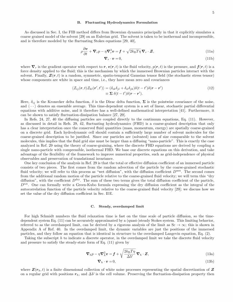
where σij is the average of the diameters of particles i and j, and in this work we set ξij = ξ for all pairs of ions.Note that the repulsion diameter is distinct from the hydrodynamic radius at discussed in Sec. II E, however, both arerelated to the solvation layer formed around an ion [50]. The potential and repulsive force are illustrated in Fig. 1.

11

6

8

4

0.6 0.7 1.00.90.8 1.1 0.6 0.7 1.00.90.8 1.1

4

3

2

2

1

00

FIG. 1. Illustration of short range potential and repulsive force due to Eq. (42). For ease of viewing, here we have set xm = 0.7σ.Note that the actual value used in the simulations, discussed in Sec. V, is xm = 0.25σ.

IV. DETAILS OF NUMERICAL METHODOLOGY

In this section we discuss the details of the discretization and solution methods of the hydrodynamic and electro-static5 equations, Eqs. (13) and (32), and the associated particle time stepping algorithm. These are all implementedin the AMReX framework described in Ref. 51 and available at https://amrex-codes.github.io/.

A. Peskin Kernels

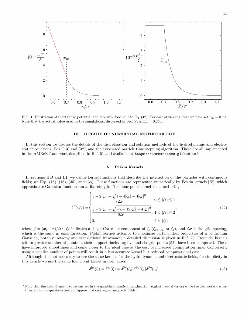
In sections II B and III, we define kernel functions that describe the interaction of the particles with continuousfields; see Eqs. (15), (16), (35), and (36). These functions are represented numerically by Peskin kernels [25], whichapproximate Gaussian functions on a discrete grid. The four-point kernel is defined using

δPe(ζk) =

3− 2|ζk|+√

1 + 4|ζk| − 4|ζk|2

8∆r , 0 ≤ |ζk| ≤ 1

5− 2|ζk| −√−7 + 12|ζk| − 4|ζk|2

8∆r , 1 < |ζk| ≤ 2

0, 2 < |ζk|

, (44)

where ζ = (xi − r)/∆r, ζk indicates a single Cartesian component of ζ, (ζx, ζy, or ζz), and ∆r is the grid spacing,which is the same in each direction. Peskin kernels attempt to maximize certain ideal properties of a continuumGaussian, notably isotropy and translational invariance; a detailed discussion is given in Ref. 25. Recently kernelswith a greater number of points in their support, including five and six grid points [52], have been computed. Thesehave improved smoothness and come closer to the ideal case at the cost of increased computation time. Conversely,using a smaller number of points will result in a less accurate kernel but reduced computational cost.

Although it is not necessary to use the same kernels for the hydrodynamic and electrostatic fields, for simplicity inthis article we use the same four point kernel in both cases,

δhy(ζ) = δes(ζ) = δPe(ζx)δPe(ζy)δPe(ζz). (45)

5 Note that the hydrodynamic equations are in the quasi-hydrostatic approximation (neglect inertial terms) while the electrostatic equa-tions are in the quasi-electrostatic approximation (neglect magnetic fields).

12

We further use the same cell size, ∆r for all fields, although again this is not a necessity.The discretized interpolation operation for a single Cartesian component of the hydrodynamic velocity (vk) is

J hyh,k(xi)vk = ∆V

∑j∈ΩPe

i

δhy(xi − rj)vk(rj), (46)

where ∆V = (∆r)3, and j ∈ ΩPei indicates summation over discrete grid points rj that lie within the support of

δhy(xi − rj) centered on xi, and on which the discrete velocity is defined. The spreading operation for a singlecomponent of force is given by

Shyh (xi)F k =

N∑i=1

∑j∈ΩPe

i

δhy(xi − rj)Fi,k. (47)

Similarly, the discretized electrostatic interpolation and spreading operators are, respectively,

J esh,k(xi)Ek = ∆V

∑j∈ΩPe

i

δes(xi − rj)Ek(rj), (48)

and

Sesh (xi)q =

N∑i=1

∑j∈ΩPe

i

δes(xi − rj)qi. (49)

As mentioned above, one reason for using Peskin kernels is to maximize translational invariance. However asmall degree of variance remains – the four point kernel used here has a position dependent hydrodynamic radiusof (1.255 ± 0.005)∆r. Were perfect translational invariance achieved, for unbounded/triply periodic domains thestochastic drift term in the particle equation of motion, Eqs. (17) and (19), would be zero everywhere, as the divergenceof the mobility would be zero [40]. However the slight lack of invariance of the kernels renders the stochastic driftterm necessary even in domains without solid boundaries; this is discussed in detail in Ref. 24.

B. Fluid solver

We discretize the fluid velocity on a uniform Cartesian grid with mesh spacing ∆r. We use a staggered grid systemwith normal velocities and force density defined at cell faces, and pressure defined in cell centers, i.e., a standardmarker-and-cell (MAC) discretization [53]. Multiple discretizations are used for differential operators representing the

gradient, divergence, and Laplacian. Each of these operators use centered second-order differences. We use ∇c→fh to

represent the face-centered gradient of a cell-centered field, ∇ch to represent the cell-centered gradient of a cell-centered

field, ∇f→ch · to represent the cell-centered divergence of a face-centered field, (∇2

h)f to represent the face-centered

Laplacian of a face-centered field, and (∇2h)c to represent the cell-centered Laplacian of a cell-centered field. Finally,

∇h· is used to represent the face-centered divergence of a field defined on control volumes corresponding to the shifted(staggered) velocity grid. This is illustrated in two dimensions in Fig. 2. Using these operators, the discrete fluidequation solved at each time step is (see Eqs. (13) and (25)),

−η(∇2h)fv + ∇c→f

h p = Shyh F +

√2ηkBT

∆t∆V∇h · Z +

[Shyh

(x+

∆R

2W

)− Shy

h

(x− ∆R

2W

)]kBT

∆RW , (50a)

∇f→ch · v = 0. (50b)

Here, Z represents Gaussian random numbers of mean zero and variance one, defined such that their divergence can

be calculated at the locations where v is defined. This is illustrated in two dimensions in Fig. 2, where Z is stored on

cell nodes and centers. In three dimensions Z is stored on cell edges and centers. This is described in detail in Ref. 26.

The vector W =W 1, · · · , W i, · · · , WN

consists of independent random vectors W i =

(Wi,x, Wi,y, Wi,z

), where

each W is an independent Gaussian random number of mean zero and variance one.

13

FIG. 2. Left: A 2D illustration of the MAC [53] discretization used for Eq. (50). Right: 2D illustration of the ∇h ·Z term inEq. (50a), which is the discretization of the term ∇r · Z from Eq. (11). Random numbers, Z, are generated at the faces ofcontrol volumes around the points where velocities v are defined so that the divergence of the field Z can be calculated.

The second line of Eq. (50a) represents the thermal forcing term given by Eq. (24). As discussed in Ref. 24, itis essentially a finite difference representation of the divergence of the spreading operator. It is implemented by

spreading a random force, kBTW /∆R, at locations randomly offset from the particle positions, x + ∆RW /2, and

the negative of that force at positions x −∆RW /2. The distance ∆R should be smaller than the length scale over

which Shy varies, but large enough to avoid issues due to numerical roundoff. In this article we have used the value∆R = 10−4∆r.

The system of discrete equations formed by Eq. (50) can be solved by a range of approaches, here we have used apreconditioned Generalized Minimal RESidual (GMRES) method [53, 54].

C. Electrostatic solver

The electrostatic potential and charge density, φ and %, are defined on a cell centered grid. The Poisson equation,Eq. (32), is discretized by

(∇2h)cφ = −%/ε. (51)

In this case, the resulting system of equations are solved using the geometric multigrid [55] method.The resulting electric field is also stored at cell centers, and is found by

E = −∇chφ. (52)

The choice of a cell centered differencing in Eq. (52) has some advantages over other options that are worth noting.Importantly, it can be shown6 that Eq. (52), together with the IB interpolation and spreading, ensures that, at leastfor periodic domains, Newton’s third law is obeyed. That is, the force on ion i due to ion j is equal and opposite tothat on ion j due to ion i,7 and momentum is conserved.8 This implies that there is strictly no self-force of one ionon itself, which is an important property desirable in any P3M method. It may appear more natural for staggered

6 We thank Charles Peskin for sharing with us an analytical proof of this property.7 Note that this force is, however, not strictly central. That is, the Weak Law of Action and Reaction (Newton’s Third Law) is obeyed

but not the Strong Law of Action and Reaction, which requires that the forces act along the line joining the particles.8 Note that in the overdamped limit there is no momentum conservation per se, however, the steady Stokes equation would not be solvable

in triply-periodic domains if the forces did not sum to zero.

14

grids to compute electric field not at cell centers using ∇ch, but on cell faces using ∇c→f

h , in particular because

(∇2h)c = ∇f→c

h ·∇c→fh . However, this choice does not lead to equal and opposite action/reaction forces and can

generate spurious self-forces.One thing that is lost with the discretisation employed in Eq. (52) is that the force is no longer a negative gradient

of an electrostatic potential. That is, the IB-P3M approach followed here cannot be used for applications where bothforces and energies matter and need to be consistent with each other; in BD or DISCOS we only need forces, andsince the system is isothermal there are no issues regarding energy conservation. It is possible to ensure consistencybetween electrostatic forces and energy if one uses the derivative of the Peskin kernel to interpolate −φ at the particlepositions to obtain the electric field/force. However, this requires using a smoothly-differentiable kernel such as the6pt Peskin kernel [52], and also does not lead to momentum conservation.

When applying the close range correction to the electrostatic solution (and the steric repulsion), near linear scalingis maintained by using the neighbor list feature included with AMReX.

D. Temporal Algorithm

The time stepping scheme employed in DISCOS builds on that of the FIB method with the addition of electrostaticforces and dry diffusion. A time step is then defined by the following four steps:

1. The charge density % is computed on the grid using the spreading operation defined by Eqs. (36) and (49).Equation (51) is then solved using the geometric multigrid method, and Eq. (52) used to obtain the coarseelectric field, E.

2. This electric field is interpolated to the particle locations using the operation defined by Eqs. (35) and (48). Thecorresponding force on the particles is found using Eq. (37). For particles at close range, this force is correctedas per Eqs. (38) and (39). Close range WCA interactions are also calculated in this step, and the total force onthe particle calculated as per Eqs. (31)-(43), including the effect of any external fields.

3. The force on the particles, F , is spread to the grid storing the force density using the operations defined inEqs. (16) and (47), recovering f s. The random finite difference term is spread as per the second line of Eq. (50a),

yielding the thermal forcing f th. The resulting system, Eq. (50), is solved via the GMRES method to computethe velocity at time step n, vn.

4. The fluid velocity vn is interpolated to particle locations using the operations defined in Eqs. (15) and (46)to obtain the “wet” component of the particle velocities, Eq. (17). The temporal discretization of the particlediffusion is then given by the midpoint update scheme

xn+1/2,?i = xni +

∆t

2(J hy

h (xni )vn), (53)

xn+1i = xni + ∆t

[J hyh (x

n+1/2,?i )vn +

Ddryi

kBTF ni +

√2Ddry

i

∆tW n

i

. (54)

As discussed in Sec. II B, the purpose of the midpoint update is to incorporate the part of the stochastic driftnot accounted for by the random finite difference force density f th.

This algorithm is first order in time, as illustrated in Ref. 24, where higher order schemes are also discussed.

V. NUMERICAL RESULTS

In this section we test the DISCOS algorithm by comparison with theoretical results for the radial pair correlationfunction and electrical conductivity. Additionally, we analyze the effect of changing the ratio of wet and dry diffusion.

In our numerical tests we model a 1:1 strong electrolyte solution, similar to salt water, with species labeled A and B,with charges q = qA = −qB = 1.6×10−19 C. The solvent is taken to be water at T = 295 K, viscosity η = 0.01 g/(cm s),and permittivity ε = εrε0, with relative permittivity εr = 78.3 where ε0 is the vacuum permittivity. The diffusioncoefficients of the ions in water are Dtot

A = 1.17 × 10−5 cm2/s and DtotB = 1.33 × 10−5 cm2/s, corresponding to

hydrodynamic radii of at = 0.185 nm, and at = 0.162 nm, respectively. In all cases the close range potentialparameters are ξ = 10−16 ergs, σ = 0.4 nm, and xm = 0.1 nm. Note that the above parameters yield Schmidt

15

numbers of 854 and 752 for species A and B, respectively. This justifies the use of the infinite Schmidt numberapproximation discussed above.

For each problem the time step, ∆t, was selected by successive refinement until a negligible change in the resultwas observed. Note that the ion diffusive time scale, a2

t/D, is on the order of 10 picoseconds. The time steps used forthe simulations below were typically constrained to the order of 0.1 ps by the stiffness of the steric and electrostaticinteractions. We are currently examining how the time step may be increased by varying the parameters of thesepotentials.

In each case the system size was selected to avoid significant finite size effects. When considering electrostaticinteractions, the relevant length scale is the Debye length [56, 57],

λD =

√εkBT∑Ns

j=1 njq2j

, (55)

where Ns it the number of species, and nj is the number density of species j. This is a measure of how far electrostaticeffects persist before they are screened by clouds of opposite charges. For hydrodynamic effects, it should be noted thatthe diffusion coefficient of an isolated particle in a triply-periodic domain has well-known strong finite-size correctionsof order aw/L [43], where L is the length of the cubic domain. This is because the mobility of an isolated particle isdetermined by applying a force on it, and a force monopole interacts with its periodic images with 1/r hydrodynamicinteractions. However each ion diffuses with its Debye cloud, which experiences an equal but opposite force, so thatan ion interacts with its periodic images hydrodynamically as a force dipole [58], which has a finite size correctionof order (aw/L)3. We are not aware of any systematic analysis of finite-size effects in the literature; here we havesystematically increased the system size until no significant change in the result is observed.

A. Radial Pair Correlation Function

We first validate the equilibrium properties of the DISCOS method by measuring radial pair correlation functionsbetween ions of like and opposite charge. In general, the radial pair correlation function is the normalized time-average density of particles as a function of radius from an arbitrary reference particle. For a binary system, the paircorrelation function between species α and β is defined as [14]

gαβ(x) = limτ→∞

VNαβ(Nαβ − 1)4πx2τ

∫ τ

0

N∑i,j,i 6=j

δ(x− xij) δα,siδβ,sjdt, (56)

where V is the system volume, si and sj are the species of particles i and j, Nαβ is the number of species pairs, andxij is the radial distance between particles i and j. In practice, for each snapshot in time, for each ion of type α, wecount the number of ions of type β in thin spherical shells with a specified bin width, and compute a number densityin each bin by dividing by the volume of the shell. We average the results over all α ions and over many time steps,and normalize the result with the average number density of β.

For low to moderate ion concentrations Debye-Huckel theory [56, 57] gives

gαβ(x) ≈ exp(−Uαβ(x)/kBT ), (57)

where the potential is

Uαβ(x) =qαqβ4πε

e−x/λD

x+ U sr

αβ(x). (58)

The first term in Eq. (58) is the screened Coulomb potential [56, 57] and the second is the short-ranged repulsion.In Figs. 3 and 4, we compare the approximate theoretical expression of Eq. (57) with results obtained from DISCOS.

In Fig. 3, the comparison is shown for molarity (moles of cation or anion per liter of solvent) of 0.1 M; excellentagreement is observed. Fig. 4 shows the comparison for a molarity of 1.0 M for two different ratios of wet and drydiffusion. A negligible difference is observed between second and third simulations; this is unsurprising as we cansee from Eq. (57) that the pair correlation function does not depend on the hydrodynamic properties of the solvent.Reasonable agreement is observed, with the largest deviation observed in the peak of the opposite charge result.We note that Eq. (57) is derived in the low concentration limit so we expect decreasing agreement with increasingconcentration. At the higher concentrations the Percus-Yevick and hypernetted chain (HNC) approximations aremore accurate [59].

16

0.6

0.8

0.4

0.2

0.0

1.0

3.0

4.0

2.0

1.0

0.0

5.0

0 321 4 0 321 4

FIG. 3. Radial distribution for a molarity of 0.1 M. The right plot shows the pair correlation for ions of like charge; alsoindicated is the Debye length. The left plot shows the pair correlation for ions of opposite charge. The solid line shows theapproximate analytical solution given by Eq. (57), and the squares show the numerical result from DISCOS. These results werecollected using a bin width of 0.025 nm, with a sample size of 50,000 – the simulation was run for 100,000 steps, with the first50,000 steps used for equilibration. This sample size resulted in negligible statistical error. For visual clarity, only every fourthpoint is displayed. The grid size was set such that the total diffusion of species A was 14.7% wet and 85.3% dry, and for speciesB, 12.9% wet and 87.1% dry. This corresponds to ∆r = 1nm, with a 32 × 32 × 32 cell periodic domain, and 3946 ions. Thetime step was ∆t = 0.1 ps.

B. Electrical Conductivity

For an applied electric field of magnitude E the total current density in an electrolyte solution is

I =

Ns∑j=1

njq2jµjE, (59)

where µj is the mobility of species j. The conductivity is defined by Ohm’s law as C = I/E and from the Nernst-Einstein relation [57] the mobility in the limit of infinite dilution is µ0

j = Dtotj /kBT . In this limit, the uncorrected

total conductivity C0 is the sum of the species conductivities C0i ,

C0 =

Ns∑j=1

C0j =

Ns∑j=1

njq2jD

totj

kBT. (60)

Debye-Huckel-Onsager (DHO) theory gives the electrolyte conductivity [57, 60] as the sum of the uncorrected totalconductivity, electrophoretic contribution, and a contribution due to the relaxation effect,

C = C0 + Cep + Crelx. (61)

See Ref. 12 for the relationship of this theory to fluctuating hydrodynamics.The electrophoretic contribution is due to screening charges of opposite sign about each ion imparting a retarding

viscous stress on the ion, given by

Cep = −Ns∑j=1

njq2j

6πηρλD

λDλD + aDH

j

. (62)

17

0.6

0.8

0.4

0.2

0.0

1.0

1.5

2.0

1.0

0.5

0.0

2.5

0 21 0 21

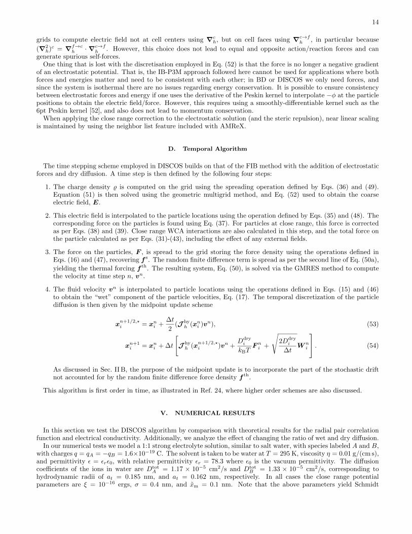
FIG. 4. Radial distribution for a molarity of 1.0M. The right plot shows the pair correlation for ions of like charge; also indicatedis the Debye length. The left plot shows the pair correlation for ions of opposite charge. The solid line shows the approximateanalytical solution given by Eq. (57), and the boxes and circles show numerical result from DISCOS. The numerical parametersare the same as those described for Fig. 3, except that two different grid resolutions are shown. The black circles show thecase where the grid size was set such that the total diffusion of species A was 14.7% wet and 85.3% dry, and for species B,12.9% wet and 87.1% dry. This corresponds to ∆r = 1nm, with a 16 × 16 × 16 cell periodic domain, and 4932 ions. The redsquares show the case where the grid size was set such that the total diffusion of species A was 58.9% wet and 41.1% dry, andfor species B, 51.8% wet and 49.2% dry. This corresponds to ∆r = 0.25nm, with a 32 × 32 × 32 cell periodic domain, and 618ions.

The last term is a Debye-Huckel correction to account for the finite ion size, which we take to be aDHj = 0.4 nm for

both ions. The relaxation effect refers to the average force experienced by an ion from its asymmetric ionic cloudrelaxing due to thermal fluctuations. For binary electrolytes the contribution due to the relaxation effect is

Crelx = −2∑j=1

C0

12π(2 +√

2)

q2j

εkBTλD

λDλD + aDH

j

. (63)

For aDHj λD both the electrophoretic and relaxation contributions go as the square root of the ionic concentration.

The C0 term contains no hydrodynamic interactions between ions; it is therefore correctly captured by a simulationwith any wet/dry diffusion ratio. The same is true for the Crelx term, as this arises entirely from electrostaticinteractions which are well-resolved using the P3M approach. The Cep term arises from the collective hydrodynamiceffect of an ion and its screening cloud of opposite charge, it is therefore only completely captured by a simulationusing 100% wet diffusion; the relative importance of this effect is discussed in the next section.

When the applied electric field is sufficiently strong the distortion of the ionic clouds results in an increased electricalconductivity, which is known as the first9 Wien effect. For a 1:1 strong electrolyte solution the Wien corrections tothe conductivity are [61]

CrelxW (a) = AW(a) Crelx, (64)

CepW(a) = BW(a) Cep, (65)

where

AW(a) =3(1 +

√1/2)

2a3

(a√

1 + a2 −√

2a + arctan(√

2a)− arctan(a/√

1 + a2)), (66)

9 Note that there is a “second Wien effect” which applies to weak electrolytes.

18

BW(a) =1√2

+3

8a3

(2a2arcsinh(a)− a

√1 + a2 +

√2a −(1 + 2a2)

[arctan(

√2a)− arctan(a/

√1 + a2)

] ), (67)

and a = (qλDE)/(kBT ) is a dimensionless parameter for the electric field strength. These correction factors are shown

in Fig. 5. Note that AW(a)→ 0 and BW(a)→ 1/√

2 as a→∞.

0.6

0.8

0.4

0.2

0.0

1.0

0 302010 40

FIG. 5. Wien corrections to the DHO relaxation effect and electrophoretic contribution as a function of a = (qλDE)/(kBT ).

In the presence of an applied electric field, the conductivity vector can be computed by

C = limτ→∞

1

EVτ[Z(τ)− Z(0)] , (68)

where the ion polarization (displacement of the “center of charge”) is

Z(t) =

N∑i=1

qixi(t). (69)

An alternative way to measure conductivity in the absence of an applied field is given by the Einstein-Helfandformula [62], in terms of the long-time diffusion coefficient of the center of charge,

CEH = limτ→∞

1

6kBTVτ

∫ τ

0

[Z(t)− Z(0)]2dt. (70)

This is derived from the Green-Kubo relation [63, 64], and is discussed in Refs. 62 and 65.Formally, Eqs. (68) and (70) hold when τ is large enough to ensure that the short time correlations have decayed;

increasing τ beyond this point has no effect on the statistical convergence, as the variance of Z does not decrease withtime. An accurate result can be obtained by increasing N , or averaging an ensemble of simulations. We find thatthe mean-square displacement of the center of charge is perfectly linear in time on our overdamped time scales for allτ examined, so the conductivity is not sensitive to the choice of τ . The correct result can therefore be obtained bysetting τ ∼ ∆t to maximize the statistical sample size. To ensure de-correlation between simulation measurementsthe conductivity was sampled at intervals of 10 ps, which is on the order of the ion diffusion time, when calculatingthe time average in Eq. (68). For Eq. (70), the displacement in Z was measured and then reset every 10 ps. Notethat this has no impact on the result itself, but it influences the calculation of the statistical error.

Three sets of conductivity simulation measurements were performed at a concentration of 0.1 M: (i) Measurementswith zero applied field using Eq. (70), (ii) using a weak applied field of 105 V/cm (a = 0.377), and (iii) using a strongapplied field with a value of 107 V/cm (a = 37.7), each using Eq. (68). In each case a range of diffusion ratios,

19

i.e. values of Dwet and Ddry, were tested. Tests using case (i) with Eq. (70) were also performed at concentrations of0.0115 M, 0.5 M, and 2 M. The results are summarized in Table I and illustrated in Fig. 6.

All simulations were performed in a cubic domain with length L = 10.043 nm. For concentrations 0.0115 M, 0.1 M,0.5 M, and 2 M, the domain contained 14, 122, 610, and 2440 ions, respectively. For comparison, a molecular dynamicssimulation of this system would contain roughly 30,000 water molecules.

To vary the wetness, the computational domain was divided into 83, 163, 323, or 643 grid cells for both the Stokesand Poisson solvers; simulations with fully dry diffusion used a 323 grid for the Poisson solver. The 83 grid cell casescorrespond to wetness percentages of 11.8% and 10.3% for ion A and B, respectively, while the 643 grid cell casescorrespond to wetness percentages of 93.8% and 82.6%. Most simulations for molar concentrations of 0.5 M and belowused a time step size of 0.1 ps, while for the high molarity 2 M cases ∆t was typically between 0.01 and 0.02 ps.It is important to note that while a Stokes grid as coarse as 83 does little to accelerate the far-field calculations fornearest image particles, the use of a periodic Stokes solver is crucial to account for the hydrodynamic interactionswith periodic image particles; the same applies also to the Poisson solver.

In all cases, good agreement is observed between the results with the highest Dwet value and the theoreticalprediction, for both high and low field cases, and at all concentrations. The weak and strong field results are inparticularly good agreement with the theory for both fully dry and fully wet simulations. Note that DHO theory maynot be accurate at high molarities, especially since we do not tune the value of the finite-size radius aDH for eitherspecies. The dry (Dwet=0) cases also compare reasonably well with the theoretical result with the electrophoreticcomponent removed, in agreement with the discussion above.

For the weak field simulations, the strength of the field has been set such that the Wien effect is negligible; wetherefore expect the same results for the weak and zero field cases. Interestingly, a difference of about 3% is observedfor the highest wet percentage, and 5% for the lowest. The cause of this discrepancy is not apparent, but warrantsfurther investigation.

Measured in case wet% A, wet% BTheory 0% 11.75% 23.5% 46.9% 93.8% TheoryNo EP 0% 10.33% 20.65% 41.3% 82.6% With EP

Zero E-field0.01147 M 0.106 0.1086(18) 0.1013(6) 0.1020(21) 0.1002(21) 0.1010(18) 0.1000.1 M 0.897 0.946(12) 0.869(27) 0.837(21) 0.813(9) 0.803(12) 0.7760.5 M 4.33 4.70(6) 4.21(9) 3.95(6) 3.63(6) 3.54(15) 3.342 M 16.8 18.5(6) 16.7(9) 14.8(9) 12.8(6) 11.6(9) 11.4

Weak E-field0.1 M 0.897 0.898(6) 0.831(6) 0.785(6) 0.785(9) 0.777(6) 0.776

Strong E-field0.1 M 0.943 0.943(3) 0.870(3) 0.851(3) 0.841(3) 0.837(3) 0.850

TABLE I. Conductivity simulation measurements in siemens per meter for zero E-field (by Einstein-Helfand, Eq. (70)) andweak and strong E-field (center of charge displacement, Eq. (68)). The uncertainty notation is defined such that the numbers inparenthesis indicates the error bar for the final digits, e.g., 0.898(6) indicates 0.898±0.006, and 0.946(12) indicates 0.946±0.012.The right column is calculated from DHO theory including Wien effect corrections for the strong E-field cases. For comparisonwith the 0% wet case, the theory prediction without the electrophoretic (EP) correction is also included in the table. A plot ofthese results is given in Fig. 6.

C. Effect of wet vs. dry diffusion

The results in the previous section show that while some wet diffusion is needed to capture the electrophoreticcontribution to conductivity, in most cases increasing the wet diffusion above 50% has a relatively small impact. Fur-thermore the relative effect depends on concentration, with wet diffusion making a greater contribution at higher molarconcentrations; this can be clearly seen in Fig. 6. As mentioned in Sec. II E, reducing the hydrodynamic resolution(by reducing Dwet) neglects short range hydrodynamic interactions. It seems clear that short range hydrodynamicinteractions should increase in importance as concentration increases, i.e., as the particles are on average closer to-gether. However it must be noted that this will also increase the relative importance of electrostatic interactions,which decay more rapidly than hydrodynamic influence.

To estimate the importance of these effects, and obtain an estimate for the required Dwet value for a given con-centration, we consider two ions, 1 and 2. In Fig. 7, the effect of dry diffusion on the particle mobility matrix is

20

0.4

0.6

0.2

0.0

0 20 806040

FIG. 6. Relative difference in conductivity from DHO theory including Wien corrections for the strong field case), as a functionof wetness percentage, for a range of molarities; based on data from Table I.

illustrated as a function of particle separation. The mobility parallel and perpendicular to the vector connecting theparticles is shown, measured from 100% wet and 50% wet simulations. These are compared to the solution obtainedfrom the RPY tensor, Eq. (7). As discussed above, increasing the percentage of dry diffusion amounts to neglectingshort range hydrodynamic interactions; as per Eqs. (26)–(30), changing from 100% wet to 50% wet is equivalent todoubling the hydrodynamic radius.

To represent the dry component of the particle mobility, we introduce the dry tensor

Mdry(a) =1

6πηaI. (71)

The velocity of particle 1 has two contributions: that directly induced by the Coulomb force, Eq. (38),

V dir1 =

(R(0, aw) + Mdry(ad)

)FC

12

= R(0, at)FC12 = Mdry(at)F

C12. (72)

and the disturbance in the fluid induced by particle 2, which is subject to the opposite force,

V dst1 = −R(x21, aw)FC

12, (73)

with the total velocity of particle 1 (parallel to the vector x12) being

V 1 = V dir1 + V dst

1 . (74)

In Fig. 8 we plot V1 as a function of particle separation. Five curves are shown, ranging from 0% to 100% wet,with increments of 25%. Also marked, with vertical lines, are the measured average nearest particle separations fortwo concentrations, 0.1 M (black) and 2 M (red). At 0.1 M varying the wetness from 50-100% produces only a 2%change in particle velocity. At 2 M the same range produces a change in velocity of 33%, suggesting a higher wetnesspercentage is necessary to accurately capture the solution at higher molarities, as expected.

In Fig. 9 particle velocity is shown as a function of wet percentage, for a range of ion separations using the sametwo ion system; the curves are normalized by the value at 0% wet. In addition to the measured nearest ion separation(solid lines), for comparison we have also indicated the average nearest particle distance obtained by assuming theparticles are in a random configuration (dashed lines), and in a cubic lattice (dotted lines). For randomly distributedparticles the average nearest particle distance is [68]

x12 = Γ( 43 )( 4

3πn)−1/3 ≈ 0.55 n−1/3, (75)

21

1.0

0.8

2 864 100

0.6

0.4

0.2

1.0

0.8

0.6

0.4

0.2

2 864 100

FIG. 7. Left: Mobility of particle 1 when a force is applied on particle 2, in the direction parallel to the vector connectingparticles 1 and 2. Right: Mobility of particle 1 when a force is applied on particle 2, in the direction perpendicular to thevector connecting particles 1 and 2. The red circles are values measured from a 100% wet simulation, the black crosses from a50% wet simulation. In each case the values are normalized by the particle self mobility, and the separation is shown in termsof the average particle radius of species A and B, i.e., at = (aAt + aBt )/2, aw = (aAw + aBw)/2, ad = (aAd + aBd )/2. Each set ofdata is compared to the result from the RPY tensor calculated using aw, shown with the red and black solid lines. Also shownfor comparison is the RPY result corresponding to the 75% wet case (dashed line). The approach of using the average particleradius has been used for simplicity because the two species are of similar size; we note that a polydisperse version of the RPYtensor is described in Ref. 66. Simple fits of the pair mobility for the 6-point Peskin kernel is given in Ref. 67.

FIG. 8. Particle velocity due to electrostatic and hydrodynamic interactions between two ions, as a function of separation.The velocity V1 is calculated using Eqs. (72)-(74), using a radius averaged from species A and B, i.e., at = (aAt + aBt )/2,aw = (aAw +aBw)/2, ad = (aAd +aBd )/2. A range of wet percentages are shown, the corresponding particle radii can be found withEqs. (29) and (30) and the radii quoted at the start of Section V. The measured average closest ion separations correspondingto concentrations 0.1 M and 2 M are indicated with the black and red vertical lines.

22

where Γ(x) is the gamma function. Assuming a cubic lattice arrangement gives

x12 = n−1/3. (76)

Also shown are the conductivity simulation measurements from Table I, again normalized by the 0% wet value. Forboth 0.1 M and 2 M the conductivity measurements follow a similar trend to the particle velocity, suggesting thatthe simple particle velocity calculation from Eqs. (72)-(74) is a useful indicator of the lower bound of wet diffusionnecessary to accurately simulate a given molar concentration. For example, the change of 2% in the particle velocityfor the 0.1 M case corresponds to a 1% change in conductivity for the two highest wetness ratios, while the 33%change in velocity for the 2 M case corresponds to a change in conductivity of 10%.

0 20 806040 100

0.8

0.7

0.9

1.00

0.6

0.5

FIG. 9. Normalized particle velocity due to Eq. (74) (lines), and normalized conductivity simulation measurements from Table I(symbols), as a function of wet/dry ratio of species A. All values are normalized by the 0% wet value. Black signifies 0.1 M, red2 M. The curves indicate the particle velocity, calculated at the average nearest particle separation measured from simulation(solid), and corresponding to random (dashed), and cubic lattice (dotted) configurations. Squares are zero-field conductivitymeasurements using the Einstein-Helfand formula (Eq. (70)), diamonds indicate weak-field conductivity measurements usingthe center of charge displacement (Eq. (68)), and crosses are the prediction of DHO theory (Eq. (61)).

VI. CONCLUSIONS

In this article we have presented a new approach for the simulation of electrolytes at the mesoscale. The methodextends the FIB method to include electrostatic interactions, and incorporates a “dry diffusion” process to correctfor under-resolution of the hydrodynamics. The dry diffusion term allows the method to be applied to systems ofelectrolytes where application of the standard FIB approach would require an excessively fine grid to resolve particlesof nanoscopic size. We note that our approach is similar to the Stochastic Eulerian Lagrangian Method [27, 69, 70]and the stochastic Force Coupling Method [44, 71–73]; the relationship of each of these to the FIB method is discussedin Ref. 24. In principle, some of the techniques outlined in this article could also be applied in the context of thesedistinct numerical approaches.

In sections V A and V B, we have demonstrated that the DISCOS method accurately reproduces several importantproperties of electrolytes. In Sec. V C, we have demonstrated that the dry diffusion approach can effectively replaceresolving the near-field hydrodynamics at scales smaller than the typical ion-ion distance. At 0.1 M, reducing thewetness to approximately 50% produces only a 2% change in the conductivity, but at 2 M a 10% change is observed.Dry diffusion can therefore be used to reduce the numerical resolution needed to simulate an electrolyte, but thisapproach becomes less effective as the ion concentration is increased.

Our results clearly demonstrate that, for denser electrolyte solutions, near-field hydrodynamic interactions con-tribute to macroscopic transport properties such as conductivity. As discussed in great detail in Ref. 40, wet diffusion,

23

which is diffusion due to advection by a fluctuating velocity field, and standard dry diffusion, are very different bothphysically and mathematically. This difference cannot be seen for a single particle since ultimately only the total(effective or renormalized) diffusion coefficient matters; it is worth recalling that in Ref. 29 only a single nano-particleis analyzed. The difference between wet and dry diffusion, however, manifests itself in collective properties such asthe spectrum of nonequilibrium concentrations [40]. However, experimentally distinguishing between wet and drydiffusion based on this spectrum requires examining length scales below light-scattering reach, and, at the scales ob-servable in typical experiments, one only sees a total (effective or renormalized) diffusion coefficient. Our work showsthat electrical conductivity, which is easily measured to high accuracy, is a sensitive probe that is affected by thehydrodynamic interactions (equivalently, the spectrum of the fluctuating velocity field [40]) at distances comparableto the typical ion-ion spacing. In the future, it is important to perform more detailed comparisons between simula-tions for different degrees of “wetness” and results for denser electrolytes obtained using experiments or large-scalemolecular dynamics simulations. This will shed light on how good of a model the Rotne-Prager-Yamakawa tensor isfor solvated ions.

A key advantage of the FIB method is the ability to handle other types of boundary conditions, notably confinementby no-slip walls. As the discussion of DISCOS in this context requires considerable exposition, of both details of thealgorithm and the physics that arises, we defer this to a future publication. However, as previously noted, we givesome brief comments in Appendix C. It is perhaps more relevant to contrast the numerical method used in DISCOSto the state-of-the-art Positively Split Ewald (PSE) method for Brownian Dynamics with hydrodynamic interactionsdeveloped in Ref. 21, by using some ideas from spectral Ewald methods for electrostatics [48] combined with theidea of using fluctuating hydrodynamics to generate the far-field Brownian displacements. The PSE method includesa spectrally-accurate implementation of the Hasimoto-Ewald splitting used in GGEM [17]; this splitting allows oneto choose the grid size arbitrarily by using the same idea of local near-field corrections that we used here for thePoisson equation. However, at present, the PSE approach relies on Fourier-space decompositions and using theFFT algorithm, and therefore only apply to triply-periodic domains. It remains a future challenge to find a way toincorporate near-field hydrodynamic corrections to correct for under-resolution of the hydrodynamics by the Stokessolver used in FIB and DISCOS, while also computing Brownian motion without expensive iterations.

In future work we intend to apply DISCOS to strong electrolyte solutions that are acids (e.g., HCl) or bases (e.g.,NaOH) instead of salts. Also of interest are solutions in which the Wien effect is more pronounced, such as weakelectrolyte acids and bases (e.g., acetic acid, ammonium hydroxide) and strong electrolyte salts that are not 1:1 (e.g.,MgCl2). Furthermore, recent work suggests that non-aqueous solvents with low permittivity (e.g., benzene) exhibitunusual Wien effects [74].

Here we have described the DISCOS approach for simple mono-atomic, 1:1 electrolytes, where each ion is describedby a single IB kernel. In principle, multiple kernels may be combined to form complex molecules such as chargedpolymers or DNA strands. This approach has already been tested in the context of BD, for example in Refs. 30 and31, and for electrically neutral systems using FIB, for example in Refs. 67, 75, 76. Future work may also include theextension of DISCOS to encompass these cases. Further, there is the possibility of simulating large molecules, suchas DNA, in a solution represented as a continuum that includes smaller ionic species. This was done previously usinga deterministic solution in Ref. 77, in this case the solution would be modeled using the fluctuating hydrodynamicapproaches outlined in Refs. 11–13.

ACKNOWLEDGEMENTS

The authors thank Changho Kim for discussions regarding electrolyte chemistry, and Charles Peskin and JonathanGoodman for discussions regarding the IB-P3M method. This work was supported by the U.S. Department of Energy,Office of Science, Office of Advanced Scientific Computing Research, Applied Mathematics Program under contractNo. DE-AC02-05CH11231. This research used resources of the National Energy Research Scientific Computing Center,a DOE Office of Science User Facility supported by the Office of Science of the U.S. Department of Energy underContract No. DE-AC02-05CH11231. A. Donev was supported in part by the Division of Chemical, Bioengineering,Environmental and Transport Systems of the National Science Foundation under award CBET-1804940.

Appendix A: Accuracy of immersed-boundary P3M solver

In this appendix we examine the accuracy of the immersed-boundary P3M method described in Sections III Aand IV C. In particular, we focus on the degree of translational and rotational invariance of the electrostatic forcescomputed by the method for a pair of ions of equal and opposite charge qi = −qj at a distance r from each other,using a uniform regular grid of spacing ∆r. The periodic box size L r so that periodic effects can be neglected.

24

We include in our tests both the 4-point (see Eq. (44)) and 6-point [52] Peskin kernels, given by

δPe(ζk) =

0, ζk ≤ −3

ϕ(ζk), −3 < ζk ≤ −2

−3ϕ(ζk)− 116 +

K + ζ2k

8 +(3K − 1)ζk

12 +ζ3k12 , −2 < ζk ≤ −1

2ϕ(ζk) + 14 +

(4− 3K)ζk6 − ζ3

k6 , −1 < ζk ≤ 0

2ϕ(ζk) + 58 −

K + ζ2k

4 , 0 < ζk ≤ 1

−3ϕ(ζk) + 14 −

(4− 3K)ζk6 +

ζ3k6 , 1 < ζk ≤ 2

ϕ(ζk)− 116 +

K + ζ2k

8 − (3K − 1)ζk12 − ζ3

k12 , 2 < ζk ≤ 3

0, 3 < ζk

, (A1)

where

ϕ(ζk) =

(−ϑ(ζk) + sgn

(3

2−K

)√ϑ2(ζk)− 112ς(ζ)

)/56,

ϑ(ζk) = 9/4− (3/2)(K + ζ2k)ζk + (22/3− 7K)ζk − (7/3)ζ3

k ,

ς(ζk) = −(11/32)ζ2k + (3/32)(2K + ζ2

k)ζ2k + (1/72)

((3K − 1)ζk + ζ3

k

)2+ (1/18)

((4− 3K)ζk − ζ3

k

)2,

K = 59/60−√

29/20.

In order to compare to alternative methods, these tests were performed in Matlab using FFTs instead of multigrid tosolve the (discrete) Poisson equation. In addition to the 2nd-order electrostatic solver based on the 7-point Laplacian(∇2

h)c and centered difference ∇ch, we also include, for comparison, results obtained by using a fourth-order compact

isotropic 24-point Laplacian in Eq. (51) and a 4-point centered difference in Eq. (52).In addition to the fourth-order finite-difference Poisson solver, we also implement a spectral Fourier solver, as used

in the Spectral Ewald (SE) method [48]. As explained in Section III A, the SE approach (and essentially all otherEwald methods) uses a Gaussian of standard deviation σ as the kernel δes in Eqs. (35) and (36). This allows oneto compute the electrostatic force between the two Gaussian charge clouds analytically for an unbounded domain,10

giving the required local correction

FLCGaussian =

(∆r

r

)2(erfc

( r

2σ

)+

r

σ√π

exp

(− r2

4σ2

))(A2)

that decays exponentially with distance. However, achieving 3-4 digits of accuracy with Gaussian kernels requiresthe support of the kernel to be on the order of 10-12 grid points in each dimension, which is expensive. Therefore,to make a more fair comparison with the 6-point Peskin kernel, here we couple the spectral Poisson solver with arecently-developed “exponential of a semicircle” (ES) kernel [78] with width w = 6; we optimized the value of theparameter β = 1.8w for translational and rotational invariance.11

Fig. 10 shows numerical data for the radial component of the near-field correction to the electrostatic force F LCij

for several kernels and Poisson solvers, expressed in terms of the dimensionless function FLC(x = r/∆r) appearing inEq. (41). To quantify the loss of translational and rotational invariance, we randomly generate the position of many

pairs of particles at a distance r from each other. Note that if F LCij were purely radial and its magnitude were purely

a function of r, the local-correction approach used here could completely correct the electrostatic force computed bythe discrete solver to match the Coulomb force between point charges. Therefore, the main cause of inaccuracy isthe loss of translational and rotational invariance. In Fig. 10 we also show the correction FLC(x = r/∆r) for a pairof Gaussian charge clouds given in Eq. (A2). The value of the Gaussian width σ was fitted to match the numericalresults over the range 0 < x < 3, giving σ ≈ 0.78∆r for the 4-point and σ ≈ 0.89∆r for the 6-point Peskin kernels

10 Note that the periodic boundaries are implemented by using a Fourier series instead of a Fourier sum.11 We point out again that this approach, while similar to the Spectral Ewald method [48] based on the non-uniform FFT [78] using the

ES kernel, is different because we do use the same kernel to both smear the charges and to communicate to the grid, rather than usingtwo different kernel functions (Gaussian for smearing and ES for grid transfers in the NUFFT).

25

1 2 3 4 5 6 7

x = r/∆r

10-5

10-4

10-3

10-2

10-1

100

101

Co

rrec

tio

n

FL

C(x

)

4pt Peskin IB-P3M

Empirical mean

Gaussian σ=0.78 ∆r

1 2 3 4 5 6x = r/∆r

10-5

10-4

10-3

10-2

10-1

100

101

Co

rrec

tio

n

FL

C(x

)

6pt Peskin IB-P3M

Gaussian σ=0.89 ∆r6pt ES spectral

FIG. 10. Local correction function FLC(x = r/∆r) computed from the radial component of the near-field correction to theelectrostatic force, F LC

ij , for the Peskin 4pt kernel (top panel) and the Peskin 6pt kernel (bottom panel). Red circles are samplesfor different positions and orientations of the pair of ions, while dashed blue lines indicate the continuum theoretical near-fieldcorrection FLC

Gaussian for Gaussian charges of standard deviation σ indicated in the legend (see Eq. (A2)). The black solid linein the top panel indicates the empirical mean used to tabulate FLC in our method. The bottom panel includes results (blacksquares) for a spectral Poisson solver with a 6-point exponential of a semicircle (ES) kernel [78] with parameter β = 1.8 × 6.

with the 2nd order Poisson solver. This can be thought of as an effective width of the charges similar to the effectivehydrodynamic radius aw for Stokes flow.

The spread in the symbols in Fig. 10 shows the loss of translational and rotational invariance. We see in the toppanel that the mean correction force decays algebraically rather than exponentially as it does for Gaussian charges.We also see that the 6pt kernel improves the invariance, especially at short distances. Using a fourth-order isotropicPoisson solver further improves the invariance for all distances (data not shown in Fig. 10), as does using a spectralPoisson solver with the 6-point ES kernel, as shown in the bottom panel of Fig. 10. For the 4-point kernel, we seein the top panel of the figure that truncating the local corrections for pairs of particles further than 3-grid pointsapart, ψ = 3∆r, makes the error due to loss of invariance dominate the error due to truncation of FLC(x = r/∆r),and therefore there is no point in further increasing the cutoff distance ψ; similarly, for the 6-point kernel ψ = 4∆ris suitable.

We further quantify the amount of translational and rotational variance in Fig. 11. The top panel shows the spreadin the symbols in Fig. 10 for each distance r, measured as two standard deviations of the samples. We normalizethe spread by 1/x2 to obtain a measure of the invariance of the radial component of the electrostatic force relativeto the true Coulomb potential, and express the error in percent; note that this is the error in the final answer forthe electrostatic force between two ions. The bottom panel shows the magnitude of the non-radial component of theelectrostatic force computed by the Poisson solver, FP

ij , relative to it’s radial component, again expressed as percenterror. The top panel of Fig. 11 shows that the second-order Poisson solver is translationally and rotationally invariantto about 8% for the 4-point kernel and about 6% for the 6-point Peskin kernel, with the 6-point kernel being notablymore accurate at short distances. The fact that errors become comparable for large distances regardless of the widthof the kernel suggests that for large distances the error is dominated by the anisotropy of the discrete Green’s functionfor the standard 7-point Laplacian. Switching to a fourth-order Laplacian drops the maximum error down to 2% forthe 6-point kernel, while the spectral solver with the 6-point ES kernel drops the error below 0.5%. The bottom panelof the figure shows that all combinations of kernels and solvers studied here achieve a central electrostatic force towithin 1.5%, which is remarkably good.

Appendix B: P3M correction tables

The numerical results in the main body of this work were computed using a four-point Peskin kernel [25], additionalanalysis in Appendix A uses a six-point kernel [52]. As per Eqs. (40) and (41), the P3M procedure uses pre-computedtables to apply a near field correction to electrostatic forces. The values for each kernel are given below in Table II.Note that for values of FP between the tabulated positions linear interpolation was used.

26

0 1 2 3 4 5 6 7r / ∆r

0.01

0.1

1

10%

er

ror

du

e to

in

var

ian

ce

4pt Peskin, 2nd order

6pt Peskin, 2nd order

6pt Peskin, 4th order

6pt ES, spectral

0 1 2 3 4 5 6 7

r / ∆r

0

0.5

1

1.5

% ce

ntr

alit

y

4pt Peskin, 2nd order

6pt Peskin, 2nd order

6pt Peskin, 4th order

6pt ES, spectral

FIG. 11. Percent error due to loss of translational and rotational invariance in the immersed-boundary P3M method based ondata shown in Fig. 10. In addition to the method used in this work, we include for comparison the improvement gained by usinga fourth-order isotropic Poisson solver, as well as a spectral Poisson solver with a 6-point ES kernel. (Left) Percent error in theradial component of the total electrostatic force due to loss of invariance. (Right) Magnitude of the non-radial component ofthe IB force FP expressed as percent of the radial component. The symbols show the empirical mean over samples of pairs ofpoints, while the dashed lines show the maximum value over the samples.

four-point six-point four-point six-point four-point six-point six-pointxij∆r FP

(xij∆r

)FP(xij∆r

)xij∆r FP

(xij∆r

)FP(xij∆r

)xij∆r FP

(xij∆r

)FP(xij∆r

)xij∆r FP

(xij∆r

)0 0 0 2.0 0.165755 0.133308 4.0 0.0627171 0.0616157 6.0 0.0275866

0.1 0.0191993 0.0130335 2.1 0.162663 0.130995 4.1 0.0591556 0.0586423 6.1 0.02676070.2 0.0384104 0.0259347 2.2 0.156037 0.129343 4.2 0.0561682 0.0561644 6.2 0.02593470.3 0.0561438 0.0384891 2.3 0.148626 0.126205 4.3 0.0539003 0.0535214 6.3 0.02510880.4 0.0745141 0.0507132 2.4 0.144648 0.122075 4.4 0.0511791 0.0513739 6.4 0.02428290.5 0.0914394 0.0624416 2.5 0.138100 0.118276 4.5 0.0492405 0.0487309 6.5 0.02362210.6 0.106869 0.0735093 2.6 0.131473 0.115137 4.6 0.0470903 0.0469138 6.6 0.02296130.7 0.121719 0.0837511 2.7 0.12615 0.110677 4.7 0.0453286 0.0450967 6.7 0.02213540.8 0.134211 0.0931669 2.8 0.120057 0.106547 4.8 0.043644 0.0431145 6.8 0.02147460.9 0.145262 0.101922 2.9 0.112581 0.102748 4.9 0.0417381 0.0414626 6.9 0.02097911.0 0.154958 0.109521 3.0 0.106808 0.0979574 5.0 0.03997591.1 0.162921 0.116293 3.1 0.100863 0.0936624 5.1 0.0383241.2 0.168841 0.121745 3.2 0.0947845 0.0898631 5.2 0.03667211.3 0.173264 0.126535 3.3 0.0905315 0.0860637 5.3 0.03551571.4 0.176417 0.130335 3.4 0.0856055 0.0816036 5.4 0.0340291.5 0.17854 0.132978 3.5 0.0818209 0.0782998 5.5 0.03287271.6 0.177695 0.134134 3.6 0.0768459 0.0745005 5.6 0.03171641.7 0.175969 0.135621 3.7 0.0728331 0.0707011 5.7 0.03072521.8 0.174664 0.13529 3.8 0.0694836 0.0680581 5.8 0.02956891.9 0.170830 0.134629 3.9 0.0650267 0.0645891 5.9 0.0285778

TABLE II. Tabulated values for P3M correction using four-point and six-point Peskin kernels, as described in Sec. III A. Notethat data has been shown beyond the ideal cutoff range, ψ; see Appendix A.

Appendix C: Comments on non-periodic boundaries

As mentioned in sections I and VI, one advantage of the DISCOS method is the ability to handle non-periodic, orconfining, boundary conditions with relative ease. As the techniques used to do so require some exposition, and arange of case studies are required to validate these techniques, we defer a complete description to a future publication.However here we give a brief outline of some of the issues.

27

There are two major considerations when incorporating confining boundary conditions: (i) boundary conditionsfor the P3M electrostatic interactions, and (ii) boundary interactions for the dry component of the solvent. Wenow describe each of these in turn, then give several example simulations. Non-periodic boundary conditions caneasily be incorporated in a finite volume discretization of Poisson’s equation. The short range corrections adjacent toboundaries are included using image particles [79]. In this case F LC

ij , Eq. (40), is trivial to calculate using the locationof the image particles.

For the wet component of the hydrodynamic interactions, no additional steps are required to add confining bound-aries; these are trivially incorporated into the GMRES method. In particular, extensive discussion of no slip walls inthe context of the FIB method is given in Ref. 24. An adjustment to the dry component of the particle mobility isrequired to account for nearby boundaries. For some simple geometries there are analytic solutions, e.g. a formula isavailable for a single infinite plane. For general geometries, the modification to the dry mobility must be pre-computedby solving Stokes’ equation on a grid corresponding to a fully wet simulation.

Below in Fig. 12 we give two examples of simulations performed using the above approaches. In each case an infiniteslit channel is used, i.e. periodic boundaries in two dimensions and confining boundaries in the third. In the firstwe show the distribution of particles when homogeneous Dirichlet and homogeneous Neumann boundary conditionsare used for the hydrodynamic and electrostatic solutions, respectively; this corresponds closely to a no slip dielectricsurface with a material of low dielectric constant on the outside of the channel. Additionally, a constant potentialdrop has been applied across the channel. The DISCOS solution is compared to a molecular dynamics result fromRef. 80, and excellent agreement is observed. In the second example an electric field is applied parallel to the channelwalls, and an inhomogeneous Neumann condition is applied to the electrical potential; this corresponds to a wall withsurface charge. To ensure overall charge neutrality an imbalance of positive and negative ions is present in the channelitself, inducing an electro-osmotic flow. The resulting solvent velocity profile is compared to a deterministic versionof the method given in Ref. 11. Reasonable agreement is observed; the 9% difference in the peak velocity is possiblydue to the absence of thermal fluctuations in the deterministic continuum solution.

1.2

0.8

0 1 32 2 864 10

4

3

0.4

2

1

000

5

FIG. 12. Left: Comparison of cation molarity between DISCOS (red) and MD (black), for a channel with dielectric boundariesand a wall normal electric field. All simulation parameters have been selected to match those in Ref. 80. Right: Comparisonof electro-osmotic flow between DISCOS and the continuum electrolyte code described in Ref. 11. The red circles and blackcrosses represent the DISCOS and continuum fluid velocities a short time after the electric field has been applied. The redsquares and black diamonds show the flow at large time when the system has reached steady state.

[1] Alan J Grodzinsky, Fields, forces, and flows in biological systems (Garland Science, 2011).[2] Brian J Kirby, Micro and nanoscale fluid mechanics: Transport in microfluidic devices (Cambridge university press, 2010).[3] Elisabeth Verpoorte, “Microfluidic chips for clinical and forensic analysis,” Electrophoresis 23, 677–712 (2002).

28

[4] Lin Li, Xiayan Wang, Qiaosheng Pu, and Shaorong Liu, “Advancement of electroosmotic pump in microflow analysis: Areview,” Analytica Chimica Acta 1060, 1 – 16 (2019).

[5] John Christopher Bachman, Sokseiha Muy, Alexis Grimaud, Hao-Hsun Chang, Nir Pour, Simon F Lux, Odysseas Paschos,Filippo Maglia, Saskia Lupart, Peter Lamp, et al., “Inorganic solid-state electrolytes for lithium batteries: Mechanismsand properties governing ion conduction,” Chemical reviews 116, 140–162 (2016).

[6] Keith Scott, “Process intensification: An electrochemical perspective,” Renewable and Sustainable Energy Reviews 81,1406 – 1426 (2018).

[7] Martin Andersson, Jinliang Yuan, and Bengt Sunden, “Review on modeling development for multiscale chemical reactionscoupled transport phenomena in solid oxide fuel cells,” Applied Energy 87, 1461 – 1476 (2010).

[8] T. Jahnke, G. Futter, A. Latz, T. Malkow, G. Papakonstantinou, G. Tsotridis, P. Schott, M. Grard, M. Quinaud,M. Quiroga, A.A. Franco, K. Malek, F. Calle-Vallejo, R. [Ferreira de Morais], T. Kerber, P. Sautet, D. Loffreda, S. Strahl,M. Serra, P. Polverino, C. Pianese, M. Mayur, W.G. Bessler, and C. Kompis, “Performance and degradation of protonexchange membrane fuel cells: State of the art in modeling from atomistic to system scale,” Journal of Power Sources 304,207 – 233 (2016).

[9] Alexandros Arsalis, “A comprehensive review of fuel cell-based micro-combined-heat-and-power systems,” Renewable andSustainable Energy Reviews 105, 391 – 414 (2019).

[10] LD Landau and EM Lifshitz, Course of theoretical physics. Vol. 6: Fluid mechanics (London, 1959).[11] Jean-Philippe Peraud, Andy Nonaka, Anuj Chaudhri, John B Bell, Aleksandar Donev, and Alejandro L Garcia, “Low

Mach number fluctuating hydrodynamics for electrolytes,” Physical Review Fluids 1, 074103 (2016).[12] Aleksandar Donev, Alejandro L Garcia, Jean-Philippe Peraud, Andrew J Nonaka, and John B Bell, “Fluctuating hydro-

dynamics and Debye-Huckel-onsager theory for electrolytes,” Current Opinion in Electrochemistry 13, 1–10 (2019).[13] Aleksandar Donev, Andrew J Nonaka, Changho Kim, Alejandro L Garcia, and John B Bell, “Fluctuating hydrodynamics

of electrolytes at electroneutral scales,” Physical Review Fluids 4, 043701 (2019).[14] Daan Frenkel and Berend Smit, Understanding molecular simulation: from algorithms to applications, Vol. 1 (Elsevier,

2001).[15] JO’M Bockris, MAV Devanathan, and K Muller, “On the structure of charged interfaces,” in Electrochemistry (Elsevier,

1965) pp. 832–863.[16] Marshall Fixman, “Simulation of polymer dynamics. I. General theory,” The Journal of Chemical Physics 69, 1527–1537

(1978).[17] Juan P Hernandez-Ortiz, Juan J de Pablo, and Michael D Graham, “Fast computation of many-particle hydrodynamic

and electrostatic interactions in a confined geometry,” Physical review letters 98, 140602 (2007).[18] Xujun Zhao, Jiyuan Li, Xikai Jiang, Dmitry Karpeev, Olle Heinonen, Barry Smith, Juan P Hernandez-Ortiz, and Juan J

de Pablo, “Parallel O(N) Stokes solver towards scalable Brownian dynamics of hydrodynamically interacting objects ingeneral geometries,” The Journal of Chemical Physics 146, 244114 (2017).

[19] R. W. Hockney and J. W. Eastwood, Computer Simulation Using Particles (Taylor & Francis, Inc., Bristol, PA, USA,1988).

[20] Shriram Srinivasan and Anna-Karin Tornberg, “Fast ewald summation for green’s functions of stokes flow in a half-space,”Research in the Mathematical Sciences 5, 35 (2018).

[21] A. M. Fiore, F. Balboa Usabiaga, A. Donev, and J. W. Swan, “Rapid sampling of stochastic displacements inBrownian dynamics simulations,” J. Chem. Phys. 146, 124116 (2017), software available at https://github.com/

stochasticHydroTools/PSE.[22] Tadashi Ando, Edmond Chow, Yousef Saad, and Jeffrey Skolnick, “Krylov subspace methods for computing hydrodynamic

interactions in Brownian dynamics simulations,” The Journal of Chemical Physics 137, 064106 (2012).[23] Edmond Chow and Yousef Saad, “Preconditioned krylov subspace methods for sampling multivariate gaussian distribu-

tions,” SIAM Journal on Scientific Computing 36, A588–A608 (2014).[24] Steven Delong, Florencio Balboa Usabiaga, Rafael Delgado-Buscalioni, Boyce E Griffith, and Aleksandar Donev, “Brow-

nian dynamics without Green’s functions,” The Journal of Chemical Physics 140, 134110 (2014).[25] Charles S Peskin, “The immersed boundary method,” Acta Numerica 11, 479–517 (2002).[26] Andrew Nonaka, Yifei Sun, John Bell, and Aleksandar Donev, “Low Mach number fluctuating hydrodynamics of binary

liquid mixtures,” Communications in Applied Mathematics and Computational Science 10, 163–204 (2015).[27] Paul J Atzberger, “Stochastic Eulerian Lagrangian methods for fluid–structure interactions with thermal fluctuations,”

Journal of Computational Physics 230, 2821–2837 (2011).[28] Ludvig af Klinteberg, Davoud Saffar Shamshirgar, and Anna-Karin Tornberg, “Fast ewald summation for free-space stokes

potentials,” Research in the Mathematical Sciences 4, 1 (2017).[29] Pep Espanol and Aleksandar Donev, “Coupling a nano-particle with isothermal fluctuating hydrodynamics: Coarse-

graining from microscopic to mesoscopic dynamics,” The Journal of Chemical Physics 143, 234104 (2015).[30] Richard M. Jendrejack, Juan J. de Pablo, and Michael D. Graham, “Stochastic simulations of DNA in flow: Dynamics

and the effects of hydrodynamic interactions,” The Journal of Chemical Physics 116, 7752–7759 (2002).[31] Richard M. Jendrejack, David C. Schwartz, Michael D. Graham, and Juan J. de Pablo, “Effect of confinement on DNA

dynamics in microfluidic devices,” The Journal of Chemical Physics 119, 1165–1173 (2003).[32] Florencio Balboa Usabiaga, Xiaoyi Xie, Rafael Delgado-Buscalioni, and Aleksandar Donev, “The Stokes-Einstein relation

at moderate Schmidt number,” The Journal of Chemical Physics 139, 214113 (2013).[33] Andrew M Fiore and James W Swan, “Fast stokesian dynamics,” Journal of Fluid Mechanics 878, 544–597 (2019).

29

[34] Yu L Klimontovich, “Ito, Stratonovich and kinetic forms of stochastic equations,” Physica A: Statistical Mechanics andits Applications 163, 515–532 (1990).

[35] Markus Hutter and Hans Christian Ottinger, “Fluctuation-dissipation theorem, kinetic stochastic integral and efficientsimulations,” Journal of the Chemical Society, Faraday Transactions 94, 1403–1405 (1998).

[36] Rahul Kekre, Jason E Butler, and Anthony JC Ladd, “Comparison of lattice-Boltzmann and Brownian-dynamics simu-lations of polymer migration in confined flows,” Physical Review E 82, 011802 (2010).

[37] Jens Rotne and Stephen Prager, “Variational treatment of hydrodynamic interaction in polymers,” The Journal of ChemicalPhysics 50, 4831–4837 (1969).

[38] Marshall Fixman, “Construction of Langevin forces in the simulation of hydrodynamic interaction,” Macromolecules 19,1204–1207 (1986).

[39] Paul S Grassia, E John Hinch, and Ludwig C Nitsche, “Computer simulations of Brownian motion of complex systems,”Journal of Fluid Mechanics 282, 373–403 (1995).

[40] Aleksandar Donev, Thomas G Fai, and Eric Vanden-Eijnden, “A reversible mesoscopic model of diffusion in liquids: Fromgiant fluctuations to Fick’s law,” Journal of Statistical Mechanics: Theory and Experiment 2014, P04004 (2014).

[41] G. Da Prato, Kolmogorov Equations for Stochastic PDEs (Birkhauser, 2004).[42] A. Donev, E. Vanden-Eijnden, A. L. Garcia, and J. B. Bell, “On the accuracy of finite-volume schemes for fluctuating

hydrodynamics,” Comm. Appl. Math and Comp. Sci. 5, 149 (2010).[43] F. Balboa Usabiaga, R. Delgado-Buscalioni, B. E. Griffith, and A. Donev, “Inertial Coupling Method for particles in an

incompressible fluctuating fluid,” Comput. Methods Appl. Mech. Engrg. 269, 139–172 (2014), code available at https:

//github.com/fbusabiaga/fluam.[44] Blaise Delmotte and Eric E Keaveny, “Simulating Brownian suspensions with fluctuating hydrodynamics,” The Journal of

chemical physics 143, 244109 (2015).[45] Marco De Corato, JJM Slot, Markus Hutter, Gaetano D’Avino, Pier Luca Maffettone, and Martien A Hulsen, “Finite

element formulation of fluctuating hydrodynamics for fluids filled with rigid particles using boundary fitted meshes,”Journal of Computational Physics 316, 632–651 (2016).

[46] Patrick Ahlrichs and Burkhard Dunweg, “Simulation of a single polymer chain in solution by combining lattice Boltzmannand molecular dynamics,” The Journal of Chemical Physics 111, 8225–8239 (1999).

[47] Patrick Ahlrichs and Burkhard Dunweg, “Lattice-Boltzmann simulation of polymer-solvent systems,” International Journalof Modern Physics C 9, 1429–1438 (1998).

[48] Dag Lindbo and Anna-Karin Tornberg, “Spectral accuracy in fast ewald-based methods for particle simulations,” Journalof Computational Physics 230, 8744–8761 (2011).

[49] John D Weeks, David Chandler, and Hans C Andersen, “Role of repulsive forces in determining the equilibrium structureof simple liquids,” The Journal of Chemical Physics 54, 5237–5247 (1971).

[50] Robert H Stokes and Robert A Robinson, “Ionic hydration and activity in electrolyte solutions,” Journal of the AmericanChemical Society 70, 1870–1878 (1948).

[51] W. Zhang, A. Almgren, V. Beckner, J. Bell, J. Blaschke, C Chan, M. Day, B. Friesen, K. Gott, D. Graves, M. Katz,A. Myers, T. Nguyen, A. Nonaka, M. Rosso, S. Williams, and M. Zingale, “AMReX: A framework for block-structuredadaptive mesh refinement,” Journal of Open Source Software 4, 1370 (2019).

[52] Yuanxun Bao, Jason Kaye, and Charles S. Peskin, “A Gaussian-like immersed-boundary kernel with three continuousderivatives and improved translational invariance,” Journal of Computational Physics 316, 139 – 144 (2016), software andupdated documentation available at https://github.com/stochasticHydroTools/IBMethod, including also a new 5-ptkernel with three continuous derivatives.

[53] Mingchao Cai, Andy Nonaka, John B Bell, Boyce E Griffith, and Aleksandar Donev, “Efficient variable-coefficient finite-volume Stokes solvers,” Communications in Computational Physics 16, 1263–1297 (2014).

[54] Youcef Saad and Martin H Schultz, “GMRES: A generalized minimal residual algorithm for solving nonsymmetric linearsystems,” SIAM Journal on scientific and statistical computing 7, 856–869 (1986).

[55] William H Press, Saul A Teukolsky, William T Vetterling, and Brian P Flannery, Numerical recipes 3rd edition: The artof scientific computing (Cambridge university press, 2007).

[56] Peter Debye and Erich Huckel, “The theory of electrolytes. i. Freezing point depression and related phenomena [Zur Theorieder Elektrolyte. i. Gefrierpunktserniedrigung und verwandte Erscheinungen],” Physikalische Zeitschrift 24, 185–206 (1923).

[57] R. A. Robinson and R. H. Stokes, Electrolyte Solutions: Second Revised Edition, Dover Books on Chemistry Series (DoverPublications, Incorporated, 2012).

[58] D Long and A Ajdari, “A note on the screening of hydrodynamic interactions, in electrophoresis, and in porous media,”The European Physical Journal E 4, 29–32 (2001).

[59] J.P. Hansen and I.R. McDonald, Theory of Simple Liquids (Elsevier Science, 1990).[60] L. Onsager and R.M Fuoss, “Irreversible processes in electrolytes. Diffusion, conductance and viscous flow in arbitrary

mixtures of strong electrolytes,” J. Phys. Chem. 1932, 2689 (1932).[61] H.S. Harned and B.B. Owen, The physical chemistry of electrolytic solutions: by Herbert S. Harned and Benton B. Owen,

American Chemical Society. Monograph series, no. 137 (Reinhold Publishing Corporation, 1958).[62] Marie Jardat, Olivier Bernard, Pierre Turq, and Gerald R Kneller, “Transport coefficients of electrolyte solutions from

Smart Brownian dynamics simulations,” The Journal of Chemical Physics 110, 7993–7999 (1999).[63] Rep Kubo, “The fluctuation-dissipation theorem,” Reports on progress in physics 29, 255 (1966).

30

[64] Reese E Jones and Kranthi K Mandadapu, “Adaptive Green-Kubo estimates of transport coefficients from moleculardynamics based on robust error analysis,” The Journal of chemical physics 136, 154102 (2012).

[65] Krzysztof Nieszporek, Jolanta Nieszporek, and Magdalena Trojak, “Calculations of shear viscosity, electric conductivityand diffusion coefficients of aqueous sodium perchlorate solutions from molecular dynamics simulations,” Computationaland Theoretical Chemistry 1090, 52–57 (2016).

[66] PJ Zuk, E Wajnryb, KA Mizerski, and P Szymczak, “Rotne–Prager–Yamakawa approximation for different-sized particlesin application to macromolecular bead models,” Journal of Fluid Mechanics 741 (2014).

[67] Florencio Balboa Usabiaga, Bakytzhan Kallemov, Blaise Delmotte, Amneet Bhalla, Boyce Griffith, and Aleksandar Donev,“Hydrodynamics of suspensions of passive and active rigid particles: A rigid multiblob approach,” Communications inApplied Mathematics and Computational Science 11, 217–296 (2017).

[68] Willliam Feller, An introduction to probability theory and its applications, Vol. 2 (John Wiley & Sons, 2008).[69] Paul J Atzberger, Peter R Kramer, and Charles S Peskin, “A stochastic immersed boundary method for fluid-structure

dynamics at microscopic length scales,” Journal of Computational Physics 224, 1255–1292 (2007).[70] Pat Plunkett, Jonathan Hu, Christopher Siefert, and Paul J Atzberger, “Spatially adaptive stochastic methods for fluid–

structure interactions subject to thermal fluctuations in domains with complex geometries,” Journal of ComputationalPhysics 277, 121–137 (2014).

[71] MR Maxey and BK Patel, “Localized force representations for particles sedimenting in stokes flow,” International journalof multiphase flow 27, 1603–1626 (2001).

[72] Sune Lomholt and Martin R Maxey, “Force-coupling method for particulate two-phase flow: Stokes flow,” Journal ofComputational Physics 184, 381–405 (2003).

[73] Eric E Keaveny, “Fluctuating force-coupling method for simulations of colloidal suspensions,” Journal of ComputationalPhysics 269, 61–79 (2014).

[74] Dominika Lesnicki, Chloe Y. Gao, Benjamin Rotenberg, and David T. Limmer, “Field-dependent ionic conductivitiesfrom generalized fluctuation-dissipation relations,” Phys. Rev. Lett. 124, 206001 (2020).

[75] Brennan Sprinkle, Aleksandar Donev, Amneet Pal Singh Bhalla, and Neelesh Patankar, “Brownian dynamics of fullyconfined suspensions of rigid particles without Green’s functions,” arXiv preprint arXiv:1901.06427 (2019).

[76] Brennan Sprinkle, Florencio Balboa Usabiaga, Neelesh A. Patankar, and Aleksandar Donev, “Large scale browniandynamics of confined suspensions of rigid particles,” The Journal of Chemical Physics 147, 244103 (2017).

[77] Juan P Hernandez-Ortiz and Juan J de Pablo, “Self-consistent description of electrokinetic phenomena in particle-basedsimulations,” The Journal of Chemical Physics 143, 014108 (2015).

[78] Alexander H Barnett, Jeremy Magland, and Ludvig af Klinteberg, “A parallel nonuniform fast Fourier transform librarybased on an “exponential of semicircle” kernel,” SIAM Journal on Scientific Computing 41, C479–C504 (2019).

[79] John David Jackson, Classical electrodynamics (John Wiley & Sons, 2007).[80] Yufei Jing, Vikram Jadhao, Jos W Zwanikken, and Monica Olvera de la Cruz, “Ionic structure in liquids confined by

dielectric interfaces,” The Journal of chemical physics 143, 194508 (2015).