Solving the Second Order Systems • Continuing with the simple RLC circuit (4) Make the assumption that solutions are of the exponential form:

( ) ( )stexpAti =

• where A and s are constants of integration. • Then substituting into the differential equation

012

2

=++ iCdt

diRdt

idL

( ) ( ) ( ) 0stexpAC1

dtstexpdAR

dtstexpAdL 2

2=++

( ) ( ) ( ) 0stexpCAstexpRsAstexpALs2 =++

• Dividing out the exponential for the characteristic equation

0C1RsLs2 =++

• Also called the Homogeneous equation • Thus quadratic equation and has generally two solutions. • There are 3 types of solutions • Each type produces very different circuit behaviour • Note that some solutions involve complex numbers.

General solution of the Second Order Systems • Consider the characteristic equations as a quadratic • Recall that for a quadratic equation:

0cbxax2 =++

• The solution has two roots

a2ac4bbx

2 −±−=

• Thus for the characteristic equation

0C1RsLs2 =++

• or rewriting this

0LC1s

LRs2 =++

Thus

LC1c

LRb1a ===

• The general solution is:

LCLR

LRs 1

22

2

−⎟⎠⎞

⎜⎝⎛±−=

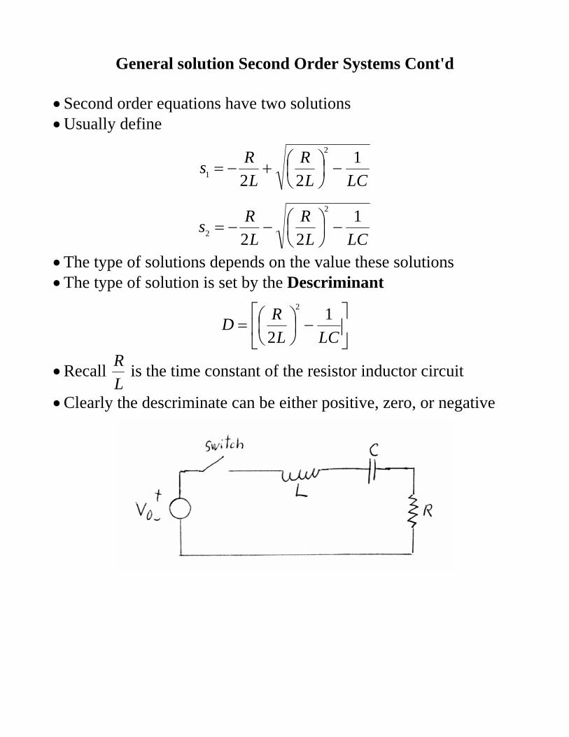
General solution Second Order Systems Cont'd • Second order equations have two solutions • Usually define

LCLR

LRs 1

22

2

1 −⎟⎠⎞

⎜⎝⎛+−=

LCLR

LRs 1

22

2

2 −⎟⎠⎞

⎜⎝⎛−−=

• The type of solutions depends on the value these solutions • The type of solution is set by the Descriminant

⎥⎦

⎤⎢⎣

⎡−⎟

⎠⎞

⎜⎝⎛=

LCLRD 1

2

2

• Recall LR is the time constant of the resistor inductor circuit

• Clearly the descriminate can be either positive, zero, or negative

3 solutions of the Second Order Systems • What the Descriminant represents is about energy flows

⎥⎦

⎤⎢⎣

⎡−⎟

⎠⎞

⎜⎝⎛=

LCLRD 1

2

2

• How fast is energy transferred from the L to the C • How fast is energy lost to the resistor • There are three cases set by the descriminant • D > 0 : roots real and unequal • In electronics called the overdamped case • D = 0 : roots real and equal • In electronics the critically damped case • D < 0 : roots complex and unequal • In electronics: the underdamped case: very important

Second Order Solutions • Second order equations are all about the energy flow • Consider the spring case • The spring and the mass have energy storage • The damping pot losses the energy • The critical factor is how fast is energy lost • In Overdamped the energy is lost very fast • The block just moves to the rest point • Critically Damped the loss rate is smaller • Just enough for one movement up and down • For Underdamped spring moves up and down • Energy is transferred from the mass to the spring and back again • Loss rate is smaller than the time for transfer

Complex Numbers • Imaginary numbers necessary for second order solutions • Imaginary number j

1−=j

• Note: in math imaginary number is called i • But i means current in electronics so we use j • Complex numbers involve Real and Imaginary parts

WW jIRW +=r

• May designate this in a vector coordinate form:

( )WW IRW ,=r

• Example:

( ) 2)Im(1Re)2,1(21

===+=

WWjW

r

Complex Numbers Plotted • In electronics plot on X-Y axis • X axis real, Y axis is imaginary • A vector represents the imaginary number has length • Vector has a magnitude M • Vector is at some angle θ to (theta) the real axis • Then the real and imaginary parts are

( ) ( )θcosRe MRWal W ==

( ) ( )θsinIm MIWaginary W ==

( ) ( )[ ]θθ sincos jMW +=r

• The magnitude

( ) ( )22

WWIRWWMag +==

rr

• The angle

⎟⎟⎠

⎞⎜⎜⎝

⎛=

W

W

RIarctanθ

Thus can give the vector in polar coordinates

( ) θθ ∠== MMW ,r

Complex Numbers and Exponentials • Polar coordinates are connected to complex numbers in exp • Consider an exponential of a complex number

( ) ww jIRMW +== θ,r

• This is given by the Euler relationship

( ) ( ) ( )[ ]θθθ sincosexp jj +=

( ) ( ) ( )[ ]θθθ sincosexp jMjMW +==r

• This relationship is very important for electronics • Used in second order circuits all the time.

Overdamped RLC • This is a very common case • In RLC series circuits this is the large resistor • Energy loss in the resistor much greater than energy transfers • Two real roots to the characteristic equation

LCLR

LRs 1

22

2

−⎟⎠⎞

⎜⎝⎛±−=

• The solution is a double exponential decay

( ) ( ) ( )tsAtsAti 2211 expexp +=

• As R is increased damping increases • Get the overdamped case

Overdamped RLC Energy Flows • For the example case L = 5 mH, C = 2 µF, R = 200 Ω • Also assume C is charged to 10 V at t = 0 • Initially energy starts in the Capacitor C • Some energy transfers to the Inductor L • C looses charge much faster than L gains current • So energy starts to rise in L but only to a limited level • Then energy is removed from both by the resistor

Overdamped RLC Initial Conditions • For the overdamped case the s’s are real & different

( ) ( ) ( )tsAtsAti 2211 expexp +=

• To solve the constants A need the initial conditions • For second order need two conditions • Thus both initial current & its derivative • This varies from circuit to circuit • In the case of a charged C switched into the circuit • Since L acts as an open initially then i(0) = 0, thus

( ) 210 AAi += • Thus

12 AA −=

• Again since the inductor acts open at time zero & i(0)=0 • Thus voltage drop across the resistor is zero

( ) ( ) ( )dt

diLVV LC

000 ==

( ) ( )L

Vdt

di c 00=

Overdamped RLC Full Solution • Now using substituting A equation into the exp equation

( ) ( ) ( )tsAtsAti 2111 expexp −=

• To solve the constants A with the derivative initial condition

( ) ( ) ( )[ ]tsstssAdt

tdi22111 expexp −=

• Now applying the initial condition derivative

( ) ( ) ( )[ ] [ ] ( )L

VssAssAdttdi c 00exp0exp0

211211 =−=−==

• Now solving the equations

( )[ ]Lss

VA C

211

0−

=

( ) ( )[ ] ( ) ( )[ ]tsts

LssVti C

2121

expexp0−

−=

Overdamped RLC Circuit Example • For the example case L = 5 mH, C = 2 µF, R = 200 Ω • Solving for the roots first what are the discriminate values

sec501sec102005.02

2002

14 µττ

==×=×

=⎟⎠⎞

⎜⎝⎛ −

LR

( )28

6 sec10102005.0

11 −

−=

××=

LC

( )[ ] 288242

sec1031010212

−×=−×=⎥⎦

⎤⎢⎣

⎡−⎟

⎠⎞

⎜⎝⎛=

LCLRD

• Thus gives

1382

1 sec1068.2103005.02

200122

−×−=×+×

−=−⎟⎠⎞

⎜⎝⎛+−=

LCLR

LRs

1482

2 sec1073.3103005.02

200122

−×−=×−×

−=−⎟⎠⎞

⎜⎝⎛−−=

LCLR

LRs

• Thus ( )

[ ] [ ] ALss

VA C 244

211 1077.5

005.01087.51087.1100 −×=

×+×=

−=

( ) ( ) ( )[ ]Ati 42 1073.3exp10368.2exp1077.5 ×−−×−×= −

Critical Damped RLC • If we decrease the damping (resistance) energy loss decreases • Change the exponential decay until discriminant=0

012

2

=⎥⎥⎦

⎤

⎢⎢⎣

⎡−⎟

⎠⎞

⎜⎝⎛=

LCLRD

LCLR 1

2

2

=⎟⎠⎞

⎜⎝⎛

• This is the point called critical damping • Difficult to achieve: only small change in R moves from this point • Small temperature change will cause that to occur • Energy transfer from C to L is now smaller than loss in R

Critical Damped RLC Solutions • The characteristic equation has two identical solutions

0LC1s

LRs2 =++

LRss

221 −==

• This is a special case, with special solution

( ) [ ] ⎟⎠⎞

⎜⎝⎛−+=

LRttAAti2

exp21

Why this solution? Given in the study differential equations in math

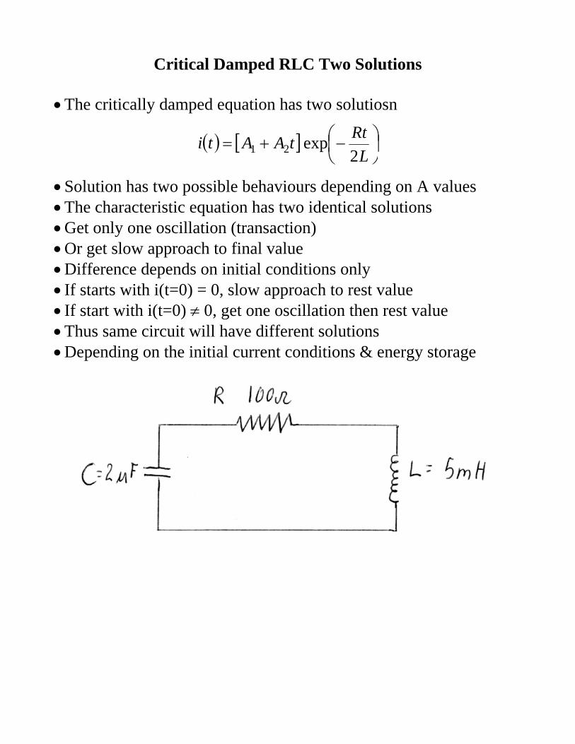
Critical Damped RLC Two Solutions • The critically damped equation has two solutiosn

( ) [ ] ⎟⎠⎞

⎜⎝⎛−+=

LRttAAti2

exp21

• Solution has two possible behaviours depending on A values • The characteristic equation has two identical solutions • Get only one oscillation (transaction) • Or get slow approach to final value • Difference depends on initial conditions only • If starts with i(t=0) = 0, slow approach to rest value • If start with i(t=0) ≠ 0, get one oscillation then rest value • Thus same circuit will have different solutions • Depending on the initial current conditions & energy storage

Critical Damped RLC Example i(0)=0 • Keeping L & C the same • If R is increased 100 ohm get critical damping • Here L = 5 mH, C = 2 µF, R = 100 Ω • Also assume C is charged to 10 V at t = 0 • Also assume C is charged to 10 V at t = 0 but i(t)=0 • This is the no oscillation case

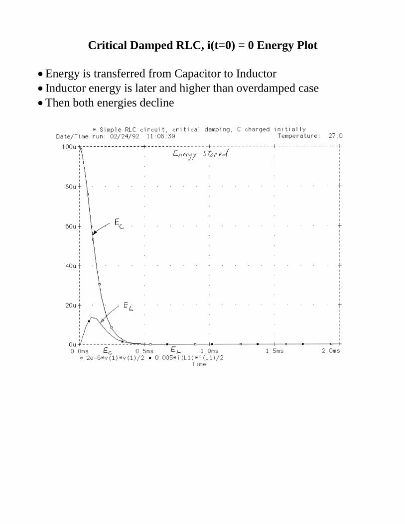
Critical Damped RLC, i(t=0) = 0 Energy Plot • Energy is transferred from Capacitor to Inductor • Inductor energy is later and higher than overdamped case • Then both energies decline

Critical Damped RLC i(0)=0 Solution • We define the Damping Decay Constant α

14 sec10005.02

1002

−=×

==L

Rα

• The damping constant gives how fast energy is decaying • The basic Critical Damping equation is

( ) [ ] ⎟⎠⎞

⎜⎝⎛−+=

LRttAAti2

exp21

• Solving for A constants from the initial conditions • Since current is at t=0 is zero then

( ) [ ] 121 20exp000 AL

RAAti =⎟⎠⎞

⎜⎝⎛−+===

( ) ⎟⎠⎞

⎜⎝⎛−=

LRttAti2

exp2

• Again since the inductor acts open at time zero

( ) ( )L

Vdt

di c 00=

• Now applying this to the equation

( )222 2

012

0exp2

12

exp0 AL

RL

RAL

RtL

RtAdttdi

=⎥⎦⎤

⎢⎣⎡ −⎟⎠⎞

⎜⎝⎛−=⎥⎦

⎤⎢⎣⎡ −⎟⎠⎞

⎜⎝⎛−=

=

• Thus at time t=0 then ( ) AL

VA c 2000005.0100

2 ===

( ) [ ] ( ) At10expt2000L2

RtexptAti 42 −=⎟

⎠⎞

⎜⎝⎛−=

Critical Damped RLC, i(t=0) = 0 Voltage Plot • Capacitor voltage starts at 10 V and declines • Inductor voltage starts at 10 V then reverses & declines • Resistor voltage starts at zero, rises to peak above Vc then declines

Critical Damped RLC, i(t=0) = 0 Current Plot • Current rises to peak due to A2t term • Then current declines near exponential with α

( ) [ ] ( ) At10expt2000L2

RtexptAti 42 −=⎟

⎠⎞

⎜⎝⎛−=

Critical Damped RLC, i(t=0) ≠ 0 • Now consider the case when i(t=0) is non zero • The practical case is when capacitor is uncharged • But inductor has current flowing in it • The equation has both constants nonzero

( ) [ ] ⎟⎠⎞

⎜⎝⎛−+=

LRttAAti2

exp21

• Again the example have L = 5 mH, C = 2 µF, R = 100 Ω • Now assume L initially carries 100 mA at t = 0, thus

( ) mA100AI0ti 10 ====

• Since C acts as a short at time t=0 thus VC(t=0) = 0 • Then the only voltage drop is across the resistance

( ) 000 =

=+

dttdiLRI

( )LRI

dttdi 00

−==

Critical Damped RLC, i(t=0) ≠ 0 Equation • Now for the derivative of the equation

( ) [ ] ⎟⎠⎞

⎜⎝⎛−

⎭⎬⎫

⎩⎨⎧

⎟⎠⎞

⎜⎝⎛−++=

LRt

LRtAAA

dttdi

2exp

2212

• For the initial conditions

( ) [ ]L

RIAL

RAAL

RL

RAAdttdi

2220exp

20 0

21212 −=⎟⎠⎞

⎜⎝⎛−=⎟

⎠⎞

⎜⎝⎛−

⎭⎬⎫

⎩⎨⎧

⎟⎠⎞

⎜⎝⎛−+=

=

• Relating this to the resistance

( )LRI

LRIA

dttdi 00

2 20

−=−==

AL

RIA 1000005.02

1.01002

02 −=

××

−==

• Thus the critically damped i(t=0)≠0 current equation is

( ) [ ] [ ] ( ) At10expt10001.0L2

RtexptAAti 421 −−=⎟

⎠⎞

⎜⎝⎛−+=

• Thus the current will reverse direction at t=0.1 msec.

Critical Damped RLC, i(t=0) ≠ 0 Current Plot • Current reaches zero at t=0.1 msec • Reverses, reaches peak at t=0.2 msec then declines

( ) [ ] [ ] ( ) At10expt10001.0L2

RtexptAAti 421 −−=⎟

⎠⎞

⎜⎝⎛−+=

Critical Damped RLC, i(t=0) ≠ 0 Energy Plot • Inductor energy falls to minimum at t=0.1 msec • Energy is transferred from L to C and back to L

Critical Damped RLC, i(t=0) ≠ 0 Energy Plot Expanded • Capacitor energy reaches max when EL is minimum • Then Inductor energy rises again • Both energies decay

Critical Damped RLC, i(t=0) ≠ 0 Voltage Plot • Inductor voltage starts at 10 V and declines • Resistor voltage starts at -10 V and rises to zero

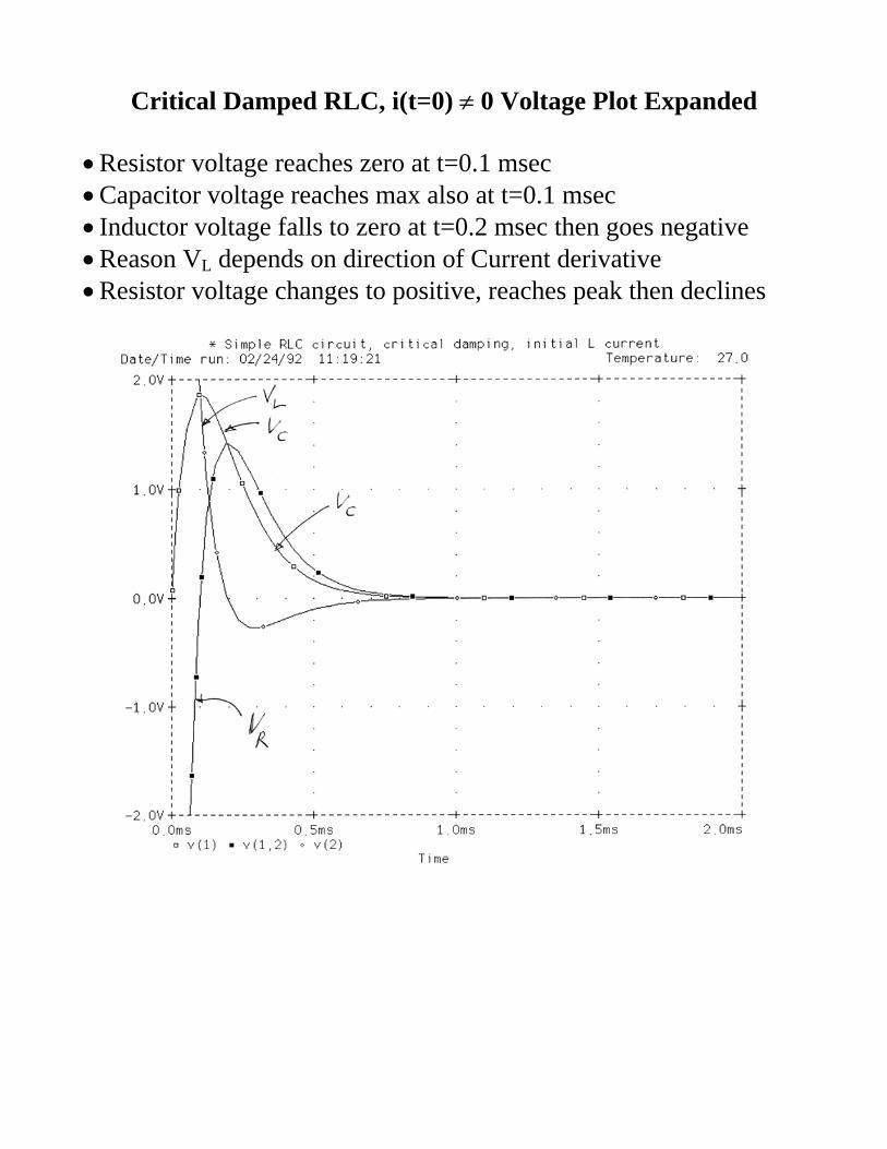
Critical Damped RLC, i(t=0) ≠ 0 Voltage Plot Expanded • Resistor voltage reaches zero at t=0.1 msec • Capacitor voltage reaches max also at t=0.1 msec • Inductor voltage falls to zero at t=0.2 msec then goes negative • Reason VL depends on direction of Current derivative • Resistor voltage changes to positive, reaches peak then declines