Performance Evaluation 65 (2008) 366–381www.elsevier.com/locate/peva

A conditional probability approach to M /G/1-like queues

Alexandre Brandwajna,∗, Hongyun Wangb

a Department of Computer Engineering, Baskin School of Engineering, University of California, Santa Cruz, CA 95064, USAb Department of Applied Mathematics & Statistics, Baskin School of Engineering, University of California, Santa Cruz, CA 95064, USA

Received 29 August 2006; received in revised form 5 May 2007; accepted 20 September 2007Available online 5 October 2007

Abstract

Following up on a recently renewed interest in computational methods for M /G/1-type processes, this paper considers anM /G/1-like system in which the service time distribution is represented by a Coxian series of memoryless stages. We present a novelapproach to the solution of such systems. Our method is based on conditional probabilities, and provides a simple, computationallyefficient and stable approach to the evaluation of the steady-state queue length distribution. We provide a proof of the numerical sta-bility of our method. Without explicit use of matrix-geometric techniques or stochastic complementation, we are able to handle sys-tems with state-dependent service and arrival rates. The proposed approach can be used to compute the queue length distribution forboth finite and infinite M /G/1-like queues. In the case of an infinite, state-independent queue, our method allows us to show usingelementary tools that the queue length distribution is asymptotically geometric. The parameter of the asymptotic geometric can beexpressed through a simple set of equations, easily solved using fixed point iteration. Our approach is very thrifty in terms of mem-ory requirements, easy to implement, and generally fast. Numerical examples illustrate the performance of the proposed method.c© 2007 Elsevier B.V. All rights reserved.

Keywords: M /G/1-like queues; Coxian distribution; State-dependent service; Conditional probability; Queue length distribution; Recurrentsolution; Numerical stability; Computational efficiency; Asymptotic geometric distribution; Algorithms; Performance

1. Introduction

M /G/1-type queues are an essential tool in the performance analysis of computers and computer networks. Devicesranging from volumes in a storage subsystem to stations in an optical ring network have been represented as M /G/1queues. Oftentimes, it is necessary to take into account the finite buffer space at such devices (e.g. to properly sizethe buffers), and, in some systems, the fact that the service rate may depend on the number of customers in thesystem (e.g. due to contention for shared resources). The efficient and numerically stable solution of such queues, inparticular, the calculation of the stationary queue length probabilities, is therefore of importance. Recently, there hasbeen a renewed interest in computational methods for M /G/1-type processes [27,30]. As discussed by Stathopouloset al. [30], matrix analytic techniques introduced by Neuts [23,24] are often used to evaluate such processes. Inparticular, Ramaswami’s algorithm [25,21] provides a numerically stable approach to the computation of steady-stateprobabilities in an M /G/1-type system. This algorithm is based on stochastic complementation [28], and its fastestimplementation uses the FFT [22] (cf. [30]). The ETAQA method [27] has been proposed as an alternative for the

∗ Corresponding author. Tel.: +1 831 459 4023.E-mail addresses: alexb@soe.ucsc.edu (A. Brandwajn), hongwang@ams.ucsc.edu (H. Wang).

0166-5316/$ - see front matter c© 2007 Elsevier B.V. All rights reserved.doi:10.1016/j.peva.2007.09.002

A. Brandwajn, H. Wang / Performance Evaluation 65 (2008) 366–381 367

computation of the moments of the queue length distribution (but not the distribution itself). Stathopoulos et al. [30]derive a new formulation for ETAQA and demonstrate its links with the Ramaswami’s method.

The large body of previous work includes the work by Gaver et al. [14], who consider finite queues in randomlychanging environments, and derive a numerical method involving recursive determination of certain matrices. Brightand Taylor [10] extend the logarithmic reduction algorithm proposed by Latouche and Ramaswami [18] to level-dependent infinite queues. They note possible numerical problems when recursively calculating matrices involved inthe solution. Such problems are also mentioned in Gaver et al. [14]. Latouche shows in [17] that Newton’s methodapplied to non-linear equations in Markov chains is quadratically convergent although not very attractive because ofits computational complexity. Bini and Meini [6] extend the cyclic reduction techniques to infinite block matrices, andlater propose an improvement based on FFT to lower computational cost and increase numerical stability [7]. Akarand Sohraby [1] propose an invariant subspace approach with at least quadratic convergence rates and potentiallyimproved accuracy due to the avoidance of truncation. Ramaswami and Taylor [26] study the generalization ofmatrix-geometric stationary distribution to level-dependent quasi-birth-and-death processes. More recently, Beanet al. [3] consider quasistationary distributions for level-dependent processes and their computation using methodsakin to the Latouche–Ramaswami algorithm. Ye [31] studies the theoretical properties of the Latouche–Ramaswamilogarithmic reduction algorithm, pointing out numerical stability issues and offering an alternative based on a morestable algorithm for inverting a diagonally dominant matrix.

The asymptotic behavior of an infinite queue has been studied, among others, by Bean et al. [4] who considerquasi-birth-and-death processes with decomposable spaces, and use the matrix-geometric form of the steady stateprobability vector to derive a numeric method for computing the “caudal characteristic factor” of the process usingmatrices smaller than earlier traditional methods. Knessl et al. [15] consider a state-dependent M /G/1 where theinterarrival and the service time distributions depend on the amount of unfinished work in the system. They applyperturbation methods to derive approximations for several measures pertaining to the unfinished work and the meanbusy period in such a queue. In a related work, Knessl et al. [16] study a GI/G/1 queue with a similar form of statedependence using the same perturbation methods.

The reader is referred to the books by Latouche and Ramaswami [19], and by Bini et al. [5] for an overview ofproperties of matrix analytic approaches and numerical methods for quasi-birth-and-death problems and M /G/1-typeMarkov chains. Practical considerations and software implementation for several of the methods mentioned above arediscussed by Bini et al. [8,9].

In this paper, we consider an M /G/1-like system in which the service time distribution is represented by aCoxian [12] series of memoryless stages. It is well known that a Coxian distribution can approximate arbitrarilyclosely any distribution, and a two-stage Coxian can be used to match the first two moments of any distribution [2]whose coefficient of variation is greater than 1. Several authors have considered algorithms for matching an arbitrarydistribution by a Coxian, e.g. [11,29,13,20].

Our method is based on conditional probabilities, and provides a simple, computationally efficient and numericallystable approach to the evaluation of the steady-state queue length distribution. Without any explicit use of matrix-geometric techniques or stochastic complementation, we are able to solve systems with state-dependent service andarrival rates. As a result, the proposed approach can be used for finite M /G/1-like queues as well. In the case of aninfinite, state-independent queue, the form of the queue length distribution indicates that it is asymptotically geometricwith a coefficient given as a solution of a simple set of equations, easily solved via fixed point iteration. To the best ofour knowledge, the proposed method is novel.

This paper is organized as follows. In Section 2 we describe in more detail the queue considered and presentour computational approach. Section 3 is devoted specifically to the case of an infinite state-independent queue andits asymptotically geometric queue length distribution. In Section 4 we outline the proof of numerical stability ofour method. Section 5 presents numerical results to illustrate the behavior of our method, and Section 6 concludesthis paper. Additionally, in the Appendix we show that the conditional probability on which we base our approachconverges to a single fixed point in the case of an infinite state-independent queue.

2. M/G/1-like model and its recurrent solution

2.1. Model considered and its equations

The single-server queuing model considered is shown in Fig. 1.

368 A. Brandwajn, H. Wang / Performance Evaluation 65 (2008) 366–381

Fig. 1. M /G/1-type queue with Coxian-like service.

We assume that customers arrive from a quasi-Poisson source with rate λ(n) where n denotes the current number ofcustomers in the system. The service of a customer is represented by a state-dependent Coxian-like distribution [12]with a total of k stages. Both the completion rates of the memoryless stages and the exit probabilities in this distributionmay depend on the number of customers in the queue. We denote by µi (n) the service rate of stage i and by qi (n) theprobability that the customer completes its service following stage i, i = 1, . . . , k. We let qi (n) = 1 − qi (n) denotethe probability that the customer proceeds to stage i + 1 upon completion of stage i when there are n customersin the system. We assume that µi (n) > 0, i = 1, . . . , k, 0 < qi (n) ≤ 1 for i < k and qk(n) = 0. Note that ourformulation allows not only the mean value but also the nature of the service time distribution to change as the numberof customers in the queue changes.

We consider the system of Fig. 1 in steady state, and we use the couple (n, i) where n (n ≥ 1) is the currentnumber of customers and i (i = 1, . . . , k) is the current stage of service to describe the state of the system when it isnot idle. We denote by p(n, i) the corresponding steady state probability, and by p(0) the probability that there are nocustomers in the system.

It is straightforward to obtain the balance equations for the corresponding state probabilities

p(1, 1)[λ(n) + µ1(n)] =

k∑i=1

p(n + 1, i)µi (n + 1)qi (n + 1) + p(0)λ(0) (1)

p(1, i)[λ(n) + µi (n)] = p(n, i − 1)µi−1(n)qi−1(n), i > 1 (2)

for n = 1, and

p(n, 1)[λ(n) + µ1(n)] =

k∑i=1

p(n + 1, i)µi (n + 1)qi (n + 1) + p(n − 1, 1)λ(n − 1) (3)

p(n, i)[λ(n) + µi (n)] = p(n, i − 1)µi−1(n)qi−1(n) + p(n − 1, i)λ(n − 1), i > 1 (4)

for n > 1.These balance equations can be transformed into equations for the conditional probabilities of the service stage

number given the current number of customers, and solved as a simple recurrence.

2.2. Recurrent solution

Our goal is to transform the standard balance equations (1)–(4) into easy-to-evaluate recurrence relations. Wedenote by p(i | n) the conditional probability that the current service stage is i given that the number of customers isn, and by p(n) the marginal probability that the number of customers in our M /G/1-like queue is equal to n. For alln ≥ 1 and i = 1, . . . , k we have

p(n, i) = p(i | n)p(n). (5)

From (5) and the balance equations (1)–(4), it is easy to see that p(n) can be expressed as

p(n) =1G

n∏l=1

λ(l − 1)/u(l), (6)

where G is a normalizing constant and

u(n) =

k∑i=1

p(i | n)µi (n)qi (n) (7)

A. Brandwajn, H. Wang / Performance Evaluation 65 (2008) 366–381 369

u(n) is the conditional rate of completion given n, and 1/u(n) can be viewed as the mean service time given that thereare n customers in the system.

Substituting (5) and (6) into the balance equations, and using the fact that p(n) > 0 for all feasible values of n, wereadily obtain the equations for the conditional probabilities p(i | n)

p(1 | 1)[λ(1) + µ1(1)] = λ(1) + u(1) (8)

p(i | 1)[λ(1) + µi (1)] = p(i − 1 | 1)µi−1(1)qi−1(1), i > 1 (9)

for n = 1, and

p(1 | n)[λ(n) + µ1(n)] = λ(n) + p(1 | n − 1)u(n) (10)

p(i | n)[λ(n) + µi (n)] = p(i − 1 | n)µi−1(n)qi−1(n) + p(i | n − 1)u(n), i > 1 (11)

for n > 1.Since we must have

k∑i=1

p(i | n) = 1 for n ≥ 1, (12)

we can express the solution of (8) and (9) as

p(i | n = 1) =1H

i∏j=2

µ j−1(1)q j−1(1)/[λ(1) + µ j (1)], (13)

where H is a normalizing constant. The empty product is equal to 1 by convention, so that we have p(1 | 1) = 1/H .Note that Eqs. (8) and (9), together with the normalizing condition (12), imply that we must have u(1) < µ1(1) in thesteady state of our system.

We now consider Eqs. (10) and (11) for increasing values of n = 2, 3, . . . For each n, the p(i | n − 1) areknown from the preceding step, so that (10) and (11) is a system of k equations for the k conditional probabilitiesp(i | n), i = 1, . . . , k. We note that Eqs. (10) and (11) involve u(n), a linear combination of the conditionalprobabilities p(i | n), and we can express the latter as

p(i | n) = bi (n)λ(n) + ci (n)u(n). (14)

From (10) we have

b1(n) = 1/[λ(n) + µ1(n)], and c1(n) = p(1 | n − 1)/[λ(n) + µ1(n)]. (15)

Eq. (11) yields the following recurrence

bi (n) = bi−1(n)µi−1(n)qi−1(n)/[λ(n) + µi (n)],

ci (n) = [ci−1(n)µi−1(n)qi−1(n) + p(i | n − 1)]/[λ(n) + µi (n)] for i > 1.(16)

Having computed the coefficients bi (n) and ci (n) from the above recurrence, we determine u(n) from the normalizingcondition (12)

u(n) =

[1 − λ(n)

k∑i=1

bi (n)

]/ k∑i=1

ci (n). (17)

For n = 1, we can use a similar approach or the solution form given by (13). Note that the recurrence itself (15) and(16) involves no subtractions to detract from numerical stability. A formal proof of stability is outlined in Section 4.Space requirements of our recurrent computation are very modest since we need only one set (for a single value ofn) of the conditional probabilities p(i | n) at any time. Even the values of u(n) need not be kept if we embed ourrecurrence into the computation of the marginal probability p(n). The latter is given by the familiar product-formformula (6) identical to that of a state-dependent M /M /1 queue with arrival rate λ(n) and service rate u(n). Clearly,if λ(n) vanishes for some value of n, the customer population is limited and the recurrence has a “natural” stopping

370 A. Brandwajn, H. Wang / Performance Evaluation 65 (2008) 366–381

point. If the population in the queue is unrestricted, as would be the case with a Poisson source, the computation willhave to stop when values of p(i | n) (and thus u(n)) for consecutive values of n no longer change more than somereasonable tolerance we fix as the convergence criterion. To the best of our knowledge, the proposed approach to thecomputation of the stationary queue length probabilities in an M /G/1-like queue is novel. The next section is devotedto the particular case of an infinite state-independent queue.

3. Infinite state-independent queue

We now restrict our attention to the particular case of an M /G/1-like queue with Poisson arrivals and standardCoxian service distribution. Specifically, we have λ(n) = λ, µi (n) = µi , and qi (n) = qi . Since the approachpresented in the preceding section involves a recurrent computation of the conditional probabilities p(i | n)

for consecutive values of n, it might seem that, for the open queue, the method would require the solution ofan infinite number of such recurrences. In this section we argue that, in practice, these conditional probabilitiestend to quickly reach a limiting value, so that only a relatively small number of recurrences need to be solved.In the process, we demonstrate the asymptotically geometric form of the steady-state distribution p(n) for largen.

For the queue considered, the equations for the conditional probability for n = 1 become

p(1 | n = 1)[λ + µ1] = λ + u(1) (18)

p(i | n = 1)[λ + µi ] = p(i − 1 | n = 1)µi−1qi−1, i > 1, (19)

and for n > 1 we have

p(1 | n)[λ + µ1] = λ + p(1 | n − 1)u(n) (20)

p(i | n)[λ + µi ] = p(i − 1 | n)µi−1qi−1 + p(i | n − 1)u(n), i > 1. (21)

As n tends to infinity, the conditional probability p(i | n) and u(n) tend to their limiting values which we denote byp(i) and u, respectively. A rigorous proof of this convergence is presented in the Appendix. Given the form of p(n)

in (6), the convergence to limiting values means that we have asymptotically for large n,

p(n + 1)/p(n) ≈ λ/u, (22)

i.e., the steady-state distribution is asymptotically geometric.In our numerical experiments, we found that, typically, the solution of Eqs. (20) and (21) tends rapidly to the

limiting distribution p(i) as n increases. Consequently, we can use the following computational approach to obtainthe queue length distribution for the infinite state-independent queue. Select a convergence criterion, e.g. ‖p(i | n)

− p(i | n −1)‖ < ε with some reasonable value of ε, and let n be the value of n for which the convergence is attained.We can express the steady-state distribution p(n) as

p(n) ≈1G

n∏l=1

λ/u(l), n ≤ n[n∏

l=1

λ/u(l)

](λ/u)n−n, n > n.

(23)

The normalizing constant G can be written as

G = 1 +

n−1∑n=1

n∏l=1

λ/u(l) +

[n∏

l=1

λ/u(l)

]1

1 − (λ/u).

Thus, we use the recurrence described in Section 2.2 (13)–(17) for n = 1, . . . , n (i.e. simply until convergence hasbeen reached in the computation of p(i | n) and u(n)). Once convergence has been attained, we use the last computedvalue for u(n) as the limiting value u in the geometric tail of the distribution p(n). With this approach, the expected

A. Brandwajn, H. Wang / Performance Evaluation 65 (2008) 366–381 371

number of customers in the system can be written as

n ≈1G

{n∑

n=1

np(n) +

[n

1 − (λ/u)+

(λ/u)

[1 − (λ/u)]2

] n∏l=1

λ/u(l)

}.

Clearly, the system is stable as long as λ < u.In practice, it has been our experience that convergence to u tends occur quite rapidly, resulting typically in

moderate values for n. In Section 5, we present numerical results to illustrate the behavior of our method.Our recurrent algorithms produce the set of u(n) for n = 1, . . . , n, i.e., until convergence to u. If desired, the

limiting value u can also be computed independently as follows. The limiting conditional probabilities p(i) and thelimiting service rate value u satisfy the following equations

p(1)[λ + µ1] = λ + p(1)u (24)

p(i)[λ + µi ] = p(i − 1)µi−1qi−1 + p(i)u, i > 1. (25)

Eqs. (24) and (25) can be easily (and, generally, rapidly) solved using a fixed-point iteration. Starting with an initialprobability distribution p0(i) (we use a superscript to denote the iteration number) and the corresponding value u0,we compute values at iteration j

p j (1) ∝ [λ + p j−1(1)u j−1]/[λ + µ1] (26)

p j (i) ∝ [ p j (i − 1)µi−1qi−1 + p j−1(i)u j−1]/[λ + µi ], i > 1. (27)

At each iteration we normalize the values so as to have∑k

i=1 p j (i) = 1. This allows us to determine the limitingvalues p(i) and u. The latter is the service rate value for the asymptotically geometric state probability. We do nothave a formal proof of convergence of this iterative scheme. In practice, it has converged without any damping in theiteration for all the cases investigated.

The next section is devoted to a formal proof that our recurrent algorithm is numerically stable.

4. Stability of recurrent solution

Our goal in this section is to show that our recurrent solution described in Section 2 is computationally stable. Forour purposes here, we find it convenient to rewrite the recurrence as

p(i | n)[λ(n) + µi (n)] = p(i − 1 | n)µi−1(n)qi−1(n) + λ(n)δi,1 + p(i | n − 1)u(n), (28)

where we use the following notation

p(i | 0) =

{1, i = 10, i > 1,

p(0 | n) = 0 and δi,1 =

{1, i = 10, i 6= 1.

As described in Section 2, the solution can be expressed as

p(i | n) = bi (n)λ(n) + ci (n)u(n) (29)

with the coefficients bi (n) and ci (n) given by

bi (n)[λ(n) + µi (n)] = bi−1(n)µi−1(n)qi−1(n) + δi,1 (30)

ci (n)[λ(n) + µi (n)] = ci−1(n)µi−1(n)qi−1(n) + p(i | n − 1). (31)

By convention, we let b0(n) = c0(n) = 0. u(n) is given by (17), i.e.

u(n) =

[1 − λ(n)

k∑i=1

bi (n)

]/ k∑i=1

ci (n).

We assume that the Coxian service time distribution has indeed k stages, so that

µi (n) > 0, i = 1, . . . , k, 0 < qi (n) ≤ 1 for i < k and qk(n) = 0.

We start by showing that our recurrence for p(i | n) produces positive values.

372 A. Brandwajn, H. Wang / Performance Evaluation 65 (2008) 366–381

Lemma 1. If p(1 | n − 1) > 0 and p(i | n − 1) ≥ 0 for i > 1, then we have

(1) bi (n) > 0 and ci (n) > 0 for i ≥ 1,(2) u(n) > 0, and(3) p(i | n) > 0 for i ≥ 1.

Proof. (1) Follows directly from (30) and (31).(2) Summing (30) over all values of i and using the fact that qk(n) = 0, we have

k∑j=1

b j (n)[λ(n) + µ j (n)] =

k∑j=1

b j (n)µ j (n)q j (n) + 1.

Rearranging the terms and using the fact that q j (n) = 1 − q j (n), we get

1 − λ(n)

k∑j=1

b j (n) =

k∑j=1

b j (n)µ j (n)q j (n) > 0, and hence u(n) > 0.

(3) Follows directly from the results of (1) and (2).

Lemma 1 tells us that p(i | n) > 0 for i ≥ 1 and n ≥ 1. �

We now consider a set of perturbed conditional probabilities (the perturbation corresponding to floating pointround-off errors)

p(i | n − 1) = p(i | n − 1) + ∆p(n−1)i .

Since the conditional probability is normalized at each step of the recurrence, the perturbations ∆p(n−1)i must

satisfy∑k

i=1 ∆p(n−1)i = 0. We also assume that the perturbations are small so that we have p(i | n − 1) > 0. (30)

shows that the perturbation does not affect bi (n). Let ci (n) = ci (n)+∆c(n−1)i be the solution of (31) when p(i | n−1)

is replaced by p(i | n − 1). ∆p(n−1)i and ∆c(n)

i are related by

∆c(n)i [λ(n) + µi (n)] = ∆c(n)

i−1µi−1(n)qi−1(n) + ∆p(n−1)i . (32)

In Lemma 2 we bound relative perturbations in pi (n − 1) in terms of relative perturbations in ci (n).

Lemma 2. ∆p(n−1)i and ∆c(n)

i satisfy

maxj

∆c(n)j

c j (n)≤ max

j

∆p(n−1)j

p( j | n − 1)

minj

∆c(n)j

c j (n)≥ min

j

∆p(n−1)j

p( j | n − 1).

Proof. See Appendix. �

Let p(i | n) = p(i | n) + ∆p(n)i be the conditional probabilities at n corresponding to p(i | n − 1). p(i | n) is

expressed in (29) as

p(i | n) = bi (n)λ(n) + ci (n)u(n),

where

u(n) =

[1 − λ(n)

k∑i=1

bi (n)

]/ k∑i=1

ci (n).

The next lemma relates ∆p(n)i to ∆c(n)

i .

A. Brandwajn, H. Wang / Performance Evaluation 65 (2008) 366–381 373

Lemma 3. ∆p(n)i satisfies

∆p(n)i

u(n)ci (n)=

1

1 + ∆β(n)

[∆c(n)

i

ci (n)− ∆β(n)

],

where

∆β(n)=

k∑j=1

∆c(n)j

/ k∑j=1

c j (n).

Proof. See Appendix. �

We now have the elements to prove the stability of our recurrent algorithm. Consider a function “measuring” themagnitude of the relative error in p(i | n)

g(n) =

maxj

∆p(n)j

p( j |n)− min

j

∆p(n)j

p( j |n)

1 + minj

∆p(n)j

p( j |n)

.

Theorem 1. g(n) satisfies

(1) g(n) ≤ g(n − 1)

(2) max j |∆p(n)

jp( j |n)

| ≤ g(n).

Proof. (1)∑k

j=1 ∆p(n)j = 0 implies

maxj

∆p(n)j

p( j | n)≥ 0 and min

j

∆p(n)j

p( j | n)≤ 0. (33)

Using (29) and the results of Lemma 1, we have

maxj

∆p(n)j

p( j | n)≤ max

j

∆p(n)j

u(n)ci (n)and min

j

∆p(n)j

p( j | n)≥ min

j

∆p(n)j

u(n)ci (n).

Substituting into function g(n) yields

g(n) ≤

maxj

∆p(n)j

u(n)c j (n)− min

j

∆p(n)j

u(n)c j (n)

1 + minj

∆p(n)j

u(n)c j (n)

.

From the results of Lemmas 2 and 3 it follows[max

j

∆p(n)j

u(n)c j (n)− min

j

∆p(n)j

u(n)c j (n)

]=

1

1 + ∆β(n)

[max

j

∆c(n)j

c j (n)− min

j

∆c(n)j

c j (n)

]

≤1

1 + ∆β(n)

[max

j

∆p(n−1)j

p( j | n − 1)− min

j

∆p(n−1)j

p( j | n − 1)

]and

1 + minj

∆p(n)j

u(n)c j (n)=

1

1 + ∆β(n)

[1 + min

j

∆c(n)j

c j (n)

]

≥1

1 + ∆β(n)

[1 + min

j

∆p(n−1)j

p( j | n − 1)

]> 0.

374 A. Brandwajn, H. Wang / Performance Evaluation 65 (2008) 366–381

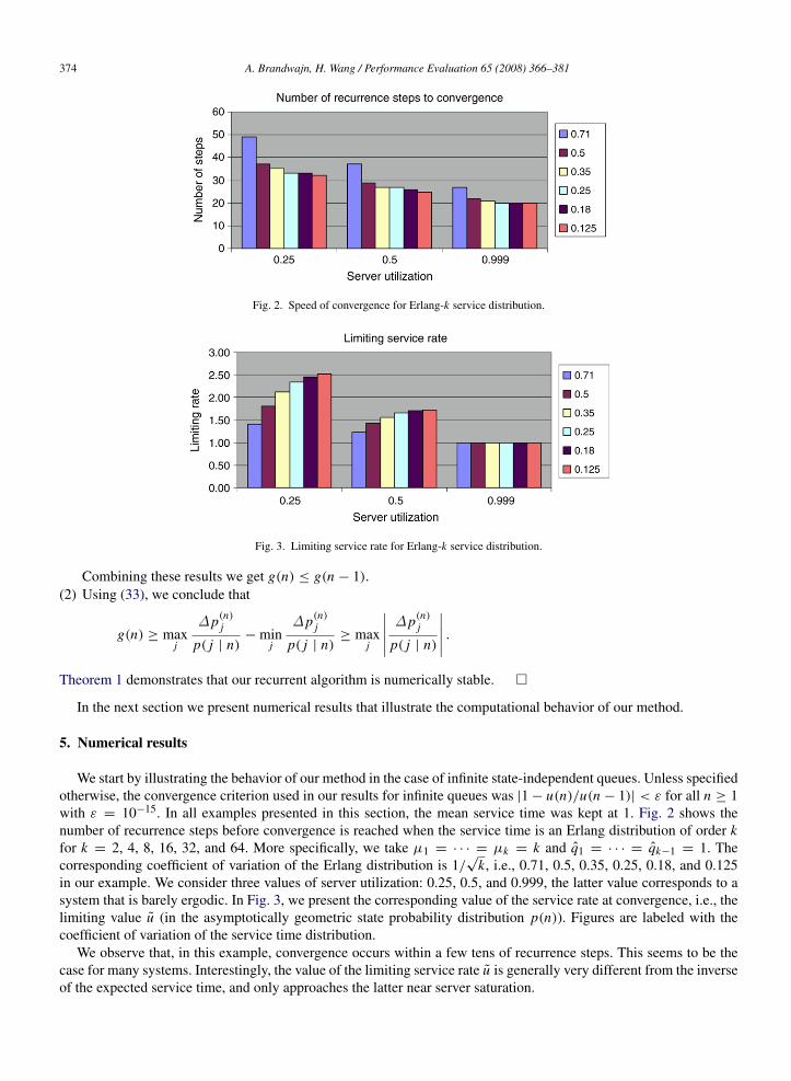
Fig. 2. Speed of convergence for Erlang-k service distribution.

Fig. 3. Limiting service rate for Erlang-k service distribution.

Combining these results we get g(n) ≤ g(n − 1).(2) Using (33), we conclude that

g(n) ≥ maxj

∆p(n)j

p( j | n)− min

j

∆p(n)j

p( j | n)≥ max

j

∣∣∣∣∣ ∆p(n)j

p( j | n)

∣∣∣∣∣ .Theorem 1 demonstrates that our recurrent algorithm is numerically stable. �

In the next section we present numerical results that illustrate the computational behavior of our method.

5. Numerical results

We start by illustrating the behavior of our method in the case of infinite state-independent queues. Unless specifiedotherwise, the convergence criterion used in our results for infinite queues was |1 − u(n)/u(n − 1)| < ε for all n ≥ 1with ε = 10−15. In all examples presented in this section, the mean service time was kept at 1. Fig. 2 shows thenumber of recurrence steps before convergence is reached when the service time is an Erlang distribution of order kfor k = 2, 4, 8, 16, 32, and 64. More specifically, we take µ1 = · · · = µk = k and q1 = · · · = qk−1 = 1. Thecorresponding coefficient of variation of the Erlang distribution is 1/

√k, i.e., 0.71, 0.5, 0.35, 0.25, 0.18, and 0.125

in our example. We consider three values of server utilization: 0.25, 0.5, and 0.999, the latter value corresponds to asystem that is barely ergodic. In Fig. 3, we present the corresponding value of the service rate at convergence, i.e., thelimiting value u (in the asymptotically geometric state probability distribution p(n)). Figures are labeled with thecoefficient of variation of the service time distribution.

We observe that, in this example, convergence occurs within a few tens of recurrence steps. This seems to be thecase for many systems. Interestingly, the value of the limiting service rate u is generally very different from the inverseof the expected service time, and only approaches the latter near server saturation.

A. Brandwajn, H. Wang / Performance Evaluation 65 (2008) 366–381 375

Fig. 4. Example of slower convergence.

Fig. 5. Limiting service rate for slower convergence case.

Although convergence to the limiting service rate value tends to occur rapidly for many systems, there are caseswhen considerably more recurrence steps are needed to achieve the stringent convergence level we used. Fig. 4shows the number of recurrence steps in one of the worst cases we have encountered. The Coxian service timedistribution used in this example corresponds to the following parameters: k = 9, µ1 = 2, µ2 = · · · µk = 2(k − 1)q1,q2 = · · · = qk−1 = 1, and the values of q1 are 0.1, 0.01 and 0.001. The resulting coefficient of variation of the servicetime distribution is 1.68, 5.30, and 16.77, respectively, and we use it to label the results. In Fig. 5, we have representedthe corresponding limiting service rates.

We observe that the number of iteration steps needed to satisfy the specified convergence criterion reaches 2500 inthis case.

Note that although the number of recurrence steps in this example increases with the coefficient of variation of theservice time distribution, other high variability distributions exhibit much faster convergence. Figs. 6 and 7 show theresults for a two-stage Coxian with µ1 = 2 and the following sets of parameter values for the second stage and theprobability that stage 2 will follow the completion of stage 1:

set 1: µ2 = 0.3, q1 = 0.15;

set 2: µ2 = 0.1, q1 = 0.05;

set 3: µ2 = 0.01, q1 = 0.05;

set 4: µ2 = 0.001, q1 = 0.0005.

The resulting coefficient of variation is 1.83, 3.16, 10, and 31.62, respectively.Here we observe that the number of recurrence steps remains below one hundred even for the highest variability

case and very close to server saturation. As before, the limiting service rate is quite different from the inverse ofthe mean service time (1, in our case), except close to saturation. Interestingly, for the high variability distribution

376 A. Brandwajn, H. Wang / Performance Evaluation 65 (2008) 366–381

Fig. 6. Speed of convergence for high variability distribution.

Fig. 7. Limiting service rate for high variability distribution.

Fig. 8. Convergence speed versus convergence stringency.

the limiting service rate value u is lower than the inverse of the mean service time (unlike for the Erlang servicedistribution).

While the value of ε in the convergence criterion used in our examples yields accurate results both for the expectednumber in the system and for selected state probabilities, it may seem rather stringent. In our next example, we studythe influence of the convergence stringency on the number of recurrence steps. The results shown in Fig. 8 have beenobtained for a service time distribution similar to that used in Figs. 4 and 5, except that the total number of stages inthe Coxian distribution is 7. The coefficient of variation of the service time distribution is 17.08. The results in Fig. 8are labeled by the server utilization.

A. Brandwajn, H. Wang / Performance Evaluation 65 (2008) 366–381 377

Fig. 9. Expected number of customers in finite source system.

Fig. 10. Probability server is idle in finite source system.

We notice that, at higher server utilization levels, the convergence stringency may have an important effect on thenumber of recurrence steps required. For the convergence criterion used in these examples, |1 − u(n)/u(n − 1)| < ε

for all n ≥ 1, it has been our experience that ε = 10−13 is sufficient to achieve accurate results for most systems withserver utilization of up to 0.98. For server utilizations not exceeding 0.7, ε = 10−11 tends to be sufficient. Note thatfor many systems the number of recurrence steps to convergence is quite low even with more stringent values for ε,and the solution time in all cases is negligible. The computational effort at each recurrence step is minimal. Note alsothat the storage requirements of our approach are very low. If we embed the recurrence steps inside the computationof state probabilities p(n) for increasing values of n, there is no need to store more than the last set of the conditionalprobabilities p(i | n) and the last two values of the service rate u(n). It is also sufficient to store only the values of p(n)

(and any derived quantities) one is interested in. Additionally, we note that, even in the cases where a larger number ofrecurrence steps is needed, we have not encountered numerical problems. Since we know the limiting service rate ufrom the solution of Eqs. (24) and (25), we can double check for any loss of accuracy when the recurrent computationof u(n) ends due to convergence.

As a last example, we consider a system with state-dependent arrivals where λ(n) = (N − n)α. This form of thearrival rate corresponds to a set of N customers each generating a request with rate α. The results shown in Figs. 9 and10 pertain to a system with N = 100 and the nine-stage high variability service time distribution used in Figs. 4 and5. In this finite-source example, we consider more values for q1: 0.5, 0.1, 0.05, 0.01, 0.005, and 0.001. The resultingcoefficient of variation for the service time distribution ranges from 0.75 to 16.77, and is used as a label in Figs. 8 and 9.

Fig. 9 displays the expected number of customers in the system as a function of the maximum arrival rate Nα.Fig. 10 shows the corresponding probability that the server is idle in such a system versus the same maximum arrivalrate.

It is interesting to note the effect of service time variability on the expected number of customers in the system,as well as on the probability that the system is idle. As the coefficient of variation of the service time distributionincreases so does the probability that the server is idle. This effect becomes more visible as the maximum arrival rate

378 A. Brandwajn, H. Wang / Performance Evaluation 65 (2008) 366–381

increases. The expected number of customers increases with service time variability but the relative increase withservice time variability becomes smaller as the arrival rate increases.

Overall, in all the examples we studied, we have found the proposed method to be numerically well behaved, andgenerally very fast. Additionally, our method is quite easy to implement in a language like C, C++, Java or FORTRAN,with minimal memory space requirements.

6. Conclusion

We have proposed an approach, believed to be novel, to the solution of M /G/1-like queues in which the service timedistribution is represented by a Coxian series of memoryless stages. Our method is based on elementary conditionalprobabilities, and provides a simple, computationally efficient and stable recurrence that allows us to obtain state-dependent service rates, and, hence, the steady-state queue length distribution. Unlike existing methods, the proposedapproach does not rely on the use of matrix-geometric techniques or stochastic complementation. It can handlegeneralized queues in which both the arrival rates and the parameters of the service time distribution, including theprobabilities of moving from stage to stage, may be state dependent. Our method can be applied to both finite andinfinite M /G/1-like queues. We believe that our method combines conceptual simplicity, ease of implementation andcomputational efficiency.

In the case of an infinite, state-independent queue, the explicit product form of the queue length distribution in ourmethod allows us to show that it is asymptotically geometric. Additionally, we have given a simple set of equations thatdefines the limiting service rate for this geometric distribution, and we have presented a simple fixed-point iterationto solve it.

We have provided a proof of the numerical stability of our algorithm in the general case, and a proof of itsconvergence to the unique non-negative fixed point in the case of a state-independent infinite queue. We have includedseveral examples to illustrate the performance of our method in the case of an infinite M /G/1-like queue. We haveconsidered both low and high service time variability, and server utilizations ranging from low to very close tosaturation. Our results for infinite queues suggest that, in general, only a moderate number of recurrence steps isneeded to reach the limiting service rate with high accuracy. In many cases, just a few tens of recurrence steps may besufficient. We have also included an example to illustrate the results obtained with our method in the case of a finitenumber of customers and state-dependent arrivals.

The proposed method is in general fast, very thrifty in terms of memory space requirements, conceptually simple,and easy to implement. It is stable even for systems with server utilization very close to saturation. Its simplicityand numeric stability should make it attractive to performance analysts. An extension of this approach to M /G/1-likesystems with service interruptions is under study.

Acknowledgments

The authors wish to thank the anonymous referees for their remarks and suggestions which helped improve thispaper.

Appendix A

A.1. Proof of lemmas

Proof of Lemma 2. Suppose max j∆c(n)

jc j (n)

is attained at j = m. At i = m, we write (32) as[∆c(n)

m

cm(n)

]cm(n)[λ(n) + µm(n)] −

[∆c(n)

m−1

cm−1(n)

]cm−1(n)µm−1(n)qm−1(n) =

[∆p(n−1)

m

p(m | n − 1)

]p(m | n − 1)

which leads to[∆c(n)

m

cm(n)

]{cm(n)[λ(n) + µm(n)] − cm−1(n)µm−1(n)qm−1(n)} ≤

[∆p(n−1)

m

p(m | n − 1)

]p(m | n − 1).

A. Brandwajn, H. Wang / Performance Evaluation 65 (2008) 366–381 379

On the other hand, at i = m, (31) becomes

cm(n)[λ(n) + µm(n)] − cm−1(n)µm−1(n)qm−1(n) = p(m | m − 1).

Combining these two results, we obtain

maxj

∆c(n)j

c j (n)=

∆c(n)m

cm(n)≤

∆p(n−1)m

p(m | n − 1)≤ max

j

∆p(n−1)j

p( j | n − 1).

Using an analogous approach, we can show that

minj

∆c(n)j

c j (n)≥ min

j

∆p(n−1)j

p( j | n − 1). �

Proof of Lemma 3.

∆u(n) = u(n) − u(n)

=

1 − λ(n)k∑

j=1b j (n)

k∑j=1

[c j (n) + ∆c(n)j ]

−

1 − λ(n)k∑

j=1b j (n)

k∑j=1

c j (n)

=

−

(1 − λ(n)

k∑j=1

b j (n)

)(k∑

j=1∆c(n)

j

)(

k∑j=1

c j (n)

)(k∑

j=1c j (n) +

k∑j=1

∆c(n)j

) = −u(n)∆β(n)

1 + ∆β(n)

∆p(n)i = p(i | n) − p(i | n)

= [u(n) + ∆u(n)] [ci (n) + ∆c(n)i ] − u(n)ci (n)

= u(n)∆c(n)i + ∆u(n)[ci (n) + ∆c(n)

i ]

= u(n)

[∆c(n)

i −∆β(n)

1 + ∆β(n)[ci (n) + ∆c(n)

i ]

]=

u(n)

1 + ∆β(n)[∆c(n)

i − ∆β(n)ci (n)]. �

Proof of Lemma 4. Using (29) and the fact that p( j |n)−λb jp( j |n)

≤ 1 − λ min j b j = α, we obtain

maxj

∆p(n)j

p( j | n)= max

j

(p( j | n) − λb j

p( j | n)·

∆p(n)j

u(n)ci (n)

)≤ α max

j

∆p(n)j

u(n)ci (n)

minj

∆p(n)j

p( j | n)= min

j

(p( j | n) − λ b j

p( j | n)·

∆p(n)j

u(n)ci (n)

)≥ α min

j

∆p(n)j

u(n)ci (n).

Substituting into function g(n) yields

g(n) ≤ α

maxj

∆p(n)j

u(n)c j (n)− min

j

∆p(n)j

u(n)c j (n)

1 + minj

∆p(n)j

u(n)c j (n)

.

Then g(n) ≤ αg(n − 1) follows from the proof of Theorem 1. �

380 A. Brandwajn, H. Wang / Performance Evaluation 65 (2008) 366–381

A.2. Convergence to fixed point for infinite state-independent queue

Consider now the infinite state-independent queue of Section 3. For an infinite state-independent queue, allparameters are independent of n. As a results, the coefficients bi defined in (30) are also independent of n. Letα = 1 − λ min j b j . From Lemma 1 we get 0 < α < 1, and we have

Lemma 4. For an infinite state-independent queue, g(n) satisfies

g(n) ≤ αg(n − 1).

Proof of Lemma 4. See Appendix A.1. �

For notational convenience, we let Ep(n) = (p(1 | n), p(2 | n), . . . , p(k | n))T . We have

Theorem 2. The sequence { Ep(n), n = 1, 2, . . . , } converges to a unique fixed point.

Proof of Theorem 2. The key to the proof is to view Ep(n + 1) as Ep(n) perturbed:

p( j | n + 1) = p( j | n) + ∆p(n)j .

Using the results of Theorem 1 and Lemma 4, we have

‖ Ep(n + 1) − Ep(n)‖∞ = maxj

|∆p(n)j | ≤ max

j|

∆p(n)j

p( j | n)| ≤ g(n) ≤ αng(1)

and

‖ Ep(N + m) − Ep(N )‖∞ ≤

N+m−1∑n=N

‖ Ep(n + 1) − Ep(n)‖∞ ≤

(N+m−1∑

n=N

αn

)g(1) ≤ αN g(1)

1 − α.

Thus, { Ep(n), n = 1, 2, . . . , } is a Cauchy sequence with respect to the infinity norm, and converges with respect tothis norm to a limit Ep(∞). Since Ep(∞) is the limit of both Ep(n) and Ep(n + 1), it must be a fixed point. �

Now we show that our recurrent algorithm has only one non-negative fixed point. Suppose Ep(n) =

(p(1), p(2), . . . , p(k))T is a fixed point of our recurrent algorithm. Substituting into (28), we have

p(i)(λ + µi ) = p(i − 1)µi−1qi−1 + λδi,1 + p(i)u, where u =

k∑j=1

p( j)µ j q j . (34)

Let us treat u as a parameter and write p(i) as

p(i) = [p(i − 1)µi−1qi−1 + λδi,1]/(λ + µi − u).

To ensure that p(i) is non-negative, we must have u < min j (λ + µ j ). It is clear that for u < min j (λ + µ j ),p(i) is a strictly increasing function of u. When u = 0, summing (34) over all values of i and dividing by λ yields∑k

i=1 p(i) = 1 −1λ

∑ki=1 p(i)µi qi < 1. As u → min j (λ + µ j ),

∑ki=1 p(i) → +∞ > 1. Since

∑ki=1 p(i) is a

continuous and strictly increasing function of u, there is a unique value of u such that∑k

i=1 p(i) = 1 is satisfied. Thismeans that the non-linear equation (34) has a unique non-negative solution.

References

[1] N. Akar, K. Sohraby, An invariant subspace approach in M /G/1 and G/M /1 type Markov chains, Commun. Statist. Stochastic Models 13(1997) 381–416.

[2] A.O. Allen, Probability, Statistics, and Queuing Theory, 2nd edition, Academic Press, 1990.[3] N.G. Bean, P.K. Pollett, P.G. Taylor, Quasistationary distributions for level-dependent quasi-birth-and-death processes, Commun. Statist.

Stochastic Models 16 (2000) 511–541.[4] N.G. Bean, J.-M. Li, P.G. Taylor, Caudal characteristics of QBDs with decomposable phase spaces, in: G. Latouche, P.G. Taylor (Eds.),

Advances in Algorithmic Methods for Stochastic Models, Notable Publications, NJ, 2000, pp. 37–56.[5] D.A. Bini, G. Latouche, B. Meini, Numerical Methods for Structured Markov Chains, Oxford University Press, 2005.

A. Brandwajn, H. Wang / Performance Evaluation 65 (2008) 366–381 381

[6] D. Bini, B. Meini, On the solution of a nonlinear matrix equation arising in queueing problems, SIAM J. Matrix Anal. Appl. 17 (1996)906–926.

[7] D.A. Bini, B. Meini, Improved cyclic reduction for solving queueing problems, Numer. Algorithms 15 (1997) 57–74.[8] D.A. Bini, B. Meini, S. Steffe, B. van Houdt, Structured Markov chain solver: The algorithms, in: Proceedings of the SMCTOOLS Workshop,

Pisa, 2006.[9] D.A. Bini, B. Meini, S. Steffe, B. van Houdt, Structured Markov chain solver: Software tools, in: Proceedings of the SMCTOOLS Workshop,

Pisa, 2006.[10] L.W. Bright, P.G. Taylor, Calculating the equilibrium distribution in level dependent quasi-birth-and-death processes, Commun. Statist.

Stochastic Models 11 (1995) 497–525.[11] W. Bux, U. Herzog, The phase concept: Approximation of measured data and performance analysis, in: Proceedings of the International

Symposium on Computer Performance Modeling, Measurement and Evaluation, North Holland, Yorktown Heights, NY, 1977, pp. 23–38.[12] D.R. Cox, Walter L. Smith, Queues, John Wiley, New York, 1961.[13] M. Faddy, Penalised maximum likelihood estimation of the parameters in a coxian phase-type distribution, in: Matrix-Analytic Methods:

Theory and Application: Proceedings of the Fourth International Conference, Adelaide, Australia, 2002, pp. 107–114.[14] P. Gaver, A. Jacobs, G. Latouche, Finite birth-and-death models in randomly changing environments, Adv. Appl. Probab. 16 (1984) 715–731.[15] C. Knessl, B. Matkowsky, Z. Schuss, C. Tier, Asymptotic analysis of a state-dependent M /G/1 queueing system, SIAM J. Appl. Math. 46

(1986) 483–505.[16] C. Knessl, C. Tier, B. Matkowsky, Z. Shuss, A state-dependent GI/G/1 queue, Eur. J. Appl. Math. 5 (1994) 217–241.[17] G. Latouche, Newton’s iteration for non-linear equations in Markov chains, IMA J. Numer. Anal. 14 (1994) 583–598.[18] G. Latouche, V. Ramaswami, A logarithmic reduction algorithm for quasi-birth-and-death processes, J. Appl. Probab. 30 (1993) 650–674.[19] G. Latouche, V. Ramaswami, Introduction to matrix analytic methods in stochastic modeling, in: ASA-SIAM Series on Statistics and Applied

Probability, Society for Industrial and Applied Mathematics (SIAM), Philadelphia, PA, 1999.[20] S. McLean, M. Faddy, P. Millard, Using Markov models to assess the performance of a health and community care system, in: Proceedings

of the 19th IEEE Symposium on Computer-Based Medical Systems, 2006, pp. 777–782.[21] B. Meini, Solving M /G/1-type Markov chains: Recent advances and applications, Commun. Statist. Stochastic Models 14 (1998) 479–496.[22] B. Meini, An improved FFT-based version of Ramaswami’s formula, Commun. Statist. Stochastic Models 13 (1997) 223–238.[23] M.F. Neuts, Matrix-geometric Solutions in Stochastic Models, John Hopkins University Press, Baltimore, MD, 1981.[24] M.F. Neuts, Structured Stochastic Matrices of M /G/1-type and Their Applications, Marcel Dekker, New York, NY, 1989.[25] V. Ramaswami, A stable recursion for the steady state vector in Markov chains of M /G/1-type, Commun. Statist. Stochastic Models 4 (1988)

183–189.[26] V. Ramaswami, P.G. Taylor, Some properties of the rate operators in level dependent quasi-birth-and-death processes with a countable number

of phases, Commun. Statist. Stochastic Models 12 (1996) 143–164.[27] A. Riska, E. Smirni, Exact aggregate solutions for M /G/1-type Markov processes, in: Proceedings of the ACM SIGMETRICS Conference,

Marina Del Rey, CA, USA, June 2002, pp. 86–96.[28] A. Riska, E. Smirni, M /G/1-type Markov processes: A tutorial, in: Performance Evaluation of Complex Computer Systems: Techniques and

Tools, in: LNCS, vol. 2549, Springer Verlag, 2002, pp. 36–63.[29] Y. Sasaki, H. Imai, M. Tsunoyama, et al., Approximation of probability distribution functions by Coxian distribution to evaluate multimedia

systems, Systems and Computers in Japan 35 (2) (2004) 16–24.[30] A. Stathopoulos, A. Riska, Z. Hua, et al., Bridging ETAQA and Ramaswami’s formula for the solution of M /G/1-type processes, Performance

Eval. 62 (1–4) (2005) 331–348.[31] Q. Ye, On Latouche–Ramaswami’s logarithmic reduction algorithm for quasi-birth-and-death processes, Commun. Statist. Stochastic Models

18 (2002) 449–467.