Conditional Probability And the odds ratio and risk ratio as conditional probability

Conditional Probability

And the odds ratio and risk ratio as conditional probability

Today’s lecture Probability trees Statistical independence Joint probability Conditional probability Marginal probability Bayes’ Rule Risk ratio Odds ratio

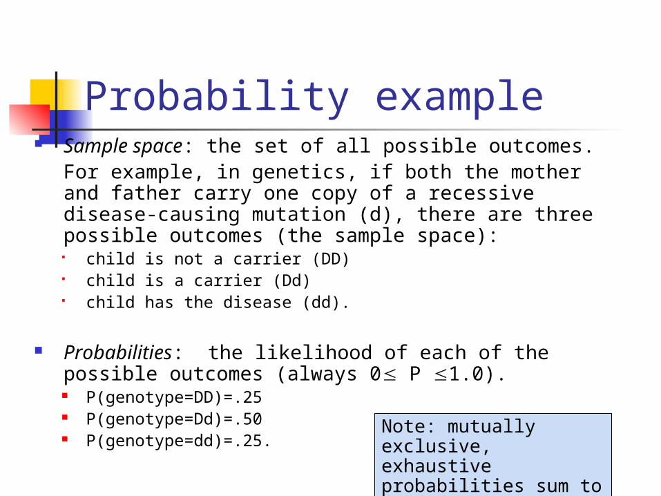
Probability example Sample space: the set of all possible outcomes.

For example, in genetics, if both the mother and father carry one copy of a recessive disease-causing mutation (d), there are three possible outcomes (the sample space): child is not a carrier (DD) child is a carrier (Dd) child has the disease (dd).

Probabilities: the likelihood of each of the possible outcomes (always 0 P 1.0). P(genotype=DD)=.25 P(genotype=Dd)=.50 P(genotype=dd)=.25.

Note: mutually exclusive, exhaustive probabilities sum to 1.

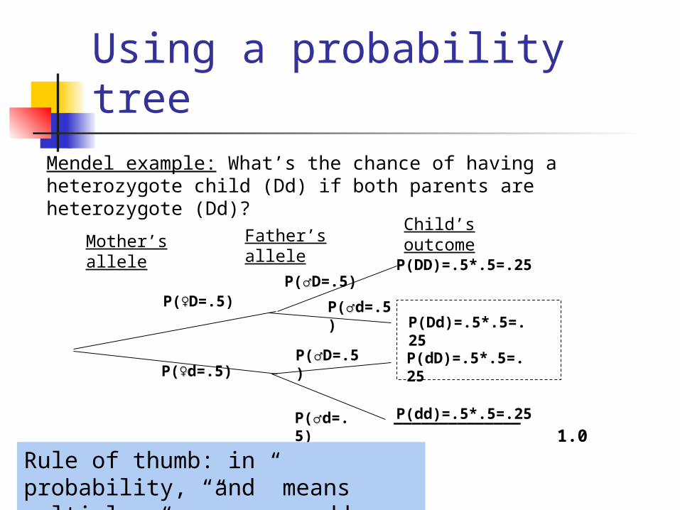
Using a probability tree

P(♀♀D=.5)

P(♀♀d=.5)

Mother’s allele

P(♂♂D=.5)

P(♂♂d=.5)

P(♂♂D=.5)

P(♂♂d=.5)

Father’s allele

______________ 1.0

P(DD)=.5*.5=.25

P(Dd)=.5*.5=.25

P(dD)=.5*.5=.25

P(dd)=.5*.5=.25

Child’s outcome

Rule of thumb: in probability, “and” means multiply, “or” means add

Mendel example: What’s the chance of having a heterozygote child (Dd) if both parents are heterozygote (Dd)?

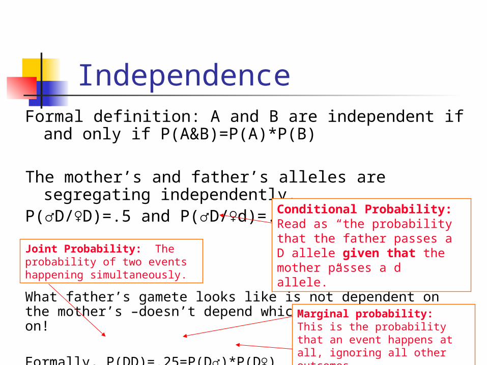
IndependenceFormal definition: A and B are independent if and only

if P(A&B)=P(A)*P(B)

The mother’s and father’s alleles are segregating independently.

P(♂D/♀D)=.5 and P(♂D/♀d)=.5

What father’s gamete looks like is not dependent on the mother’s –doesn’t depend which branch you start on!

Formally, P(DD)=.25=P(D♂)*P(D♀)

Conditional Probability: Read as “the probability that the father passes a D allele given that the mother passes a d allele.”Joint Probability: The probability

of two events happening simultaneously.

Marginal probability: This is the probability that an event happens at all, ignoring all other outcomes.

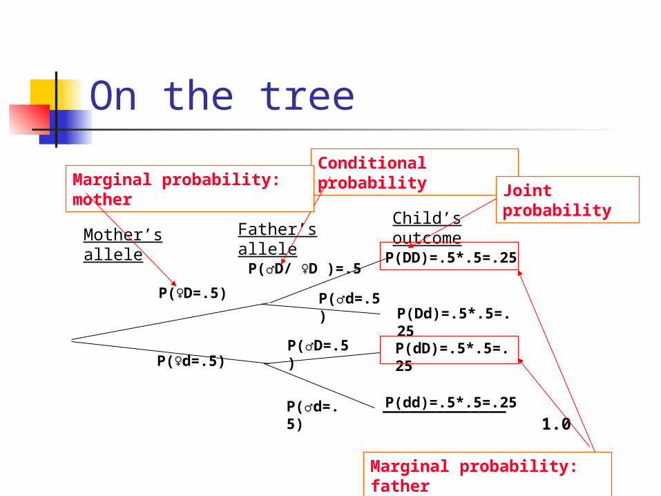
On the tree

P(♀♀D=.5)

P(♀♀d=.5)

Mother’s allele

P(♂♂D/ ♀♀D )=.5

P(♂♂d=.5)

P(♂♂D=.5)

P(♂♂d=.5)

Father’s allele

______________ 1.0

P(DD)=.5*.5=.25

P(Dd)=.5*.5=.25

P(dD)=.5*.5=.25

P(dd)=.5*.5=.25

Child’s outcome

Conditional probabilityMarginal probability: mother

Joint probability

Marginal probability: father

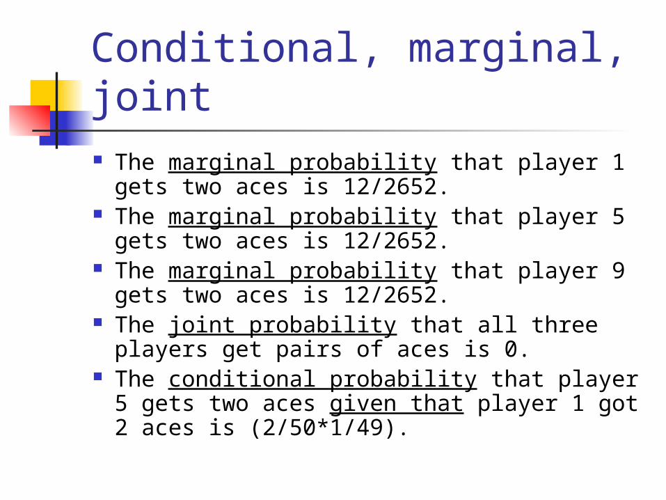
Conditional, marginal, joint The marginal probability that player 1 gets

two aces is 12/2652. The marginal probability that player 5 gets

two aces is 12/2652. The marginal probability that player 9 gets

two aces is 12/2652. The joint probability that all three players

get pairs of aces is 0. The conditional probability that player 5

gets two aces given that player 1 got 2 aces is (2/50*1/49).

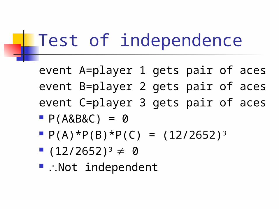
Test of independence

event A=player 1 gets pair of acesevent B=player 2 gets pair of acesevent C=player 3 gets pair of aces P(A&B&C) = 0 P(A)*P(B)*P(C) = (12/2652)3

(12/2652)3 0 Not independent

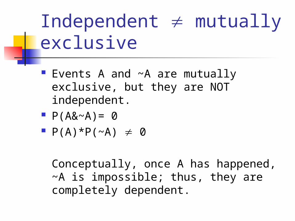
Independent mutually exclusive Events A and ~A are mutually exclusive,

but they are NOT independent. P(A&~A)= 0 P(A)*P(~A) 0

Conceptually, once A has happened, ~A is impossible; thus, they are completely dependent.

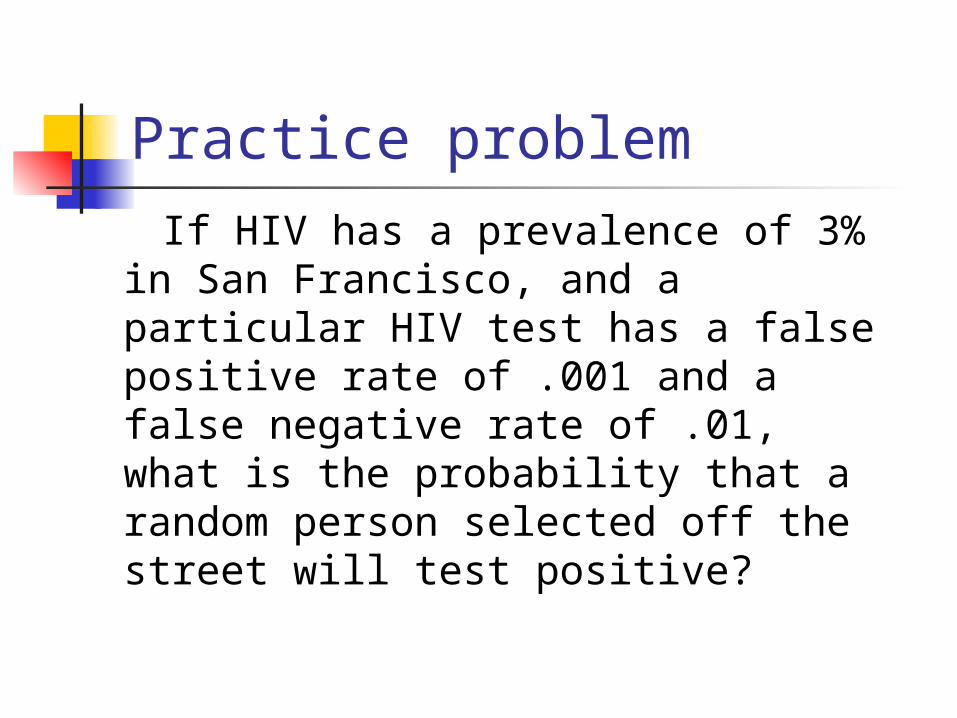
Practice problem

If HIV has a prevalence of 3% in San Francisco, and a particular HIV test has a false positive rate of .001 and a false negative rate of .01, what is the probability that a random person selected off the street will test positive?

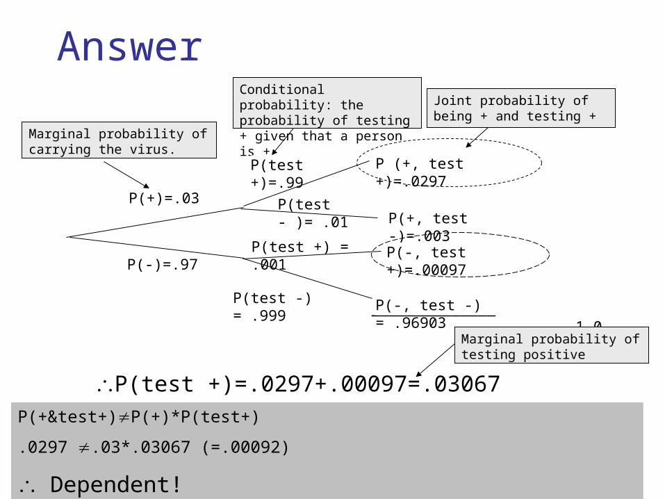
Answer

______________ 1.0

P (+, test +)=.0297

P(+, test -)=.003

P(-, test +)=.00097

P(-, test -) = .96903

P(test +)=.0297+.00097=.03067

Marginal probability of carrying the virus.

Joint probability of being + and testing +

P(+&test+)P(+)*P(test+)

.0297 .03*.03067 (=.00092)

Dependent!

Marginal probability of testing positive

Conditional probability: the probability of testing + given that a person is +

P(+)=.03

P(-)=.97

P(test +)=.99

P(test - )= .01

P(test +) = .001

P(test -) = .999

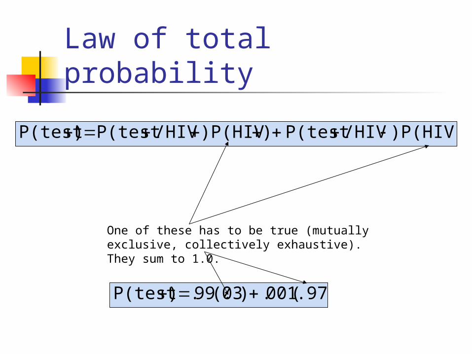
Law of total probability

)P(HIV-)/HIVP(test ))P(HIV/HIVP(test )P(test

.97)(001.)03(.99.)P(test

One of these has to be true (mutually exclusive, collectively exhaustive). They sum to 1.0.

Law of total probability

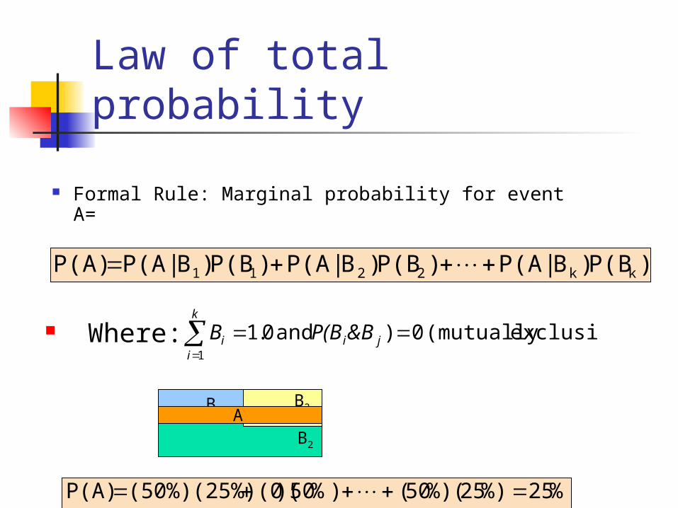
Formal Rule: Marginal probability for event A=

)P(B)B|P(A)P(B)B|P(A)P(B)B|P(A P(A) kk2211

exclusive)(mutually 0) and 0.11

ji

k

ii &BP(BB

B2

B3 B1

Where:

%25%)25%)(50()%50)((0(50%)(25%) P(A)

A

Example 2

A 54-year old woman has an abnormal mammogram; what is the chance that she has breast cancer?

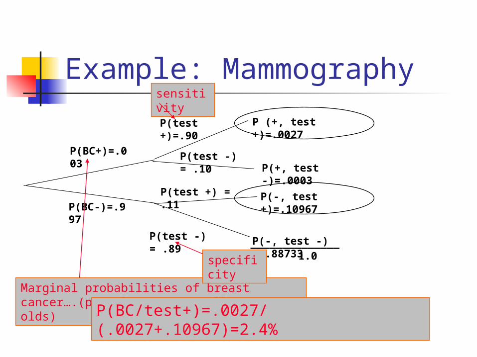
Example: Mammography

______________1.0

P(test +)=.90

P(BC+)=.003

P(BC-)=.997

P(test -) = .10

P(test +) = .11

P (+, test +)=.0027

P(+, test -)=.0003

P(-, test +)=.10967

P(-, test -) = .88733P(test -) = .89

Marginal probabilities of breast cancer….(prevalence among all 54-year olds)

sensitivity

specificity

P(BC/test+)=.0027/(.0027+.10967)=2.4%

Bayes’ rule

Bayes’ Rule: derivation

)(

)&()/(

BP

BAPBAP

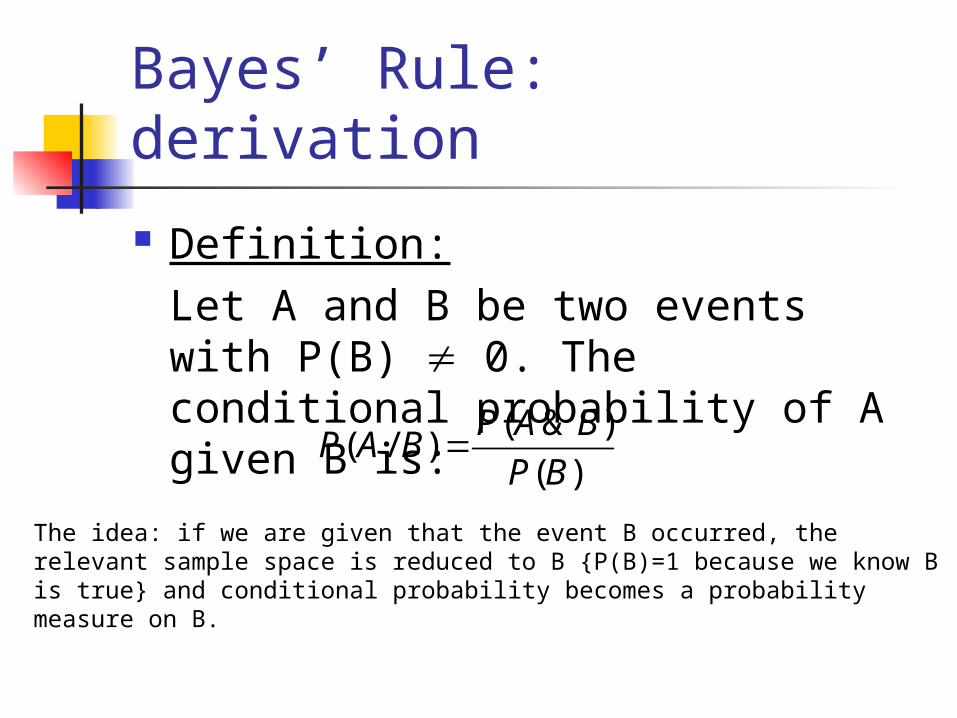
Definition:Let A and B be two events with P(B) 0. The conditional probability of A given B is:

The idea: if we are given that the event B occurred, the relevant sample space is reduced to B {P(B)=1 because we know B is true} and conditional probability becomes a probability measure on B.

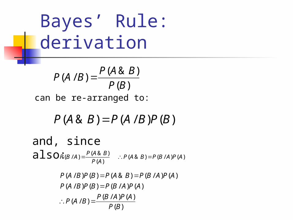
Bayes’ Rule: derivation

can be re-arranged to:

)()/()&( BPBAPBAP

)()/()&( )(

)&()/( APABPBAP

AP

BAPABP

)(

)()/()/(

)()/()()/(

)()/()&()()/(

BP

APABPBAP

APABPBPBAP

APABPBAPBPBAP

)(

)&()/(

BP

BAPBAP

and, since also:

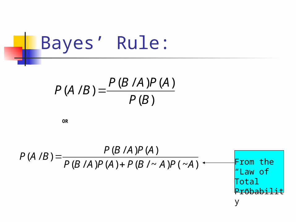
Bayes’ Rule:

)(

)()/()/(

BP

APABPBAP

From the “Law of Total Probability”

OR

)(~)~/()()/(

)()/()/(

APABPAPABP

APABPBAP

Bayes’ Rule:

Why do we care?? Why is Bayes’ Rule useful?? It turns out that sometimes it is very

useful to be able to “flip” conditional probabilities. That is, we may know the probability of A given B, but the probability of B given A may not be obvious. An example will help…

In-Class Exercise

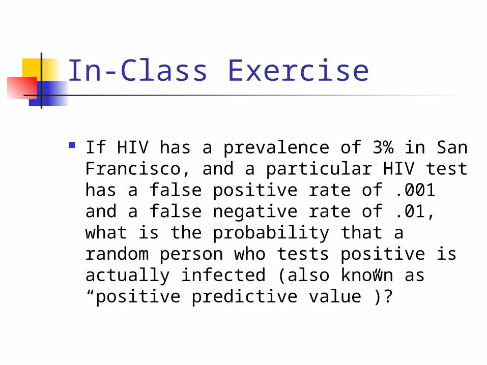
If HIV has a prevalence of 3% in San Francisco, and a particular HIV test has a false positive rate of .001 and a false negative rate of .01, what is the probability that a random person who tests positive is actually infected (also known as “positive predictive value”)?

Answer: using probability tree

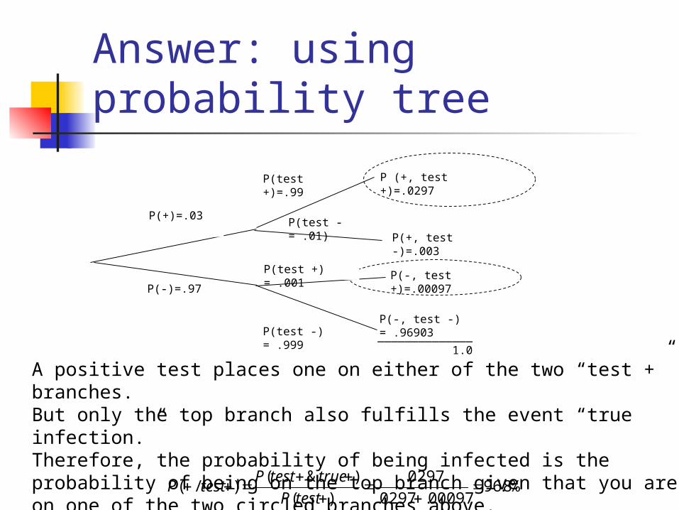
______________ 1.0

P(test +)=.99

P(+)=.03

P(-)=.97

P(test - = .01)

P(test +) = .001

P (+, test +)=.0297

P(+, test -)=.003

P(-, test +)=.00097

P(-, test -) = .96903P(test -) = .999

A positive test places one on either of the two “test +” branches. But only the top branch also fulfills the event “true infection.” Therefore, the probability of being infected is the probability of being on the top branch given that you are on one of the two circled branches above.

%8.9600097.0297.

0297.

)(

)&()/(

testP

truetestPtestP

Answer: using Bayes’ rule

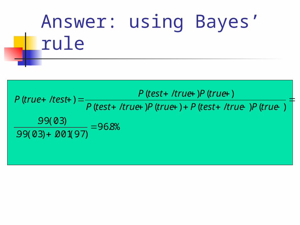
%8.96)97(.001.)03(.99.

)03(.99.

)()/()()/(

)()/()/(

truePtruetestPtruePtruetestP

truePtruetestPtesttrueP

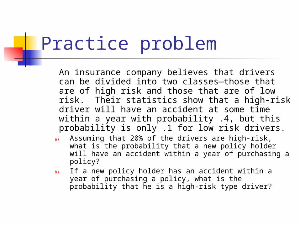
Practice problemAn insurance company believes that drivers can be divided into two classes—those that are of high risk and those that are of low risk. Their statistics show that a high-risk driver will have an accident at some time within a year with probability .4, but this probability is only .1 for low risk drivers.

a) Assuming that 20% of the drivers are high-risk, what is the probability that a new policy holder will have an accident within a year of purchasing a policy?

b) If a new policy holder has an accident within a year of purchasing a policy, what is the probability that he is a high-risk type driver?

Answer to (a)

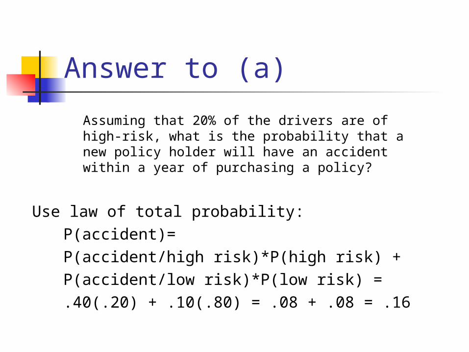
Assuming that 20% of the drivers are of high-risk, what is the probability that a new policy holder will have an accident within a year of purchasing a policy?

Use law of total probability:P(accident)=P(accident/high risk)*P(high risk) + P(accident/low risk)*P(low risk) = .40(.20) + .10(.80) = .08 + .08 = .16

Answer to (b)

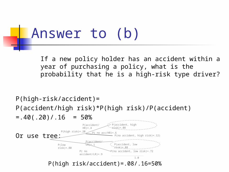
If a new policy holder has an accident within a year of purchasing a policy, what is the probability that he is a high-risk type driver?

P(high-risk/accident)=P(accident/high risk)*P(high risk)/P(accident)=.40(.20)/.16 = 50%

Or use tree:

P(accident/LR)=.1

______________1.0

P( no acc/HR)=.6

P(accident/HR)=.4

P(high risk)=.20

P(accident, high risk)=.08

P(no accident, high risk)=.12)

P(accident, low risk)=.08P(low risk)=.80

P( no accident/LR)=.9

P(no accident, low risk)=.72

P(high risk/accident)=.08/.16=50%

Fun example/bad investment

http://www.cellulitedx.com/

http://www.cellulitedx.com/

Conditional Probability for Epidemiology:

The odds ratio and risk ratio as conditional

probability

The Risk Ratio and the Odds Ratio as conditional probability

In epidemiology, the association between a risk factor or protective factor (exposure) and a disease may be evaluated by the “risk ratio” (RR) or the “odds ratio” (OR). Both are measures of “relative risk”—the general concept of comparing disease risks in exposed vs. unexposed individuals.

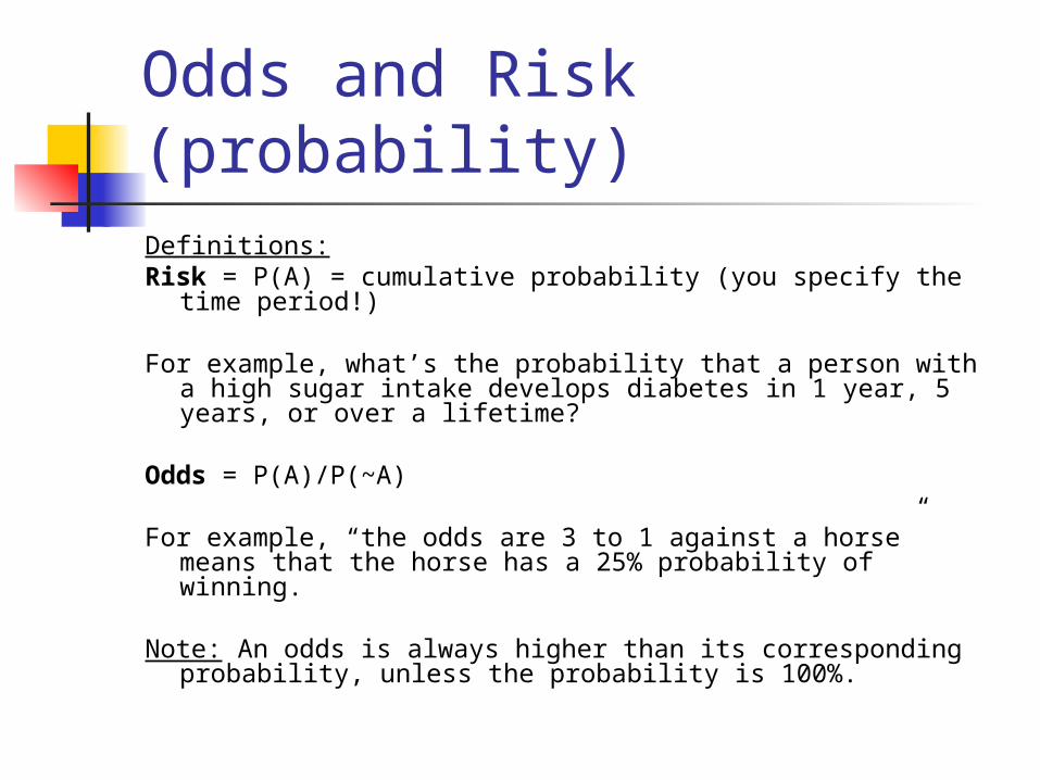
Odds and Risk (probability)Definitions:Risk = P(A) = cumulative probability (you specify the time

period!)

For example, what’s the probability that a person with a high sugar intake develops diabetes in 1 year, 5 years, or over a lifetime?

Odds = P(A)/P(~A)

For example, “the odds are 3 to 1 against a horse” means that the horse has a 25% probability of winning.

Note: An odds is always higher than its corresponding probability, unless the probability is 100%.

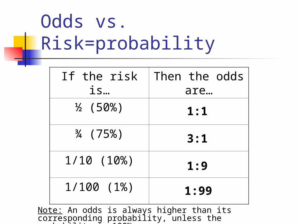
Odds vs. Risk=probability

If the risk is… Then the odds are…

½ (50%)

¾ (75%)

1/10 (10%)

1/100 (1%)

Note: An odds is always higher than its corresponding probability, unless the probability is 100%.

1:1

3:1

1:9

1:99

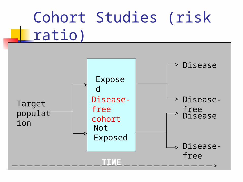
Cohort Studies (risk ratio)

Target population

Exposed

Not Exposed

Disease-free cohort

Disease

Disease-free

Disease

Disease-free

TIME

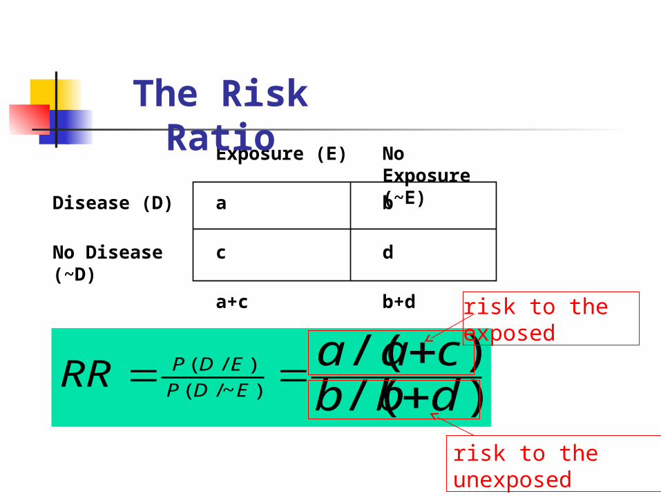
Exposure (E) No Exposure (~E)

Disease (D) a b

No Disease (~D) c d

a+c b+d

)/()/(

)~/(

)/(

dbbcaa

EDP

EDPRR

risk to the exposed

risk to the unexposed

The Risk Ratio

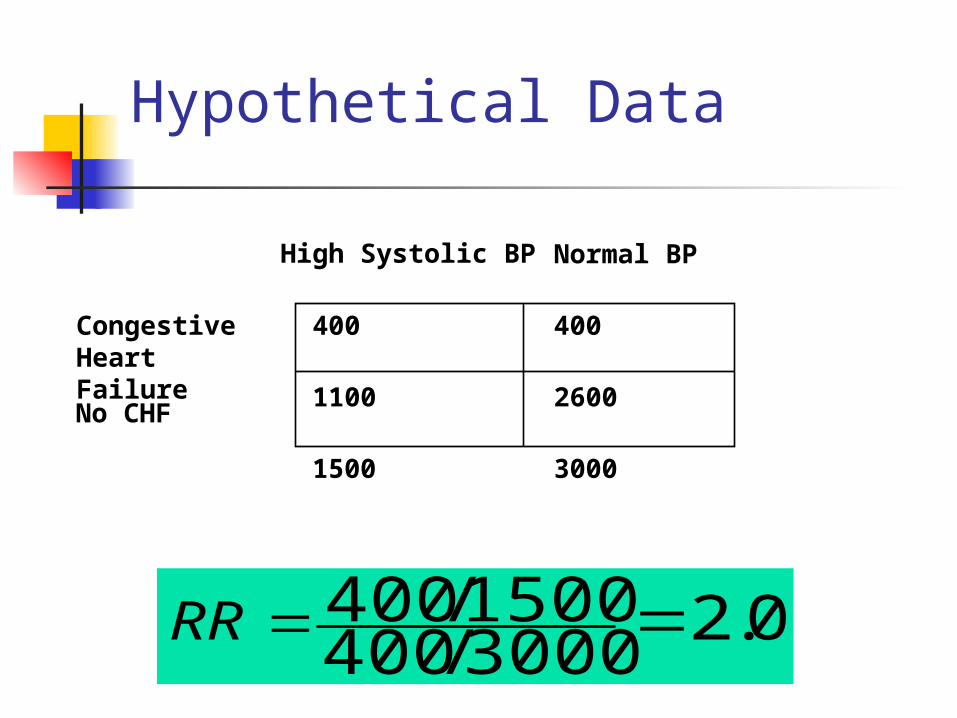
400 400

1100 2600

0.23000/4001500/400 RR

Hypothetical Data

Normal BP

Congestive Heart Failure

No CHF

1500 3000

High Systolic BP

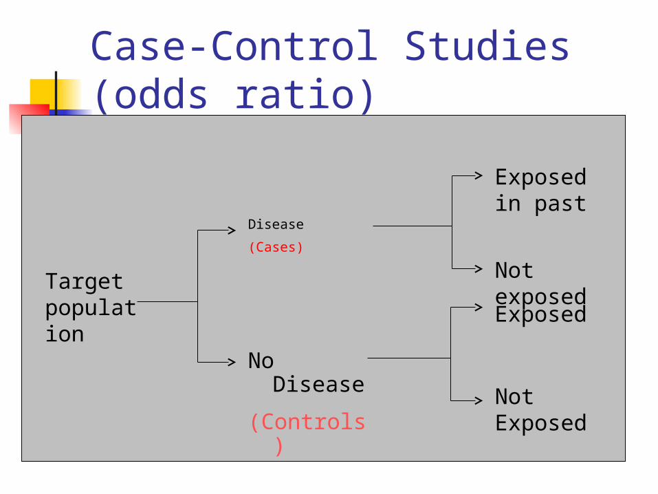
Target population

Exposed in past

Not exposed

Exposed

Not Exposed

Case-Control Studies (odds ratio)

Disease

(Cases)

No Disease

(Controls)

Case-control study example:

You sample 50 stroke patients and 50 controls without stroke and ask about their smoking in the past.

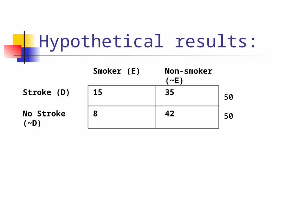
Hypothetical results:

Smoker (E) Non-smoker (~E)

Stroke (D) 15 35

No Stroke (~D) 8 42

50

50

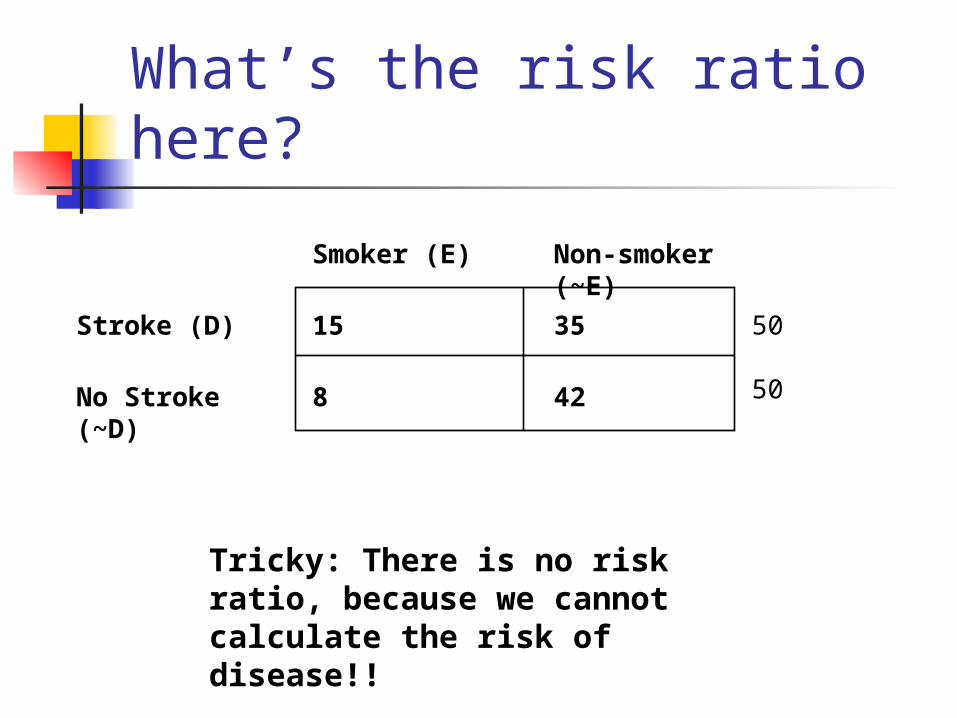
What’s the risk ratio here?

50

50

Tricky: There is no risk ratio, because we cannot calculate the risk of disease!!


Stroke (D) 15 35

No Stroke (~D) 8 42

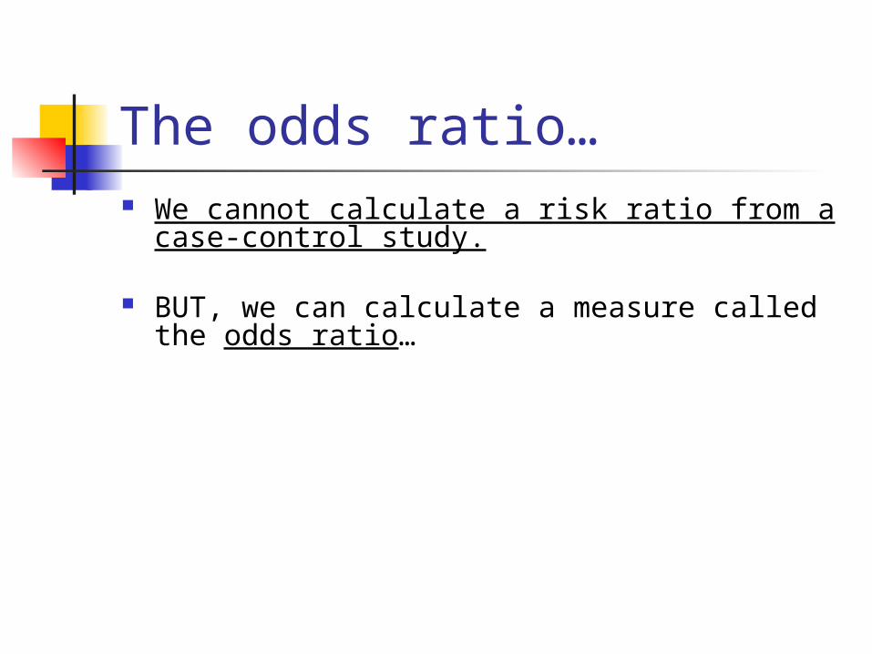
The odds ratio… We cannot calculate a risk ratio from a case-

control study.

BUT, we can calculate a measure called the odds ratio…

Smoker (E) Smoker (~E)

Stroke (D) 15 35

No Stroke (~D)

8 42

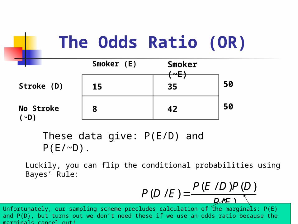
The Odds Ratio (OR)

Luckily, you can flip the conditional probabilities using Bayes’ Rule:

)(

)()/()/(

EP

DPDEPEDP

Unfortunately, our sampling scheme precludes calculation of the marginals: P(E) and P(D), but turns out we don’t need these if we use an odds ratio because the marginals cancel out!

50

50

These data give: P(E/D) and P(E/~D).

bc

ad

dcba

ORDEPDEP

DEPDEP

)~/(~

)~/(

)/(~)/(

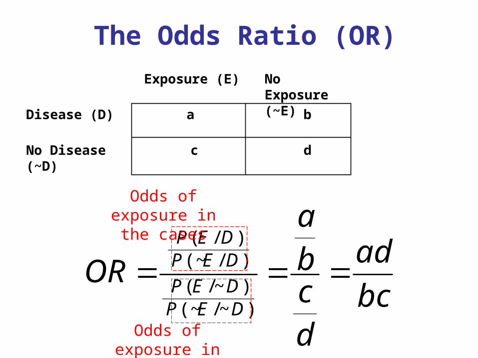
Exposure (E) No Exposure (~E)

Disease (D) a b

No Disease (~D) c d

The Odds Ratio (OR)

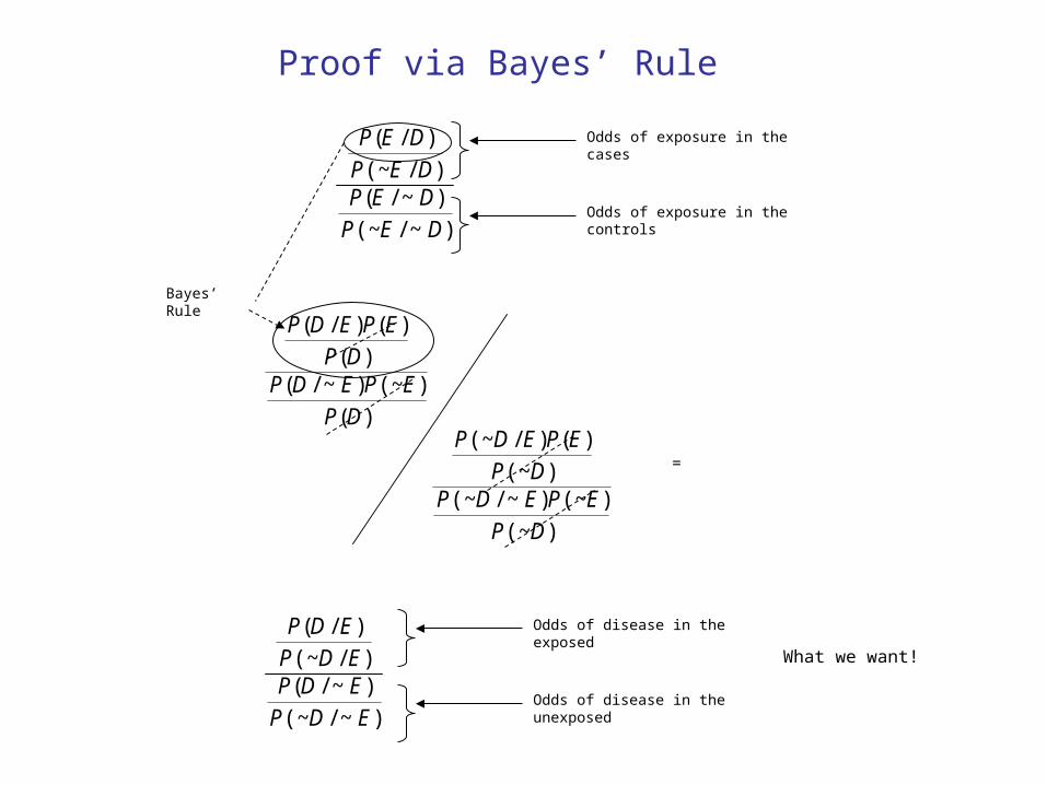
Odds of exposure in the cases

Odds of exposure in the controls

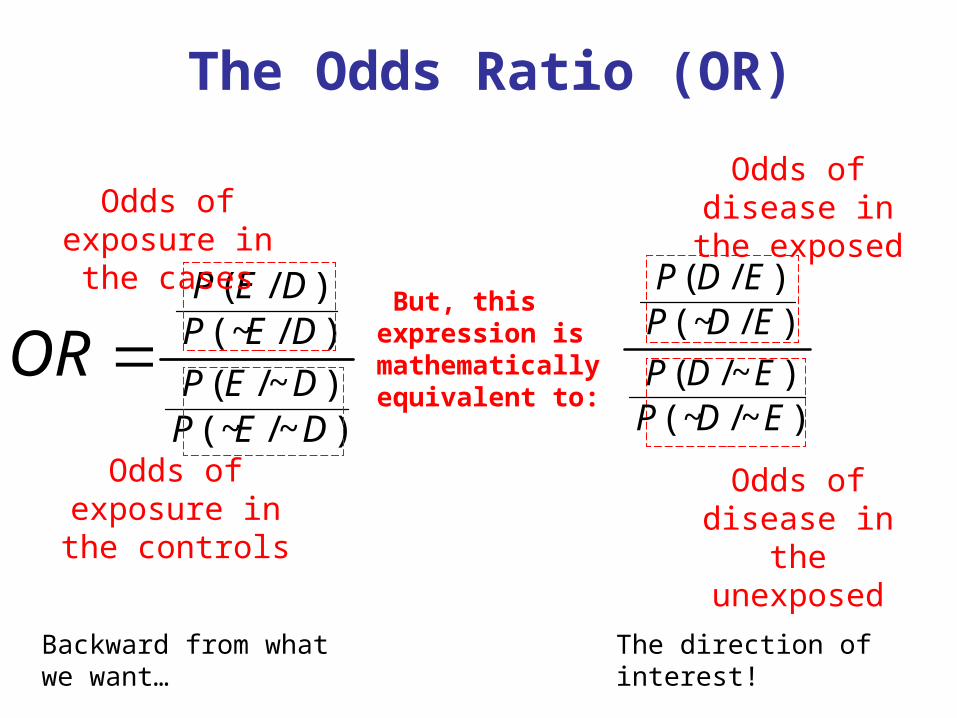
The Odds Ratio (OR)

Odds of disease in the exposed

Odds of disease in the unexposed

)~/(~)~/(

)/(~)/(

DEPDEP

DEPDEP

OR



)~/(~)~/(

)/(~)/(

EDPEDP

EDPEDP

But, this expression is mathematically equivalent to:

Backward from what we want…

The direction of interest!

=



Bayes’ Rule

Odds of disease in the unexposed

Odds of disease in the exposed

What we want!

)~/(~

)~/()/(~

)/(

DEP

DEPDEP

DEP

)(~

)(~)~/(~)(~

)()/(~)(

)(~)~/()(

)()/(

DP

EPEDPDP

EPEDPDP

EPEDPDP

EPEDP

)~/(~

)~/()/(~

)/(

EDP

EDPEDP

EDP

Proof via Bayes’ Rule

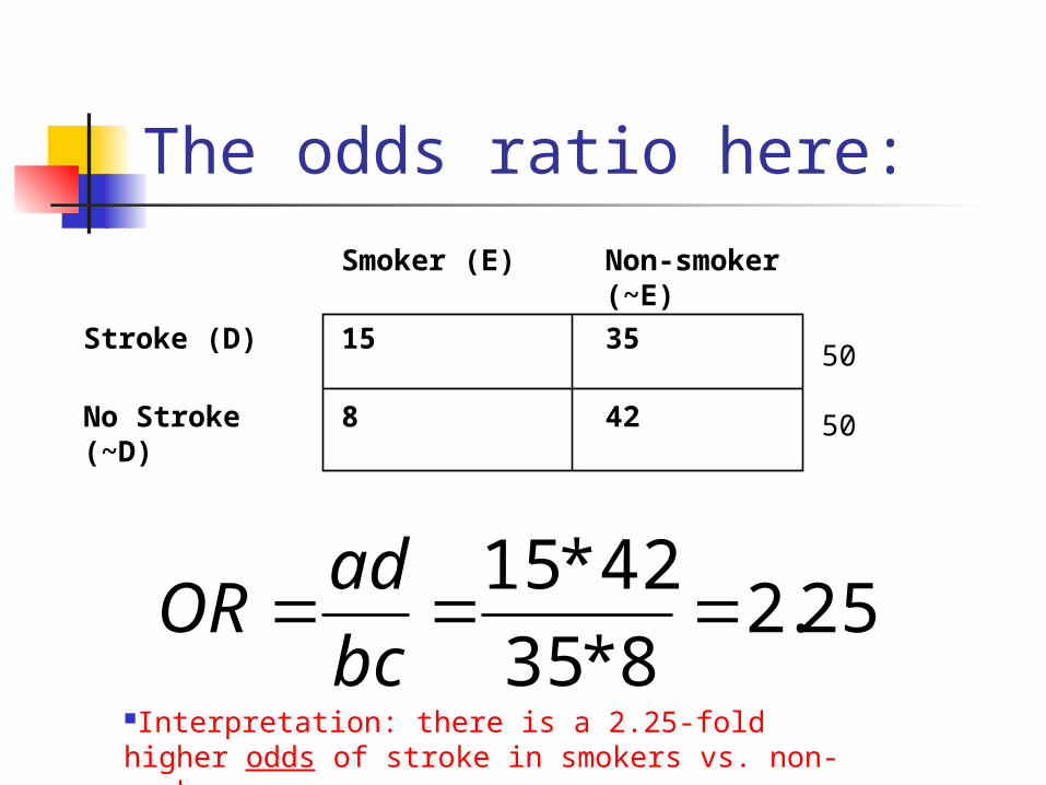
The odds ratio here:


Stroke (D) 15 35

No Stroke (~D) 8 42

50

50

25.28*35

42*15

bc

adOR

Interpretation: there is a 2.25-fold higher odds of stroke in smokers vs. non-smokers.

Interpretation of the odds ratio:

The odds ratio will always be bigger than the corresponding risk ratio if RR >1 and smaller if RR <1 (the harmful or protective effect always appears larger)

The magnitude of the inflation depends on the prevalence of the disease.

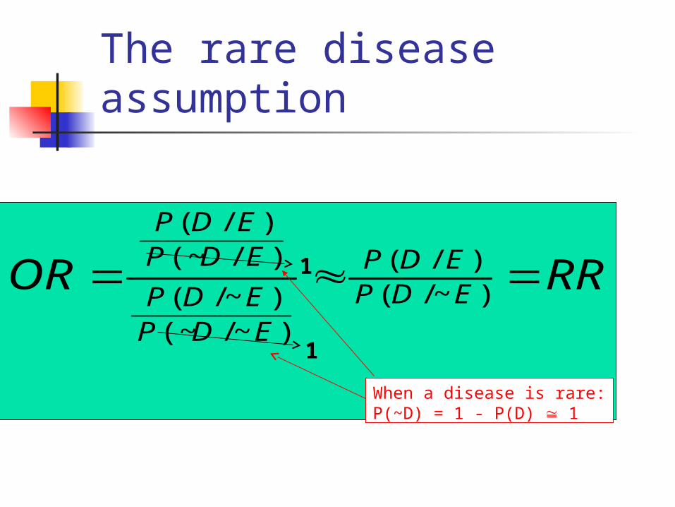
The rare disease assumption

RROR EDPEDP

EDPEDP

EDPEDP

)~/()/(

)~/(~)~/(

)/(~)/(

1

1

When a disease is rare: P(~D) = 1 - P(D) 1

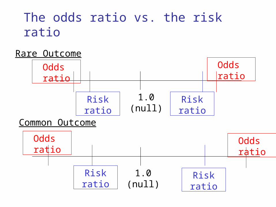
The odds ratio vs. the risk ratio

1.0 (null)

Odds ratio

Risk ratio Risk ratio

Odds ratio

Odds ratio

Risk ratio Risk ratio

Odds ratio

Rare Outcome

Common Outcome

1.0 (null)

Odds ratios in cross-sectional and cohort studies… Many cohort and cross-sectional studies report

ORs rather than RRs even though the data necessary to calculate RRs are available. Why?

If you have a binary outcome and want to adjust for confounders, you have to use logistic regression.

Logistic regression gives adjusted odds ratios, not risk ratios (more on this in HRP 261).

These odds ratios must be interpreted cautiously (as increased odds, not risk) when the outcome is common.

When the outcome is common, authors should also report unadjusted risk ratios and/or use a simple formula to convert adjusted odds ratios back to adjusted risk ratios.

Example, wrinkle study… A cross-sectional study on risk factors for

wrinkles found that heavy smoking significantly increases the risk of prominent wrinkles. Adjusted OR=3.92 (heavy smokers vs.

nonsmokers) calculated from logistic regression.

Interpretation: heavy smoking increases risk of prominent wrinkles nearly 4-fold??

The prevalence of prominent wrinkles in non-smokers is roughly 45%. So, it’s not possible to have a 4-fold increase in risk (=180%)!

Raduan et al. J Eur Acad Dermatol Venereol. 2008 Jul 3.

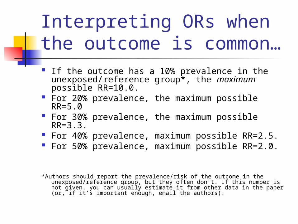
Interpreting ORs when the outcome is common… If the outcome has a 10% prevalence in the

unexposed/reference group*, the maximum possible RR=10.0.

For 20% prevalence, the maximum possible RR=5.0

For 30% prevalence, the maximum possible RR=3.3.

For 40% prevalence, maximum possible RR=2.5. For 50% prevalence, maximum possible RR=2.0.

*Authors should report the prevalence/risk of the outcome in the unexposed/reference group, but they often don’t. If this number is not given, you can usually estimate it from other data in the paper (or, if it’s important enough, email the authors).

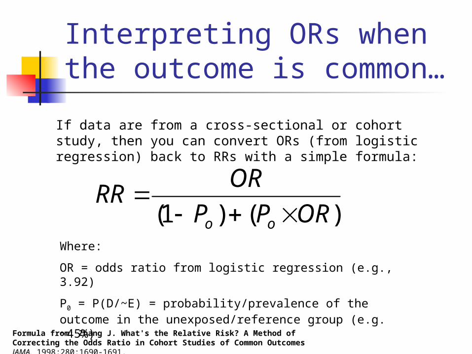
Interpreting ORs when the outcome is common…

Formula from: Zhang J. What's the Relative Risk? A Method of Correcting the Odds Ratio in Cohort Studies of Common Outcomes JAMA. 1998;280:1690-1691.

)()1( ORPP

ORRR

oo

Where:

OR = odds ratio from logistic regression (e.g., 3.92)

P0 = P(D/~E) = probability/prevalence of the outcome in the unexposed/reference group (e.g. ~45%)

If data are from a cross-sectional or cohort study, then you can convert ORs (from logistic regression) back to RRs with a simple formula:

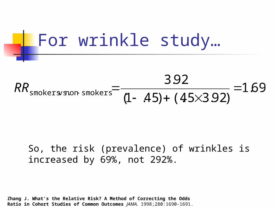
For wrinkle study…

Zhang J. What's the Relative Risk? A Method of Correcting the Odds Ratio in Cohort Studies of Common Outcomes JAMA. 1998;280:1690-1691.

69.1)92.345(.)45.1(

92.3smokersnon vs.smokers

RR

So, the risk (prevalence) of wrinkles is increased by 69%, not 292%.

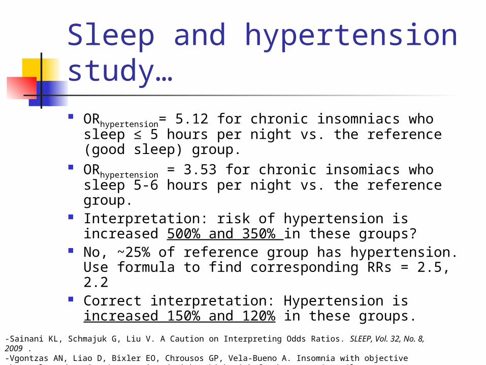
Sleep and hypertension study… ORhypertension= 5.12 for chronic insomniacs who

sleep ≤ 5 hours per night vs. the reference (good sleep) group.

ORhypertension = 3.53 for chronic insomiacs who sleep 5-6 hours per night vs. the reference group.

Interpretation: risk of hypertension is increased 500% and 350% in these groups?

No, ~25% of reference group has hypertension. Use formula to find corresponding RRs = 2.5, 2.2

Correct interpretation: Hypertension is increased 150% and 120% in these groups.

-Sainani KL, Schmajuk G, Liu V. A Caution on Interpreting Odds Ratios. SLEEP, Vol. 32, No. 8, 2009 .-Vgontzas AN, Liao D, Bixler EO, Chrousos GP, Vela-Bueno A. Insomnia with objective short sleep duration is associated with a high risk for hypertension. Sleep 2009;32:491-7.

Practice problem:

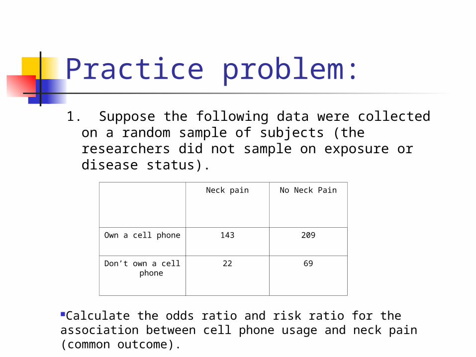
1. Suppose the following data were collected on a random sample of subjects (the researchers did not sample on exposure or disease status).

Calculate the odds ratio and risk ratio for the association between cell phone usage and neck pain (common outcome).

Neck pain No Neck Pain

Own a cell phone 143 209

Don’t own a cell phone 22 69

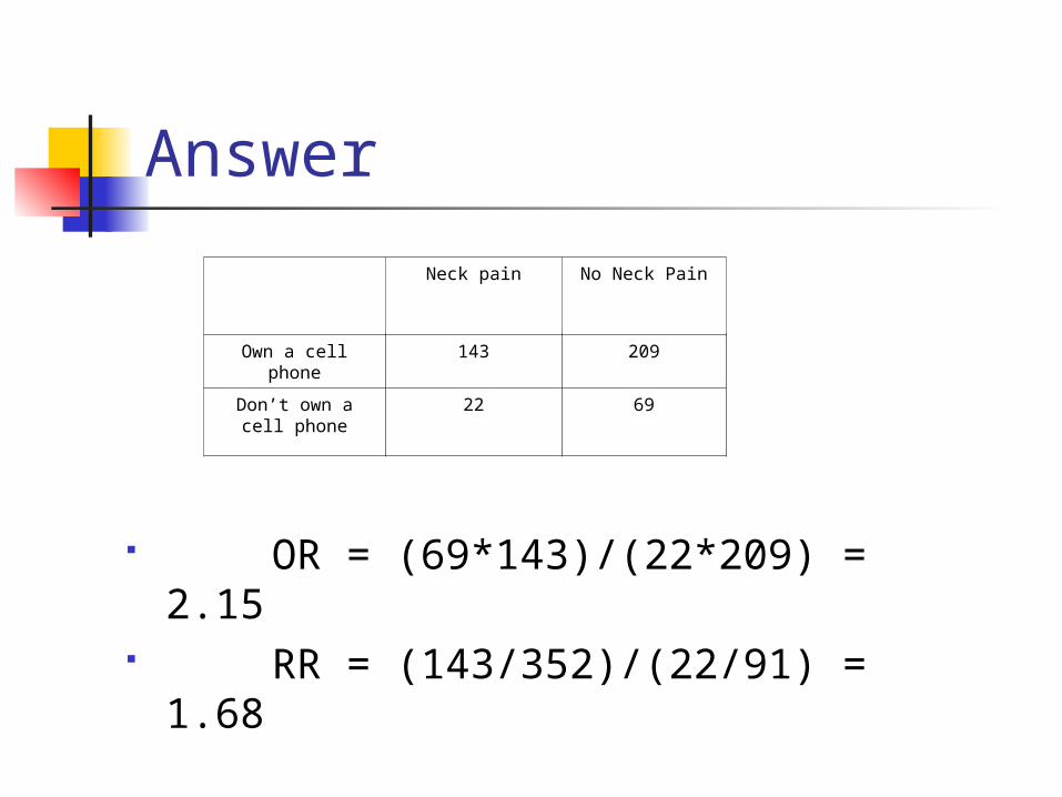
Answer

OR = (69*143)/(22*209) = 2.15 RR = (143/352)/(22/91) = 1.68

Neck pain No Neck Pain


Don’t own a cell phone

22 69

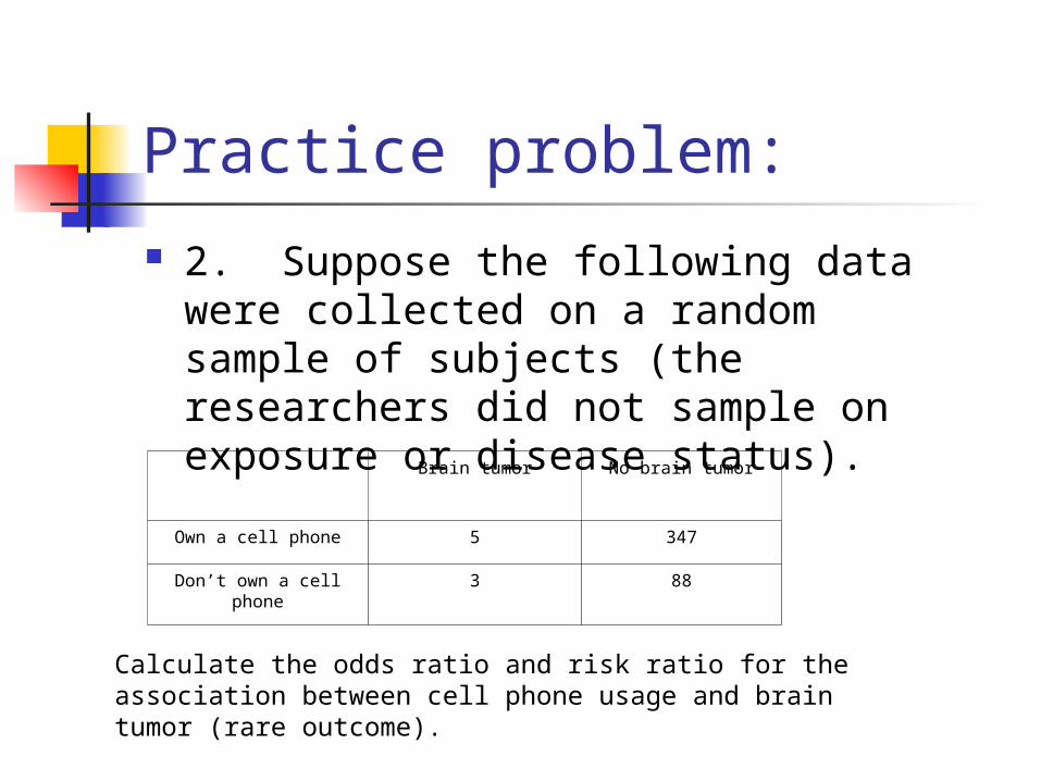
Practice problem: 2. Suppose the following data were

collected on a random sample of subjects (the researchers did not sample on exposure or disease status).

Calculate the odds ratio and risk ratio for the association between cell phone usage and brain tumor (rare outcome).

Brain tumor No brain tumor


Don’t own a cell phone 3 88

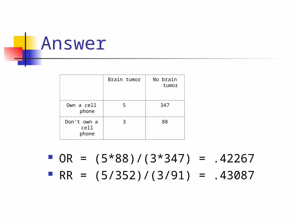
Answer

OR = (5*88)/(3*347) = .42267 RR = (5/352)/(3/91) = .43087

Brain tumor No brain tumor


Don’t own a cell phone

3 88

Thought problem… Another classic first-year statistics

problem. You are on the Monty Hall show. You are presented with 3 doors (A, B, C), only one of which has something valuable to you behind it (the others are bogus). You do not know what is behind any of the doors. You choose door A; Monty Hall opens door B and shows you that there is nothing behind it. Then he gives you the option of sticking with A or switching to C. Do you stay or switch? Does it matter?

Some Monty Hall links…

http://query.nytimes.com/gst/fullpage.html?res=9D0CEFDD1E3FF932A15754C0A967958260&sec=&spon=&pagewanted=all

http://www.nytimes.com/2008/04/08/science/08tier.html?_r=1&em&ex=1207972800&en=81bdecc33f60033e&ei=5087%0A&oref=slogin

http://www.nytimes.com/2008/04/08/science/08monty.html#

Documents

Conditional Probability And the odds ratio and risk ratio as conditional probability