A Class of Methods for Solving Nonlinear Simultaneous EquationsAuthor(s): C. G. BroydenSource: Mathematics of Computation, Vol. 19, No. 92 (Oct., 1965), pp. 577-593Published by: American Mathematical SocietyStable URL: http://www.jstor.org/stable/2003941Accessed: 16/11/2009 12:31

Your use of the JSTOR archive indicates your acceptance of JSTOR's Terms and Conditions of Use, available athttp://www.jstor.org/page/info/about/policies/terms.jsp. JSTOR's Terms and Conditions of Use provides, in part, that unlessyou have obtained prior permission, you may not download an entire issue of a journal or multiple copies of articles, and youmay use content in the JSTOR archive only for your personal, non-commercial use.

Please contact the publisher regarding any further use of this work. Publisher contact information may be obtained athttp://www.jstor.org/action/showPublisher?publisherCode=ams.

Each copy of any part of a JSTOR transmission must contain the same copyright notice that appears on the screen or printedpage of such transmission.

JSTOR is a not-for-profit service that helps scholars, researchers, and students discover, use, and build upon a wide range ofcontent in a trusted digital archive. We use information technology and tools to increase productivity and facilitate new formsof scholarship. For more information about JSTOR, please contact support@jstor.org.

American Mathematical Society is collaborating with JSTOR to digitize, preserve and extend access toMathematics of Computation.

http://www.jstor.org

A Class of Methods for Solving Nonlinear Simultaneous Equations

By C. G. Broyden

1. Introduction. The solution of a set of nonlinear simultaneous equations is often the final step in the solution of practical problems arising in physics and engi- neering. These equations can be expressed as the simultaneous zeroing of a set of functions, where the number of functions to be zeroed is equal to the number of independent variables. If the equations form a sufficiently good description of a physical or engineering system, they will have a solution that corresponds to some state of this system. Although it may be impossible to prove by mathematics alone that a solution exists, this fact may be inferred from the physical analogy. Similarly, although the solution may not be unique, it is hoped that familiarity with the physi- cal analogue will enable a sufficiently good initial estimate to be found so that any iterative process that may be used will in fact converge to the physically significant solution.

The functions that require zeroing are real functions of real variables and it will be assumed that they are continuous and differentiable with respect to these varia- bles. In many practical examples they are extremely complicated anld hence la- borious to compute, an-d this fact has two important immediate consequences. The first is that it is impracticable to compute any derivative that may be required by the evaluation of the algebraic expression of this derivative. If derivatives are needed they must be obtained by differencing. The second is that during any iterative solution process the bulk of the computing time will be spent in evaluating the functions. Thus, the most efficient process will tenid to be that which requires the smallest number of function evaluations.

This paper discusses certain modificatioins to Newton's method designed to re- duce the number of function evaluations required. Results of various numerical experiments are given and conditions under which the modified versions are superior to the original are tentatively suggested.

2. Newton's Method. Consider the set of n nonlinear equations

(2.1) (x, , 2 , x) = 0, j = 1, 2, .., n.

These may be written more concisely as

(2.2) f(x) = 0

where x is the column vector of independent variables and f the column vector of functions fj . If xi is the ith approxinmation to the solution of (2.2) and fi is written for f(xi), then Newton's m-ethod (see e.g. [4]) is defined by

(2.3) x+, = xi- Ai

where Ai is the Jacobian matrix [afj&vXk] evaluated at xi. Now Newton's miethod, as expressed in equation (2.3), suffers from two serious

Received April 20, 1965.

577

578 C. G. BROYDEN

disadvantages from the point of view of practical calculation. The first of these is the difficulty of computing the Jacobian matrix. Even if the functions fj are suf- ficiently simple for their partial derivatives to be obtained analytically, the anmount of labour required to evaluate all n2 of these may well be excessive. In the majority of practical problems, however, the fj's are far too conmplicated for this, and an approxinmation to the Jacobian nmatrix must be obtained numerically. This is often carred out directly, i.e., afj/axk is computed by evaluating fj for two different values of Xk while holding the remaining n - 1 independent variables constant. Although this direct approach gives an immediate approximation to the partial derivatives, it is not without its disadvantages, the nmost serious of which is the amount of labour involved. For in order to compute the Jacobian matrix in this way the vector func- tion f nmust be evaluated for at least n + 1 sets of independent variables.

The second disadvantage of Newton's method is the fact that without some mod- ifications it frequently fails to converge. Conditions for convergence are in fact well known (see e.g. [4]), but they rely on the initial estimate of the solution being sufficiently good, a requirement that is often inmpossible to realise in practice. Hence Newton's method, as defined by (2.3), cannot be regarded as a good practical algorithm.

Despite these disadvantages, however, the method has much to commend it. The algorithm is simple, even though it does require the solution of n linear equa- tions at every step, it has a sound theoretical basis and for many problenms its convergence is rapid. Furthermore, it has few competitors. The methods based upon mniniimising some norm of the vector f by the steepest descent or some similar method tend to converge slowly if the problemn is at all ill-conditioned, although the very new nmethod described by Kizner [5] nmay ultimately prove to be nmore satisfactory.

In order to overcome some of the disadvantages of Newton's method it has been suggested that the Jacobian nmatrix be evaluated either once and for all or once every few iterations, instead of at every iteration as is strictly required. Both these variants, however, require the complete evaluation of the Jacobian matrix. In the class of methods described in this paper the partial derivatives afj/lXk are not estimated or evaluated directly, but corrections to the approximate inverse of the Jacobian matrix are computed from values of the vector function f.

A correction of this type is carried out at each iteration and is nmuch simpler to perforin than the evaluation of the complete Jacobian. It is hoped, therefore, that this class of methods conmbines to some extent the simplicity of the constant matrix (once for all) method with the ultimatelv rapid convergence of the basic Newton method.

3. The Class of Methods. Let xi be the ith approximation to the solution of (2.2) and defined pi by

(3.1) pi = -Bi-fi

where Bi is somiie approximation to the Jacobian mnatrix evaluated at xi. Then a simple modification to Newton's algorithm gives xi+1 by

(3.2) xi+1 = xi + tips,

where li, whose derivation will be discussed in section 5, is a scalar multiplier chosen

SOLVING NONLINEAR SIMULTANEOUS EQUATIONS 579

to prevent the process diverging. Let x now be defined as

(3.3) xxi + tpi,

where t may take any arbitrary value. The functions fj may now be regarded as functions of the single variable t and, since the partial derivatives Ofj/t3Xk are as- sumed to exist, possess a first derivative with respect to t. It will now be shown that an approximation to the derivatives dfj/dt, j = 1, 2, , n, may be used to improve the approximate Jacobian matrix B13 .

Since x is now assumed to be a function of t alone,

dfj _ E dX k d~th k-lOxk dt

and if by df/dt is understood the vector [dfj/dt], equation (3.4) becomes

(3.5) d= Ap where A is the Jacobian matrix. Hence if an accurate estimate of df/dt were avail- able, it could be used, via equation (3.5), to establish a condition that any approxi- mation to the Jacobian matrix must satisfy. Now it has already been assumed that the functions fi are sufficiently complicated for analytic expressions of their first partial derivatives not to be available; the only way of obtaining an estimate to df/dt is by differencing. Since the aim is to obtain an approximation to the Jacobian matrix at the point xi+,, it is necessary to obtain an approximation to df/dt at this point. Hence expand each fj, still regarded as a function of t alone, as a Taylor series about ti and assunme that the second and higher-order terms are small, giving

(3.6) f(ti - s) -fd -s df

Hence when fi+? and f(ti - si), where si is a particular value of s whose choice will be discussed in section 6, have been computed, equation (3.6) may be used without the need for further evaluations of the function f to obtain an approxima- tion of df/dt and hence to inmpose a condition upon any approxinmation to the Jacobian matrix. No special evaluation of f is ever necessary to do this since if s is put equal to ti, f(ti - s) becomes fi, a known quantity. Eliminating df/dt between (3.5) and (3.6) then gives

(3.7) f -+1 f (tI - si) siApi .

Consider now equation (3.7). It relates four quantities that have already been computed to a fifth, the Jacobian matrix A, to which only an approximation Bi is available and to which a better approximation B2+1 is sought. Now in the class of nmethods discussed in this paper Bj+1 is chosen in such a way as to satisfy the equation

(3.8) f +1 - f(ti - si) = sjBj+jp.

On comparing equations (3.7) and (3.8) it is seen that if the error in (3.7) is negligible, i.e., if the suin of the second and higher-order terms in the Taylor series expansion of each f, is sufficiently small, then Bj+1 will have at least one of the re-

580 C. G. BROYDEN

quired properties of the Jacobian matrix. If, on the other hand, the omitted sums are large, the matrix Bj+1 will not approximate to the Jacobian matrix. Hence it would appear reasonable to choose si to be as small as possible consistent with not introducing excessive rounding error into the estimate of df/dt.

If si is put equal to ti, equation (3.8) becomes

(3.9) f+- fi=tiB+1pi;

and this shows that the jth element of the vector Bi+lpi assunmes, from the first Mean Value Theorem, the value of dfj/dt evaluated at some point, which varies with j, between xi anad xi+,. Although this is not as good as obtaining a set of derivatives evaluated at xi+,, it does ensqre that Bj+1 refers to points closer to the solution than xi, since xi+, is, in some sense, a better approximation to the solution than xi.

Now if the calculation is carried out holding the matrix Bi in the store of the computer, it will be necessary to solve n linear equations to compute, using equa- tion (3.1), the step direction vector pi ; but if the inverse of this matrix is stored, this operation is reduced to a matrix-vector multiplication. If Hi and yi are defined by

(3.10) Hi= -Bi

and

(3.11) Yi = fi1 - f(ti -S

equations (3.1) and (3.8) become

(3.12) pi-Hif

and

(3.13) H =1y- STpi

Equation (3.13) does not, like equation (3.8), define a unique matrix but a class of matrices. Hence equations (3.2) and (3.11 )-(3.13) define a class of methods based upon that of Newton for solving a set of nonlinear simultaneous equations, and these methods will subsequently be referred to as quasi-Newton methods. By making further assumptions about the properties of Bi+, or Hi+, particular methods may be derived.

The most important feature of the quasi-Newton methods is that although the iteration matrix Hi changes from step to step, no evaluations of f(x) are required beyond those that would be necessary if Hi remained constant. This is an important consideration if the vector function f is laborious to compute. Another feature of these methods is that as xi approaches the solution the assumptions nmade in deriving (3.6) become more valid. Hence if Bi tends to the Jacobian matrix, the rate of convergence may be expected to improve as the solution is approached, becoming ultimately quadratic.

4. Particular Methods. Method 1. In the previous section a class of methods was derived in which the

new approximation Bi,1 to the Jacobian matrix is required to satisfy an equation

SOLVING NONLINEAR SIMULTANEOUS EQUATIONS 581

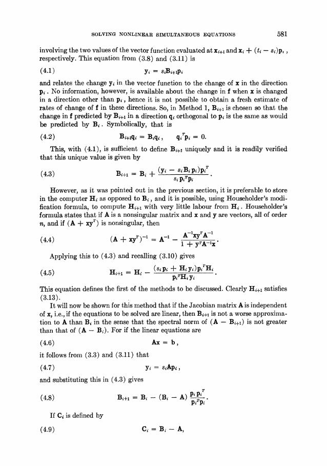
involving the two values of the vector function evaluated at xi+, and xi + (ti -s0p, respectively. This equation from (3.8) and (3.11) is

(4.1) yi = sjBj+jpi

and relates the change yi in the vector function to the change of x in the direction pi. No information, however, is available about the change in f when x is changed in a direction other than pi, hence it is not possible to obtain a fresh estimate of rates of change of f in these directions. So, in Method 1, Bj+j is chosen so that the change in f predicted by Bi+1 in a direction qi orthogonal to pi is the same as would be predicted by Bi. Symbolically, that is

(4.2) B+lqi= Biq, qiTpi = 0.

This, with (4.1), is sufficient to define Bj+1 uniquely and it is readily verified that this unique value is given by

(4.3) Bi+j = Bi + (yi- siBpi)piT

However, as it was pointed out in the previous section, it is preferable to store in the computer Hi as opposed to Bi, and it is possible, using Householder's modi- fication formula, to compute Hi+1 with very little labour from Hi. Householder's formula states that if A is a nonsingular matrix and x and y are vectors, all of order n, and if (A + XyT) is nonsingular, then

(4.4) (A + xy7) = -1 _ A y TA'

Applying this to (4.3) and recalling (3.10) gives

(4.5) Hi+, = Hi - (sipi + Hiyi)pT Hi

This equation defines the first of the methods to be discussed. Clearly Hi+1 satisfies (3.13).

It will now be shown for this method that if the Jacobian matrix A is independent of x, i.e., if the equations to be solved are linear, then Bi+j is not a worse approxima- tion to A than Bi in the sense that the spectral norm of (A - Bi+1) is not greater than that of (A - Bi). For if the linear equations are

(4.6) Ax= b,

it follows from (3.3) and (3.11) that

(4.7) yi= siApi,

and substituting this in (4.3) gives

(4.8) B+= - (B - A) pi PiT

If Ci is defined by

(4.9) C= Bi - A,

582 C. G. BROYDEN

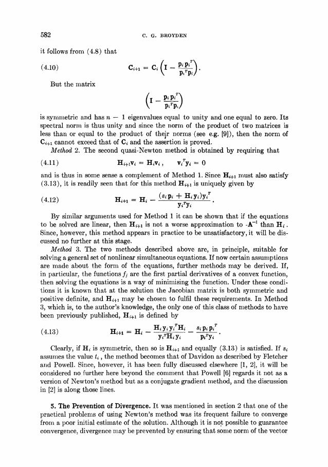
it follows from (4.8) that

(4.10) C+1 (I _p_Tp)

But the matrix

Pi pi pTA

is symmetric and has n - 1 eigenvalues equal to unity and one equal to zero. Its spectral norm is thus unity and since the norm of the product of two matrices is less than or equal to the product of their norms (see e.g. [9]), then the norm of Ci+1 cannot exceed that of Ci and the assertion is proved.

Method 2. The second quasi-Newton method is obtained by requiring that

(4.11) Hi+lvi = Hivi, ViTyi= 0

and is thus in some sense a complement of Method 1. Since Hi+1 must also satisfy (3.13), it is readily seen that for this method Hi+ is uniquely given by

(4.12) Hi+1 - Hi - + yi)y

By similar arguments used for Method 1 it can be shown that if the equations to be solved are linear, then Hi+, is not a worse approximation to -A-' than Hi. Since, however, this method appears in practice to be unsatisfactory, it will be dis- cussed no further at this stage.

Method 3. The two methods described above are, in principle, suitable for solving a general set of nonlinear simultaneous equations. If now certain assumptions are made about the form of the equations, further methods may be derived. If, in particular, the functions fj are the first partial derivatives of a convex function, then solving the equations is a way of minimising the function. Under these condi- tions it is known that at the solution the Jacobian matrix is both symmetric and positive definite, and Hi+, may be chosen to fulfil these requirements. In Method 3, which is, to the author's knowledge, the only one of this class of methods to have been previously published, Hi+, is defined by

(4.13) Hi+, = Hi- y Hi yH _ - yips

Clearly, if Hi is symmetric, then so is Hi+, and equally (3.13) is satisfied. If Si

assumes the value t,, the method becomes that of Davidon as described by Fletcher and Powell. Since, however, it has been fully discussed elsewhere [1, 2], it will be considered no further here beyond the comment that Powell [6] regards it not as a version of Newton's method but as a conjugate gradient method, and the discussion in [2] is along those lines.

5. The Prevention of Divergence. It was mentioned in section 2 that one of the practical problems of using Newton's method was its frequent failure to converge from a poor initial estimate of the solution. Although it is not possible to guarantee convergence, divergence may be prevented by ensuring that some norm of the vector

SOLVING NONLINEAR SIMULTANEOUS EQUATIONS 583

function fi is a nonincreasing function of i. The simplest, and that used in the author's program, is the Euclidean norm although of course others may be employed.

In the practical application of one of the methods described in section 4, once a step direction pi has been obtained from equation (3.12), x is constrained to satisfy equation (3.3) so that, until xi+, has been determined, f(x) and its norm become functions of t alone. The value ti of t that is finally used to determine xi+, may then be chosen in various ways, and two of these are now considered.

In the first method ti is chosen to minimise the norm of f +1 . This is, perhaps, the most obvious choice to make since it gives the greatest immediate reduction of the norm and hence, in some sense, the greatest improvement to the approximate solu- tion. However, in order to do this the vector function f needs to be eva4uated a number of times, and this means an increase in the amount of compu- tation required compared with the alternative strategy of choosing a value of ti which merely reduces the norm. Frequently the original Newtonian value of unity is sufficient to do this, but even if it is not, it will be less laborious to reduce the norm than to minimise it. Reducing the norm does not, of course, give as good an immediate improvement to the solution as norm minimisation, but it does mean that less work is involved in correcting the matrix Hi.

The relative merits of these opposing strategies, that of obtaining the greatest improvement to the solution during one step or that of using the new information as soon as possible to correct Hi and compute a new xi+,, are difficult to assess from theory alone and recourse must be made to numerical experiment. The results of applying these two strategies to various problems are discussed in sections 9 and 10.

6. The Choice of s8i. Since Bi is required to approximate as closely as possible to the Jacobian matrix, it is reasonable to choose si so that df/dt is approximated as closely as possible, and this implies that si should be as small as possible consistent with the difference between f(ti - s8) and f(ti) being large enough for rounding error to be unimportant. However, it is also desirable for there to be no further evaluations of the vector function f, use being made only of those values of the func- tion computed in the course of minimising or reducing the norm. If the strategy of norm reduction is adopted and if the first value of t chosen results in the norm being reduced, then ti is taken to be this value, and the only possible value that si can assume without extra function evaluation is ti. If, however, more than one evalua- tion is needed to reduce the norm or if the norm minimisation method is used, then there is a certain amount of latitude about the choice of si within the requirement that no further evaluations are permitted. It may still be chosen to be ti but from the point of view of minimising truncation error the smallest possible s should be chosen. This, however, is not easy to implement in practice. For assume that the norm N(t) has been evaluated successively at t = t(k), k = 1, 2, ... , m, where

(6.1) t= 1,

(6.2) t(m) =ti,

and where ti is either the value of t that minimises N or the first t(k) for which N(t(k)) < N(0). If s(k) is defined by

584 c. G. BROYDEN

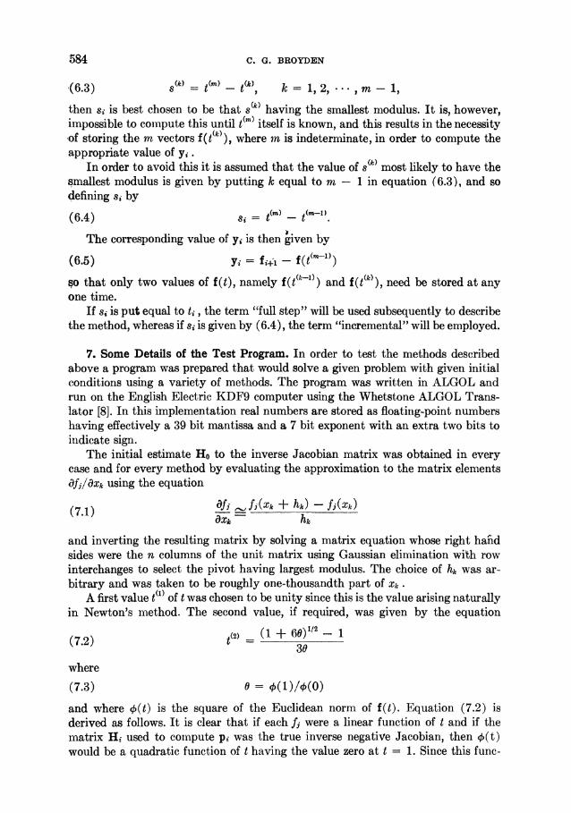
(6.3) s() =t" t(k) k 1,2, , m- 1,

then si is best chosen to be that 8(k) having the smallest modulus. It is, however, impossible to compute this until t(m) itself is known, and this results in the necessity of storing the mn vectors f(t(k)), where in is indeterminate, in order to compute the appropriate value of yi.

In order to avoid this it is assumed that the value of s most likely to have the smallest modulus is given by putting k equal to m - 1 in equation (6.3), and so defining si by

(6.4) s=t(m) -t'r-l)

The corresponding value of yi is then given by

(6.5) yi = fi.l - f(t (1))

so that only two values of f(t), namely f(t(k-1)) and f(t(k)), need be stored at any one time.

If si is put equal to t,, the term "full step" will be used subsequently to describe the method, whereas if si is given by (6.4), the term "incremental" will be employed.

7. Some Details of the Test Program. In order to test the methods described above a program was prepared that would solve a given problem with given initial conditions using a variety of methods. The program was written in ALGOL and run on the English Electric KDF9 computer using the Whetstone ALGOL Trans- lator [8]. In this implementation real numbers are stored as floating-point numbers having effectively a 39 bit mantissa and a 7 bit exponent with an extra two bits to indicate sign.

The initial estimate Ho to the inverse Jacobian matrix was obtained in every case and for every method by evaluating the approximation to the matrix elements af /oxa using the equation

(7.1) 'Ofj fj,f(xk + hk) - fJ(Xk) OXk hk

and inverting the resulting matrix by solving a matrix equation whose right hand sides were the n columns of the unit matrix using Gaussian elimination with row interchanges to select the pivot having largest modulus. The choice of hk was ar- bitrary and was taken to be roughly one-thousandth part of xk .

A first value t(') of t was chosen to be unity since this is the value arising naturally in Newton's method. The second value, if required, was given by the equation

(7.2) t(2) (1 + 60)1/2 - 1 (7.2) t

~~~~~~~30

where

(7.3) 0 = 0(1)/0(0)

and where ?(t) is the square of the Euclidean norm of f(t). Equation (7.2) is derived as follows. It is clear that if each fj were a linear function of t and if the matrix Hi used to comnpute pi was the true inverse negative Jacobian, then +(t) would be a quadratic function of t having the value zero at t = 1. Since this func-

SOLVING NONLINEAR SIMULTANEOUS EQUATIONS 585.

tion cannot be negative, it must therefore have zero slope at t = 1. Denoting this ideal quadratic approximation by 4q(t), it follows that for pq(t) to satisfy the conditions at t = 1 it must be given by

(7.4) 4s(t) (1 - 2t + t2)0(0).

In practice, of course, the square of the Euclidean norm at t = 1 is very rarely equal to zero and the assumption is now made that this is due solely to the presence of an additional cubic term. Hence the function c is assumed to be approximated by the cubic function 45 where

(7.5) 4Cc 4q + at .

By putting t = 1 in (7.5) it follows that a = c(1) and hence

(7.6) Oc (1 - 2t + t2)c(O) + t3(1).

Now t(2) is chosen to be the value of t that minimises oc and differentiating (7.6), equating to zero and selecting the root lying between zero and unity gives equation (7.2).

If further improvement to 4 is required, it is approximated by a quadratic func- tion whose ordinates are specified at t = 0, 1 and t(2). If this function is convex, then t(3) is chosen to be the value of t that minimises it, and a new quadratic is formed whose ordinates are specified at t(3) and two of the previous triad of values of t. Since the precise method of reducing or mninimising the norm is peripheral to the theory, it will be described no further here, the actual ALGOL procedure used being given in Appendix 2.

The program, in addition to being able to test Methods 1 and 2 for any combina- tion of minirnising/reducing norm with incremental/full step choice of s was also able to test both the "constant matrix" and "basic" methods, either minimising or reducing the norm at each step. In the constant matrix method Ho is set up and inverted as described above, and this matrix is then used unchanged to obtain pi throughout the remainder of the calculation. In the basic method the matrix Hi is computed afresh at each step using the same algorithm that was employed to compute Ho. In the test program the increments hk were chosen initially to be about one-thousandth part of the variables xk and were then held constant for the rest of the calculation.

8. Basis for Comparison. The criteria by which the merit of any algorithm may be assessed are the accuracy of the solution obtained, the time taken to reach this solution and the amount of computer storage space used in the computation. Fre- quently the second of these criteria is in conflict with the first and the third and some arbitrary assumptions must be made before it is possible to give an overall comparison of two different algorithms.

In the comparisons made in this paper storage space requirements are omitted completely, time and accuracy alone being considered. Since it is impossible to com- pare times accurately when two methods are tested on two different machines or using two different programming systems, the further assumptions are made that the total amount of computation, and hence the time taken, is directly proportional to the number of evaluations of the vector function f that are necessary to obtain

586 C. G. BROYDEN

the solution and that the constant of proportionality is the same for all methods. This is approximately true when the functions are simple and becomes more nearly true as the complexity of the functions increases and the constant of proportionality approaches unity. This measure of computing time is clearly more satisfactory than the number of iterations since the amount of labour involved in an iteration may vary from the evaluation of n + 1 functions and the inversion of a matrix in the basic method to the evaluation of perhaps only one function and a few matrix- vector multiplications in Method 1 with norm reduction.

In order to compare the perforinance of the various methods under as nearly identical conditions as possible they were used to solve a set of test problems, starting each problem from the same initial conditions. Since, however, the course of computation varied with each method, it was impossible to terminate the calcu- lations at the same point; the accuracy of the final solution as measured by the Euclidean norm of the vector f varied froim method to method, although in each case the iteration was terminated as soon as this norm became less than a tolerance arbitrarily chosen to be 10-6. Now one of the characteristics of Newton's method is that the rate of convergence increases as the solution is approached and it is quite possible for the final iteration to reduce the norm of f by as much as a factor of 10-2.

Hence although the iteration is terminated immediately the norm becomes less than 10-6, the final norm may be as low as 10-8, and it was thought necessary to include this variation when assessing the merit of a particular method.

The measure of efficiency of a method for solving a particular problem was thus chosen to be the mean convergence rate R, where R is given by

(8.1) R= lIn L m Nms

and where m is the total number of function evaluations and N1, Nm the initial and final Euclidean norms of f.

Although this definition of R is similar to Varga's definition of mean convergence rate [10], it must be emphasised that the R defined by (8.1) has none of the properties of that defined by Varga and in particular does not tend to an asymptotic value as n -- oo. It is merely intended to be a concise index of the performance of a method

applied to a particular problem in a particular situation and has no relevance outside the context of the problem and situation to which it refers.

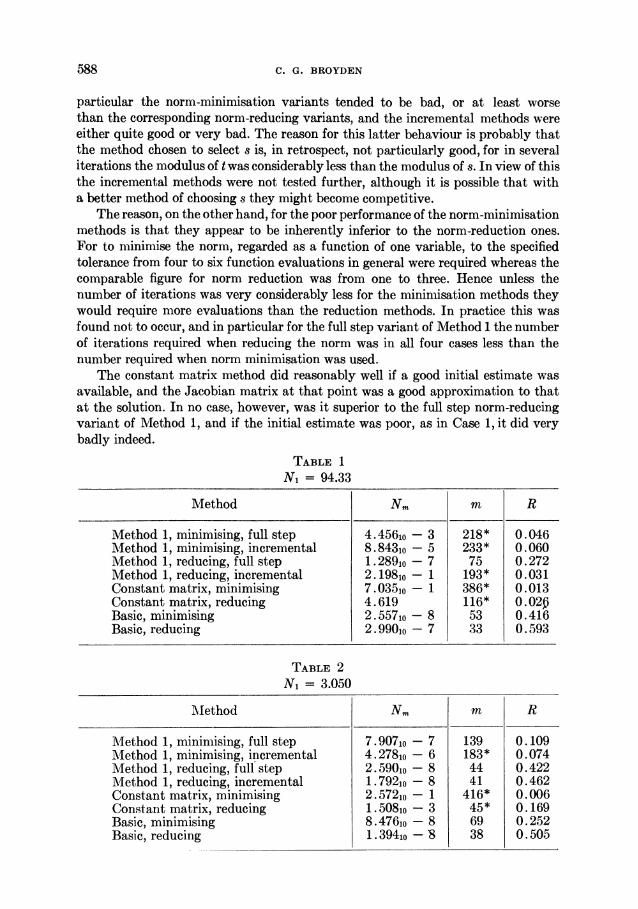
9. Case Histories and Discussion. This section is devoted to a discussion of the behaviour of the various methods when applied to a number of test cases. The per- formance of the methods are summarised for each test problem in a table which gives the initial and final Euclidean norms N1 and Nm of f, the total number m of function evaluations required to reduce the norm to Nm and the mean rate of con- vergence R as defined in the previous section. The number of function evaluations m includes in every case those evaluations required initially to set up the approxi- mation to the Jacobian matrix, and an asterisk against this figure indicates that the iteration had not converged after that number of evaluations, and the run had been terminated since the number of evaluations already exceeded the nunlber needed for convergence using a superior method. The tables are numbered to correspond with the case numbers.

SOLVING NONLINEAR SIMULTANEOUS EQUATION 587

While the program was being developed, it became increasingly apparent that Method 2 was quite useless. In every case tried it rapidly reached a state where suc- cessive step vectors pi and pi+, were identical and further progress thus became im- possible, and for this reason it is omitted from the following case histories.

Cases 1-3. The equations from these three cases arose from design studies on a pneumatically-damped hydraulic system and involve both logarithms and fractional powers. The three cases analysed were taken from a large number of cases, all of which were difficult to solve. The first case has three independent variables and the second and third four. The third case is merely the second case with an improved initial estimate.

Case 4. The equations here represent a counterflow gas/water steam-raising unit. They involve logarithms and various polynomial approximations of physical quantities, e.g. the saturation temperature of water as a function of pressure. There are only two independent variables and despite the magnitude of N1 the equations were much easier to solve than those used to provide Cases 1-3.

Cases 5-8. These cases solved the specially-constructed equations:

fi = -(3 + aXO)XI + 2x2 -,

fi = Xi-,l-(3 + aexi)xi + 2xj+I -X i = 2, 3, n *, n 1,

fn = x.-1 - (3 + ax.) x - f3.

Values of a, A and n are given in the tables, and the initial estimates in all cases were

X -1.0, i = 1, 2, n.., n.

Case 9. These equations were taken from a paper by Powell [7]:

fl = 1O(x2 -Xi )

,f2 = 1 -x,

and the initial values of the independent variables were

x= -1.2,

x2= 1.0.

Case 10. The equations for this case were due to Freudenstein and Roth [3]:

fi = -13 + xi +((-x2 + 5)x2-2)x2,

f2 = -29 + xi + ((X2 + 1)x2 - 14)x2.

The initial values were

xl = 15,

X2 = -2.

An examination of Tables 1-4 shows that of the eight methods tested, three were consistently good for all the first four test cases. These were the full step norlm-re- ducing variant of Method 1 and both versions of the basic method. All the other methods were either uniformly bad, or tended to be erratic in their behaviour. In

588 C. G. BROYDEN

particular the norm-minimisation variants tended to be bad, or at least worse than the corresponding norm-reducing variants, and the incremental methods were either quite good or very bad. The reason for this latter behaviour is probably that the method chosen to select s is, in retrospect, not particularly good, for in several iterations the modulus of t was considerably less than the modulus of s. In view of this the incremental methods were not tested further, although it is possible that with a better method of choosing s they might become competitive.

The reason, on the other hand, for the poor performance of the norm-minimisation methods is that they appear to be inherently inferior to the norm-reduction ones. For to minimise the norm, regarded as a function of one variable, to the specified tolerance from four to six function evaluations in general were required whereas the comparable figure for norm reduction was from one to three. Hence unless the number of iterations was very considerably less for the minimisation methods they would require more evaluations than the reduction methods. In practice this was found not to occur, and in particular for the full step variant of Method 1 the number of iterations required when reducing the norm was in all four cases less than the number required when norm minimisation was used.

The constant matrix method did reasonably well if a good initial estimate was available, and the Jacobian matrix at that point was a good approximation to that at the solution. In no case, however, was it superior to the full step norm-reducing variant of Method 1, and if the initial estimate was poor, as in Case 1, it did very badly indeed.

TABLE 1

N1 = 94.33

Method Nm m R

Method 1, minimising, full step 4. 456jo - 3 218* 0.046 Method 1, minimising, incremental 8.843io - 5 233* 0.060 Method 1, reducing, full step 1. 289io - 7 75 0.272 Method 1, reducing, incremental 2. 1981o - 1 193* 0.031 Constant matrix, minimising 7. 035o - 1 386* 0.013 Constant matrix, reducing 4.619 116* 0. 02p Basic, minimising 2.557io - 8 53 0.416 Basic, reducing 2. 9901o - 7 33 0.593

TABLE 2 N1 = 3.050

MIethod Nm m R

Method 1, minimising, full step 7. 907io - 7 139 0.109 MIethod 1, minimising, incremental 4. 278io - 6 183* 0.074 Method 1, reducing, full step 2. 5901o - 8 44 0.422 1Mlethod 1, reducing, incremental 1. 7921o - 8 41 0.462 Constant matrix, minimising 2. 572jo - 1 416* 0.006 Constant matrix, reducing 1. 508io- 3 45* 0.169 Basic, minimising 8.476,o - 8 69 0.252 Basic, reducing 1. 3941o - 8 38 0.505

SOLVING NONLINEAR SIMULTANEOUS EQUATIONS 589

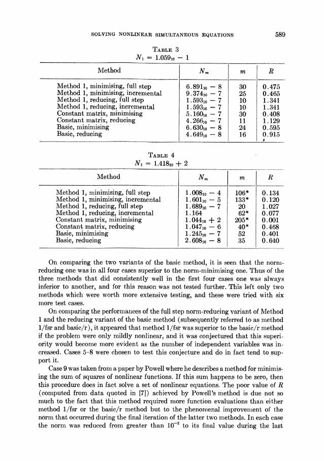
On comparing the two variants of the basic method, it is seen that the norni- reducing one was in all four cases superior to the norm-minimising one. Thus of the three methods that did consistently well in the first four cases one was always inferior to another, and for this reason was not tested further. This left only two methods which were worth more extensive testing, and these were tried with six more test cases.

On comparing the performances of the full step norm-reducing variant of Method 1 and the reducing variant of the basic method (subsequently referred to as method 1/fsr and basic/r), it appeared that method 1/fsr was superior to the basic/r method if the problem were only mildly nonlinear, and it was conjectured that this superi- ority would become more evident as the number of independent variables was in- creased. Cases 5-8 were chosen to test this conjecture and do in fact tend to sup- port it.

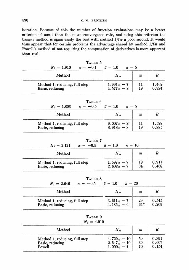
Case 9 was taken from a paper by Powell where he describes a miethod for minimis- ing the sum of squares of nonlinear functions. If this sum happens to be zero, then this procedure does in fact solve a set of nonlinear equations. The poor value of R (computed from data quoted in [7]) achieved by Powell's method is due not so much to the fact that this method required more function evaluations than either method 1/fsr or the basic/r method but to the phenomenal improvement of the norm that occurred during the final iteration of the latter two methods. In each case the norm was reduced from greater than 10-2 to its final value during the last

TABLE 3 N1 = 1.O591o - 1

Method Nm m R

Method 1, minimising, full step 6.8911o - 8 30 0.475 Method 1, minimising, incremental 9.37410 - 7 25 0.465 Method 1, reducing, full step 1. 5931o - 7 10 1.341 Method 1, reducing, incremental 1. 5931o - 7 10 1.341 Constant matrix, minimising 5.1601o - 7 30 0.408 Constant matrix, reducing 4.266l0 - 7 11 1.129 Basic, minimising 6.630io - 8 24 0.595 Basic, reducing 4.649jo - 8 16 0.915

TABLE 4 N1 - 1.418jo + 2

Method Nm m R

Method 1, minimising, full step 1. 0081o - 4 106* 0.134 Method 1, minimising, incremental 1. 6011o - 5 133* 0.120 Method 1, reducing, full step 1. 6891o - 7 20 1.027 Method 1, reducing, incremental 1. 164 62* 0.077 Constant matrix, minimising 1.0441o + 2 205* 0.001 Constant matrix, reducing 1. 0470 - 6 40* 0.468 Basic, minimising 1.2451o - 7 52 0.401 Basic, reducing 2.60810 - 8 35 0.640

590 C. G. BROYDEN

iteration. Because of this the number of function evaluations may be a better criterion of merit than the lmlean convergence rate, and using this criterion the basic/r method is again easily the best with method l/fsr a poor second. It would thus appear that for certain problems the advantage shared by method 1/fsr and Powell's method of not requiring the computation of derivatives is more apparent than real.

TABLE 5

N] = 1.910 a = -0.1 1.0 n 5

MVethod Nm m R

Method 1, reducing, full step 1.9lo - 7 11 1.462 Basic, reducing 4. 5771o - 8 19 0.924

TABLE 6 N1 = 1.803 a = -0.5 /=1.0 n 5

Method Nm m R

Method 1, reducing, full step 9.007,o - 8 11 1.528 Basic, reducing 8.918,o - 8 19 0.885

TABLE 7

N1 = 2.121 a = -0.5 ,3=1.0 n =10

Method Nm m R

Method 1, reducing, full step 1 . 597m0 - 7 18 0.911 Basic, reducing 2. 6021o - 7 34 0.468

TABLE 8

N1 = 2.646 a = -0.5 /3=1.0 n =20

Method Nm m R

Method 1, reducing, full step 3.611jo - 7 29 0.545 Basic, reducing 4. 185io - 6 64* 0.209

TABLE 9

N1 = 4.919

Method Nm m R

Method 1, reducing, full step 4.729wo - 10 59 0.391 Basic, reducing 2.547io - 10 39 0.607 Powell 1. 000o - 4 70 0.154

SOLVING NONLINEAR SIMULTANEOUS EQUATIONS 591

Case 10, for which no table is given, is due to Freudenstein and Roth. Both method 1/fsr and the basic/r methods failed to reach a solution although both came to grief at a point that proved to be a local minimum of the norm of f. Now the norm of f can be a minimum greater than zero only if the Jacobian matrix is singular at that point, and this contravenes one of the cardinal requirements for the success of Newton's method. For cases like this neither Newton's method nor any of its de- rivatives is likely to succeed and some radical innovation, like that due to Freuden- stein and Roth, is necessary.

10. Conclusions. From the discussion in the previous section the following con- clusions emerge.

(1) Norm reduction is a better strategy than norm minimisation. (2) If a reasonably good initial estimate of the solution is available method

1/fsr is superior to the basic/r method. (3) If a reasonably good initial estimate is not available then the basic/r method

is superior to method 1/fsr. Conclusions (2) and (3) are somewhat tentative, and the term "reasonably

good" is itself rather vague. Furthermore the behaviour of the various methods depends upon the nature of the problem they are attempting to solve, and it is thus unlikely that the few test problems selected give a sufficiently accurate picture of the overall behaviour of the algorithms to enable any more precise statements on the relative merits of the methods to be made. However, since method 1/fsr has never failed to converge when the basic/r method has converged and since for many of the test cases it was superior to the basic/r method, it may prove to be a useful alterna- tive, especially if a good initial estimate of Hi is available. This would occur in the method of Freudenstein and Roth or in solving a set of ordinary differential equa- tions by a predictor-corrector technique, when the corrector equations could be solved by Method 1 using as an initial estimate for Hi the final Hi obtained during the previous step.

Acknowledgments. The author is glad to acknowledge his indebtedness to Mr. F. Ford for reading the manuscript and making several valuable suggestions and to the directors of the English Electric Co. Ltd. for permission to publish this work.

Applied Analysis Section, Atomic Power Division English Electric Co. Ltd., Whetstone, Leicester, England.

APPENDIX 1. Summary of Method 1/far 1. Obtain an initial estimate xo of the solution. 2. Obtain an initial value Ho of the iteration matrix. This may be done either by

computing and inverting the Jacobian matrix, or it is possible that a sufficiently good approximation may be available from some other source, e.g. the final value of Hi from some previous calculation.

3. Compute fi = f(xi). 4. Compute pi Hifi.

592 C. G. BROYDEN

5. Select a value ti of t such that the norm of f(xi + tips) is less than the norm of f(xi). This is done iteratively and a modified version of the ALGOL procedure given in Appendix 2 may be used. In the course of this calculation the following will have been computed:

xi+, = xi + tip,,

ff+ = f(xi+1)

6. Test fj+j for convergence. If the iteration has not yet converged, then: 7. Compute y, = fi+1 -fi. 8. Compute H,+1 = H, - (H,yi + tipi)pi7H,/pi7Hiyi. 9. Repeat from step 4. I APPENDIx 2. The minimisation of the Euclidean norm of f regarded as a function

of the single variable t was carried out by a slightly modified version of the ALGOL procedure quadmin. The modifications enabled the procedure to perform some ad- ditional housekeeping operations and in no way affected the course of the iteration. On calling the procedure, the nonlocal variables n, last norm, x and p were set up as follows.

Nonlocal variable Value n Number of independent variables lastnorm f Tf

x Xi +pi p Pi

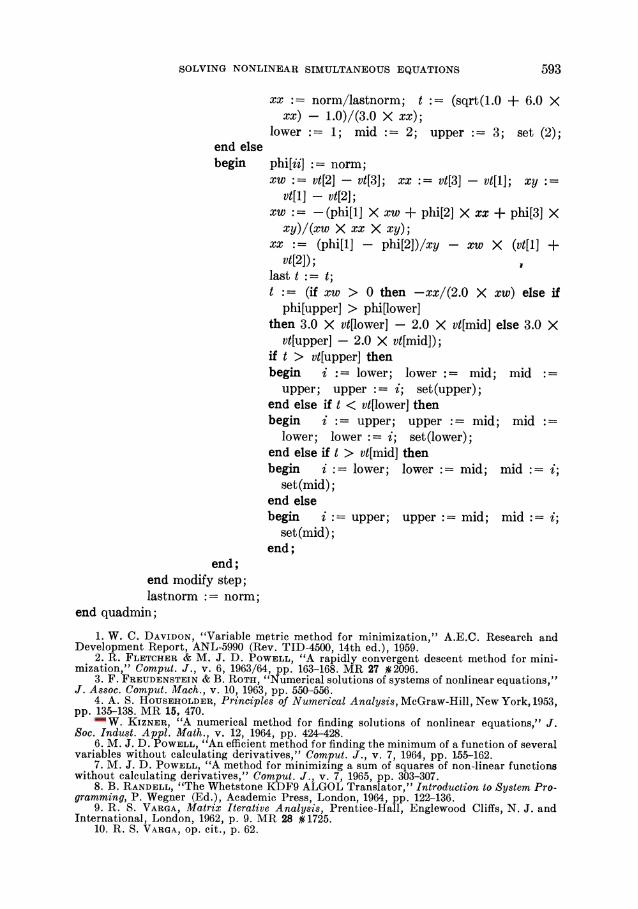
The procedure compute calculates the vector f(xi + tpi) for the current value of t, where xi + tpi is stored in the array x, and stores it in the nonlocal array f. The real procedure evalcrit computes the square of the Euclidean norm of the vector stored in the array f. On entry to quadmin t is set to zero to prevent premature emergence, but emergence is enforced when the number of iterations exceeds 10. procedure quadmin; begin comment This procedure minimises the Euclidean norm of the re-

siduals, treated as a function of the single variable t. Quadratic interpolation is used;

procedure set (i); value i; integer i; begin integer j;

ii : = i; vt[i] :=t; for j := 1 step I untl n do 41j] xUj] + (t - last t) X p[]; goto recompute;

end set; real xx, xw, xy, last t, norm; integer i, ii, upper, mid, lower, iterone; array phi, vt[1 :3]; last t := 1.0; t := 0; iterone := 0;

recompute: iterone := iterone + 1; compute; comment f now contains an approximation to f,+i; norm := evalcrit; if (abs(t - last t) > 0.01 X abs(t) and iterone S 10) or iterone = 2 then begin if iterone 1 then

begin vt[1] := 0; vt[3] := 1.0; phi[l] := lastnorm; phi[3] := norm;

SOLVING NONLINEAR SIMULTANEOUS EQUATIONS 593

xx := norm/lastnorm; t := (sqrt(l.0 + 6.0 X xx)- 1.0)/(3.0 X xx);

lower 1; mid 2; upper 3; set (2); end else begin phi[ii] = norm;

xw := vt[2] - vt[3]; xx vt[3] -vt[l]; xy vt[1] - vt[2];

xw := -(phi[l] X xw + phi[2] X xx + phi[3] X xy)/(xw X xx X xy);

xx : = (phi[1] - phi[2])/xy - xw X (vt[1] + vt[2]);

last t := t; t := (if xw > 0 then -xx/(2.0 X xw) else if

phi[upper] > phi[lower] then 3.0 X vt[lower] - 2.0 X vt[mid] else 3.0 X

vt[upper] - 2.0 X vt[mid]); if t > vt[upper] then begin i := lower; lower mid; mid

upper; upper := i; set(upper); end else if t < vt[lower] then begin i := upper; upper := mid; mid

lower; lower := i; set (lower); end else if t > vt[mid] then begin i := lower; lower := mid; mid :=i;

set(mid); end else begin i upper; upper mid; mid i;

set(mid); end;

end; end modify step; lastnorm := norm;

end quadmin;

1. W. C. DAVIDON, "Variable metric method for minimization," A.E.C. Research and Development Report, ANL-5990 (Rev. TID-4500, 14th ed.), 1959.

2. R. FLETCHER & M. J. D. POWELL, "A rapidly convergent descent method for mini- mization," Comput. J., v. 6, 1963/64, pp. 163-168. MR 27 ,2096.

3. F. FREUDENSTEIN & B. ROTH, "Numerical solutions of systems of nonlinear equations," J. Assoc. Comput. Mach., v. 10, 1963, pp. 550-556.

4. A. S. HOUSEHOLDER, Principles of Numerical Analysis, McGraw-Hill, New York, 1953, pp. 135-138. MR 15, 470.

5. W. KIZNER, "A numerical method for finding solutions of nonlinear equations," J. Soc. Indust. Appl. Math., v. 12, 1964, pp. 424-428.

6. M. J. D. POWELL, "An efficient method for finding the minimum of a function of several variables without calculating derivatives," Comput. J., v. 7, 1964, pp. 155-162.

7. M. J. D. POWELL, "A method for minimizing a sum of squares of non-linear functions without calculating derivatives," Comput. J., v. 7, 1965, pp. 303-307.

8. B. RANDELL, "The Whetstone KDF9 ALGOL Translator," Introduction to System Pro- gramming, P. Wegner (Ed.), Academic Press, London, 1964, pp. 122-136.

9. R. S. VARGA, Matrix Iterative Analysis, Prentice-Hall, Englewood Cliffs, N. J. and International, London, 1962, p. 9. MR 28 N 1725.

10. R. S. VARGA, op. cit., p. 62.