Solving Nonlinear Stochastic Growth Models: Comparison of

O 1990 American Statistical Association Journal of Business & Economic Statistics, January 1990, Vol. 8, No. 1

Associate Editor's Note: The following 11 articles summarize the efforts to date of a group that has been working on the new and exciting topic of solution strategies for nonlinear rational- expectations models. The members of the group wish to thank the National Bureau of Economic Research, the Institute for Empirical Macroeconomics, and the National Science Foundation for providing financial support for various aspects of the research activities. 1 wish to thank the many referees whose willingness to review the materials in a careful and timely manner helped im~rove the work substantially.

George Tauchen

Solving Nonlinear Stochastic Growth Models: A Comparison of Alternative Solution Methods John B. Taylor

Department of Economics, Stanford University, Stanford, CA 94305-601 0

Harald Uhlig Department of Economics, University of Minnesota, Minneapolis, MN 55455

The purpose of this article is to report on a comparison of several alternative numerical solution techniques for nonlinear rational-expectations models. The comparison was made by asking individual researchers to apply their different solution techniques to a simple representative- agent, optimal, stochastic growth model. Decision rules as well as simulated time series are compared. The differences among the methods turned out to be quite substantial for certain aspects of the growth model. Therefore, researchers might want to be careful not to rely blindly on the results of any chosen numerical solution method in applied work.

KEY WORDS: Linear-quadratic approximation; Nonlinear models; Numerical solution methods; Optimal growth; Rational expectations.

1. INTRODUCTION complex models and apply them to practical policy or other applied problems.

During the last few years, there has been an increased The purpose of this article is to report on a compar- demand for numerical solution methods for nonlinear ison of several alternative numerical solution techniques rational-expectations models. The demand has come for nonlinear rational-expectations models. All of the from economic researchers with diverse research goals techniques are currently under development and rely and modeling strategies. In almost all areas of macro- on high-speed computer technology or will eventually economics, rational-expectations models are becoming need this technology when they are moved beyond sim- increasingly complex and richer in structure. Empirical ple test problems. The comparison is one of the activities researchers studying real business-cycle models are at- of a research group called the Nonlinear Rational Ex- tempting to go beyond simple representative-agent pectations Modelling Group supported by the National models with convenient, but sometimes unrealistic, Bureau of Economic Research. Participants in the functional forms for the utility functions; they are also group meetings at Stanford and Minneapolis have in- beginning to study models with distortions and exter- cluded Marianne Baxter, Wilbur John Coleman, Law- nalities. Researchers focusing on monetary models are rence Christiano, Darrell Duffie, Ray Fair, Joseph finding it necessary to solve large nonlinear stochastic Gagnon, Lars Hansen, Beth Ingram, Kenneth Judd, systems to apply rational-expectations techniques to Pamela Labadie, David Luenberger, Rodolfo Manuelli, practical problems of monetary policy, including inter- Albert Marcet, Ellen McGrattan, David Runkle, John national monetary policy. Finance economists inter- Rust, Thomas Sargent, Christopher Sims, Kenneth Sin- ested in dynamic "consumption-beta" models are gleton, John Taylor, George Tauchen, and Harald finding it necessary to go beyond simple analytical Uhlig. The comparison was made by asking individual models to confront the theory with the data. As elec- researchers to apply different solution techniques to a tronic computing power becomes faster and cheaper, simple representative-agent, optimal, stochastic growth numerical solution procedures will enable macroecon- model designed to describe the behavior of aggregate omists and financial economists to study these more consumption and the capital stock. Though simple, the

2 Journal of Business & Economic Statistics, January 1990

problem does not have an analytic solution. Hence the solution results are of interest in their own right in addition to enabling a comparison of alternative methods.

Section 2 describes the stochastic growth model. Sec- tion 3 very briefly describes the solution methods. More details about each of the techniques are contained in articles by the individual authors that accompany this article. Section 4 presents the comparison of the different solution methods on the test problem. Section 5 considers issues for future research.

2. THE STOCHASTIC GROWTH MODEL

The following problem was proposed by Christopher Sims to be solved by the individual researchers. Let C, be consumption and Kt be the capital stock. Agents are assumed to maximize

subject to

and to the side conditions that Kt > 0 and C, > 0 for all t. Note that Equation (2 ) implies that there is no depreciation of the capital stock. A slightly more general formulation would have some depreciation in which a coefficient less than 1 would multiply the lagged value of the capital stock in Equation (2 ) . Agents at time t choose Kt and C,. Agents are assumed to know the history of all variables dated t and earlier when they choose variables dated t.

The stochastic process for 8, is given by

where E is a serially uncorrelated, normally distributed random variable with mean 0 and constant variance a$

For this problem, decision rules for consumption C, and the capital stock K, in any period t are given by the functions f ( K t _ 8,) and g(K, - I,8,) of the capital stock in period t - 1 and the random shock in period t. Exact solutions for f and g are not known for this problem. If the utility function is logarithmic ( T = 1) and there is full depreciation rather than zero depreciation as in Equation ( 2 ) , then there is a simple closed-form solution (e.g., see Sargent 1987, p. 122). For the problem in Equations ( 1 ) and ( 2 ) ,the functions f and g must be evaluated numerically.

To compare the different solution methods, the stochastic growth problem was solved for 10 cases of parameter values. The parameters for the 10 cases are given in Table 1 with a = .33 and p = .95 for all cases. These values of the coefficient of relative risk aversion ( 5 ) allow for considerable differences in the degree of risk aversion. Note also that the technology shock has a very large variance in cases 1-4, indicating a high degree of uncertainty.

Table 1. Parameter Choices for the 10 Cases

Case B 5 a,

Individual researchers reported results in two basic forms, decision rules ( f and g ) for consumption and capital and stochastic simulation paths for consumption and capital. The decision rules f and g were evaluated for a grid of values of capital and the technology shock. For the stochastic simulations, shocks on E , were drawn so as to generate a path for C, and K, over time.

3. THE SOLUTION METHODS

Ten researchers participated in the solution comparison by submitting decision rules andlor stochastic simulation paths. The names of the researchers, in alphabetical order, along with the type of method that each researcher used, an indication of whether decision rules were submitted, and the number of periods in the simulated time series submitted in each case are listed in Table 2.

A very brief overview of the general features of each method is provided for convenience here. Details of how these methods are implemented in the stochastic growth model can be found in the articles by the individual authors that accompany this article. To use the methods, one, of course, needs to read these articles.

Value-Function Grid. The basic idea here is to approximate the continuous valued-growth problem by a discrete-valued problem over a grid of points. In other words, the values of K and the shocks are discretized. By making the grid finer, the actual solution for K can be approximated arbitrarily closely. These approximations result in a discrete state-space dynamic optimization model that is solved by iterating on the value function. The finer the grid is, the more expensive will be the computation for this method. Higher dimensions for the control variable increase computation time greatly, but for the test problem there is only one dimension, and computing time is not a problem. Chris- tiano used this method to solve the growth problem in Equation (1 ) . See Christian0 (1990) for details.

Quadrature Value-Function Grid. This method also discretizes the state space, but it is potentially more efficient than the simple grid in that a quadrature rule is used to discretize the state space. Tauchen has applied this method successfully in several problems. See Tauchen (1987, 1990) for a description of the method and for a discussion of some applications.

3 Taylor and Uhlig: A Comparison of Alternative Solution Methods

Table 2. Summav of the Methods

Researcher Type of method

Baxter Euler-equation grid Christian0 Lin-LQ-Normal Christian0 Lin-LQ-discrete Christian0 Log-LQ-Normal Christian0 Log-LQ-discrete Christian0 Value-function grid Coleman Euler-equation grid Gagnon Extended path lngram Backsolving Labadie Least square projection Marcet Parameterizing expectations McGrattan Lin-LQ-Normal Sims Backsolving Tauchen Quadrature value-function grid

Linear-Quadratic (lin-LQ-Normal, fin-LQ-discrete, log-LQ-Normal, log-LQ-discrete). This method ap- proximates the control problem in Equation (1) with a standard linear-quadratic (LQ) control problem to which linear decision rules for K and C are optimal and can be computed easily. The linear decision rules are then treated as approximations to the exact solutions. The approximation is made by first substituting the constraint (2) into the objective function (1) and then making a quadratic approximation of the utility function at each time period. The approximation is taken about the steady-state values of the problem. This method was used by Kydland and Prescott (1982). Its application to the problem considered in this article is described by Christiano (1990) and McGrattan (1990).

In preparing calculations for the LQ method reported in this article, Christiano did four variants of this method. In one variant, log(K) was treated as a control variable, and in another variant, K was treated as a control variable. The two solutions are referred to as log-LQ and lin-LQ respectively. Moreover, for each of these two variants, Christiano drew the shocks in the stochastic simulations either according to a continuous- valued normal distribution or according to a discrete distribution. The identifiers "Normal" and "discrete" are used to indicate these two variants. The latter type of draws were made for comparison with the value- function-grid methods. McGrattan's LQ results are based on treating K as the control variable and drawing normal errors and, therefore, are referred to as the lin- LQ-Normal method in this article.

Backsolving. This method was proposed by Sims (1984, 1989). The implementation for the stochastic growth problem is described by Ingram (1990) and Sims (1990). The backsolving method is a general approach rather than a specific algorithm, and, in fact, the Ingram and Sims backsolving implementations are considerably different in this application. The backsolving method starts out by solving a problem that is more analyti- cally tractable than the actual problem and then ap- proximates the actual problem at the stage when the stochastic shocks are drawn. For example, in this

Decision Simulation rules periods Cases

Yes 2,009 All cases Yes 2,000 All cases Yes 2,000 All cases Yes 2,000 All cases Yes 2,000 All cases No 2,000 Cases 5-1 0 Yes 1,999 All cases Yes 500 All cases No 1,000 All cases No 680 Cases 1, 5, 7 Yes 1,649 All cases Yes 2,000 All cases No 2,000 All cases Yes 2,000 All cases

application Sims solves a linear-quadratic approximation to the original problem and draws shocks for the Euler equation, backsolving for the shocks in the pro- duction function. Ingram modifies the original problem by adding another shock with a convenient distribution, thus relaxing the budget constraint.

Extended Path. This method was described in general terms by Fair and Taylor (1983), and its implementation in the stochastic growth problem is described by Gagnon (1990). When applied to the optimal-control problems like the one in Equation (I), it works by solving the nonlinear dynamic first-order conditions that are implied from the discrete-time calculus-of-varia- tions formulation of the problem. These first-order conditions at time t involve conditional expectations of Kt+ , . These future expectations are solved out iteratively to solve the first-order conditions, thereby obtaining the decision rule solution for Kt. The decision rule for consumption is then computed from the budget identity. Atthough stochastic iterations may improve the accuracy of the method in some cases, only deterministic iterations were performed by Gagnon.

Euler-Equation Grid. Coleman's method and Bax- ter's method fall into this category. Coleman's method works by approximating the decision rules for con-sumption and capital (by piecewise linear functions, for example). Using these approximate functions, the method then iteratively solves the Euler equations directly rather than by iterating on the value function. Convergence is checked over a grid of values. [See Coleman (1990) and the references therein.] Baxter's method discretizes the state space and then iterates to find the value for capital, restricted to the grid, that comes closest to solving the Euler equations. [See Bax- ter, Crucini, and Rouwenhorst (1990) for the implementation of the method in the stochastic growth problem .]

Parameterizing Expectations. This method was originally proposed by Marcet (1988), and its implementation for the stochastic growth problem is described by Den Haan and Marcet (1990). Like the Euler-equation-grid and extended-path methods, this


method uses the first-order conditions (Euler equations) for the dynamic-optimization problem. The general idea is to hypothesize a general functional form with undetermined parameters for the conditional ex- pectation of future variables that appear in the first- order conditions. The parameters of this functional form are then "estimated" by least squares using a single set of simulated values. The functional form can then be generalized until convergence of the solution is achieved.

Least Squares Projections. This method was originally proposed by Labadie (1986), and its implementation for the stochastic growth problem is described by Labadie (1990). Like the method of parameterizing expectations, this method focuses on obtaining expres- sions for the conditional expectations implicit in the first-order conditions (Euler equations). It attempts to "estimate" certain parameters of the conditional expectations functions by using a single simulation of the random shocks in the model.

Counting the LQ methods only once, there are a total of eight different solution methods examined in this article, which reports on 14 different sets of solutions because there are four variants of the LQ method and because the backsolving method, the lin-LQ-Normal method, and the Euler-equation-grid method are each used by two researchers (though in some cases with a very different implementation procedure).

4. A COMPARISON OF THE RESULTS

As indicated previously, researchers reported results both in the form of decision rules and stochastic simulation paths. The stochastic simulation paths were plotted graphically and were also used to calculate several summary statistics to aid in the comparison of the solution algorithms. In the first part of this section, we discuss the plots of the simulation paths and then go on to discuss the decision rules and the summary statistics.

4.1 Plots of the Stochastic Simulations

The reported stochastic simulation paths for all 10 cases are available on request. Due to space limitations, we only report plots of a sample of cases here. These cases were selected with several criteria in mind-to include as many researchers as possible, to demonstrate differences in behavior most clearly, and to illustrate that the differences are not particular to just one case.

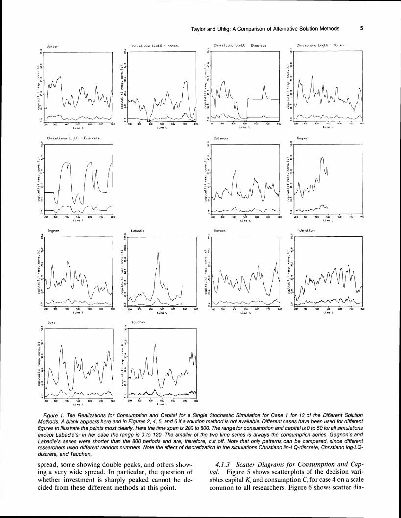
4.1.1 Time Series Charts. Figure 1 shows the realizations for consumption and capital for a single stochastic simulation for case 1 for 13 of the different solution methods. (To assist readers in scanning the figures, the charts in each figure are organized in the same order, and in cases in which a solution method is not available, a blank appears in the figure.) Note that each researcher used different sets of draws of the random variable so that the actual realizations will be

much different for each method. Even if two methods gave exactly the same accuracy, only the general patterns of the stochastic simulations would appear similar for the different methods. On an absolute basis, the level of consumption is, of course, much less than the level of the capital stock. The fluctuations in consumption are also smaller than the fluctuations in the capital stock. All of the methods show a high degree of con- temporaneous correlation between consumption and the level of capital. Most of the variance in both consumption and capital is in the low frequencies (assuming an annual time frame). The discretization of capital in Tauchen's method is quite evident, as is the resulting erratic behavior of consumption. Note also the en-counters with 0 in the lin-LQ-Normal simulation and the shock-and-convergence-back behavior in the lin- LQ-discrete simulation. But even aside from this "ex- otic" behavior, differences among the solution methods may be quite large: compare, for example, the plots for McGrattan's solution and Marcet's solution. Marcet's parameterizing-expectations solution finds a much higher variance for capital and a much lower frequency of fluctuations than does McGrattan's linear-quadratic method. The macroeconomic interpretations of these two simulations would be much different.

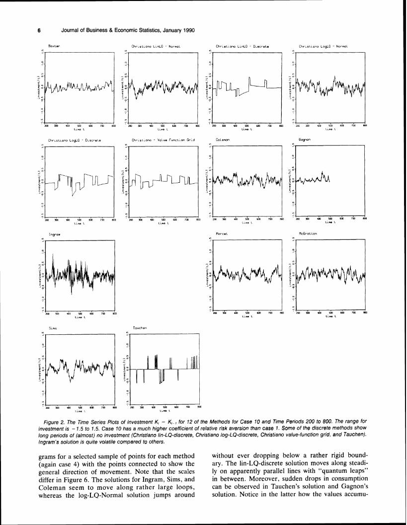
Figure 2 shows the time series plots of investment (Kt - Kt_,) for 12 of the methods for case 10. This case has a much higher coefficent of relative risk aversion and a much lower technology shock than case 1. This comparison also shows considerable differences be-tween the methods. Some of the methods in which the shocks are drawn discretely (Christiano-lin-LQ-dis- Crete, Christiano-value-function grid, and Tauchen) show long periods of no change in the investment series. Note that Ingram's solution appears to have a higher volatility of investment than the other methods.

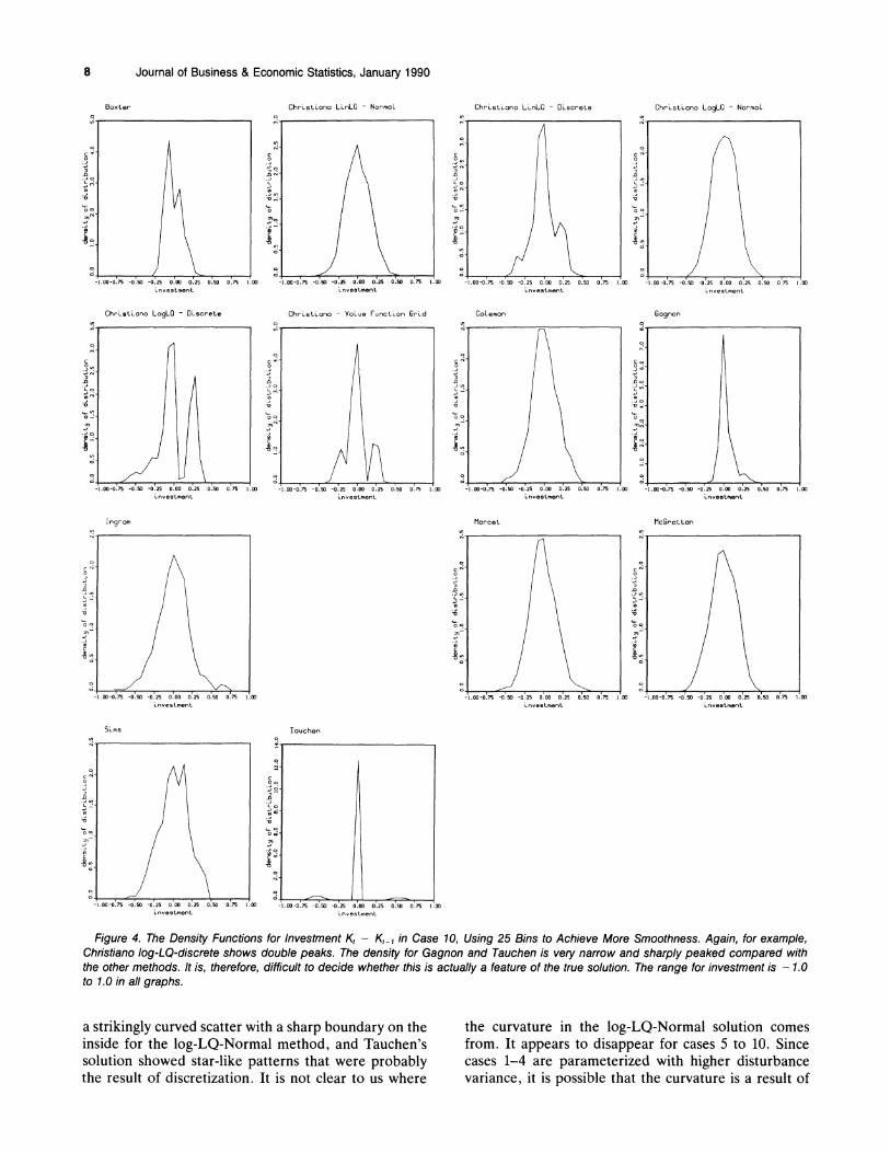
4.1.2 Empirical Density Functions for Consumption and Investment. In Figure 3, we present empirical density functions for consumption for case 5 (50 grid points), and in Figure 4, we present empirical density functions for investment for case 10 (25 grid points to achieve more smoothness). The density functions all integrate to 1, but notice the different vertical scales. (Frequently, a histogram is drawn as a step function with certain heights for each bin. Note however, that connecting these heights by straight lines, as we do in Figs. 3 and 4, results in a function with the same integral as the original step function if the boundary values are 0.)

As with the time series plots, the differences between the empirical density functions are quite striking. Ex-cept for those of Coleman and possibly McGrattan, none of the density functions are particularly smooth. Obviously, even with 2,000 simulated data points the variance on these estimated density functions is quite high. Nonetheless, the differences between the solutions are large with some methods showing very little


m ao +x m wo ,n aoo rm nn +x sao am ?m sm

Figure 1. The Realizations for Consumption and Capital for a Single Stochtistic Simulation for Case 1 for 13 of the Different Solution Methods. A blank appears here and in Figures 2, 4, 5, and 6 if a solution method is not available. Different cases have been used for different figures to illustrate the points most clearly. Here the time span is 200 to 800. The range for consumption and capital is 0 to 50 for all simulations except Labadie's; in her case the range is 0 to 120. The smaller of the two time series is always the consumption series. Gagnon's and Labadie's series were shorter than the 800 periods and are, therefore, cut off. Note that only patterns can be compared, since different researchers used different random numbers. Note the effect of discretization in the simulations Christiano lin-LQ-discrete, Christiano log-LQ- discrete, and Tauchen.

spread, some showing double peaks, and others show- 4.1.3 Scatter Diagrams for Consumption and Cap- ing a very wide spread. In particular, the question of ital. Figure 5 shows scatterplots of the decision vari- whether investment is sharply peaked cannot be de- ables capital K, and consumption C, for case 4 on a scale cided from these different methods at this point. common to all researchers. Figure 6 shows scatter dia-


B o x t e r C h r ~ r t i o n o - Normal - D ~ n c r e t e LogLOLmLO C h r ~ s l i a n aL L ~ L C C h r ~ r ~ ~ a n o - Normal

I , , , , ,m sn ao roo sw ma aoo m m oo roo am ~ r n sw m m an ux, sm Jrn sm 2oc mo t a o ioo 6W l w KO t i n e L t ~ n at LL". L Line L

Figure 2. The Time Series Plots of Investment K, - K, , for 72 of the Methods for Case 10 and Time Periods 200 to 800. The range for investment is - 1.5 to 1,5. Case 70 has a much higher coefficient of relative risk aversion than case 1. Some of the discrete methods show long periods of (almost) no investment (Christiano lin-LQ-discrete, Christiano log-LQ-discrete, Christiano value-function grid, and Tauchen). Ingram's solution is quite volatile compared to others.

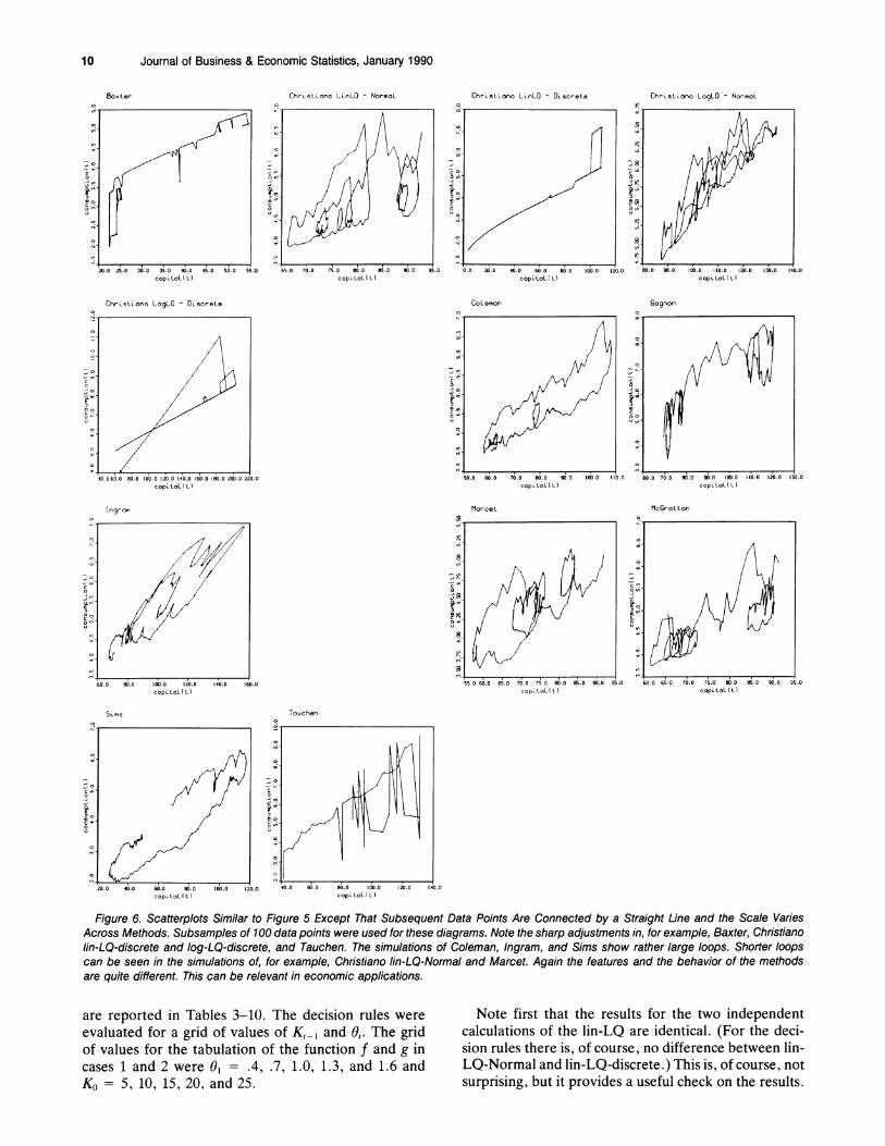
grams for a selected sample of points for each method without ever dropping below a rather rigid bound- (again case 4) with the points connected to show the ary. The lin-LQ-discrete solution moves along steadi- general direction of movement. Note that the scales ly on apparently parallel lines with "quantum leaps" differ in Figure 6. The solutions for Ingram, Sims, and in between. Moreover, sudden drops in consumption Coleman seem to move along rather large loops, can be observed in Tauchen's solution and Gagnon's whereas the log-LQ-Normal solution jumps around solution. Notice in the latter how the values accumu-


C h r ~ s L ~ o n oL L ~ L O- Norma l C h r ~ s t ~ a n oLogLO - Norm01

- 1.2 2 . 1 1.6 2 8 1.0 1.2 3 4 cmaunplron conrumptron consumption

Figure 3. The Empirical Density Functions for Consumption for Case 5 and for all Available Data of a Simulation. The range for consumption is 1.8 to 3.4 (actually, these numbers are rounded from the original bin bounds, which explains the cutoff in Ingram's graph). Fifty bins are used, and the heights are connected by a straight line; this still results in a density integrating to 1 if the boundary values are 0. Most density functions are surprisingly ragged. Some-for example, Christiano's discrete methods-show double peaks. The shapes vary considerably across methods, but it is possible that this is largely due to the rather small length of the simulated time series (mostly 2,000 data points).

late to two "islands." These islands are probably be- into a simple large scatter, as do most of the other cause Gagnon has provided a small sample of points. methods. Gagnon has reported that additional simulations (not re- Additional scatterplots not reported here show ad- ported here) show that more data points begin to fill ditional anomalies. For example, scatter diagrams of in the sparse areas and the scatter diagram develops investment versus the change in consumption showed


B o x t e r C h r ~ s L ~ a n a - No rma l L L ~ L O D ~ s c r e L e LoqLOL L ~ L O C h r ~ s t ~ o n a - C h r ~ s L ~ o n o - Normal

C h r ~ n t ~ a n oLogLO - D ~ s c r e L e - VoLve F u n c L ~ o n Coleman GagnanC h r ~ s t ~ o n o G r ~ d

Figure 4. The Density Functions for Investment K, - K,-,in Case 10, Using 25 Bins to Achieve More Smoothness. Again, for example, Christian0 log-LQ-discrete shows double peaks. The density for Gagnon and Tauchen is very narrow and sharply peaked compared with the other methods. It is, therefore, difficult to decide whether this is actually a feature of the true solution. The range for investment is - 1.0 to 1.0 in all graphs.

a strikingly curved scatter with a sharp boundary on the the curvature in the log-LQ-Normal solution comes inside for the log-LQ-Normal method, and Tauchen's from. It appears to disappear for cases 5 to 10. Since solution showed star-like patterns that were probably cases 1-4 are parameterized with higher disturbance the result of discretization. It is not clear to us where variance, it is possible that the curvature is a result of


Figure 5. Scatterplots of the Decision Variables, Capital K, Versus Consumption C,, in Case 4. A common scale is used for all researchers: 0 to 300 for capital and -4.0 to 12.0 for consumption. Note how a sharp boundary is visible in Christiano lin-LQ-Normal, Christiano log-LQ- Normal, and McGrattan-that is, in the most commonly used linear-quadratic methods. Observe that the points scatter around two "islands" in Gagnon's solution. Gagnon reports that this island structure starts to disappear with longer simulations.

the quadratic approximation. Since the linear-quadratic 4.2 Decision Rules method is probably one of the most commonly used methods, this is an important issue for future research. For 10 of the 14 methods, researchers reported de- These diagrams reveal large differences among the dif- cision rules Kt = f (Kt- I , 8,) and Cl = g ( K r -1 , 0,) for ferent methods. consumption and capital. The results for cases 1 and 2

Journal of Business & Economic Statistics, January 1990

C h r ~ s L ~ a n oL L ~ L O- Normal C h r ~ s L ~ o n o -LoqLO Normal

Coleman Gagnon

S ~ m s Touchen

Figure 6. Scatterplots Similar to Figure 5 Except That Subsequent Data Points Are Connected by a Straight Line and the Scale Varies Across Methods. Subsamples of 100data points were used for these diagrams. Note the sharp adjustments in, for example, Baxter, Christiano /in-LQ-discrete and log-LQ-discrete, and Tauchen. The simulations of Coleman, Ingram, and Sims show rather large loops. Shorter loops can be seen in the simulations of, for example, Christiano lin-LQ-Normal and Marcet. Again the features and the behavior of the methods are quite different. This can be relevant in economic applications.

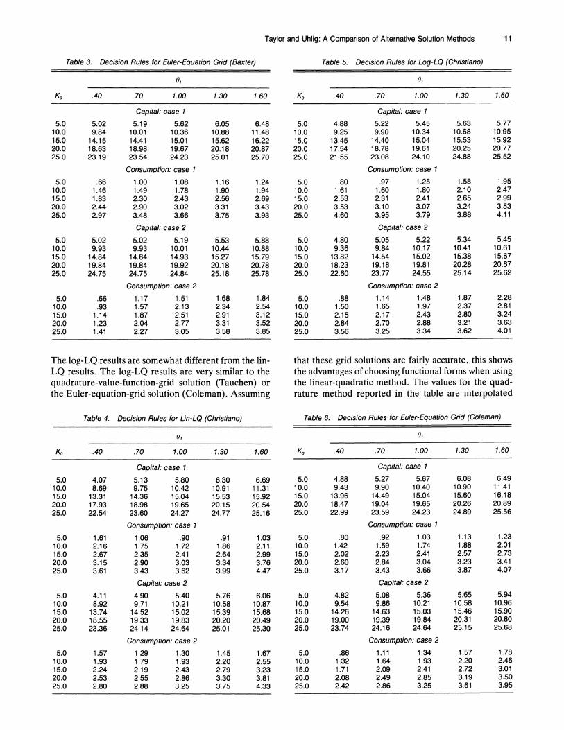
are reported in Tables 3-10. The decision rules were Note first that the results for the two independent evaluated for a grid of values of K,-, and 8,. The grid calculations of the lin-LQ are identical. (For the deci- of values for the tabulation of the function f and g in sion rules there is, of course, no difference between lin- cases 1 and 2 were 8, = .4, .7, 1.0, 1.3, and 1.6 and LQ-Normal and lin-LQ-discrete.) This is, of course, not KO = 5, 10, 15, 20, and 25. surprising, but it provides a useful check on the results.


Table 3. Decision Rules for Euler-Equation Grid (Baxter) Table 5. Decision Rules for Log-LO (Christiano)

Capital: case 1

5.19 5.62 10.01 10.36 14.41 15.01 18.98 19.67 23.54 24.23

Consumption: case 1

1 .OO 1.08 1.49 1.78 2.30 2.43 2.90 3.02 3.48 3.66

Capital: case 2

5.02 5.19 9.93 10.01

14.84 14.93 19.84 19.92 24.75 24.84

Consumption: case 2

1.17 1.51 1.57 2.13 1.87 2.51 2.04 2.77 2.27 3.05

The log-LQ results are somewhat different from the lin- LQ results. The log-LQ results are very similar to the quadrature-value-function-grid solution (Tauchen) or the Euler-equation-grid solution (Coleman). Assuming

Table 4. Decision Rules for Lin-LQ (Christiano)

Capital: case 1

5.13 5.80 6.30 9.75 10.42 10.91

14.36 15.04 15.53 18.98 19.65 20.15 23.60 24.27 24.77

Consumption: case 1

1.06 .90 .91 1.75 1.72 1.86 2.35 2.41 2.64 2.90 3.03 3.34 3.43 3.62 3.99

Capital: case 2

4.90 5.40 5.76 9.71 10.21 10.58

14.52 15.02 15.39 19.33 19.83 20.20 24.14 24.64 25.01

Consumption: case 2

1.29 1.30 1.45 1.79 1.93 2.20 2.19 2.43 2.79 2.55 2.86 3.30 2.88 3.25 3.75

Capital: case 7

5.22 5.45 9.90 10.34

14.40 15.04 18.78 19.61 23.08 24.10

Consumption: case 1

.97 1.25 1.60 1.80 2.31 2.41 3.10 3.07 3.95 3.79

Capital: case 2

5.05 5.22 9.84 10.17

14.54 15.02 19.18 19.81 23.77 24.55

Consumption: case 2

1.14 1.48 1.65 1.97 2.17 2.43 2.70 2.88 3.25 3.34

that these grid solutions are fairly accurate, this shows the advantages of choosing functional forms when using the linear-quadratic method. The values for the quadrature method reported in the table are interpolated

Table 6. Decision Rules for Euler-Equation Grid (Coleman)

01

KO .40 .70 7.00 1.30 1.60

Capital: case 7

Consumption: case 7

5.0 .80 .92 1.03 1.13 1.23 10.0 1.42 1.59 1.74 1.88 2.01 15.0 2.02 2.23 2.41 2.57 2.73 20.0 2.60 2.84 3.04 3.23 3.41 25.0 3.17 3.43 3.66 3.87 4.07

Capital: case 2

5.08 5.36 9.86 10.21

14.63 15.03 19.39 19.84 24.16 24.64

Consumption: case 2

1.1 1 1.34 1.64 1.93 2.09 2.41 2.49 2.85 2.86 3.25


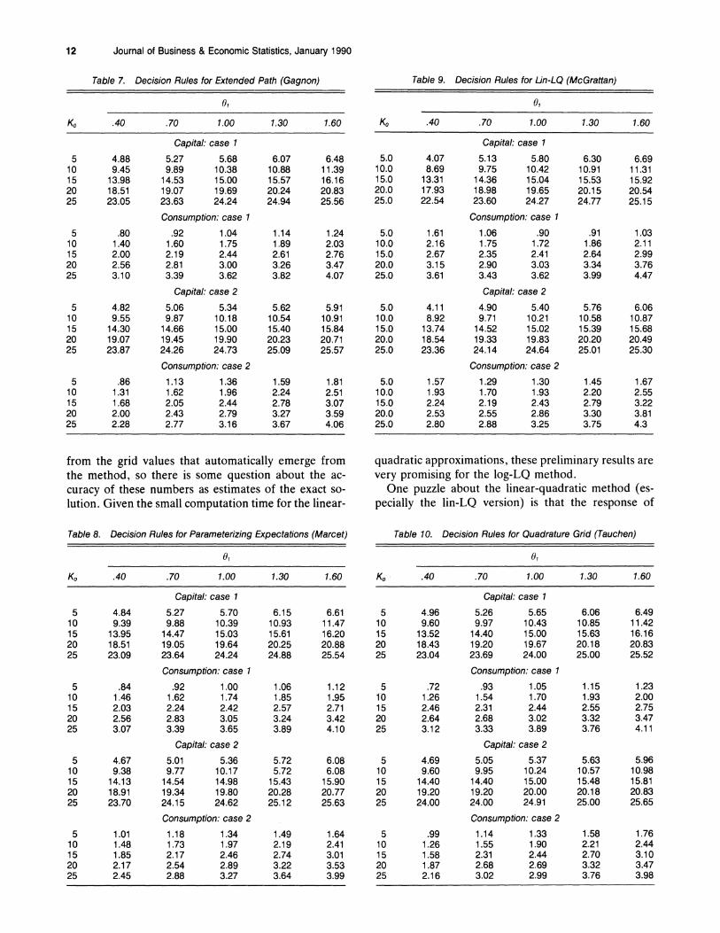
Table 7. Decision Rules for Extended Path (Gagnon)

KO .40 .70 7.00 1.30 1.60

Capital: case 1

Consumption: case 1

Capital: case 2

Consumption: case 2

from the grid values that automatically emerge from the method, so there is some question about the accuracy of these numbers as estimates of the exact solution. Given the small computation time for the linear-

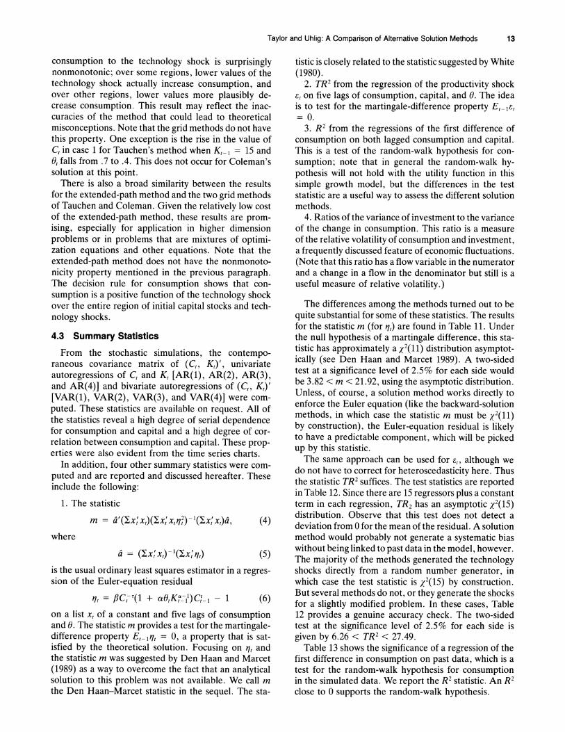
Table 8. Decision Rules for Parameterizing Expectations (Marcet)

01

Capital: case 1

5.27 5.70 9.88 10.39

14.47 15.03 19.05 19.64 23.64 24.24

Consumption: case 1

.92 1 .OO 1.62 1.74 2.24 2.42 2.83 3.05 3.39 3.65

Capital: case 2

5.01 5.36 9.77 10.17

14.54 14.98 19.34 19.80 24.15 24.62

Consumption: case 2

1.18 1.34 1.73 1.97 2.17 2.46 2.54 2.89 2.88 3.27

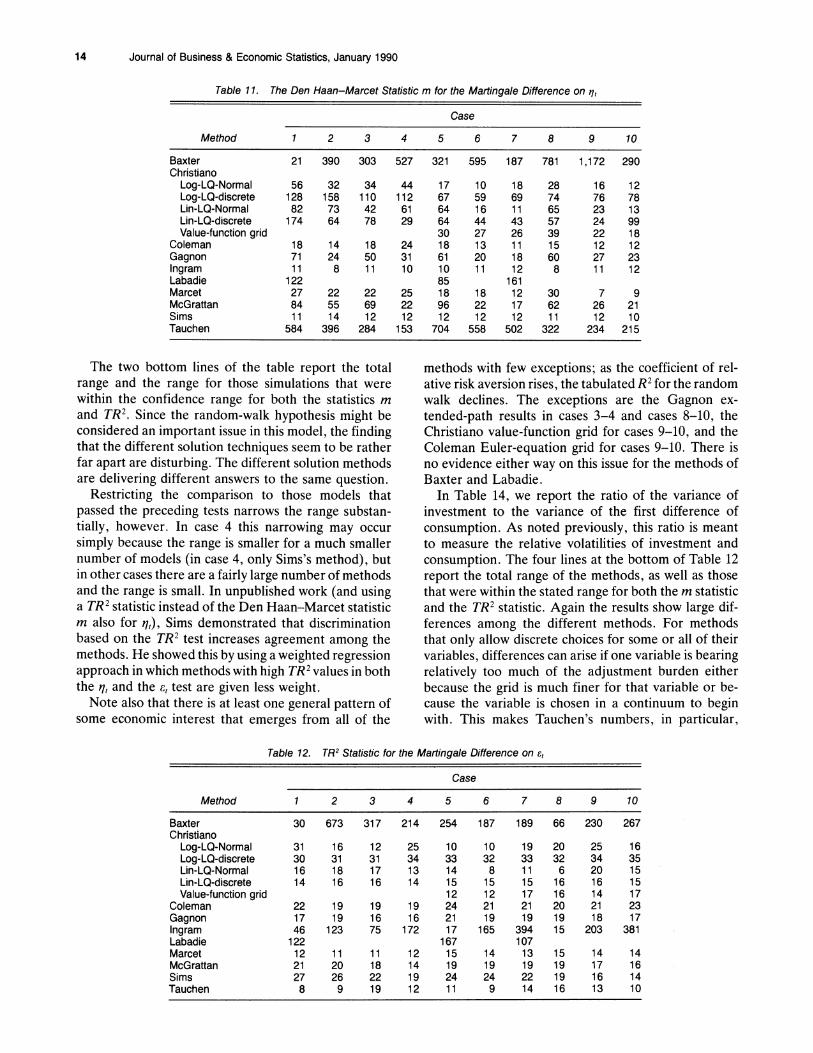
Table 9. Decision Rules for Lin-LQ (McGrattan)

Capital: case 1

Consumption: case 1

1.06 .90 1.75 1.72 2.35 2.41 2.90 3.03 3.43 3.62

Capital: case 2

4.90 5.40 9.71 10.21

14.52 15.02 19.33 19.83 24.14 24.64

Consumption: case 2

quadratic approximations, these preliminary results are very promising for the log-LQ method.

One puzzle about the linear-quadratic method (especially the lin-LQ version) is that the response of

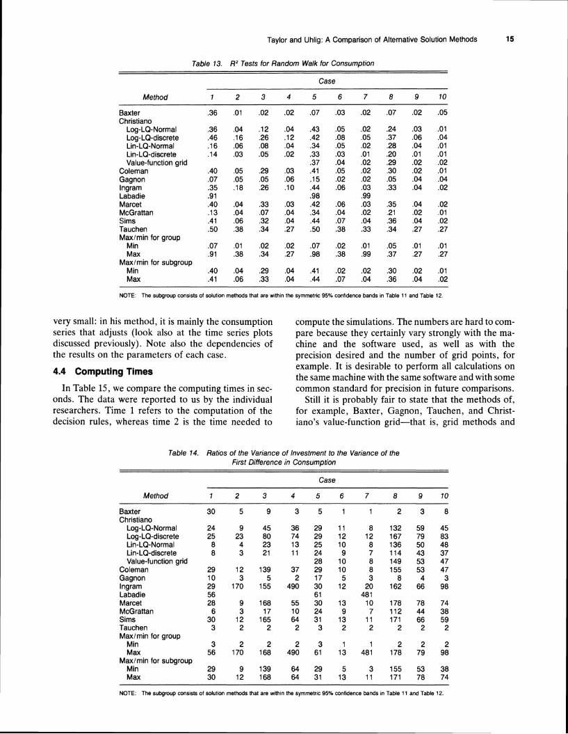
Table 10. Decision Rules for Quadrature Grid (Tauchen)

Capital: case 1

5.26 5.65 9.97 10.43

14.40 15.00 19.20 19.67 23.69 24.00

Consumption: case 1

.93 1.05 1.54 1.70 2.31 2.44 2.68 3.02 3.33 3.89

Capital: case 2

5.05 5.37 9.95 10.24

14.40 15.00 19.20 20.00 24.00 24.91

Consumption: case 2

1.14 1.33 1.55 1.90 2.31 2.44 2.68 2.69 3.02 2.99


consumption to the technology shock is surprisingly nonmonotonic; over some regions, lower values of the technology shock actually increase consumption, and over other regions, lower values more plausibly de- crease consumption. This result may reflect the inac- curacies of the method that could lead to theoretical misconceptions. Note that the grid methods do not have this property. One exception is the rise in the value of C, in case 1 for Tauchen's method when K,-, = 15 and 8, falls from .7 to .4. This does not occur for Coleman's solution at this point.

There is also a broad similarity between the results for the extended-path method and the two grid methods of Tauchen and Coleman. Given the relatively low cost of the extended-path method, these results are promising, especially for application in higher dimension problems or in problems that are mixtures of optimization equations and other equations. Note that the extended-path method does not have the nonmonoto- nicity property mentioned in the previous paragraph. The decision rule for consumption shows that con-sumption is a positive function of the technology shock over the entire region of initial capital stocks and technology shocks.

4.3 Summary Statistics

From the stochastic simulations, the contempo-raneous covariance matrix of (C,, K,)', univariate autoregressions of C, and K, [AR(l), AR(2), AR(3), and AR(4)J and bivariate autoregressions of (C,, K,)' [VAR(l), VAR(2), VAR(3), and VAR(4)J were computed. These statistics are available on request. All of the statistics reveal a high degree of serial dependence for consumption and capital and a high degree of correlation between consumption and capital. These properties were also evident from the time series charts.

In addition, four other summary statistics were computed and are reported and discussed hereafter. These include the following:

1. The statistic

where

is the usual ordinary least squares estimator in a regression of the Euler-equation residual

on a list x, of a constant and five lags of consumption and 8. The statistic m provides a test for the martingale- difference property E,-,q, = 0, a property that is sat- isfied by the theoretical solution. Focusing on q, and the statistic m was suggested by Den Haan and Marcet (1989) as a way to overcome the fact that an analytical solution to this problem was not available. We call m the Den Haan-Marcet statistic in the sequel. The sta-

tistic is closely related to the statistic suggested by White (1980).

2. TR2 from the regression of the productivity shock E , on five lags of consumption, capital, and 0. The idea is to test for the martingale-difference property = 0.

3. R2 from the regressions of the first difference of consumption on both lagged consumption and capital. This is a test of the random-walk hypothesis for consumption; note that in general the random-walk hypothesis will not hold with the utility function in this simple growth model, but the differences in the test statistic are a useful way to assess the different solution methods.

4. Ratios of the variance of investment to the variance of the change in consumption. This ratio is a measure of the relative volatility of consumption and investment, a frequently discussed feature of economic fluctuations. (Note that this ratio has a flow variable in the numerator and a change in a flow in the denominator but still is a useful measure of relative volatility.)

The differences among the methods turned out to be quite substantial for some of these statistics. The results for the statistic m (for q,) are found in Table 11. Under the null hypothesis of a martingale difference, this statistic has approximately a %'(11) distribution asymptot- ically (see Den Haan and Marcet 1989). A two-sided test at a significance level of 2.5% for each side would be 3.82 < m < 21.92, using the asymptotic distribution. Unless, of course, a solution method works directly to enforce the Euler equation (like the backward-solution methods, in which case the statistic m must be %?(11) by construction), the Euler-equation residual is likely to have a predictable component, which will be picked up by this statistic.

The same approach can be used for E,, although we do not have to correct for heteroscedasticity here. Thus the statistic TR2 suffices. The test statistics are reported in Table 12. Since there are 15 regressors plus a constant -term in each regression, TR2 has an asymptotic x2(15) distribution. Observe that this test does not detect a deviation from 0 for the mean of the residual. A solution method would probably not generate a systematic bias without being linked to past data in the model, however. The majority of the methods generated the technology shocks directly from a random number generator, in which case the test statistic is ~'(1.5) by construction. But several methods do not, or they generate the shocks for a slightly modified problem. In these cases, Table 12 provides a genuine accuracy check. The two-sided test at the significance level of 2.5% for each side is given by 6.26 < TR2 < 27.49.

Table 13 shows the significance of a regression of the first difference in consumption on past data, which is a test for the random-walk hypothesis for consumption in the simulated data. We report the R2 statistic. An R2 close to 0 supports the random-walk hypothesis.

14

10

Journal of Business & Economic Statistics, January 1990

Table 11. The Den Haan-Marcet Statistic m for the Martingale Difference on v t

Case

Method 1 2 3 4 5 6 7 8 9

Baxter Christiano

Log-LQ-Normal Log-LQ-discrete Lin-LQ-Normal Lin-LQ-discrete Value-function grid

Coleman Gagnon lngram Labadie Marcet McGrattan Sims Tauchen

The two bottom lines of the table report the total methods with few exceptions; as the coefficient of rel- range and the range for those simulations that were ative risk aversion rises, the tabulated R2for the random within the confidence range for both the statistics m walk declines. The exceptions are the Gagnon ex-and TR2.Since the random-walk hypothesis might be tended-path results in cases 3-4 and cases 8-10, the considered an important issue in this model, the finding Christiano value-function grid for cases 9-10, and the that the different solution techniques seem to be rather Coleman Euler-equation grid for cases 9-10. There is far apart are disturbing. The different solution methods no evidence either way on this issue for the methods of are delivering different answers to the same question. Baxter and Labadie.

Restricting the comparison to those models that In Table 14, we report the ratio of the variance of passed the preceding tests narrows the range substan- investment to the variance of the first difference of tially, however. In case 4 this narrowing may occur consumption. As noted previously, this ratio is meant simply because the range is smaller for a much smaller to measure the relative volatilities of investment and number of models (in case 4, only Sims's method), but consumption. The four lines at the bottom of Table 12 in other cases there are a fairly large number of methods report the total range of the methods, as well as those and the range is small. In unpublished work (and using that were within the stated range for both the m statistic a TR2statistic instead of the Den Haan-Marcet statistic and the TR2statistic. Again the results show large dif- m also for q),Sims demonstrated that discrimination ferences among the different methods. For methods based on the TR2test increases agreement among the that only allow discrete choices for some or all of their methods. He showed this by using a weighted regression variables, differences can arise if one variable is bearing approach in which methods with high TR2values in both relatively too much of the adjustment burden either the q, and the E, test are given less weight. because the grid is much finer for that variable or be-

Note also that there is at least one general pattern of cause the variable is chosen in a continuum to begin some economic interest that emerges from all of the with. This makes Tauchen's numbers, in particular,

Table 12. TRZ Statistic for the Martingale Difference on 8 ,

Case

Method 1 2 3 4 5 6 7 8 9 1 0

Baxter 30 673 317 214 254 187 189 66 230 267 Christiano

Log-LQ-Normal 31 16 12 25 10 10 19 20 25 16 Log-LQ-discrete 30 31 31 34 33 32 33 32 34 35 Lin-LQ-Normal 16 18 17 13 14 8 11 6 20 15 Lin-LQ-discrete 14 16 16 14 15 15 15 16 16 15 Value-function grid 12 12 17 16 14 17

Coleman 22 19 19 19 24 21 21 20 21 23 Gagnon 17 19 16 16 21 19 19 19 18 17 lngram 46 123 75 172 17 165 394 15 203 381 Labdie 122 167 107 Marcet 12 11 11 12 15 14 13 15 14 14 McGrattan 21 20 18 14 19 19 19 19 17 16 S~ms 27 26 22 19 24 24 22 19 16 14 Tauchen 8 9 19 12 11 9 14 16 13 10

Taylor and Uhlig: A Comparison of Alternative Solution Methods 15

Table 13. R2 Tests for Random Walk for Consumption

Case

Method 1 2 3 4 5 6 7 8 9 1 0

Baxter Christiano


Coleman Gagnon lngram Labadie Marcet McGrattan Sims Tauchen Maximin for group

Min Max

Maximin for subgroup Min Max

NOTE. The subgroup conslsts of solution methods that are w~thin the symmetric 95% conf~dence bands in Table 11 and Table 12

very small: in his method, it is mainly the consumption compute the simulations. The numbers are hard to com- series that adjusts (look also at the time series plots pare because they certainly vary strongly with the ma- discussed previously). Note also the dependencies of chine and the software used, as well as with the the results on the parameters of each case. precision desired and the number of grid points, for

4.4 Computing Times example. It is desirable to perform all calculations on the same machine with the same software and with some

In Table 15, we compare the computing times in sec- common standard for precision in future comparisons. onds. The data were reported to us by the individual Still it is probably fair to state that the methods of, researchers. Time 1 refers to the computation of the for example, Baxter, Gagnon, Tauchen, and Christ- decision rules, whereas time 2 is the time needed to iano's value-function grid-that is, grid methods and

Table 14. Ratios of the Variance of Investment to the Variance of the First Difference in Consumption

Case

Method 1 2 3 4 5 6 7 8 9 10

Baxter Christiano


Coleman Gagnon lngram Labadie Marcet McGrattan Sims Tauchen Maximin for group

Min Max

Maxlmin for subgroup Min Max

NOTE: The subgroup consists of solution methods that are within the symmetric 95% confidence bands in Table 11 and Table 12.


Table 15. Computing Times

Method Machine Co-chip Megahertz Software Time 1 Time 2 -

Baxter IBM PS2-80 80287 16 FORTRAN 3 31 1,1880 Matlab 3 13 1640

Chr~st~ano Log-LQ-Normal Amdahl 5860 244 RATS Total 6 Log-LQ-d~screte Amdahl 5860 244 RATS Total 1 2 Lln-LQ-Normal Amdahl 5860 244 RATS Total 6 Lln-LQ-d~screte Amdahl 5860 244 RATS Total 1 2 Value-funct~on gr~d Amdahl 5860 IBM FORTRAN 1 4 1 Total 5 hours

Coleman Amdahl5890-300 VS-FORTRAN 2 3 11092 32 Gagnon Amdahl 5850 TROLL 13 0 396 5,320 lngram HP Vectra ESl12 80287 12110 GAUSS 2 0 Total 72 01 Labadle IBM Model 30 Yes GAUSS 1 496 Total 4 hours Marcet Compaq 386125 We~tek 25 R McFarland FORTRAN Total 60 McGrattan Compaq 386120 We~tek 11 67 20 Matlab 3 25 Total 0 7 S~ms Dell System 310 80386 20 MICROSOFT C 20 107 Tauchen Compaq 386125 80387-25 25 GAUSS 1 49b Total 2,768

NOTE T~meIrefers to the central processing unlt (CPU) t~meIn seconds to compute the declslon rule for one case (typlcally case 1) T~me2 refers to the CPU tlme In seconds to Compute a slrnulat~onof 2 000 data polnts for one case (typlcally case 1) The term total ~nd~catesthat the sum of time 1 and tlme 2 IS glven In Chrlstlano s value-functlon grld 20 000 grld polnts were used

the extended-path method-are computationally quite martingale-difference tests for the Euler-equation re- involved, whereas linear-quadratic methods are typi- sidual, however. cally quite fast for the simple stochastic growth model. 3. Summary statistics, which researchers might typ-

One should recognize that differences in computing ically examine to test theoretical hypotheses, are sig- costs can be enormous once the problem at hand goes nificantly different for many of the solution methods, beyond only a few dimensions and the "curse of di- even though the theoretical problem solved is exactly mensionality" starts to matter. It might be quite im- the same for each method. For example, the solution possible to compute the solution for a model with 15 methods give very different answers to basic questions state variables, say, using some grid method. Methods concerning the relative volatility of investment and con- that work with linear-quadratic approximation or pa- sumption. There is some similarity among the methods rameterizing expectations (including backsolving) or ex- in detecting the effects of risk aversion on random-walk tended-path methods will still be available at reasonable consumption behavior, however, and the methods that costs for these problems, however. satisfy both the Den Haan-Marcet test for the accuracy

of the Euler equation and the TR2 test for the distri- 5. CONCLUSION bution of the disturbance term-Sims's backsolving im-

plementation, Marcet's parameterizing-expectations The conclusions from this comparison of different method, and Coleman's Euler-equation iteration

solution techniques for nonlinear rational-expectations method-produce similar summary statistics and plots. models can be summarized briefly as follows. Given these large differences in the solution methods,

1. The simulated sample paths generated by the dif- the most obvious question is who won? Unfortunately, ferent solution methods have significantly different this question is still very difficult to answer, the criteria properties. Although certain common time series fea- of success for the solution methods are different. For tures of the behavior of consumption and investment some researchers, the appropriate measuring stick emerge from time series plots for all the methods, other might be the closeness of the numerical solution to the features show up in the empirical density functions and true decision rule. Grid methods are likely to do very scatter diagrams that reveal quite different behavior well here, and we noted that the log-LQ and the ex- even though the same model is being solved by each tended-path methods come close to the grid methods method. in terms of the decision rules. For others, it is computing

2. The decision rules indicate that some of the easily time that is most important, as long as the results are computed rules-the linear-quadratic (log-LQ) method within reason. This might be the case for estimation and the extended-path method-are fairly close to the applications or with applications with a large number "exact" decision rule as represented here by the quad- of state variables. Applications of this type can poten- rature-value-function-grid method of Tauchen or the tially exhibit financially significant savings in computing Euler-equation grid method of Coleman. Given the rel- time when solved with methods that work with linear- atively low computation times for these methods and quadratic approximations or parameterization of the their relatively easy generalization to higher dimen- expectations or extended-path methods instead of one sions, it is important to establish whether this property of the grid methods. In other applications, it might be holds up in other problems. Neither the log-LQ nor the important to be accurate with respect to first-order con- extended-path method performs particularly well in the ditions to test, for example, asset-pricing relationships;


Sims's backsolving method or Marcet's parameter-izing-expectations method are likely to perform very well in this respect. Finally, the level of difficulty and the judgment required to implement a particular method can be of great importance to the practi-tioner.

The comparisons performed previously did not single out one or several of the methods as performing at the very top in every respect. For a researcher who wants to select one of the techniques, it seems important to consider the particular problem and the budget constraint. Researchers might want to be careful not to use any solution method blindly hoping that the results are within acceptable bounds. An article that relies pri- marily on one method could include at least a partial set of results using an alternative, preferably unrelated method as an accuracy check and a diagnostic of po- tential areas where results or inference might be dis- torted. For example, a researcher who uses linear-quadratic methods might want to compare the results to those from some grid method for a few simple cases. Tests like the Den Haan-Marcet statistic seem reasonable as an additional diagnostic device. More checks of this type are desirable.

Even in a simple model such as that considered in this article, the different solution methods can yield quite different econometric results. It is essential to get a better understanding of where these differences come from and how big they can be in a particular application before relying too much on conclusions drawn from these solution methods.

ACKNOWLEDGMENTS

Taylor's research was supported by a grant from the National Science Foundation (NSF) at the National Bu- reau of Economic Research (NBER) and by the Stan- ford Center for Economic Policy Research. Uhlig's research was performed at the Institute for Empirical Macroeconomics, supported jointly by the Federal Re- serve Bank of Minneapolis, the University of Minne- sota. and NSF Grant SES-8722451. This article reports on results from solution algorithms developed and pre- sented at a series of meetings of the Nonlinear Rational Expectations Modelling Group at Stanford and Min- neapolis, supported by the NBER and the Institute for Empirical Macroeconomics. The article is meant to accompany 10 short papers describing the solution methods by (a) Marianne Baxter, Mario Crucini, and K. Geert Rouwenhorst, (b) Lawrence Christiano, (c) Wil- bur John Coleman, (d) Joseph Gagnon. (e) Beth Fisher Ingram, (f) Wouter J. den Haan and Albert Marcet, (g) Pamela Labadie, (h) Ellen McGrattan. (i) Chris- topher Sims. and ( j ) George Tauchen. Sims suggested the sample economic problems discussed in the article. We are grateful to members of the Nonlinear Rational Expectations Modelling Group. especially Lawrence Christiano. Albert Marcet, Ellen McGrattan. Christo- pher Sims, and George Tauchen. for help and sugges-

tions about the calculations. summary statistics, tables, and graphs. We also thank two anonymous referees for several valuable suggestions.

[Recerr'etl December 1988.1

REFERENCES

Baxtrr. M.. Crucini. M. J . . and Rouwenhorst. K. G . (1990). "Solving the Stochastic Growth Model by a Discrete-State-Space. Euler- Equatlon Approach." Journal of Burinerr and Ecorlomic Stutirtics, 8. 19-21.

Christiano. L. J . (1990). "Solving the Stochastic Growth Model by Linear-Quadratic Approximation and by Value-Function Itera-tion." Jo~rrnrrl o f Bltriness rrnd Economic Strrtistics. 8. 23-26.

Coleman. W. J.. I1 (1990). "Solving the Stochastic Growth Model by Policy-Function Iteration." Jourrlal qf'Btrstnerr und Economic Sta- tistics. 8. 27-29.

Den I-laan. W. J . . and Marcet. A . (1989). "Accuracy In Simulations." unpublished manuscript. Carnegie-Mellon University. Graduate School of Industrial Administration. -(1990). "Solving the Stochastic Growth Model by Parame-

terizing Expectations." Journal o f Businers and Economic Strrtis- tics. 8. 31-34.

F a r . R. C. . and Taylor. J . B. (1983). "Solution and Maximum Like- lihood Estimation of Dynamic Nonlinear Rational Expectations Models." Econometricrr, 51, 1169-1 1x5.

Gagnon. J . E . (1990). "Solving the Stochastic Growth Model by Deterministic Extended Path." Jo~trnrrl of Business and Economic Strrrisrics. 8. 35-36.

Inpram. B. F. (1990). "Solving the Stochastic Growth Model by Back- solving With an Expanded Shock Space." Jourrlrrl of Business and Econotnrc Statistics. 8. 37-38.

Kydland. F.. and Prescott, E . (1982). "Time to Build and Aggregate Fluctuations." Ecotlometrica. 50. 1315-1370.

Labadie. P. (19x6). "Solving Nonlinear Rational Expectations Models for Estimation: An Application to an Asset Pricing Model With Currency." unpublished manuscript. Columbia University. Grad- uate School of Business. -(1990). "Solving the Stochastic Growth Model by Using a

Recursive Mapping Based on Least Squares Projection." Jo~trrlul of B~rsir~ess clnd Economic Sratirtics. 8. 39-40.

Marcet. A. (1988). "Solving Non-linear Models by Parameterizing Expectations." unpublished manuscript. Carnegie-Mellon Univer- sity. Graduate School of Industrial Administration.

McGrattan. E . (1990). "Solving the Stochastic Growth Model by Linear-Quadratic Approximation." Jo~trnal of Businers and Eco- nomic Stutistics, X. 41-44,

Sargent. T. J. (1987). Dxnamic Macroecotlomic Tlzeory, Cambridge. MA: Harvard University Press.

Sims. C. A. (1983). "Solving Nonlinear Stochastic Equilibrium Models 'Backwards'." unpublished manuscript. University of Minnesota. Dept. of Economics. -(1989). "Solving Nonlinear Stochastic Optimization and Equi-

librium Problems Backwards," Discussion Paper 15, Institute for Empirical Macroeconomics, Federal Reserve Bank of Min- neapolis. -(1990). "Solving the Stochastic Growth Model by Backsolving

With a Particular Nonlinear Form for the Decision Rule," Jo~trnul of Business and Economic Stutistics, 8, 45-47.

Tauchen. G. (1987), "Quadrature-Based Methods for Obtaining Ap- proximate Solutions to Nonlinear Asset Pricing Models," technical report, Duke University, Dept. of Economics. -(1990), "Solving the Stochastic Growth Model by Using Quad-

rature Methods and Value-Function Iterations." Journul of Busi- ness and Economic Statistics, 8, 49-51.

White, H . (1980), "A Heteroskedasticity-Consistent Covariance Ma- trix Estimator and a Direct Test for Heteroskedasticity," Econo-metrica, 38. 817-839.

Documents

Solving Nonlinear Stochastic Growth Models: Comparison of