Embed Size (px)
Citation preview
A CLASS OF CONTRACTIVITY PRESERVING
HERMITE–BIRKHOFF–TAYLOR HIGH ORDER TIME
DISCRETIZATION METHODS
Abdulrahman Karouma
Thesis Submitted to the Faculty of Graduate and Postdoctoral Studies
In partial fulfilment of the requirements for the degree of Doctor of Philosophy in
Mathematics 1
Department of Mathematics and Statistics
Faculty of Science
University of Ottawa
c© Abdulrahman Karouma, Ottawa, Canada, 2015
1The Ph.D. program is a joint program with Carleton University, administered by the Ottawa-Carleton Institute of Mathematics and Statistics
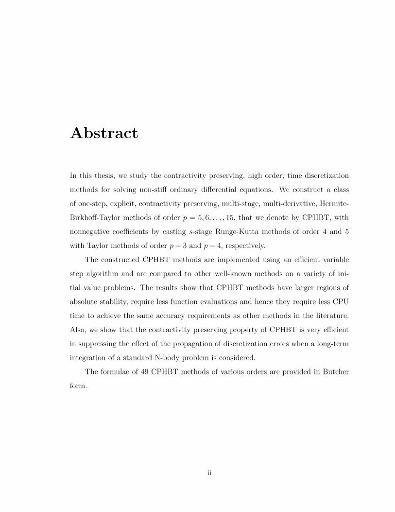
Abstract
In this thesis, we study the contractivity preserving, high order, time discretization
methods for solving non-stiff ordinary differential equations. We construct a class
of one-step, explicit, contractivity preserving, multi-stage, multi-derivative, Hermite-
Birkhoff-Taylor methods of order p = 5, 6, . . . , 15, that we denote by CPHBT, with
nonnegative coefficients by casting s-stage Runge-Kutta methods of order 4 and 5
with Taylor methods of order p− 3 and p− 4, respectively.
The constructed CPHBT methods are implemented using an efficient variable
step algorithm and are compared to other well-known methods on a variety of ini-
tial value problems. The results show that CPHBT methods have larger regions of
absolute stability, require less function evaluations and hence they require less CPU
time to achieve the same accuracy requirements as other methods in the literature.
Also, we show that the contractivity preserving property of CPHBT is very efficient
in suppressing the effect of the propagation of discretization errors when a long-term
integration of a standard N-body problem is considered.
The formulae of 49 CPHBT methods of various orders are provided in Butcher
form.
ii
Resume
Dans cette these, nous etudions des solveurs numeriques d’ordre eleve, qui preserve
la propriete de contractivite pour resoudre des equations differentielles ordinaires
non-raides. Nous construisons une classe de methodes explicites, multi-etage, multi-
derivees, Hermite-Birkhoff-Taylor d’ordre p = 5, 6, . . . , 15, a un pas. Ces methodes
sont a coefficients positifs ou nuls et combinent des methodes Runge-Kutta a s-etages
d’ordre 4 et 5 et des methodes de Taylor d’ordre p− 3 et p− 4, respectivement.
Ces methodes sont implementees en utilisant un algorithme efficace a pas vari-
able. Nous les comparons aux autres methodes bien connues pour des problemes
standards. Nos resultats montrent que les methodes CPHBT ont des regions de sta-
bilite absolue plus grandes, qu’elles necessitent moins d’evaluations de fonction et,
donc, sont plus rapides que les autres methodes connues. Nous montrons, de plus,
que la propriete de preservation de la contractivite de CPHBT supprime tres efficace-
ment l’effet de la propagation des erreurs de discretisation dans les integrations a long
terme des problemes standards a N-corps.
Les formules des 49 methodes CPHBT de divers ordres sont fournies sous la
forme Butcher.
iii

Acknowledgements
I would like to express my deep appreciation to my supervisors, Dr. Remi Vaillancourt
and Dr. Thierry Giordano for their support academically, financially and even in my
personal life. The journey of pursuing my PhD was not a smooth one as a Syrian
international student while my country is having a devastating civil war, but I was
blessed with great supervisors who were very understanding, kept believing in me and
helped me get through the toughest times.
I want to thank Dr. Truong Nguyen-Ba for his valuable suggestions and continu-
ous encouragement. His door was always open for me to share his valuable knowledge
and expertise in the field. His comments and recommendations have largely improved
this work.
I want to thank my family and in particular my parents. Their sacrifices and
hard work made me become the person I am now. They are my role model and I owe
every single achievement that I make to them.
Finally, I want to thank the University of Ottawa and the Department of Math-
ematics and Statistics for giving me the opportunity to pursue my dream and obtain
my PhD. Thank you Canada, you were a second home away from home.
iv

Dedication
I want to dedicate this work to Dr. Remi Vaillancourt. Aside from being my super-
visor, he was like a grandfather to me. I have never seen him without a smile on his
face. I wish him a complete and quick recovery.
To my family and friends. Without you, this work wouldn’t be possible...
v

Contents
Abstract ii
Resume iii
Acknowledgements iv
Dedication v
List of Figures x
List of Tables xiii
1 Introduction 1
1.1 The advantages of higher order methods . . . . . . . . . . . . . . 2
1.2 Contractivity preserving methods . . . . . . . . . . . . . . . . . . 5
1.3 Thesis outline . . . . . . . . . . . . . . . . . . . . . . . . . . . . 9
1.4 Contributions . . . . . . . . . . . . . . . . . . . . . . . . . . . . . 10
2 Preliminary background and notations 13
2.1 Runge-Kutta methods . . . . . . . . . . . . . . . . . . . . . . . . 13
2.1.1 Formulation and classification . . . . . . . . . . . . . . . . . 13
2.1.2 Order of accuracy . . . . . . . . . . . . . . . . . . . . . . . . 14
2.1.3 Rooted trees . . . . . . . . . . . . . . . . . . . . . . . . . . . 16
vi
CONTENTS vii
2.1.4 Elementary differentials and elementary weights . . . . . . . 17
2.1.5 The B-series and the order conditions . . . . . . . . . . . . . 20
2.1.6 Linear stability of Runge-Kutta methods . . . . . . . . . . . 21
2.2 Taylor series method . . . . . . . . . . . . . . . . . . . . . . . . . 22
2.2.1 Automatic differentiation . . . . . . . . . . . . . . . . . . . . 23
2.3 DETEST problems . . . . . . . . . . . . . . . . . . . . . . . . . 25
2.3.1 Problem class A: Single equations . . . . . . . . . . . . . . . 25
2.3.2 Problem class B: Small systems . . . . . . . . . . . . . . . . 26
2.3.3 Problem class D: Orbit equations . . . . . . . . . . . . . . . 27
2.3.4 Problem class E: Higher order equations . . . . . . . . . . . 28
3 CP s-Stage HBT methods based on combining T(d) and RK(s,4)
methods 30
3.1 Introduction . . . . . . . . . . . . . . . . . . . . . . . . . . . . . 30
3.2 Formulation of CPHBTRK4(d, s, p) in Butcher form . . . . . . . . 31
3.3 Derivation of the order conditions . . . . . . . . . . . . . . . . . 33
3.4 Formulation of CPHBTRK4(d, s, p) methods in Shu-Osher form . 43
3.5 CPHBTRK4(d, s, p) in vector notation . . . . . . . . . . . . . . . 46
3.6 The Butcher form in vector notation . . . . . . . . . . . . . . . . 47
3.7 CPHBTRK4(d, s, p) in the canonical Shu-Osher form . . . . . . . 49
3.8 Formulation of the optimization problem of CPHBTRK4(d, s, p) . 52
3.9 Construction of optimal CPHBTRK4(d, s, p) . . . . . . . . . . . . 54
4 Numerical results for the designed CPHBTRK4(d, s, p) methods
obtained from T(d) and RK(s,4) methods 56
4.1 Introduction . . . . . . . . . . . . . . . . . . . . . . . . . . . . . 56
4.2 Stability region of CPHBTRK4(d, s, p) . . . . . . . . . . . . . . . 58
4.3 Variable step algorithm of the CPHBTRK4(d, s, p) methods . . . 60
CONTENTS viii
4.4 Testing the step control algorithm . . . . . . . . . . . . . . . . . 62
4.5 Number of steps and number of function evaluations analysis of
CPHBTRK4(9, 6, 12) . . . . . . . . . . . . . . . . . . . . . . . . . 66
4.6 CPU time analysis of CPHBTRK4(9, 6, 12) . . . . . . . . . . . . . 71
4.7 The propagation of error in a long-term integration problem for
CPHBTRK4(9, 6, 12) . . . . . . . . . . . . . . . . . . . . . . . . . 79
4.7.1 Fixed step-size configuration . . . . . . . . . . . . . . . . . . 79
4.7.2 Variable step-size configuration . . . . . . . . . . . . . . . . 81
5 CP s-Stage HBT methods based on combining T(d) and RK(s,5)
methods 83
5.1 Introduction . . . . . . . . . . . . . . . . . . . . . . . . . . . . . 83
5.2 Formulation of CPHBTRK5(p− 4, s, p) in Butcher form . . . . . . 84
5.3 The order conditions of CPHBTRK5(p− 4, s, p) . . . . . . . . . . 84
5.4 Formulation of the optimization problem of CPHBTRK5(p−4, s, p) 87
5.5 Construction of optimal CPHBTRK5(p− 4, s, p) . . . . . . . . . . 88
6 Numerical results for the designed CPHBTRK5(p−4, s, p) methods
obtained from T(p− 4) and RK(s,5) methods 92
6.1 Stability region of CPHBTRK5(8, 8, 12) . . . . . . . . . . . . . . . 94
6.2 NS and NFE analysis of CPHBTRK5(8, 8, 12) . . . . . . . . . . . 95
6.3 CPU time analysis of CPHBTRK5(8, 8, 12) . . . . . . . . . . . . . 99
6.4 The propagation of error in a long-term integration problem for
CPHBTRK5(8, 8, 12) . . . . . . . . . . . . . . . . . . . . . . . . . 107
6.4.1 Fixed step-size configuration . . . . . . . . . . . . . . . . . . 107
6.4.2 Variable step-size configuration . . . . . . . . . . . . . . . . 110
6.4.3 CPHBTRK5(8, 8, 12) compared to Runge-Kutta-Nystrom meth-
ods of order 12 . . . . . . . . . . . . . . . . . . . . . . . . . 112
CONTENTS ix
7 Conclusion and future work 116
Appendices 119
A CPHBTRK4(d, s, p) formulae 120
A.1 Five stages CPHBTRK4(d, 5, p) methods formulae . . . . . . . . . 120
A.2 Six stages CPHBTRK4(d, 6, p) methods formulae . . . . . . . . . 128
B CPHBTRK5(p− 4, s, p) formulae 134
B.1 Eight stages CPHBTRK5(p− 4, 8, p) methods formulae . . . . . . 134
B.2 Nine stages CPHBTRK5(p− 4, 9, p) methods formulae . . . . . . 142
B.3 Ten stages CPHBTRK5(p− 4, 10, p) methods formulae . . . . . . 152
List of Figures
1.1 The numerical solutions obtained by RK(4,4) and RK(13,8) over
different integration intervals using the same number of function
evaluations. . . . . . . . . . . . . . . . . . . . . . . . . . . . . . . . . 3
1.2 The propagation of error in position (left) and energy error (right)
for Kepler’s two-body problem. . . . . . . . . . . . . . . . . . . . . . 8
3.1 An example of the use of the simplifying conditions. These trees gen-
erate equivalent order conditions provided that conditions (3.3.29)
are satisfied. . . . . . . . . . . . . . . . . . . . . . . . . . . . . . . . 39
4.1 The region of absolute stability of CPHBTRK4(9, 6, 12) and T(12)
methods. . . . . . . . . . . . . . . . . . . . . . . . . . . . . . . . . . 60
4.2 The graph of k as a function of p for different values of TOL. . . . . 62
4.3 The number of steps versus log10(MGEE) for CPHBTRK4(9, 6, 12)
and T(12) for the listed problems. . . . . . . . . . . . . . . . . . . . 67
4.4 The number of steps versus log10(MGEE) for CPHBTRK4(9, 6, 12)
and T(12)L for the listed problems. . . . . . . . . . . . . . . . . . . 70
4.5 The CPU time in seconds versus log10(MGE) for CPHBTRK4(9, 6, 12),
T(12) and DP(8,7)13M for the listed problems. . . . . . . . . . . . . 73
4.6 The CPU time in seconds versus log10(MGE) for CPHBTRK4(9, 6, 12),
T(12) and DP(8,7)13M for the listed problems. . . . . . . . . . . . . 74
x
LIST OF FIGURES xi
4.7 The energy error (EE) versus time in log-log scale for Kepler’s two-
body problem with eccentricity ε = 0.3, 0.5, 0.7, t ∈ [0, 800000π] and
fixed step-size configuration. . . . . . . . . . . . . . . . . . . . . . . 80
4.8 The energy error (EE) versus time for Kepler’s two-body problem
with eccentricity ε = 0.3, t ∈ [0, 800000π] and fixed step-size config-
uration. . . . . . . . . . . . . . . . . . . . . . . . . . . . . . . . . . 81
4.9 The energy error (EE) of T(12) and CPHBTRK4(9, 6, 12) for Kepler’s
two-body problem with eccentricity ε = 0.3, 0.5, 0.7, 0.99 and t ∈
[0, 20000π]. . . . . . . . . . . . . . . . . . . . . . . . . . . . . . . . 82
5.1 The CP coefficient ccp and the effective CP coefficient ceffcp as a func-
tion of the order of CPHBTRK5(p− 4, s, p) for s = 7, 8, 9, 10. . . . . . 90
5.2 The difference of the efficient contractivity preserving coefficients as
a function of the order of CPHBTRK5(p− 4, s, p) for s = 8, 9, 10. . . 91
6.1 The region of absolute stability of CPHBTRK5(8, 8, 12), CPHBTRK4(9, 6, 12)
and T(12) methods. . . . . . . . . . . . . . . . . . . . . . . . . . . . 94
6.2 The number of steps versus log10(MGEE) for CPHBTRK5(8, 8, 12),
T(12) and T(12)L for the listed problems. . . . . . . . . . . . . . . . 98
6.3 The CPU time in seconds versus log10(MGE) for CPHBTRK5(8, 8, 12),
T(12) and DP(8,7)13M for the listed problems. . . . . . . . . . . . . 101
6.4 The CPU time in seconds versus log10(MGE) for CPHBTRK5(8, 8, 12),
T(12) and DP(8,7)13M for the listed problems. . . . . . . . . . . . . 102
6.5 The energy error (EE) of ABM(12), CPHBTRK5(8, 8, 12) and CPHBTRK4(9, 6, 12)
for Kepler’s two-body problem with eccentricity ε = 0.3, 0.5, 0.7,
t ∈ [0, 20000π] and fixed step size configuration. . . . . . . . . . . . 108
6.6 The energy error (EE) as a function of time for Kepler’s two-body
problem with eccentricity ε = 0.7, t ∈ [0, 800000π] and fixed step
size configuration. . . . . . . . . . . . . . . . . . . . . . . . . . . . 109
LIST OF FIGURES xii
6.7 The values of β as a function of the endpoint tend. . . . . . . . . . . 110
6.8 The energy error (EE) for Kepler’s two-body problem with eccen-
tricity ε = 0.3, 0.5, 0.7, 0.99 and t ∈ [0, 20000π]. . . . . . . . . . . . . 111
6.9 The energy error of Kepler’s two-body problem as a function of
time of CPHBTRK5(8, 8, 12) compared to Runge-Kutta-Nystrom for
different eccentricities. . . . . . . . . . . . . . . . . . . . . . . . . . . 115
List of Tables
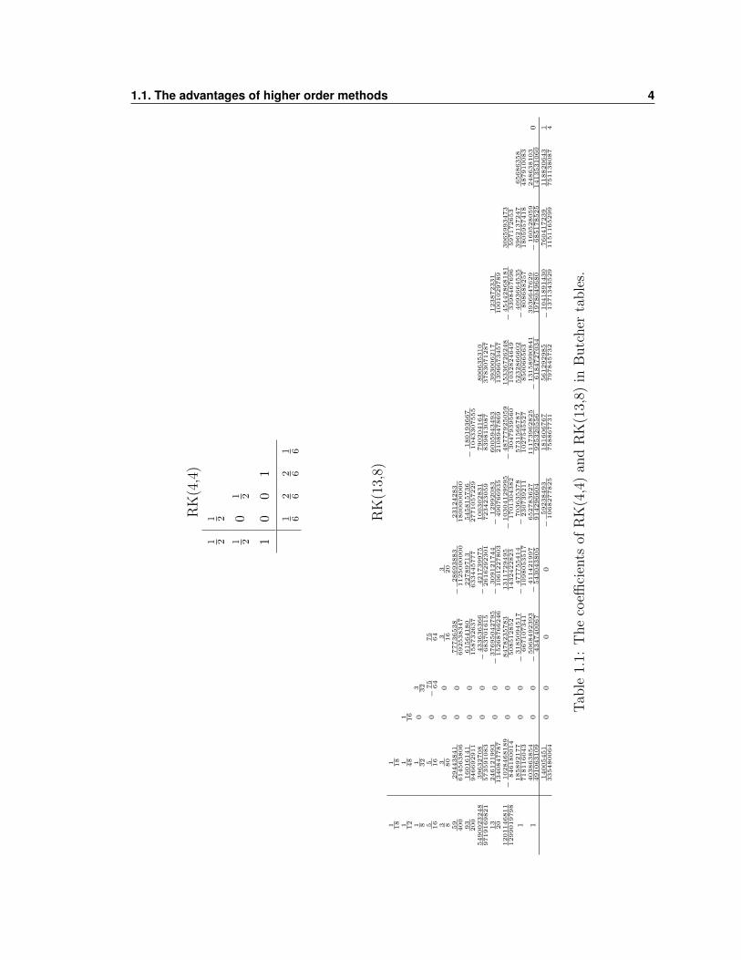
1.1 The coefficients of RK(4,4) and RK(13,8) in Butcher tables. . . . . . 4
2.1 Values of r(t), σ(t), γ(t) and α(t) of trees up to order 4 . . . . . . . 18
3.1 Cardinality of trees of order p and the number of order conditions. . 38
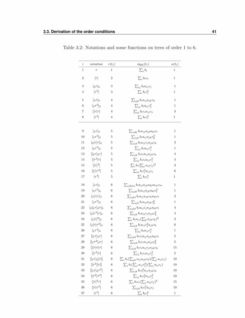
3.2 Notations and some functions on trees of order 1 to 6. . . . . . . . . 41
3.3 Notations and some functions on the remaining trees after applying
the simplifying conditions (3.3.29) for k = 0, 1. . . . . . . . . . . . . 42
3.4 Notations and some functions on the remaining trees after applying
the simplifying conditions (3.3.29) for k = 0, 1, 2. . . . . . . . . . . . 43
3.5 The contractivity preserving coefficients ccp and the interval of absolute
stability (α, 0) of CPHBTRK4(d, s, p) compared to T(p). . . . . . . . . . 55
4.1 The mean, median and standard deviation of the absolute value
of the difference |MGE − TOL| of CPHBTRK4(9, 6, 12) and T(12)
for the Henon Heiles, Equatorial main problem, the 20 DETEST
problems A,B,D,E and Kepler’s two body problem with eccentricity
ε = 0.99. . . . . . . . . . . . . . . . . . . . . . . . . . . . . . . . . . 64
4.2 The maximum global energy error (MGEE) and the number of steps
(NS) for CPHBTRK4(9, 6, 12) compared to T(12) and T(12)L for the
listed problems. . . . . . . . . . . . . . . . . . . . . . . . . . . . . . 65
xiii
LIST OF TABLES xiv
4.3 The NS PEG of CPHBTRK4(9, 6, 12) over T(12) for the listed prob-
lems. . . . . . . . . . . . . . . . . . . . . . . . . . . . . . . . . . . . 68
4.4 The NFE PEG of CPHBTRK4(9, 6, 12) over T(12) for the listed prob-
lems. . . . . . . . . . . . . . . . . . . . . . . . . . . . . . . . . . . . 69
4.5 The NS PEG and NFE PEG of CPHBTRK4(9, 6, 12) over T(12)L for
the listed problems. . . . . . . . . . . . . . . . . . . . . . . . . . . . 69
4.6 The CPU PEG of CPHBTRK4(9, 6, 12) over T(12) and DP(8,7)13M
for the listed problems. . . . . . . . . . . . . . . . . . . . . . . . . . 75
4.7 The CPU time in seconds, MGE, MGEE and NS of CPHBTRK4(9, 6, 12)
and T(12) for the DETEST class D problems and the Kepler prob-
lem with ε = 0.99. . . . . . . . . . . . . . . . . . . . . . . . . . . . . 76
4.8 The CPU time in seconds, MGE and NS of CPHBTRK4(9, 6, 12)
and T(12) for the Arenstorf problem, B1, B5, E2 and the Galactic
dynamics problems. . . . . . . . . . . . . . . . . . . . . . . . . . . . 77
5.1 The contractivity preserving coefficient ccp and the interval of absolute
stability (α, 0) of CPHBTRK5(d, s, p) compared to T(p). . . . . . . . . . 89
6.1 The maximum global energy error (MGEE) and the number of steps
(NS) for CPHBTRK5(8, 8, 12) compared to T(12) and T(12)L for the
listed problems. . . . . . . . . . . . . . . . . . . . . . . . . . . . . . . 96
6.2 The NS PEG and NFE PEG of CPHBTRK5(8, 8, 12) over T(12) for
the listed problems. . . . . . . . . . . . . . . . . . . . . . . . . . . . 97
6.3 The NS PEG and NFE PEG of CPHBTRK5(8, 8, 12) method over
T(12)L method for the listed problems. . . . . . . . . . . . . . . . . 99
6.4 The CPU PEG of CPHBTRK5(8, 8, 12) method over T(12), DP(8,7)13M
and CPHBTRK4(9, 6, 12) methods for the listed problems. . . . . . . 103
LIST OF TABLES xv
6.5 The CPU time in seconds, MGE, MGEE and NS of CPHBTRK5(8, 8, 12)
and T(12) for the DETEST class D problems and the Kepler prob-
lem with ε = 0.99. . . . . . . . . . . . . . . . . . . . . . . . . . . . . 104
6.6 The CPU time in seconds, MGE and NS of CPHBTRK5(8, 8, 12)
and T(12) for the Arenstorf problem, B1, B5, E2 and the Galactic
dynamics problems. . . . . . . . . . . . . . . . . . . . . . . . . . . . 105
Chapter 1
Introduction
Differential equations can be traced back to Isaac Newton [39] when he investigated
the solution of the differential equation [22]
dy
dx= 1− 3x+ y + x2 + xy (1.0.1)
and obtained a solution recursively as an infinite series. Since then, enormous ef-
forts were directed towards solving differential equations arising in different fields
such as chemistry, physics, biology, astronomy and weather/climate prediction. How-
ever, only a small percentage of the differential equations in the literature can be
solved analytically. Hence, numerical methods play a vital role in obtaining accurate
approximations to the exact solution of differential equations.
Huge efforts were directed towards developing, implementing and analyzing var-
ious numerical methods satisfying different accuracy and stability properties. In this
thesis, we establish a new class of high order, explicit, one-step, multi-stage, multi-
derivative, Hermite-Birkhoff-Taylor time discretizations satisfying certain stability
properties, in particular, the contractivity preserving property. These methods are
denoted by CPHBT.
1
1.1. The advantages of higher order methods 2
1.1 The advantages of higher order methods
In general, high order methods generate numerical solutions with higher accuracy
compared to lower order methods. However, in applications, the required accuracy
of the numerical solution is usually known and it is in general not extremely high.
Then, why do we search and derive higher order methods? There are at least two
good reasons:
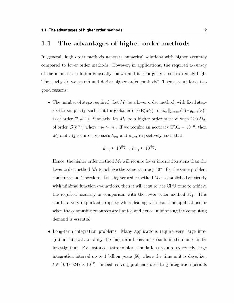
• The number of steps required: Let M1 be a lower order method, with fixed step-
size for simplicity, such that the global error GE(M1)=maxx ‖yexact(x)−ynum(x)‖
is of order O(hm1). Similarly, let M2 be a higher order method with GE(M2)
of order O(hm2) where m2 > m1. If we require an accuracy TOL = 10−n, then
M1 and M2 require step sizes hm1 and hm2 , respectively, such that
hm1 ≈ 10−nm1 < hm2 ≈ 10
−nm2 .
Hence, the higher order method M2 will require fewer integration steps than the
lower order method M1 to achieve the same accuracy 10−n for the same problem
configuration. Therefore, if the higher order method M2 is established efficiently
with minimal function evaluations, then it will require less CPU time to achieve
the required accuracy in comparison with the lower order method M1. This
can be a very important property when dealing with real time applications or
when the computing resources are limited and hence, minimizing the computing
demand is essential.
• Long-term integration problems: Many applications require very large inte-
gration intervals to study the long-term behaviour/results of the model under
investigation. For instance, astronomical simulations require extremely large
integration interval up to 1 billion years [50] where the time unit is days, i.e.,
t ∈ [0, 3.65242 × 10¹¹]. Indeed, solving problems over long integration periods
1.1. The advantages of higher order methods 3
will result in losing accuracy due to the propagation of discretization errors. As
an example, consider the modified oscillatory initial value problem [27]
y′ = 2y cos(x) y(0) = 1, (1.1.1)
with exact solution y(x) = e2 sin(x). We solved problem (1.1.1) using a 4-stage
Runge-Kutta method of order 4, RK(4,4), and a 13-stage Runge-Kutta method
of order 8, RK(13,8), with coefficients given in Table (1.1). We choose fixed
step sizes such that both methods use the same number of function evaluations.
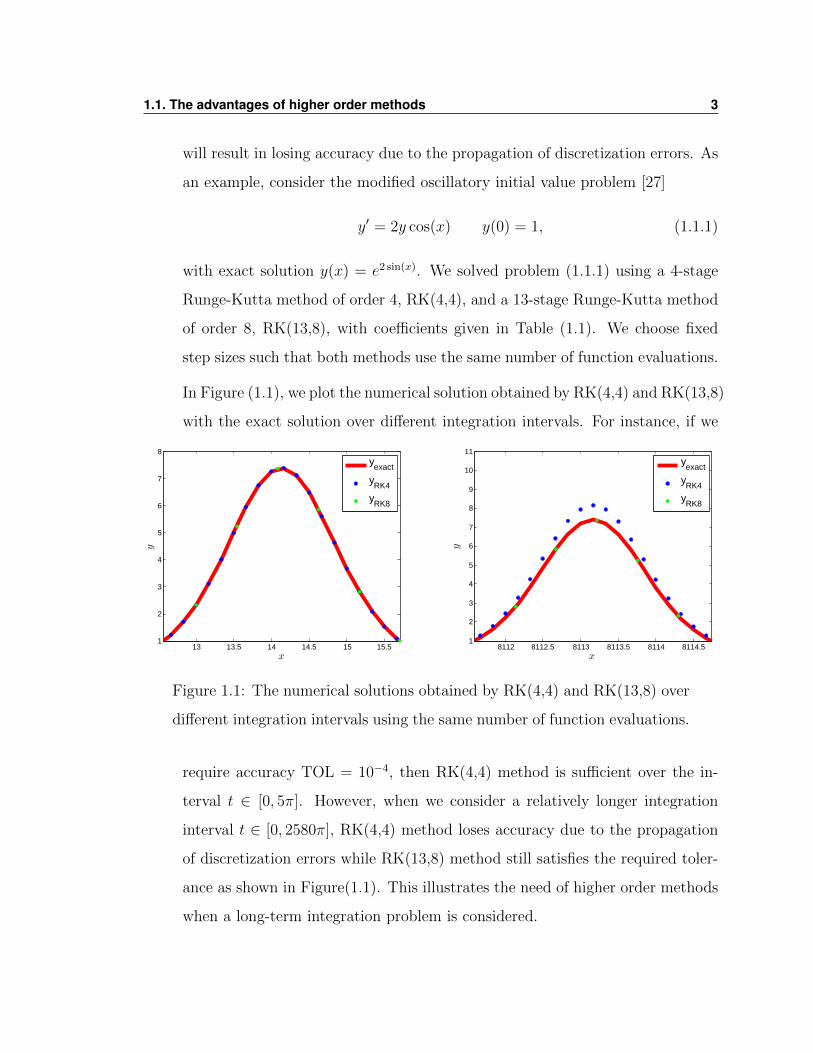
In Figure (1.1), we plot the numerical solution obtained by RK(4,4) and RK(13,8)
with the exact solution over different integration intervals. For instance, if we
13 13.5 14 14.5 15 15.51
2
3
4
5
6
7
8
x
y
8112 8112.5 8113 8113.5 8114 8114.51
2
3
4
5
6
7
8
9
10
11
x
y
y
exact
yRK4
yRK8
yexact
yRK4
yRK8
Figure 1.1: The numerical solutions obtained by RK(4,4) and RK(13,8) over
different integration intervals using the same number of function evaluations.
require accuracy TOL = 10−4, then RK(4,4) method is sufficient over the in-
terval t ∈ [0, 5π]. However, when we consider a relatively longer integration
interval t ∈ [0, 2580π], RK(4,4) method loses accuracy due to the propagation
of discretization errors while RK(13,8) method still satisfies the required toler-
ance as shown in Figure(1.1). This illustrates the need of higher order methods
when a long-term integration problem is considered.
1.1. The advantages of higher order methods 4
RK
(4,4
)1 2
1 2
1 20
1 2
10
01
1 62 6
2 61 6
RK
(13,
8)1 18
1 18
1 12
1 48
1 16
1 81 32
03 32
5 16
5 16
0−
75
64
75
64
3 83 80
00
3 16
3 20
59
400
29443841
614563806
00
77736538
692538347
−28693883
1125000000
23124283
1800000000
93
200
16016141
946692911
00
61564180
158732637
22789713
633445777
545815736
2771057229
−180193667
1043307555
5490023248
9719169821
39632708
573591083
00
−433636366
683701615
−421739975
2616292301
100302831
723423059
790204164
839813087
800635310
3783071287
13
20
246121993
1340847787
00
−37695042795
15268766246
−309121744
1061227803
−12992083
490766935
6005943493
2108947869
393006217
1396673457
123872331
1001029789
1201146811
1299019798
−1028468189
846180014
00
8478235783
508512852
1311729495
1432422823
−10304129995
1701304382
−48777925059
3047939560
15336726248
1032824649
−45442868181
3398467696
3065993473
597172653
1185892177
718116043
00
−3185094517
667107341
−477755414
1098053517
−703635378
230739211
5731566787
1027545527
5232866602
850066563
−4093664535
808688257
3962137247
1805957418
65686358
487910083
1403863854
491063109
00
−5068492393
434740067
−411421997
543043805
652783627
914296604
11173962825
925320556
−13158990841
6184727034
3936647629
1978049680
−160528059
685178525
248638103
1413531060
0
14005451
335480064
00
00
−59238493
1068277825
181606767
758867731
561292985
797845732
−1041891430
1371343529
760417239
1151165299
118820643
751138087
1 4
Tab
le1.
1:T
he
coeffi
cien
tsof
RK
(4,4
)an
dR
K(1
3,8)
inB
utc
her
table
s.
1.2. Contractivity preserving methods 5
1.2 Contractivity preserving methods
In 1988, Shu in [52] and Shu and Osher in [53] established strong stability preserving
Runge-Kutta methods, denoted by SSPRK. The derivation of such methods was
motivated by the observation that the solution of some partial differential equations
of the form
ux = Φ(x, u, uy, uyy, . . .) (1.2.1)
such as hyperbolic conservation laws, satisfies the monotonicity property
‖u(x+ ∆x)‖ ≤ ‖u(x)‖, (1.2.2)
where ‖ ·‖ is some norm such as the total variation norm [21, 52, 53]. Strong stability
preserving high order time discretization methods are designed for the time evolution
of hyperbolic partial differential equations with discontinuous solutions satisfying a
discrete form of inequality (1.2.2) as follows:
‖un+1‖ ≤ ‖un‖, (1.2.3)
where un, un+1 are numerical approximations of u(xn) and u(xn + ∆x), respectively.
Assuming that the SSP property (1.2.3) holds for the forward Euler method
un+1 = un + ∆xFEf(xn, un), (1.2.4)
Shu and Osher show that the SSP property (1.2.3) holds for the designed SSPRK
methods by expressing them as convex combination of the forward Euler method
with a modified step size, ∆x ≤ c∆xFE, where c is called the SSP coefficient. Since
then, significant efforts were directed towards deriving and optimizing SSP methods
[52, 53, 20, 17, 28, 45, 47, 46, 55]. The designed SSP methods were shown to be
more stable and suppressed the spurious oscillations and overshoot that may occur at
discontinuities in comparison with other non-SSP methods as shown by Gottlieb and
Shu in [20]. Also, most SSP methods have the same form and the same computational
cost as traditional ODE solvers.
1.2. Contractivity preserving methods 6
In this thesis, we are interested in the solution of non-stiff initial value problems
of the form:dy
dx= f(x, y(x)), y(x0) = y0, (1.2.5)
where f : R×RN → RN . The exact solution of some IVP of the form (1.2.5) naturally
preserve the contractivity property
‖y(x+ ∆x)− y(x+ ∆x)‖ ≤ ‖y(x)− y(x)‖, (1.2.6)
where y(x) and y(x) are two solutions with different neighbouring initial conditions
y(x0) and y(x0), respectively. Throughout this work, we assume that f is a sufficiently
smooth function such that for each x0 ∈ R and y0 = y(x0) ∈ RN , problem (1.2.5) has
a unique solution y : [x0,∞) → RN . Also, we suppose that there exists a norm ‖ · ‖
on RN such that inequality (1.2.6) holds. Under these assumptions, the initial value
problem (1.2.5) is said to be dissipative [31].
Hence, when we design a numerical method, we require that the numerical solu-
tion of the IVP (1.2.5) satisfies a discrete form of the contractivity preserving property
(1.2.6) as follows:
‖yn+1 − yn+1‖ ≤ ‖yn − yn‖, (1.2.7)
where yn and yn are two numerical solutions with different neighbouring initial condi-
tions y0 = y(x0) and y0 = y(x0), respectively. Moreover, the contractivity preserving
property (1.2.7) is a desired property to reduce the effect of the propagation of dis-
cretization errors. Since all numerical methods introduce discretization errors, one
can consider the introduction of such errors to the numerical solution as jumping from
one solution ynNendn=0 to another neighbouring perturbed solution ynNend
n=0 . Then, the
contractivity preserving property (1.2.7) will guarantee that the perturbed numerical
solution ynNendn=0 by the discretization errors will not ”wander away” from the exact
solution, i.e., it will minimize the effect of the propagation of the discretization errors
[33]. Kraaijevanger investigated in [31] the contractivity preserving Runge-Kutta
methods and established the necessary and sufficient conditions for Runge-Kutta
1.2. Contractivity preserving methods 7
methods to be contractive. However, the designed contractive Runge-Kutta methods
achieved limited order of accuracy with order barrier equals to 6 (p ≤ 6) for implicit
contractive Runge-Kutta methods. This order barrier is even more severe for explicit
contractive Runge-Kutta methods (p ≤ 4) [31, page 516]. One of the goals of this
work is to overcome this order barrier by casting Runge-Kutta methods with the
Taylor series method.
The Taylor series method is a successful classical method that has been inves-
tigated extensively. It has been shown that it is a competitive candidate in astro-
nomical simulations [3], solving general problems [8, 29, 34], sensitivity analysis of
ODEs/DAEs [2] and validating solutions of ODEs [38, 25]. The main computational
cost in solving ODEs by the Taylor method in terms of function evaluations and CPU
time lies in the repeated evaluation of the Taylor coefficients of the functions involved.
In [11], Deprit and Zahar showed that recursive computation of Taylor coefficients is
very effective in achieving high accuracy with little computing time and large step
sizes. Hence, the addition of higher order derivatives to Runge-Kutta methods can
be implemented efficiently using the notion of automatic differentiation [34]. In 2013,
Nguyen-Ba et al. [40], extended the forward Euler method used by Shu in [52] and
Shu and Osher in [53], to the expanded 9-derivative series:
yn+1 = yn + ∆xf(xn, yn) +9∑
m=2
ηm∆xmf (m−1)(xn, yn), (1.2.8)
and designed a two-step, contractivity preserving, explicit, 9-derivative, Hermite-
Obrechkoff method of order 13, denoted by HO(13), by expressing the method as a
convex combination of the expanded 9-derivative series (1.2.8). The designed 2-steps,
contractivity preserving (CP) HO(13) method has a larger region of absolute stability
compared to the Taylor method of order 13, T(13). Also, it reduces the number
of high order derivatives required by 4 compared to T(13) and hence it requires
less CPU time to achieve the same accuracy. Moreover, the CP HO(13) method is
successful in suppressing the error growth in long-term integration of Kepler’s two-
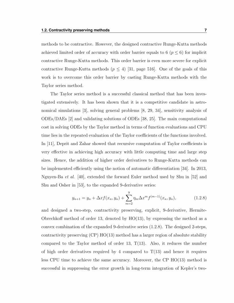
1.2. Contractivity preserving methods 8
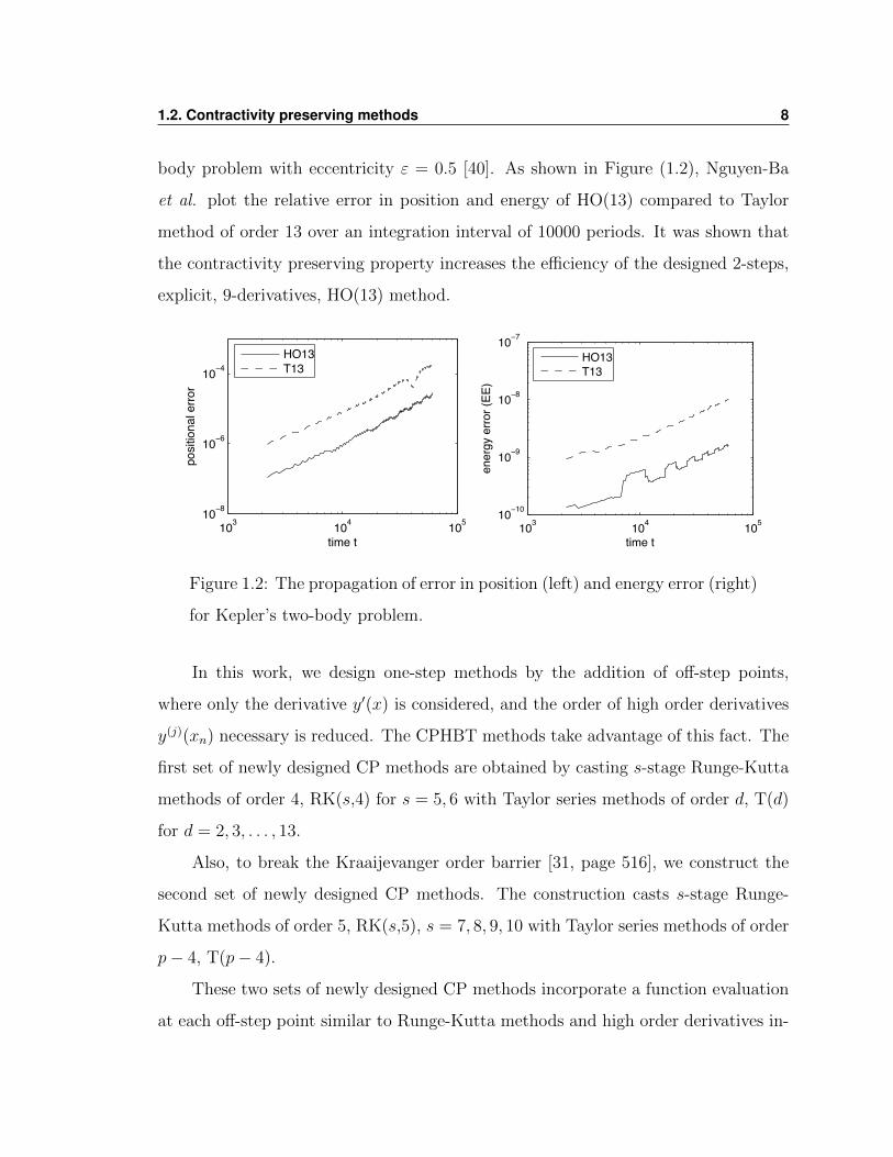
body problem with eccentricity ε = 0.5 [40]. As shown in Figure (1.2), Nguyen-Ba
et al. plot the relative error in position and energy of HO(13) compared to Taylor
method of order 13 over an integration interval of 10000 periods. It was shown that
the contractivity preserving property increases the efficiency of the designed 2-steps,
explicit, 9-derivatives, HO(13) method.
103 104 10510−8
10−6
10−4
time t
posit
iona
l erro
r
HO13T13
103 104 10510−10
10−9
10−8
10−7
time t
ener
gy e
rror (
EE)
HO13T13
Figure 1.2: The propagation of error in position (left) and energy error (right)
for Kepler’s two-body problem.
In this work, we design one-step methods by the addition of off-step points,
where only the derivative y′(x) is considered, and the order of high order derivatives
y(j)(xn) necessary is reduced. The CPHBT methods take advantage of this fact. The
first set of newly designed CP methods are obtained by casting s-stage Runge-Kutta
methods of order 4, RK(s,4) for s = 5, 6 with Taylor series methods of order d, T(d)
for d = 2, 3, . . . , 13.
Also, to break the Kraaijevanger order barrier [31, page 516], we construct the
second set of newly designed CP methods. The construction casts s-stage Runge-
Kutta methods of order 5, RK(s,5), s = 7, 8, 9, 10 with Taylor series methods of order
p− 4, T(p− 4).
These two sets of newly designed CP methods incorporate a function evaluation
at each off-step point similar to Runge-Kutta methods and high order derivatives in-
1.3. Thesis outline 9
formation as in Taylor series methods to achieve better performance than widely used
methods existing in the literature including Runge-Kutta and Taylor series methods.
Moreover, the designed methods overcome the order barriers of CP RK methods and
require significantly less high order derivatives compared to the Taylor series meth-
ods of the same order. In addition, a variable step algorithm with error estimation
formula is used to minimize the number of function evaluations required to achieve
the user defined tolerance, TOL, and to optimize the performance of CPHBT(d, s, p).
To test and analyze the performance of the designed methods, we consider more
than 30 test problems consisting of single equations, small systems, orbit equations,
higher order equations and Hamiltonian problems using C++, Fortran and MATLAB
codes. We show that the designed CPHBT(d, s, p) methods require significantly less
step points, less function evaluations and less CPU time to achieve the user defined
tolerance compared to well known, widely used ODEs solvers such as the Dormand-
Prince Runge Kutta pair DP(8,7)13M [43], Taylor series methods of order p, T(p),
and the Taylor method introduced by Martin Lara, T(p)L [34]. The designed meth-
ods have significantly larger regions of absolute stability compared to other methods
of the same order. Also, the contractivity preserving property minimizes the growth
of discretization errors when long-term integration problems are considered. These
results make our methods competitive candidates for astronomical computations [3].
1.3 Thesis outline
This chapter included a brief introduction and the motivation together with the con-
tributions of this work. The rest of the thesis can be outlined as follows:
In Chapter 2, we include a brief background of the theory and the definitions to
make this work self contained. We also discuss and describe the Runge-Kutta meth-
ods, Taylor methods, automatic differentiation and we list the DETEST problems
[27] used in this work.
1.4. Contributions 10
In Chapter 3, we present an introduction to the newly designed methods and
a detailed derivation of the order conditions of CPHBTRK4 methods by means of
rooted trees, B-series, elementary differentials and elementary weights. Moreover, we
formulate and prove the contractivity preserving property and represent the CPHBT
methods in different forms to facilitate and simplify the optimization problem. Fi-
nally, we formulate the optimization problem and we construct 24 new CPHBTRK4
methods.
In Chapter 4, we test, investigate and compare the newly designed methods
to other well known methods to show the efficiency, accuracy and stability of the
designed CPHBT methods. We also study the propagation of discretization errors of
the CPHBT methods when applied to a long-term integration problem.
In Chapter 5, we present the second set of methods, CPHBTRK5, and we derive
the order conditions and formulate the optimization process. Also, we study the
gain in the contractivity preserving coefficients, ccp, by analyzing the efficient CP
coefficient, ceffcp, compared to CPHBTRK4 presented in Chapter 4.
In Chapter 6, we present some numerical simulations and results by comparing
CPHBTRK5 to other methods including CPHBTRK4. We also study the propagation
of discretization errors compared to other methods including CPHBTRK4 and a well-
known, well tested Runge-Kutta-Nystrom pair designed by Philip Sharp in 2013 [49].
Finally, in Appendices A and B, we list the coefficients of 24 CPHBTRK4 methods
constructed in Chapter 3 and of 27 CPHBTRK5 methods constructed in Chapter 5,
respectively.
1.4 Contributions
In this section, we list the contributions of this thesis. We investigate and test our
results rigorously and we are hoping that these results will be a great addition to the
field of ODE solvers in general and to the contractivity preserving time discretization
1.4. Contributions 11
field in particular. Our main contribution is the derivation of two sets of new one-
step, explicit, multi-stage, multi-derivatives, contractivity preserving, HBT methods.
More precisely, our contributions can be summarized as follows:
1. We present the formulae of the new variable step, explicit, s-stage, d-derivative,
one-step, contractivity preserving Hermite-Birkhoff-Taylor methods in different
forms such as the Butcher form, the Shu-Osher form and the Canonical Shu-
Osher form in a compact vector notation.
2. We formulate the contractivity preserving property of CPHBT(d, s, p) presented
in two theorems utilizing the properties of a modified version of the Canonical
Shu-Osher form.
3. We derive the order condition of CPHBTRK4(d, s, p) and CPHBTRK5 (d, s, p)
methods of orders p = 5, 6, . . . , 15. Also, establishing the elementary weights
of the whole class of CPHBT that can be used recursively to obtain the order
conditions of any CPHBT method by means of rooted trees, B-series, elementary
weights and elementary differentials.
4. We formulate the nonlinear optimization problem and obtaining the nonnegative
coefficients (A, b,γ0) of 23 new optimal CPHBTRK4(d, s, p) methods for d =
2, 3, . . . , 13, p = 5, 6, . . . , 15 and s = 5, 6.
5. We formulate the nonlinear optimization problem and obtaining the nonnegative
coefficients (A, b,γ0) of 26 new optimal CPHBTRK5(d, s, p) methods for d =
2, 3, . . . , 10, p = 6, 7, . . . , 14 and s = 7, 8, 9, 10.
6. We study the performance of the two new sets of methods, CPHBTRK4 and
CPHBTRK5, compared to well known and widely used methods applied to more
than 30 test problems by:
1.4. Contributions 12
(a) Showing that, in general, the designed methods have large regions of abso-
lute stability and a fairly good percentage efficiency gain (PEG) in terms
of the number of steps, number of function evaluations and CPU time
compared to other well known methods of the same order.
(b) Analyzing the maximum global error (MGE) and the maximum global
energy error (MGEE) for various test problems.
(c) Testing the performance of the variable step algorithm by considering the
mean, median and standard deviation of the difference |MGE − TOL| of
21 different test problems over a range of user defined tolerances.
(d) Analyzing the contractivity preserving coefficients percentage efficiency
gain (ccp PEG) and the effective contractivity preserving coefficient, ceffcp.
(e) Investigating and analyzing the propagation of discretization errors of the
numerical solution in long-term integration of a standard N-body problem
(interval lengths of up to 800,000 periods).
Chapter 2
Preliminary background and
notations
In this chapter we will introduce briefly the background material used in this thesis.
We will follow the notations and work presented in [18, 22, 30, 33].
2.1 Runge-Kutta methods
2.1.1 Formulation and classification
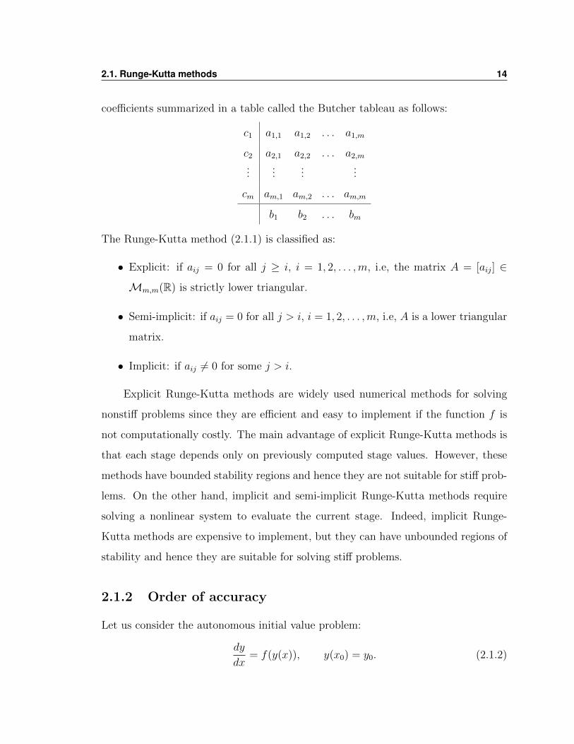
An s-stage Runge-Kutta method is written in the Butcher form as follows:
Yi = yn + ∆xs∑j=1
aijFj, i = 1, 2, . . . , s,
yn+1 = yn + ∆xs∑j=1
bjFj, (2.1.1)
where aij, bj and cj are the Runge-Kutta coefficients, yn+1 is an approximation of
y(xn+1), Yj is the stage value and Fj = f (xn + ∆xcj, Yj) is the stage derivative for
j = 1, 2, . . . , s. In the literature, Runge-Kutta methods are represented by their
13
2.1. Runge-Kutta methods 14
coefficients summarized in a table called the Butcher tableau as follows:
c1 a1,1 a1,2 . . . a1,m
c2 a2,1 a2,2 . . . a2,m
......
......
cm am,1 am,2 . . . am,m
b1 b2 . . . bm
The Runge-Kutta method (2.1.1) is classified as:
• Explicit: if aij = 0 for all j ≥ i, i = 1, 2, . . . ,m, i.e, the matrix A = [aij] ∈
Mm,m(R) is strictly lower triangular.
• Semi-implicit: if aij = 0 for all j > i, i = 1, 2, . . . ,m, i.e, A is a lower triangular
matrix.
• Implicit: if aij 6= 0 for some j > i.
Explicit Runge-Kutta methods are widely used numerical methods for solving
nonstiff problems since they are efficient and easy to implement if the function f is
not computationally costly. The main advantage of explicit Runge-Kutta methods is
that each stage depends only on previously computed stage values. However, these
methods have bounded stability regions and hence they are not suitable for stiff prob-
lems. On the other hand, implicit and semi-implicit Runge-Kutta methods require
solving a nonlinear system to evaluate the current stage. Indeed, implicit Runge-
Kutta methods are expensive to implement, but they can have unbounded regions of
stability and hence they are suitable for solving stiff problems.
2.1.2 Order of accuracy
Let us consider the autonomous initial value problem:
dy
dx= f(y(x)), y(x0) = y0. (2.1.2)
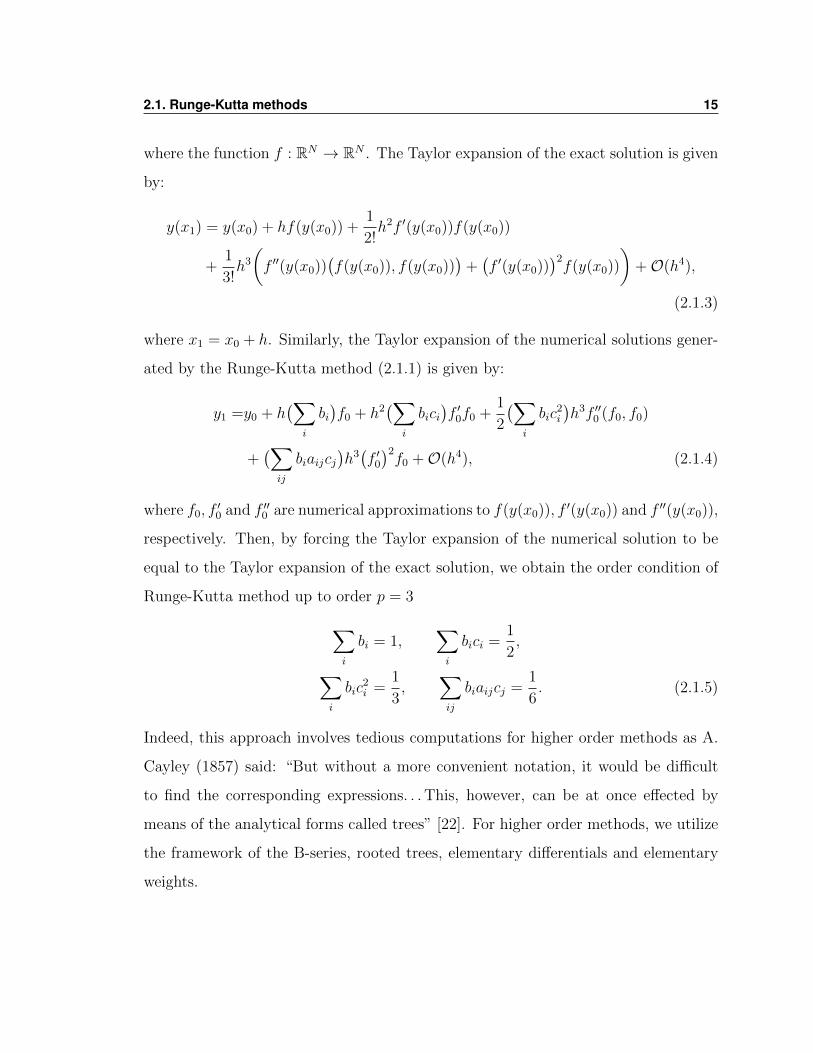
2.1. Runge-Kutta methods 15
where the function f : RN → RN . The Taylor expansion of the exact solution is given
by:
y(x1) = y(x0) + hf(y(x0)) +1
2!h2f ′(y(x0))f(y(x0))
+1
3!h3
(f ′′(y(x0))
(f(y(x0)), f(y(x0))
)+(f ′(y(x0))
)2f(y(x0))
)+O(h4),
(2.1.3)
where x1 = x0 + h. Similarly, the Taylor expansion of the numerical solutions gener-
ated by the Runge-Kutta method (2.1.1) is given by:
y1 =y0 + h(∑
i
bi)f0 + h2
(∑i
bici)f ′0f0 +
1
2
(∑i
bic2i
)h3f ′′0 (f0, f0)
+(∑ij
biaijcj)h3(f ′0)2f0 +O(h4), (2.1.4)
where f0, f′0 and f ′′0 are numerical approximations to f(y(x0)), f ′(y(x0)) and f ′′(y(x0)),
respectively. Then, by forcing the Taylor expansion of the numerical solution to be
equal to the Taylor expansion of the exact solution, we obtain the order condition of
Runge-Kutta method up to order p = 3∑i
bi = 1,∑i
bici =1
2,
∑i
bic2i =
1
3,
∑ij
biaijcj =1
6. (2.1.5)
Indeed, this approach involves tedious computations for higher order methods as A.
Cayley (1857) said: “But without a more convenient notation, it would be difficult
to find the corresponding expressions. . . This, however, can be at once effected by
means of the analytical forms called trees” [22]. For higher order methods, we utilize
the framework of the B-series, rooted trees, elementary differentials and elementary
weights.
2.1. Runge-Kutta methods 16
2.1.3 Rooted trees
The theory of rooted trees is a large branch of graph theory and it is out of the scope
of this thesis. We will just summarize the relevant definitions, topics and results, in
particular, the one-to-one correspondence between rooted trees and Taylor expansion
derivatives. For more details, we refer the reader to [7, 22, 36].
Definition 2.1.1 [33] A rooted tree is a pair of nodes (P, S) where S is a finite set
of “Sons” or “Edges” and P is a finite set of “Parents”, also known as “Vertices”,
such that:
• A tree t is a connected graph with one node in P considered as the root of the
tree which never appears as a son.
• Other than the root, every parent node appears only once as a son in the tree.
• The order of a tree t is the number of its nodes and denoted by r(t).
Notation 2.1.1 • T denotes the set of all rooted trees and Tk is the set of all
rooted trees of order k.
• τ denotes the unique tree of order 1.
• t = [t1t2 . . . tn] denotes the rooted tree generated by connecting the roots of
t1, t2, . . . , tn to one more parent which represents the root of the tree t. This
process is called grafting.
• If t = [t1t2 . . . tn], then t1, t2, . . . , tn are the rooted trees generated by removing
the root of the tree t.
• t = [t1n1t2
n2 . . . tknk ] is the rooted tree generated by grafting n1, n2, . . . , nk dupli-
cates of the trees t1, t2, . . . , tk, respectively.
2.1. Runge-Kutta methods 17
Definition 2.1.2 [33, page 164] Let t = [t1n1t2
n2 . . . tknk ], then the order r(t), the
symmetry σ(t) and the density γ(t) of a rooted tree t are defined by
r(τ) = σ(τ) = γ(τ) = 1
r(t) = 1 +k∑i=1
nir(ti),
σ(t) =k∏i=1
ni!σ(ti)ni ,
γ(t) = r(t)k∏i=1
γ(ti)ni .
Moreover, we define the number of essentially different ways of labelling a tree mono-
tonically by
α(t) =r(t)!
σ(t)γ(t). (2.1.6)
Table 2.1 presents the values of r(t), σ(t), γ(t) and α(t) of trees up to order 4 [33].
For more details, we refer to [22, page 147] and [33, page 165].
Notation 2.1.2 We denote n copies of a tree t1 by tn1 ,
[[[. . . [︸ ︷︷ ︸k-times
by [k and ]]] . . .]︸ ︷︷ ︸k-times
by ]k.
2.1.4 Elementary differentials and elementary weights
In this section, following Butcher’s book [6], we will introduce the elementary differ-
entials and elementary weights of Runge-Kutta methods. Recall that since f : RN →
RN , then its first derivative evaluated at y is a linear operator given by the matrix of
partial derivatives of f . Similarly, the m-th derivative of f , f (m)(y), is a multilinear
2.1. Runge-Kutta methods 18
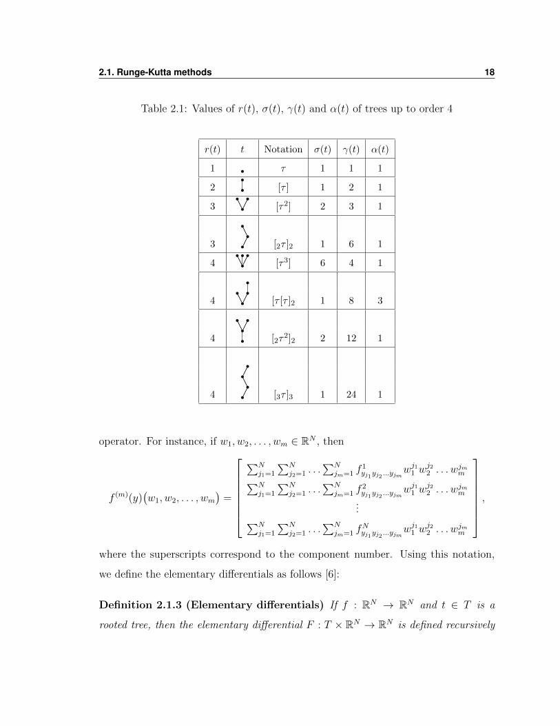
Table 2.1: Values of r(t), σ(t), γ(t) and α(t) of trees up to order 4
r(t) t Notation σ(t) γ(t) α(t)
1 r τ 1 1 1
2 rr [τ ] 1 2 1
3 rr rAA [τ2] 2 3 1
3 rr rAA [2τ ]2 1 6 1
4 rr rrAA [τ3] 6 4 1
4 rrrr
AA [τ [τ ]2 1 8 3
4 rrrrAA
[2τ2]2 2 12 1
4 r rr rAA
[3τ ]3 1 24 1
operator. For instance, if w1, w2, . . . , wm ∈ RN , then
f (m)(y)(w1, w2, . . . , wm
)=
∑Nj1=1
∑Nj2=1 . . .
∑Njm=1 f
1yj1yj2 ...yjm
wj11 wj22 . . . wjmm∑N
j1=1
∑Nj2=1 . . .
∑Njm=1 f
2yj1yj2 ...yjm
wj11 wj22 . . . wjmm
...∑Nj1=1
∑Nj2=1 . . .
∑Njm=1 f
Nyj1yj2 ...yjm
wj11 wj22 . . . wjmm
,
where the superscripts correspond to the component number. Using this notation,
we define the elementary differentials as follows [6]:
Definition 2.1.3 (Elementary differentials) If f : RN → RN and t ∈ T is a
rooted tree, then the elementary differential F : T × RN → RN is defined recursively
2.1. Runge-Kutta methods 19
as follows:
F (τ)(y) = f(y), (2.1.7)
F ([t1t2 . . . tm]) (y) = f (m)(y) (F (t1)(y), F (t2)(y), . . . , F (tm)(y)) . (2.1.8)
Rooted trees are particularly useful in expressing the derivatives of y(x) in terms of f
and its partial derivatives. This is neatly summed up by Butcher [7] in the following
theorem stating that the m-th derivative of y is a linear combination of all elementary
differentials of order m.
Theorem 2.1.1 If y′(x) = f(y(x)) where f : RN → RN . Then, the k-th derivative
of the exact solution y is given by
y(k) =∑t∈Tk
α(t)F (t)(y). (2.1.9)
Moreover, the quantities in equations (2.1.5) are called the elementary weights
of the Runge-Kutta method (2.1.1) and can be defined recursively as follows [33]:
Definition 2.1.4 (Elementary weights) The elementary weights of an s-stage Runge-
Kutta method corresponding to the rooted tree t = [t1t2 . . . tm] ∈ T , denoted by ΦRK(t),
is defined recursively by
Φi(τ) =s∑j=1
aij, (2.1.10)
Φi(t) =s∑j=1
aijΦi(t1)Φi(t2) . . .Φi(tm), (2.1.11)
ΦRK(t) =s∑i=1
biΦi(t1)Φi(t2) . . .Φi(tm). (2.1.12)
It is worth noting that different methods have different elementary weights. The
above definition is strictly for an s-stage Runge-Kutta method of the form (2.1.1).
2.1. Runge-Kutta methods 20
2.1.5 The B-series and the order conditions
The B-series is named after John Charles Butcher [7] in his elegant interpretation of
the Taylor expansions of the exact and the numerical solutions.
Definition 2.1.5 (B-series) Let a : T → R be a real valued function on T . Then,
a B-series is defined as follows:
B(a, y) =∑t∈T
hr(t)
r(t)!α(t)a(t)F (t)(y). (2.1.13)
We can rewrite the Taylor expansion of the exact solution in (2.1.3) as a B-series
as follows [6, page 155]:
Theorem 2.1.2 The Taylor expansion of the exact solution y1 = y(x0 + h) is equal
to
y(x1) = y(x0) +
p∑i=1
hi∑t∈Ti
1
σ(t)γ(t)F (t)(y(x0)) +O(hp+1). (2.1.14)
Similarly, by using the elementary weights (2.1.10)-(2.1.12), we can rewrite the Taylor
expansion of the numerical solution in (2.1.4) as a B-series as follows [6, page 160]:
Theorem 2.1.3 The Taylor expansion of the numerical solution of the Runge-Kutta
method is given by
y1 = y0 +
p∑i=1
hi∑t∈Ti
1
σ(t)ΦRK(t)F (t)(y0) +O(hp+1). (2.1.15)
Hence, by comparing equations (2.1.14) and (2.1.15), we get the following theo-
rem [33, page169]:
Theorem 2.1.4 The Runge-Kutta method has order p if and only if ΦRK(t) = 1γ(t)
holds for all rooted trees of order r(t) ≤ p and does not hold for some tree of order
p+ 1.
2.1. Runge-Kutta methods 21
Finally, we state a very important theorem for the derivation of the order condition
of higher order methods [22]:
Theorem 2.1.5 If a : T → R, a(φ) = 1 and t = [t1, t2, . . . , tm], then
hf(B(a, y)) = B(a′, y),
where a′(φ) = 0, a′(τ) = 1 and a′(t) = r(t)a(t1)a(t2) . . . a(tm).
2.1.6 Linear stability of Runge-Kutta methods
In this section, we consider the vector notation of the Runge-Kutta method (2.1.1)
operating on scalar problems as follows:
Y = eyn + hAF ,
yn+1 = yn + hbTF , (2.1.16)
where Y = [Y1, Y2, . . . , Ys]T ∈ Rs, F = [F1, F2, . . . , Fs]
T ∈ Rs, e = [1, 1, . . . , 1]T ∈ Rs,
A = (aij) ∈ Ms,s(R), and b = [b1, b2, . . . , bs]T ∈ Rs. Applying the Runge-Kutta
method (2.1.16) to the Dahlquist test equation [33, page 198]
y′ = λy, y(0) = 1, λ ∈ C,
we get the following:
Y = eyn + zAY ,
yn+1 = yn + zbTY , (2.1.17)
where z = λh. Solving the two equations simultaneously for yn+1 in terms of yn, we
obtain:
yn+1 =
[1 + zbT (I − zA)−1e
]yn, (2.1.18)
where R(z) = 1+zbT (I−zA)−1e is the stability function of the Runge-Kutta method
provided that (I − zA)−1 is invertible [33]. Moreover, Dekker and Verwer derived
2.2. Taylor series method 22
an alternative form of the stability function as a ratio of two determinants as follows
[18]:
R(z) =|I − zA+ zebT ||I − zA|
. (2.1.19)
Definition 2.1.1 The stability region is the set of all values of z in the complex plain
such that |R(z)| ≤ 1.
We note that for explicit Runge-Kutta methods, (I−zA) is a lower triangular matrix
and |I − zA| = 1. Then, by (2.1.19), the stability functions of explicit Runge-Kutta
methods are always polynomials and hence their regions of absolute stability are
finite. Indeed, for implicit Runge-Kutta methods, (I − zA) is a polynomial in z, so
the stability function (2.1.19) is a rational function in z and it is possible to have an
infinite region of absolute stability.
2.2 Taylor series method
Consider the non-autonomous initial value problem
y′(x) = f(x, y) y(x0) = y0, (2.2.1)
where f : [a, b]×RN → RN and y : [a, b]→ RN . The Taylor expansion of degree p of
y about xn evaluated at xn+1 is given by
y(xn+1) = y(xn) + hy(1)(xn) +h2
2!y(2)(xn) + . . .+
hp
p!y(p)(xn) +O(hp+1) (2.2.2)
where h = ∆x and
y(2) = fx + fyy′ = fx + fyf,
y(3) = fxx + 2fxyf + fyy(f, f) + fy(fx + fyf),
...
(2.2.3)
2.2. Taylor series method 23
The Taylor series method of order p, T(p), is equivalent to the truncated Taylor series
expansion of degree p of the exact solution in (2.2.2) and is given as follows:
yn+1 = yn + hy(1)n +
h2
2!y(2)n + . . .+
hp
p!y(p)n , (2.2.4)
where yn and yn+1 are approximations of y(xn) and y(xn+1), respectively. This method
is commonly used in many fields such as the astronomical computations field since it is
very successful in reaching high order accuracy. However, as we can see in (2.2.3), the
repeated computation of the Taylor coefficients Y [i] = 1i!y(i) and F [i] = 1
i!(f(x, y(x))(i)
of y(x) and f(x, y(x)), respectively, can be very costly for higher derivatives. So,
the Taylor coefficients are computed efficiently by an extension of Newton’s approach
which has been rediscovered several times (Steffensen 1956 [57]). Throughout this
work, we use the notation Y [i] = 1i!y(i) and F [i] = 1
i!(f(x, y(x))(i) to refer to the
normalized i-th derivative of y(x) and f(x, y(x)), respectively.
2.2.1 Automatic differentiation
The exact solution can be written in terms of its Taylor coefficients as follows:
y(t0 + h) =
p∑i=0
hi
i!y(i) +O(hp+1) =
p∑i=0
hiY [i] +O(hp+1).
Then, from (2.2.1),
Y [i+1] =1
i+ 1F [i]. (2.2.5)
Now suppose that f(x, y) is the composition of a finite sequence of algebraic operations
and elementary functions (multiplication, division, ln, sin, cos, . . .). This leads to
a finite sequence of series that forms f [22, page 46]. For each given series p =∑∞i=0 P
[i]hi, q =∑∞
i=0Q[i]hi, r =
∑∞i=0R
[i]hi, we can find formulae to generate the
i-th Taylor coefficient from the preceding ones as follows:
a) If r = p± q, then
R[i] = P [i] ±Q[i], i = 0, 1, . . . (2.2.6)
2.2. Taylor series method 24
b) If r = pq, then the Cauchy product yields
R[i] =i∑
j=0
P [j]Q[i−j], i = 0, 1, . . . (2.2.7)
c) If r = pq, q 6= 0, then by writing p = rq, using formula b) and solving for R[i],
we get:
R[i] =1
Q0
[P [i] −
i∑j=1
R[i−j]Q[j]
], i = 0, 1, . . . (2.2.8)
d) If r = pα, then
R[i] =1
iP0
i−1∑j=0
(iα− j(α + 1))P [i−j]R[j]. (2.2.9)
e) If r = ep, then
R[i] =1
i
i−1∑j=0
(i− j)R[j]P [i−j]. (2.2.10)
f) If r = ln(p), then
R[i] =1
P0
[P [i] − 1
i
i−1∑j=1
(i− j)P [j]R[i−j]]. (2.2.11)
g) If r = cos(p) and q = sin(p), then
R[i] =−1
i
i∑j=1
jQ[i−j]P [j], (2.2.12)
Q[i] =1
i
i∑j=1
jR[i−j]P [j]. (2.2.13)
There are formulae for several other elementary functions including inverse trigono-
metric functions. For more details and proves of the above formulas, refer to [37, 29,
34]
2.3. DETEST problems 25
2.3 DETEST problems
In this thesis, we consider a bank of test problems called DETEST for the purpose
of testing the designed contractivity preserving methods and comparing them to well
known, well tested ordinary differential equations solvers in the literature. This bank
of problems is accepted in the numerical ODE community as a standard compari-
son tool between higher order ODE solvers and has been used by several authors
[23, 41, 40, 51]. In our work, we utilize 20 of the DETEST problems of classes A, B,
D and E. We describe these classes briefly below [27]:
2.3.1 Problem class A: Single equations
• A1: The negative exponential.
y′ = −y, y(0) = 1. (solution: y = e−x)
• A2: A special case of the Riccati equation [10, page 73]:
y′ =−y3
2, y(0) = 1. (solution: y =
1√x+ 1
)
• A3: An oscillatory problem:
y′ = y cosx, y(0) = 1. (solution: y = esinx)
• A4: A logistic curve [10, page 97]:
y′ =y
4
(1− y
20
), y(0) = 1. (solution: y =
20
1 + 19e−x4
)
• A5: A spiral curve [10, page 38]:
y′ =y − xy + x
, y(0) = 4. (solution in polar coordinates: r = 4eπ2−θ)
2.3. DETEST problems 26
2.3.2 Problem class B: Small systems
• B1: The growth of two conflicting populations [10, page 102].
y′1 = 2(y1 − y1y2), y1(0) = 1,
y′2 = −(y2 − y1y2), y2(0) = 3.
• B2: A linear chemical reaction [16, page 175]:
y′1 = −y1 + y2, y1(0) = 2,
y′2 = y1 − 2y2 + y3, y2(0) = 0,
y′3 = y2 − y3, y3(0) = 1.
• B3: A nonlinear chemical reaction [16, page 177]:
y′1 = −y1, y1(0) = 1,
y′2 = y1 − y22, y2(0) = 0,
y′3 = y22, y3(0) = 0.
• B4: The integral surface of a torus [9, page 9]:
y′1 = −y2 −y1y3√y2
1 + y22
, y1(0) = 3,
y′2 = y1 −y2y3√y2
1 + y22
, y2(0) = 0,
y′3 =y1√y2
1 + y22
, y3(0) = 0.
• B5: The Euler equations of motion for a rigid body without external forces
[32]:
y′1 = y2y3, y1(0) = 0,
y′2 = −y1y3, y2(0) = 1,
y′3 = −0.51y1y2, y3(0) = 1.
2.3. DETEST problems 27
2.3.3 Problem class D: Orbit equations
• D1:
y′1 = y3, y1(0) = 1− ε,
y′2 = y4, y2(0) = 0,
y′3 =−y1
(y21 + y2
2)32
, y3(0) = 0,
y′4 =−y2
(y21 + y2
2)32
, y4(0) =
√1 + ε
1− ε,
where ε = 0.1 is the eccentricity of the orbit.
• D2: As above with ε = 0.3.
• D3: As above with ε = 0.5.
• D4: As above with ε = 0.7.
• D5: As above with ε = 0.9.
All the D class problems are derived from the orbit equations
x′′ =−xr3, x(0) = 1− ε, x′(0) = 0,
y′′ =−yr3, y(0) = 0, y′(0) =
√1 + ε
1− ε,
r2 = x2 + y2,
with solution
x = cosu− ε, x′ =− sinu
1− ε cosu,
y =√
1− ε2 sinu, y′ =
√1− ε2 cosu
1− ε cosu,
where u− ε sinu− t = 0.
2.3. DETEST problems 28
2.3.4 Problem class E: Higher order equations
• E1:
y′1 = y2, y1(0) = J 12(1) = 0.673967071418030,
y′2 = −(
y2
x+ 1+
(1− 0.25
(x+ 1)2
)y1
), y2(0) = J ′1
2(1) = 0.09540051444747446.
This is an ODE system derived from Bessel’s equation of order 1/2 with the
origin shifted one unit to the left [10, page 4,69]:
(x+ 1)2y′′ + (x+ 1)y′ + ((x+ 1)2 − 0.25)y = 0.
• E2:
y′1 = y2, y1(0) = 2,
y′2 = (1− y21)y2 − y1, y2(0) = 0.
This is an ODE system derived from the Van der Pol’s equation [10, page 358,
531]:
y′′ − (1− y2)y′ + y = 0.
• E3:
y′1 = y2, y1(0) = 0,
y′2 =y3
1
6− y1 + 2 sin (2.78535x), y2(0) = 0.
This is an ODE system derived from the Duffing’s equation [10, page 390]:
y′′ + y − y3
6= 2 sin (2.78535x).
• E4:
y′1 = y2, y1(0) = 30,
y′2 = 0.32− 0.4y22, y2(0) = 0.
2.3. DETEST problems 29
This is an ODE system derived from the falling body equation [10, page 60]:
y′′ = 0.32− 0.4y′2.
• E5:
y′1 = y2, y1(0) = 0,
y′2 =
√1 + y2
2
25− x, y2(0) = 0.
This is an ODE system derived from a linear pursuit equation [10, page 117]:
1 + (y′)2 = (25− x)2(y′′)2.
Chapter 3
CP s-Stage HBT methods based
on combining T(d) and RK(s,4)
methods
3.1 Introduction
In this chapter, we consider the solution of non-stiff autonomous initial value problem
of the formdy
dx= f(x, y(x)), y(x0) = y0, (3.1.1)
where the function f : R × RN → RN is a sufficiently smooth function. We present
the formulae of the new explicit contractivity preserving, one-step, s-stages, ex-
plicit, Hermite-Birkhoff-Taylor ODE solver of orders p = 5, 6, . . . , 15, denoted by
CPHBTRK4(d, s, p), with nonnegative coefficients by combining an s-stages Runge-
Kutta method of order 4, RK(s, 4), for s = 5, 6, with a Taylor series method, T(d), of
order d. The newly designed methods incorporate the function evaluations at off-step
points similar to Runge-Kutta methods and the high order derivatives information
as in Taylor series methods to achieve better performance than widely used methods
30
3.2. Formulation of CPHBTRK4(d, s, p) in Butcher form 31
existing in the literature including Runge-Kutta and Taylor series methods.
For the analysis of the new CPHBTRK4(d, s, p) methods, we define the forward
Euler expanded series, FES(d),
yn+1 = yn + ∆xf(xn, yn) +d∑
m=2
ηm∆xmf (m−1)(xn, yn). (3.1.2)
We are interested in the contractivity preserving property,
‖yn+1 − yn+1‖ ≤ ‖yn − yn‖, (3.1.3)
where yn, yn are two numerical solutions with different neighbouring initial conditions
y(x0) = y0, y(x0) = y0. Throughout this work, we assume that ‖ · ‖ is a norm such
that f is dissipative with respect to ‖·‖ [31]. To achieve inequality (3.1.3), we suppose
that there exists a step-size ∆FES(d) such that∥∥∥∥yn+1 − yn+1
∥∥∥∥ =
∥∥∥∥yn +d∑
m=1
ηm(∆x)mf (m−1)(xn, yn)
− yn −d∑
m=1
ηm(∆x)mf (m−1)(xn, yn)
∥∥∥∥≤ ‖yn − yn‖ (3.1.4)
holds for all ∆x ≤ ∆FES(d).
3.2 Formulation of CPHBTRK4(d, s, p) in Butcher
form
We call our new method CPHBTRK4(d, s, p) because we use Hermite-Birkhoff inter-
polation polynomials to define the predictors Pi and obtain the stages Yi to order
p− 3 as follows:
Yi = yn + ∆xi−1∑j=1
ai,jFj +d∑
m=2
(∆x)mγi,m y(m)n , i = 2, 3, . . . , s. (3.2.1)
3.2. Formulation of CPHBTRK4(d, s, p) in Butcher form 32
Also, we use Hermite-Birkhoff interpolation polynomials to define the integration
formula (IF) and obtain yn+1 to order p as follows:
yn+1 = yn + ∆xs∑j=1
bjFj +d∑
m=2
(∆x)mγs+1,m y(m)n , (3.2.2)
where in the formula of CPHBTRK4(d, s, p) we have the Runge-Kutta coefficients
ai,j, bj, cj for i = 2, 3, . . . , s, j = 1, 2, . . . , i − 1, and the Taylor coefficients γi,m for
i = 2, 3, . . . , s+1 and m = 2, 3, . . . , d. The high order derivatives y(m)n , m = 2, 3, . . . , d,
are evaluated only once per time step integration at the step point xn. Note that the
CPHBTRK4(d, s, p) formula (3.2.1)-(3.2.2) is given in the Butcher form. Following the
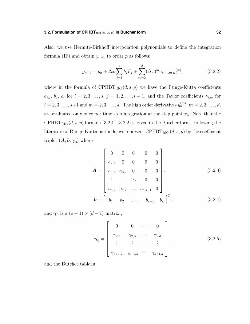
literature of Runge-Kutta methods, we represent CPHBTRK4(d, s, p) by the coefficient
triplet (A, b,γ0) where
A =
0 0 0 0 0
a2,1 0 0 0 0
a3,1 a3,2 0 0 0...
.... . . 0 0
as,1 as,2 . . . as,s−1 0
, (3.2.3)
b =[b1 b2 . . . bs−1 bs
]T, (3.2.4)
and γ0 is a (s+ 1)× (d− 1) matrix ,
γ0 =
0 0 · · · 0
γ2,2 γ2,3 · · · γ2,d
...... · · · ...
γs+1,2 γs+1,3 · · · γs+1,d
, (3.2.5)
and the Butcher tableau
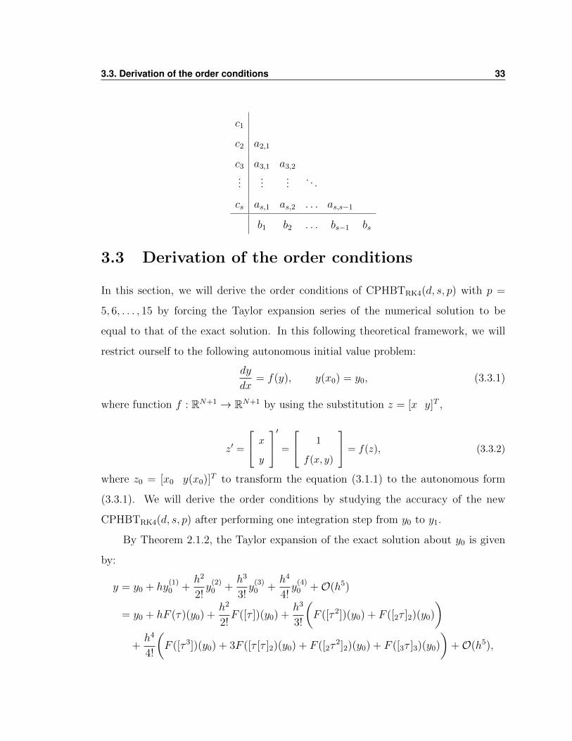
3.3. Derivation of the order conditions 33
c1
c2 a2,1
c3 a3,1 a3,2
......
.... . .
cs as,1 as,2 . . . as,s−1
b1 b2 . . . bs−1 bs
3.3 Derivation of the order conditions
In this section, we will derive the order conditions of CPHBTRK4(d, s, p) with p =
5, 6, . . . , 15 by forcing the Taylor expansion series of the numerical solution to be
equal to that of the exact solution. In this following theoretical framework, we will
restrict ourself to the following autonomous initial value problem:
dy
dx= f(y), y(x0) = y0, (3.3.1)
where function f : RN+1 → RN+1 by using the substitution z = [x y]T ,
z′ =
x
y
′ = 1
f(x, y)
= f(z), (3.3.2)
where z0 = [x0 y(x0)]T to transform the equation (3.1.1) to the autonomous form
(3.3.1). We will derive the order conditions by studying the accuracy of the new
CPHBTRK4(d, s, p) after performing one integration step from y0 to y1.
By Theorem 2.1.2, the Taylor expansion of the exact solution about y0 is given
by:
y = y0 + hy(1)0 +
h2
2!y
(2)0 +
h3
3!y
(3)0 +
h4
4!y
(4)0 +O(h5)
= y0 + hF (τ)(y0) +h2
2!F ([τ ])(y0) +
h3
3!
(F ([τ 2])(y0) + F ([2τ ]2)(y0)
)+h4
4!
(F ([τ 3])(y0) + 3F ([τ [τ ]2)(y0) + F ([2τ
2]2)(y0) + F ([3τ ]3)(y0)
)+O(h5),
3.3. Derivation of the order conditions 34
where h = ∆x and F (τ)(y0), F ([τ ])(y0), . . . , F ([3τ ]3)(y0) are elementary differentials
corresponding to the rooted trees τ, [τ ], . . . , [3τ ]3, respectively, as discussed briefly
in Section 2.1.4 and the subscript in [n and ]n . For more details, we refer to [22].
We utilize the framework of B-series with the elementary differentials, elementary
weights and rooted trees to express the Taylor series expansion of the exact solution
and the numerical solution as B-series and compare the coefficient sequences, also
called elementary weights, to derive the order conditions.
Theorem 3.3.1 The elementary weights Ψ : T → R of an s-stage, d-derivative
CPHBT method (3.2.1)-(3.2.2) corresponding to the rooted tree t = [t1 t2 . . . tn] ∈ T
is defined by
Ψ(t) =s∑j=1
bjS′j(t) +
d∑m=2
γs+1,mΦ(m)(t), (3.3.3)
where Φ(m) : T → R for m = 2, 3, . . . , d, is given by
Φ(m)(t) =
m! if r(t) = m,
0 otherwise,(3.3.4)
S ′i : T → R for i = 2, 3, . . . , s, are computed recursively as follows
S ′i(φ) = 0, S ′i(τ) = 1, (3.3.5)
S ′i(t) = r(t)Si(t1)Si(t2) . . . Si(tn), (3.3.6)
and Si : T → R for i = 2, 3, . . . , s, is given by
Si(t) =i−1∑j=1
aijS′j(t) +
d∑m=2
γimΦ(m)(t). (3.3.7)
The CPHBT method is of order p if and only if
Ψ(t) = 1 ∀t ∈ Ti with i ≤ p, (3.3.8)
where Ti is the set of all rooted trees of order i.
3.3. Derivation of the order conditions 35
Proof: Let y = y(h) be the Taylor expansion of the exact solution of the IVP
(3.3.1). We can express y(h) as a B-series with elementary weights Φ : T → R as
follows
y(h) = B(Φ, y0) = y0 +
p∑i=1
hi
i!
∑t∈Ti
α(t)Φ(t)F (t)(y0) +O(hp+1), (3.3.9)
where F (t)(y0) is elementary differentials given in Definition 2.1.3 and α : T → R is
defined in equation (2.1.6). Then,
hf(y(h)) = hy′(h) =
p∑i=1
hi
(i− 1)!
∑t∈Ti
α(t)Φ(t)F (t)(y0) +O(hp+1). (3.3.10)
Moreover, by theorem 2.1.5, we have
hf(y(h)) = hf(B(Φ, y0)) = B(Φ′, y0) =
p∑i=1
hi
i!
∑t∈Ti
α(t)Φ′(t)F (t)(y0) +O(hp+1),
(3.3.11)
where Φ′(φ) = 0, Φ′(τ) = 1,
Φ′([t1 t2 . . . tn]) = r([t1 t2 . . . tn])Φ(t1)Φ(t2) . . .Φ(tn).(3.3.12)
By comparing equations (3.3.10) and (3.3.11), we obtain
Φ(t) =Φ′(t)
i∀t ∈ Ti, i ≥ 1. (3.3.13)
Then, by (3.3.12), we get the following
Φ(t) = 1 ∀t ∈ Ti, i ≥ 1. (3.3.14)
Similarly, let
y1(h) = B(Ψ, y0) = y0 +
p∑i=1
hi
i!
∑t∈Ti
α(t)Ψ(t)F (t)(y0) +O(hp+1) (3.3.15)
be the Taylor expansion of the numerical solution generated by CPHBTRK4(d, s, p)
expressed as a B-series with elementary weights Ψ : T → R. Then, CPHBTRK4
(d, s, p) is of order p if and only if
Ψ(t) = 1 ∀t ∈ Ti with i ≤ p. (3.3.16)
3.3. Derivation of the order conditions 36
To derive the order conditions (3.3.16), we need to find an expression for the
elementary weights Ψ(t) of CPHBTRK4(d, s, p). To do so, we write for i = 1, . . . , s
the stages Yi as B-series Yi = B(Si, y0); where Si : T → R are the elementary weights.
Then,
hFi = hf(Yi) = hf(B(Si, y0)) = B(S ′i, y0),
where S ′i(φ) = 0, S ′i(τ) = 1,
S ′i([t1 t2 . . . tn]) = r([t1 t2 . . . tn])Si(t1)Si(t2) . . . Si(tn).(3.3.17)
Moreover, by an extension of theorem 2.1.5, we get
hm(y(m))(B(Φ, y0)
)=∑t∈Tm
hmα(t)F (t)(y0) (3.3.18)
which is a B-series, B(Φ(m), y0), with elementary weights
Φ(m)(t) =
m! if r(t) = m,
0 otherwise.(3.3.19)
Hence, if the numerical solution y1 is generated by CPHBTRK4(d, s, p) method
defined in (3.2.1) and (3.2.2), then
Si(t) =i−1∑j=1
aijS′j(t) +
d∑m=2
γimΦ(m)(t), i = 2, 3, . . . , s, (3.3.20)
Ψ(t) =s∑j=1
bjS′j(t) +
d∑m=2
γs+1,mΦ(m)(t), (3.3.21)
where S ′j(t) and Φ(m)(t) are defined recursively in (3.3.17) and (3.3.19), respectively.
By using equations (3.3.17)-(3.3.21), we can compute Ψ(t) recursively for all
t ∈ T . As an example, we will derive one of the order conditions of CPHBTRK4(2, 5, 5)
3.3. Derivation of the order conditions 37
of order 5. Let us consider a tree of order 5, say t14 = [[τ 2]τ ]. Then, by equations
(3.3.21) and (3.3.19), the elementary weight Ψ(t14) is computed recursively as follows:
Ψ(t14) =5∑j=1
bjS′j(t14) +
2∑m=2
γimΦ(m)(t14)
=5∑j=1
bjS′j(t14). (3.3.22)
Also, by (3.3.17),
S ′j(t14) = 5Sj([τ2])Sj(τ). (3.3.23)
But,
Sj(τ) =
j−1∑k=1
ajk = cj. (3.3.24)
S ′j([τ2]) =
j−1∑k=1
ajkS′k([τ
2]) =
j−1∑k=1
ajk3.(Sk(τ)
)2= 3
j−1∑k=1
ajk(k−1∑l=1
akl)2
= 3
j−1∑k=1
ajkc2k. (3.3.25)
Substituting equations (3.3.24) and (3.3.25) into (3.3.23) we get
S ′j(t14) = 15cj
j−1∑k=1
ajkc2k. (3.3.26)
Finally, substituting equation (3.3.26) into (3.3.22) we get the elementary weight
corresponding to the rooted tree t14 = [[τ 2]τ ]:
Ψ(t14) = S ′j(t14) = 155∑j=1
bjcj
[ j−1∑k=1
ajkc2k
]. (3.3.27)
Hence, by equation (3.3.16), the order condition of CPHBTRK4(2, 5, 5) corresponding
to the rooted tree t14 is given by
Ψ(t14) = 1⇐⇒5∑j=1
bjcj
[ j−1∑k=1
ajkc2k
]=
1
15, (3.3.28)
3.3. Derivation of the order conditions 38
which is the order condition (3.3.34) given below for p = 5, s = 5 and d = 2. To derive
the order conditions of a class of s-stage CPHBTRK4(d, s, p) of order p = 5, 6, . . . , 15
with s = 5, 6, we must consider all rooted trees of order r(t) ≤ p. However, as shown
in Table (3.1) [35, page 9], the number of order conditions grows rapidly and hence
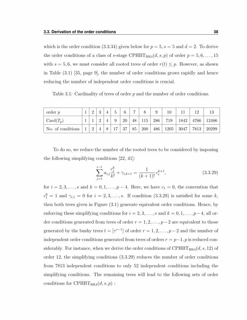
reducing the number of independent order conditions is crucial.
Table 3.1: Cardinality of trees of order p and the number of order conditions.
order p 1 2 3 4 5 6 7 8 9 10 11 12 13
Card(Tp) 1 1 2 4 9 20 48 115 286 719 1842 4766 12486
No. of conditions 1 2 4 8 17 37 85 200 486 1205 3047 7813 20299
To do so, we reduce the number of the rooted trees to be considered by imposing
the following simplifying conditions [22, 41]:
i−1∑j=1
ai,jckjk!
+ γi,k+1 =1
(k + 1)!ck+1i , (3.3.29)
for i = 2, 3, . . . , s and k = 0, 1, . . . , p − 4. Here, we have c1 = 0, the convention that
c01 = 1 and γi,1 = 0 for i = 2, 3, . . . , s. If condition (3.3.29) is satisfied for some k,
then both trees given in Figure (3.1) generate equivalent order conditions. Hence, by
enforcing these simplifying conditions for i = 2, 3, . . . , s and k = 0, 1, . . . , p−4, all or-
der conditions generated from trees of order r = 1, 2, . . . , p−2 are equivalent to those
generated by the bushy trees t = [τ r−1] of order r = 1, 2, . . . , p− 2 and the number of
independent order conditions generated from trees of orders r = p−1, p is reduced con-
siderably. For instance, when we derive the order conditions of CPHBTRK4(d, s, 12) of
order 12, the simplifying conditions (3.3.29) reduces the number of order conditions
from 7813 independent conditions to only 52 independent conditions including the
simplifying conditions. The remaining trees will lead to the following sets of order
conditions for CPHBTRK4(d, s, p) :
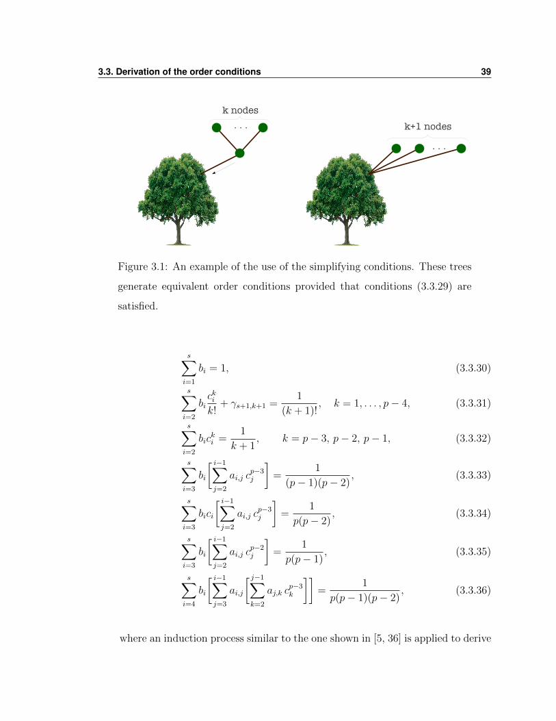
3.3. Derivation of the order conditions 39
. . .k nodes
. . .
k+1 nodes
Figure 3.1: An example of the use of the simplifying conditions. These trees
generate equivalent order conditions provided that conditions (3.3.29) are
satisfied.
s∑i=1
bi = 1, (3.3.30)
s∑i=2
bickik!
+ γs+1,k+1 =1
(k + 1)!, k = 1, . . . , p− 4, (3.3.31)
s∑i=2
bicki =
1
k + 1, k = p− 3, p− 2, p− 1, (3.3.32)
s∑i=3
bi
[ i−1∑j=2
ai,j cp−3j
]=
1
(p− 1)(p− 2), (3.3.33)
s∑i=3
bici
[ i−1∑j=2
ai,j cp−3j
]=
1
p(p− 2), (3.3.34)
s∑i=3
bi
[ i−1∑j=2
ai,j cp−2j
]=
1
p(p− 1), (3.3.35)
s∑i=4
bi
[ i−1∑j=3
ai,j
[ j−1∑k=2
aj,k cp−3k
]]=
1
p(p− 1)(p− 2), (3.3.36)
where an induction process similar to the one shown in [5, 36] is applied to derive
3.3. Derivation of the order conditions 40
the order conditions of CPHBTRK4(d, s, p) of order p. As an example, let us derive
the order conditions for p = 4, 5, 6. For p = 4, the predictors are of order at least 1
and hence the simplifying conditions (3.3.29) are enforced for i = 2, 3, . . . , s and k = 0
only. Hence, we have to consider all trees in Table 3.2 of order r ≤ 4 to derive the
order conditions of CPHBTRK4(d, s, 4) from equations (3.3.16)-(3.3.21). It is worth
mentioning that these order conditions are similar to the order conditions of RK(s, 4)
with added Taylor coefficients. In Table 3.2, φRK(ti) is the elementary weights of
Runge-Kutta method given in Definition 2.1.4 corresponding to a tree ti. Also, r(ti)
and α(ti) are given in Definition 2.1.2 and formula (2.1.6), respectively.
For p = 5, the predictors are of order at least 2 and hence, applying the simplify-
ing conditions for i = 2, 3, . . . , s and k = 0, 1, the following pairs of trees will generate
the same order conditions: (t3, t4), (t5, t6), (t7, t8), (t9, t10), (t11, t12), (t13, t14), (t15, t17),
(t16, t17), (t18, t19), (t20, t21), (t22, t23), (t24, t26), (t25, t26), (t27, t28), (t29, t30), (t31, t34),
(t32, t34), (t33, t34), (t35, t37) and (t26, t27). Then, we can ignore the trees on the left
component of each pair and reduce Table (3.2) to get Table (3.3). Considering all
trees of order r ≤ 5, we can derive the order conditions of CPHBTRK4(d, s, 5).
Finally, for p = 6, the predictors are of order at least 3. Then, applying the
simplifying conditions (3.3.29) for i = 2, 3, . . . , s and k = 0, 1, 2, the following pairs of
trees generate the same order conditions: (t6, t8), (t10, t12), (t14, t17), (t19, t21), (t23, t26),
(t28, t30) and (t34, t37). So, Table (3.3) is reduced to Table (3.4) from which we can
derive the order conditions of CPHBTRK4(d, s, 6).
3.3. Derivation of the order conditions 41
Table 3.2: Notations and some functions on trees of order 1 to 6.
i notation r(ti) φRK(ti) α(ti)
1 τ 1∑i bi 1
2 [τ ] 2∑i bici 1
3 [2τ ]2 3∑ij biaijcj 1
4 [τ2] 3∑i bic
2i 1
5 [3τ ]3 4∑ijk biaijajkck 1
6 [2τ2]2 4∑ij biaijc
2j 1
7 [[τ ]τ ] 4∑ij biciaijcj 3
8 [τ3] 4∑i bic
3i 1
9 [4τ ]4 5∑ijkl biaijajkaklcl 1
10 [3τ2]3 5∑ijk biaijajkc
2k 1
11 [2[τ ]τ ]2 5∑ijk biaijcjajkck 3
12 [2τ3]2 5∑ij biaijc
3j 1
13 [[2τ ]2τ ] 5∑ijk biciaijajkck 4
14 [[τ2]τ ] 5∑ij biciaijc
2j 4
15 [[τ ]2] 5∑i bi(
∑j aijcj)
2 3
16 [[τ ]τ2] 5∑ij bic
2i aijcj 6
17 [τ4] 5∑i bic
4i 1
18 [5τ ]5 6∑ijklm biaijajkaklalmcm 1
19 [4τ2]4 6∑ijkl biaijajkaklc
2l 1
20 [3[τ ]τ ]3 6∑ijkl biaijajkckaklcl 3
21 [3τ3]3 6∑ijk biaijajkc
3k 1
22 [2[2τ ]2τ ]2 6∑ijkl biaijcjajkaklcl 4
23 [2[τ2]τ ]2 6∑ijk biaijcjajkc
2k 4
24 [2[τ ]2]2 6∑i biaij(
∑k ajkck)2 3
25 [2[τ ]τ2]2 6∑ijk biaijc
2jajkck 6
26 [2τ4]2 6∑ij biaijc
4j 1
27 [[3τ ]3τ ] 6∑ijkl biciaijajkaklcl 5
28 [[2τ2]2τ ] 6∑ijk biciaijajkc
2k 5
29 [[[τ ]τ ]τ ] 6∑ijk biciaijcjajkck 15
30 [[τ3]τ ] 6∑ij biciaijc
3j 5
31 [[2τ ]2[τ ]] 6∑i bi(
∑jk aijajkck)(
∑j aijcj) 10
32 [[τ2][τ ]] 6∑i bi(
∑j aijc
2j )(
∑j aijcj) 10
33 [[2τ ]2τ2] 6∑ijk bic
2i aijajkck 10
34 [[τ2]τ2] 6∑ij bic
2i aijc
2j 10
35 [[τ ]2τ ] 6∑i bici(
∑j aijcj)
2 15
36 [[τ ]τ3] 6∑ijk bic
3i aijcj 10
37 [τ5] 6∑i bic
5i 1

3.3. Derivation of the order conditions 42
Table 3.3: Notations and some functions on the remaining trees after apply-
ing the simplifying conditions (3.3.29) for k = 0, 1.
i notation r(ti) φRK(ti) α(ti)
1 τ 1∑i bi 1
2 [τ ] 2∑i bici 1
4 [τ2] 3∑i bic
2i 1
6 [2τ2]2 4∑ij biaijc
2j 1
8 [τ3] 4∑i bic
3i 1
10 [3τ2]3 5∑ijk biaijajkc
2k 1
12 [2τ3]2 5∑ij biaijc
3j 1
14 [[τ2]τ ] 5∑ij biciaijc
2j 4
17 [τ4] 5∑i bic
4i 1
19 [4τ2]4 6∑ijkl biaijajkaklc
2l 1
21 [3τ3]3 6∑ijk biaijajkc
3k 1
23 [2[τ2]τ ]2 6∑ijk biaijcjajkc
2k 4
26 [2τ4]2 6∑ij biaijc
4j 1
28 [[2τ2]2τ ] 6∑ijk biciaijajkc
2k 5
30 [[τ3]τ ] 6∑ij biciaijc
3j 5
34 [[τ2]τ2] 6∑ij bic
2i aijc
2j 10
37 [τ5] 6∑i bic
5i 1

3.4. Formulation of CPHBTRK4(d, s, p) methods in Shu-Osher form 43
Table 3.4: Notations and some functions on the remaining trees after apply-
ing the simplifying conditions (3.3.29) for k = 0, 1, 2.
i notation r(ti) φRK(ti) α(ti)
1 τ 1∑i bi 1
2 [τ ] 2∑i bici 1
4 [τ2] 3∑i bic
2i 1
8 [τ3] 4∑i bic
3i 1
12 [2τ3]2 5∑ij biaijc
3j 1
17 [τ4] 5∑i bic
4i 1
21 [3τ3]3 6∑ijk biaijajkc
3k 1
26 [2, τ4]2 6∑ij biaijc
4j 1
30 [[τ3]τ ] 6∑ij biciaijc
3j 5
37 [τ5] 6∑i bic
5i 1
3.4 Formulation of CPHBTRK4(d, s, p) methods in
Shu-Osher form
Let σ = [0, c2, c3, . . . , cs]T define the s − 1 off-step points xn + cj∆x, j = 2, 3, . . . , s.
Then, F1 = fn and Fj := f(xn + cj∆x, Yj), j = 2, 3, . . . , s, where we always choose
c1 = 0.
To be able to write CPHBTRK4(d, s, p) methods as a convex combination of the
forward Euler expanded series FES(d) method (3.1.2), we restrict ourself to nonneg-
ative coefficient triplets (A, b,γ0) and rewrite the formulas (3.2.1) and (3.2.2) in the
modified Shu-Osher form as in [53, 18] for 2 ≤ i ≤ s+ 1,
Yi = viyn +
[ i−1∑j=1
αi,jYj + ∆x βi,jFj
]+
d∑m=2
(∆x)mδi,m y(m)n ,
yn+1 = Ys+1, (3.4.1)
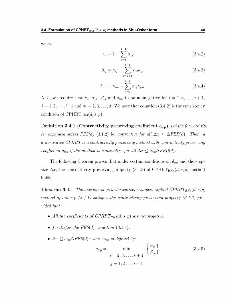
3.4. Formulation of CPHBTRK4(d, s, p) methods in Shu-Osher form 44
where
vi = 1−i−1∑j=1
αij, (3.4.2)
βij = aij −i−1∑l=j+1
αilalj, (3.4.3)
δim = γim −i−1∑j=1
αijγjm. (3.4.4)
Also, we require that vi, αij, βij and δim to be nonnegative for i = 2, 3, . . . , s + 1,
j = 1, 2, . . . , i−1 and m = 2, 3, . . . , d. We note that equation (3.4.2) is the consistency
condition of CPHBTRK4(d, s, p).
Definition 3.4.1 (Contractivity preserving coefficient cfcp) Let the forward Eu-
ler expanded series FES(d) (3.1.2) be contractive for all ∆x ≤ ∆FED(d). Then, a
d-derivative CPHBT is a contractivity preserving method with contractivity preserving
coefficient cfcp if the method is contractive for all ∆x ≤ cfcp∆FED(d).
The following theorem proves that under certain conditions on δim and the step-
size ∆x, the contractivity preserving property (3.1.3) of CPHBTRK4(d, s, p) method
holds.
Theorem 3.4.1 The new one-step, d-derivative, s-stages, explicit CPHBTRK4(d, s, p)
method of order p (3.4.1) satisfies the contractivity preserving property (3.1.3) pro-
vided that
• All the coefficients of CPHBTRK4(d, s, p) are nonnegative.
• f satisfies the FES(d) condition (3.1.4).
• ∆x ≤ cfcp∆FES(d) where cfcp is defined by:
cfcp = min
i = 2, 3, . . . , s+ 1
j = 1, 2 . . . , i− 1
αijβij
. (3.4.5)
3.4. Formulation of CPHBTRK4(d, s, p) methods in Shu-Osher form 45
• δi,m satisfies the following conditions:
δi,mαi,1≤[
1
cfcp
]m1
m!, (3.4.6)
for i = 2, 3, . . . , s+ 1 and m = 2, 3, . . . , d.
Proof: We rewrite the stages of the new CPHBTRK4(d, s, p) in (3.4.1) as follows:
Yi = viyn +i−1∑j=2
αi,j
[Yj + ∆x
βi,jαi,j
Fj
]+ αi,1
[yn + ∆x
βi,1αi,1
fn
+d∑
m=2
(∆x)mδi,mαi,1
y(m)n
], i = 2, 3, . . . , s+ 1
Then, by applying the same norm or convex functional ‖ · ‖ as in (3.1.4) we get
‖Yi − Yi‖ =
∥∥∥∥vi(yn − yn) +i−1∑j=2
αi,j
[Yj + ∆x
βi,jαi,j
Fj − (Yj + ∆xβi,jαi,j
Fj)
]
+ αi,1
[yn + ∆x
βi,1αi,1
fn +d∑
m=2
(∆x)mδi,mαi,1
y(m)n − (yn + ∆x
βi,1αi,1
fn +d∑
m=2
(∆x)mδi,mαi,1
y(m)n )
]∥∥∥∥≤ vi
∥∥∥∥yn − yn∥∥∥∥+i−1∑j=2
αi,j
∥∥∥∥Yj + ∆xβi,jαi,j
Fj − (Yj + ∆xβi,jαi,j
Fj)
∥∥∥∥+ αi,1
∥∥∥∥yn + ∆xβi,1αi,1
fn +d∑
m=2
(∆x)mδi,mαi,1
y(m)n − (yn + ∆x
βi,1αi,1
fn +d∑
m=2
(∆x)mδi,mαi,1
y(m)n )
∥∥∥∥.However, by the assumptions of the theorem, ∆x
βi,jαi,j≤ ∆FES(d) and
(∆x)mδi,mαi,1≤[
∆xcfcp
]m1m!
. Then, inequality (3.1.4) holds and we get
‖Yi − Yi‖ ≤ vi ‖yn − yn‖+i−1∑j=2
αi,j ‖yn − yn‖+ αi,1 ‖yn − yn‖
= ‖yn − yn‖ .
This is valid for i = 2, 3, . . . , s + 1. Hence, the contractivity preserving property
(3.1.3) follows by taking i = s+ 1.
3.5. CPHBTRK4(d, s, p) in vector notation 46
Remark 3.4.1 In the above theorem:
• We use the notations fn = f(yn) and Fj = f(Yj).
• We use the convention thatαij0
= +∞ in the evaluation of cfcp in (3.4.5).
• Enforcing the conditions of the theorem with the order conditions, which are
derived in Section 3.3, will generate a feasible CPHBTRK4(d, s, p) method with
a feasible contractivity preserving coefficient cfcp defined in (3.4.5).
• We are interested in an optimal CPHBTRK4(d, s, p) with an optimal contractiv-
ity preserving coefficient ccp, i.e., with the largest contractivity preserving coef-
ficient that will allow a maximum stepsize while maintaining the contractivity
preserving property (3.1.3).
• To improve the optimization process of the coefficient of CPHBTRK4(d, s, p), we
need to present the method in different forms.
3.5 CPHBTRK4(d, s, p) in vector notation
We are interested in a more compact form of the modified Shu-Osher form of CPHBTRK4
(d, s, p) (3.4.1). Let v ∈ Rs+1, v = [0, v2, v3, . . . , vs+1]T , and define the matrices
α,β ∈ R(s+1)×(s+1), and δ ∈ R(s+1)×(d−1) as follows:
(α)ij =
αij i = 2, 3, . . . , s+ 1, j = 1, 2, . . . , i− 1
0 otherwise,
(3.5.1)
(β)ij =
βij i = 2, 3, . . . , s+ 1, j = 1, 2, . . . , i− 1
0 otherwise,
(3.5.2)
(δ)ij =
δim i = 2, 3, . . . , s+ 1, m = 2, 3, . . . , d,
0 otherwise,
(3.5.3)
3.6. The Butcher form in vector notation 47
Also, let Y ,F ∈ R(s+1)×N and fB ∈ R(d−1)×N :
Y = [Y1, Y2, . . . , Ys+1]T , F = [F1, F2, . . . , Fs+1]T ,
fB = [(∆x)2y(2)n , (∆x)3y(3)
n , . . . , (∆x)dy(d)n ]T ,
with the following N -vectors: Yj, Fj for j = 1, 2, . . . , s + 1, y(j)n for j = 2, 3, . . . , d,
Y1 = yn, F1 = fn, Ys+1 = yn+1 and Fs+1 = fn+1, where N is the dimension of ODE
system. Hence, we can rewrite CPHBTRK4(d, s, p) (3.4.1) compactly as follows:
Y = vyTn +αY + ∆xβF + δfB,
yn+1 = Ys+1.(3.5.4)
Note that the consistency condition (3.4.2) becomes
v +αes+1 = es+1, (3.5.5)
where the (s+ 1)-vector es+1 is
es+1 = [1, 1, 1, . . . , 1]T ∈ Rs+1.
3.6 The Butcher form in vector notation
This subsection describes a generalized result for the new CPHBTRK4(d, s, p), using
the result for RK methods, following closely section 3.2.1 of [18, pp. 31–32] and our
published work [42].
Recall that the coefficients matrix α ∈ R(s+1)×(s+1) is defined in (3.5.1). If we let
α = 0, then the Shu-Osher form (3.5.4) becomes,
Y = vyTn + ∆xβF + δfB,
yn+1 = Ys+1.(3.6.1)
which is the Butcher form (3.2.1) and (3.2.2). The elements v, β, δ of (3.6.1) are then
denoted by v0, β0, γ0, respectively. Here, the consistency condition (3.5.5) becomes
v0 = es+1. (3.6.2)
3.6. The Butcher form in vector notation 48
Hence the Butcher form (3.6.1) can be rewritten as
Y = es+1yTn + ∆xβ0F + γ0fB,
yn+1 = Ys+1.(3.6.3)
To find the relation between the Shu-Osher coefficients and the Butcher coefficients,
we can solve (3.5.4) for Y ,
Y = (I −α)−1 vyTn + ∆x (I −α)−1 βF + (I −α)−1 δfB, (3.6.4)
where (I − α) is invertible since α is a strictly lower triangular matrix. Comparing
(3.6.4) with (3.6.3), we have the following relations between the modified Shu-Osher
coefficients and the Butcher coefficients,
v0 = es+1 = (I −α)−1 v,
β0 = (I −α)−1 β,
γ0 = (I −α)−1 δ.
(3.6.5)
Remark 3.6.1 • These relations will enable us to transform a Shu-Osher form
of CPHBTRK4(d, s, p) into its Butcher form and vice versa.
• The relations (3.6.5) confirm the previously derived equations (3.4.2)-(3.4.4).
• The form (3.6.3) is the Butcher form (3.2.1) and (3.2.2) with γ0 defined in
(3.2.5) and the following matrix,
β0 =
0 0 0 0 0 0
a2,1 0 0 0 0 0
a3,1 a3,2 0 0 0 0...
.... . . 0 0 0
as,1 as,2 . . . as,s−1 0 0
b1 b2 . . . bs−1 bs 0
. (3.6.6)
3.7. CPHBTRK4(d, s, p) in the canonical Shu-Osher form 49
3.7 CPHBTRK4(d, s, p) in the canonical Shu-Osher
form
A more useful way to represent the results of CPHBTRK4(d, s, p) is to consider the
canonical form of (3.5.4). To derive its canonical Shu-Osher form, we require the ratio
r =αi,jβi,j
to be constant for i = 2, 3, 4, . . . , s + 1 and j = 1, 2, 3, . . . , i − 1, such that
βi,j 6= 0 [18, 42]. Generally, if the particular Shu-Osher form of α and β is sparse, the
Shu-Osher form of CPHBTRK4(d, s, p) will allow a reduced-storage implementation,
similar to the work of Ketcheson on optimal explicit SSP Runge-Kutta methods [30].
We shall denote the coefficient matrices of this special form by αr, βr, and require
that αr = rβr. Substituting this relation into (3.6.5), we can solve for βr in terms of
β0 and r. Thus we find
(I − rβr)−1 βr = β0 ⇔ βr = β0 − rβrβ0
⇔ βr (I + rβ0) = β0.
Hence, the coefficients for this form are given by
vr = (I + rβ0)−1 v0 = (I −αr)v0, (3.7.1)
βr = β0 (I + rβ0)−1 = β0 (I −αr) , (3.7.2)
αr = rβr = rβ0 (I + rβ0)−1 = rβ0 (I −αr) , (3.7.3)
δr = (I + rβ0)−1 γ0 = (I −αr)γ0, (3.7.4)
where the identity (I −αr) = (I + rβ0)−1 follows from
(I −αr) (I + rβ0) = (I − rβr) (I + rβ0)
= I + rβ0 − rβr − r2βrβ0 = I
since rβr = rβ0 − r2βrβ0.
3.7. CPHBTRK4(d, s, p) in the canonical Shu-Osher form 50
Then, using (3.6.5) and (3.7.2), we have
βr = β0 (I + rβ0)−1
= β0 (I −αr)
= (I −αr)β0
= (I + rβ0)−1 β0. (3.7.5)
As in [18], we will refer to the form obtained by the relations (3.7.1)–(3.7.4) as
the canonical Shu-Osher form of CPHBTRK4(d, s, p) :
Y = vryTn +αrY + ∆xβrF + δrfB. (3.7.6)
Then, (3.7.6) can be written in terms of the Butcher array:
Y =[(I + rβ0)−1 v0y
Tn
]+[rβ0 (I + rβ0)−1 Y
+ ∆xβ0 (I + rβ0)−1 F]
+[(I + rβ0)−1 γ0fB
]. (3.7.7)
Using (3.7.5) and (3.7.7), we have
Y = (I + rβ0)−1 [v0yTn + β0 (rY + ∆xF ) + γ0fB
]. (3.7.8)
Here the consistency condition is
(I + rβ0)−1 v0 + r (I + rβ0)−1 β0es+1 = es+1. (3.7.9)
Remark 3.7.1 • Since β0 is strictly lower triangular, then I + rβ0 is invertible
and the transformations (3.7.1)-(3.7.4) are always defined.
• For r = 0, the consistency condition (3.7.9) is equivalent to (3.6.2) and the
canonical Shu-Osher form (3.7.6) or (3.7.8) corresponds to the Butcher form
(3.6.3), with coefficient vector v0 and coefficient matrices β0 and γ0.
3.7. CPHBTRK4(d, s, p) in the canonical Shu-Osher form 51
• Generally, the sparse canonical Shu-Osher forms (3.7.6) or (3.7.8) will allow for
reduced-storage implementation which enhance the performance of CPHBTRK4
(d, s, p).
• The relations (3.7.1)–(3.7.4) will enable us to transform easily a Butcher form
of CPHBTRK4(d, s, p) method into its canonical Shu-Osher form and vice versa.
Recall that in Theorem 3.4.1, the contractivity preserving coefficient cfcp is given in
(3.4.5) as a minimum function min(·). Indeed, we are interested in optimal CPHBT
methods with maximal cfcp to maximize the step-size in (3.4.5). However, the min(·)
function is not smooth or even sensitive to its parameters which will generate various
problems especially if the optimization process uses gradient information. To avoid
these issues, we state an improved version of Theorem 3.4.1 where we use a modified
form of the canonical Shu-Osher form in which we consider a fixed ratio
r =αijβij
i = 3, 4, . . . , s+ 1, j = 2, 3, . . . , i− 1,
such that the feasible contractivity preserving coefficient cfcp defined in 3.4.1 is equal
to r and should satisfy
cfcp = r ≤ ri1 =αi1βi1
i = 2, 3, . . . , s+ 1.
Moreover, conditions (3.4.6) with cfcp replaced by ri1 = αi1βi1
are imposed on δim for
i = 2, 3, . . . , s+ 1 and m = 2, 3, . . . , d. We then get the following theorem:
Theorem 3.7.1 The new one-step, d-derivative, s-stages, explicit CPHBTRK4(d, s, p)
method (3.4.1) satisfies the contractivity preserving property (3.1.3) provided that
• All the coefficients of CPHBTRK4(d, s, p) are nonnegative.
• f satisfies the FES(d) condition (3.1.4).
3.8. Formulation of the optimization problem of CPHBTRK4(d, s, p) 52
• ∆x ≤ cfcp∆FES(d) where ∆FES(d) is given in (3.1.4) and cfcp is defined by:
cfcp = r =
αijβij
i = 3, 4, . . . , s+ 1, j = 2, 3, . . . , i− 1. (3.7.10)
• r satisfies the conditions:
r ≤ ri1 =αi1βi1
i = 2, 3, . . . , s+ 1. (3.7.11)
• δi,m satisfies the following conditions:
δi,mrmi1m!− αi,1 ≤ 0 i = 2, 3, . . . , s+ 1, m = 2, 3, . . . , d. (3.7.12)
The conditions on δi,m in the form (3.7.12) are more numerically stable and will
enhance the performance of the optimization software. The proof of Theorem 3.7.1
is a straightforward extension of the proof of Theorem 3.4.1.
3.8 Formulation of the optimization problem of
CPHBTRK4(d, s, p)
As we mentioned before, any set of nonnegative coefficients (vr,αr,βr, δr) satisfy-
ing the order conditions (3.3.30)-(3.3.36), the simplifying conditions (3.3.29) and the
conditions of Theorem 3.7.1 will generate a feasible CPHBTRK4(d, s, p) of order p.
In this section, we formulate an optimization process to find an optimal CPHBTRK4
(d, s, p) with optimal contractivity preserving coefficient ccp as follows:
maximizevr,αr,βr,δr
r = ccp (3.8.1)
subject to
(I + rβ0)−1 v0 ≥ 0, (3.8.2)
(I + rβ0)−1 β0 ≥ 0, (3.8.3)
3.8. Formulation of the optimization problem of CPHBTRK4(d, s, p) 53
(I + rβ0)−1 γ0 ≥ 0, (3.8.4)
ci ≤ 1 i = 2, 3, . . . , s+ 1, (3.8.5)
r ≤ ri1 i = 2, 3, . . . , s+ 1, (3.8.6)
δi,mrmi1m!− αi,1 ≤ 0,
i = 2, 3, . . . , s+ 1,
m = 2, 3, . . . , d,
(3.8.7)
together with
• The simplifying conditions (3.3.29),
• The set of order conditions (3.3.30)-(3.3.36),
where inequalities (3.8.2)-(3.8.4) are taken component-wise and the coefficient ma-
trices v0,β0,γ0 and δ are defined in equations (3.6.5), (3.4.4) and (3.5.3). However,
the objective function in this form is not smooth and hence using an optimization
method depending on the gradient will not give reliable results. Moreover, Spiteri
[56] showed that even optimization methods that do not use gradient information
fail to converge to the same optimum. To avoid this problem, we follow a standard
reformulation of the optimization process by introducing a dummy parameter z and
the objective function
F : R× Rs+1 × R(s+1)×(s+1) × R(s+1)×(s+1) × R(s+1)×(d−1) → R
such that F (z,v,α,β, δ) = z. (3.8.8)
Then the optimization problem is as follows
maximizez,v,α,β,δ
F (z,v,α,β, δ) = z (3.8.9)
subject to
• The constraint αij − zβij = 0 for i = 3, 4, . . . , s+ 1, j = 2, 3, . . . , i− 1,
3.9. Construction of optimal CPHBTRK4(d, s, p) 54
• The constraints (3.8.2)-(3.8.7) with r replaced by z,
• The simplifying conditions (3.3.29),
• The set of order conditions (3.3.30)-(3.3.36).
3.9 Construction of optimal CPHBTRK4(d, s, p)
The objective function (3.8.8) of the optimization process (3.8.9) is a projection func-
tion and hence it is continuous. Let FS ⊂ R × Rs+1 × R(s+1)×(s+1) × R(s+1)×(s+1) ×
R(s+1)×(d−1) be the feasible set of the optimization problem (3.8.9). We managed to
find bounds for all the variables in the feasible set FS, component-wise, except the
first component corresponding to z, in particular, FS ⊂ R×[0, 1]s+1×[0, 1](s+1)×(s+1)×
[0, 1](s+1)×(s+1) × [0, 1](s+1)×(d−1). However, following [55, 54, 18] and our published
work in [42], our numerical search for optimal solutions is computationally stable
and the variable z is bounded. Since CPHBTRK4(d, s, p) methods contain many free
parameters, the MATLAB Optimization Toolbox was used to search for the methods
with largest contractivity preserving coefficient ccp. Several authors, [55, 54, 18], have
successfully used this technique to find optimal Runge-Kutta methods. In particu-
lar, the MATLAB function fmincon from the Optimization Toolbox is used to solve
the optimization problem above. Although no analytic proof of global optimality is
provided, the obtained methods are a result of performing an extensive numerical
search with a large number of initial points similar to Spiteri and Ruuth’s approach
in [55, 54]. In this work, depending on the size of the feasible set, the MATLAB Op-
timization Toolbox was used to tolerance in the range (10−15, 10−12) on the objective
function provided that all the constraints were satisfied to tolerance in a the range
(10−17, 10−14).
We managed to obtain s-stage, d-derivative CPHBTRK4(d, s, p) methods of order
p for p = 5, 6, . . . , 15, s = 5, 6 and d = 2, 3, . . . , 13. In Tables 3.5, we summarize these
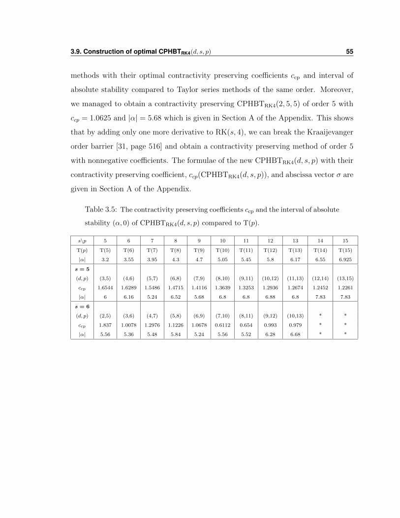
3.9. Construction of optimal CPHBTRK4(d, s, p) 55
methods with their optimal contractivity preserving coefficients ccp and interval of
absolute stability compared to Taylor series methods of the same order. Moreover,
we managed to obtain a contractivity preserving CPHBTRK4(2, 5, 5) of order 5 with
ccp = 1.0625 and |α| = 5.68 which is given in Section A of the Appendix. This shows
that by adding only one more derivative to RK(s, 4), we can break the Kraaijevanger
order barrier [31, page 516] and obtain a contractivity preserving method of order 5
with nonnegative coefficients. The formulae of the new CPHBTRK4(d, s, p) with their
contractivity preserving coefficient, ccp(CPHBTRK4(d, s, p)), and abscissa vector σ are
given in Section A of the Appendix.
Table 3.5: The contractivity preserving coefficients ccp and the interval of absolute
stability (α, 0) of CPHBTRK4(d, s, p) compared to T(p).
s\p 5 6 7 8 9 10 11 12 13 14 15
T(p) T(5) T(6) T(7) T(8) T(9) T(10) T(11) T(12) T(13) T(14) T(15)
|α| 3.2 3.55 3.95 4.3 4.7 5.05 5.45 5.8 6.17 6.55 6.925
s = 5
(d, p) (3,5) (4,6) (5,7) (6,8) (7,9) (8,10) (9,11) (10,12) (11,13) (12,14) (13,15)
ccp 1.6544 1.6289 1.5486 1.4715 1.4116 1.3639 1.3253 1.2936 1.2674 1.2452 1.2261
|α| 6 6.16 5.24 6.52 5.68 6.8 6.8 6.88 6.8 7.83 7.83
s = 6
(d, p) (2,5) (3,6) (4,7) (5,8) (6,9) (7,10) (8,11) (9,12) (10,13) * *
ccp 1.837 1.0078 1.2976 1.1226 1.0678 0.6112 0.654 0.993 0.979 * *
|α| 5.56 5.36 5.48 5.84 5.24 5.56 5.52 6.28 6.68 * *
Chapter 4
Numerical results for the designed
CPHBTRK4(d, s, p) methods
obtained from T(d) and RK(s,4)
methods
4.1 Introduction
In this chapter, we will test the methods derived in chapter 3 and compare them
to different well known and widely used numerical methods. The s-stage, one step,
d-derivatives CPHBTRK4(d, s, p) method of order p requires the evaluation of the d
derivatives y(1), y(2), . . . , y(d) at each integration step. These derivatives were com-
puted recursively using the automatic differentiation technique that is described
briefly in Section 2.2.1 and in more details in [22, page 46-49] and [34]. All nu-
merical tests and simulations were obtained using two systems: a Macbook pro 6,2
with a 10.6.8 Mac OSX, a 2.53 GHz Intel Core i5 processor and a 4 GB 1067 MHz
DDR3 memory. The second machine is a Sun Microsystems with AMD Opteron(tm)
56
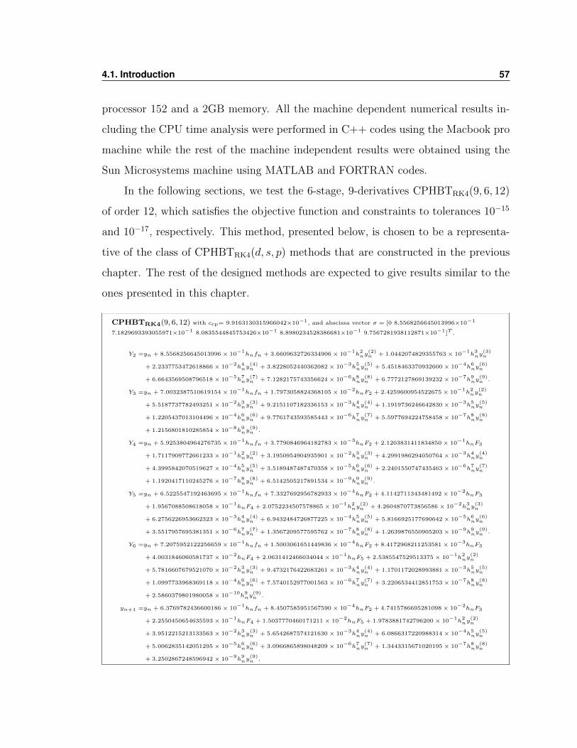
4.1. Introduction 57
processor 152 and a 2GB memory. All the machine dependent numerical results in-
cluding the CPU time analysis were performed in C++ codes using the Macbook pro
machine while the rest of the machine independent results were obtained using the
Sun Microsystems machine using MATLAB and FORTRAN codes.
In the following sections, we test the 6-stage, 9-derivatives CPHBTRK4(9, 6, 12)
of order 12, which satisfies the objective function and constraints to tolerances 10−15
and 10−17, respectively. This method, presented below, is chosen to be a representa-
tive of the class of CPHBTRK4(d, s, p) methods that are constructed in the previous
chapter. The rest of the designed methods are expected to give results similar to the
ones presented in this chapter.
CPHBTRK4(9, 6, 12) with ccp= 9.9163130315966042×10⁻¹, and abscissa vector σ = [0 8.5568256645013996×10⁻¹
7.1829693393055971×10⁻¹ 8.0835544845753426×10⁻¹ 8.8980234528386681×10⁻¹ 9.7567281938112871×10⁻¹]T .
Y2 =yn + 8.5568256645013996 × 10⁻¹hnfn + 3.6609632726334906 × 10
−1h2ny
(2)n + 1.0442074829355763 × 10
−1h3ny
(3)n
+ 2.2337753472618866 × 10⁻²h4ny
(4)n + 3.8228052440362082 × 10
−3h5ny
(5)n + 5.4518463370932600 × 10
−4h6ny
(6)n
+ 6.6643569508796518 × 10⁻⁵h7ny
(7)n + 7.1282175743356624 × 10
−6h8ny
(8)n + 6.7772127869139232 × 10
−7h9ny
(9)n .
Y3 =yn + 7.0032387510619154 × 10⁻¹hnfn + 1.7973058824368105 × 10
−2hnF2 + 2.4259600954522675 × 10
−1h2ny
(2)n
+ 5.5187737782493251 × 10⁻²h3ny
(3)n + 9.2151107182336153 × 10
−3h4ny
(4)n + 1.1919736246642830 × 10
−3h5ny
(5)n
+ 1.2205437013104496 × 10⁻⁴h6ny
(6)n + 9.7761743593585443 × 10
−6h7ny
(7)n + 5.5977694224758458 × 10
−7h8ny
(8)n
+ 1.2156801810285854 × 10⁻⁸h9ny
(9)n .
Y4 =yn + 5.9253804964276735 × 10⁻¹hnfn + 3.7790846964182783 × 10
−3hnF2 + 2.1203831411834850 × 10
−1hnF3
+ 1.7117909772661233 × 10⁻¹h2ny
(2)n + 3.1950954904935901 × 10
−2h3ny
(3)n + 4.2991986294050764 × 10
−3h4ny
(4)n
+ 4.3995842070519627 × 10⁻⁴h5ny
(5)n + 3.5189487487470358 × 10
−5h6ny
(6)n + 2.2401550747435463 × 10
−6h7ny
(7)n
+ 1.1920417110245276 × 10⁻⁷h8ny
(8)n + 6.5142505217891534 × 10
−9h9ny
(9)n .
Y5 =yn + 6.5225547192463695 × 10⁻¹hnfn + 7.3327692956782933 × 10
−4hnF2 + 4.1142711343481492 × 10
−2hnF3
+ 1.9567088508618058 × 10⁻¹hnF4 + 2.0752234507578865 × 10
−1h2ny
(2)n + 4.2604870773856586 × 10
−2h3ny
(3)n
+ 6.2756226953662323 × 10⁻³h4ny
(4)n + 6.9432484726877225 × 10
−4h5ny
(5)n + 5.8166925177690642 × 10
−5h6ny
(6)n
+ 3.5517957695381351 × 10⁻⁶h7ny
(7)n + 1.3567209577595762 × 10
−7h8ny
(8)n + 1.2639876550905203 × 10
−9h9ny
(9)n .
Y6 =yn + 7.2075952122256659 × 10⁻¹hnfn + 1.5003061651449836 × 10
−4hnF2 + 8.4172968211253581 × 10
−3hnF3
+ 4.0031846060581737 × 10⁻²hnF4 + 2.0631412466034044 × 10
−1hnF5 + 2.5385547529513375 × 10
−1h2ny
(2)n
+ 5.7816607679521070 × 10⁻²h3ny
(3)n + 9.4732176422683261 × 10
−3h4ny
(4)n + 1.1701172028993881 × 10
−3h5ny
(5)n
+ 1.0997733968369118 × 10⁻⁴h6ny
(6)n + 7.5740152977001563 × 10
−6h7ny
(7)n + 3.2206534412851753 × 10
−7h8ny
(8)n
+ 2.5860379801980058 × 10⁻¹⁰
h9ny
(9)n .
yn+1 =yn + 6.3769782436600186 × 10⁻¹hnfn + 8.4507585951567590 × 10
−4hnF2 + 4.7415786695281098 × 10
−2hnF3
+ 2.2550450654635593 × 10⁻¹hnF4 + 1.5037770460171211 × 10
−2hnF5 + 1.9783881742796200 × 10
−1h2ny
(2)n
+ 3.9512215213133563 × 10⁻²h3ny
(3)n + 5.6542687574121630 × 10
−3h4ny
(4)n + 6.0866317220988314 × 10
−4h5ny
(5)n
+ 5.0062835142051295 × 10⁻⁵h6ny
(6)n + 3.0966865898048209 × 10
−6h7ny
(7)n + 1.3443315671020195 × 10
−7h8ny
(8)n
+ 3.2502867248596942 × 10⁻⁹h9ny
(9)n .
4.2. Stability region of CPHBTRK4(d, s, p) 58
Our method is compared with the widely used Dormand-Prince Runge-Kutta
pair , DP(8,7)13M, of order 8 [43], Taylor method of order 12, T(12), and the Taylor
method of order 12 introduced by Martin Lara, T(12)L [34]. Also, we will use the
standard bank of differential equations test problems, DETEST, which is used in the
literature as a comparison tool of higher order numerical methods [27]. In particular,
we concentrate on the 20 nonstiff DESTEST problems in classes A, B, D, E which
are described briefly in Section 2.3.
4.2 Stability region of CPHBTRK4(d, s, p)
To obtain the region of absolute stability of CPHBTRK4(d, s, p), we write the method
in Butcher form in compact vector notation
Y = es+1yTn + hβ0F + γ0fB, (4.2.1)
yn+1 = Ys+1. (4.2.2)
where
Y = [Y1, Y2, . . . , Ys+1]T , F = [F1, F2, . . . , Fs+1]T ,
fB = [h2y(2)n , h3y(3)
n , . . . , hdy(d)n ]T ,
Definition 4.2.1 [23] Given the Dahlquist test equation
y′ = λy, y0 = 1,
the stability region of a numerical method is defined as
S = z ∈ C : |R(z)| ≤ 1, z = λh.
where R(z) is the stability function of the numerical method yn+1 = R(z)yn.
4.2. Stability region of CPHBTRK4(d, s, p) 59
Applying method (4.2.2) to the Dahlquist test equation we get
Y = es+1yn + zβ0Y + γ0zyn, (4.2.3)
yn+1 = Ys+1. (4.2.4)
where z = [z2, z3, . . ., zd]T . Solving (4.2.3) for Y , we get the following
(I − zβ0)Y = (es+1 + γ0z)yn (4.2.5)
Y = (I − zβ0)−1(es+1 + γ0z)yn, (4.2.6)
where (I−zβ0) is invertible since β0 is a strictly lower triangular matrix by definition.
Hence, the stability function of CPHBTRK4(d, s, p) is
R(z) =[(I − zβ0)−1
]s+1
(es+1 + γ0z), (4.2.7)
where [X]s+1 denotes the (s + 1)-th row of a matrix X. Also, another form of the
stability function can be obtained from the Butcher form (3.2.1)-(3.2.2) as R(z) =
1 +∑d+2
j=1 sjzj where
s1 =∑j
bj,
s2 =∑j
bj∑k
ajk + γs+1,2,
s3 =∑j
bj(∑
k
ajk∑l
akl + γj,2)
+ γs+1,3,
sq =∑j
bj(∑
k
ajkγk,q−2 + γj,q−1
)+ γs+1,q for q = 4, 5, . . . , d+ 2.
We used the scanning technique [33] to plot the region of absolute stability of CPHBTRK4
(9, 6, 12) which is easier to implement than the boundary locus technique. In Figure
(4.1), we have the region of absolute stability of CPHBTRK4(9, 6, 12) with an interval
of absolute stability (−6.28, 0) compared to Taylor method of order 12, T(12), with
interval of absolute stability (−5.72, 0).
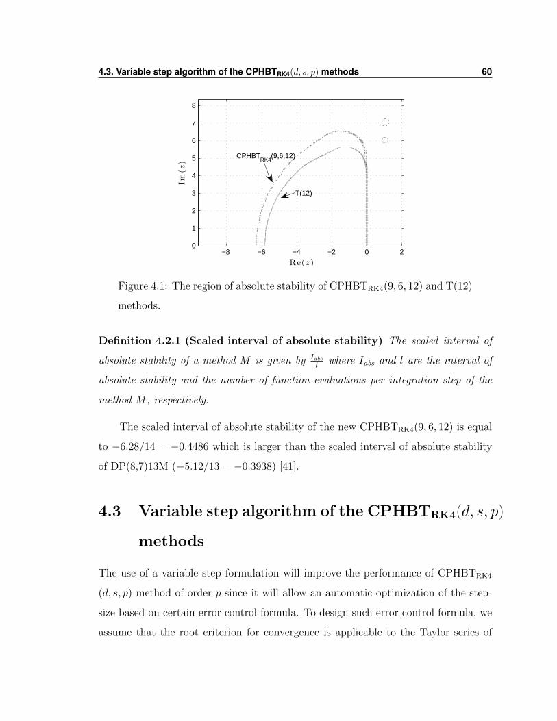
4.3. Variable step algorithm of the CPHBTRK4(d, s, p) methods 60
−8 −6 −4 −2 0 20
1
2
3
4
5
6
7
8
Re(z )
Im(z
)
T(12)
CPHBTRK4
(9,6,12)
Figure 4.1: The region of absolute stability of CPHBTRK4(9, 6, 12) and T(12)
methods.
Definition 4.2.1 (Scaled interval of absolute stability) The scaled interval of
absolute stability of a method M is given by Iabsl
where Iabs and l are the interval of
absolute stability and the number of function evaluations per integration step of the
method M , respectively.
The scaled interval of absolute stability of the new CPHBTRK4(9, 6, 12) is equal
to −6.28/14 = −0.4486 which is larger than the scaled interval of absolute stability
of DP(8,7)13M (−5.12/13 = −0.3938) [41].
4.3 Variable step algorithm of the CPHBTRK4(d, s, p)
methods
The use of a variable step formulation will improve the performance of CPHBTRK4
(d, s, p) method of order p since it will allow an automatic optimization of the step-
size based on certain error control formula. To design such error control formula, we
assume that the root criterion for convergence is applicable to the Taylor series of
4.3. Variable step algorithm of the CPHBTRK4(d, s, p) methods 61
order p as follows:p√‖Y [p]‖∞hp < k < 1 ∀p ≥ p0 (4.3.1)
for some number p0 where h is the step-size and y(x+ h) ≈∑p
i=0 Y[i]hi =
∑pi=0
y(i)
i!hi
is the Taylor series method of order p, T(p). If Ep denotes the local truncation error
at order p, then
|Ep| < kp+1 + kp+2 + . . . = kp+1(1 + k + k2 + . . .) =kp+1
1− k. (4.3.2)
Our goal is to design a step control algorithm that takes a user defined tolerance,
TOL, and optimize the step-size to obtain a numerical solution with a maximum
global error smaller than TOL. To force the local truncation error Ep to be less than
the user’s tolerance, it is sufficient that
kp+1
1− k= TOL. (4.3.3)
By solving this implicit equation for k, we get the values of k as a function of TOL
and p, k = k(TOL, p). Since we are interested in high order methods, TOL is usually
very small and hence equation (4.3.3) can be simplified to k = TOL1p+1 . However,
to get a better estimate of the values k, we use Newton-Raphson method to solve
equation (4.3.3) implicitly with initial points k0(TOL, p) = TOL1p+1 . In Figure (4.2),
we plot the value of k as a function of p for different value of TOL.
Then, from (4.3.1), we have the following step control for the Taylor method of
order p:
hT (p) = mink(TOL, p− 1)‖Y [p−1]‖
−1p−1 , k(TOL, p)‖Y [p]‖
−1p
. (4.3.4)
However, for all the designed CPHBTRK4(d, s, p) methods, we have d < p − 1 and
hence we do not have access to the higher order derivatives values Y [p] and Y [p−1].
To overcome this issue, we assume that the function f(t, y) is analytic on a ball of
radius ρ such that [29, 41]: ‖Y [p]‖∞ ≈ Mρp
for some M . Then, we get
ρp−q ≈ ‖Y[q]‖∞
‖Y [p]‖∞⇐⇒ ρ ≈
(‖Y [q]‖∞‖Y [p]‖∞
) 1p−q
. (4.3.5)
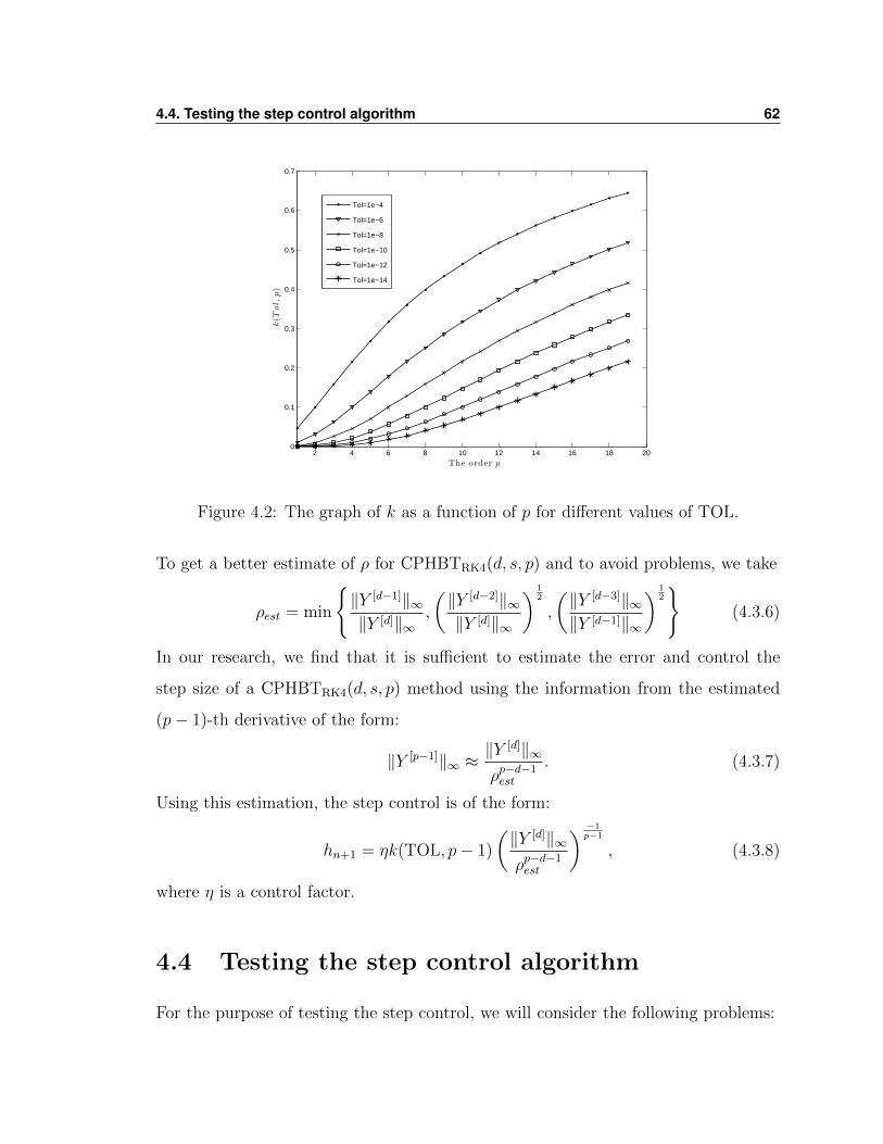
4.4. Testing the step control algorithm 62
2 4 6 8 10 12 14 16 18 200
0.1
0.2
0.3
0.4
0.5
0.6
0.7
The order p
k(T
ol,p)
Tol=1e−4
Tol=1e−6
Tol=1e−8
Tol=1e−10
Tol=1e−12
Tol=1e−14
Figure 4.2: The graph of k as a function of p for different values of TOL.
To get a better estimate of ρ for CPHBTRK4(d, s, p) and to avoid problems, we take
ρest = min
‖Y [d−1]‖∞‖Y [d]‖∞
,
(‖Y [d−2]‖∞‖Y [d]‖∞
) 12
,
(‖Y [d−3]‖∞‖Y [d−1]‖∞
) 12
(4.3.6)
In our research, we find that it is sufficient to estimate the error and control the
step size of a CPHBTRK4(d, s, p) method using the information from the estimated
(p− 1)-th derivative of the form:
‖Y [p−1]‖∞ ≈‖Y [d]‖∞ρp−d−1est
. (4.3.7)
Using this estimation, the step control is of the form:
hn+1 = ηk(TOL, p− 1)
(‖Y [d]‖∞ρp−d−1est
) −1p−1
, (4.3.8)
where η is a control factor.
4.4 Testing the step control algorithm
For the purpose of testing the step control, we will consider the following problems:
4.4. Testing the step control algorithm 63
• HH: The Henon Heiles problem is a well known problem [3, 24] described by
the Hamiltonian:
H =1
2(X2 + Y 2) +
1
2(x2 + y2) + εy(x2 − 1
3y2)
with ε = 1 and the initial values:
x(0) = 0, y(0) = 0.52, X(0) = 0.371956090598519, Y (0) = 0.
• EqMP: The equatorial main problem in the artificial satellite theory [3, 58].
This problem accepts, due to the axial symmetry, the polar component Λ of
the angular momentum as an integral. Other parameters of the problem are
the gravitational constant µ of the planet, the oblateness coefficient J2 and the
scaling factor α that is the equatorial radius of the planet. The Hamiltonian
function in cylindrical coordinates is
H =1
2
(P 2 +
Λ2
ρ2+ Z2
)− µ
r+α2J2µP2(u)
r3,
where u = z/r, r =√ρ2 + z2, and P2(x) = (3x2 − 1)/2 with initial values
ρ(0) = 0.3, z(0) = 2, P (0) = 0 and Z(0) = −1.
The maximum global error (MGE) of a method is taken in the uniform norm
MGE = maxn‖yn − zn‖∞ , (4.4.1)
where yn is the numerical solution and zn is the exact solution at x = xn or a reference
solution obtained by DP(8,7)13M with stringent tolerance 5 × 10⁻¹⁴. This choice
of MGE is ideal to monitor the error uniformly over the whole integration interval
as opposed to the end point error defined by the difference between the numerical
solution and the exact or reference solution at the endpoint of the integration interval
only.
In our numerical simulations, η = 1.4 gave optimal results for CPHBTRK4(9, 6, 12)
in terms of the number of steps required and the difference |TOL −MGE|. In Ta-
ble 4.1, we test the step control algorithm (4.3.8) of CPHBTRK4(9, 6, 12) compared
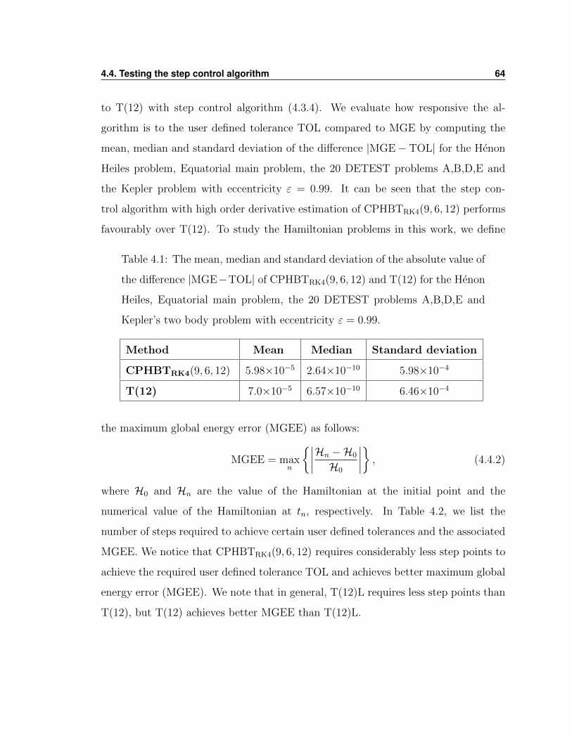
4.4. Testing the step control algorithm 64
to T(12) with step control algorithm (4.3.4). We evaluate how responsive the al-
gorithm is to the user defined tolerance TOL compared to MGE by computing the
mean, median and standard deviation of the difference |MGE− TOL| for the Henon
Heiles problem, Equatorial main problem, the 20 DETEST problems A,B,D,E and
the Kepler problem with eccentricity ε = 0.99. It can be seen that the step con-
trol algorithm with high order derivative estimation of CPHBTRK4(9, 6, 12) performs
favourably over T(12). To study the Hamiltonian problems in this work, we define
Table 4.1: The mean, median and standard deviation of the absolute value of
the difference |MGE−TOL| of CPHBTRK4(9, 6, 12) and T(12) for the Henon
Heiles, Equatorial main problem, the 20 DETEST problems A,B,D,E and
Kepler’s two body problem with eccentricity ε = 0.99.
Method Mean Median Standard deviation
CPHBTRK4(9, 6, 12) 5.98×10⁻⁵ 2.64×10⁻¹⁰ 5.98×10⁻⁴
T(12) 7.0×10⁻⁵ 6.57×10⁻¹⁰ 6.46×10⁻⁴
the maximum global energy error (MGEE) as follows:
MGEE = maxn
∣∣∣∣Hn −H0
H0
∣∣∣∣ , (4.4.2)
where H0 and Hn are the value of the Hamiltonian at the initial point and the
numerical value of the Hamiltonian at tn, respectively. In Table 4.2, we list the
number of steps required to achieve certain user defined tolerances and the associated
MGEE. We notice that CPHBTRK4(9, 6, 12) requires considerably less step points to
achieve the required user defined tolerance TOL and achieves better maximum global
energy error (MGEE). We note that in general, T(12)L requires less step points than
T(12), but T(12) achieves better MGEE than T(12)L.
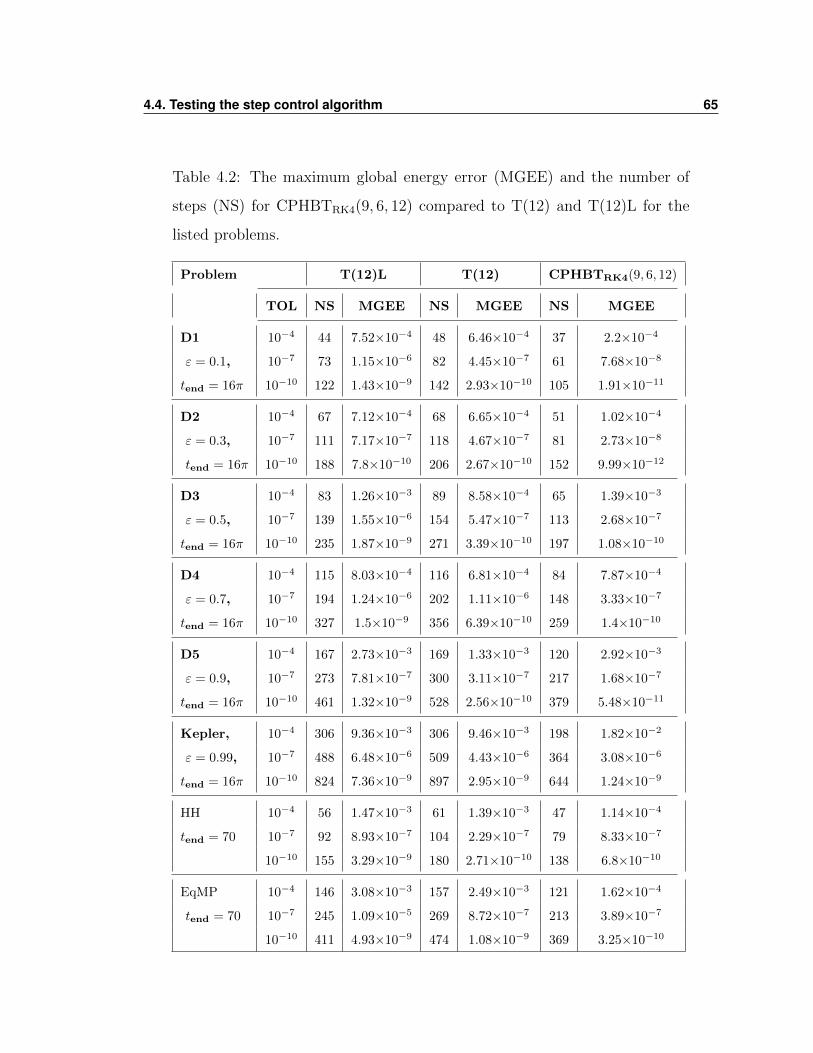
4.4. Testing the step control algorithm 65
Table 4.2: The maximum global energy error (MGEE) and the number of
steps (NS) for CPHBTRK4(9, 6, 12) compared to T(12) and T(12)L for the
listed problems.
Problem T(12)L T(12) CPHBTRK4(9, 6, 12)
TOL NS MGEE NS MGEE NS MGEE
D1 10−4 44 7.52×10⁻⁴ 48 6.46×10⁻⁴ 37 2.2×10⁻⁴
ε = 0.1, 10−7 73 1.15×10⁻⁶ 82 4.45×10⁻⁷ 61 7.68×10⁻⁸
tend = 16π 10−10 122 1.43×10⁻⁹ 142 2.93×10⁻¹⁰ 105 1.91×10⁻¹¹
D2 10−4 67 7.12×10⁻⁴ 68 6.65×10⁻⁴ 51 1.02×10⁻⁴
ε = 0.3, 10−7 111 7.17×10⁻⁷ 118 4.67×10⁻⁷ 81 2.73×10⁻⁸
tend = 16π 10−10 188 7.8×10⁻¹⁰ 206 2.67×10⁻¹⁰ 152 9.99×10⁻¹²
D3 10−4 83 1.26×10⁻³ 89 8.58×10⁻⁴ 65 1.39×10⁻³
ε = 0.5, 10−7 139 1.55×10⁻⁶ 154 5.47×10⁻⁷ 113 2.68×10⁻⁷
tend = 16π 10−10 235 1.87×10⁻⁹ 271 3.39×10⁻¹⁰ 197 1.08×10⁻¹⁰
D4 10−4 115 8.03×10⁻⁴ 116 6.81×10⁻⁴ 84 7.87×10⁻⁴
ε = 0.7, 10−7 194 1.24×10⁻⁶ 202 1.11×10⁻⁶ 148 3.33×10⁻⁷
tend = 16π 10−10 327 1.5×10⁻⁹ 356 6.39×10⁻¹⁰ 259 1.4×10⁻¹⁰
D5 10−4 167 2.73×10⁻³ 169 1.33×10⁻³ 120 2.92×10⁻³
ε = 0.9, 10−7 273 7.81×10⁻⁷ 300 3.11×10⁻⁷ 217 1.68×10⁻⁷
tend = 16π 10−10 461 1.32×10⁻⁹ 528 2.56×10⁻¹⁰ 379 5.48×10⁻¹¹
Kepler, 10−4 306 9.36×10⁻³ 306 9.46×10⁻³ 198 1.82×10⁻²
ε = 0.99, 10−7 488 6.48×10⁻⁶ 509 4.43×10⁻⁶ 364 3.08×10⁻⁶
tend = 16π 10−10 824 7.36×10⁻⁹ 897 2.95×10⁻⁹ 644 1.24×10⁻⁹
HH 10−4 56 1.47×10⁻³ 61 1.39×10⁻³ 47 1.14×10⁻⁴
tend = 70 10−7 92 8.93×10⁻⁷ 104 2.29×10⁻⁷ 79 8.33×10⁻⁷
10−10 155 3.29×10⁻⁹ 180 2.71×10⁻¹⁰ 138 6.8×10⁻¹⁰
EqMP 10−4 146 3.08×10⁻³ 157 2.49×10⁻³ 121 1.62×10⁻⁴
tend = 70 10−7 245 1.09×10⁻⁵ 269 8.72×10⁻⁷ 213 3.89×10⁻⁷
10−10 411 4.93×10⁻⁹ 474 1.08×10⁻⁹ 369 3.25×10⁻¹⁰
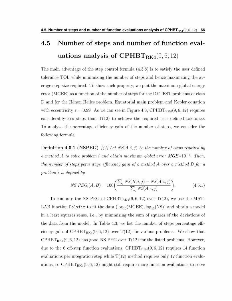
4.5. Number of steps and number of function evaluations analysis of CPHBTRK4(9, 6, 12) 66
4.5 Number of steps and number of function eval-
uations analysis of CPHBTRK4(9, 6, 12)
The main advantage of the step control formula (4.3.8) is to satisfy the user defined
tolerance TOL while minimizing the number of steps and hence maximizing the av-
erage step-size required. To show such property, we plot the maximum global energy
error (MGEE) as a function of the number of steps for the DETEST problems of class
D and for the Henon Heiles problem, Equatorial main problem and Kepler equation
with eccentricity ε = 0.99. As we can see in Figure 4.3, CPHBTRK4(9, 6, 12) requires
considerably less steps than T(12) to achieve the required user defined tolerance.
To analyze the percentage efficiency gain of the number of steps, we consider the
following formula:
Definition 4.5.1 (NSPEG) [41] Let NS(A, i, j) be the number of steps required by
a method A to solve problem i and obtain maximum global error MGE=10−j. Then,
the number of steps percentage efficiency gain of a method A over a method B for a
problem i is defined by
NS PEGi(A,B) = 100
(∑j NS(B, i, j)− NS(A, i, j)∑
j NS(A, i, j)
). (4.5.1)
To compute the NS PEG of CPHBTRK4(9, 6, 12) over T(12), we use the MAT-
LAB function Polyfit to fit the data (log10(MGEE), log10(NS)) and obtain a model
in a least squares sense, i.e., by minimizing the sum of squares of the deviations of
the data from the model. In Table 4.3, we list the number of steps percentage effi-
ciency gain of CPHBTRK4(9, 6, 12) over T(12) for various problems. We show that
CPHBTRK4(9, 6, 12) has good NS PEG over T(12) for the listed problems. However,
due to the 6 off-step function evaluations, CPHBTRK4(9, 6, 12) requires 14 function
evaluations per integration step while T(12) method requires only 12 function evalu-
ations, so CPHBTRK4(9, 6, 12) might still require more function evaluations to solve
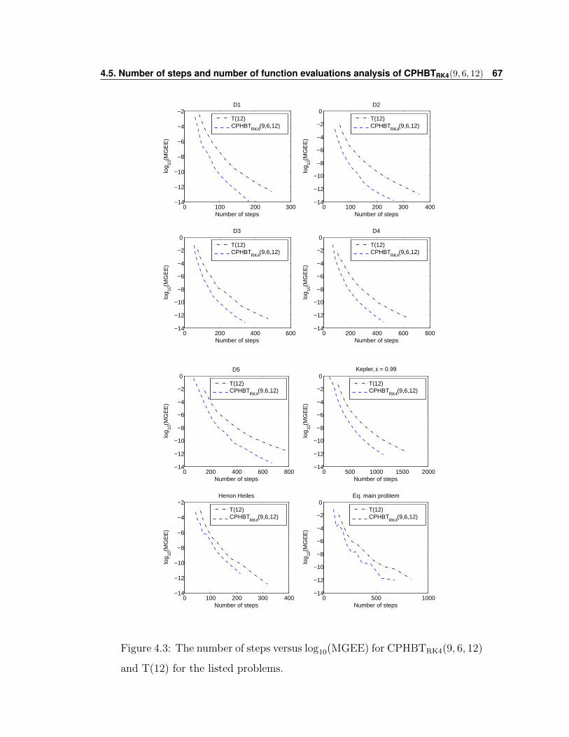
4.5. Number of steps and number of function evaluations analysis of CPHBTRK4(9, 6, 12) 67
0 100 200 300−14
−12
−10
−8
−6
−4
−2D1
Number of steps
log 10
(MG
EE
)
0 100 200 300 400−14
−12
−10
−8
−6
−4
−2
0D2
Number of steps
log 10
(MG
EE
)
0 200 400 600−14
−12
−10
−8
−6
−4
−2
0D3
Number of steps
log 10
(MG
EE
)
0 200 400 600 800−14
−12
−10
−8
−6
−4
−2
0D4
Number of steps
log 10
(MG
EE
)
T(12)CPHBT
RK4(9,6,12)
T(12)CPHBT
RK4(9,6,12)
T(12)CPHBT
RK4(9,6,12)
T(12)CPHBT
RK4(9,6,12)
0 200 400 600 800−14
−12
−10
−8
−6
−4
−2
0D5
Number of steps
log 10
(MG
EE
)
0 500 1000 1500 2000−14
−12
−10
−8
−6
−4
−2
0Kepler, ε = 0.99
Number of steps
log 10
(MG
EE
)
0 100 200 300 400−14
−12
−10
−8
−6
−4
−2Henon Heiles
Number of steps
log 10
(MG
EE
)
0 500 1000−14
−12
−10
−8
−6
−4
−2
0Eq. main problem
Number of steps
log 10
(MG
EE
)
T(12)CPHBT
RK4(9,6,12)
T(12)CPHBT
RK4(9,6,12)
T(12)CPHBT
RK4(9,6,12)
T(12)CPHBT
RK4(9,6,12)
Figure 4.3: The number of steps versus log10(MGEE) for CPHBTRK4(9, 6, 12)
and T(12) for the listed problems.
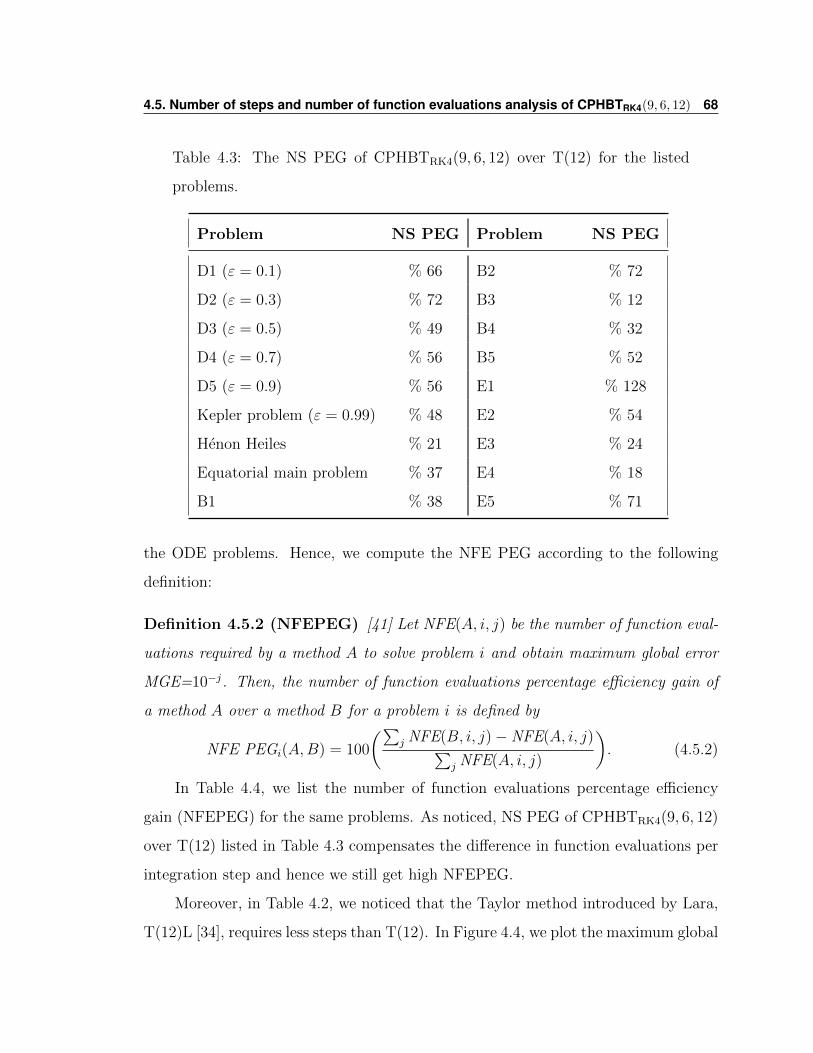
4.5. Number of steps and number of function evaluations analysis of CPHBTRK4(9, 6, 12) 68
Table 4.3: The NS PEG of CPHBTRK4(9, 6, 12) over T(12) for the listed
problems.
Problem NS PEG Problem NS PEG
D1 (ε = 0.1) % 66 B2 % 72
D2 (ε = 0.3) % 72 B3 % 12
D3 (ε = 0.5) % 49 B4 % 32
D4 (ε = 0.7) % 56 B5 % 52
D5 (ε = 0.9) % 56 E1 % 128
Kepler problem (ε = 0.99) % 48 E2 % 54
Henon Heiles % 21 E3 % 24
Equatorial main problem % 37 E4 % 18
B1 % 38 E5 % 71
the ODE problems. Hence, we compute the NFE PEG according to the following
definition:
Definition 4.5.2 (NFEPEG) [41] Let NFE(A, i, j) be the number of function eval-
uations required by a method A to solve problem i and obtain maximum global error
MGE=10−j. Then, the number of function evaluations percentage efficiency gain of
a method A over a method B for a problem i is defined by
NFE PEGi(A,B) = 100
(∑j NFE(B, i, j)− NFE(A, i, j)∑
j NFE(A, i, j)
). (4.5.2)
In Table 4.4, we list the number of function evaluations percentage efficiency
gain (NFEPEG) for the same problems. As noticed, NS PEG of CPHBTRK4(9, 6, 12)
over T(12) listed in Table 4.3 compensates the difference in function evaluations per
integration step and hence we still get high NFEPEG.
Moreover, in Table 4.2, we noticed that the Taylor method introduced by Lara,
T(12)L [34], requires less steps than T(12). In Figure 4.4, we plot the maximum global
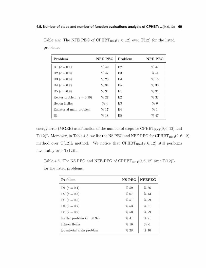
4.5. Number of steps and number of function evaluations analysis of CPHBTRK4(9, 6, 12) 69
Table 4.4: The NFE PEG of CPHBTRK4(9, 6, 12) over T(12) for the listed
problems.
Problem NFE PEG Problem NFE PEG
D1 (ε = 0.1) % 42 B2 % 47
D2 (ε = 0.3) % 47 B3 % -4
D3 (ε = 0.5) % 28 B4 % 13
D4 (ε = 0.7) % 34 B5 % 30
D5 (ε = 0.9) % 34 E1 % 95
Kepler problem (ε = 0.99) % 27 E2 % 32
Henon Heiles % 4 E3 % 6
Equatorial main problem % 17 E4 % 1
B1 % 18 E5 % 47
energy error (MGEE) as a function of the number of steps for CPHBTRK4(9, 6, 12) and
T(12)L. Moreover, in Table 4.5, we list the NS PEG and NFE PEG for CPHBTRK4(9, 6, 12)
method over T(12)L method. We notice that CPHBTRK4(9, 6, 12) still performs
favourably over T(12)L.
Table 4.5: The NS PEG and NFE PEG of CPHBTRK4(9, 6, 12) over T(12)L
for the listed problems.
Problem NS PEG NFEPEG
D1 (ε = 0.1) % 59 % 36
D2 (ε = 0.3) % 67 % 43
D3 (ε = 0.5) % 51 % 29
D4 (ε = 0.7) % 53 % 31
D5 (ε = 0.9) % 50 % 29
Kepler problem (ε = 0.99) % 41 % 21
Henon Heiles % 16 % -1
Equatorial main problem % 28 % 10
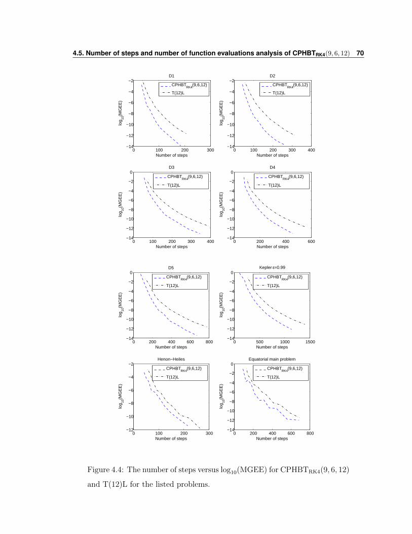
4.5. Number of steps and number of function evaluations analysis of CPHBTRK4(9, 6, 12) 70
0 100 200 300−14
−12
−10
−8
−6
−4
−2
Number of steps
log 10
(MG
EE
)
D1
CPHBT
RK4(9,6,12)
T(12)L
0 100 200 300 400−14
−12
−10
−8
−6
−4
−2
Number of steps
log 10
(MG
EE
)
D2
CPHBT
RK4(9,6,12)
T(12)L
0 100 200 300 400−14
−12
−10
−8
−6
−4
−2
0
Number of steps
log 10
(MG
EE
)
D3
CPHBT
RK4(9,6,12)
T(12)L
0 200 400 600−14
−12
−10
−8
−6
−4
−2
0
Number of steps
log 10
(MG
EE
)
D4
CPHBT
RK4(9,6,12)
T(12)L
0 200 400 600 800−14
−12
−10
−8
−6
−4
−2
0
Number of steps
log 10
(MG
EE
)
D5
CPHBT
RK4(9,6,12)
T(12)L
0 500 1000 1500−14
−12
−10
−8
−6
−4
−2
0
Number of steps
log 10
(MG
EE
)
Kepler ε=0.99
CPHBT
RK4(9,6,12)
T(12)L
0 100 200 300−12
−10
−8
−6
−4
−2
Number of steps
log 10
(MG
EE
)
Henon−Heiles
CPHBT
RK4(9,6,12)
T(12)L
0 200 400 600 800−14
−12
−10
−8
−6
−4
−2
0
Number of steps
log 10
(MG
EE
)
Equatorial main problem
CPHBT
RK4(9,6,12)
T(12)L
Figure 4.4: The number of steps versus log10(MGEE) for CPHBTRK4(9, 6, 12)
and T(12)L for the listed problems.
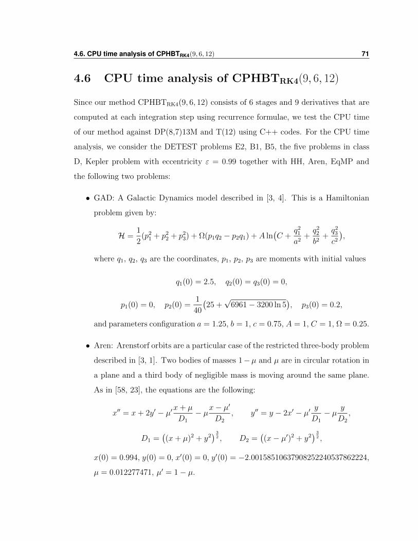
4.6. CPU time analysis of CPHBTRK4(9, 6, 12) 71
4.6 CPU time analysis of CPHBTRK4(9, 6, 12)
Since our method CPHBTRK4(9, 6, 12) consists of 6 stages and 9 derivatives that are
computed at each integration step using recurrence formulae, we test the CPU time
of our method against DP(8,7)13M and T(12) using C++ codes. For the CPU time
analysis, we consider the DETEST problems E2, B1, B5, the five problems in class
D, Kepler problem with eccentricity ε = 0.99 together with HH, Aren, EqMP and
the following two problems:
• GAD: A Galactic Dynamics model described in [3, 4]. This is a Hamiltonian
problem given by:
H =1
2(p2
1 + p22 + p2
3) + Ω(p1q2 − p2q1) + A ln(C +
q21
a2+q2
2
b2+q2
3
c2
),
where q1, q2, q3 are the coordinates, p1, p2, p3 are moments with initial values
q1(0) = 2.5, q2(0) = q3(0) = 0,
p1(0) = 0, p2(0) =1
40
(25 +
√6961− 3200 ln 5
), p3(0) = 0.2,
and parameters configuration a = 1.25, b = 1, c = 0.75, A = 1, C = 1, Ω = 0.25.
• Aren: Arenstorf orbits are a particular case of the restricted three-body problem
described in [3, 1]. Two bodies of masses 1−µ and µ are in circular rotation in
a plane and a third body of negligible mass is moving around the same plane.
As in [58, 23], the equations are the following:
x′′ = x+ 2y′ − µ′x+ µ
D1
− µx− µ′
D2
, y′′ = y − 2x′ − µ′ yD1
− µ y
D2
,
D1 =((x+ µ)2 + y2
) 32 , D2 =
((x− µ′)2 + y2
) 32 ,
x(0) = 0.994, y(0) = 0, x′(0) = 0, y′(0) = −2.00158510637908252240537862224,
µ = 0.012277471, µ′ = 1− µ.
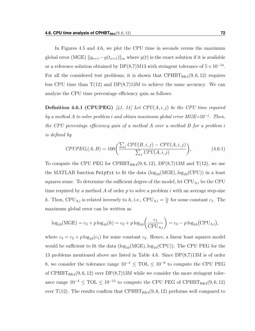
4.6. CPU time analysis of CPHBTRK4(9, 6, 12) 72
In Figures 4.5 and 4.6, we plot the CPU time in seconds versus the maximum
global error (MGE) ‖yn+1−y(tn+1)‖∞ where y(t) is the exact solution if it is available
or a reference solution obtained by DP(8,7)M13 with stringent tolerance of 5×10⁻¹⁴.
For all the considered test problems, it is shown that CPHBTRK4(9, 6, 12) requires
less CPU time than T(12) and DP(8,7)13M to achieve the same accuracy. We can
analyze the CPU time percentage efficiency gain as follows:
Definition 4.6.1 (CPUPEG) [41, 51] Let CPU(A, i, j) be the CPU time required
by a method A to solve problem i and obtain maximum global error MGE=10−j. Then,
the CPU percentage efficiency gain of a method A over a method B for a problem i
is defined by
CPUPEGi(A,B) = 100
(∑j CPU(B, i, j)− CPU(A, i, j)∑
j CPU(A, i, j)
), (4.6.1)
To compute the CPU PEG for CPHBTRK4(9, 6, 12), DP(8,7)13M and T(12), we use
the MATLAB function Polyfit to fit the data (log10(MGE), log10(CPU)) in a least
squares sense. To determine the sufficient degree of the model, let CPUA,i be the CPU
time required by a method A of order p to solve a problem i with an average step-size
h. Then, CPUA,i is related inversely to h, i.e., CPUA,i = c1h
for some constant c1. The
maximum global error can be written as
log10(MGE) = c2 + p log10(h) = c2 + p log10
(c1
CPUA,i
)= c3 − p log10
(CPUA,i
),
where c3 = c2 + p log10(c1) for some constant c2. Hence, a linear least squares model
would be sufficient to fit the data (log10(MGE), log10(CPU)). The CPU PEG for the
13 problems mentioned above are listed in Table 4.6. Since DP(8,7)13M is of order
8, we consider the tolerance range 10−4 ≤ TOL ≤ 10−9 to compute the CPU PEG
of CPHBTRK4(9, 6, 12) over DP(8,7)13M while we consider the more stringent toler-
ance range 10−4 ≤ TOL ≤ 10−13 to compute the CPU PEG of CPHBTRK4(9, 6, 12)
over T(12). The results confirm that CPHBTRK4(9, 6, 12) performs well compared to
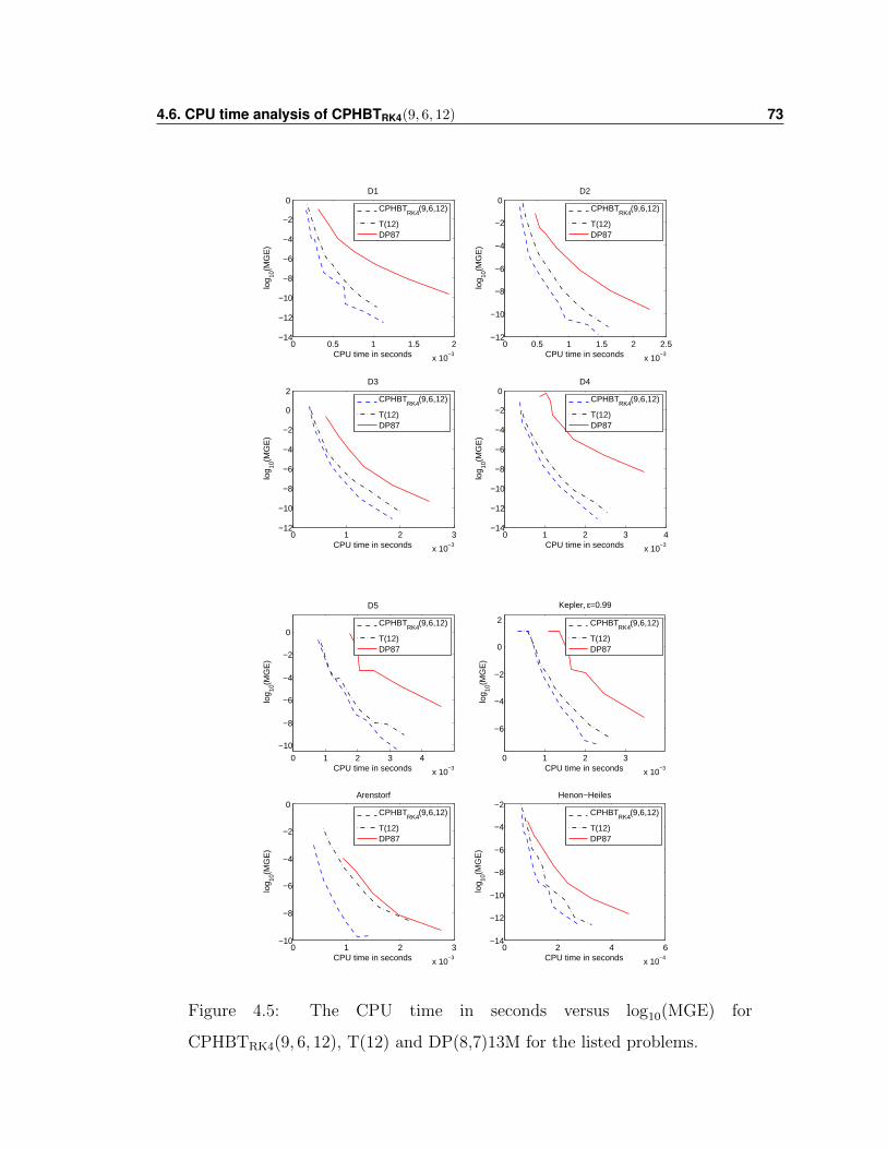
4.6. CPU time analysis of CPHBTRK4(9, 6, 12) 73
0 0.5 1 1.5 2
x 10−3
−14
−12
−10
−8
−6
−4
−2
0
log 10
(MG
E)
CPU time in seconds
D1
CPHBT
RK4(9,6,12)
T(12)DP87
0 0.5 1 1.5 2 2.5
x 10−3
−12
−10
−8
−6
−4
−2
0
log 10
(MG
E)
CPU time in seconds
D2
CPHBT
RK4(9,6,12)
T(12)DP87
0 1 2 3
x 10−3
−12
−10
−8
−6
−4
−2
0
2
log 10
(MG
E)
CPU time in seconds
D3
CPHBT
RK4(9,6,12)
T(12)DP87
0 1 2 3 4
x 10−3
−14
−12
−10
−8
−6
−4
−2
0
log 10
(MG
E)
CPU time in seconds
D4
CPHBT
RK4(9,6,12)
T(12)DP87
0 1 2 3 4
x 10−3
−10
−8
−6
−4
−2
0
log 10
(MG
E)
CPU time in seconds
D5
CPHBT
RK4(9,6,12)
T(12)DP87
0 1 2 3
x 10−3
−6
−4
−2
0
2
log 10
(MG
E)
CPU time in seconds
Kepler, ε=0.99
CPHBT
RK4(9,6,12)
T(12)DP87
0 1 2 3
x 10−3
−10
−8
−6
−4
−2
0
log 10
(MG
E)
CPU time in seconds
Arenstorf
CPHBT
RK4(9,6,12)
T(12)DP87
0 2 4 6
x 10−4
−14
−12
−10
−8
−6
−4
−2
log 10
(MG
E)
CPU time in seconds
Henon−Heiles
CPHBT
RK4(9,6,12)
T(12)DP87
Figure 4.5: The CPU time in seconds versus log10(MGE) for
CPHBTRK4(9, 6, 12), T(12) and DP(8,7)13M for the listed problems.
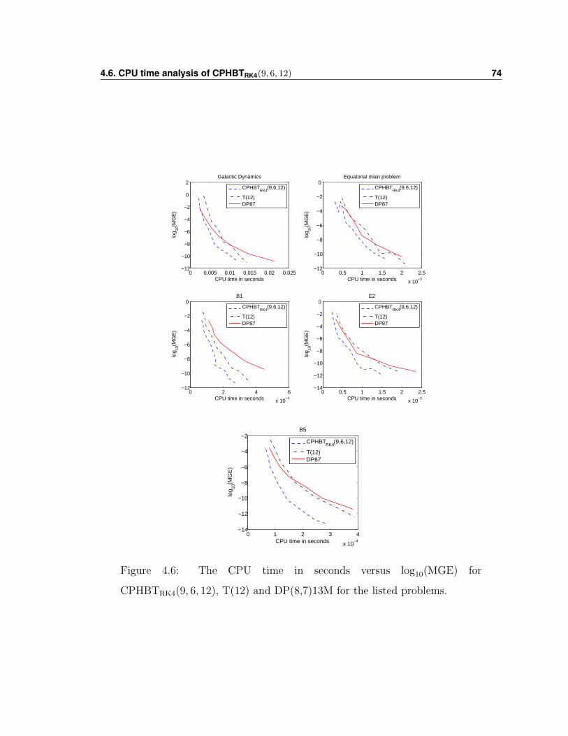
4.6. CPU time analysis of CPHBTRK4(9, 6, 12) 74
0 0.005 0.01 0.015 0.02 0.025−12
−10
−8
−6
−4
−2
0
2
log 10
(MG
E)
CPU time in seconds
Galactic Dynamics
CPHBT
RK4(9,6,12)
T(12)DP87
0 0.5 1 1.5 2 2.5
x 10−3
−12
−10
−8
−6
−4
−2
0
log 10
(MG
E)
CPU time in seconds
Equatorial main problem
CPHBT
RK4(9,6,12)
T(12)DP87
0 2 4 6
x 10−4
−12
−10
−8
−6
−4
−2
0
log 10
(MG
E)
CPU time in seconds
B1
CPHBT
RK4(9,6,12)
T(12)DP87
0 0.5 1 1.5 2 2.5
x 10−3
−14
−12
−10
−8
−6
−4
−2
0lo
g 10(M
GE
)
CPU time in seconds
E2
CPHBT
RK4(9,6,12)
T(12)DP87
0 1 2 3 4
x 10−4
−14
−12
−10
−8
−6
−4
−2
log 10
(MG
E)
CPU time in seconds
B5
CPHBT
RK4(9,6,12)
T(12)DP87
Figure 4.6: The CPU time in seconds versus log10(MGE) for
CPHBTRK4(9, 6, 12), T(12) and DP(8,7)13M for the listed problems.
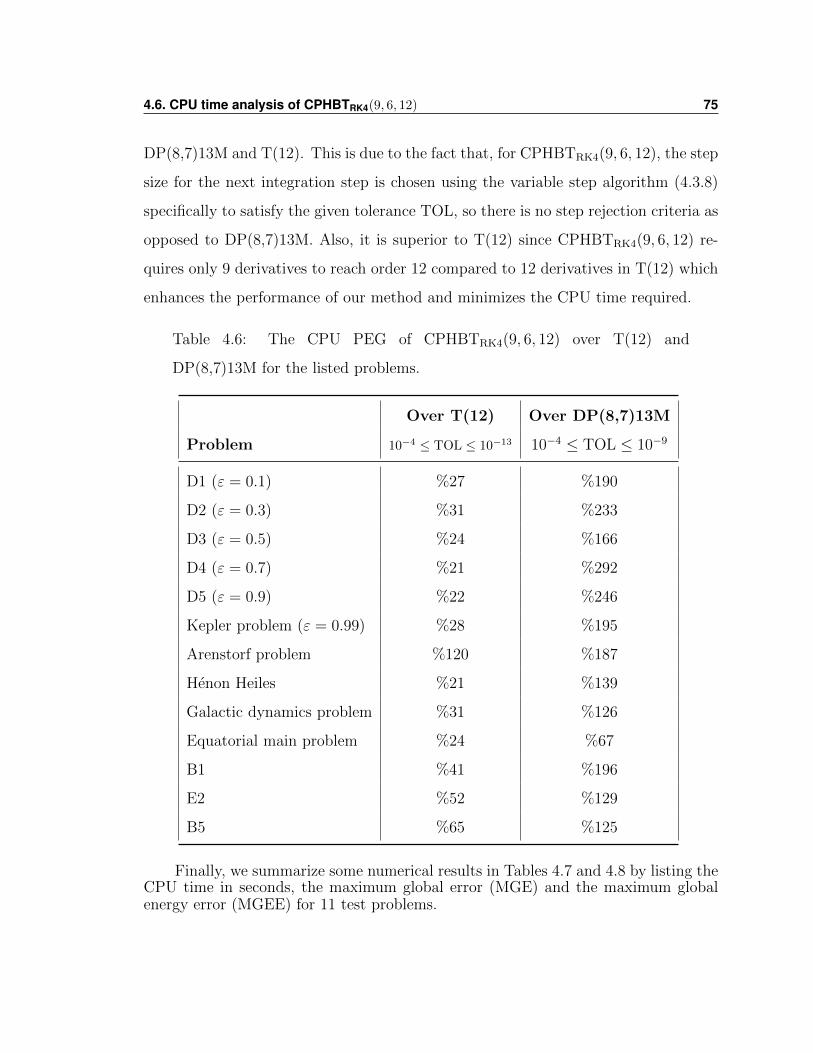
4.6. CPU time analysis of CPHBTRK4(9, 6, 12) 75
DP(8,7)13M and T(12). This is due to the fact that, for CPHBTRK4(9, 6, 12), the step
size for the next integration step is chosen using the variable step algorithm (4.3.8)
specifically to satisfy the given tolerance TOL, so there is no step rejection criteria as
opposed to DP(8,7)13M. Also, it is superior to T(12) since CPHBTRK4(9, 6, 12) re-
quires only 9 derivatives to reach order 12 compared to 12 derivatives in T(12) which
enhances the performance of our method and minimizes the CPU time required.
Table 4.6: The CPU PEG of CPHBTRK4(9, 6, 12) over T(12) and
DP(8,7)13M for the listed problems.
Over T(12) Over DP(8,7)13M
Problem 10−4 ≤ TOL ≤ 10−13 10−4 ≤ TOL ≤ 10−9
D1 (ε = 0.1) %27 %190
D2 (ε = 0.3) %31 %233
D3 (ε = 0.5) %24 %166
D4 (ε = 0.7) %21 %292
D5 (ε = 0.9) %22 %246
Kepler problem (ε = 0.99) %28 %195
Arenstorf problem %120 %187
Henon Heiles %21 %139
Galactic dynamics problem %31 %126
Equatorial main problem %24 %67
B1 %41 %196
E2 %52 %129
B5 %65 %125
Finally, we summarize some numerical results in Tables 4.7 and 4.8 by listing theCPU time in seconds, the maximum global error (MGE) and the maximum globalenergy error (MGEE) for 11 test problems.
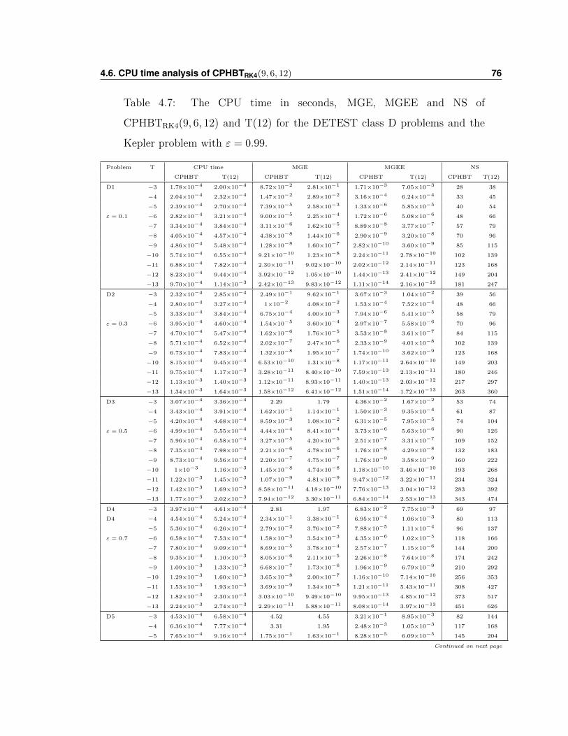
4.6. CPU time analysis of CPHBTRK4(9, 6, 12) 76
Table 4.7: The CPU time in seconds, MGE, MGEE and NS of
CPHBTRK4(9, 6, 12) and T(12) for the DETEST class D problems and the
Kepler problem with ε = 0.99.
Problem T CPU time MGE MGEE NS
CPHBT T(12) CPHBT T(12) CPHBT T(12) CPHBT T(12)
D1 −3 1.78×10⁻⁴ 2.00×10⁻⁴ 8.72×10⁻² 2.81×10⁻¹ 1.71×10⁻³ 7.05×10⁻³ 28 38
−4 2.04×10⁻⁴ 2.32×10⁻⁴ 1.47×10⁻² 2.89×10⁻² 3.16×10⁻⁴ 6.24×10⁻⁴ 33 45
−5 2.39×10⁻⁴ 2.70×10⁻⁴ 7.39×10⁻⁵ 2.58×10⁻³ 1.33×10⁻⁶ 5.85×10⁻⁵ 40 54
ε = 0.1 −6 2.82×10⁻⁴ 3.21×10⁻⁴ 9.00×10⁻⁵ 2.25×10⁻⁴ 1.72×10⁻⁶ 5.08×10⁻⁶ 48 66
−7 3.34×10⁻⁴ 3.84×10⁻⁴ 3.11×10⁻⁶ 1.62×10⁻⁵ 8.89×10⁻⁸ 3.77×10⁻⁷ 57 79
−8 4.05×10⁻⁴ 4.57×10⁻⁴ 4.38×10⁻⁸ 1.44×10⁻⁶ 2.90×10⁻⁹ 3.20×10⁻⁸ 70 96
−9 4.86×10⁻⁴ 5.48×10⁻⁴ 1.28×10⁻⁸ 1.60×10⁻⁷ 2.82×10⁻¹⁰ 3.60×10⁻⁹ 85 115
−10 5.74×10⁻⁴ 6.55×10⁻⁴ 9.21×10⁻¹⁰ 1.23×10⁻⁸ 2.24×10⁻¹¹ 2.78×10⁻¹⁰ 102 139
−11 6.88×10⁻⁴ 7.82×10⁻⁴ 2.30×10⁻¹¹ 9.02×10⁻¹⁰ 2.02×10⁻¹² 2.14×10⁻¹¹ 123 168
−12 8.23×10⁻⁴ 9.44×10⁻⁴ 3.92×10⁻¹² 1.05×10⁻¹⁰ 1.44×10⁻¹³ 2.41×10⁻¹² 149 204
−13 9.70×10⁻⁴ 1.14×10⁻³ 2.42×10⁻¹³ 9.83×10⁻¹² 1.11×10⁻¹⁴ 2.16×10⁻¹³ 181 247
D2 −3 2.32×10⁻⁴ 2.85×10⁻⁴ 2.49×10⁻¹ 9.62×10⁻¹ 3.67×10⁻³ 1.04×10⁻² 39 56
−4 2.80×10⁻⁴ 3.27×10⁻⁴ 1×10⁻² 4.08×10⁻² 1.53×10⁻⁴ 7.52×10⁻⁴ 48 66
−5 3.33×10⁻⁴ 3.84×10⁻⁴ 6.75×10⁻⁴ 4.00×10⁻³ 7.94×10⁻⁶ 5.41×10⁻⁵ 58 79
ε = 0.3 −6 3.95×10⁻⁴ 4.60×10⁻⁴ 1.54×10⁻⁵ 3.60×10⁻⁴ 2.97×10⁻⁷ 5.58×10⁻⁶ 70 96
−7 4.70×10⁻⁴ 5.47×10⁻⁴ 1.62×10⁻⁶ 1.76×10⁻⁵ 3.53×10⁻⁸ 3.61×10⁻⁷ 84 115
−8 5.71×10⁻⁴ 6.52×10⁻⁴ 2.02×10⁻⁷ 2.47×10⁻⁶ 2.33×10⁻⁹ 4.01×10⁻⁸ 102 139
−9 6.73×10⁻⁴ 7.83×10⁻⁴ 1.32×10⁻⁸ 1.95×10⁻⁷ 1.74×10⁻¹⁰ 3.62×10⁻⁹ 123 168
−10 8.15×10⁻⁴ 9.45×10⁻⁴ 6.53×10⁻¹⁰ 1.31×10⁻⁸ 1.17×10⁻¹¹ 2.64×10⁻¹⁰ 149 203
−11 9.75×10⁻⁴ 1.17×10⁻³ 3.28×10⁻¹¹ 8.40×10⁻¹⁰ 7.59×10⁻¹³ 2.13×10⁻¹¹ 180 246
−12 1.13×10⁻³ 1.40×10⁻³ 1.12×10⁻¹¹ 8.93×10⁻¹¹ 1.40×10⁻¹³ 2.03×10⁻¹² 217 297
−13 1.34×10⁻³ 1.64×10⁻³ 1.58×10⁻¹² 6.41×10⁻¹² 1.51×10⁻¹⁴ 1.72×10⁻¹³ 263 360
D3 −3 3.07×10⁻⁴ 3.36×10⁻⁴ 2.29 1.79 4.36×10⁻² 1.67×10⁻² 53 74
−4 3.43×10⁻⁴ 3.91×10⁻⁴ 1.62×10⁻¹ 1.14×10⁻¹ 1.50×10⁻³ 9.35×10⁻⁴ 61 87
−5 4.20×10⁻⁴ 4.68×10⁻⁴ 8.59×10⁻³ 1.08×10⁻² 6.31×10⁻⁵ 7.95×10⁻⁵ 74 104
ε = 0.5 −6 4.99×10⁻⁴ 5.55×10⁻⁴ 4.44×10⁻⁴ 8.41×10⁻⁴ 3.73×10⁻⁶ 5.63×10⁻⁶ 90 126
−7 5.96×10⁻⁴ 6.58×10⁻⁴ 3.27×10⁻⁵ 4.20×10⁻⁵ 2.51×10⁻⁷ 3.31×10⁻⁷ 109 152
−8 7.35×10⁻⁴ 7.98×10⁻⁴ 2.21×10⁻⁶ 4.78×10⁻⁶ 1.76×10⁻⁸ 4.29×10⁻⁸ 132 183
−9 8.73×10⁻⁴ 9.56×10⁻⁴ 2.20×10⁻⁷ 4.75×10⁻⁷ 1.76×10⁻⁹ 3.58×10⁻⁹ 160 222
−10 1×10⁻³ 1.16×10⁻³ 1.45×10⁻⁸ 4.74×10⁻⁸ 1.18×10⁻¹⁰ 3.46×10⁻¹⁰ 193 268
−11 1.22×10⁻³ 1.45×10⁻³ 1.07×10⁻⁹ 4.81×10⁻⁹ 9.47×10⁻¹² 3.22×10⁻¹¹ 234 324
−12 1.42×10⁻³ 1.69×10⁻³ 8.58×10⁻¹¹ 4.18×10⁻¹⁰ 7.76×10⁻¹³ 3.04×10⁻¹² 283 392
−13 1.77×10⁻³ 2.02×10⁻³ 7.94×10⁻¹² 3.30×10⁻¹¹ 6.84×10⁻¹⁴ 2.53×10⁻¹³ 343 474
D4 −3 3.97×10⁻⁴ 4.61×10⁻⁴ 2.81 1.97 6.83×10⁻² 7.75×10⁻³ 69 97
D4 −4 4.54×10⁻⁴ 5.24×10⁻⁴ 2.34×10⁻¹ 3.38×10⁻¹ 6.95×10⁻⁴ 1.06×10⁻³ 80 113
−5 5.36×10⁻⁴ 6.26×10⁻⁴ 2.79×10⁻² 3.76×10⁻² 7.88×10⁻⁵ 1.11×10⁻⁴ 96 137
ε = 0.7 −6 6.58×10⁻⁴ 7.53×10⁻⁴ 1.58×10⁻³ 3.54×10⁻³ 4.35×10⁻⁶ 1.02×10⁻⁵ 118 166
−7 7.80×10⁻⁴ 9.09×10⁻⁴ 8.69×10⁻⁵ 3.78×10⁻⁴ 2.57×10⁻⁷ 1.15×10⁻⁶ 144 200
−8 9.35×10⁻⁴ 1.10×10⁻³ 8.05×10⁻⁶ 2.11×10⁻⁵ 2.26×10⁻⁸ 7.64×10⁻⁸ 174 242
−9 1.09×10⁻³ 1.33×10⁻³ 6.68×10⁻⁷ 1.73×10⁻⁶ 1.96×10⁻⁹ 6.79×10⁻⁹ 210 292
−10 1.29×10⁻³ 1.60×10⁻³ 3.65×10⁻⁸ 2.00×10⁻⁷ 1.16×10⁻¹⁰ 7.14×10⁻¹⁰ 256 353
−11 1.53×10⁻³ 1.93×10⁻³ 3.69×10⁻⁹ 1.34×10⁻⁸ 1.21×10⁻¹¹ 5.43×10⁻¹¹ 308 427
−12 1.82×10⁻³ 2.30×10⁻³ 3.03×10⁻¹⁰ 9.49×10⁻¹⁰ 9.95×10⁻¹³ 4.85×10⁻¹² 373 517
−13 2.24×10⁻³ 2.74×10⁻³ 2.29×10⁻¹¹ 5.88×10⁻¹¹ 8.08×10⁻¹⁴ 3.97×10⁻¹³ 451 626
D5 −3 4.53×10⁻⁴ 6.58×10⁻⁴ 4.52 4.55 3.21×10⁻¹ 8.95×10⁻³ 82 144
−4 6.36×10⁻⁴ 7.77×10⁻⁴ 3.31 1.95 2.48×10⁻³ 1.05×10⁻³ 117 168
−5 7.65×10⁻⁴ 9.16×10⁻⁴ 1.75×10⁻¹ 1.63×10⁻¹ 8.28×10⁻⁵ 6.09×10⁻⁵ 145 204
Continued on next page
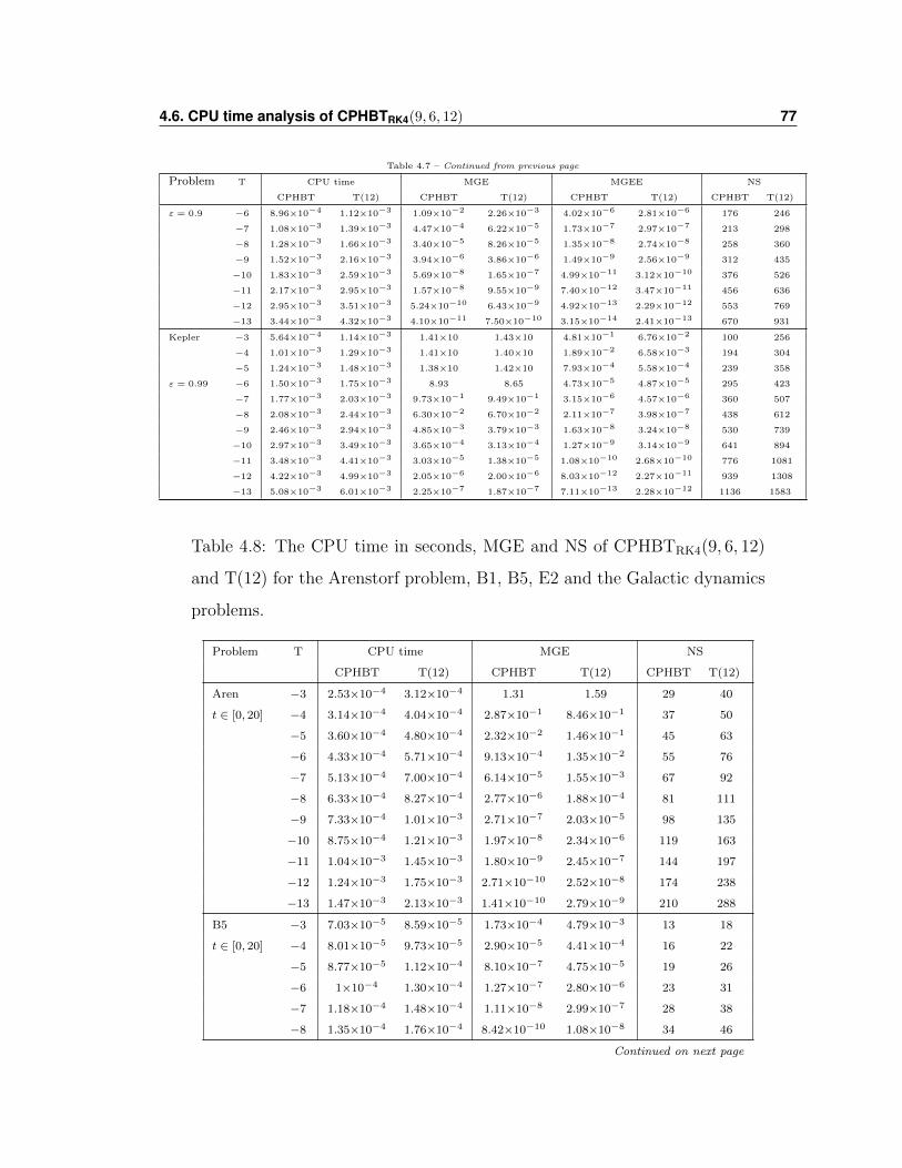
4.6. CPU time analysis of CPHBTRK4(9, 6, 12) 77
Table 4.7 – Continued from previous page
Problem T CPU time MGE MGEE NS
CPHBT T(12) CPHBT T(12) CPHBT T(12) CPHBT T(12)
ε = 0.9 −6 8.96×10⁻⁴ 1.12×10⁻³ 1.09×10⁻² 2.26×10⁻³ 4.02×10⁻⁶ 2.81×10⁻⁶ 176 246
−7 1.08×10⁻³ 1.39×10⁻³ 4.47×10⁻⁴ 6.22×10⁻⁵ 1.73×10⁻⁷ 2.97×10⁻⁷ 213 298
−8 1.28×10⁻³ 1.66×10⁻³ 3.40×10⁻⁵ 8.26×10⁻⁵ 1.35×10⁻⁸ 2.74×10⁻⁸ 258 360
−9 1.52×10⁻³ 2.16×10⁻³ 3.94×10⁻⁶ 3.86×10⁻⁶ 1.49×10⁻⁹ 2.56×10⁻⁹ 312 435
−10 1.83×10⁻³ 2.59×10⁻³ 5.69×10⁻⁸ 1.65×10⁻⁷ 4.99×10⁻¹¹ 3.12×10⁻¹⁰ 376 526
−11 2.17×10⁻³ 2.95×10⁻³ 1.57×10⁻⁸ 9.55×10⁻⁹ 7.40×10⁻¹² 3.47×10⁻¹¹ 456 636
−12 2.95×10⁻³ 3.51×10⁻³ 5.24×10⁻¹⁰ 6.43×10⁻⁹ 4.92×10⁻¹³ 2.29×10⁻¹² 553 769
−13 3.44×10⁻³ 4.32×10⁻³ 4.10×10⁻¹¹ 7.50×10⁻¹⁰ 3.15×10⁻¹⁴ 2.41×10⁻¹³ 670 931
Kepler −3 5.64×10⁻⁴ 1.14×10⁻³ 1.41×10 1.43×10 4.81×10⁻¹ 6.76×10⁻² 100 256
−4 1.01×10⁻³ 1.29×10⁻³ 1.41×10 1.40×10 1.89×10⁻² 6.58×10⁻³ 194 304
−5 1.24×10⁻³ 1.48×10⁻³ 1.38×10 1.42×10 7.93×10⁻⁴ 5.58×10⁻⁴ 239 358
ε = 0.99 −6 1.50×10⁻³ 1.75×10⁻³ 8.93 8.65 4.73×10⁻⁵ 4.87×10⁻⁵ 295 423
−7 1.77×10⁻³ 2.03×10⁻³ 9.73×10⁻¹ 9.49×10⁻¹ 3.15×10⁻⁶ 4.57×10⁻⁶ 360 507
−8 2.08×10⁻³ 2.44×10⁻³ 6.30×10⁻² 6.70×10⁻² 2.11×10⁻⁷ 3.98×10⁻⁷ 438 612
−9 2.46×10⁻³ 2.94×10⁻³ 4.85×10⁻³ 3.79×10⁻³ 1.63×10⁻⁸ 3.24×10⁻⁸ 530 739
−10 2.97×10⁻³ 3.49×10⁻³ 3.65×10⁻⁴ 3.13×10⁻⁴ 1.27×10⁻⁹ 3.14×10⁻⁹ 641 894
−11 3.48×10⁻³ 4.41×10⁻³ 3.03×10⁻⁵ 1.38×10⁻⁵ 1.08×10⁻¹⁰ 2.68×10⁻¹⁰ 776 1081
−12 4.22×10⁻³ 4.99×10⁻³ 2.05×10⁻⁶ 2.00×10⁻⁶ 8.03×10⁻¹² 2.27×10⁻¹¹ 939 1308
−13 5.08×10⁻³ 6.01×10⁻³ 2.25×10⁻⁷ 1.87×10⁻⁷ 7.11×10⁻¹³ 2.28×10⁻¹² 1136 1583
Table 4.8: The CPU time in seconds, MGE and NS of CPHBTRK4(9, 6, 12)
and T(12) for the Arenstorf problem, B1, B5, E2 and the Galactic dynamics
problems.
Problem T CPU time MGE NS
CPHBT T(12) CPHBT T(12) CPHBT T(12)
Aren −3 2.53×10⁻⁴ 3.12×10⁻⁴ 1.31 1.59 29 40
t ∈ [0, 20] −4 3.14×10⁻⁴ 4.04×10⁻⁴ 2.87×10⁻¹ 8.46×10⁻¹ 37 50
−5 3.60×10⁻⁴ 4.80×10⁻⁴ 2.32×10⁻² 1.46×10⁻¹ 45 63
−6 4.33×10⁻⁴ 5.71×10⁻⁴ 9.13×10⁻⁴ 1.35×10⁻² 55 76
−7 5.13×10⁻⁴ 7.00×10⁻⁴ 6.14×10⁻⁵ 1.55×10⁻³ 67 92
−8 6.33×10⁻⁴ 8.27×10⁻⁴ 2.77×10⁻⁶ 1.88×10⁻⁴ 81 111
−9 7.33×10⁻⁴ 1.01×10⁻³ 2.71×10⁻⁷ 2.03×10⁻⁵ 98 135
−10 8.75×10⁻⁴ 1.21×10⁻³ 1.97×10⁻⁸ 2.34×10⁻⁶ 119 163
−11 1.04×10⁻³ 1.45×10⁻³ 1.80×10⁻⁹ 2.45×10⁻⁷ 144 197
−12 1.24×10⁻³ 1.75×10⁻³ 2.71×10⁻¹⁰ 2.52×10⁻⁸ 174 238
−13 1.47×10⁻³ 2.13×10⁻³ 1.41×10⁻¹⁰ 2.79×10⁻⁹ 210 288
B5 −3 7.03×10⁻⁵ 8.59×10⁻⁵ 1.73×10⁻⁴ 4.79×10⁻³ 13 18
t ∈ [0, 20] −4 8.01×10⁻⁵ 9.73×10⁻⁵ 2.90×10⁻⁵ 4.41×10⁻⁴ 16 22
−5 8.77×10⁻⁵ 1.12×10⁻⁴ 8.10×10⁻⁷ 4.75×10⁻⁵ 19 26
−6 1×10⁻⁴ 1.30×10⁻⁴ 1.27×10⁻⁷ 2.80×10⁻⁶ 23 31
−7 1.18×10⁻⁴ 1.48×10⁻⁴ 1.11×10⁻⁸ 2.99×10⁻⁷ 28 38
−8 1.35×10⁻⁴ 1.76×10⁻⁴ 8.42×10⁻¹⁰ 1.08×10⁻⁸ 34 46
Continued on next page
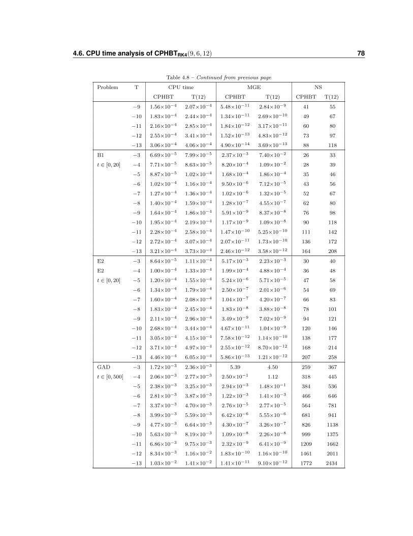
4.6. CPU time analysis of CPHBTRK4(9, 6, 12) 78
Table 4.8 – Continued from previous page
Problem T CPU time MGE NS
CPHBT T(12) CPHBT T(12) CPHBT T(12)
−9 1.56×10⁻⁴ 2.07×10⁻⁴ 5.48×10⁻¹¹ 2.84×10⁻⁹ 41 55
−10 1.83×10⁻⁴ 2.44×10⁻⁴ 1.34×10⁻¹¹ 2.69×10⁻¹⁰ 49 67
−11 2.16×10⁻⁴ 2.85×10⁻⁴ 1.84×10⁻¹² 3.17×10⁻¹¹ 60 80
−12 2.55×10⁻⁴ 3.41×10⁻⁴ 1.52×10⁻¹³ 4.83×10⁻¹² 73 97
−13 3.06×10⁻⁴ 4.06×10⁻⁴ 4.90×10⁻¹⁴ 3.69×10⁻¹³ 88 118
B1 −3 6.69×10⁻⁵ 7.99×10⁻⁵ 2.37×10⁻³ 7.40×10⁻² 26 33
t ∈ [0, 20] −4 7.71×10⁻⁵ 8.63×10⁻⁵ 8.20×10⁻⁴ 1.09×10⁻² 28 39
−5 8.87×10⁻⁵ 1.02×10⁻⁴ 1.68×10⁻⁴ 1.86×10⁻⁴ 35 46
−6 1.02×10⁻⁴ 1.16×10⁻⁴ 9.50×10⁻⁶ 7.12×10⁻⁵ 43 56
−7 1.27×10⁻⁴ 1.36×10⁻⁴ 1.02×10⁻⁶ 1.32×10⁻⁵ 52 67
−8 1.40×10⁻⁴ 1.59×10⁻⁴ 1.28×10⁻⁷ 4.55×10⁻⁷ 62 80
−9 1.64×10⁻⁴ 1.86×10⁻⁴ 5.91×10⁻⁹ 8.37×10⁻⁸ 76 98
−10 1.95×10⁻⁴ 2.19×10⁻⁴ 1.17×10⁻⁹ 1.09×10⁻⁸ 90 118
−11 2.28×10⁻⁴ 2.58×10⁻⁴ 1.47×10⁻¹⁰ 5.25×10⁻¹⁰ 111 142
−12 2.72×10⁻⁴ 3.07×10⁻⁴ 2.07×10⁻¹¹ 1.73×10⁻¹⁰ 136 172
−13 3.21×10⁻⁴ 3.73×10⁻⁴ 2.46×10⁻¹² 3.58×10⁻¹² 164 208
E2 −3 8.64×10⁻⁵ 1.11×10⁻⁴ 5.17×10⁻³ 2.23×10⁻³ 30 40
E2 −4 1.00×10⁻⁴ 1.33×10⁻⁴ 1.99×10⁻⁴ 4.88×10⁻⁴ 36 48
t ∈ [0, 20] −5 1.20×10⁻⁴ 1.55×10⁻⁴ 5.24×10⁻⁶ 5.71×10⁻⁵ 47 58
−6 1.34×10⁻⁴ 1.79×10⁻⁴ 2.50×10⁻⁷ 2.01×10⁻⁶ 54 69
−7 1.60×10⁻⁴ 2.08×10⁻⁴ 1.04×10⁻⁷ 4.20×10⁻⁷ 66 83
−8 1.83×10⁻⁴ 2.45×10⁻⁴ 1.83×10⁻⁸ 3.88×10⁻⁸ 78 101
−9 2.11×10⁻⁴ 2.96×10⁻⁴ 3.49×10⁻⁹ 7.02×10⁻⁹ 94 121
−10 2.68×10⁻⁴ 3.44×10⁻⁴ 4.67×10⁻¹¹ 1.04×10⁻⁹ 120 146
−11 3.05×10⁻⁴ 4.15×10⁻⁴ 7.58×10⁻¹² 1.14×10⁻¹⁰ 138 177
−12 3.71×10⁻⁴ 4.97×10⁻⁴ 2.55×10⁻¹² 8.70×10⁻¹² 168 214
−13 4.46×10⁻⁴ 6.05×10⁻⁴ 5.86×10⁻¹³ 1.21×10⁻¹² 207 258
GAD −3 1.72×10⁻³ 2.36×10⁻³ 5.39 4.50 259 367
t ∈ [0, 500] −4 2.06×10⁻³ 2.77×10⁻³ 2.50×10⁻¹ 1.12 318 445
−5 2.38×10⁻³ 3.25×10⁻³ 2.94×10⁻³ 1.48×10⁻¹ 384 536
−6 2.81×10⁻³ 3.87×10⁻³ 1.22×10⁻³ 1.41×10⁻³ 466 646
−7 3.37×10⁻³ 4.70×10⁻³ 2.76×10⁻⁵ 2.77×10⁻⁵ 564 781
−8 3.99×10⁻³ 5.59×10⁻³ 6.42×10⁻⁶ 5.55×10⁻⁶ 681 941
−9 4.77×10⁻³ 6.64×10⁻³ 4.30×10⁻⁷ 3.26×10⁻⁷ 826 1138
−10 5.63×10⁻³ 8.19×10⁻³ 1.09×10⁻⁸ 2.26×10⁻⁸ 999 1375
−11 6.86×10⁻³ 9.75×10⁻³ 2.32×10⁻⁹ 6.41×10⁻⁹ 1209 1662
−12 8.34×10⁻³ 1.16×10⁻² 1.83×10⁻¹⁰ 1.16×10⁻¹⁰ 1461 2011
−13 1.03×10⁻² 1.41×10⁻² 1.41×10⁻¹¹ 9.10×10⁻¹² 1772 2434
4.7. The propagation of error in a long-term integration problem for CPHBTRK4(9, 6, 12) 79
4.7 The propagation of error in a long-term inte-
gration problem for CPHBTRK4(9, 6, 12)
4.7.1 Fixed step-size configuration
As shown in the previous sections, the designed CPHBTRK4(9, 6, 12) method perform
favourably over T(12), T(12)L and DP(8,7)13M in terms of accuracy and efficiency.
In particular, the CPU time, the number of steps and of function evaluations required
to achieve the user defined tolerance TOL. In addition, CPHBTRK4 satisfies the con-
tractivity preserving property which is a natural property occurring in dissipative
systems of ODEs [33]. T. Nguyen-Ba et al. showed in [40] that the contractivity
preserving property can reduce the propagation of discretization errors in the nu-
merical method. To investigate this property, we test the propagation of error of
CPHBTRK4(9, 6, 12) method compared to Adams-Bashforth-Moulton, ABM(12,11),
method of order 12 with predictor of order 11 and corrector of order 12 in PECE
mode [48, page 135-140]. We will consider Kepler’s two-body problem with eccen-
tricities ε = 0.3, 0.5, 0.7 over the time period t ∈ [0, 800000π]. In this simulation, we
choose fixed step sizes hCPHBT and hABM such that the methods CPHBTRK4(9, 6, 12)
and ABM(12,11) use approximately an equal CPU time. In Figure (4.7), we plot 300
equidistant points of the energy error over the integration period in a log-log scale
using the MATLAB function loglog. We note that this MATLAB function plots the
data in log-log scale, but it leaves the axis linear with logarithmic ticks, i.e., it plots
logarithmic data on linear axes. Also, we used the MATLAB filter command to
remove some chattering in the collected data.
From Figure (4.7), we notice that the energy error (EE) grows asymptotically
as a power law module αtβ. Then, we fit the collected data to the module αtβ. We
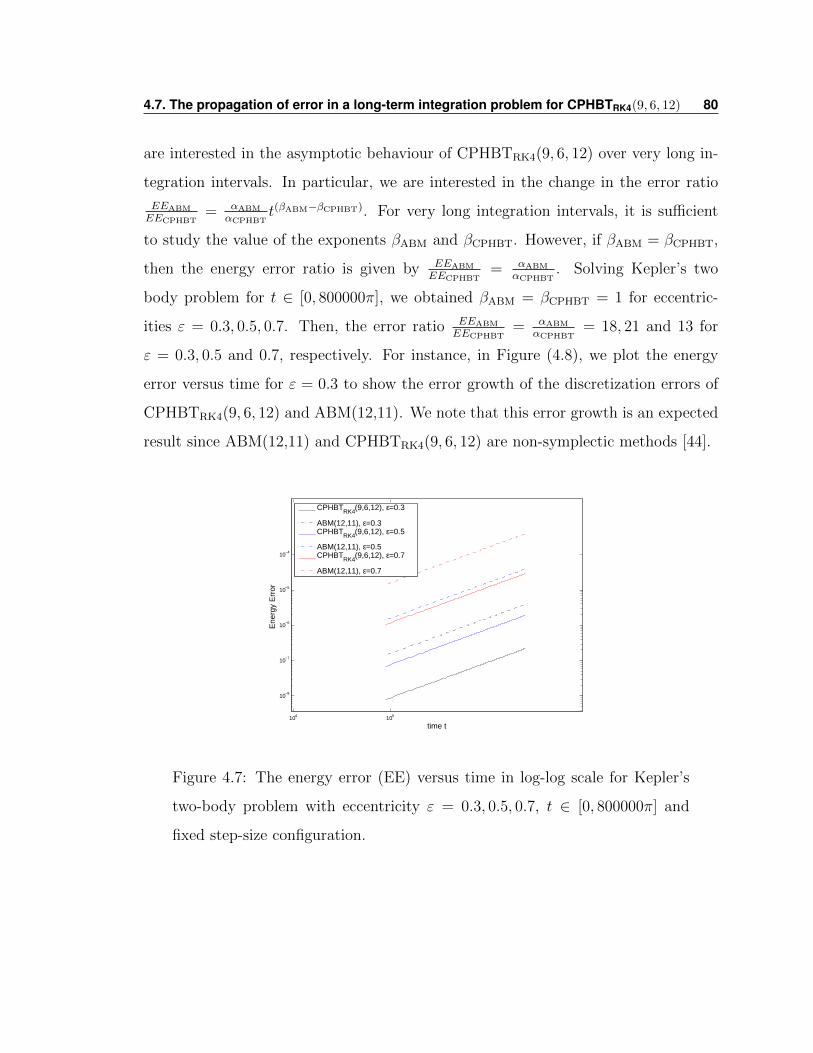
4.7. The propagation of error in a long-term integration problem for CPHBTRK4(9, 6, 12) 80
are interested in the asymptotic behaviour of CPHBTRK4(9, 6, 12) over very long in-
tegration intervals. In particular, we are interested in the change in the error ratio
EEABM
EECPHBT= αABM
αCPHBTt(βABM−βCPHBT). For very long integration intervals, it is sufficient
to study the value of the exponents βABM and βCPHBT. However, if βABM = βCPHBT,
then the energy error ratio is given by EEABM
EECPHBT= αABM
αCPHBT. Solving Kepler’s two
body problem for t ∈ [0, 800000π], we obtained βABM = βCPHBT = 1 for eccentric-
ities ε = 0.3, 0.5, 0.7. Then, the error ratio EEABM
EECPHBT= αABM
αCPHBT= 18, 21 and 13 for
ε = 0.3, 0.5 and 0.7, respectively. For instance, in Figure (4.8), we plot the energy
error versus time for ε = 0.3 to show the error growth of the discretization errors of
CPHBTRK4(9, 6, 12) and ABM(12,11). We note that this error growth is an expected
result since ABM(12,11) and CPHBTRK4(9, 6, 12) are non-symplectic methods [44].
104 105
10−8
10−7
10−6
10−5
10−4
time t
Ene
rgy
Err
or
CPHBTRK4
(9,6,12), ε=0.3
ABM(12,11), ε=0.3CPHBT
RK4(9,6,12), ε=0.5
ABM(12,11), ε=0.5CPHBT
RK4(9,6,12), ε=0.7
ABM(12,11), ε=0.7
Figure 4.7: The energy error (EE) versus time in log-log scale for Kepler’s
two-body problem with eccentricity ε = 0.3, 0.5, 0.7, t ∈ [0, 800000π] and
fixed step-size configuration.
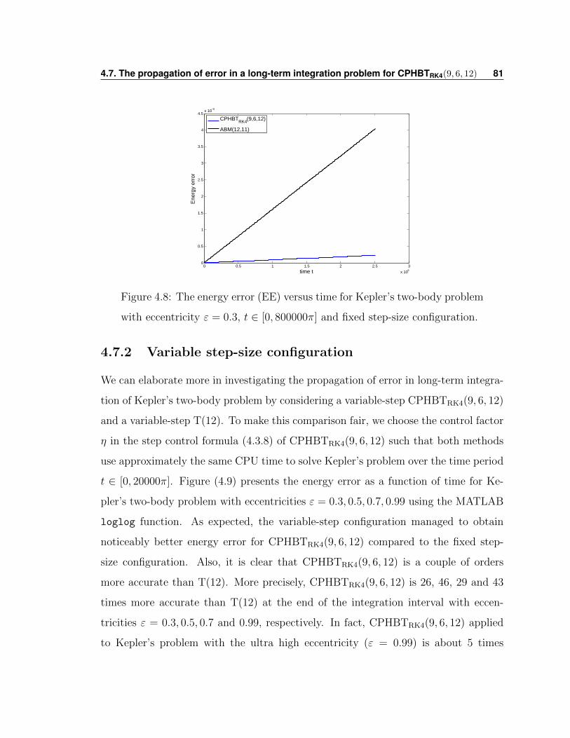
4.7. The propagation of error in a long-term integration problem for CPHBTRK4(9, 6, 12) 81
0 0.5 1 1.5 2 2.5 3
x 106
0
0.5
1
1.5
2
2.5
3
3.5
4
4.5x 10⁻⁶
time t
Ene
rgy
erro
r
CPHBT
RK4(9,6,12)
ABM(12,11)
Figure 4.8: The energy error (EE) versus time for Kepler’s two-body problem
with eccentricity ε = 0.3, t ∈ [0, 800000π] and fixed step-size configuration.
4.7.2 Variable step-size configuration
We can elaborate more in investigating the propagation of error in long-term integra-
tion of Kepler’s two-body problem by considering a variable-step CPHBTRK4(9, 6, 12)
and a variable-step T(12). To make this comparison fair, we choose the control factor
η in the step control formula (4.3.8) of CPHBTRK4(9, 6, 12) such that both methods
use approximately the same CPU time to solve Kepler’s problem over the time period
t ∈ [0, 20000π]. Figure (4.9) presents the energy error as a function of time for Ke-
pler’s two-body problem with eccentricities ε = 0.3, 0.5, 0.7, 0.99 using the MATLAB
loglog function. As expected, the variable-step configuration managed to obtain
noticeably better energy error for CPHBTRK4(9, 6, 12) compared to the fixed step-
size configuration. Also, it is clear that CPHBTRK4(9, 6, 12) is a couple of orders
more accurate than T(12). More precisely, CPHBTRK4(9, 6, 12) is 26, 46, 29 and 43
times more accurate than T(12) at the end of the integration interval with eccen-
tricities ε = 0.3, 0.5, 0.7 and 0.99, respectively. In fact, CPHBTRK4(9, 6, 12) applied
to Kepler’s problem with the ultra high eccentricity (ε = 0.99) is about 5 times
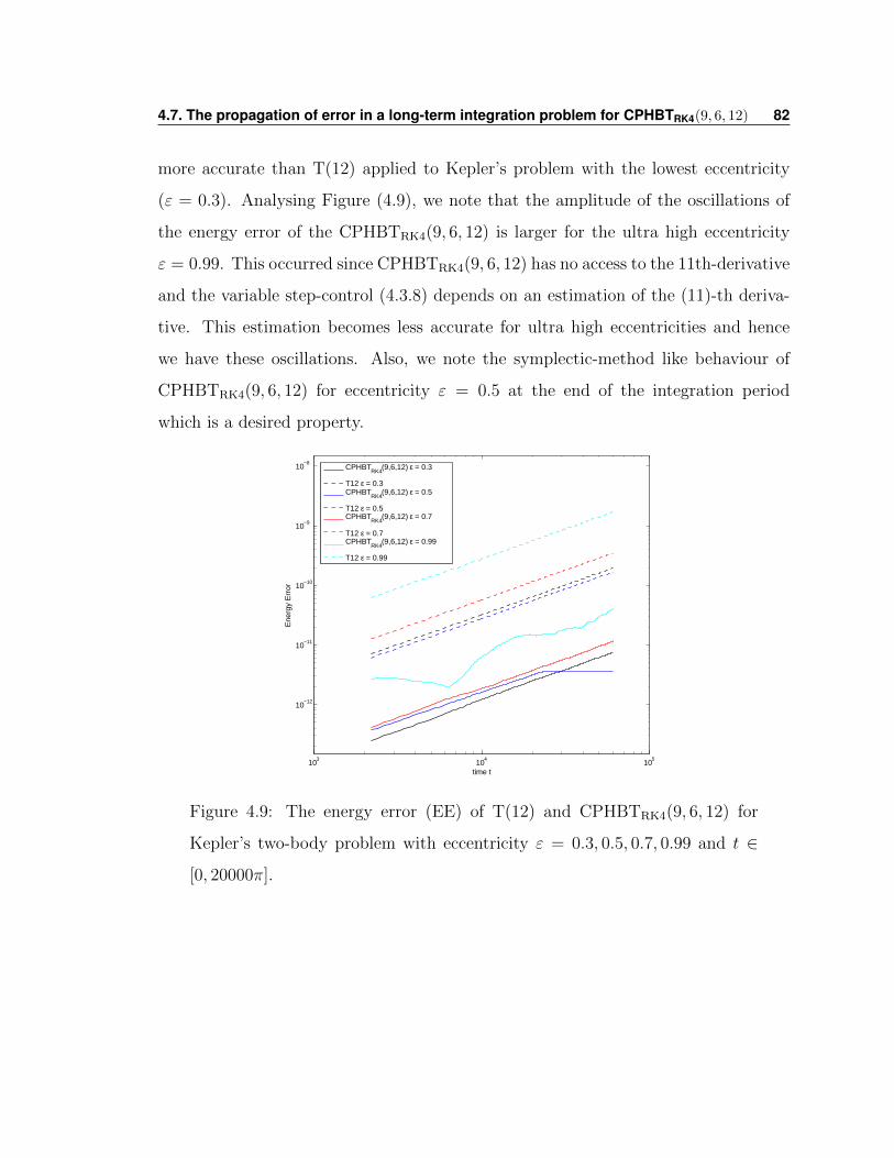
4.7. The propagation of error in a long-term integration problem for CPHBTRK4(9, 6, 12) 82
more accurate than T(12) applied to Kepler’s problem with the lowest eccentricity
(ε = 0.3). Analysing Figure (4.9), we note that the amplitude of the oscillations of
the energy error of the CPHBTRK4(9, 6, 12) is larger for the ultra high eccentricity
ε = 0.99. This occurred since CPHBTRK4(9, 6, 12) has no access to the 11th-derivative
and the variable step-control (4.3.8) depends on an estimation of the (11)-th deriva-
tive. This estimation becomes less accurate for ultra high eccentricities and hence
we have these oscillations. Also, we note the symplectic-method like behaviour of
CPHBTRK4(9, 6, 12) for eccentricity ε = 0.5 at the end of the integration period
which is a desired property.
103
104
105
10−12
10−11
10−10
10−9
10−8
time t
Ene
rgy
Err
or
CPHBTRK4
(9,6,12) ε = 0.3
T12 ε = 0.3CPHBT
RK4(9,6,12) ε = 0.5
T12 ε = 0.5CPHBT
RK4(9,6,12) ε = 0.7
T12 ε = 0.7CPHBT
RK4(9,6,12) ε = 0.99
T12 ε = 0.99
Figure 4.9: The energy error (EE) of T(12) and CPHBTRK4(9, 6, 12) for
Kepler’s two-body problem with eccentricity ε = 0.3, 0.5, 0.7, 0.99 and t ∈
[0, 20000π].
Chapter 5
CP s-Stage HBT methods based
on combining T(d) and RK(s,5)
methods
5.1 Introduction
In the previous chapters, we show that CPHBTRK4(d, s, p) performs favourably in
comparison with many well known methods such as T(12), T(12)L, DP(8,7)M13 and
Adams-Bashforth-Moulton methods in terms of the NS, NFE and CPU time PEG
required to satisfy a given user defined tolerance TOL. Also, we show the effect of
the contractivity preserving property of CPHBTRK4 by considering the long term
integration of Kepler’s two-body problem where CPHBTRK4(d, s, p) was superior to
the other considered well known methods. These results motivated us to investi-
gate and design the second set of CPHBT methods by casting Runge-Kutta meth-
ods of order 5, RK(s,5), with Taylor method of order p − 4, T(p − 4), and obtain
CPHBTRK5(p − 4, s, p). By considering RK(s,5) instead of RK(s,4), we managed to
reduce the number of computationally expensive high order derivatives (HOD) re-
83
5.2. Formulation of CPHBTRK5(p− 4, s, p) in Butcher form 84
quired to reach order p from p − 2 and p − 3 HOD for CPHBTRK4 to p − 4 for the
CPHBTRK5. Moreover, CPHBTRK5(p− 4, s, p) tends to have larger optimal contrac-
tivity preserving coefficients and larger stability regions.
5.2 Formulation of CPHBTRK5(p−4, s, p) in Butcher
form
To obtain the explicit, one-step, s-stage, (p− 4)-derivative CPHBT method of order
p, Hermite-Birkhoff interpolation polynomials are used to define the following s for-
mulae which performs the integration from xn to xn+1. HB polynomials are used as
predictors Pi to obtain the stages Yi to order p− 4 as follows:
Yi = yn + ∆xi−1∑j=1
ai,jFj +
p−4∑m=2
(∆x)mγi,m y(m)n , i = 2, 3, . . . , s. (5.2.1)
Also, a Hermite-Birkhoff interpolation polynomial is used as an integration formula
(IF) to obtain yn+1 to order p as follows:
yn+1 = yn + ∆xs∑j=1
bjFj +
p−4∑m=2
(∆x)mγs+1,m y(m)n , (5.2.2)
Since CPHBTRK5(p−4, s, p) has a similar form as CPHBTRK4(d, s, p) with d = p−4,
then all contractivity preserving formulations, theorems and the different forms of
CPHBTRK4(d, s, p) can be easily extended to the CPHBTRK5(p − 4, s, p) and hence
these derivations will be omitted in this chapter.
5.3 The order conditions of CPHBTRK5(p− 4, s, p)
To derive the order conditions of CPHBTRK5(p − 4, s, p) obtained by combining
RK(s,5) of order 5 and Taylor method of order p−4, T(p−4), we follow a similar ap-
proach as in Section 3.3. We note that the new set of methods, CPHBTRK5(p−4, s, p),
5.3. The order conditions of CPHBTRK5(p− 4, s, p) 85
have similar formula as the first set of methods, CPHBTRK4(d, s, p), with d = p− 4.
Then, the elementary weights of CPHBTRK5(p − 4, s, p) are given by the recursive
formulas (3.3.17)-(3.3.21) with d = p−4 and hence we can derive the order conditions
of CPHBTRK5(p − 4, s, p) by enforcing equation (3.3.16). As an example, we derive
the order condition of CPHBTRK5(2, s, 6) of order 6 associated with the rooted tree
t34 = [τ 2[τ 2]2. By equations (3.3.17)-(3.3.21), the elementary weight Ψ(t34) is given
by
Ψ(t34) =s∑j=1
bjS′j(t34) +
2∑m=2
γimΦ(m)(t34)
=s∑j=1
bjS′j(t34) = 6
s∑j=1
bj(Sj(τ)
)2Sj([τ
2]), (5.3.1)
with,
Sj(τ) =
j−1∑k=1
ajkS′k(τ) =
j−1∑k=1
ajk = cj, (5.3.2)
S ′j([τ2]) =
j−1∑l=1
ajlS′l([τ
2]) = 3
j−1∑l=1
ajl(Sl(τ)
)2= 3
j−1∑l=1
ajlc2l . (5.3.3)
Substituting equations (5.3.2) and (5.3.3) into (5.3.1), the elementary weight of
CPHBTRK5(2, s, 6) corresponding to the rooted tree t34 = [τ 2[τ 2]2 is
Ψ(t34) = 18s∑j=1
bjc2j
[ j−1∑l=1
ajlc2l
]. (5.3.4)
Hence, by equation (3.3.16), the order condition of CPHBTRK5(2, s, 6) corresponding
to the rooted tree t34 is given by
Ψ(t34) = 1⇐⇒s∑j=1
bjc2j
[ j−1∑l=1
ajlc2l
]=
1
18, (5.3.5)
which is the order condition (5.3.20) given below for p = 6.
5.3. The order conditions of CPHBTRK5(p− 4, s, p) 86
To reduce the number of independent order conditions, we impose the following
simplifying conditions [22, 41]:
i−1∑j=1
ai,jckjk!
+ γi,k+1 =1
(k + 1)!ck+1i ,
i = 2, 3, . . . , s,
k = 0, 1, . . . , p− 5.
(5.3.6)
Again, we take c1 = 0, the convention that c01 = 1 and γi,1 = 0 for i = 2, 3, . . . , s. By
enforcing these simplifying conditions, all order conditions of CPHBTRK5(p− 4, s, p)
generated from trees of order r = 1, 2, . . . , p − 3 are equivalent to those generated
by the bushy trees of order r = 1, 2, . . . , p− 3 and the number of independent order
conditions generated from trees of orders r = p − 2, p − 1, p is reduced considerably.
For instance, when we derive the order conditions of CPHBTRK5(8, s, 12) of order 12,
the simplifying conditions (5.3.6) reduces the number of order conditions from 7813
independent conditions to only 95 independent conditions including the simplifying
conditions. We note that, when deriving CPHBTRK4(d, s, 12) by casting T(d) with
RK(s,4) of order 4 in the previous chapter, the simplifying conditions (3.3.29) reduced
the number of order conditions from 7813 independent conditions to 52 only. The
remaining trees will lead to the following sets of order conditions for CPHBTRK5(p−
4, s, p) :
s∑i=1
bi = 1, (5.3.7)
s∑i=2
bicki + k!γs+1,k+1 =
1
k + 1, k = 1, . . . , p− 5, (5.3.8)
s∑i=2
bicki =
1
k + 1, k = p− 4, p− 3, p− 2, p− 1, (5.3.9)
s∑i=3
bi
[ i−1∑j=2
ai,j cp−4j
]=
1
(p− 2)(p− 3), (5.3.10)
s∑i=4
bi
[ i−1∑j=3
ai,j
[ j−1∑k=2
aj,k cp−4k
]]=
1
(p− 1)(p− 2)(p− 3), (5.3.11)
5.4. Formulation of the optimization problem of CPHBTRK5(p− 4, s, p) 87
s∑i=3
bi
[ i−1∑j=2
ai,j cp−3j
]=
1
(p− 1)(p− 2), (5.3.12)
s∑i=3
bici
[ i−1∑j=2
ai,j cp−4j
]=
1
(p− 1)(p− 3), (5.3.13)
s∑i=5
bi
[ i−1∑j=4
ai,j
[ j−1∑k=3
aj,k
(k−1∑l=2
ak,l cp−4l
)]]=
1
p(p− 1)(p− 2)(p− 3), (5.3.14)
s∑i=4
bi
[ i−1∑j=3
ai,j
[ j−1∑k=2
aj,k cp−3k
]]=
1
p(p− 1)(p− 2), (5.3.15)
s∑i=4
bi
[ i−1∑j=3
ai,jcj
[ j−1∑k=2
aj,k cp−4k
]]=
1
p(p− 1)(p− 3), (5.3.16)
s∑i=3
bi
[ i−1∑j=2
ai,j cp−2j
]=
1
p(p− 1), (5.3.17)
s∑i=4
bici
[ i−1∑j=3
ai,j
[ j−1∑k=2
aj,k cp−4k
]]=
1
p(p− 2)(p− 3), (5.3.18)
s∑i=3
bici
[ i−1∑j=2
ai,j cp−3j
]=
1
p(p− 2), (5.3.19)
s∑i=3
bic2i
[ i−1∑j=2
ai,j cp−4j
]=
1
p(p− 3). (5.3.20)
5.4 Formulation of the optimization problem of
CPHBTRK5(p− 4, s, p)
Considering the conditions of the contractivity preserving property in Theorem (3.7.1)
together with the simplifying conditions (5.3.6) and the order conditions (5.3.7)-
(5.3.20), we can obtain a feasible CPHBTRK5(p− 4, s, p) with a feasible contractivity
preserving coefficient cfcp as mentioned in Remark 3.4.1. However, following our work
in Section 3.8, we obtain an optimal CPHBTRK5(p−4, s, p) with largest contractivity
5.5. Construction of optimal CPHBTRK5(p− 4, s, p) 88
preserving coefficient by solving the following nonlinear optimization problem:
maximizez,v,α,β,δ
F (z,v,α,β, δ) = z (5.4.1)
subject to
αij − zβij = 0,
i = 3, 4, . . . , s+ 1,
j = 2, 3, . . . , i− 1,
(5.4.2)
(I + zβ0)−1 v0 ≥ 0, (5.4.3)
(I + zβ0)−1 β0 ≥ 0, (5.4.4)
(I + zβ0)−1 γ0 ≥ 0, (5.4.5)
0 ≤ ci ≤ 1 i = 2, 3, . . . , s+ 1, (5.4.6)
z ≤ zi1 =αi1βi1
i = 2, 3, . . . , s+ 1, (5.4.7)
δi,mzmi1m!− αi,1 ≤ 0,
i = 2, 3, . . . , s+ 1,
m = 2, 3, . . . , p− 4
(5.4.8)
together with
• The simplifying conditions (5.3.6),
• The set of order conditions (5.3.7)-(5.3.20),
where the objective function is defined in (3.8.8), the inequalities (5.4.3)-(5.4.5) are
taken component-wise and the coefficient matrices v0,β0,γ0 and δ are defined in
equations (3.6.5), (3.4.4) and (3.5.3).
5.5 Construction of optimal CPHBTRK5(p− 4, s, p)
Indeed, the number of constraints in the above mentioned optimization problem
is considerably larger than the optimization problem of CPHBTRK4. Our numeri-
cal search for 6-stages methods failed to satisfy some of the constraints, especially
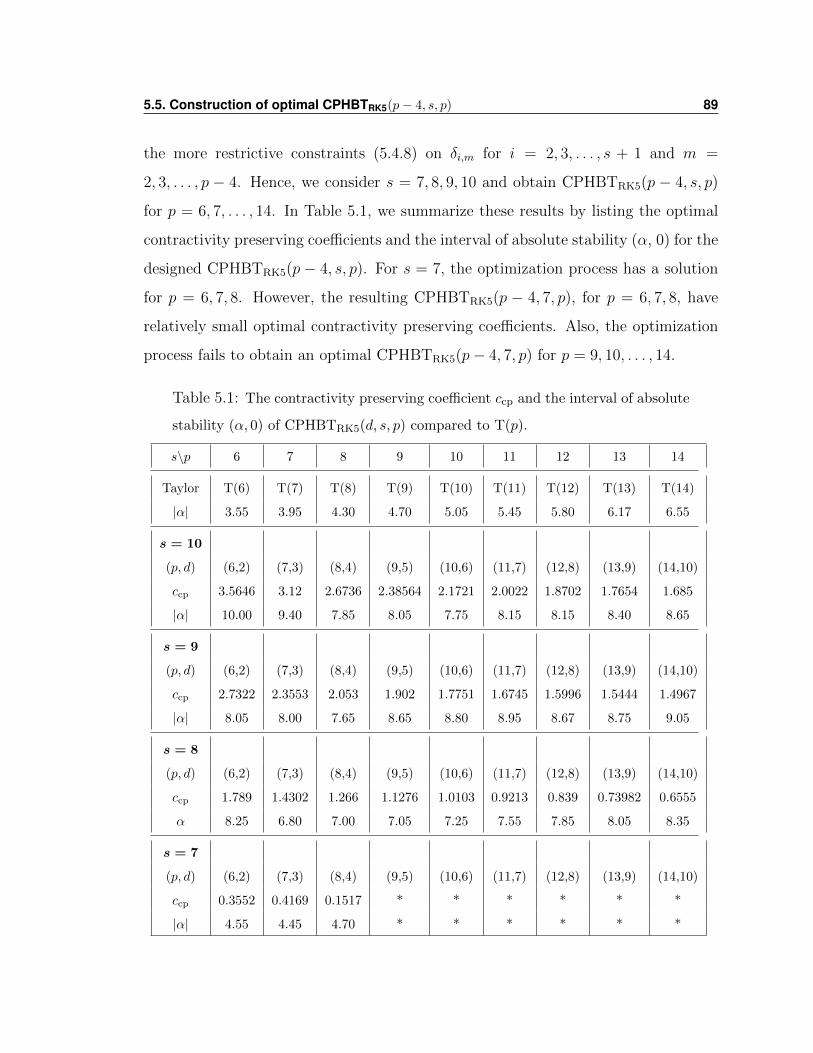
5.5. Construction of optimal CPHBTRK5(p− 4, s, p) 89
the more restrictive constraints (5.4.8) on δi,m for i = 2, 3, . . . , s + 1 and m =
2, 3, . . . , p − 4. Hence, we consider s = 7, 8, 9, 10 and obtain CPHBTRK5(p − 4, s, p)
for p = 6, 7, . . . , 14. In Table 5.1, we summarize these results by listing the optimal
contractivity preserving coefficients and the interval of absolute stability (α, 0) for the
designed CPHBTRK5(p − 4, s, p). For s = 7, the optimization process has a solution
for p = 6, 7, 8. However, the resulting CPHBTRK5(p − 4, 7, p), for p = 6, 7, 8, have
relatively small optimal contractivity preserving coefficients. Also, the optimization
process fails to obtain an optimal CPHBTRK5(p− 4, 7, p) for p = 9, 10, . . . , 14.
Table 5.1: The contractivity preserving coefficient ccp and the interval of absolute
stability (α, 0) of CPHBTRK5(d, s, p) compared to T(p).
s\p 6 7 8 9 10 11 12 13 14
Taylor T(6) T(7) T(8) T(9) T(10) T(11) T(12) T(13) T(14)
|α| 3.55 3.95 4.30 4.70 5.05 5.45 5.80 6.17 6.55
s = 10
(p, d) (6,2) (7,3) (8,4) (9,5) (10,6) (11,7) (12,8) (13,9) (14,10)
ccp 3.5646 3.12 2.6736 2.38564 2.1721 2.0022 1.8702 1.7654 1.685
|α| 10.00 9.40 7.85 8.05 7.75 8.15 8.15 8.40 8.65
s = 9
(p, d) (6,2) (7,3) (8,4) (9,5) (10,6) (11,7) (12,8) (13,9) (14,10)
ccp 2.7322 2.3553 2.053 1.902 1.7751 1.6745 1.5996 1.5444 1.4967
|α| 8.05 8.00 7.65 8.65 8.80 8.95 8.67 8.75 9.05
s = 8
(p, d) (6,2) (7,3) (8,4) (9,5) (10,6) (11,7) (12,8) (13,9) (14,10)
ccp 1.789 1.4302 1.266 1.1276 1.0103 0.9213 0.839 0.73982 0.6555
α 8.25 6.80 7.00 7.05 7.25 7.55 7.85 8.05 8.35
s = 7
(p, d) (6,2) (7,3) (8,4) (9,5) (10,6) (11,7) (12,8) (13,9) (14,10)
ccp 0.3552 0.4169 0.1517 * * * * * *
|α| 4.55 4.45 4.70 * * * * * *
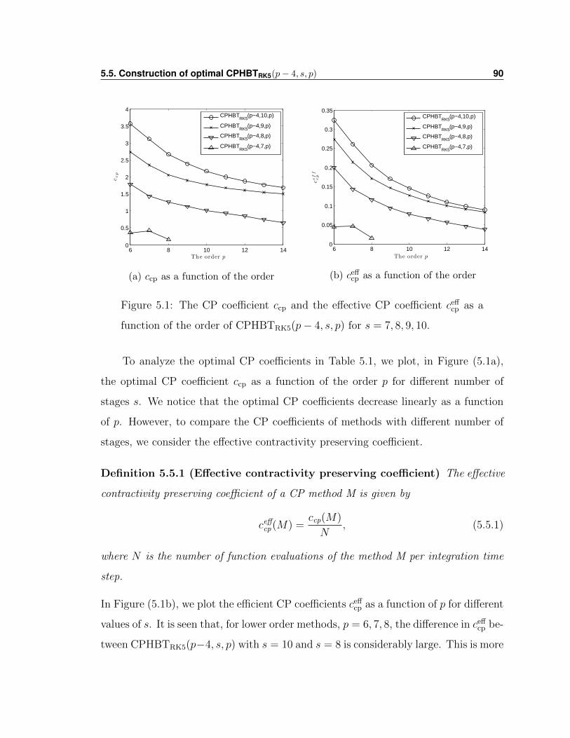
5.5. Construction of optimal CPHBTRK5(p− 4, s, p) 90
6 8 10 12 140
0.5
1
1.5
2
2.5
3
3.5
4
The order p
ccp
CPHBT
RK5(p−4,10,p)
CPHBTRK5
(p−4,9,p)
CPHBTRK5
(p−4,8,p)
CPHBTRK5
(p−4,7,p)
(a) ccp as a function of the order
6 8 10 12 140
0.05
0.1
0.15
0.2
0.25
0.3
0.35
The order p
ceff
cp
CPHBT
RK5(p−4,10,p)
CPHBTRK5
(p−4,9,p)
CPHBTRK5
(p−4,8,p)
CPHBTRK5
(p−4,7,p)
(b) ceffcp as a function of the order
Figure 5.1: The CP coefficient ccp and the effective CP coefficient ceffcp as a
function of the order of CPHBTRK5(p− 4, s, p) for s = 7, 8, 9, 10.
To analyze the optimal CP coefficients in Table 5.1, we plot, in Figure (5.1a),
the optimal CP coefficient ccp as a function of the order p for different number of
stages s. We notice that the optimal CP coefficients decrease linearly as a function
of p. However, to compare the CP coefficients of methods with different number of
stages, we consider the effective contractivity preserving coefficient.
Definition 5.5.1 (Effective contractivity preserving coefficient) The effective
contractivity preserving coefficient of a CP method M is given by
ceffcp (M) =
ccp(M)
N, (5.5.1)
where N is the number of function evaluations of the method M per integration time
step.
In Figure (5.1b), we plot the efficient CP coefficients ceffcp as a function of p for different
values of s. It is seen that, for lower order methods, p = 6, 7, 8, the difference in ceffcp be-
tween CPHBTRK5(p−4, s, p) with s = 10 and s = 8 is considerably large. This is more
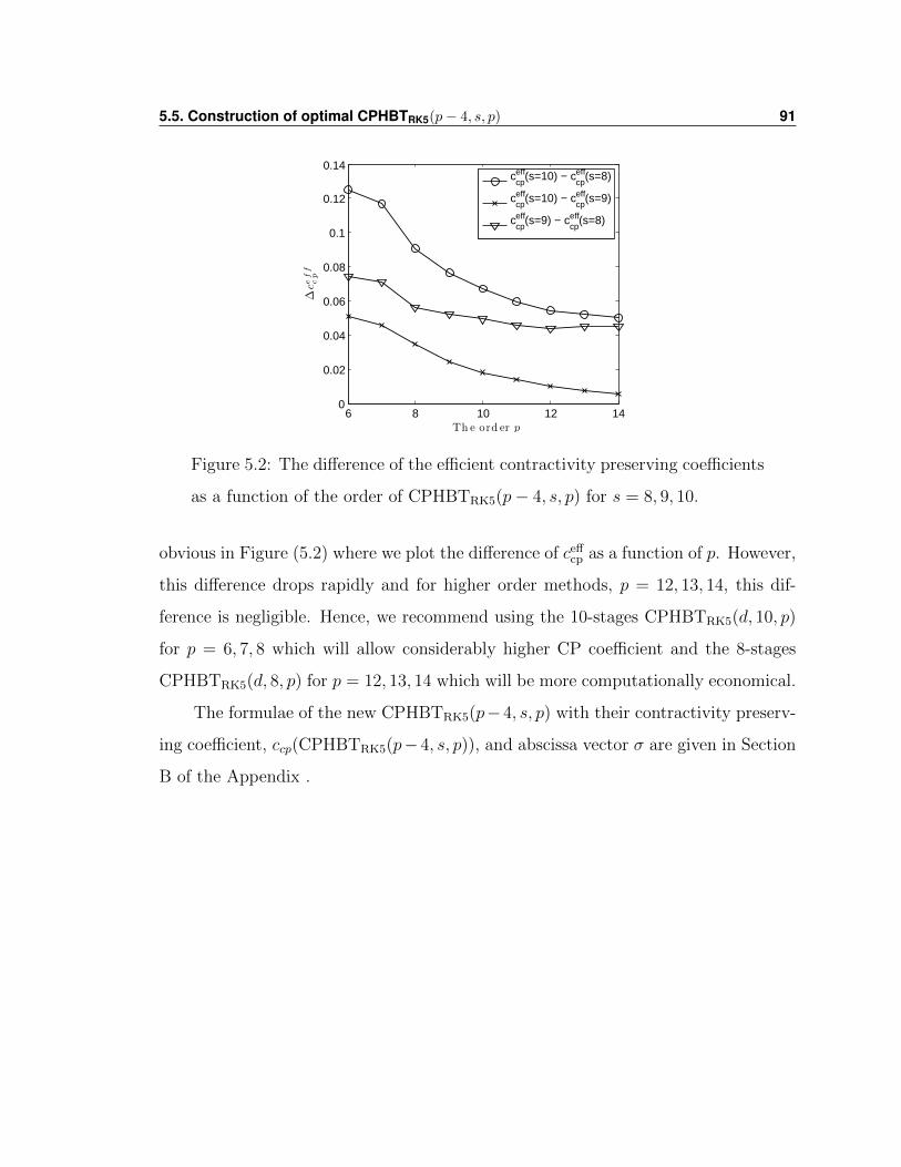
5.5. Construction of optimal CPHBTRK5(p− 4, s, p) 91
6 8 10 12 140
0.02
0.04
0.06
0.08
0.1
0.12
0.14
Th e ord er p
∆ce
ff
cp
c
cpeff(s=10) − c
cpeff(s=8)
ccpeff(s=10) − c
cpeff(s=9)
ccpeff(s=9) − c
cpeff(s=8)
Figure 5.2: The difference of the efficient contractivity preserving coefficients
as a function of the order of CPHBTRK5(p− 4, s, p) for s = 8, 9, 10.
obvious in Figure (5.2) where we plot the difference of ceffcp as a function of p. However,
this difference drops rapidly and for higher order methods, p = 12, 13, 14, this dif-
ference is negligible. Hence, we recommend using the 10-stages CPHBTRK5(d, 10, p)
for p = 6, 7, 8 which will allow considerably higher CP coefficient and the 8-stages
CPHBTRK5(d, 8, p) for p = 12, 13, 14 which will be more computationally economical.
The formulae of the new CPHBTRK5(p−4, s, p) with their contractivity preserv-
ing coefficient, ccp(CPHBTRK5(p− 4, s, p)), and abscissa vector σ are given in Section
B of the Appendix .
Chapter 6
Numerical results for the designed
CPHBTRK5(p− 4, s, p) methods
obtained from T(p− 4) and RK(s,5)
methods
In this chapter, we present some numerical results obtained by testing the second set of
CPHBTRK5 in terms of maximum global error (MGE), maximum global energy error
(MGEE), number of steps (NS), number of function evaluations (NFE), CPU time
and the propagation of errors in long-term integration problems. For consistency and
comparison reasons, we will consider an 8-stage, 8-derivatives CPHBTRK5(8, 8, 12) of
order 12 as a representative of the designed CPHBTRK5 methods.
92
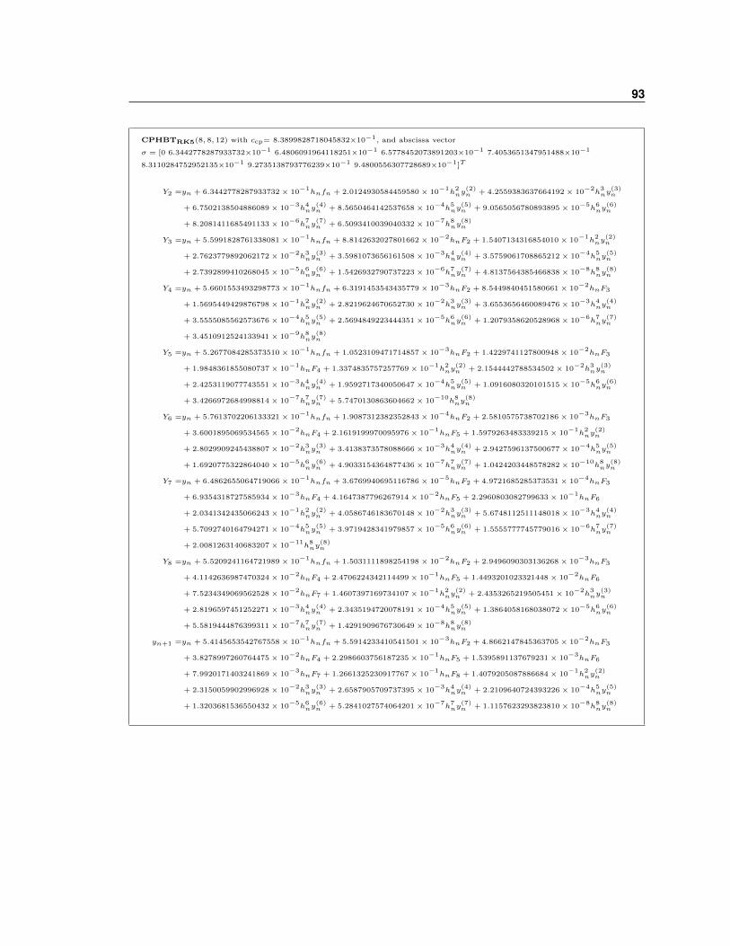
93
CPHBTRK5(8, 8, 12) with ccp= 8.3899828718045832×10⁻¹, and abscissa vector
σ = [0 6.3442778287933732×10⁻¹ 6.4806091964118251×10⁻¹ 6.5778452073891203×10⁻¹ 7.4053651347951488×10⁻¹
8.3110284752952135×10⁻¹ 9.2735138793776239×10⁻¹ 9.4800556307728689×10⁻¹]T
Y2 =yn + 6.3442778287933732 × 10⁻¹hnfn + 2.0124930584459580 × 10
−1h2ny
(2)n + 4.2559383637664192 × 10
−2h3ny
(3)n
+ 6.7502138504886089 × 10⁻³h4ny
(4)n + 8.5650464142537658 × 10
−4h5ny
(5)n + 9.0565056780893895 × 10
−5h6ny
(6)n
+ 8.2081411685491133 × 10⁻⁶h7ny
(7)n + 6.5093410039040332 × 10
−7h8ny
(8)n
Y3 =yn + 5.5991828761338081 × 10⁻¹hnfn + 8.8142632027801662 × 10
−2hnF2 + 1.5407134316854010 × 10
−1h2ny
(2)n
+ 2.7623779892062172 × 10⁻²h3ny
(3)n + 3.5981073656161508 × 10
−3h4ny
(4)n + 3.5759061708865212 × 10
−4h5ny
(5)n
+ 2.7392899410268045 × 10⁻⁵h6ny
(6)n + 1.5426932790737223 × 10
−6h7ny
(7)n + 4.8137564385466838 × 10
−8h8ny
(8)n
Y4 =yn + 5.6601553493298773 × 10⁻¹hnfn + 6.3191453543435779 × 10
−3hnF2 + 8.5449840451580661 × 10
−2hnF3
+ 1.5695449429876798 × 10⁻¹h2ny
(2)n + 2.8219624670652730 × 10
−2h3ny
(3)n + 3.6553656460089476 × 10
−3h4ny
(4)n
+ 3.5555085562573676 × 10⁻⁴h5ny
(5)n + 2.5694849223444351 × 10
−5h6ny
(6)n + 1.2079358620528968 × 10
−6h7ny
(7)n
+ 3.4510912524133941 × 10⁻⁹h8ny
(8)n
Y5 =yn + 5.2677084285373510 × 10⁻¹hnfn + 1.0523109471714857 × 10
−3hnF2 + 1.4229741127800948 × 10
−2hnF3
+ 1.9848361855080737 × 10⁻¹hnF4 + 1.3374835757257769 × 10
−1h2ny
(2)n + 2.1544442788534502 × 10
−2h3ny
(3)n
+ 2.4253119077743551 × 10⁻³h4ny
(4)n + 1.9592717340050647 × 10
−4h5ny
(5)n + 1.0916080320101515 × 10
−5h6ny
(6)n
+ 3.4266972684998814 × 10⁻⁷h7ny
(7)n + 5.7470130863604662 × 10
−10h8ny
(8)n
Y6 =yn + 5.7613702206133321 × 10⁻¹hnfn + 1.9087312382352843 × 10
−4hnF2 + 2.5810575738702186 × 10
−3hnF3
+ 3.6001895069534565 × 10⁻²hnF4 + 2.1619199970095976 × 10
−1hnF5 + 1.5979263483339215 × 10
−1h2ny
(2)n
+ 2.8029909245438807 × 10⁻²h3ny
(3)n + 3.4138373578088666 × 10
−3h4ny
(4)n + 2.9427596137500677 × 10
−4h5ny
(5)n
+ 1.6920775322864040 × 10⁻⁵h6ny
(6)n + 4.9033154364877436 × 10
−7h7ny
(7)n + 1.0424203448578282 × 10
−10h8ny
(8)n
Y7 =yn + 6.4862655064719066 × 10⁻¹hnfn + 3.6769940695116786 × 10
−5hnF2 + 4.9721685285373531 × 10
−4hnF3
+ 6.9354318727585934 × 10⁻³hnF4 + 4.1647387796267914 × 10
−2hnF5 + 2.2960803082799633 × 10
−1hnF6
+ 2.0341342435066243 × 10⁻¹h2ny
(2)n + 4.0586746183670148 × 10
−2h3ny
(3)n + 5.6748112511148018 × 10
−3h4ny
(4)n
+ 5.7092740164794271 × 10⁻⁴h5ny
(5)n + 3.9719428341979857 × 10
−5h6ny
(6)n + 1.5555777745779016 × 10
−6h7ny
(7)n
+ 2.0081263140683207 × 10⁻¹¹
h8ny
(8)n
Y8 =yn + 5.5209241164721989 × 10⁻¹hnfn + 1.5031111898254198 × 10
−2hnF2 + 2.9496090303136268 × 10
−3hnF3
+ 4.1142636987470324 × 10⁻²hnF4 + 2.4706224342114499 × 10
−1hnF5 + 1.4493201023321448 × 10
−2hnF6
+ 7.5234349069562528 × 10⁻²hnF7 + 1.4607397169734107 × 10
−1h2ny
(2)n + 2.4353265219505451 × 10
−2h3ny
(3)n
+ 2.8196597451252271 × 10⁻³h4ny
(4)n + 2.3435194720078191 × 10
−4h5ny
(5)n + 1.3864058168038072 × 10
−5h6ny
(6)n
+ 5.5819444876399311 × 10⁻⁷h7ny
(7)n + 1.4291909676730649 × 10
−8h8ny
(8)n
yn+1 =yn + 5.4145653542767558 × 10⁻¹hnfn + 5.5914233410541501 × 10
−3hnF2 + 4.8662147845363705 × 10
−2hnF3
+ 3.8278997260764475 × 10⁻²hnF4 + 2.2986603756187235 × 10
−1hnF5 + 1.5395891137679231 × 10
−3hnF6
+ 7.9920171403241869 × 10⁻³hnF7 + 1.2661325230917767 × 10
−1hnF8 + 1.4079205087886684 × 10
−1h2ny
(2)n
+ 2.3150059902996928 × 10⁻²h3ny
(3)n + 2.6587905709737395 × 10
−3h4ny
(4)n + 2.2109640724393226 × 10
−4h5ny
(5)n
+ 1.3203681536550432 × 10⁻⁵h6ny
(6)n + 5.2841027574064201 × 10
−7h7ny
(7)n + 1.1157623293823810 × 10
−8h8ny
(8)n
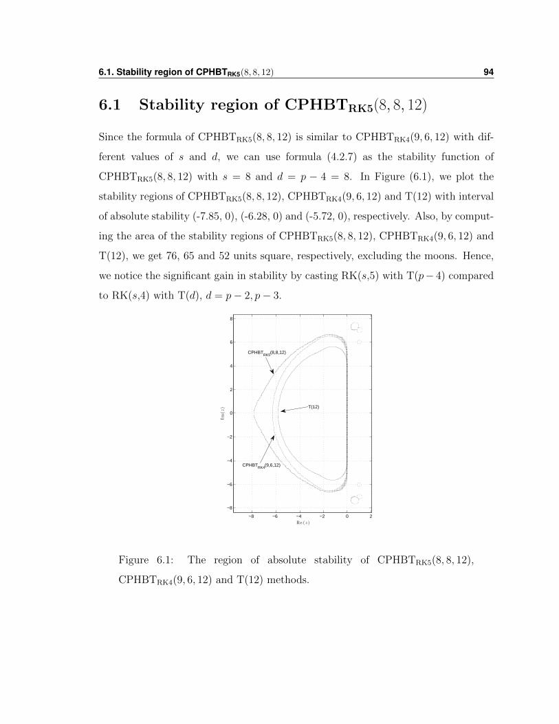
6.1. Stability region of CPHBTRK5(8, 8, 12) 94
6.1 Stability region of CPHBTRK5(8, 8, 12)
Since the formula of CPHBTRK5(8, 8, 12) is similar to CPHBTRK4(9, 6, 12) with dif-
ferent values of s and d, we can use formula (4.2.7) as the stability function of
CPHBTRK5(8, 8, 12) with s = 8 and d = p − 4 = 8. In Figure (6.1), we plot the
stability regions of CPHBTRK5(8, 8, 12), CPHBTRK4(9, 6, 12) and T(12) with interval
of absolute stability (-7.85, 0), (-6.28, 0) and (-5.72, 0), respectively. Also, by comput-
ing the area of the stability regions of CPHBTRK5(8, 8, 12), CPHBTRK4(9, 6, 12) and
T(12), we get 76, 65 and 52 units square, respectively, excluding the moons. Hence,
we notice the significant gain in stability by casting RK(s,5) with T(p− 4) compared
to RK(s,4) with T(d), d = p− 2, p− 3.
−8 −6 −4 −2 0 2
−8
−6
−4
−2
0
2
4
6
8
Re (z)
Im(z
)
CPHBTRK5
(8,8,12)
CPHBTRK4
(9,6,12)
T(12)
Figure 6.1: The region of absolute stability of CPHBTRK5(8, 8, 12),
CPHBTRK4(9, 6, 12) and T(12) methods.
6.2. NS and NFE analysis of CPHBTRK5(8, 8, 12) 95
6.2 NS and NFE analysis of CPHBTRK5(8, 8, 12)
For consistency and comparison, we will consider the same test problems as in the
numerical results of CPHBTRK4 to test the second set of methods CPHBTRK5. The
problems are composed of two sets. The first set consists of Hamiltonian problems
such as the 5 D-class DETEST problems, Kepler’s two-body problem with ultra high
eccentricity ε = 0.99, the HH and EqMP test problems. The second set of problems
consists of the B-class, E-class DETEST problems together with Arenstorf and the
Galactic dynamics problems. The user defined tolerance, TOL, is the desired accuracy
for a certain problem. Some numerical integration problems may run for hundreds of
hours or even a few years in some astronomical simulations. Then, we are interested
in reaching a desired or acceptable accuracy, the user defined tolerance, using minimal
number of integration steps (NS), function evaluations (NFE) and CPU time.
In Table 6.1, we test CPHBTRK5(8, 8, 12) method on the set of Hamiltonian prob-
lems compared to T(12) and T(12)L. We show that although CPHBTRK5(8, 8, 12) re-
quires less integration steps compared to T(12) and T(12)L in all the considered test
problems, it achieves remarkably higher accuracy. Also, comparing similar results
for CPHBTRK4(9, 6, 12) in Table 4.2, we notice that CPHBTRK5(8, 8, 12) performs
favourably considering the NS and MGEE simultaneously. These results confirms that
the error estimation and step control formula (4.3.8) with d = 8 and s = 8 is perform-
ing well in estimating the error and optimizing the step size for CPHBTRK5(8, 8, 12)
to achieve the user defined tolerance using minimal NFE and hence minimal CPU
time.
Moreover, since CPHBTRK5(8, 8, 12) is of order 12, we extend the data given
in Table 6.1 to 10−13 ≤TOL≤ 10−4 and we plot the log10(MGEE) as a function of
the number of steps (NS) in Figure (6.2) for CPHBTRK5(8, 8, 12), T(12) and T(12)L.
Indeed, CPHBTRK5(8, 8, 12) clearly performs better than T(12) and T(12)L even for
the Kepler two-body problem with ultra high eccentricity ε = 0.99. To measure
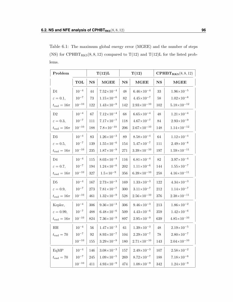
6.2. NS and NFE analysis of CPHBTRK5(8, 8, 12) 96
Table 6.1: The maximum global energy error (MGEE) and the number of steps
(NS) for CPHBTRK5(8, 8, 12) compared to T(12) and T(12)L for the listed prob-
lems.
Problem T(12)L T(12) CPHBTRK5(8, 8, 12)
TOL NS MGEE NS MGEE NS MGEE
D1 10−4 44 7.52×10⁻⁴ 48 6.46×10⁻⁴ 33 1.96×10⁻⁵
ε = 0.1, 10−7 73 1.15×10⁻⁶ 82 4.45×10⁻⁷ 58 1.02×10⁻⁸
tend = 16π 10−10 122 1.43×10⁻⁹ 142 2.93×10⁻¹⁰ 102 5.18×10⁻¹²
D2 10−4 67 7.12×10⁻⁴ 68 6.65×10⁻⁴ 48 1.21×10⁻⁴
ε = 0.3, 10−7 111 7.17×10⁻⁷ 118 4.67×10⁻⁷ 84 2.93×10⁻⁹
tend = 16π 10−10 188 7.8×10⁻¹⁰ 206 2.67×10⁻¹⁰ 148 1.14×10⁻¹²
D3 10−4 83 1.26×10⁻³ 89 8.58×10⁻⁴ 64 1.12×10⁻⁴
ε = 0.5, 10−7 139 1.55×10⁻⁶ 154 5.47×10⁻⁷ 111 2.49×10⁻⁸
tend = 16π 10−10 235 1.87×10⁻⁹ 271 3.39×10⁻¹⁰ 197 1.59×10⁻¹¹
D4 10−4 115 8.03×10⁻⁴ 116 6.81×10⁻⁴ 82 3.97×10⁻⁴
ε = 0.7, 10−7 194 1.24×10⁻⁶ 202 1.11×10⁻⁶ 144 1.55×10⁻⁷
tend = 16π 10−10 327 1.5×10⁻⁹ 356 6.39×10⁻¹⁰ 258 4.16×10⁻¹¹
D5 10−4 167 2.73×10⁻³ 169 1.33×10⁻³ 122 4.34×10⁻³
ε = 0.9, 10−7 273 7.81×10⁻⁷ 300 3.11×10⁻⁷ 212 1.14×10⁻⁷
tend = 16π 10−10 461 1.32×10⁻⁹ 528 2.56×10⁻¹⁰ 376 2.38×10⁻¹¹
Kepler, 10−4 306 9.36×10⁻³ 306 9.46×10⁻³ 213 1.86×10⁻²
ε = 0.99, 10−7 488 6.48×10⁻⁶ 509 4.43×10⁻⁶ 359 1.42×10⁻⁶
tend = 16π 10−10 824 7.36×10⁻⁹ 897 2.95×10⁻⁹ 639 4.85×10⁻¹⁰
HH 10−4 56 1.47×10⁻³ 61 1.39×10⁻³ 48 2.19×10⁻⁵
tend = 70 10−7 92 8.93×10⁻⁷ 104 2.29×10⁻⁷ 78 2.80×10⁻⁷
10−10 155 3.29×10⁻⁹ 180 2.71×10⁻¹⁰ 143 2.04×10⁻¹⁰
EqMP 10−4 146 3.08×10⁻³ 157 2.49×10⁻³ 107 2.58×10⁻²
tend = 70 10−7 245 1.09×10⁻⁵ 269 8.72×10⁻⁷ 188 7.18×10⁻⁶
10−10 411 4.93×10⁻⁹ 474 1.08×10⁻⁹ 342 1.24×10⁻⁹
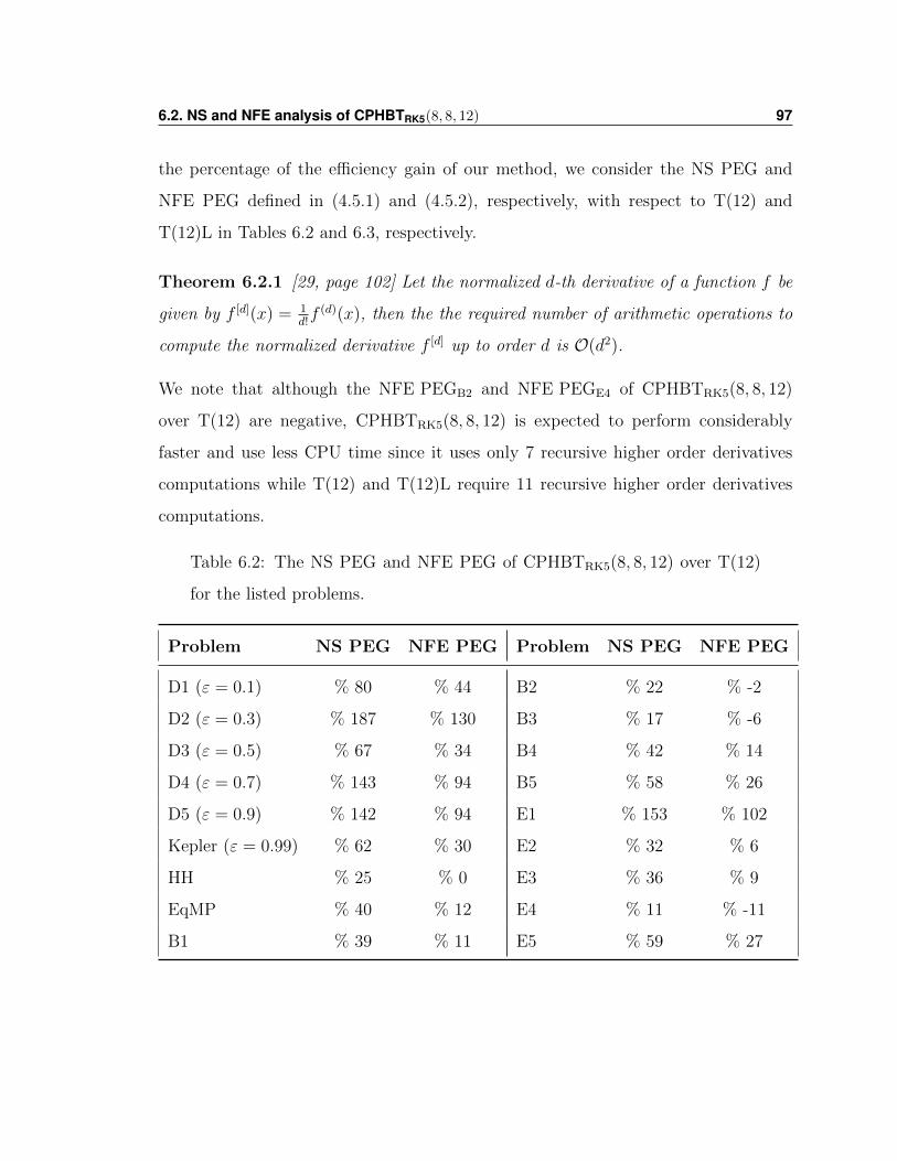
6.2. NS and NFE analysis of CPHBTRK5(8, 8, 12) 97
the percentage of the efficiency gain of our method, we consider the NS PEG and
NFE PEG defined in (4.5.1) and (4.5.2), respectively, with respect to T(12) and
T(12)L in Tables 6.2 and 6.3, respectively.
Theorem 6.2.1 [29, page 102] Let the normalized d-th derivative of a function f be
given by f [d](x) = 1d!f (d)(x), then the the required number of arithmetic operations to
compute the normalized derivative f [d] up to order d is O(d2).
We note that although the NFE PEGB2 and NFE PEGE4 of CPHBTRK5(8, 8, 12)
over T(12) are negative, CPHBTRK5(8, 8, 12) is expected to perform considerably
faster and use less CPU time since it uses only 7 recursive higher order derivatives
computations while T(12) and T(12)L require 11 recursive higher order derivatives
computations.
Table 6.2: The NS PEG and NFE PEG of CPHBTRK5(8, 8, 12) over T(12)
for the listed problems.
Problem NS PEG NFE PEG Problem NS PEG NFE PEG
D1 (ε = 0.1) % 80 % 44 B2 % 22 % -2
D2 (ε = 0.3) % 187 % 130 B3 % 17 % -6
D3 (ε = 0.5) % 67 % 34 B4 % 42 % 14
D4 (ε = 0.7) % 143 % 94 B5 % 58 % 26
D5 (ε = 0.9) % 142 % 94 E1 % 153 % 102
Kepler (ε = 0.99) % 62 % 30 E2 % 32 % 6
HH % 25 % 0 E3 % 36 % 9
EqMP % 40 % 12 E4 % 11 % -11
B1 % 39 % 11 E5 % 59 % 27
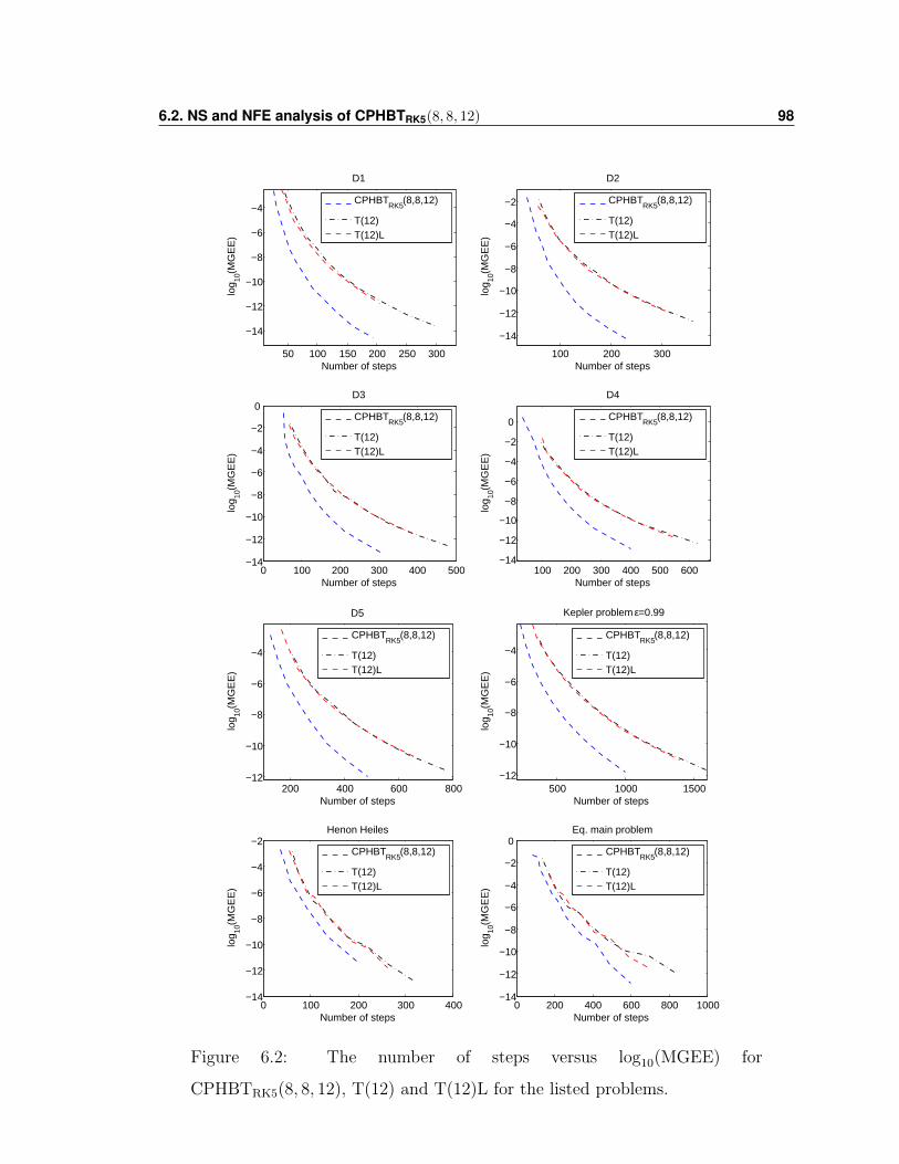
6.2. NS and NFE analysis of CPHBTRK5(8, 8, 12) 98
50 100 150 200 250 300
−14
−12
−10
−8
−6
−4
D1
Number of steps
log 10
(MG
EE
)
100 200 300
−14
−12
−10
−8
−6
−4
−2
D2
Number of steps
log 10
(MG
EE
)
0 100 200 300 400 500−14
−12
−10
−8
−6
−4
−2
0D3
Number of steps
log 10
(MG
EE
)
100 200 300 400 500 600−14
−12
−10
−8
−6
−4
−2
0
D4
Number of steps
log 10
(MG
EE
)
CPHBTRK5
(8,8,12)
T(12)T(12)L
CPHBTRK5
(8,8,12)
T(12)T(12)L
CPHBTRK5
(8,8,12)
T(12)T(12)L
CPHBTRK5
(8,8,12)
T(12)T(12)L
200 400 600 800−12
−10
−8
−6
−4
D5
Number of steps
log 10
(MG
EE
)
500 1000 1500−12
−10
−8
−6
−4
Kepler problem ε=0.99
Number of steps
log 10
(MG
EE
)
0 100 200 300 400−14
−12
−10
−8
−6
−4
−2Henon Heiles
Number of steps
log 10
(MG
EE
)
0 200 400 600 800 1000−14
−12
−10
−8
−6
−4
−2
0Eq. main problem
Number of steps
log 10
(MG
EE
)
CPHBTRK5
(8,8,12)
T(12)T(12)L
CPHBTRK5
(8,8,12)
T(12)T(12)L
CPHBTRK5
(8,8,12)
T(12)T(12)L
CPHBTRK5
(8,8,12)
T(12)T(12)L
Figure 6.2: The number of steps versus log10(MGEE) for
CPHBTRK5(8, 8, 12), T(12) and T(12)L for the listed problems.
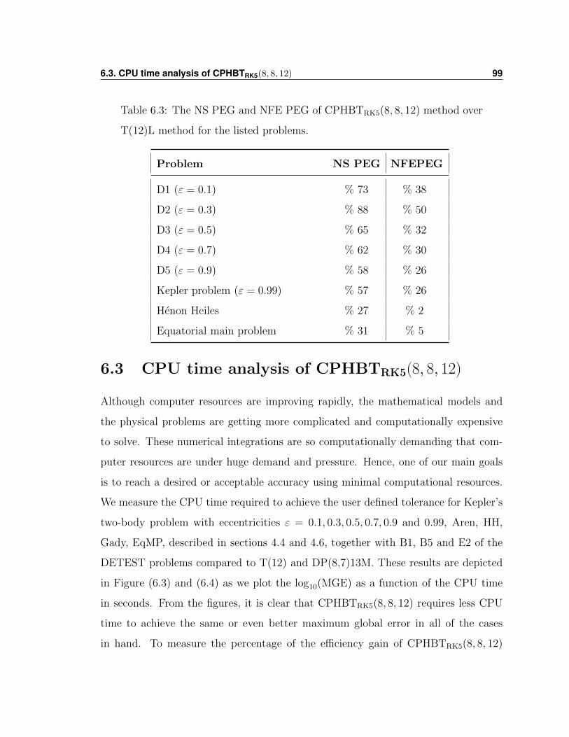
6.3. CPU time analysis of CPHBTRK5(8, 8, 12) 99
Table 6.3: The NS PEG and NFE PEG of CPHBTRK5(8, 8, 12) method over
T(12)L method for the listed problems.
Problem NS PEG NFEPEG
D1 (ε = 0.1) % 73 % 38
D2 (ε = 0.3) % 88 % 50
D3 (ε = 0.5) % 65 % 32
D4 (ε = 0.7) % 62 % 30
D5 (ε = 0.9) % 58 % 26
Kepler problem (ε = 0.99) % 57 % 26
Henon Heiles % 27 % 2
Equatorial main problem % 31 % 5
6.3 CPU time analysis of CPHBTRK5(8, 8, 12)
Although computer resources are improving rapidly, the mathematical models and
the physical problems are getting more complicated and computationally expensive
to solve. These numerical integrations are so computationally demanding that com-
puter resources are under huge demand and pressure. Hence, one of our main goals
is to reach a desired or acceptable accuracy using minimal computational resources.
We measure the CPU time required to achieve the user defined tolerance for Kepler’s
two-body problem with eccentricities ε = 0.1, 0.3, 0.5, 0.7, 0.9 and 0.99, Aren, HH,
Gady, EqMP, described in sections 4.4 and 4.6, together with B1, B5 and E2 of the
DETEST problems compared to T(12) and DP(8,7)13M. These results are depicted
in Figure (6.3) and (6.4) as we plot the log10(MGE) as a function of the CPU time
in seconds. From the figures, it is clear that CPHBTRK5(8, 8, 12) requires less CPU
time to achieve the same or even better maximum global error in all of the cases
in hand. To measure the percentage of the efficiency gain of CPHBTRK5(8, 8, 12)
6.3. CPU time analysis of CPHBTRK5(8, 8, 12) 100
over T(12), DP(8,7)13M and CPHBTRK4(9, 6, 12), we compute the CPU PEG for
all the consider test problems summarized in Table 6.4. As expected from analyz-
ing the Figures (6.3) and (6.4), CPHBTRK5(8, 8, 12) has large positive CPU PEG
over T(12) and DP(8,7)13M. However, the CPU PEG of CPHBTRK5(8, 8, 12) over
CPHBTRK4(9, 6, 12) is positive for 7 problems and negative for 6 problems. This
is a consequence of the direct function evaluations versus recursive computation of
higher order derivatives. In CPHBTRK5(8, 8, 12), we have 15 functions evaluations
composed of 8 direct function evaluations and 7 recursive computations of higher
order derivatives. While in CPHBTRK4(9, 6, 12), we have 14 functions evaluations
composed of 6 direct function evaluations and 8 recursive computations of higher or-
der derivatives. Since the computational complexity of the higher order derivatives is
quadratic [29, page 102], we expect that CPHBTRK4(9, 6, 12) will require more CPU
time compared to CPHBTRK5(8, 8, 12) when applied to problems with computation-
ally expensive functions. And for less expensive functions, CPHBTRK4(9, 6, 12) will
require less CPU time compared to CPHBTRK5(8, 8, 12).
Finally, we summarize some of the numerical results. In Table 6.5, we list the
CPU time, MGE, MGEE and NS of CPHBTRK5(8, 8, 12) and T(12) for the D-class
DETEST problems together with Kepler’s two-body problem with eccentricity ε =
0.99. Also, in Table 6.6, we list the CPU time, MGE and NS of both methods for
Arenstorf problem, Galactic dynamics problem together with B1, B5 and E2 of the
DETEST problems. We note the remarkable performance of CPHBTRK5(8, 8, 12)
compared to T(12). In all the considered problems, CPHBTRK5(8, 8, 12) requires less
integration steps to achieve better maximum global error and maximum global energy
error and still requires less CPU time although CPHBTRK5(8, 8, 12) has 15 function
evaluations per integration step while T(12) has only 12 function evaluations per
integration step.
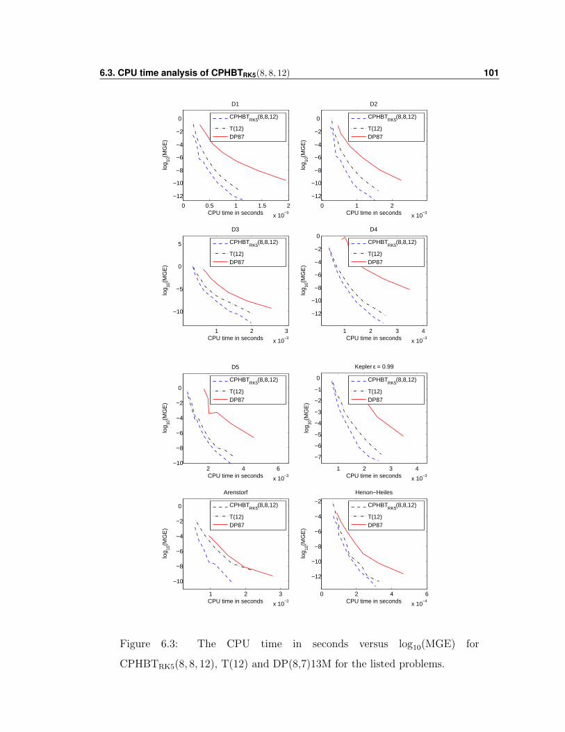
6.3. CPU time analysis of CPHBTRK5(8, 8, 12) 101
0 0.5 1 1.5 2
x 10−3
−12
−10
−8
−6
−4
−2
0
log 10
(MG
E)
CPU time in seconds
D1
CPHBT
RK5(8,8,12)
T(12)DP87
0 1 2
x 10−3
−12
−10
−8
−6
−4
−2
0
log 10
(MG
E)
CPU time in seconds
D2
CPHBT
RK5(8,8,12)
T(12)DP87
1 2 3
x 10−3
−10
−5
0
5
log 10
(MG
E)
CPU time in seconds
D3
CPHBT
RK5(8,8,12)
T(12)DP87
1 2 3 4
x 10−3
−12
−10
−8
−6
−4
−2
0
log 10
(MG
E)
CPU time in seconds
D4
CPHBT
RK5(8,8,12)
T(12)DP87
2 4 6
x 10−3
−10
−8
−6
−4
−2
0
log 10
(MG
E)
CPU time in seconds
D5
CPHBT
RK5(8,8,12)
T(12)DP87
1 2 3 4
x 10−3
−7
−6
−5
−4
−3
−2
−1
0
log 10
(MG
E)
CPU time in seconds
Kepler ε = 0.99
CPHBT
RK5(8,8,12)
T(12)DP87
1 2 3
x 10−3
−10
−8
−6
−4
−2
0
log 10
(MG
E)
CPU time in seconds
Arenstorf
CPHBT
RK5(8,8,12)
T(12)DP87
0 2 4 6
x 10−4
−12
−10
−8
−6
−4
−2
log 10
(MG
E)
CPU time in seconds
Henon−Heiles
CPHBT
RK5(8,8,12)
T(12)DP87
Figure 6.3: The CPU time in seconds versus log10(MGE) for
CPHBTRK5(8, 8, 12), T(12) and DP(8,7)13M for the listed problems.
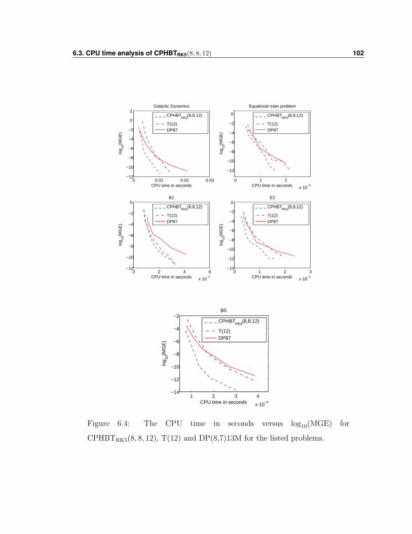
6.3. CPU time analysis of CPHBTRK5(8, 8, 12) 102
0 0.01 0.02 0.03−12
−10
−8
−6
−4
−2
0
2
log 10
(MG
E)
CPU time in seconds
Galactic Dynamics
CPHBT
RK5(8,8,12)
T(12)DP87
0 1 2
x 10−3
−12
−10
−8
−6
−4
−2
0
log 10
(MG
E)
CPU time in seconds
Equatorial main problem
CPHBT
RK5(8,8,12)
T(12)DP87
0 2 4 6
x 10−4
−12
−10
−8
−6
−4
−2
0
log 10
(MG
E)
CPU time in seconds
B1
CPHBT
RK5(8,8,12)
T(12)DP87
0 1 2 3
x 10−3
−14
−12
−10
−8
−6
−4
−2
0
log 10
(MG
E)
CPU time in seconds
E2
CPHBT
RK5(8,8,12)
T(12)DP87
1 2 3 4
x 10−4
−14
−12
−10
−8
−6
−4
−2
log 10
(MG
E)
CPU time in seconds
B5
CPHBT
RK5(8,8,12)
T(12)DP87
Figure 6.4: The CPU time in seconds versus log10(MGE) for
CPHBTRK5(8, 8, 12), T(12) and DP(8,7)13M for the listed problems.
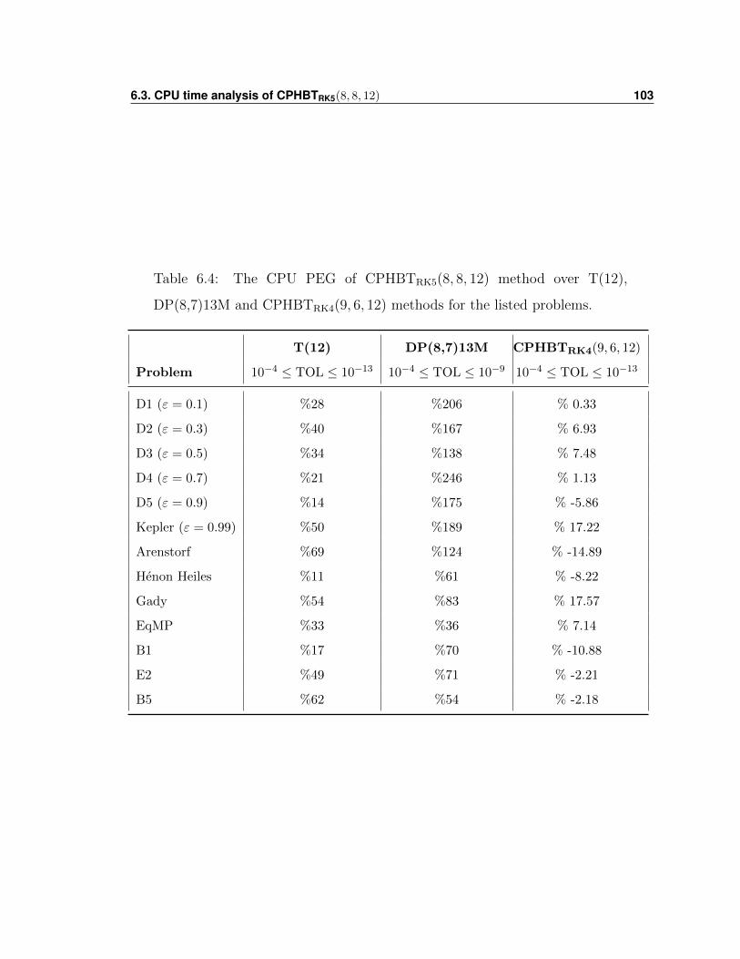
6.3. CPU time analysis of CPHBTRK5(8, 8, 12) 103
Table 6.4: The CPU PEG of CPHBTRK5(8, 8, 12) method over T(12),
DP(8,7)13M and CPHBTRK4(9, 6, 12) methods for the listed problems.
T(12) DP(8,7)13M CPHBTRK4(9, 6, 12)
Problem 10−4 ≤ TOL ≤ 10−13 10−4 ≤ TOL ≤ 10−9 10−4 ≤ TOL ≤ 10−13
D1 (ε = 0.1) %28 %206 % 0.33
D2 (ε = 0.3) %40 %167 % 6.93
D3 (ε = 0.5) %34 %138 % 7.48
D4 (ε = 0.7) %21 %246 % 1.13
D5 (ε = 0.9) %14 %175 % -5.86
Kepler (ε = 0.99) %50 %189 % 17.22
Arenstorf %69 %124 % -14.89
Henon Heiles %11 %61 % -8.22
Gady %54 %83 % 17.57
EqMP %33 %36 % 7.14
B1 %17 %70 % -10.88
E2 %49 %71 % -2.21
B5 %62 %54 % -2.18
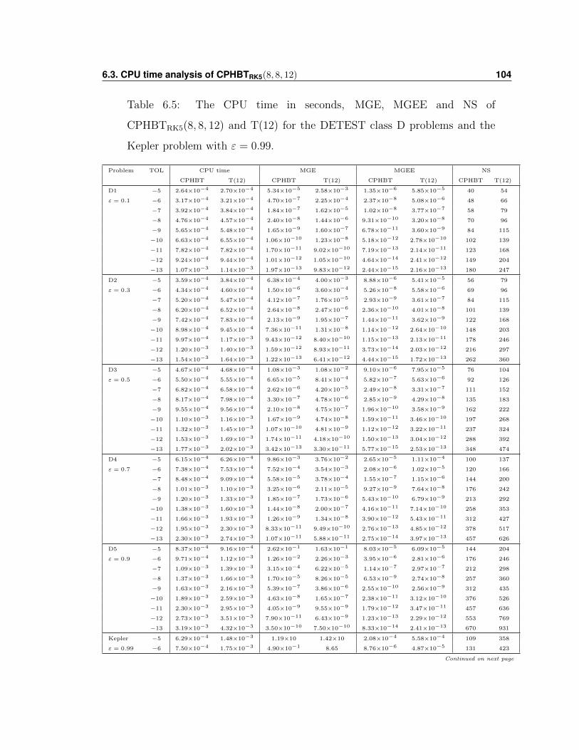
6.3. CPU time analysis of CPHBTRK5(8, 8, 12) 104
Table 6.5: The CPU time in seconds, MGE, MGEE and NS of
CPHBTRK5(8, 8, 12) and T(12) for the DETEST class D problems and the
Kepler problem with ε = 0.99.
Problem TOL CPU time MGE MGEE NS
CPHBT T(12) CPHBT T(12) CPHBT T(12) CPHBT T(12)
D1 −5 2.64×10⁻⁴ 2.70×10⁻⁴ 5.34×10⁻⁵ 2.58×10⁻³ 1.35×10⁻⁶ 5.85×10⁻⁵ 40 54
ε = 0.1 −6 3.17×10⁻⁴ 3.21×10⁻⁴ 4.70×10⁻⁷ 2.25×10⁻⁴ 2.37×10⁻⁸ 5.08×10⁻⁶ 48 66
−7 3.92×10⁻⁴ 3.84×10⁻⁴ 1.84×10⁻⁷ 1.62×10⁻⁵ 1.02×10⁻⁸ 3.77×10⁻⁷ 58 79
−8 4.76×10⁻⁴ 4.57×10⁻⁴ 2.40×10⁻⁸ 1.44×10⁻⁶ 9.31×10⁻¹⁰ 3.20×10⁻⁸ 70 96
−9 5.65×10⁻⁴ 5.48×10⁻⁴ 1.65×10⁻⁹ 1.60×10⁻⁷ 6.78×10⁻¹¹ 3.60×10⁻⁹ 84 115
−10 6.63×10⁻⁴ 6.55×10⁻⁴ 1.06×10⁻¹⁰ 1.23×10⁻⁸ 5.18×10⁻¹² 2.78×10⁻¹⁰ 102 139
−11 7.82×10⁻⁴ 7.82×10⁻⁴ 1.70×10⁻¹¹ 9.02×10⁻¹⁰ 7.19×10⁻¹³ 2.14×10⁻¹¹ 123 168
−12 9.24×10⁻⁴ 9.44×10⁻⁴ 1.01×10⁻¹² 1.05×10⁻¹⁰ 4.64×10⁻¹⁴ 2.41×10⁻¹² 149 204
−13 1.07×10⁻³ 1.14×10⁻³ 1.97×10⁻¹³ 9.83×10⁻¹² 2.44×10⁻¹⁵ 2.16×10⁻¹³ 180 247
D2 −5 3.59×10⁻⁴ 3.84×10⁻⁴ 6.38×10⁻⁴ 4.00×10⁻³ 8.88×10⁻⁶ 5.41×10⁻⁵ 56 79
ε = 0.3 −6 4.34×10⁻⁴ 4.60×10⁻⁴ 1.50×10⁻⁶ 3.60×10⁻⁴ 5.26×10⁻⁸ 5.58×10⁻⁶ 69 96
−7 5.20×10⁻⁴ 5.47×10⁻⁴ 4.12×10⁻⁷ 1.76×10⁻⁵ 2.93×10⁻⁹ 3.61×10⁻⁷ 84 115
−8 6.20×10⁻⁴ 6.52×10⁻⁴ 2.64×10⁻⁸ 2.47×10⁻⁶ 2.36×10⁻¹⁰ 4.01×10⁻⁸ 101 139
−9 7.42×10⁻⁴ 7.83×10⁻⁴ 2.13×10⁻⁹ 1.95×10⁻⁷ 1.44×10⁻¹¹ 3.62×10⁻⁹ 122 168
−10 8.98×10⁻⁴ 9.45×10⁻⁴ 7.36×10⁻¹¹ 1.31×10⁻⁸ 1.14×10⁻¹² 2.64×10⁻¹⁰ 148 203
−11 9.97×10⁻⁴ 1.17×10⁻³ 9.43×10⁻¹² 8.40×10⁻¹⁰ 1.15×10⁻¹³ 2.13×10⁻¹¹ 178 246
−12 1.20×10⁻³ 1.40×10⁻³ 1.59×10⁻¹² 8.93×10⁻¹¹ 3.73×10⁻¹⁴ 2.03×10⁻¹² 216 297
−13 1.54×10⁻³ 1.64×10⁻³ 1.22×10⁻¹³ 6.41×10⁻¹² 4.44×10⁻¹⁵ 1.72×10⁻¹³ 262 360
D3 −5 4.67×10⁻⁴ 4.68×10⁻⁴ 1.08×10⁻³ 1.08×10⁻² 9.10×10⁻⁶ 7.95×10⁻⁵ 76 104
ε = 0.5 −6 5.50×10⁻⁴ 5.55×10⁻⁴ 6.65×10⁻⁵ 8.41×10⁻⁴ 5.82×10⁻⁷ 5.63×10⁻⁶ 92 126
−7 6.82×10⁻⁴ 6.58×10⁻⁴ 2.62×10⁻⁶ 4.20×10⁻⁵ 2.49×10⁻⁸ 3.31×10⁻⁷ 111 152
−8 8.17×10⁻⁴ 7.98×10⁻⁴ 3.30×10⁻⁷ 4.78×10⁻⁶ 2.85×10⁻⁹ 4.29×10⁻⁸ 135 183
−9 9.55×10⁻⁴ 9.56×10⁻⁴ 2.10×10⁻⁸ 4.75×10⁻⁷ 1.96×10⁻¹⁰ 3.58×10⁻⁹ 162 222
−10 1.10×10⁻³ 1.16×10⁻³ 1.67×10⁻⁹ 4.74×10⁻⁸ 1.59×10⁻¹¹ 3.46×10⁻¹⁰ 197 268
−11 1.32×10⁻³ 1.45×10⁻³ 1.07×10⁻¹⁰ 4.81×10⁻⁹ 1.12×10⁻¹² 3.22×10⁻¹¹ 237 324
−12 1.53×10⁻³ 1.69×10⁻³ 1.74×10⁻¹¹ 4.18×10⁻¹⁰ 1.50×10⁻¹³ 3.04×10⁻¹² 288 392
−13 1.77×10⁻³ 2.02×10⁻³ 3.42×10⁻¹³ 3.30×10⁻¹¹ 5.77×10⁻¹⁵ 2.53×10⁻¹³ 348 474
D4 −5 6.15×10⁻⁴ 6.26×10⁻⁴ 9.86×10⁻³ 3.76×10⁻² 2.65×10⁻⁵ 1.11×10⁻⁴ 100 137
ε = 0.7 −6 7.38×10⁻⁴ 7.53×10⁻⁴ 7.52×10⁻⁴ 3.54×10⁻³ 2.08×10⁻⁶ 1.02×10⁻⁵ 120 166
−7 8.48×10⁻⁴ 9.09×10⁻⁴ 5.58×10⁻⁵ 3.78×10⁻⁴ 1.55×10⁻⁷ 1.15×10⁻⁶ 144 200
−8 1.01×10⁻³ 1.10×10⁻³ 3.25×10⁻⁶ 2.11×10⁻⁵ 9.27×10⁻⁹ 7.64×10⁻⁸ 176 242
−9 1.20×10⁻³ 1.33×10⁻³ 1.85×10⁻⁷ 1.73×10⁻⁶ 5.43×10⁻¹⁰ 6.79×10⁻⁹ 213 292
−10 1.38×10⁻³ 1.60×10⁻³ 1.44×10⁻⁸ 2.00×10⁻⁷ 4.16×10⁻¹¹ 7.14×10⁻¹⁰ 258 353
−11 1.66×10⁻³ 1.93×10⁻³ 1.26×10⁻⁹ 1.34×10⁻⁸ 3.90×10⁻¹² 5.43×10⁻¹¹ 312 427
−12 1.95×10⁻³ 2.30×10⁻³ 8.33×10⁻¹¹ 9.49×10⁻¹⁰ 2.76×10⁻¹³ 4.85×10⁻¹² 378 517
−13 2.30×10⁻³ 2.74×10⁻³ 1.07×10⁻¹¹ 5.88×10⁻¹¹ 2.75×10⁻¹⁴ 3.97×10⁻¹³ 457 626
D5 −5 8.37×10⁻⁴ 9.16×10⁻⁴ 2.62×10⁻¹ 1.63×10⁻¹ 8.03×10⁻⁵ 6.09×10⁻⁵ 144 204
ε = 0.9 −6 9.71×10⁻⁴ 1.12×10⁻³ 1.26×10⁻² 2.26×10⁻³ 3.95×10⁻⁶ 2.81×10⁻⁶ 176 246
−7 1.09×10⁻³ 1.39×10⁻³ 3.15×10⁻⁴ 6.22×10⁻⁵ 1.14×10⁻⁷ 2.97×10⁻⁷ 212 298
−8 1.37×10⁻³ 1.66×10⁻³ 1.70×10⁻⁵ 8.26×10⁻⁵ 6.53×10⁻⁹ 2.74×10⁻⁸ 257 360
−9 1.63×10⁻³ 2.16×10⁻³ 5.39×10⁻⁷ 3.86×10⁻⁶ 2.55×10⁻¹⁰ 2.56×10⁻⁹ 312 435
−10 1.89×10⁻³ 2.59×10⁻³ 4.63×10⁻⁸ 1.65×10⁻⁷ 2.38×10⁻¹¹ 3.12×10⁻¹⁰ 376 526
−11 2.30×10⁻³ 2.95×10⁻³ 4.05×10⁻⁹ 9.55×10⁻⁹ 1.79×10⁻¹² 3.47×10⁻¹¹ 457 636
−12 2.73×10⁻³ 3.51×10⁻³ 7.90×10⁻¹¹ 6.43×10⁻⁹ 1.23×10⁻¹³ 2.29×10⁻¹² 553 769
−13 3.19×10⁻³ 4.32×10⁻³ 3.50×10⁻¹⁰ 7.50×10⁻¹⁰ 8.33×10⁻¹⁴ 2.41×10⁻¹³ 670 931
Kepler −5 6.29×10⁻⁴ 1.48×10⁻³ 1.19×10 1.42×10 2.08×10⁻⁴ 5.58×10⁻⁴ 109 358
ε = 0.99 −6 7.50×10⁻⁴ 1.75×10⁻³ 4.90×10⁻¹ 8.65 8.76×10⁻⁶ 4.87×10⁻⁵ 131 423
Continued on next page
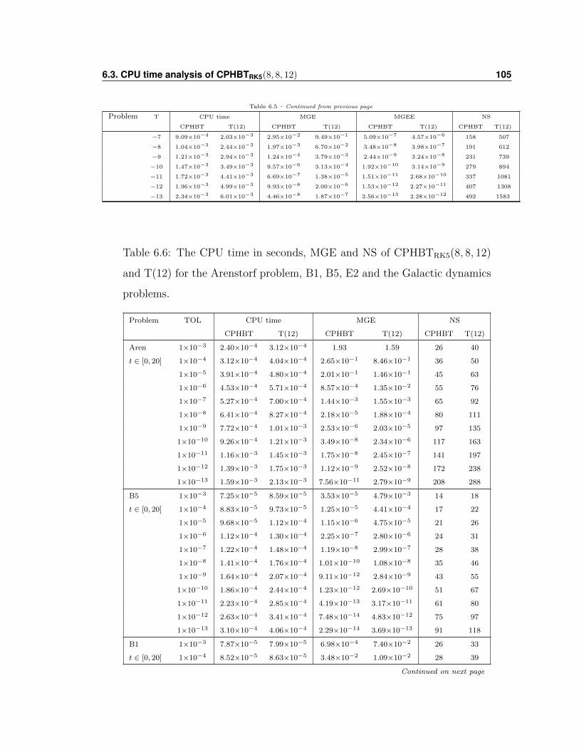
6.3. CPU time analysis of CPHBTRK5(8, 8, 12) 105
Table 6.5 – Continued from previous page
Problem T CPU time MGE MGEE NS
CPHBT T(12) CPHBT T(12) CPHBT T(12) CPHBT T(12)
−7 9.09×10⁻⁴ 2.03×10⁻³ 2.95×10⁻² 9.49×10⁻¹ 5.09×10⁻⁷ 4.57×10⁻⁶ 158 507
−8 1.04×10⁻³ 2.44×10⁻³ 1.97×10⁻³ 6.70×10⁻² 3.48×10⁻⁸ 3.98×10⁻⁷ 191 612
−9 1.21×10⁻³ 2.94×10⁻³ 1.24×10⁻⁴ 3.79×10⁻³ 2.44×10⁻⁹ 3.24×10⁻⁸ 231 739
−10 1.47×10⁻³ 3.49×10⁻³ 9.57×10⁻⁶ 3.13×10⁻⁴ 1.92×10⁻¹⁰ 3.14×10⁻⁹ 279 894
−11 1.72×10⁻³ 4.41×10⁻³ 6.69×10⁻⁷ 1.38×10⁻⁵ 1.51×10⁻¹¹ 2.68×10⁻¹⁰ 337 1081
−12 1.96×10⁻³ 4.99×10⁻³ 9.93×10⁻⁸ 2.00×10⁻⁶ 1.53×10⁻¹² 2.27×10⁻¹¹ 407 1308
−13 2.34×10⁻³ 6.01×10⁻³ 4.46×10⁻⁸ 1.87×10⁻⁷ 2.56×10⁻¹³ 2.28×10⁻¹² 492 1583
Table 6.6: The CPU time in seconds, MGE and NS of CPHBTRK5(8, 8, 12)
and T(12) for the Arenstorf problem, B1, B5, E2 and the Galactic dynamics
problems.
Problem TOL CPU time MGE NS
CPHBT T(12) CPHBT T(12) CPHBT T(12)
Aren 1×10⁻³ 2.40×10⁻⁴ 3.12×10⁻⁴ 1.93 1.59 26 40
t ∈ [0, 20] 1×10⁻⁴ 3.12×10⁻⁴ 4.04×10⁻⁴ 2.65×10⁻¹ 8.46×10⁻¹ 36 50
1×10⁻⁵ 3.91×10⁻⁴ 4.80×10⁻⁴ 2.01×10⁻¹ 1.46×10⁻¹ 45 63
1×10⁻⁶ 4.53×10⁻⁴ 5.71×10⁻⁴ 8.57×10⁻⁴ 1.35×10⁻² 55 76
1×10⁻⁷ 5.27×10⁻⁴ 7.00×10⁻⁴ 1.44×10⁻³ 1.55×10⁻³ 65 92
1×10⁻⁸ 6.41×10⁻⁴ 8.27×10⁻⁴ 2.18×10⁻⁵ 1.88×10⁻⁴ 80 111
1×10⁻⁹ 7.72×10⁻⁴ 1.01×10⁻³ 2.53×10⁻⁶ 2.03×10⁻⁵ 97 135
1×10⁻¹⁰ 9.26×10⁻⁴ 1.21×10⁻³ 3.49×10⁻⁸ 2.34×10⁻⁶ 117 163
1×10⁻¹¹ 1.16×10⁻³ 1.45×10⁻³ 1.75×10⁻⁸ 2.45×10⁻⁷ 141 197
1×10⁻¹² 1.39×10⁻³ 1.75×10⁻³ 1.12×10⁻⁹ 2.52×10⁻⁸ 172 238
1×10⁻¹³ 1.59×10⁻³ 2.13×10⁻³ 7.56×10⁻¹¹ 2.79×10⁻⁹ 208 288
B5 1×10⁻³ 7.25×10⁻⁵ 8.59×10⁻⁵ 3.53×10⁻⁵ 4.79×10⁻³ 14 18
t ∈ [0, 20] 1×10⁻⁴ 8.83×10⁻⁵ 9.73×10⁻⁵ 1.25×10⁻⁵ 4.41×10⁻⁴ 17 22
1×10⁻⁵ 9.68×10⁻⁵ 1.12×10⁻⁴ 1.15×10⁻⁶ 4.75×10⁻⁵ 21 26
1×10⁻⁶ 1.12×10⁻⁴ 1.30×10⁻⁴ 2.25×10⁻⁷ 2.80×10⁻⁶ 24 31
1×10⁻⁷ 1.22×10⁻⁴ 1.48×10⁻⁴ 1.19×10⁻⁸ 2.99×10⁻⁷ 28 38
1×10⁻⁸ 1.41×10⁻⁴ 1.76×10⁻⁴ 1.01×10⁻¹⁰ 1.08×10⁻⁸ 35 46
1×10⁻⁹ 1.64×10⁻⁴ 2.07×10⁻⁴ 9.11×10⁻¹² 2.84×10⁻⁹ 43 55
1×10⁻¹⁰ 1.86×10⁻⁴ 2.44×10⁻⁴ 1.23×10⁻¹² 2.69×10⁻¹⁰ 51 67
1×10⁻¹¹ 2.23×10⁻⁴ 2.85×10⁻⁴ 4.19×10⁻¹³ 3.17×10⁻¹¹ 61 80
1×10⁻¹² 2.63×10⁻⁴ 3.41×10⁻⁴ 7.48×10⁻¹⁴ 4.83×10⁻¹² 75 97
1×10⁻¹³ 3.10×10⁻⁴ 4.06×10⁻⁴ 2.29×10⁻¹⁴ 3.69×10⁻¹³ 91 118
B1 1×10⁻³ 7.87×10⁻⁵ 7.99×10⁻⁵ 6.98×10⁻⁴ 7.40×10⁻² 26 33
t ∈ [0, 20] 1×10⁻⁴ 8.52×10⁻⁵ 8.63×10⁻⁵ 3.48×10⁻² 1.09×10⁻² 28 39
Continued on next page
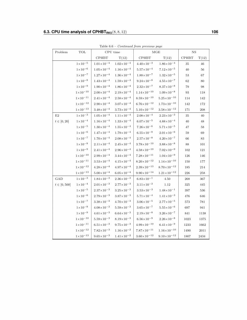
6.3. CPU time analysis of CPHBTRK5(8, 8, 12) 106
Table 6.6 – Continued from previous page
Problem TOL CPU time MGE NS
CPHBT T(12) CPHBT T(12) CPHBT T(12)
1×10⁻⁵ 1.01×10⁻⁴ 1.02×10⁻⁴ 4.40×10⁻³ 1.86×10⁻⁴ 35 46
1×10⁻⁶ 1.05×10⁻⁴ 1.16×10⁻⁴ 5.57×10⁻⁴ 7.12×10⁻⁵ 40 56
1×10⁻⁷ 1.27×10⁻⁴ 1.36×10⁻⁴ 1.88×10⁻⁷ 1.32×10⁻⁵ 53 67
1×10⁻⁸ 1.43×10⁻⁴ 1.59×10⁻⁴ 9.24×10⁻⁸ 4.55×10⁻⁷ 62 80
1×10⁻⁹ 1.90×10⁻⁴ 1.86×10⁻⁴ 2.32×10⁻⁷ 8.37×10⁻⁸ 79 98
1×10⁻¹⁰ 2.00×10⁻⁴ 2.19×10⁻⁴ 1.14×10⁻¹⁰ 1.09×10⁻⁸ 93 118
1×10⁻¹¹ 2.41×10⁻⁴ 2.58×10⁻⁴ 8.59×10⁻¹⁰ 5.25×10⁻¹⁰ 114 142
1×10⁻¹² 2.90×10⁻⁴ 3.07×10⁻⁴ 6.76×10⁻¹² 1.73×10⁻¹⁰ 142 172
1×10⁻¹³ 3.48×10⁻⁴ 3.73×10⁻⁴ 5.10×10⁻¹² 3.58×10⁻¹² 171 208
E2 1×10⁻³ 1.05×10⁻⁴ 1.11×10⁻⁴ 2.08×10⁻⁴ 2.23×10⁻³ 35 40
t ∈ [0, 20] 1×10⁻⁴ 1.16×10⁻⁴ 1.33×10⁻⁴ 6.07×10⁻⁵ 4.88×10⁻⁴ 40 48
1×10⁻⁵ 1.30×10⁻⁴ 1.55×10⁻⁴ 7.26×10⁻⁶ 5.71×10⁻⁵ 47 58
1×10⁻⁶ 1.47×10⁻⁴ 1.79×10⁻⁴ 6.55×10⁻⁸ 2.01×10⁻⁶ 59 69
1×10⁻⁷ 1.70×10⁻⁴ 2.08×10⁻⁴ 2.57×10⁻⁸ 4.20×10⁻⁷ 66 83
1×10⁻⁸ 2.11×10⁻⁴ 2.45×10⁻⁴ 3.78×10⁻¹⁰ 3.88×10⁻⁸ 88 101
1×10⁻⁹ 2.41×10⁻⁴ 2.96×10⁻⁴ 4.58×10⁻¹⁰ 7.02×10⁻⁹ 102 121
1×10⁻¹⁰ 2.99×10⁻⁴ 3.44×10⁻⁴ 7.28×10⁻¹¹ 1.04×10⁻⁹ 126 146
1×10⁻¹¹ 3.53×10⁻⁴ 4.15×10⁻⁴ 8.20×10⁻¹² 1.14×10⁻¹⁰ 150 177
1×10⁻¹² 4.28×10⁻⁴ 4.97×10⁻⁴ 2.39×10⁻¹³ 8.70×10⁻¹² 185 214
1×10⁻¹³ 5.00×10⁻⁴ 6.05×10⁻⁴ 9.90×10⁻¹⁴ 1.21×10⁻¹² 226 258
GAD 1×10⁻³ 1.84×10⁻³ 2.36×10⁻³ 6.83×10⁻¹ 4.50 268 367
t ∈ [0, 500] 1×10⁻⁴ 2.01×10⁻³ 2.77×10⁻³ 3.11×10⁻² 1.12 325 445
1×10⁻⁵ 2.37×10⁻³ 3.25×10⁻³ 3.53×10⁻³ 1.48×10⁻¹ 397 536
1×10⁻⁶ 2.79×10⁻³ 3.87×10⁻³ 5.71×10⁻⁴ 1.41×10⁻³ 476 646
1×10⁻⁷ 3.38×10⁻³ 4.70×10⁻³ 3.06×10⁻⁵ 2.77×10⁻⁵ 573 781
1×10⁻⁸ 4.08×10⁻³ 5.59×10⁻³ 3.65×10⁻⁷ 5.55×10⁻⁶ 697 941
1×10⁻⁹ 4.61×10⁻³ 6.64×10⁻³ 2.19×10⁻⁸ 3.26×10⁻⁷ 841 1138
1×10⁻¹⁰ 5.59×10⁻³ 8.19×10⁻³ 6.56×10⁻⁹ 2.26×10⁻⁸ 1023 1375
1×10⁻¹¹ 6.51×10⁻³ 9.75×10⁻³ 4.99×10⁻¹⁰ 6.41×10⁻⁹ 1233 1662
1×10⁻¹² 7.82×10⁻³ 1.16×10⁻² 7.87×10⁻¹¹ 1.16×10⁻¹⁰ 1490 2011
1×10⁻¹³ 9.65×10⁻³ 1.41×10⁻² 3.60×10⁻¹² 9.10×10⁻¹² 1807 2434
6.4. The propagation of error in a long-term integration problem for CPHBTRK5(8, 8, 12) 107
6.4 The propagation of error in a long-term inte-
gration problem for CPHBTRK5(8, 8, 12)
In the previous sections, we showed that CPHBTRK5(8, 8, 12) performs very well in
terms of NS, NFE, MGE, MGEE and CPU time required to solve several problems
often used to test higher-order ODE solvers. However, one of the main interests of
this work is the contractivity preserving property and the propagation of discretiza-
tion errors in long-term integration problems. Since in some astronomical simulation
problems, experts need to run the simulations for very large intervals, it is important
to use a numerical method that prevents or minimizes the propagation of discretiza-
tion errors to achieve satisfactory results. In the following subsections, we show that
CPHBTRK5(8, 8, 12) succeeds in achieving these properties.
6.4.1 Fixed step-size configuration
To be consistent with the previous chapters, we compare CPHBTRK5(8, 8, 12) in a
fixed step-size configurations to the Adams-Bashforth-Moulton method, ABM(12,11),
of order 12 with predictor of order 11 and corrector of order 12 in PECE mode and
CPHBTRK4(9, 6, 12) in fixed step-size configurations. The fixed step sizes hCPHBTRK5,
hCPHBTRK4and hABM are chosen so that all three methods use approximately equal
CPU time when applied to Kepler’s two-body problem with eccentricities ε = 0.3, 0.5
and 0.7 over the integrations interval t ∈ [0, 20000π]. We plot the energy error (
∆E(t) = E(t)−E(0)E(0)
) as a function of time in log-log scale using the MATLAB func-
tion loglog. We plot 300 equidistant points spanning the integration period and we
use the MATLAB filter command to remove some chattering. We plot the results
in Figure (6.5). We show that the fixed step size CPHBTRK5(8, 8, 12) performs re-
markably better than the fixed step size ABM(12,11) and CPHBTRK4(9, 6, 12). On
average, CPHBTRK5(8, 8, 12) is 40, 40 and 128 times more accurate that ABM(12,11)
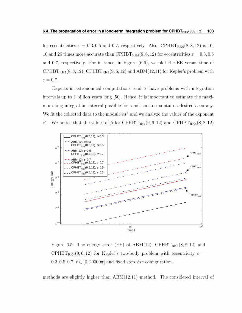
6.4. The propagation of error in a long-term integration problem for CPHBTRK5(8, 8, 12) 108
for eccentricities ε = 0.3, 0.5 and 0.7, respectively. Also, CPHBTRK5(8, 8, 12) is 10,
10 and 26 times more accurate than CPHBTRK4(9, 6, 12) for eccentricities ε = 0.3, 0.5
and 0.7, respectively. For instance, in Figure (6.6), we plot the EE versus time of
CPHBTRK5(8, 8, 12), CPHBTRK4(9, 6, 12) and ABM(12,11) for Kepler’s problem with
ε = 0.7.
Experts in astronomical computations tend to have problems with integration
intervals up to 1 billion years long [50]. Hence, it is important to estimate the maxi-
mum long-integration interval possible for a method to maintain a desired accuracy.
We fit the collected data to the module αtβ and we analyze the values of the exponent
β. We notice that the values of β for CPHBTRK4(9, 6, 12) and CPHBTRK5(8, 8, 12)
104
105
10−10
10−9
10−8
10−7
10−6
10−5
time t
Ene
rgy
Err
or
CPHBT
RK5(8,8,12), ε=0.3
ABM(12), ε=0.3CPHBT
RK5(8,8,12), ε=0.5
ABM(12), ε=0.5CPHBT
RK5(8,8,12), ε=0.7
ABM(12), ε=0.7CPHBT
RK4(9,6,12), ε=0.7
CPHBTRK4
(9,6,12), ε=0.5
CPHBTRK4
(9,6,12), ε=0.3
CPHBTRK4
CPHBTRK4
CPHBTRK4
Figure 6.5: The energy error (EE) of ABM(12), CPHBTRK5(8, 8, 12) and
CPHBTRK4(9, 6, 12) for Kepler’s two-body problem with eccentricity ε =
0.3, 0.5, 0.7, t ∈ [0, 20000π] and fixed step size configuration.
methods are slightly higher than ABM(12,11) method. The considered interval of
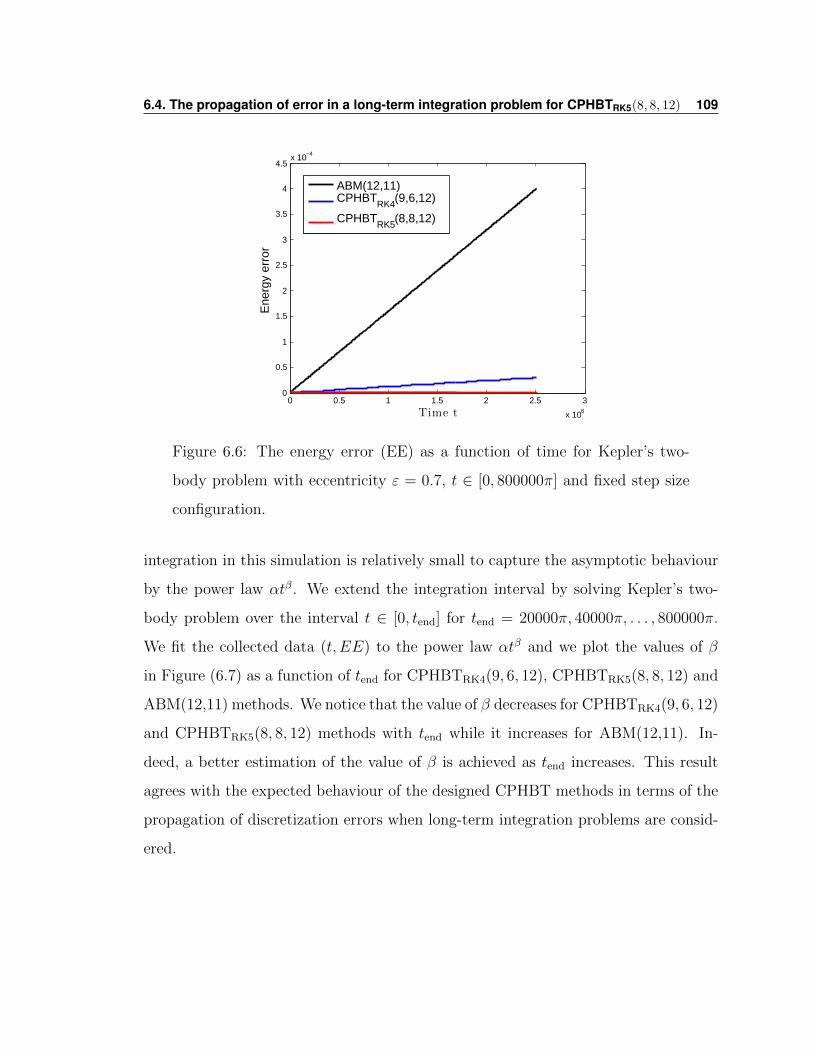
6.4. The propagation of error in a long-term integration problem for CPHBTRK5(8, 8, 12) 109
0 0.5 1 1.5 2 2.5 3
x 106
0
0.5
1
1.5
2
2.5
3
3.5
4
4.5x 10⁻⁴
Time t
Ene
rgy
erro
r
ABM(12,11)CPHBT
RK4(9,6,12)
CPHBTRK5
(8,8,12)
Figure 6.6: The energy error (EE) as a function of time for Kepler’s two-
body problem with eccentricity ε = 0.7, t ∈ [0, 800000π] and fixed step size
configuration.
integration in this simulation is relatively small to capture the asymptotic behaviour
by the power law αtβ. We extend the integration interval by solving Kepler’s two-
body problem over the interval t ∈ [0, tend] for tend = 20000π, 40000π, . . . , 800000π.
We fit the collected data (t, EE) to the power law αtβ and we plot the values of β
in Figure (6.7) as a function of tend for CPHBTRK4(9, 6, 12), CPHBTRK5(8, 8, 12) and
ABM(12,11) methods. We notice that the value of β decreases for CPHBTRK4(9, 6, 12)
and CPHBTRK5(8, 8, 12) methods with tend while it increases for ABM(12,11). In-
deed, a better estimation of the value of β is achieved as tend increases. This result
agrees with the expected behaviour of the designed CPHBT methods in terms of the
propagation of discretization errors when long-term integration problems are consid-
ered.
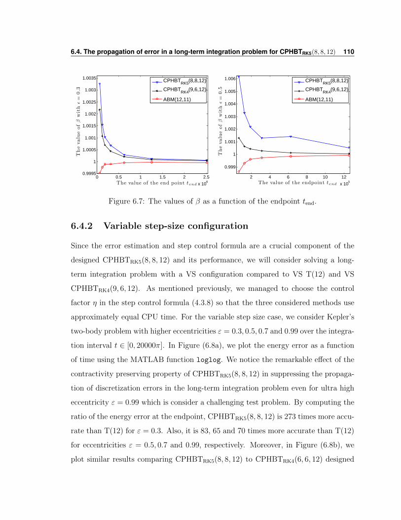
6.4. The propagation of error in a long-term integration problem for CPHBTRK5(8, 8, 12) 110
0 0.5 1 1.5 2 2.5
x 106
0.9995
1
1.0005
1.001
1.0015
1.002
1.0025
1.003
1.0035
The value of the end point tend
Thevalueofβ
withε=
0.3
CPHBT
RK5(8,8,12)
CPHBTRK4
(9,6,12)
ABM(12,11)
2 4 6 8 10 12
x 105
0.999
1
1.001
1.002
1.003
1.004
1.005
1.006
The value of the endpoint tend
Thevalueofβ
withε=
0.5
CPHBT
RK5(8,8,12)
CPHBTRK4
(9,6,12)
ABM(12,11)
Figure 6.7: The values of β as a function of the endpoint tend.
6.4.2 Variable step-size configuration
Since the error estimation and step control formula are a crucial component of the
designed CPHBTRK5(8, 8, 12) and its performance, we will consider solving a long-
term integration problem with a VS configuration compared to VS T(12) and VS
CPHBTRK4(9, 6, 12). As mentioned previously, we managed to choose the control
factor η in the step control formula (4.3.8) so that the three considered methods use
approximately equal CPU time. For the variable step size case, we consider Kepler’s
two-body problem with higher eccentricities ε = 0.3, 0.5, 0.7 and 0.99 over the integra-
tion interval t ∈ [0, 20000π]. In Figure (6.8a), we plot the energy error as a function
of time using the MATLAB function loglog. We notice the remarkable effect of the
contractivity preserving property of CPHBTRK5(8, 8, 12) in suppressing the propaga-
tion of discretization errors in the long-term integration problem even for ultra high
eccentricity ε = 0.99 which is consider a challenging test problem. By computing the
ratio of the energy error at the endpoint, CPHBTRK5(8, 8, 12) is 273 times more accu-
rate than T(12) for ε = 0.3. Also, it is 83, 65 and 70 times more accurate than T(12)
for eccentricities ε = 0.5, 0.7 and 0.99, respectively. Moreover, in Figure (6.8b), we
plot similar results comparing CPHBTRK5(8, 8, 12) to CPHBTRK4(6, 6, 12) designed
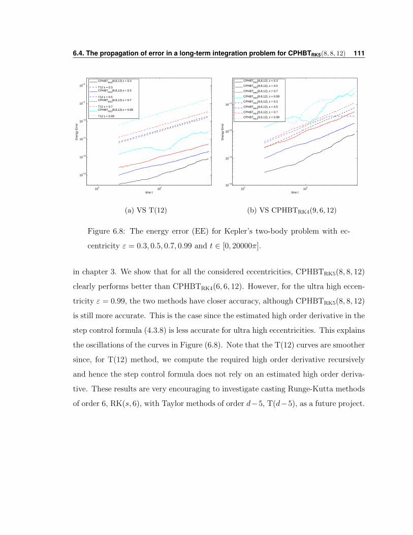
6.4. The propagation of error in a long-term integration problem for CPHBTRK5(8, 8, 12) 111
103
104
10−13
10−12
10−11
10−10
10−9
10−8
time t
Ene
rgy
Err
or
CPHBT
RK5(8,8,12) ε = 0.3
T12 ε = 0.3CPHBT
RK5(8,8,12) ε = 0.5
T12 ε = 0.5CPHBT
RK5(8,8,12) ε = 0.7
T12 ε = 0.7CPHBT
RK5(8,8,12) ε = 0.99
T12 ε = 0.99
(a) VS T(12)
103
104
10−14
10−13
10−12
10−11
time t
Ene
rgy
Err
or
CPHBT
RK5(8,8,12), ε = 0.3
CPHBTRK5
(8,8,12), ε = 0.5
CPHBTRK5
(8,8,12), ε = 0.7
CPHBTRK5
(8,8,12), ε = 0.99
CPHBTRK4
(9,6,12), ε = 0.3
CPHBTRK4
(9,6,12), ε = 0.5
CPHBTRK4
(9,6,12), ε = 0.7
CPHBTRK4
(9,6,12), ε = 0.99
(b) VS CPHBTRK4(9, 6, 12)
Figure 6.8: The energy error (EE) for Kepler’s two-body problem with ec-
centricity ε = 0.3, 0.5, 0.7, 0.99 and t ∈ [0, 20000π].
in chapter 3. We show that for all the considered eccentricities, CPHBTRK5(8, 8, 12)
clearly performs better than CPHBTRK4(6, 6, 12). However, for the ultra high eccen-
tricity ε = 0.99, the two methods have closer accuracy, although CPHBTRK5(8, 8, 12)
is still more accurate. This is the case since the estimated high order derivative in the
step control formula (4.3.8) is less accurate for ultra high eccentricities. This explains
the oscillations of the curves in Figure (6.8). Note that the T(12) curves are smoother
since, for T(12) method, we compute the required high order derivative recursively
and hence the step control formula does not rely on an estimated high order deriva-
tive. These results are very encouraging to investigate casting Runge-Kutta methods
of order 6, RK(s, 6), with Taylor methods of order d−5, T(d−5), as a future project.
6.4. The propagation of error in a long-term integration problem for CPHBTRK5(8, 8, 12) 112
6.4.3 CPHBTRK5(8, 8, 12) compared to Runge-Kutta-Nystrom
methods of order 12
In this section, we will consider the special second order system of non-stiff ordinary
differential equations of the form
y′′(x) = f(x, y(x)), where y(x0), y′(x0) are given. (6.4.1)
This second order ODE system can be transformed to a first order ODE without loss
of generality. However, many authors [13, 15, 12] have shown that it is more efficient
to use explicit s-stage Runge-Kutta-Nystrom pair, denoted by RKN(p, q)sM, given
by the two Runge-Kutta methods of orders q and p where p > q and often p = q + 1
or p = q + 2. The RKN(p, q)sM methods are described by the following formula
yn+1 = yn + hny′n + h2
n
s∑i=1
bigi, y′n+1 = y′n + hn
s∑i=1
b′igi, (6.4.2)
yn+1 = yn + hny′n + h2
n
s∑i=1
bigi, y′n+1 = y′n + hn
s∑i=1
b′igi, (6.4.3)
gi = f(xn + cihn, yn + cihny
′n + h2
n
i−1∑j=1
aijgj), i = 1, 2, . . . , s, (6.4.4)
where y0 = y(x0) and y′0 = y′(x0). These methods are integrated with a step control
formula given by
hn+1 = stfac hn
(TOL
‖σn+1‖∞
) 11+p
, (6.4.5)
where σn+1 = max|yn+1 − yn+1|, |y′n+1 − y′n+1|, TOL is the user defined tolerance
and stfac = 0.9 is a step control factor. These methods are widely used in astro-
nomical computations when the derivatives are computationally ”cheap” to evaluate
[49]. Several authors developed different optimal Runge-Kutta-Nystrom methods.
In 2013, Sharp et al. [49] presented a new optimal explicit 17 stages Runge-Kutta-
Nystrom pair of order 12, RKN(12,10)17M, with applications in the astronomical
simulations field. In our numerical comparison of different Runge-Kutta-Nystrom
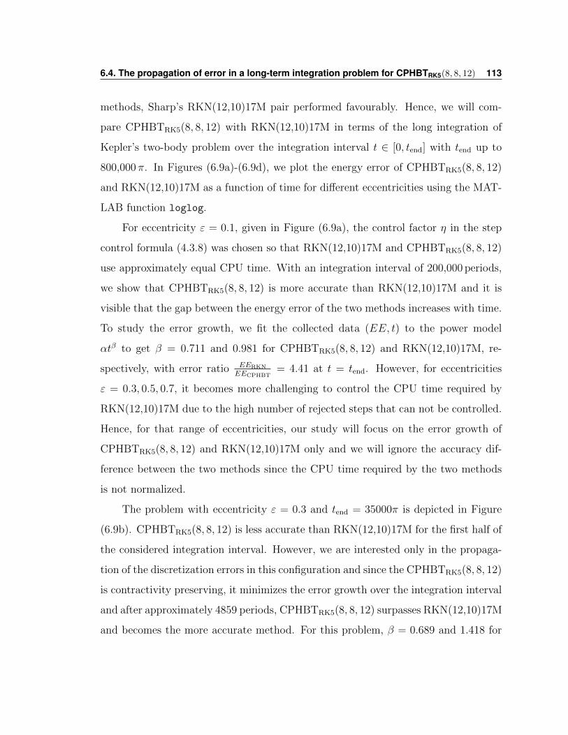
6.4. The propagation of error in a long-term integration problem for CPHBTRK5(8, 8, 12) 113
methods, Sharp’s RKN(12,10)17M pair performed favourably. Hence, we will com-
pare CPHBTRK5(8, 8, 12) with RKN(12,10)17M in terms of the long integration of
Kepler’s two-body problem over the integration interval t ∈ [0, tend] with tend up to
800,000π. In Figures (6.9a)-(6.9d), we plot the energy error of CPHBTRK5(8, 8, 12)
and RKN(12,10)17M as a function of time for different eccentricities using the MAT-
LAB function loglog.
For eccentricity ε = 0.1, given in Figure (6.9a), the control factor η in the step
control formula (4.3.8) was chosen so that RKN(12,10)17M and CPHBTRK5(8, 8, 12)
use approximately equal CPU time. With an integration interval of 200,000 periods,
we show that CPHBTRK5(8, 8, 12) is more accurate than RKN(12,10)17M and it is
visible that the gap between the energy error of the two methods increases with time.
To study the error growth, we fit the collected data (EE, t) to the power model
αtβ to get β = 0.711 and 0.981 for CPHBTRK5(8, 8, 12) and RKN(12,10)17M, re-
spectively, with error ratio EERKN
EECPHBT= 4.41 at t = tend. However, for eccentricities
ε = 0.3, 0.5, 0.7, it becomes more challenging to control the CPU time required by
RKN(12,10)17M due to the high number of rejected steps that can not be controlled.
Hence, for that range of eccentricities, our study will focus on the error growth of
CPHBTRK5(8, 8, 12) and RKN(12,10)17M only and we will ignore the accuracy dif-
ference between the two methods since the CPU time required by the two methods
is not normalized.
The problem with eccentricity ε = 0.3 and tend = 35000π is depicted in Figure
(6.9b). CPHBTRK5(8, 8, 12) is less accurate than RKN(12,10)17M for the first half of
the considered integration interval. However, we are interested only in the propaga-
tion of the discretization errors in this configuration and since the CPHBTRK5(8, 8, 12)
is contractivity preserving, it minimizes the error growth over the integration interval
and after approximately 4859 periods, CPHBTRK5(8, 8, 12) surpasses RKN(12,10)17M
and becomes the more accurate method. For this problem, β = 0.689 and 1.418 for
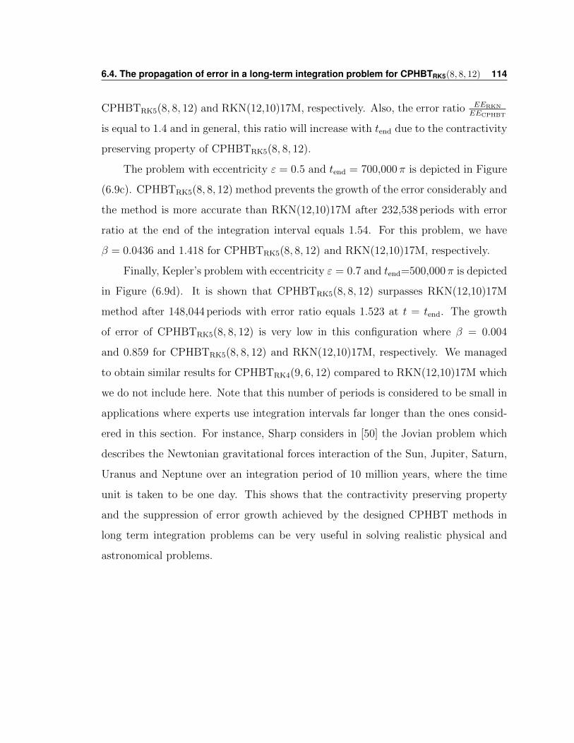
6.4. The propagation of error in a long-term integration problem for CPHBTRK5(8, 8, 12) 114
CPHBTRK5(8, 8, 12) and RKN(12,10)17M, respectively. Also, the error ratio EERKN
EECPHBT
is equal to 1.4 and in general, this ratio will increase with tend due to the contractivity
preserving property of CPHBTRK5(8, 8, 12).
The problem with eccentricity ε = 0.5 and tend = 700,000π is depicted in Figure
(6.9c). CPHBTRK5(8, 8, 12) method prevents the growth of the error considerably and
the method is more accurate than RKN(12,10)17M after 232,538 periods with error
ratio at the end of the integration interval equals 1.54. For this problem, we have
β = 0.0436 and 1.418 for CPHBTRK5(8, 8, 12) and RKN(12,10)17M, respectively.
Finally, Kepler’s problem with eccentricity ε = 0.7 and tend=500,000π is depicted
in Figure (6.9d). It is shown that CPHBTRK5(8, 8, 12) surpasses RKN(12,10)17M
method after 148,044 periods with error ratio equals 1.523 at t = tend. The growth
of error of CPHBTRK5(8, 8, 12) is very low in this configuration where β = 0.004
and 0.859 for CPHBTRK5(8, 8, 12) and RKN(12,10)17M, respectively. We managed
to obtain similar results for CPHBTRK4(9, 6, 12) compared to RKN(12,10)17M which
we do not include here. Note that this number of periods is considered to be small in
applications where experts use integration intervals far longer than the ones consid-
ered in this section. For instance, Sharp considers in [50] the Jovian problem which
describes the Newtonian gravitational forces interaction of the Sun, Jupiter, Saturn,
Uranus and Neptune over an integration period of 10 million years, where the time
unit is taken to be one day. This shows that the contractivity preserving property
and the suppression of error growth achieved by the designed CPHBT methods in
long term integration problems can be very useful in solving realistic physical and
astronomical problems.
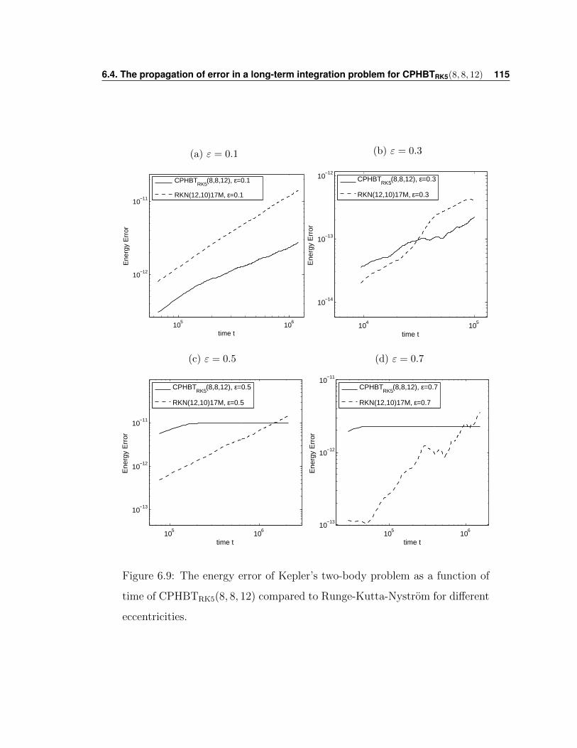
6.4. The propagation of error in a long-term integration problem for CPHBTRK5(8, 8, 12) 115
(a) ε = 0.1
105
106
10−12
10−11
time t
Ene
rgy
Err
or
CPHBT
RK5(8,8,12), ε=0.1
RKN(12,10)17M, ε=0.1
(b) ε = 0.3
104
105
10−14
10−13
10−12
time t
Ene
rgy
Err
or
CPHBT
RK5(8,8,12), ε=0.3
RKN(12,10)17M, ε=0.3
(c) ε = 0.5
105
106
10−13
10−12
10−11
time t
Ene
rgy
Err
or
CPHBT
RK5(8,8,12), ε=0.5
RKN(12,10)17M, ε=0.5
(d) ε = 0.7
105
106
10−13
10−12
10−11
time t
Ene
rgy
Err
or
CPHBT
RK5(8,8,12), ε=0.7
RKN(12,10)17M, ε=0.7
Figure 6.9: The energy error of Kepler’s two-body problem as a function of
time of CPHBTRK5(8, 8, 12) compared to Runge-Kutta-Nystrom for different
eccentricities.
Chapter 7
Conclusion and future work
In this thesis, we considered a new family of one-step, explicit, multi-derivative, multi-
stage, contractivity preserving, Hermite-Birkhoff-Taylor methods. The first set of
methods, CPHBTRK4(d, s, p), derived by casting s-stage Runge-Kutta methods of or-
der 4, RK(s,4), with Taylor method of order d, T(d), proved to be very efficient com-
pared to T(p), T(p)L by Martin Lara, DP(8,7)13M and ABM methods. In general,
the CPHBTRK4 is favourable in terms of the following comparison aspects: stability,
accuracy, efficiency and the propagation of discretization errors in long-term integra-
tion problems. We obtained the second set of methods, CPHBTRK5(p − 4, s, p), by
casting s-stage Runge-Kutta methods of order 5, RK(s,5), with the Taylor method
of order p − 4, T(p − 4). These methods are more challenging to obtain due to the
higher number of order conditions and contractivity preserving restrictions in the
optimization problem. CPHBTRK5 methods have larger regions of absolute stability
and perform better than CPHBTRK4 in terms of the NS, NFE percentage efficiency
gain. Also, on average, CPHBTRK4 and CPHBTRK5 require the same CPU time.
Since one of the main interests in this thesis is the contractivity preserving prop-
erty and the propagation of errors, we compare CPHBTRK5 to a well-known Runge-
Kutta-Nystrom pair, RKN, presented by Philip Sharp in 2013 [49]. CPHBTRK5 uti-
116
117
lizes the contractivity preserving property and performs better than the considered
RKN pair in terms of the propagation of discretization errors in the long-term in-
tegration of Kepler’s two-body problem where we consider integration intervals up
to t =800,000π. This result can be very interesting to experts in the field of astro-
nomical computations since they consider extremely large integration intervals, up
to t = 3.65242× 10¹¹ [50], and so the propagation of discretization errors is of great
importance. Since the main problem in the construction of the CPHBT methods
is the contractivity preserving property and the main problem in the construction
of the RKN methods is achieving maximum accuracy, the considered RKN method
had higher accuracy than CPHBT. However, in the considered long-term integration
problems, CPHBT surpasses RKN method in terms of accuracy after a relatively
small period of time.
The promising results in this work will be followed up by the following ideas that
will be addressed in our future work:
• The advantages of CPHBTRK5 over CPHBTRK4 in terms of stability, accuracy
and even the value of the contractivity preserving coefficients motivated us to
investigate a third set of CPHBT methods by casting s-stage Runge-Kutta
methods of order 6, RK(s,6), with Taylor method of order p − 5, T(p − 5).
Although such methods will be more complex to derive due to the higher number
of constraints in the optimization problem, we believe that such methods exist
and will have better stability and accuracy properties. Also, by construction,
these methods will require less higher order derivatives compared to CPHBTRK5
and CPHBTRK4 which will increase their computational efficiency.
• Since the main drawback of methods using higher order derivative information
is that we need to formulate and code the recurrence formulas of the higher
order derivatives described in Section 2.2.1 for each problem. This issue can be
solved by integrating the designed methods with some modern general purpose
118
algebraic manipulator similar to the work done by Lara, Elipe and Palacios’s in
[34], and Jorba and Zou’s in [29]. This will result in an application that takes
the differential equation as an input and provides a FORTRAN or C++ code as
an output with the recurrence formulas of the automatic differentiation process.
• We believe that the performance and stability of the RKN pair can be improved
by adding higher order derivative information. Such methods can be thought
of as combining two Hermite-Birkhoff-Taylor methods to create a pair of HBT
methods. Such methods can be divided into two categories:
1. CPHBTpq pair where we consider two contractivity preserving HBT meth-
ods of orders p and q with p = q+ 1 or p = q+ 2 and use a step controller
similar to RKN methods in (6.4.5). Such methods estimate the error more
accurately and allow a better automatic step-size control. Moreover, these
methods add minimal computational cost since the same function and
higher order derivatives are used for both methods.
2. Non-CP high accuracy HBT pair composed of two HBT methods designed
by choosing the free parameters specifically to minimize the principal er-
ror and achieve better accuracy. This special consideration of the free
parameters will be possible by dropping the large number of contractivity
preserving conditions in the optimization problem.
Appendices
119
Appendix A
CPHBTRK4(d, s, p) formulae
A.1 Five stages CPHBTRK4(d, 5, p) methods formu-
lae
CPHBTRK4(2,5,5) with ccp = 1.0625338959788060, and abscissa vector
σ = [0 4.2850362365796774×10⁻¹ 6.5248338991294597×10⁻¹ 6.0260786608926109×10⁻¹ 9.4283575658959828×10⁻¹]T .
Y2 = yn + 4.2850362365796774× 10⁻¹hnfn + 9.1807677744004626× 10⁻²h2ny(2)n ,
Y3 = yn + 2.4783303603362317× 10⁻¹hnfn + 4.0465035387932280× 10⁻¹hnF2 + 3.9473144104375933× 10⁻²h2ny(2)n ,
Y4 = yn + 3.0711977059612233× 10⁻¹hnfn + 8.8846520080429953× 10⁻²hnF2 + 2.0664157541270883× 10⁻¹hnF3
+8.6668687102258411× 10⁻³h2ny(2)n ,
Y5 = yn + 2.0871142715810950× 10⁻¹hnfn + 5.2743466069405748× 10⁻²hnF2 + 1.2267214191931065× 10⁻¹hnF3
+5.5870872144277239× 10⁻¹hnF4 + 5.1450602154364091× 10⁻³h2ny(2)n ,
yn+1 = yn + 2.5075377432281282× 10⁻¹hnfn + 2.0839397966111808× 10⁻¹hnF2 + 6.4981764618288446× 10⁻²hnF3
+2.9595862644754489× 10⁻¹hnF4 + 1.7991185495023562× 10⁻¹hnF5 + 2.0328576290332894× 10⁻²h2ny(2)n .
CPHBTRK4(3,5,5) with ccp = 1.6544514297191719, and abscissa vector
σ = [0 5.4808274228565224×10⁻¹ 6.3139226452853348×10⁻¹ 5.9512887026466110×10⁻¹ 8.7603815620983694×10⁻¹]T .
Y2 = yn + 5.4808274228565224× 10⁻¹hfn + 1.5019734619568034× 10⁻¹h2y(2)n + 9.7913207802001970× 10⁻³h3y
(3)n ,
Y3 = yn + 3.8116145601471918× 10⁻¹hfn + 2.5023080851381441× 10⁻¹hF2 + 6.2180908118627441× 10⁻²h2y(2)n
+1.3438194283833214× 10⁻²h3y(3)n ,
120
A.1. Five stages CPHBTRK4(d, 5, p) methods formulae 121
Y4 = yn + 3.3460998717488410× 10⁻¹hfn + 7.6275703390041152× 10⁻²hF2 + 1.8424317969973586× 10⁻¹hF3
+1.8954070972911352× 10⁻²h2y(2)n + 1.3566189439262331× 10⁻²h3y
(3)n ,
Y5 = yn + 2.5774902310335085× 10⁻¹hfn + 5.4523963216387562× 10⁻²hF2 + 1.3170207426930505× 10⁻¹hF3
+4.3206309562079354× 10⁻¹hF4 + 1.3548889391988866× 10⁻²h2y(2)n + 1.0825240235151289× 10⁻²h3y
(3)n ,
yn+1 = yn + 4.0368154940504869× 10⁻¹hfn + 7.1984917418738248× 10⁻²hF2 + 5.9113253061746168× 10⁻²hF3
+1.9392750836898545× 10⁻¹hF4 + 2.7129277174548150× 10⁻¹hF5 + 7.0147979821784903× 10⁻²h2y(2)n
+5.6284771897167256× 10⁻³h3y(3)n .
CPHBTRK4(3,5,6) with ccp= 6.8211668346068355×10⁻¹, and abscissa vector
σ = [0 4.7866009264327564×10⁻¹ 6.8440248420931726×10⁻¹ 6.8225905894506400×10⁻¹ 9.6045235789866867×10⁻¹]T .
Y2 = yn + 4.7866009264327564× 10⁻¹hnfn + 1.1455774214463461× 10⁻¹h2ny(2)n + 1.8278073155985095× 10⁻²h3ny
(3)n ,
Y3 = yn + 2.6377998718488588× 10⁻¹hnfn + 4.2062249702443144× 10⁻¹hnF2 + 3.2868176802382097× 10⁻²h2ny(2)n
+5.2442281844169098× 10⁻³h3ny(3)n ,
Y4 = yn + 4.3058405574487157× 10⁻¹hnfn + 5.6110204779506276× 10⁻²hnF2 + 1.9556479842068614× 10⁻¹hnF3
+7.2035962075298554× 10⁻²h2ny(2)n + 6.9956961270428622× 10⁻⁴h3ny
(3)n ,
Y5 = yn + 3.1787654927202391× 10⁻¹hnfn + 2.0990314695794404× 10⁻²hnF2 + 7.3159003400556089× 10⁻²hnF3
+5.4842649053029424× 10⁻¹hnF4 + 2.6947994920294642× 10⁻²h2ny(2)n + 4.8578091073209944× 10⁻⁴h3ny
(3)n ,
yn+1 = yn + 3.3737569831798614× 10⁻¹hnfn + 1.8139912869065516× 10⁻¹hnF2 + 4.0662218957669478× 10⁻²hnF3
+3.0481877832632642× 10⁻¹hnF4 + 1.3574417570736286× 10⁻¹hnF5 + 4.7000966108577895× 10⁻²h2ny(2)n
+2.8097543373721955× 10⁻³h3ny(3)n
CPHBTRK4(4,5,6) with ccp = 1.6289806645490685, and abscissa vector
σ = [0 6.0466839315262999×10⁻¹ 6.8897630604729898×10⁻¹ 6.6703533001073756×10⁻¹ 8.8273882977431872×10⁻¹]T .
Y2 = yn + 6.0466839315262999× 10⁻¹hnfn + 1.8281193283889177× 10⁻¹h2ny(2)n + 3.6846865892939729× 10⁻²h3ny
(3)n
+1.0708970275330335× 10⁻⁵h4ny(4)n ,
Y3 = yn + 4.6451021267513215× 10⁻¹hnfn + 2.2446609337216683× 10⁻¹hnF2 + 1.0161662315069432× 10⁻¹h2ny(2)n
+1.3473090632113511× 10⁻²h3ny(3)n + 2.3322068777870491× 10⁻³h4ny
(4)n ,
Y4 = yn + 4.5990915568820728× 10⁻¹hnfn + 5.5457713234330748× 10⁻²hnF2 + 1.5166846108819954× 10⁻¹hnF3
+8.4438563327518451× 10⁻²h2ny(2)n + 3.3287290094947950× 10⁻³h3ny
(3)n + 3.8749278184591696× 10⁻³h4ny
(4)n ,
Y5 = yn + 3.7679653094714194× 10⁻¹hnfn + 3.4175595121912289× 10⁻²hnF2 + 9.3465085677299234× 10⁻²hnF3
+3.7830161802796525× 10⁻¹hnF4 + 5.2213244509045596× 10⁻²h2ny(2)n + 2.0513160075384253× 10⁻³h3ny
(3)n
+2.5907000696281622× 10⁻³h4ny(4)n ,
yn+1 = yn + 5.0933497961429763× 10⁻¹hnfn + 3.9695675606679123× 10⁻²hnF2 + 3.8824652749983236× 10⁻²hnF3
+1.5714348142153173× 10⁻¹hnF4 + 2.5500121060750836× 10⁻¹hnF5 + 1.1932828954879460× 10⁻¹h2ny(2)n
A.1. Five stages CPHBTRK4(d, 5, p) methods formulae 122
+1.5883590473209471× 10⁻²h3ny(3)n + 1.0807291773231296× 10⁻³h4ny
(4)n .
CPHBTRK4(5,5,7) with ccp = 1.5486363112234323, and abscissa vector
σ = [0 5.9448263083486175×10⁻¹ 7.4611168636626923×10⁻¹ 7.1527878030425218×10⁻¹ 8.9279153752926677×10⁻¹]T .
Y2 = yn + 5.9448263083486175× 10⁻¹hnfn + 1.7670479918216928× 10⁻¹h2ny(2)n + 3.5015977966320645× 10⁻²h3ny
(3)n
+5.2040976756684626× 10⁻³h4ny(4)n + 5.9507643942744467× 10⁻⁴h5ny
(5)n ,
Y3 = yn + 4.4634974224850704× 10⁻¹hnfn + 2.9976194411776214× 10⁻¹hnF2 + 1.0013805510285899× 10⁻¹h2ny(2)n
+1.6255197473429017× 10⁻²h3ny(3)n + 2.4158578353375188× 10⁻³h4ny
(4)n + 4.2386402042934049× 10⁻⁴h5ny
(5)n ,
Y4 = yn + 5.3628836349796449× 10⁻¹hnfn + 5.6747759257548616× 10⁻²hnF2 + 1.2224265754873902× 10⁻¹hnF3
+1.3086963418977443× 10⁻¹h2ny(2)n + 1.6939482097573323× 10⁻²h3ny
(3)n + 4.5734464140764362× 10⁻⁴h4ny
(4)n
+2.1457557270600997× 10⁻⁴h5ny(5)n ,
Y5 = yn + 4.6032156704749760× 10⁻¹hnfn + 2.9757623371333759× 10⁻²hnF2 + 6.4102107481229298× 10⁻²hnF3
+3.3861023962920611× 10⁻¹hnF4 + 9.0819923799791646× 10⁻²h2ny(2)n + 8.8827952849606998× 10⁻³h3ny
(3)n
+3.4009877667845440× 10⁻⁴h4ny(4)n + 1.6672900302383718× 10⁻⁴h5ny
(5)n .
yn+1 = yn + 5.7497384573678145× 10⁻¹hnfn + 3.2441120753385122× 10⁻²hnF2 + 2.4932874462414000× 10⁻²hnF3
+1.3170435307193448× 10⁻¹hnF4 + 2.3594780597548484× 10⁻¹hnF5 + 1.5725407467662181× 10⁻¹h2ny(2)n
+2.6268526463189373× 10⁻²h3ny(3)n + 2.7874661505894647× 10⁻³h4ny
(4)n + 1.6007340660752472× 10⁻⁴h5ny
(5)n .
CPHBTRK4(6,5,8) with ccp = 1.4715349175532293, and abscissa vector
σ = [0 6.3812458308410325×10⁻¹ 7.6732516263606776×10⁻¹ 7.5421376503889004×10⁻¹ 9.0470574170528428×10⁻¹]T .
Y2 = yn + 6.3812458308410325× 10⁻¹hnfn + 2.0360149176813030× 10⁻¹h2ny(2)n + 4.3307705683279879× 10⁻²h3ny
(3)n
+6.9089279083680054× 10⁻³h4ny(4)n + 8.8175134821709183× 10⁻⁴h5ny
(5)n + 1.2838317254671800× 10⁻⁴h6ny
(6)n ,
Y3 = yn + 4.9720293695307349× 10⁻¹hnfn + 2.7012222568299432× 10⁻¹hnF2 + 1.2202231996152318× 10⁻¹h2ny(2)n
+2.0301341079021675× 10⁻²h3ny(3)n + 2.7462593735600987× 10⁻³h4ny
(4)n + 3.5049112355876980× 10⁻⁴h5ny
(5)n
+9.9487210341961491× 10⁻⁵h6ny(6)n ,
Y4 = yn + 5.9370283825951065× 10⁻¹hnfn + 4.5654695694174262× 10⁻²hnF2 + 1.1485623108520505× 10⁻¹hnF3
+1.6715374183417167× 10⁻¹h2ny(2)n + 2.8395948317622623× 10⁻²h3ny
(3)n + 2.8566635028080207× 10⁻³h4ny
(4)n
+5.9238241315113858× 10⁻⁵h5ny(5)n + 1.6833518626430792× 10⁻⁵h6ny
(6)n ,
Y5 = yn + 5.2693740981356185× 10⁻¹hnfn + 2.0530226230123742× 10⁻²hnF2 + 5.1649110179471089× 10⁻²hnF3
+3.0558899548212765× 10⁻¹hnF4 + 1.2603430877803559× 10⁻¹h2ny(2)n + 1.7115259039665234× 10⁻²h3ny
(3)n
+1.2845983766675317× 10⁻³h4ny(4)n + 4.2784131142800703× 10⁻⁵h5ny
(5)n + 4.5316048150476212× 10⁻⁵h6ny
(6)n ,
yn+1 = yn + 6.2838771624152567× 10⁻¹hnfn + 2.2913478782924837× 10⁻²hnF2 + 1.9961417389470458× 10⁻²hnF3
+1.1810444492173085× 10⁻¹hnF4 + 2.1063294266434826× 10⁻¹hnF5 + 1.9042461736685512× 10⁻¹h2ny(2)n
+3.6333015991553086× 10⁻²h3ny(3)n + 4.7308596338484195× 10⁻³h4ny
(4)n + 4.1480659453566184× 10⁻⁴h5ny
(5)n
A.1. Five stages CPHBTRK4(d, 5, p) methods formulae 123
+2.0390815678371275× 10⁻⁵h6ny(6)n .
CPHBTRK4(7,5,9) with ccp = 1.4115607214001771, and abscissa vector
σ = [0 6.7264209027272404×10⁻¹ 7.8570115394476325×10⁻¹ 7.8339576219887797×10⁻¹ 9.1412683756610613×10⁻¹]T .
Y2 = yn + 6.7264209027272404× 10⁻¹hnfn + 2.2622369080322974× 10⁻¹h2ny(2)n + 5.0722525417031622× 10⁻²h3ny
(3)n
+8.5295263801058816× 10⁻³h4ny(4)n + 1.1474636906701524× 10⁻³h5ny
(5)n + 1.2863872923407095× 10⁻⁴h6ny
(6)n
+1.6871283691865543× 10⁻⁵h7ny(7)n ,
Y3 = yn + 5.3985006213700604× 10⁻¹hnfn + 2.4585109180775722× 10⁻¹hnF2 + 1.4329335936566504× 10⁻¹h2ny(2)n
+2.5221656768449830× 10⁻²h3ny(3)n + 3.4086352785824706× 10⁻³h4ny
(4)n + 3.9820862126158530× 10⁻⁴h5ny
(5)n
+4.4641979895002042× 10⁻⁵h6ny(6)n + 5.8549048724342979× 10⁻⁶h7ny
(7)n ,
Y4 = yn + 6.3712202767851545× 10⁻¹hnfn + 3.7684224334290320× 10⁻²hnF2 + 1.0858951018607231× 10⁻¹hnF3
+1.9618756122956357× 10⁻¹h2ny(2)n + 3.8086849790783764× 10⁻²h3ny
(3)n + 5.0035703763330226× 10⁻³h4ny
(4)n
+4.1310702391352867× 10⁻⁴h5ny(5)n + 6.8427533622897276× 10⁻⁶h6ny
(6)n + 8.9746839854607379× 10⁻⁷h7ny
(7)n ,
Y5 = yn + 5.7925228138991269× 10⁻¹hnfn + 1.4764652723196561× 10⁻²hnF2 + 4.2545294101237273× 10⁻²hnF3
+2.7756460935175958× 10⁻¹hnF4 + 1.5701178533660620× 10⁻¹h2ny(2)n + 2.5667427335795582× 10⁻²h3ny
(3)n
+2.6654164614515119× 10⁻³h4ny(4)n + 1.6185504288187001× 10⁻⁴h5ny
(5)n + 4.8332984267274632× 10⁻⁶h6ny
(6)n
+3.5162749957115332× 10⁻⁷h7ny(7)n .
yn+1 = yn + 6.6992609764748168× 10⁻¹hnfn + 1.6928908398811920× 10⁻²hnF2 + 1.6276124483944193× 10⁻²hnF3
+1.0618509589795518× 10⁻¹hnF4 + 1.9068377357180699× 10⁻¹hnF5 + 2.1833062483429713× 10⁻¹h2ny(2)n
+4.5559398104867747× 10⁻²h3ny(3)n + 6.7074212297902388× 10⁻³h4ny
(4)n + 7.1620368169263062× 10⁻⁴h5ny
(5)n
+5.3466285655376258× 10⁻⁵h6ny(6)n + 2.2949248887023122× 10⁻⁶h7ny
(7)n .
CPHBTRK4(8,5,10) with ccp = 1.3638646257964513, and abscissa vector
σ = [0 7.0080215042708205×10⁻¹ 8.0155292312263227×10⁻¹ 8.0617794551281863×10⁻¹ 9.2177638433749054×10⁻¹]T .
Y2 = yn + 7.0080215042708205× 10⁻¹hnfn + 2.4556182702161131× 10⁻¹h2ny(2)n + 5.7363418813182784× 10⁻²h3ny
(3)n
+1.0050101815031959× 10⁻²h4ny(4)n + 1.4086265927971036× 10⁻³h5ny
(5)n + 1.6452809089683067× 10⁻⁴h6ny
(6)n
+1.6471662843737338× 10⁻⁵h7ny(7)n + 1.3780368036111647× 10⁻⁶h8ny
(8)n ,
Y3 = yn + 5.7598930912692958× 10⁻¹hnfn + 2.2556361399570268× 10⁻¹hnF2 + 1.6316807853692550× 10⁻¹h2ny(2)n
+3.0441420822447194× 10⁻²h3ny(3)n + 4.2604690652900757× 10⁻³h4ny
(4)n + 4.9033569512550257× 10⁻⁴h5ny
(5)n
+5.0615131326159361× 10⁻⁵h6ny(6)n + 5.0673132682173783× 10⁻⁶h7ny
(7)n + 4.2393680864481340× 10⁻⁷h8ny
(8)n ,
Y4 = yn + 6.7134687083218469× 10⁻¹hnfn + 3.1720695085314318× 10⁻²hnF2 + 1.0311037959531959× 10⁻¹hnF3
+2.2008308241789187× 10⁻¹h2ny(2)n + 4.6412646367557459× 10⁻²h3ny
(3)n + 6.9302909374724855× 10⁻³h4ny
(4)n
+7.4549437034508953× 10⁻⁴h5ny(5)n + 5.2301785173365859× 10⁻⁵h6ny
(6)n + 7.1260916703504024× 10⁻⁷h7ny
(7)n
+3.7931187385561651× 10⁻⁷h8ny(8)n ,
A.1. Five stages CPHBTRK4(d, 5, p) methods formulae 124
Y5 = yn + 6.2138885317264780× 10⁻¹hnfn + 1.0977009014961151× 10⁻²hnF2 + 3.5681549956889096× 10⁻²hnF3
+2.5372897219299267× 10⁻¹hnF4 + 1.8399178764908977× 10⁻¹h2ny(2)n + 3.3924417553441152× 10⁻²h3ny
(3)n
+4.2316163710359516× 10⁻³h4ny(4)n + 3.5592113113033997× 10⁻⁴h5ny
(5)n + 1.8099135778786784× 10⁻⁵h6ny
(6)n
+4.9543809927693444× 10⁻⁷h7ny(7)n + 6.7811743002780728× 10⁻⁷h8ny
(8)n ,
yn+1 = yn + 7.0321426874850679× 10⁻¹hnfn + 1.2920781087526969× 10⁻²hnF2 + 1.3481818905558848× 10⁻²hnF3
+9.5868258479031063× 10⁻²hnF4 + 1.7451487277937641× 10⁻¹hnF5 + 2.4198813337169503× 10⁻¹h2ny(2)n
+5.3869206897701916× 10⁻²h3ny(3)n + 8.6163531919612318× 10⁻³h4ny
(4)n + 1.0347489795011107× 10⁻³h5ny
(5)n
+9.3680192323108188× 10⁻⁵h6ny(6)n + 6.0871403686808235× 10⁻⁶h7ny
(7)n + 2.3175101190842453× 10⁻⁷h8ny
(8)n .
CPHBTRK4(9,5,11) with ccp = 1.3253079734478708, and abscissa vector
σ = [0 7.2429567207324930×10⁻¹ 8.1528856428413632×10⁻¹ 8.2450162786848580×10⁻¹ 9.2812027230881411×10⁻¹]T .
Y2 = yn + 7.2429567207324930× 10⁻¹hnfn + 2.6230211029201994× 10⁻¹h2ny(2)n + 6.3328094420063374× 10⁻²h3ny
(3)n
+1.1467066177274499× 10⁻²h4ny(4)n + 1.6611092807154917× 10⁻³h5ny
(5)n + 2.0052237714382313× 10⁻⁴h6ny
(6)n
+2.0748212845587281× 10⁻⁵h7ny(7)n + 1.8784800959141834× 10⁻⁶h8ny
(8)n + 6.1629758220391547× 10⁻³²h9ny
(9)n ,
Y3 = yn + 6.0694710911169403× 10⁻¹hnfn + 2.0834145517244243× 10⁻¹hnF2 + 1.8144690723140125× 10⁻¹h2ny(2)n
+3.5671362222369919× 10⁻²h3ny(3)n + 5.2153006558404869× 10⁻³h4ny
(4)n + 6.1269157584519765× 10⁻⁴h5ny
(5)n
+6.1805077935152860× 10⁻⁵h6ny(6)n + 5.7289258156145483× 10⁻⁶h7ny
(7)n + 5.1867952173481764× 10⁻⁷h8ny
(8)n
+4.8361850237535367× 10⁻⁸h9ny(9)n ,
Y4 = yn + 6.9914916425821572× 10⁻¹hnfn + 2.7122831285393719× 10⁻²hnF2 + 9.8229632324876429× 10⁻²hnF3
+2.4017102195620088× 10⁻¹h2ny(2)n + 5.3655667295174354× 10⁻²h3ny
(3)n + 8.6657866470045818× 10⁻³h4ny
(4)n
+1.0558933168246529× 10⁻³h5ny(5)n + 9.6416084843446254× 10⁻⁵h6ny
(6)n + 5.8887917418002241× 10⁻⁶h7ny
(7)n
+6.7524041561148269× 10⁻⁸h8ny(8)n + 6.3108523635658873× 10⁻⁹h9ny
(9)n ,
Y5 = yn + 6.5601718623534822× 10⁻¹hnfn + 8.3876075469791270× 10⁻³hnF2 + 3.0377050120939483× 10⁻²hnF3
+2.3333842840554728× 10⁻¹hnF4 + 2.0747453644503186× 10⁻¹h2ny(2)n + 4.1640348954393273× 10⁻²h3ny
(3)n
+5.8451373697182120× 10⁻³h4ny(4)n + 5.9060465527598365× 10⁻⁴h5ny
(5)n + 4.1732461687485503× 10⁻⁵h6ny
(6)n
+1.8210810464844811× 10⁻⁶h7ny(7)n + 4.6434535379714043× 10⁻⁸h8ny
(8)n + 8.3766562521193928× 10⁻⁸h9ny
(9)n ,
yn+1 = yn + 7.3049821038076390× 10⁻¹hnfn + 1.0112276063254677× 10⁻²hnF2 + 1.1320389876402904× 10⁻²hnF3
+8.6956500782500348× 10⁻²hnF4 + 1.6111262289707823× 10⁻¹hnF5 + 2.6221866991856319× 10⁻¹h2ny(2)n
+6.1303457437452448× 10⁻²h3ny(3)n + 1.0412678352601583× 10⁻²h4ny
(4)n + 1.3533693769707648× 10⁻³h5ny
(5)n
+1.3736913097097669× 10⁻⁴h6ny(6)n + 1.0797188914801632× 10⁻⁵h7ny
(7)n + 6.2101845671912387× 10⁻⁷h8ny
(8)n
+2.1237133463449921× 10⁻⁸h9ny(9)n .
CPHBTRK4(10,5,12) with ccp = 1.2936747608596961, and abscissa vector
σ = [0 7.4423533270870701×10⁻¹ 8.2727137725735045×10⁻¹ 8.3958210167620639×10⁻¹ 9.3347415242277998×10⁻¹]T .
Y2 = yn + 7.4423533270870701× 10⁻¹hnfn + 2.7694311522601994× 10⁻¹h2ny(2)n + 6.8703617167207562× 10⁻²h3ny
(3)n
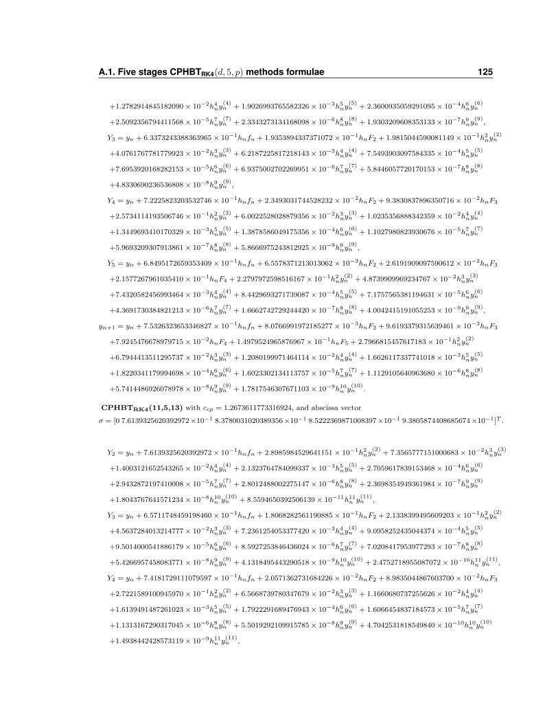
A.1. Five stages CPHBTRK4(d, 5, p) methods formulae 125
+1.2782914845182090× 10⁻²h4ny(4)n + 1.9026993765582326× 10⁻³h5ny
(5)n + 2.3600935059291095× 10⁻⁴h6ny
(6)n
+2.5092356794411568× 10⁻⁵h7ny(7)n + 2.3343273134168098× 10⁻⁶h8ny
(8)n + 1.9303209608353133× 10⁻⁷h9ny
(9)n ,
Y3 = yn + 6.3373243388363965× 10⁻¹hnfn + 1.9353894337371072× 10⁻¹hnF2 + 1.9815044590081149× 10⁻¹h2ny(2)n
+4.0761767781779923× 10⁻²h3ny(3)n + 6.2187225817218143× 10⁻³h4ny
(4)n + 7.5493903097584335× 10⁻⁴h5ny
(5)n
+7.6953920168282153× 10⁻⁵h6ny(6)n + 6.9375002702269951× 10⁻⁶h7ny
(7)n + 5.8446057720170153× 10⁻⁷h8ny
(8)n
+4.8330690236536808× 10⁻⁸h9ny(9)n ,
Y4 = yn + 7.2225823203532746× 10⁻¹hnfn + 2.3493031744528232× 10⁻²hnF2 + 9.3830837896350716× 10⁻²hnF3
+2.5734114193506746× 10⁻¹h2ny(2)n + 6.0022528028879356× 10⁻²h3ny
(3)n + 1.0235356888342359× 10⁻²h4ny
(4)n
+1.3449693410170329× 10⁻³h5ny(5)n + 1.3878586049175356× 10⁻⁴h6ny
(6)n + 1.1027980823930676× 10⁻⁵h7ny
(7)n
+5.9693209307913861× 10⁻⁷h8ny(8)n + 5.8666975243812925× 10⁻⁹h9ny
(9)n ,
Y5 = yn + 6.8495172659353409× 10⁻¹hnfn + 6.5578371213013062× 10⁻³hnF2 + 2.6191909097590612× 10⁻²hnF3
+2.1577267961035410× 10⁻¹hnF4 + 2.2797972598516167× 10⁻¹h2ny(2)n + 4.8739909969234767× 10⁻²h3ny
(3)n
+7.4320582456993464× 10⁻³h4ny(4)n + 8.4429693271739087× 10⁻⁴h5ny
(5)n + 7.1757565381194631× 10⁻⁵h6ny
(6)n
+4.3691730384821213× 10⁻⁶h7ny(7)n + 1.6662742729244420× 10⁻⁷h8ny
(8)n + 4.0042415191055253× 10⁻⁹h9ny
(9)n ,
yn+1 = yn + 7.5326323653346827× 10⁻¹hnfn + 8.0766991972185277× 10⁻³hnF2 + 9.6193379315639461× 10⁻³hnF3
+7.9245476678979715× 10⁻²hnF4 + 1.4979524965876967× 10⁻¹hnF5 + 2.7966815457617183× 10⁻¹h2ny(2)n
+6.7944413511295737× 10⁻²h3ny(3)n + 1.2080199971464114× 10⁻²h4ny
(4)n + 1.6626117337741018× 10⁻³h5ny
(5)n
+1.8220341179994698× 10⁻⁴h6ny(6)n + 1.6023302134113757× 10⁻⁵h7ny
(7)n + 1.1129105640963680× 10⁻⁶h8ny
(8)n
+5.7414486926078978× 10⁻⁸h9ny(9)n + 1.7817546307671103× 10⁻⁹h10n y
(10)n .
CPHBTRK4(11,5,13) with ccp = 1.2673611773316924, and abscissa vector
σ = [0 7.6139325620392972×10⁻¹ 8.3780031020389356×10⁻¹ 8.5222369871008397×10⁻¹ 9.3805874408685674×10⁻¹]T .
Y2 = yn + 7.6139325620392972× 10⁻¹hnfn + 2.8985984529641151× 10⁻¹h2ny(2)n + 7.3565777151000683× 10⁻²h3ny
(3)n
+1.4003121652543265× 10⁻²h4ny(4)n + 2.1323764784099337× 10⁻³h5ny
(5)n + 2.7059617839153468× 10⁻⁴h6ny
(6)n
+2.9432872197410008× 10⁻⁵h7ny(7)n + 2.8012488002275147× 10⁻⁶h8ny
(8)n + 2.3698354949361984× 10⁻⁷h9ny
(9)n
+1.8043767641571234× 10⁻⁸h10n y(10)n + 8.5594650392506139× 10⁻¹¹h11n y
(11)n ,
Y3 = yn + 6.5711748459198460× 10⁻¹hnfn + 1.8068282561190885× 10⁻¹hnF2 + 2.1338399495609203× 10⁻¹h2ny(2)n
+4.5637284013214777× 10⁻²h3ny(3)n + 7.2361254053377420× 10⁻³h4ny
(4)n + 9.0958252435044374× 10⁻⁴h5ny
(5)n
+9.5014000541886179× 10⁻⁵h6ny(6)n + 8.5927253846436024× 10⁻⁶h7ny
(7)n + 7.0208417953977293× 10⁻⁷h8ny
(8)n
+5.4266957458083771× 10⁻⁸h9ny(9)n + 4.1318495443290518× 10⁻⁹h10n y
(10)n + 2.4752718955087072× 10⁻¹⁰h11n y
(11)n ,
Y4 = yn + 7.4181729111079597× 10⁻¹hnfn + 2.0571362731684226× 10⁻²hnF2 + 8.9835044867603700× 10⁻²hnF3
+2.7221589100945970× 10⁻¹h2ny(2)n + 6.5668739780347679× 10⁻²h3ny
(3)n + 1.1660680737255626× 10⁻²h4ny
(4)n
+1.6139491487261023× 10⁻³h5ny(5)n + 1.7922291689476943× 10⁻⁴h6ny
(6)n + 1.6066454837184573× 10⁻⁵h7ny
(7)n
+1.1313167290317045× 10⁻⁶h8ny(8)n + 5.5019292109915785× 10⁻⁸h9ny
(9)n + 4.7042531818549840× 10⁻¹⁰h10n y
(10)n
+1.4938442428573119× 10⁻⁹h11n y(11)n ,
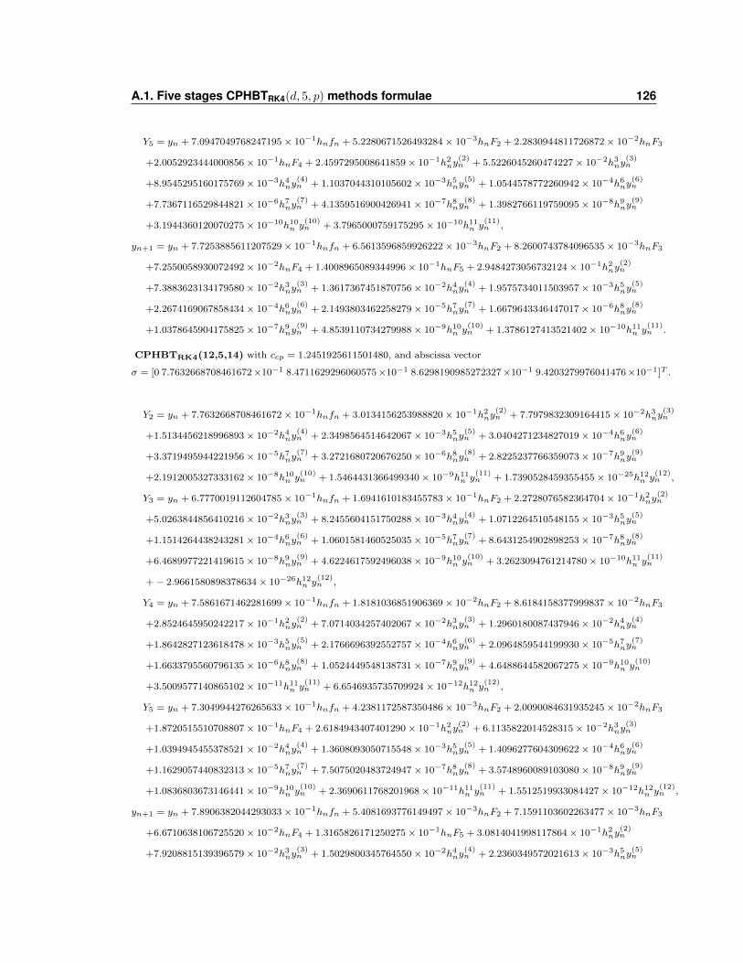
A.1. Five stages CPHBTRK4(d, 5, p) methods formulae 126
Y5 = yn + 7.0947049768247195× 10⁻¹hnfn + 5.2280671526493284× 10⁻³hnF2 + 2.2830944811726872× 10⁻²hnF3
+2.0052923444000856× 10⁻¹hnF4 + 2.4597295008641859× 10⁻¹h2ny(2)n + 5.5226045260474227× 10⁻²h3ny
(3)n
+8.9545295160175769× 10⁻³h4ny(4)n + 1.1037044310105602× 10⁻³h5ny
(5)n + 1.0544578772260942× 10⁻⁴h6ny
(6)n
+7.7367116529844821× 10⁻⁶h7ny(7)n + 4.1359516900426941× 10⁻⁷h8ny
(8)n + 1.3982766119759095× 10⁻⁸h9ny
(9)n
+3.1944360120070275× 10⁻¹⁰h10n y(10)n + 3.7965000759175295× 10⁻¹⁰h11n y
(11)n ,
yn+1 = yn + 7.7253885611207529× 10⁻¹hnfn + 6.5613596859926222× 10⁻³hnF2 + 8.2600743784096535× 10⁻³hnF3
+7.2550058930072492× 10⁻²hnF4 + 1.4008965089344996× 10⁻¹hnF5 + 2.9484273056732124× 10⁻¹h2ny(2)n
+7.3883623134179580× 10⁻²h3ny(3)n + 1.3617367451870756× 10⁻²h4ny
(4)n + 1.9575734011503957× 10⁻³h5ny
(5)n
+2.2674169067858434× 10⁻⁴h6ny(6)n + 2.1493803462258279× 10⁻⁵h7ny
(7)n + 1.6679643346447017× 10⁻⁶h8ny
(8)n
+1.0378645904175825× 10⁻⁷h9ny(9)n + 4.8539110734279988× 10⁻⁹h10n y
(10)n + 1.3786127413521402× 10⁻¹⁰h11n y
(11)n .
CPHBTRK4(12,5,14) with ccp = 1.2451925611501480, and abscissa vector
σ = [0 7.7632668708461672×10⁻¹ 8.4711629296060575×10⁻¹ 8.6298190985272327×10⁻¹ 9.4203279976041476×10⁻¹]T .
Y2 = yn + 7.7632668708461672× 10⁻¹hnfn + 3.0134156253988820× 10⁻¹h2ny(2)n + 7.7979832309164415× 10⁻²h3ny
(3)n
+1.5134456218996893× 10⁻²h4ny(4)n + 2.3498564514642067× 10⁻³h5ny
(5)n + 3.0404271234827019× 10⁻⁴h6ny
(6)n
+3.3719495944221956× 10⁻⁵h7ny(7)n + 3.2721680720676250× 10⁻⁶h8ny
(8)n + 2.8225237766359073× 10⁻⁷h9ny
(9)n
+2.1912005327333162× 10⁻⁸h10n y(10)n + 1.5464431366499340× 10⁻⁹h11n y
(11)n + 1.7390528459355455× 10⁻²⁵h12n y
(12)n ,
Y3 = yn + 6.7770019112604785× 10⁻¹hnfn + 1.6941610183455783× 10⁻¹hnF2 + 2.2728076582364704× 10⁻¹h2ny(2)n
+5.0263844856410216× 10⁻²h3ny(3)n + 8.2455604151750288× 10⁻³h4ny
(4)n + 1.0712264510548155× 10⁻³h5ny
(5)n
+1.1514264438243281× 10⁻⁴h6ny(6)n + 1.0601581460525035× 10⁻⁵h7ny
(7)n + 8.6431254902898253× 10⁻⁷h8ny
(8)n
+6.4689977221419615× 10⁻⁸h9ny(9)n + 4.6224617592496038× 10⁻⁹h10n y
(10)n + 3.2623094761214780× 10⁻¹⁰h11n y
(11)n
+− 2.9661580898378634× 10⁻²⁶h12n y(12)n ,
Y4 = yn + 7.5861671462281699× 10⁻¹hnfn + 1.8181036851906369× 10⁻²hnF2 + 8.6184158377999837× 10⁻²hnF3
+2.8524645950242217× 10⁻¹h2ny(2)n + 7.0714034257402067× 10⁻²h3ny
(3)n + 1.2960180087437946× 10⁻²h4ny
(4)n
+1.8642827123618478× 10⁻³h5ny(5)n + 2.1766696392552757× 10⁻⁴h6ny
(6)n + 2.0964859544199930× 10⁻⁵h7ny
(7)n
+1.6633795560796135× 10⁻⁶h8ny(8)n + 1.0524449548138731× 10⁻⁷h9ny
(9)n + 4.6488644582067275× 10⁻⁹h10n y
(10)n
+3.5009577140865102× 10⁻¹¹h11n y(11)n + 6.6546935735709924× 10⁻¹²h12n y
(12)n ,
Y5 = yn + 7.3049944276265633× 10⁻¹hnfn + 4.2381172587350486× 10⁻³hnF2 + 2.0090084631935245× 10⁻²hnF3
+1.8720515510708807× 10⁻¹hnF4 + 2.6184943407401290× 10⁻¹h2ny(2)n + 6.1135822014528315× 10⁻²h3ny
(3)n
+1.0394945455378521× 10⁻²h4ny(4)n + 1.3608093050715548× 10⁻³h5ny
(5)n + 1.4096277604309622× 10⁻⁴h6ny
(6)n
+1.1629057440832313× 10⁻⁵h7ny(7)n + 7.5075020483724947× 10⁻⁷h8ny
(8)n + 3.5748960089103080× 10⁻⁸h9ny
(9)n
+1.0836803673146441× 10⁻⁹h10n y(10)n + 2.3690611768201968× 10⁻¹¹h11n y
(11)n + 1.5512519933084427× 10⁻¹²h12n y
(12)n ,
yn+1 = yn + 7.8906382044293033× 10⁻¹hnfn + 5.4081693776149497× 10⁻³hnF2 + 7.1591103602263477× 10⁻³hnF3
+6.6710638106725520× 10⁻²hnF4 + 1.3165826171250275× 10⁻¹hnF5 + 3.0814041998117864× 10⁻¹h2ny(2)n
+7.9208815139396579× 10⁻²h3ny(3)n + 1.5029800345764550× 10⁻²h4ny
(4)n + 2.2360349572021613× 10⁻³h5ny
(5)n
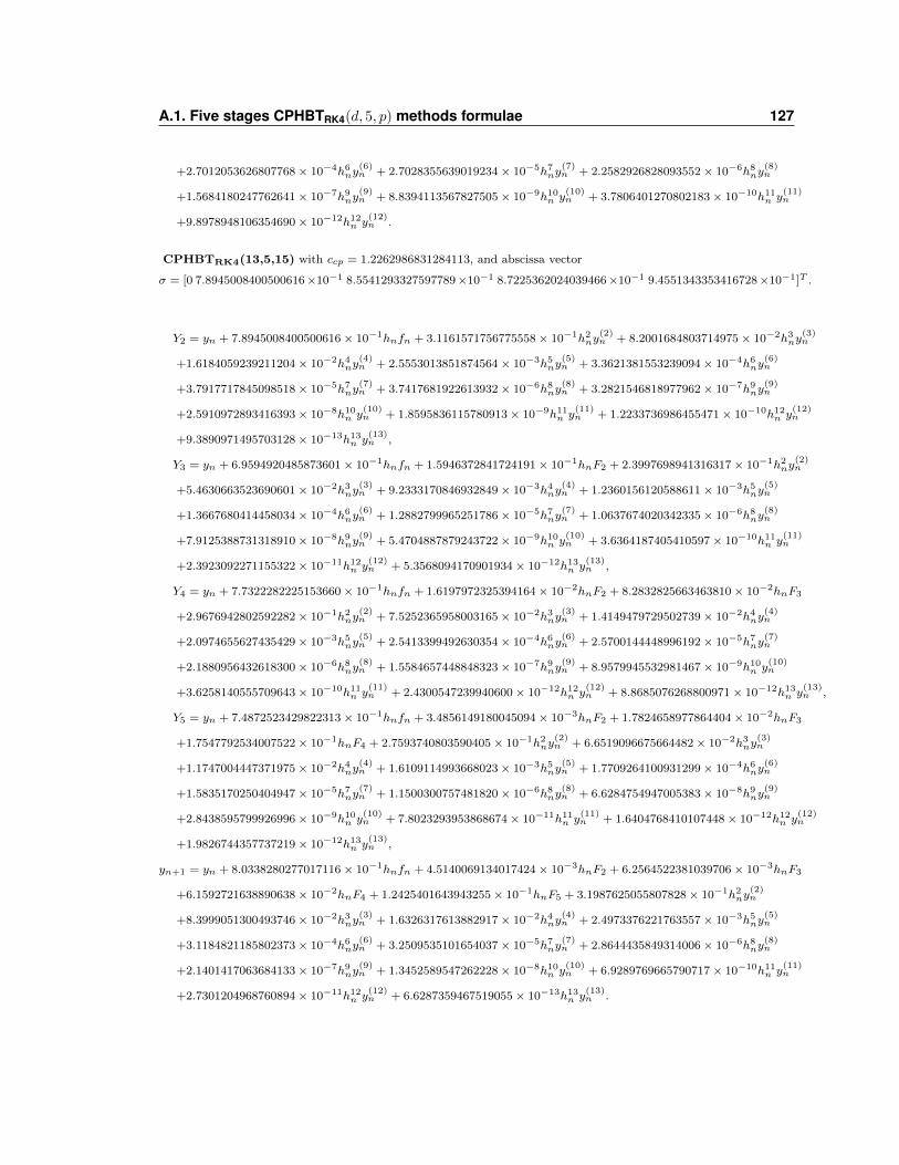
A.1. Five stages CPHBTRK4(d, 5, p) methods formulae 127
+2.7012053626807768× 10⁻⁴h6ny(6)n + 2.7028355639019234× 10⁻⁵h7ny
(7)n + 2.2582926828093552× 10⁻⁶h8ny
(8)n
+1.5684180247762641× 10⁻⁷h9ny(9)n + 8.8394113567827505× 10⁻⁹h10n y
(10)n + 3.7806401270802183× 10⁻¹⁰h11n y
(11)n
+9.8978948106354690× 10⁻¹²h12n y(12)n .
CPHBTRK4(13,5,15) with ccp = 1.2262986831284113, and abscissa vector
σ = [0 7.8945008400500616×10⁻¹ 8.5541293327597789×10⁻¹ 8.7225362024039466×10⁻¹ 9.4551343353416728×10⁻¹]T .
Y2 = yn + 7.8945008400500616× 10⁻¹hnfn + 3.1161571756775558× 10⁻¹h2ny(2)n + 8.2001684803714975× 10⁻²h3ny
(3)n
+1.6184059239211204× 10⁻²h4ny(4)n + 2.5553013851874564× 10⁻³h5ny
(5)n + 3.3621381553239094× 10⁻⁴h6ny
(6)n
+3.7917717845098518× 10⁻⁵h7ny(7)n + 3.7417681922613932× 10⁻⁶h8ny
(8)n + 3.2821546818977962× 10⁻⁷h9ny
(9)n
+2.5910972893416393× 10⁻⁸h10n y(10)n + 1.8595836115780913× 10⁻⁹h11n y
(11)n + 1.2233736986455471× 10⁻¹⁰h12n y
(12)n
+9.3890971495703128× 10⁻¹³h13n y(13)n ,
Y3 = yn + 6.9594920485873601× 10⁻¹hnfn + 1.5946372841724191× 10⁻¹hnF2 + 2.3997698941316317× 10⁻¹h2ny(2)n
+5.4630663523690601× 10⁻²h3ny(3)n + 9.2333170846932849× 10⁻³h4ny
(4)n + 1.2360156120588611× 10⁻³h5ny
(5)n
+1.3667680414458034× 10⁻⁴h6ny(6)n + 1.2882799965251786× 10⁻⁵h7ny
(7)n + 1.0637674020342335× 10⁻⁶h8ny
(8)n
+7.9125388731318910× 10⁻⁸h9ny(9)n + 5.4704887879243722× 10⁻⁹h10n y
(10)n + 3.6364187405410597× 10⁻¹⁰h11n y
(11)n
+2.3923092271155322× 10⁻¹¹h12n y(12)n + 5.3568094170901934× 10⁻¹²h13n y
(13)n ,
Y4 = yn + 7.7322282225153660× 10⁻¹hnfn + 1.6197972325394164× 10⁻²hnF2 + 8.2832825663463810× 10⁻²hnF3
+2.9676942802592282× 10⁻¹h2ny(2)n + 7.5252365958003165× 10⁻²h3ny
(3)n + 1.4149479729502739× 10⁻²h4ny
(4)n
+2.0974655627435429× 10⁻³h5ny(5)n + 2.5413399492630354× 10⁻⁴h6ny
(6)n + 2.5700144448996192× 10⁻⁵h7ny
(7)n
+2.1880956432618300× 10⁻⁶h8ny(8)n + 1.5584657448848323× 10⁻⁷h9ny
(9)n + 8.9579945532981467× 10⁻⁹h10n y
(10)n
+3.6258140555709643× 10⁻¹⁰h11n y(11)n + 2.4300547239940600× 10⁻¹²h12n y
(12)n + 8.8685076268800971× 10⁻¹²h13n y
(13)n ,
Y5 = yn + 7.4872523429822313× 10⁻¹hnfn + 3.4856149180045094× 10⁻³hnF2 + 1.7824658977864404× 10⁻²hnF3
+1.7547792534007522× 10⁻¹hnF4 + 2.7593740803590405× 10⁻¹h2ny(2)n + 6.6519096675664482× 10⁻²h3ny
(3)n
+1.1747004447371975× 10⁻²h4ny(4)n + 1.6109114993668023× 10⁻³h5ny
(5)n + 1.7709264100931299× 10⁻⁴h6ny
(6)n
+1.5835170250404947× 10⁻⁵h7ny(7)n + 1.1500300757481820× 10⁻⁶h8ny
(8)n + 6.6284754947005383× 10⁻⁸h9ny
(9)n
+2.8438595799926996× 10⁻⁹h10n y(10)n + 7.8023293953868674× 10⁻¹¹h11n y
(11)n + 1.6404768410107448× 10⁻¹²h12n y
(12)n
+1.9826744357737219× 10⁻¹²h13n y(13)n ,
yn+1 = yn + 8.0338280277017116× 10⁻¹hnfn + 4.5140069134017424× 10⁻³hnF2 + 6.2564522381039706× 10⁻³hnF3
+6.1592721638890638× 10⁻²hnF4 + 1.2425401643943255× 10⁻¹hnF5 + 3.1987625055807828× 10⁻¹h2ny(2)n
+8.3999051300493746× 10⁻²h3ny(3)n + 1.6326317613882917× 10⁻²h4ny
(4)n + 2.4973376221763557× 10⁻³h5ny
(5)n
+3.1184821185802373× 10⁻⁴h6ny(6)n + 3.2509535101654037× 10⁻⁵h7ny
(7)n + 2.8644435849314006× 10⁻⁶h8ny
(8)n
+2.1401417063684133× 10⁻⁷h9ny(9)n + 1.3452589547262228× 10⁻⁸h10n y
(10)n + 6.9289769665790717× 10⁻¹⁰h11n y
(11)n
+2.7301204968760894× 10⁻¹¹h12n y(12)n + 6.6287359467519055× 10⁻¹³h13n y
(13)n .
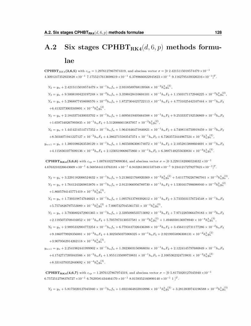
A.2. Six stages CPHBTRK4(d, 6, p) methods formulae 128
A.2 Six stages CPHBTRK4(d, 6, p) methods formu-
lae
CPHBTRK4(2,6,5) with ccp = 1.2976127867974319, and abscissa vector σ = [0 2.4215115018574479×10⁻¹
4.3091247352923828×10⁻¹ 7.1755217613698619×10⁻¹ 6.3789666822945823×10⁻¹ 9.1162795439326216×10⁻¹]T .
Y2 = yn + 2.4215115018574479× 10⁻¹hnfn + 2.9318589768139568× 10⁻²h2ny(2)n ,
Y3 = yn + 9.5008189423197248× 10⁻²hnfn + 3.3590428410604101× 10⁻¹hnF2 + 1.1503171172946225× 10⁻²h2ny(2)n ,
Y4 = yn + 5.2968877458690576× 10⁻²hnfn + 1.8727304425722113× 10⁻¹hnF2 + 4.7731025442107444× 10⁻¹hnF3
+6.4132373003349891× 10⁻³h2ny(2)n ,
Y5 = yn + 2.1843373430033702× 10⁻¹hnfn + 1.6095619405664588× 10⁻¹hnF2 + 9.2533337192536869× 10⁻²hnF3
+1.6597340267993835× 10⁻¹hnF4 + 5.5120066613837957× 10⁻³h2ny(2)n ,
Y6 = yn + 1.4414214514717352× 10⁻¹hnfn + 1.9641646471846821× 10⁻¹hnF2 + 4.7408116750919459× 10⁻²hnF3
+8.5034071941227127× 10⁻²hnF4 + 4.3862715583547374× 10⁻¹hnF5 + 6.7263572444967524× 10⁻³h2ny(2)n ,
yn+1 = yn + 1.3801086263538129× 10⁻¹hnfn + 1.8655696308174072× 10⁻¹hnF2 + 2.1052813888604691× 10⁻¹hnF3
+4.1158361077699136× 10⁻²hnF4 + 2.1230519068675860× 10⁻¹hnF5 + 6.3887148255630834× 10⁻³h2ny(2)n .
CPHBTRK4(3,6,6) with ccp = 1.0078102279098364, and abscissa vector σ = [0 3.2291182006524632×10⁻¹
4.6763210226643609×10⁻¹ 6.5685844113763181×10⁻¹ 6.9432613831537349×10⁻¹ 9.2341217279277621×10⁻¹]T .
Y2 = yn + 3.2291182006524632× 10⁻¹hnfn + 5.2136021768920369× 10⁻²h2ny(2)n + 5.6117792267867941× 10⁻³h3ny
(3)n ,
Y3 = yn + 1.7641243269853876× 10⁻¹hnfn + 2.9121966956789730× 10⁻¹hnF2 + 1.5301617996088940× 10⁻²h2ny(2)n
+1.8605794145771419× 10⁻³h3ny(3)n ,
Y4 = yn + 1.7393198747646021× 10⁻¹hnfn + 1.0957613789392612× 10⁻¹hnF2 + 3.7335031576724548× 10⁻¹hnF3
+5.7574826797553089× 10⁻³h2ny(2)n + 7.0007327045361735× 10⁻⁴h3ny
(3)n ,
Y5 = yn + 3.7936802472901365× 10⁻¹hnfn + 2.3395090535713092× 10⁻²hnF2 + 7.9712285966478183× 10⁻²hnF3
+2.1185073708416852× 10⁻¹hnF4 + 5.7057873130557581× 10⁻²h2ny(2)n + 1.4946938136978940× 10⁻⁴h3ny
(3)n ,
Y6 = yn + 2.9895332904772254× 10⁻¹hnfn + 6.7783447326436388× 10⁻²hnF2 + 3.4564112731177286× 10⁻²hnF3
+9.1860779928356881× 10⁻²hnF4 + 4.3025050375908325× 10⁻¹hnF5 + 2.9219955896308131× 10⁻²h2ny(2)n
+3.9079562914262118× 10⁻⁴h3ny(3)n ,
yn+1 = yn + 2.2541962441999902× 10⁻¹hnfn + 1.3923603156968034× 10⁻¹hnF2 + 2.1224145797680849× 10⁻¹hnF3
+4.1742717395043566× 10⁻²hnF4 + 1.9551135099759831× 10⁻¹hnF5 + 2.1005362324719831× 10⁻²h2ny(2)n
+8.3314370352840692× 10⁻⁴h3ny(3)n .
CPHBTRK4(4,6,7) with ccp = 1.2976127867974319, and abscissa vector σ = [0 5.8175020127045940×10⁻¹
6.7572512798376727×10⁻¹ 6.7629581434464170×10⁻¹ 8.0159352160890140×10⁻¹ 1 ]T .
Y2 = yn + 5.8175020127045940× 10⁻¹hnfn + 1.6921664833910996× 10⁻¹h2ny(2)n + 3.2813939743196588× 10⁻²h3ny
(3)n
A.2. Six stages CPHBTRK4(d, 6, p) methods formulae 129
+4.7723790125203357× 10⁻³h4ny(4)n ,
Y3 = yn + 4.5301985728846905× 10⁻¹hnfn + 2.2270527069529814× 10⁻¹hnF2 + 9.8743388243357461× 10⁻²h2ny(2)n
+1.3737743768911162× 10⁻²h3ny(3)n + 1.3791469365360038× 10⁻³h4ny
(4)n ,
Y4 = yn + 4.9709212539320363× 10⁻¹hnfn + 4.0176733493457517× 10⁻²hnF2 + 1.3902695545798058× 10⁻¹hnF3
+1.1137118418379514× 10⁻¹h2ny(2)n + 1.3014846925126651× 10⁻²h3ny
(3)n + 2.4880245871400700× 10⁻⁴h4ny
(4)n ,
Y5 = yn + 4.6430377340366097× 10⁻¹hnfn + 1.4266679898329707× 10⁻²hnF2 + 4.9368201401443879× 10⁻²hnF3
+2.7365486690546686× 10⁻¹hnF4 + 9.4545467766839364× 10⁻²h2ny(2)n + 9.5776585998835016× 10⁻³h3ny
(3)n
+8.8349269035725003× 10⁻⁵h4ny(4)n ,
Y6 = yn + 4.4620004854413337× 10⁻¹hnfn + 7.1311781552299914× 10⁻³hnF2 + 2.4676620061979952× 10⁻²hnF3
+1.3678596722254405× 10⁻¹hnF4 + 3.8520618601611267× 10⁻¹hnF5 + 7.7890263135432028× 10⁻²h2ny(2)n
+4.7873780215476032× 10⁻³h3ny(3)n + 4.4161247176497030× 10⁻⁵h4ny
(4)n ,
yn+1 = yn + 4.4397514115499548× 10⁻¹hnfn + 7.5590360796050110× 10⁻²hnF2 + 3.8064580818115215× 10⁻²hnF3
+2.1099731207317030× 10⁻¹hnF4 + 1.5687520953351156× 10⁻¹hnF5 + 8.7359952367507501× 10⁻²h2ny(2)n
+9.2837831189798437× 10⁻³h3ny(3)n + 4.6810842957626948× 10⁻⁴h4ny
(4)n .
CPHBTRK4(5,6,8) with ccp = 1.1225568710407938, and abscissa vector σ = [0 5.9208218739488050×10⁻¹
7.1901190437089968×10⁻¹ 7.0621996522392172×10⁻¹ 8.2709525423172647×10⁻¹ 9.9491542708620018×10⁻¹]T .
Y2 = yn + 5.9208218739488050× 10⁻¹hnfn + 1.7528065831515316× 10⁻¹h2ny(2)n + 3.4593518527750174× 10⁻²h3ny
(3)n
+5.1205515298989122× 10⁻³h4ny(4)n + 6.0635747009814994× 10⁻⁴h5ny
(5)n ,
Y3 = yn + 4.4296705227179839× 10⁻¹hnfn + 2.7604485209910123× 10⁻¹hnF2 + 9.5047819463601760× 10⁻²h2ny(2)n
+1.3566913531582599× 10⁻²h3ny(3)n + 1.5867362585522914× 10⁻³h4ny
(4)n + 1.8789565495598578× 10⁻⁴h5ny
(5)n ,
Y4 = yn + 5.5795991165715542× 10⁻¹hnfn + 3.5073730263139015× 10⁻²hnF2 + 1.1318632330362730× 10⁻¹hnF3
+1.4722447483885984× 10⁻¹h2ny(2)n + 2.3298966273411572× 10⁻²h3ny
(3)n + 2.1390391016160716× 10⁻³h4ny
(4)n
+2.3873662085468692× 10⁻⁵h5ny(5)n ,
Y5 = yn + 5.1377386222119970× 10⁻¹hnfn + 1.0576002609036548× 10⁻²hnF2 + 3.4129784359564028× 10⁻²hnF3
+2.6861560504192616× 10⁻¹hnF4 + 1.2153999252821983× 10⁻¹h2ny(2)n + 1.6639281461178327× 10⁻²h3ny
(3)n
+1.2498087514679335× 10⁻³h4ny(4)n + 7.1987755676071587× 10⁻⁶h5ny
(5)n ,
Y6 = yn + 5.1995897059784735× 10⁻¹hnfn + 4.1715419032875940× 10⁻³hnF2 + 1.3461969599408076× 10⁻²hnF3
+1.0595130256039248× 10⁻¹hnF4 + 3.5137164242526475× 10⁻¹hnF5 + 1.1733639834272332× 10⁻¹h2ny(2)n
+1.3320585234133830× 10⁻²h3ny(3)n + 4.9296787931861323× 10⁻⁴h4ny
(4)n + 2.8394465321876344× 10⁻⁶h5ny
(5)n ,
yn+1 = yn + 4.9097666002944390× 10⁻¹hnfn + 7.4072713392728778× 10⁻²hnF2 + 2.5025183291748233× 10⁻²hnF3
+1.9695860601929985× 10⁻¹hnF4 + 1.4587115075975474× 10⁻¹hnF5 + 1.1164949111933453× 10⁻¹h2ny(2)n
+1.4996390713219837× 10⁻²h3ny(3)n + 1.2229106818657672× 10⁻³h4ny
(4)n + 5.0419128961382324× 10⁻⁵h5ny
(5)n .
A.2. Six stages CPHBTRK4(d, 6, p) methods formulae 130
CPHBTRK4(6,6,9) with ccp = 1.0677538948928231, and abscissa vector σ = [0 8.0726307132940789×10⁻¹
6.2830676593582724×10⁻¹ 7.5250397719891582×10⁻¹ 8.5338851860941456×10⁻¹ 9.6977571275092012×10⁻¹ ]T .
Y2 = yn + 8.0726307132940789× 10⁻¹hnfn + 3.2583683316609435× 10⁻¹h2ny(2)n + 8.7678680897969749× 10⁻²h3ny
(3)n
+1.7694940307951539× 10⁻²h4ny(4)n + 2.8568943719974992× 10⁻³h5ny
(5)n + 3.8437755420040018× 10⁻⁴h6ny
(6)n ,
Y3 = yn + 6.0215464503282234× 10⁻¹hnfn + 2.6152120903004880× 10⁻²hnF2 + 1.7627305461843149× 10⁻¹h2ny(2)n
+3.2818055753360324× 10⁻²h3ny(3)n + 4.2004695763476979× 10⁻³h4ny
(4)n + 3.5321587753450615× 10⁻⁴h5ny
(5)n
+1.0733369952717966× 10⁻⁵h6ny(6)n ,
Y4 = yn + 4.7185216983821010× 10⁻¹hnfn + 7.6240354091905898× 10⁻³hnF2 + 2.7302777195151523× 10⁻¹hnF3
+1.0543131920422481× 10⁻¹h2ny(2)n + 1.4643402080623579× 10⁻²h3ny
(3)n + 1.4052741303366180× 10⁻³h4ny
(4)n
+1.0297177683596529× 10⁻⁴h5ny(5)n + 7.6204106310126564× 10⁻⁶h6ny
(6)n ,
Y5 = yn + 5.4758871848532087× 10⁻¹hnfn + 1.9154073700206448× 10⁻³hnF2 + 6.8593517546604393× 10⁻²hnF3
+2.3529087520746864× 10⁻¹hnF4 + 1.4243465364471233× 10⁻¹h2ny(2)n + 2.2801565971915409× 10⁻²h3ny
(3)n
+2.3854694120173945× 10⁻³h4ny(4)n + 1.4892084080236166× 10⁻⁴h5ny
(5)n + 1.9144967070365330× 10⁻⁶h6ny
(6)n ,
Y6 = yn + 6.1703688111968735× 10⁻¹hnfn + 5.4384124236589372× 10⁻⁴hnF2 + 1.9475744107839574× 10⁻²hnF3
+6.6806092475674789× 10⁻²hnF4 + 2.6591315380535258× 10⁻¹hnF5 + 1.8035761908078810× 10⁻¹h2ny(2)n
+3.2241826798008771× 10⁻²h3ny(3)n + 3.7116650428930804× 10⁻³h4ny
(4)n + 2.4273425769940520× 10⁻⁴h5ny
(5)n
+5.4358267800177604× 10⁻⁷h6ny(6)n ,
yn+1 = yn + 5.3005588964943273× 10⁻¹hnfn + 2.1860901690953570× 10⁻³hnF2 + 7.8287061394509277× 10⁻²hnF3
+2.6854186593390089× 10⁻¹hnF4 + 2.6742407320733554× 10⁻²hnF5 + 1.3280651415556025× 10⁻¹h2ny(2)n
+2.0441621260746994× 10⁻²h3ny(3)n + 2.0799858047412328× 10⁻³h4ny
(4)n + 1.3637746665177018× 10⁻⁴h5ny
(5)n
+4.6867084951139577× 10⁻⁶h6ny(6)n .
CPHBTRK4(7,6,10) with ccp = 1.0372974566873341, and abscissa vector σ = [0 8.2577571013225815×10⁻¹
6.6492858252664744×10⁻¹ 7.7518460288634661×10⁻¹ 8.6833765675039798×10⁻¹ 9.7245357209238958×10⁻¹]T .
Y2 = yn + 8.2577571013225815× 10⁻¹hnfn + 3.4095276172221639× 10⁻¹h2ny(2)n + 9.3850169644238646× 10⁻²h3ny
(3)n
+1.9374797621000809× 10⁻²h4ny(4)n + 3.1998474528301011× 10⁻³h5ny
(5)n + 4.4039271711260439× 10⁻⁴h6ny
(6)n
+5.1952229815818279× 10⁻⁵h7ny(7)n ,
Y3 = yn + 6.4186009478336448× 10⁻¹hnfn + 2.3068487743282944× 10⁻²hnF2 + 2.0201561308255761× 10⁻¹h2ny(2)n
+4.1132216628267090× 10⁻²h3ny(3)n + 5.9799749477806637× 10⁻³h4ny
(4)n + 6.3621558608725737× 10⁻⁴h5ny
(5)n
+4.6222016613351427× 10⁻⁵h6ny(6)n + 1.2431588634386864× 10⁻⁶h7ny
(7)n ,
Y4 = yn + 5.1966918829608832× 10⁻¹hnfn + 5.9713118050173956× 10⁻³hnF2 + 2.4954410278524083× 10⁻¹hnF3
+1.2959561348694473× 10⁻¹h2ny(2)n + 2.0434776116002699× 10⁻²h3ny
(3)n + 2.2581519014919457× 10⁻³h4ny
(4)n
+1.8440360636623072× 10⁻⁴h5ny(5)n + 1.1964636630130731× 10⁻⁵h6ny
(6)n + 7.8937035355585419× 10⁻⁷h7ny
(7)n ,
Y5 = yn + 5.9025551353408701× 10⁻¹hnfn + 1.3615701504434488× 10⁻³hnF2 + 5.6900696641896030× 10⁻²hnF3
+2.1981987642397149× 10⁻¹hnF4 + 1.6764490833238621× 10⁻¹h2ny(2)n + 3.0033493926366672× 10⁻²h3ny
(3)n
A.2. Six stages CPHBTRK4(d, 6, p) methods formulae 131
+3.7070628800189459× 10⁻³h4ny(4)n + 3.1682343145137337× 10⁻⁴h5ny
(5)n + 1.6640646719525480× 10⁻⁵h6ny
(6)n
+1.7999112190777956× 10⁻⁷h7ny(7)n ,
Y6 = yn + 6.5959195228523460× 10⁻¹hnfn + 3.4294678829149643× 10⁻⁴hnF2 + 1.4331917572174004× 10⁻²hnF3
+5.5367342327302151× 10⁻²hnF4 + 2.4281941311938737× 10⁻¹hnF5 + 2.0925092469737130× 10⁻¹h2ny(2)n
+4.1804562901158367× 10⁻²h3ny(3)n + 5.7318318926584504× 10⁻³h4ny
(4)n + 5.3856577059708036× 10⁻⁴h5ny
(5)n
+2.9849091421330360× 10⁻⁵h6ny(6)n + 4.5335436561352374× 10⁻⁸h7ny
(7)n ,
yn+1 = yn + 5.7301509266165696× 10⁻¹hnfn + 1.5669421778113602× 10⁻³hnF2 + 6.5483296241495959× 10⁻²hnF3
+2.5297634189316814× 10⁻¹hnF4 + 2.1519888656418292× 10⁻²hnF5 + 1.5728953245544339× 10⁻¹h2ny(2)n
+2.7136973568336459× 10⁻²h3ny(3)n + 3.2275735374709693× 10⁻³h4ny
(4)n + 2.7006268212665887× 10⁻⁴h5ny
(5)n
+1.5135902842873110× 10⁻⁵h6ny(6)n + 4.5646672801272238× 10⁻⁷h7ny
(7)n .
CPHBTRK4(8,6,11) with ccp= 6.5356080481107670×10⁻¹, and abscissa vector σ = [0 6.5087863532715440×10⁻¹
7.0654875715362375×10⁻¹ 9.1376178971858601×10⁻¹ 8.3344995221094431×10⁻¹ 9.4535874251759922×10⁻¹]T .
Y2 = yn + 6.5087863532715440× 10⁻¹hnfn + 2.1182149896266930× 10⁻¹h2ny(2)n + 4.5956696059258097× 10⁻²h3ny
(3)n
+7.4780579037986702× 10⁻³h4ny(4)n + 9.7346162466438175× 10⁻⁴h5ny
(5)n + 1.0560089563415098× 10⁻⁴h6ny
(6)n
+9.8190524056687467× 10⁻⁶h7ny(7)n +−3.8116902287253406× 10⁻¹⁵h8ny
(8)n ,
Y3 = yn + 5.5085339965904634× 10⁻¹hnfn + 1.5569535749457744× 10⁻¹hnF2 + 1.4826679130482112× 10⁻¹h2ny(2)n
+2.5806545148937987× 10⁻²h3ny(3)n + 3.2285794663505047× 10⁻³h4ny
(4)n + 3.0303664563469384× 10⁻⁴h5ny
(5)n
+2.1227228536452358× 10⁻⁵h6ny(6)n + 9.9915125481966478× 10⁻⁷h7ny
(7)n + 1.1559045373283776× 10⁻⁸h8ny
(8)n ,
Y4 = yn + 4.2735262500270949× 10⁻¹hnfn + 4.4923939710489399× 10⁻²hnF2 + 4.4148522500538717× 10⁻¹hnF3
+7.6309434573329699× 10⁻²h2ny(2)n + 7.4461544457900507× 10⁻³h3ny
(3)n + 1.0305197693432373× 10⁻³h4ny
(4)n
+3.8839689249606062× 10⁻⁴h5ny(5)n + 1.1693420065543834× 10⁻⁴h6ny
(6)n + 2.4507406128613122× 10⁻⁵h7ny
(7)n
+3.9134087348729651× 10⁻⁶h8ny(8)n ,
Y5 = yn + 7.6634878604078260× 10⁻¹hnfn + 1.4948999079956653× 10⁻³hnF2 + 1.4690969369559067× 10⁻²hnF3
+5.0915296892607043× 10⁻²hnF4 + 2.8944207404606009× 10⁻¹h2ny(2)n + 7.1251382214370801× 10⁻²h3ny
(3)n
+1.2698454883163554× 10⁻²h4ny(4)n + 1.7085935086651174× 10⁻³h5ny
(5)n + 1.7222370110735698× 10⁻⁴h6ny
(6)n
+1.1567646237306843× 10⁻⁵h7ny(7)n + 1.3022353203800895× 10⁻⁷h8ny
(8)n ,
Y6 = yn + 6.6681279687701434× 10⁻¹hnfn + 2.6070833006391805× 10⁻⁴hnF2 + 2.5620833013539905× 10⁻³hnF3
+8.8795523746943023× 10⁻³hnF4 + 2.6684360163447274× 10⁻¹hnF5 + 2.1435706707299398× 10⁻¹h2ny(2)n
+4.3729946547701411× 10⁻²h3ny(3)n + 6.2396386988725150× 10⁻³h4ny
(4)n + 6.4077743813611347× 10⁻⁴h5ny
(5)n
+4.5965559989036774× 10⁻⁵h6ny(6)n + 2.0173803685982059× 10⁻⁶h7ny
(7)n + 4.6822093160349545× 10⁻⁸h8ny
(8)n ,
yn+1 = yn + 5.3151195913554916× 10⁻¹hnfn + 2.8854850608260395× 10⁻²hnF2 + 2.7877293318834395× 10⁻¹hnF3
+7.9098735495526445× 10⁻⁴hnF4 + 2.3770332752933908× 10⁻²hnF5 + 1.3486677637220160× 10⁻¹h2ny(2)n
+2.1479796786362360× 10⁻²h3ny(3)n + 2.3659105517097076× 10⁻³h4ny
(4)n + 1.8599838398004252× 10⁻⁴h5ny
(5)n
+1.0266109091019705× 10⁻⁵h6ny(6)n + 3.6473009496940092× 10⁻⁷h7ny
(7)n + 6.2751677741251466× 10⁻⁹h8ny
(8)n .
A.2. Six stages CPHBTRK4(d, 6, p) methods formulae 132
CPHBTRK4(9, 6, 12) with ccp= 9.9163130315966042×10⁻¹, and abscissa vector σ = [0 8.5568256645013996×10⁻¹
7.1829693393055971×10⁻¹ 8.0835544845753426×10⁻¹ 8.8980234528386681×10⁻¹ 9.7567281938112871×10⁻¹]T .
Y2 = yn + 8.5568256645013996× 10⁻¹hnfn + 3.6609632726334906× 10⁻¹h2ny(2)n + 1.0442074829355763× 10⁻¹h3ny
(3)n
+2.2337753472618866× 10⁻²h4ny(4)n + 3.8228052440362082× 10⁻³h5ny
(5)n + 5.4518463370932600× 10⁻⁴h6ny
(6)n
+6.6643569508796518× 10⁻⁵h7ny(7)n + 7.1282175743356624× 10⁻⁶h8ny
(8)n + 6.7772127869139232× 10⁻⁷h9ny
(9)n ,
Y3 = yn + 7.0032387510619154× 10⁻¹hnfn + 1.7973058824368105× 10⁻²hnF2 + 2.4259600954522675× 10⁻¹h2ny(2)n
+5.5187737782493251× 10⁻²h3ny(3)n + 9.2151107182336153× 10⁻³h4ny
(4)n + 1.1919736246642830× 10⁻³h5ny
(5)n
+1.2205437013104496× 10⁻⁴h6ny(6)n + 9.7761743593585443× 10⁻⁶h7ny
(7)n + 5.5977694224758458× 10⁻⁷h8ny
(8)n
+1.2156801810285854× 10⁻⁸h9ny(9)n ,
Y4 = yn + 5.9253804964276735× 10⁻¹hnfn + 3.7790846964182783× 10⁻³hnF2 + 2.1203831411834850× 10⁻¹hnF3
+1.7117909772661233× 10⁻¹h2ny(2)n + 3.1950954904935901× 10⁻²h3ny
(3)n + 4.2991986294050764× 10⁻³h4ny
(4)n
+4.3995842070519627× 10⁻⁴h5ny(5)n + 3.5189487487470358× 10⁻⁵h6ny
(6)n + 2.2401550747435463× 10⁻⁶h7ny
(7)n
+1.1920417110245276× 10⁻⁷h8ny(8)n + 6.5142505217891534× 10⁻⁹h9ny
(9)n ,
Y5 = yn + 6.5225547192463695× 10⁻¹hnfn + 7.3327692956782933× 10⁻⁴hnF2 + 4.1142711343481492× 10⁻²hnF3
+1.9567088508618058× 10⁻¹hnF4 + 2.0752234507578865× 10⁻¹h2ny(2)n + 4.2604870773856586× 10⁻²h3ny
(3)n
+6.2756226953662323× 10⁻³h4ny(4)n + 6.9432484726877225× 10⁻⁴h5ny
(5)n + 5.8166925177690642× 10⁻⁵h6ny
(6)n
+3.5517957695381351× 10⁻⁶h7ny(7)n + 1.3567209577595762× 10⁻⁷h8ny
(8)n + 1.2639876550905203× 10⁻⁹h9ny
(9)n ,
Y6 = yn + 7.2075952122256659× 10⁻¹hnfn + 1.5003061651449836× 10⁻⁴hnF2 + 8.4172968211253581× 10⁻³hnF3
+4.0031846060581737× 10⁻²hnF4 + 2.0631412466034044× 10⁻¹hnF5 + 2.5385547529513375× 10⁻¹h2ny(2)n
+5.7816607679521070× 10⁻²h3ny(3)n + 9.4732176422683261× 10⁻³h4ny
(4)n + 1.1701172028993881× 10⁻³h5ny
(5)n
+1.0997733968369118× 10⁻⁴h6ny(6)n + 7.5740152977001563× 10⁻⁶h7ny
(7)n + 3.2206534412851753× 10⁻⁷h8ny
(8)n
+2.5860379801980058× 10⁻¹⁰h9ny(9)n ,
yn+1 = yn + 6.3769782436600186× 10⁻¹hnfn + 8.4507585951567590× 10⁻⁴hnF2 + 4.7415786695281098× 10⁻²hnF3
+2.2550450654635593× 10⁻¹hnF4 + 1.5037770460171211× 10⁻²hnF5 + 1.9783881742796200× 10⁻¹h2ny(2)n
+3.9512215213133563× 10⁻²h3ny(3)n + 5.6542687574121630× 10⁻³h4ny
(4)n + 6.0866317220988314× 10⁻⁴h5ny
(5)n
+5.0062835142051295× 10⁻⁵h6ny(6)n + 3.0966865898048209× 10⁻⁶h7ny
(7)n + 1.3443315671020195× 10⁻⁷h8ny
(8)n
+3.2502867248596942× 10⁻⁹h9ny(9)n .
CPHBTRK4(10,6,13) with ccp= 9.7891787765377547×10⁻¹, and abscissa vector σ = [0 8.7216793659067693×10⁻¹
7.3455764850691607×10⁻¹ 8.1757120453712473×10⁻¹ 8.9651910639916765×10⁻¹ 9.7496976750604369×10⁻¹]T .
Y2 = yn + 8.7216793659067693× 10⁻¹hnfn + 3.8033845480841949× 10⁻¹h2ny(2)n + 1.1057300177878189× 10⁻¹h3ny
(3)n
+2.4109556701009359× 10⁻²h4ny(4)n + 4.2055164640070510× 10⁻³h5ny
(5)n + 6.1131943611852479× 10⁻⁴h6ny
(6)n
+7.6167601599609963× 10⁻⁵h7ny(7)n + 8.3038674902740692× 10⁻⁶h8ny
(8)n + 8.0470744163497083× 10⁻⁷h9ny
(9)n
+7.0184002892993493× 10⁻⁸h10n y(10)n ,
Y3 = yn + 7.2012730214911580× 10⁻¹hnfn + 1.4430346357800395× 10⁻²hnF2 + 2.5720178408283345× 10⁻¹h2ny(2)n
A.2. Six stages CPHBTRK4(d, 6, p) methods formulae 133
+6.0569734092327014× 10⁻²h3ny(3)n + 1.0535273068813885× 10⁻²h4ny
(4)n + 1.4342568517131792× 10⁻³h5ny
(5)n
+1.5749689808795212× 10⁻⁴h6ny(6)n + 1.4073976601458831× 10⁻⁵h7ny
(7)n + 1.0031357604274832× 10⁻⁶h8ny
(8)n
+5.1753607888684203× 10⁻⁸h9ny(9)n + 9.9142792981533817× 10⁻¹⁰h10n y
(10)n ,
Y4 = yn + 6.1666636939405672× 10⁻¹hnfn + 2.7984750143857798× 10⁻³hnF2 + 1.9810636012868230× 10⁻¹hnF3
+1.8625005501485570× 10⁻¹h2ny(2)n + 3.6569540601767869× 10⁻²h3ny
(3)n + 5.2202276081466138× 10⁻³h4ny
(4)n
+5.7333986969055597× 10⁻⁴h5ny(5)n + 4.9955600014877659× 10⁻⁵h6ny
(6)n + 3.5105648832820824× 10⁻⁶h7ny
(7)n
+2.0199739121807016× 10⁻⁷h8ny(8)n + 1.0036569808495538× 10⁻⁸h9ny
(9)n + 5.2663391534795842× 10⁻¹⁰h10n y
(10)n ,
Y5 = yn + 6.6879859693051713× 10⁻¹hnfn + 5.2130954680464753× 10⁻⁴hnF2 + 3.6903933852158038× 10⁻²hnF3
+1.9029526606968783× 10⁻¹hnF4 + 2.1873058782821597× 10⁻¹h2ny(2)n + 4.6342355201246521× 10⁻²h3ny
(3)n
+7.0893782334120270× 10⁻³h4ny(4)n + 8.2350328604301074× 10⁻⁴h5ny
(5)n + 7.3925833067888403× 10⁻⁵h6ny
(6)n
+5.0587192636392605× 10⁻⁶h7ny(7)n + 2.4688209624789656× 10⁻⁷h8ny
(8)n + 6.9903818955404693× 10⁻⁹h9ny
(9)n
+9.8103176312352046× 10⁻¹¹h10n y(10)n ,
Y6 = yn + 7.4176380457262048× 10⁻¹hnfn + 9.7315866934121088× 10⁻⁵hnF2 + 6.8890706838519791× 10⁻³hnF3
+3.5523517465872519× 10⁻²hnF4 + 1.9069605891676469× 10⁻¹hnF5 + 2.7013206313673471× 10⁻¹h2ny(2)n
+6.4058587138924733× 10⁻²h3ny(3)n + 1.1045878291482814× 10⁻²h4ny
(4)n + 1.4611266868308343× 10⁻³h5ny
(5)n
+1.5174660155378573× 10⁻⁴h6ny(6)n + 1.2335402746447030× 10⁻⁵h7ny
(7)n + 7.5037597758261154× 10⁻⁷h8ny
(8)n
+2.8660479124037351× 10⁻⁸h9ny(9)n + 1.8313487083344824× 10⁻¹¹h10n y
(10)n ,
yn+1 = yn + 6.5942861217613780× 10⁻¹hnfn + 5.8392170607958266× 10⁻⁴hnF2 + 4.1336300376774014× 10⁻²hnF3
+2.1315077980703817× 10⁻¹hnF4 + 1.3450052318548556× 10⁻²hnF5 + 2.1255576091346373× 10⁻¹h2ny(2)n
+4.4405639039154392× 10⁻²h3ny(3)n + 6.7132711449553002× 10⁻³h4ny
(4)n + 7.7509361264270515× 10⁻⁴h5ny
(5)n
+7.0071732288657962× 10⁻⁵h6ny(6)n + 4.9751023352591012× 10⁻⁶h7ny
(7)n + 2.7100069746079071× 10⁻⁷h8ny
(8)n
+1.0517882730774634× 10⁻⁸h9ny(9)n + 2.3004926750783143× 10⁻¹⁰h10n y
(10)n .
Appendix B
CPHBTRK5(p− 4, s, p) formulae
B.1 Eight stages CPHBTRK5(p−4, 8, p) methods for-
mulae
CPHBTRK5(2,8,6) with ccp = 1.7887086633648770, and abscissa vector σ = [0 2.7374840363797043×10⁻¹
4.5658640304921172×10⁻¹ 4.1283532228170239×10⁻¹ 4.8070171447096005×10⁻¹ 7.3916285851534802×10⁻¹
8.6532176997823984×10⁻¹ 9.1643089653967069×10⁻¹]T
Y2 = yn + 2.7374840363797043× 10⁻¹hnfn + 3.7469094247168593× 10⁻²h2ny(2)n
Y3 = yn + 1.5070365407323477× 10⁻¹hnfn + 3.0588274897597695× 10⁻¹hnF2 + 2.0500657492140875× 10⁻²h2ny(2)n
Y4 = yn + 2.0780487165097125× 10⁻¹hnfn + 7.2507797907122584× 10⁻²hnF2 + 1.3252265272360861× 10⁻¹hnF3
+4.8595664037269087× 10⁻³h2ny(2)n
Y5 = yn + 2.0134651993002337× 10⁻¹hnfn + 2.6509116516975090× 10⁻²hnF2 + 4.8450767277317522× 10⁻²hnF3
+2.0439531074664413× 10⁻¹hnF4 + 1.7766752782009357× 10⁻³h2ny(2)n
Y6 = yn + 1.4313900660529966× 10⁻¹hnfn + 1.8845099736681054× 10⁻²hnF2 + 3.4443227901431346× 10⁻²hnF3
+1.4530284380710670× 10⁻¹hnF4 + 3.9743268046482932× 10⁻¹hnF5 + 1.2630229602692438× 10⁻³h2ny(2)n
Y7 = yn + 1.9083046103368298× 10⁻¹hnfn + 1.3521350617302660× 10⁻¹hnF2 + 1.6347321865646934× 10⁻²hnF3
+6.8963108460088407× 10⁻²hnF4 + 1.8862805482612396× 10⁻¹hnF5 + 2.6533931761967083× 10⁻¹hnF6
+1.4639231496678199× 10⁻²h2ny(2)n
Y8 = yn + 1.7812861593143697× 10⁻¹hnfn + 1.5786156799529541× 10⁻¹hnF2 + 1.7935856764543159× 10⁻¹hnF3
+3.5742513219759790× 10⁻²hnF4 + 9.7762985479441469× 10⁻²hnF5 + 8.6121364308031828× 10⁻²hnF6
+1.8145528196027358× 10⁻¹hnF7 + 1.2390232299531368× 10⁻²h2ny(2)n
yn+1 = yn + 1.8075533857622461× 10⁻¹hnfn + 9.5820862600417209× 10⁻²hnF2 + 1.1893847441760788× 10⁻¹hnF3
134
B.1. Eight stages CPHBTRK5(p− 4, 8, p) methods formulae 135
+1.0826361778870985× 10⁻¹hnF4 + 1.4395480408615213× 10⁻¹hnF5 + 1.4141603745982614× 10⁻¹hnF6
+5.1666554932071694× 10⁻²hnF7 + 1.5918431013899040× 10⁻¹hnF8 + 1.0450037630755806× 10⁻²h2ny(2)n
CPHBTRK5(3,8,7) with ccp = 1.4301700462580107, and abscissa vector σ = [0 4.1901165948273023×10⁻¹
4.4757325832024575×10⁻¹ 4.5277129402054028×10⁻¹ 6.0594401398694331×10⁻¹ 7.5615644157974560×10⁻¹
8.9787029959899645×10⁻¹ 9.0803080383130441×10⁻¹]T
Y2 = yn + 4.1901165948273023× 10⁻¹hnfn + 8.7785385391235732× 10⁻²h2ny(2)n + 1.2261033337037569× 10⁻²h3ny
(3)n
Y3 = yn + 3.0569128968756548× 10⁻¹hnfn + 1.4188196863268027× 10⁻¹hnF2 + 4.0710711654244683× 10⁻²h2ny(2)n
+2.4879517684760167× 10⁻³h3ny(3)n
Y4 = yn + 2.9965216785588289× 10⁻¹hnfn + 2.5829099290801412× 10⁻²hnF2 + 1.2729002687385593× 10⁻¹hnF3
+3.4706616508130984× 10⁻²h2ny(2)n + 4.5292262207792885× 10⁻⁴h3ny
(3)n
Y5 = yn + 2.4325155235107554× 10⁻¹hnfn + 1.0990984940026231× 10⁻²hnF2 + 5.4165371879008183× 10⁻²hnF3
+2.9753610481683335× 10⁻¹hnF4 + 2.0019944028470162× 10⁻²h2ny(2)n + 1.9273090641787306× 10⁻⁴h3ny
(3)n
Y6 = yn + 2.9365213309221716× 10⁻¹hnfn + 4.7870137955370318× 10⁻³hnF2 + 2.3591187126543709× 10⁻²hnF3
+1.2958888090560947× 10⁻¹hnF4 + 3.0453722665983812× 10⁻¹hnF5 + 3.0115048157946720× 10⁻²h2ny(2)n
+8.3942022747099970× 10⁻⁵h3ny(3)n
Y7 = yn + 3.7473634586941112× 10⁻¹hnfn + 4.6547631248905569× 10⁻²hnF2 + 9.7181246971988992× 10⁻³hnF3
+5.3382684697295089× 10⁻²hnF4 + 1.2545069172417800× 10⁻¹hnF5 + 2.8803482136200770× 10⁻¹hnF6
+6.1246335999288588× 10⁻²h2ny(2)n + 4.7322051061649837× 10⁻³h3ny
(3)n
Y8 = yn + 2.8695124981194142× 10⁻¹hnfn + 6.1487913773827806× 10⁻²hnF2 + 2.1504415616235822× 10⁻²hnF3
+1.1812602474343520× 10⁻¹hnF4 + 2.7759921777488938× 10⁻¹hnF5 + 4.1534676597778750× 10⁻²hnF6
+1.0082730551319606× 10⁻¹hnF7 + 3.3240802553153995× 10⁻²h2ny(2)n + 1.6428972860892126× 10⁻³h3ny
(3)n
yn+1 = yn + 2.7682104631993659× 10⁻¹hnfn + 3.5675932299269984× 10⁻²hnF2 + 9.5468361801232846× 10⁻²hnF3
+1.1437308074564843× 10⁻¹hnF4 + 2.3746250685919018× 10⁻¹hnF5 + 1.1857151878401898× 10⁻²hnF6
+2.8777262045268905× 10⁻²hnF7 + 1.9956465805105117× 10⁻¹hnF8 + 3.0633482765549919× 10⁻²h2ny(2)n
+1.3929472061346105× 10⁻³h3ny(3)n
CPHBTRK5(4,8,8) with ccp = 1.2659158342655910, and abscissa vector σ = [0 4.6549546831062921×10⁻¹
5.1034026450176229×10⁻¹ 5.1168465455700396×10⁻¹ 6.4457785369866316×10⁻¹ 7.7055098081628315×10⁻¹
9.0748644687260571×10⁻¹ 9.2028905345425827×10⁻¹]T
Y2 = yn + 4.6549546831062921× 10⁻¹hnfn + 1.0834301550886601× 10⁻¹h2ny(2)n + 1.6811060914161780× 10⁻²h3ny
(3)n
+1.9563681682590629× 10⁻³h4ny(4)n
Y3 = yn + 3.6380282758188648× 10⁻¹hnfn + 1.4653743691987589× 10⁻¹hnF2 + 6.2011079961807464× 10⁻²h2ny(2)n
+6.2764731280630180× 10⁻³h3ny(3)n + 3.6291424141126434× 10⁻⁴h4ny
(4)n
Y4 = yn + 3.8008660937586147× 10⁻¹hnfn + 2.0592060949110085× 10⁻²hnF2 + 1.1100598423203252× 10⁻¹hnF3
+6.4674258445319321× 10⁻²h2ny(2)n + 5.6417097613508565× 10⁻³h3ny
(3)n + 5.0998245469019597× 10⁻⁵h4ny
(4)n
B.1. Eight stages CPHBTRK5(p− 4, 8, p) methods formulae 136
Y5 = yn + 3.2115506150902295× 10⁻¹hnfn + 7.2269700862404749× 10⁻³hnF2 + 3.8958554436157630× 10⁻²hnF3
+2.7723726766724216× 10⁻¹hnF4 + 4.2636008402430772× 10⁻²h2ny(2)n + 2.4853235196206987× 10⁻³h3ny
(3)n
+1.7898295627819029× 10⁻⁵h4ny(4)n
Y6 = yn + 3.8530610883393435× 10⁻¹hnfn + 2.5006658695534340× 10⁻³hnF2 + 1.3480383372227078× 10⁻²hnF3
+9.5929243455099109× 10⁻²hnF4 + 2.7333457928546917× 10⁻¹hnF5 + 6.3559837715972345× 10⁻²h2ny(2)n
+4.8851319371224404× 10⁻³h3ny(3)n + 6.1931428791837387× 10⁻⁶h4ny
(4)n
Y7 = yn + 4.7060010974195571× 10⁻¹hnfn + 7.0904412156906488× 10⁻³hnF2 + 4.9406394610072499× 10⁻³hnF3
+3.5158629546919035× 10⁻²hnF4 + 1.0017861057183432× 10⁻¹hnF5 + 2.8951801633519869× 10⁻¹hnF6
+1.0029241367077595× 10⁻¹h2ny(2)n + 1.1781452863415523× 10⁻²h3ny
(3)n + 6.9695929781549127× 10⁻⁴h4ny
(4)n
Y8 = yn + 3.6025096680073893× 10⁻¹hnfn + 4.5922132089482856× 10⁻²hnF2 + 1.3662872530663393× 10⁻²hnF3
+9.7227874686875840× 10⁻²hnF4 + 2.7703480179345696× 10⁻¹hnF5 + 3.3845068498470743× 10⁻²hnF6
+9.2345337054569654× 10⁻²hnF7 + 5.6914710641376057× 10⁻²h2ny(2)n + 4.7972871137271361× 10⁻³h3ny
(3)n
+1.9315336079997545× 10⁻⁴h4ny(4)n
yn+1 = yn + 3.4837195819006461× 10⁻¹hnfn + 2.4099023203914976× 10⁻²hnF2 + 7.6677095876881346× 10⁻²hnF3
+1.0917946698940810× 10⁻¹hnF4 + 2.3315884398441686× 10⁻¹hnF5 + 7.7032074763077095× 10⁻³hnF6
+2.1017989395798298× 10⁻²hnF7 + 1.7979241488320813× 10⁻¹hnF8 + 5.3025873534678025× 10⁻²h2ny(2)n
+4.2639564123841071× 10⁻³h3ny(3)n + 1.5707173962518938× 10⁻⁴h4ny
(4)n
CPHBTRK5(5,8,9) with ccp = 1.1275980963815175, and abscissa vector σ = [0 5.2916638242436365×10⁻¹
5.4717079927184487×10⁻¹ 5.5332133691141594×10⁻¹ 6.6326676999053613×10⁻¹ 7.8739643637687862×10⁻¹
9.0889684717619790×10⁻¹ 9.3096254350452368×10⁻¹]T
Y2 = yn + 5.2916638242436365× 10⁻¹hnfn + 1.4000853014404391× 10⁻¹h2ny(2)n + 2.4695935801625393× 10⁻²h3ny
(3)n
+3.2670647521826084× 10⁻³h4ny(4)n + 3.4576416721172421× 10⁻⁴h5ny
(5)n
Y3 = yn + 4.3540355099259298× 10⁻¹hnfn + 1.1176724827925191× 10⁻¹hnF2 + 9.0554471342437354× 10⁻²h2ny(2)n
+1.1655079335988349× 10⁻²h3ny(3)n + 9.7471550769325714× 10⁻⁴h4ny
(4)n + 4.3576151932388834× 10⁻⁵h5ny
(5)n
Y4 = yn + 4.3732579965100798× 10⁻¹hnfn + 1.2982573102755517× 10⁻²hnF2 + 1.0301296415765253× 10⁻¹hnF3
+8.9846623763868719× 10⁻²h2ny(2)n + 1.0996058893167219× 10⁻²h3ny
(3)n + 7.7247007639110593× 10⁻⁴h4ny
(4)n
+5.0616847664132701× 10⁻⁶h5ny(5)n
Y5 = yn + 3.8792222679216631× 10⁻¹hnfn + 3.5645703301504829× 10⁻³hnF2 + 2.8283835011049294× 10⁻²hnF3
+2.4349613785716995× 10⁻¹hnF4 + 6.7867456158971939× 10⁻²h2ny(2)n + 6.6229909856647569× 10⁻³h3ny
(3)n
+3.2855397504491643× 10⁻⁴h4ny(4)n + 1.3897654337183664× 10⁻⁶h5ny
(5)n
Y6 = yn + 4.3083455174960550× 10⁻¹hnfn + 1.0936206691822964× 10⁻³hnF2 + 8.6775638315206328× 10⁻³hnF3
+7.4705331796727642× 10⁻²hnF4 + 2.7208536832984259× 10⁻¹hnF5 + 8.2868519700826371× 10⁻²h2ny(2)n
+8.6269295556025069× 10⁻³h3ny(3)n + 4.1131347750743502× 10⁻⁴h4ny
(4)n + 4.2638412567534908× 10⁻⁷h5ny
(5)n
Y7 = yn + 5.2935554175905541× 10⁻¹hnfn + 3.3382123178179248× 10⁻⁴hnF2 + 2.6487749625921583× 10⁻³hnF3
+2.2803360053260068× 10⁻²hnF4 + 8.3052447128292697× 10⁻²hnF5 + 2.7070290204121572× 10⁻¹hnF6
B.1. Eight stages CPHBTRK5(p− 4, 8, p) methods formulae 137
+1.3056674571497795× 10⁻¹h2ny(2)n + 1.9019610970213398× 10⁻²h3ny
(3)n + 1.6459596301799176× 10⁻³h4ny
(4)n
+6.3393707741640448× 10⁻⁵h5ny(5)n
Y8 = yn + 4.1615991632964217× 10⁻¹hnfn + 3.2250212169529668× 10⁻²hnF2 + 8.7569597838020544× 10⁻³hnF3
+7.5388853240494588× 10⁻²hnF4 + 2.7457483165616464× 10⁻¹hnF5 + 2.8959269078241059× 10⁻²hnF6
+9.4872501246649477× 10⁻²hnF7 + 7.8625982598329147× 10⁻²h2ny(2)n + 8.5493668994264475× 10⁻³h3ny
(3)n
+5.5262940489358221× 10⁻⁴h4ny(4)n + 1.9341622037383198× 10⁻⁵h5ny
(5)n
yn+1 = yn + 4.0891568072911599× 10⁻¹hnfn + 1.4798464472168647× 10⁻²hnF2 + 7.3040596973247995× 10⁻²hnF3
+6.5967009037703833× 10⁻²hnF4 + 2.4025939675171498× 10⁻¹hnF5 + 2.0724001835159978× 10⁻²hnF6
+1.7037085411893846× 10⁻²hnF7 + 1.5925776478899478× 10⁻¹hnF8 + 7.6280468399285331× 10⁻²h2ny(2)n
+8.2394175322924122× 10⁻³h3ny(3)n + 5.2577863418829592× 10⁻⁴h4ny
(4)n + 1.6300118228193040× 10⁻⁵h5ny
(5)n
CPHBTRK5(6,8,10) with ccp = 1.0102662158967612, and abscissa vector σ = [0 5.6834582459174177×10⁻¹
5.8872834307651145×10⁻¹ 5.9266716271678299×10⁻¹ 6.9119669892206426×10⁻¹ 8.0301319377855152×10⁻¹
9.1514325426020959×10⁻¹ 9.3812312749673699×10⁻¹]T
Y2 = yn + 5.6834582459174177× 10⁻¹hnfn + 1.6150848816543345× 10⁻¹h2ny(2)n + 3.0597558294982948× 10⁻²h3ny
(3)n
+4.3474986249139929× 10⁻³h4ny(4)n + 4.9417653817764127× 10⁻⁴h5ny
(5)n + 4.6810528680743980× 10⁻⁵h6ny
(6)n
Y3 = yn + 4.8192504380628043× 10⁻¹hnfn + 1.0680329927023102× 10⁻¹hnF2 + 1.1259932177794925× 10⁻¹h2ny(2)n
+1.6759338754692318× 10⁻²h3ny(3)n + 1.7375921636098861× 10⁻³h4ny
(4)n + 1.2505020041908140× 10⁻⁴h5ny
(5)n
+5.0508450441324238× 10⁻⁶h6ny(6)n
Y4 = yn + 4.8972551120061442× 10⁻¹hnfn + 1.0025618163404805× 10⁻²hnF2 + 9.2916033352763772× 10⁻²hnF3
+1.1522686229824411× 10⁻¹h2ny(2)n + 1.6974534376519225× 10⁻²h3ny
(3)n + 1.6740791101138286× 10⁻³h4ny
(4)n
+1.0068007848309577× 10⁻⁴h5ny(5)n + 4.7412246776079993× 10⁻⁷h6ny
(6)n
Y5 = yn + 4.4170144047095189× 10⁻¹hnfn + 2.2889737592531457× 10⁻³hnF2 + 2.1213890125468052× 10⁻²hnF3
+2.2599239456639111× 10⁻¹hnF4 + 9.1148019954699053× 10⁻²h2ny(2)n + 1.1300393810174062× 10⁻²h3ny
(3)n
+8.7775864021303685× 10⁻⁴h4ny(4)n + 3.6777668015721458× 10⁻⁵h5ny
(5)n + 1.0824807704508198× 10⁻⁷h6ny
(6)n
Y6 = yn + 4.8533481192208222× 10⁻¹hnfn + 5.8673275445721412× 10⁻⁴hnF2 + 5.4377574822569302× 10⁻³hnF3
+5.7928641433436297× 10⁻²hnF4 + 2.5372525018631881× 10⁻¹hnF5 + 1.0917380670713579× 10⁻¹h2ny(2)n
+1.4481234883226475× 10⁻²h3ny(3)n + 1.1482193711736190× 10⁻³h4ny
(4)n + 4.1900801523674731× 10⁻⁵h5ny
(5)n
+2.7747234791951545× 10⁻⁸h6ny(6)n
Y7 = yn + 5.7596733708092829× 10⁻¹hnfn + 1.5220123159727727× 10⁻⁴hnF2 + 1.4105798246979706× 10⁻³hnF3
+1.5026961600401012× 10⁻²hnF4 + 6.5817521303050255× 10⁻²hnF5 + 2.5676865321953485× 10⁻¹hnF6
+1.5723918021563499× 10⁻¹h2ny(2)n + 2.6320266248509510× 10⁻²h3ny
(3)n + 2.8685272382114706× 10⁻³h4ny
(4)n
+1.8939605862363163× 10⁻⁴h5ny(5)n + 4.7867983502074729× 10⁻⁶h6ny
(6)n
Y8 = yn + 4.6717806055159911× 10⁻¹hnfn + 2.4846798799337950× 10⁻²hnF2 + 5.7262405846307237× 10⁻³hnF3
+6.1001863115636198× 10⁻²hnF4 + 2.6718584447718841× 10⁻¹hnF5 + 2.3107059611988029× 10⁻²hnF6
+8.9077260356356547× 10⁻²hnF7 + 1.0163922419313526× 10⁻¹h2ny(2)n + 1.3309204816804832× 10⁻²h3ny
(3)n
B.1. Eight stages CPHBTRK5(p− 4, 8, p) methods formulae 138
+1.1229597574844965× 10⁻³h4ny(4)n + 6.0183295758714790× 10⁻⁵h5ny
(5)n + 1.8757825874629922× 10⁻⁶h6ny
(6)n
yn+1 = yn + 4.6009981224021063× 10⁻¹hnfn + 1.0450633390164462× 10⁻²hnF2 + 6.3775666473099110× 10⁻²hnF3
+5.3711089532930169× 10⁻²hnF4 + 2.3525253298364060× 10⁻¹hnF5 + 1.7771279587692007× 10⁻²hnF6
+1.3122298402439624× 10⁻²hnF7 + 1.4581668738982345× 10⁻¹hnF8 + 9.9001948787816429× 10⁻²h2ny(2)n
+1.2907611426296940× 10⁻²h3ny(3)n + 1.0921126938947714× 10⁻³h4ny
(4)n + 5.8019066124036735× 10⁻⁵h5ny
(5)n
+1.5545407629659841× 10⁻⁶h6ny(6)n
CPHBTRK5(7,8,11) with ccp= 9.2129728884463769×10⁻¹, and abscissa vector σ = [0 6.0297956070795589×10⁻¹
6.2246735280161303×10⁻¹ 6.2721585402548885×10⁻¹ 7.1725083296018455×10⁻¹ 8.1750732724067177×10⁻¹
9.2145408226271541×10⁻¹ 9.4359073748436306×10⁻¹]T
Y2 = yn + 6.0297956070795589× 10⁻¹hnfn + 1.8179217531577974× 10⁻¹h2ny(2)n + 3.6538988670684183× 10⁻²h3ny
(3)n
+5.5080658343405310× 10⁻³h4ny(4)n + 6.6425022342823090× 10⁻⁴h5ny
(5)n + 6.6754884653819362× 10⁻⁵h6ny
(6)n
+5.7502615748100375× 10⁻⁶h7ny(7)n
Y3 = yn + 5.2275798880583790× 10⁻¹hnfn + 9.9709363995775083× 10⁻²hnF2 + 1.3361009415128178× 10⁻¹h2ny(2)n
+2.2071066092381960× 10⁻²h3ny(3)n + 2.6121204824921308× 10⁻³h4ny
(4)n + 2.2955069014028275× 10⁻⁴h5ny
(5)n
+1.4559775069042984× 10⁻⁵h6ny(6)n + 5.2823033730031047× 10⁻⁷h7ny
(7)n
Y4 = yn + 5.3257206458381301× 10⁻¹hnfn + 7.9626957446034940× 10⁻³hnF2 + 8.6681093697072331× 10⁻²hnF3
+1.3794237005676432× 10⁻¹h2ny(2)n + 2.2883897347505455× 10⁻²h3ny
(3)n + 2.6731651048587427× 10⁻³h4ny
(4)n
+2.2283291777839195× 10⁻⁴h5ny(5)n + 1.1768232275583431× 10⁻⁵h6ny
(6)n + 4.2183976372388931× 10⁻⁸h7ny
(7)n
Y5 = yn + 4.8712964712512519× 10⁻¹hnfn + 1.5527768419036632× 10⁻³hnF2 + 1.6903370308221921× 10⁻²hnF3
+2.1166503868493372× 10⁻¹hnF4 + 1.1300662181773756× 10⁻¹h2ny(2)n + 1.6306629033030547× 10⁻²h3ny
(3)n
+1.5865847127968832× 10⁻³h4ny(4)n + 1.0267554545023126× 10⁻⁴h5ny
(5)n + 3.6865593355713411× 10⁻⁶h6ny
(6)n
+8.2261464814109908× 10⁻⁹h7ny(7)n
Y6 = yn + 5.3394585248586235× 10⁻¹hnfn + 3.3469548433758759× 10⁻⁴hnF2 + 3.6434609015132064× 10⁻³hnF3
+4.5623640647023067× 10⁻²hnF4 + 2.3395967772193568× 10⁻¹hnF5 + 1.3526572059024625× 10⁻¹h2ny(2)n
+2.1138175452081728× 10⁻²h3ny(3)n + 2.1873690255423948× 10⁻³h4ny
(4)n + 1.4402149254392764× 10⁻⁴h5ny
(5)n
+4.5266625519821800× 10⁻⁶h6ny(6)n + 1.7731162085502080× 10⁻⁹h7ny
(7)n
Y7 = yn + 6.1466569211176680× 10⁻¹hnfn + 7.5004843543933383× 10⁻⁵hnF2 + 8.1649507586870312× 10⁻⁴hnF3
+1.0224201367451179× 10⁻²hnF4 + 5.2430074035513821× 10⁻²hnF5 + 2.4324261482857093× 10⁻¹hnF6
+1.8111442955716084× 10⁻¹h2ny(2)n + 3.3446727742397285× 10⁻²h3ny
(3)n + 4.2090177415037011× 10⁻³h4ny
(4)n
+3.5943014443224030× 10⁻⁴h5ny(5)n + 1.8138491920708396× 10⁻⁵h6ny
(6)n + 2.1848779610322565× 10⁻⁷h7ny
(7)n
Y8 = yn + 5.1224193922056838× 10⁻¹hnfn + 1.9290958904697862× 10⁻²hnF2 + 4.0074074265021246× 10⁻³hnF3
+5.0181001332280040× 10⁻²hnF4 + 2.5732998798355028× 10⁻¹hnF5 + 1.8406002266277335× 10⁻²hnF6
+8.2133440350487003× 10⁻²hnF7 + 1.2428150226233631× 10⁻¹h2ny(2)n + 1.8658301349196486× 10⁻²h3ny
(3)n
+1.8901469202658502× 10⁻³h4ny(4)n + 1.3124087778235076× 10⁻⁴h5ny
(5)n + 6.0432806583916487× 10⁻⁶h6ny
(6)n
+1.7115986230225067× 10⁻⁷h7ny(7)n
B.1. Eight stages CPHBTRK5(p− 4, 8, p) methods formulae 139
yn+1 = yn + 5.0391147935251557× 10⁻¹hnfn + 7.4829467774940222× 10⁻³hnF2 + 5.5784735913450331× 10⁻²hnF3
+4.5189152394032664× 10⁻²hnF4 + 2.3173160626157041× 10⁻¹hnF5 + 1.0381051394452100× 10⁻²hnF6
+1.0236719716589524× 10⁻²hnF7 + 1.3528230818989537× 10⁻¹hnF8 + 1.2064033301795153× 10⁻¹h2ny(2)n
+1.7963252571564069× 10⁻²h3ny(3)n + 1.8186186599538341× 10⁻³h4ny
(4)n + 1.2714116670449867× 10⁻⁴h5ny
(5)n
+5.8000201243385346× 10⁻⁶h6ny(6)n + 1.3695545589541550× 10⁻⁷h7ny
(7)n
CPHBTRK5(8, 8, 12) with ccp= 8.3899828718045832×10⁻¹, and abscissa vector σ = [0 6.3442778287933732×10⁻¹
6.4806091964118251×10⁻¹ 6.5778452073891203×10⁻¹ 7.4053651347951488×10⁻¹ 8.3110284752952135×10⁻¹
9.2735138793776239×10⁻¹ 9.4800556307728689×10⁻¹]T
Y2 = yn + 6.3442778287933732× 10⁻¹hnfn + 2.0124930584459580× 10⁻¹h2ny(2)n + 4.2559383637664192× 10⁻²h3ny
(3)n
+6.7502138504886089× 10⁻³h4ny(4)n + 8.5650464142537658× 10⁻⁴h5ny
(5)n + 9.0565056780893895× 10⁻⁵h6ny
(6)n
+8.2081411685491133× 10⁻⁶h7ny(7)n + 6.5093410039040332× 10⁻⁷h8ny
(8)n
Y3 = yn + 5.5991828761338081× 10⁻¹hnfn + 8.8142632027801662× 10⁻²hnF2 + 1.5407134316854010× 10⁻¹h2ny(2)n
+2.7623779892062172× 10⁻²h3ny(3)n + 3.5981073656161508× 10⁻³h4ny
(4)n + 3.5759061708865212× 10⁻⁴h5ny
(5)n
+2.7392899410268045× 10⁻⁵h6ny(6)n + 1.5426932790737223× 10⁻⁶h7ny
(7)n + 4.8137564385466838× 10⁻⁸h8ny
(8)n
Y4 = yn + 5.6601553493298773× 10⁻¹hnfn + 6.3191453543435779× 10⁻³hnF2 + 8.5449840451580661× 10⁻²hnF3
+1.5695449429876798× 10⁻¹h2ny(2)n + 2.8219624670652730× 10⁻²h3ny
(3)n + 3.6553656460089476× 10⁻³h4ny
(4)n
+3.5555085562573676× 10⁻⁴h5ny(5)n + 2.5694849223444351× 10⁻⁵h6ny
(6)n + 1.2079358620528968× 10⁻⁶h7ny
(7)n
+3.4510912524133941× 10⁻⁹h8ny(8)n
Y5 = yn + 5.2677084285373510× 10⁻¹hnfn + 1.0523109471714857× 10⁻³hnF2 + 1.4229741127800948× 10⁻²hnF3
+1.9848361855080737× 10⁻¹hnF4 + 1.3374835757257769× 10⁻¹h2ny(2)n + 2.1544442788534502× 10⁻²h3ny
(3)n
+2.4253119077743551× 10⁻³h4ny(4)n + 1.9592717340050647× 10⁻⁴h5ny
(5)n + 1.0916080320101515× 10⁻⁵h6ny
(6)n
+3.4266972684998814× 10⁻⁷h7ny(7)n + 5.7470130863604662× 10⁻¹⁰h8ny
(8)n
Y6 = yn + 5.7613702206133321× 10⁻¹hnfn + 1.9087312382352843× 10⁻⁴hnF2 + 2.5810575738702186× 10⁻³hnF3
+3.6001895069534565× 10⁻²hnF4 + 2.1619199970095976× 10⁻¹hnF5 + 1.5979263483339215× 10⁻¹h2ny(2)n
+2.8029909245438807× 10⁻²h3ny(3)n + 3.4138373578088666× 10⁻³h4ny
(4)n + 2.9427596137500677× 10⁻⁴h5ny
(5)n
+1.6920775322864040× 10⁻⁵h6ny(6)n + 4.9033154364877436× 10⁻⁷h7ny
(7)n + 1.0424203448578282× 10⁻¹⁰h8ny
(8)n
Y7 = yn + 6.4862655064719066× 10⁻¹hnfn + 3.6769940695116786× 10⁻⁵hnF2 + 4.9721685285373531× 10⁻⁴hnF3
+6.9354318727585934× 10⁻³hnF4 + 4.1647387796267914× 10⁻²hnF5 + 2.2960803082799633× 10⁻¹hnF6
+2.0341342435066243× 10⁻¹h2ny(2)n + 4.0586746183670148× 10⁻²h3ny
(3)n + 5.6748112511148018× 10⁻³h4ny
(4)n
+5.7092740164794271× 10⁻⁴h5ny(5)n + 3.9719428341979857× 10⁻⁵h6ny
(6)n + 1.5555777745779016× 10⁻⁶h7ny
(7)n
+2.0081263140683207× 10⁻¹¹h8ny(8)n
Y8 = yn + 5.5209241164721989× 10⁻¹hnfn + 1.5031111898254198× 10⁻²hnF2 + 2.9496090303136268× 10⁻³hnF3
+4.1142636987470324× 10⁻²hnF4 + 2.4706224342114499× 10⁻¹hnF5 + 1.4493201023321448× 10⁻²hnF6
+7.5234349069562528× 10⁻²hnF7 + 1.4607397169734107× 10⁻¹h2ny(2)n + 2.4353265219505451× 10⁻²h3ny
(3)n
+2.8196597451252271× 10⁻³h4ny(4)n + 2.3435194720078191× 10⁻⁴h5ny
(5)n + 1.3864058168038072× 10⁻⁵h6ny
(6)n
B.1. Eight stages CPHBTRK5(p− 4, 8, p) methods formulae 140
+5.5819444876399311× 10⁻⁷h7ny(7)n + 1.4291909676730649× 10⁻⁸h8ny
(8)n
yn+1 = yn + 5.4145653542767558× 10⁻¹hnfn + 5.5914233410541501× 10⁻³hnF2 + 4.8662147845363705× 10⁻²hnF3
+3.8278997260764475× 10⁻²hnF4 + 2.2986603756187235× 10⁻¹hnF5 + 1.5395891137679231× 10⁻³hnF6
+7.9920171403241869× 10⁻³hnF7 + 1.2661325230917767× 10⁻¹hnF8 + 1.4079205087886684× 10⁻¹h2ny(2)n
+2.3150059902996928× 10⁻²h3ny(3)n + 2.6587905709737395× 10⁻³h4ny
(4)n + 2.2109640724393226× 10⁻⁴h5ny
(5)n
+1.3203681536550432× 10⁻⁵h6ny(6)n + 5.2841027574064201× 10⁻⁷h7ny
(7)n + 1.1157623293823810× 10⁻⁸h8ny
(8)n
CPHBTRK5(9,8,13) with ccp= 7.3981614589567168×10⁻¹, and abscissa vector σ = [0 6.6316884336031645×10⁻¹
6.6552534456124690×10⁻¹ 6.8255131739962571×10⁻¹ 7.5805741411028338×10⁻¹ 8.4399678029601544×10⁻¹
9.3183807109044126×10⁻¹ 9.5217739155443293×10⁻¹]T
Y2 = yn + 6.6316884336031645× 10⁻¹hnfn + 2.1989645740192998× 10⁻¹h2ny(2)n + 4.8609493104756339× 10⁻²h3ny
(3)n
+8.0590753296531353× 10⁻³h4ny(4)n + 1.0689055329839458× 10⁻³h5ny
(5)n + 1.1814414099506766× 10⁻⁴h6ny
(6)n
+1.1192787619071024× 10⁻⁵h7ny(7)n + 9.2783850241462522× 10⁻⁷h8ny
(8)n + 6.8368176274608356× 10⁻⁸h9ny
(9)n
Y3 = yn + 5.9338241815166537× 10⁻¹hnfn + 7.2142926409581462× 10⁻²hnF2 + 1.7361905106301259× 10⁻¹h2ny(2)n
+3.3265548928368548× 10⁻²h3ny(3)n + 4.6674045755896853× 10⁻³h4ny
(4)n + 5.0662692232004232× 10⁻⁴h5ny
(5)n
+4.3571527678842963× 10⁻⁵h6ny(6)n + 2.9509158674938910× 10⁻⁶h7ny
(7)n + 1.4706424099751308× 10⁻⁷h8ny
(8)n
+3.6489803912536636× 10⁻⁹h9ny(9)n
Y4 = yn + 5.8984518218526627× 10⁻¹hnfn + 4.6972541598545676× 10⁻³hnF2 + 8.8008881054504912× 10⁻²hnF3
+1.7125093694557295× 10⁻¹h2ny(2)n + 3.2473882146496276× 10⁻²h3ny
(3)n + 4.4911981767817204× 10⁻³h4ny
(4)n
+4.7725109633802245× 10⁻⁴h5ny(5)n + 3.9658876073627216× 10⁻⁵h6ny
(6)n + 2.5172192199980150× 10⁻⁶h7ny
(7)n
+1.0591526881452161× 10⁻⁷h8ny(8)n + 2.3758632260515969× 10⁻¹⁰h9ny
(9)n
Y5 = yn + 5.6077185743100488× 10⁻¹hnfn + 6.4158452687660924× 10⁻⁴hnF2 + 1.2020881644968782× 10⁻²hnF3
+1.8462309050743317× 10⁻¹hnF4 + 1.5288510762824156× 10⁻¹h2ny(2)n + 2.6794068830641254× 10⁻²h3ny
(3)n
+3.3530122818893069× 10⁻³h4ny(4)n + 3.1302595652995976× 10⁻⁴h5ny
(5)n + 2.1876053777132641× 10⁻⁵h6ny
(6)n
+1.0876560797805447× 10⁻⁶h7ny(7)n + 3.1298087505204534× 10⁻⁸h8ny
(8)n + 3.2451017460208804× 10⁻¹¹h9ny
(9)n
Y6 = yn + 6.0514823130406725× 10⁻¹hnfn + 9.8931071971960921× 10⁻⁵hnF2 + 1.8535963031667672× 10⁻³hnF3
+2.8468517380923878× 10⁻²hnF4 + 2.0842750423588552× 10⁻¹hnF5 + 1.7743482031882651× 10⁻¹h2ny(2)n
+3.3250583050177897× 10⁻²h3ny(3)n + 4.4051727701609929× 10⁻³h4ny
(4)n + 4.2758191550126715× 10⁻⁴h5ny
(5)n
+2.9947870321764276× 10⁻⁵h6ny(6)n + 1.3611818064025165× 10⁻⁶h7ny
(7)n + 2.4514137781210259× 10⁻⁸h8ny
(8)n
+5.0036629033489305× 10⁻¹²h9ny(9)n
Y7 = yn + 6.8028409245184629× 10⁻¹hnfn + 1.5646617872971343× 10⁻⁵hnF2 + 2.9315878690437289× 10⁻⁴hnF3
+4.5024884901171793× 10⁻³hnF4 + 3.2964218905007205× 10⁻²hnF5 + 2.1377846583869312× 10⁻¹hnF6
+2.2546532755835413× 10⁻¹h2ny(2)n + 4.8126851293900992× 10⁻²h3ny
(3)n + 7.3481188463329350× 10⁻³h4ny
(4)n
+8.3834980190962340× 10⁻⁴h5ny(5)n + 7.1713057626288326× 10⁻⁵h6ny
(6)n + 4.3701054524888691× 10⁻⁶h7ny
(7)n
+1.5387781817848601× 10⁻⁷h8ny(8)n + 7.9114271444266149× 10⁻¹³h9ny
(9)n
Y8 = yn + 5.8398742230001055× 10⁻¹hnfn + 1.1649277211928055× 10⁻²hnF2 + 2.1293072296099053× 10⁻³hnF3
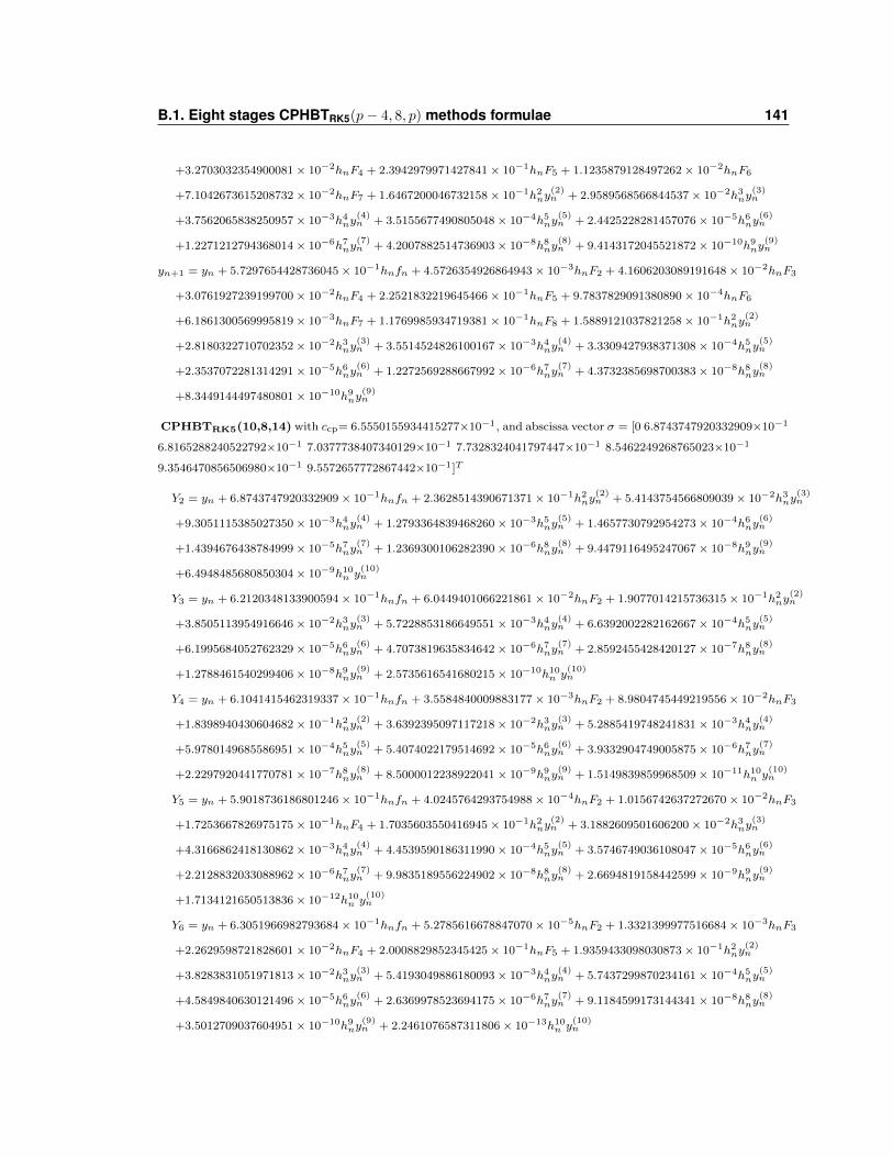
B.1. Eight stages CPHBTRK5(p− 4, 8, p) methods formulae 141
+3.2703032354900081× 10⁻²hnF4 + 2.3942979971427841× 10⁻¹hnF5 + 1.1235879128497262× 10⁻²hnF6
+7.1042673615208732× 10⁻²hnF7 + 1.6467200046732158× 10⁻¹h2ny(2)n + 2.9589568566844537× 10⁻²h3ny
(3)n
+3.7562065838250957× 10⁻³h4ny(4)n + 3.5155677490805048× 10⁻⁴h5ny
(5)n + 2.4425228281457076× 10⁻⁵h6ny
(6)n
+1.2271212794368014× 10⁻⁶h7ny(7)n + 4.2007882514736903× 10⁻⁸h8ny
(8)n + 9.4143172045521872× 10⁻¹⁰h9ny
(9)n
yn+1 = yn + 5.7297654428736045× 10⁻¹hnfn + 4.5726354926864943× 10⁻³hnF2 + 4.1606203089191648× 10⁻²hnF3
+3.0761927239199700× 10⁻²hnF4 + 2.2521832219645466× 10⁻¹hnF5 + 9.7837829091380890× 10⁻⁴hnF6
+6.1861300569995819× 10⁻³hnF7 + 1.1769985934719381× 10⁻¹hnF8 + 1.5889121037821258× 10⁻¹h2ny(2)n
+2.8180322710702352× 10⁻²h3ny(3)n + 3.5514524826100167× 10⁻³h4ny
(4)n + 3.3309427938371308× 10⁻⁴h5ny
(5)n
+2.3537072281314291× 10⁻⁵h6ny(6)n + 1.2272569288667992× 10⁻⁶h7ny
(7)n + 4.3732385698700383× 10⁻⁸h8ny
(8)n
+8.3449144497480801× 10⁻¹⁰h9ny(9)n
CPHBTRK5(10,8,14) with ccp= 6.5550155934415277×10⁻¹, and abscissa vector σ = [0 6.8743747920332909×10⁻¹
6.8165288240522792×10⁻¹ 7.0377738407340129×10⁻¹ 7.7328324041797447×10⁻¹ 8.5462249268765023×10⁻¹
9.3546470856506980×10⁻¹ 9.5572657772867442×10⁻¹]T
Y2 = yn + 6.8743747920332909× 10⁻¹hnfn + 2.3628514390671371× 10⁻¹h2ny(2)n + 5.4143754566809039× 10⁻²h3ny
(3)n
+9.3051115385027350× 10⁻³h4ny(4)n + 1.2793364839468260× 10⁻³h5ny
(5)n + 1.4657730792954273× 10⁻⁴h6ny
(6)n
+1.4394676438784999× 10⁻⁵h7ny(7)n + 1.2369300106282390× 10⁻⁶h8ny
(8)n + 9.4479116495247067× 10⁻⁸h9ny
(9)n
+6.4948485680850304× 10⁻⁹h10n y(10)n
Y3 = yn + 6.2120348133900594× 10⁻¹hnfn + 6.0449401066221861× 10⁻²hnF2 + 1.9077014215736315× 10⁻¹h2ny(2)n
+3.8505113954916646× 10⁻²h3ny(3)n + 5.7228853186649551× 10⁻³h4ny
(4)n + 6.6392002282162667× 10⁻⁴h5ny
(5)n
+6.1995684052762329× 10⁻⁵h6ny(6)n + 4.7073819635834642× 10⁻⁶h7ny
(7)n + 2.8592455428420127× 10⁻⁷h8ny
(8)n
+1.2788461540299406× 10⁻⁸h9ny(9)n + 2.5735616541680215× 10⁻¹⁰h10n y
(10)n
Y4 = yn + 6.1041415462319337× 10⁻¹hnfn + 3.5584840009883177× 10⁻³hnF2 + 8.9804745449219556× 10⁻²hnF3
+1.8398940430604682× 10⁻¹h2ny(2)n + 3.6392395097117218× 10⁻²h3ny
(3)n + 5.2885419748241831× 10⁻³h4ny
(4)n
+5.9780149685586951× 10⁻⁴h5ny(5)n + 5.4074022179514692× 10⁻⁵h6ny
(6)n + 3.9332904749005875× 10⁻⁶h7ny
(7)n
+2.2297920441770781× 10⁻⁷h8ny(8)n + 8.5000012238922041× 10⁻⁹h9ny
(9)n + 1.5149839859968509× 10⁻¹¹h10n y
(10)n
Y5 = yn + 5.9018736186801246× 10⁻¹hnfn + 4.0245764293754988× 10⁻⁴hnF2 + 1.0156742637272670× 10⁻²hnF3
+1.7253667826975175× 10⁻¹hnF4 + 1.7035603550416945× 10⁻¹h2ny(2)n + 3.1882609501606200× 10⁻²h3ny
(3)n
+4.3166862418130862× 10⁻³h4ny(4)n + 4.4539590186311990× 10⁻⁴h5ny
(5)n + 3.5746749036108047× 10⁻⁵h6ny
(6)n
+2.2128832033088962× 10⁻⁶h7ny(7)n + 9.9835189556224902× 10⁻⁸h8ny
(8)n + 2.6694819158442599× 10⁻⁹h9ny
(9)n
+1.7134121650513836× 10⁻¹²h10n y(10)n
Y6 = yn + 6.3051966982793684× 10⁻¹hnfn + 5.2785616678847070× 10⁻⁵hnF2 + 1.3321399977516684× 10⁻³hnF3
+2.2629598721828601× 10⁻²hnF4 + 2.0008829852345425× 10⁻¹hnF5 + 1.9359433098030873× 10⁻¹h2ny(2)n
+3.8283831051971813× 10⁻²h3ny(3)n + 5.4193049886180093× 10⁻³h4ny
(4)n + 5.7437299870234161× 10⁻⁴h5ny
(5)n
+4.5849840630121496× 10⁻⁵h6ny(6)n + 2.6369978523694175× 10⁻⁶h7ny
(7)n + 9.1184599173144341× 10⁻⁸h8ny
(8)n
+3.5012709037604951× 10⁻¹⁰h9ny(9)n + 2.2461076587311806× 10⁻¹³h10n y
(10)n
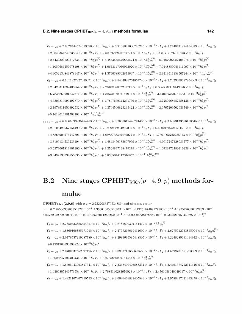
B.2. Nine stages CPHBTRK5(p− 4, 9, p) methods formulae 142
Y7 = yn + 7.0629444574613620× 10⁻¹hnfn + 6.9138847600715215× 10⁻⁶hnF2 + 1.7448431994134819× 10⁻⁴hnF3
+2.9640354243238849× 10⁻³hnF4 + 2.6207658920789721× 10⁻²hnF5 + 1.9981717026911863× 10⁻¹hnF6
+2.4430320723377635× 10⁻¹h2ny(2)n + 5.4853558576865524× 10⁻²h3ny
(3)n + 8.9187902082405075× 10⁻³h4ny
(4)n
+1.1059686459078408× 10⁻³h5ny(5)n + 1.0673147070963020× 10⁻⁴h6ny
(6)n + 7.9448859946511097× 10⁻⁶h7ny
(7)n
+4.3052134849878947× 10⁻⁷h8ny(8)n + 1.3740389362875697× 10⁻⁸h9ny
(9)n + 2.9419511358507244× 10⁻¹⁴h10n y
(10)n
Y8 = yn + 6.1011827827339371× 10⁻¹hnfn + 9.5434083764857746× 10⁻³hnF2 + 1.7323608697954003× 10⁻³hnF3
+2.9428311882405054× 10⁻²hnF4 + 2.2818205362290719× 10⁻¹hnF5 + 8.8853037118449656× 10⁻³hnF6
+6.7836860991842371× 10⁻²hnF7 + 1.8075237232162897× 10⁻¹h2ny(2)n + 3.4400852707815531× 10⁻²h3ny
(3)n
+4.6806819099197870× 10⁻³h4ny(4)n + 4.7807659344261766× 10⁻⁴h5ny
(5)n + 3.7280568657588136× 10⁻⁵h6ny
(6)n
+2.1973911650392532× 10⁻⁶h7ny(7)n + 9.3794560823245422× 10⁻⁸h8ny
(8)n + 2.6767209502936749× 10⁻⁹h9ny
(9)n
+5.1613016981502102× 10⁻¹¹h10n y(10)n
yn+1 = yn + 6.0065699935454753× 10⁻¹hnfn + 3.7680619448774463× 10⁻³hnF2 + 3.5353133566138645× 10⁻²hnF3
+2.5108426567251499× 10⁻²hnF4 + 2.1969938294266037× 10⁻¹hnF5 + 6.4002170259951161× 10⁻⁴hnF6
+4.8863904576247896× 10⁻³hnF7 + 1.0988758346430022× 10⁻¹hnF8 + 1.7561002722285013× 10⁻¹h2ny(2)n
+3.3100134539233494× 10⁻²h3ny(3)n + 4.4848450133697969× 10⁻³h4ny
(4)n + 4.6017247128083777× 10⁻⁴h5ny
(5)n
+3.6572067812901306× 10⁻⁵h6ny(6)n + 2.2504897198419219× 10⁻⁶h7ny
(7)n + 1.0423472480310328× 10⁻⁷h8ny
(8)n
+3.3492133034856635× 10⁻⁹h9ny(9)n + 5.8305044112316857× 10⁻¹¹h10n y
(10)n
B.2 Nine stages CPHBTRK5(p−4, 9, p) methods for-
mulae
CPHBTRK5(2,9,6) with ccp = 2.7322083370534886, and abscissa vector
σ = [0 2.7850633886554327×10⁻¹ 4.3666434505105711×10⁻¹ 4.1325187469127583×10⁻¹ 4.1975726870492769×10⁻¹
6.0472995999901091×10⁻¹ 8.3273650601125326×10⁻¹ 8.7020090463847888×10⁻¹ 9.2342683963440797×10⁻¹]T
Y2 = yn + 2.7850633886554327× 10⁻¹hnfn + 3.8782890394144412× 10⁻²h2ny(2)n
Y3 = yn + 1.8869166885671015× 10⁻¹hnfn + 2.4797267619434699× 10⁻¹hnF2 + 2.6275912933855904× 10⁻²h2ny(2)n
Y4 = yn + 2.0778537219087789× 10⁻¹hnfn + 8.2983695585448505× 10⁻²hnF2 + 1.2248280691494942× 10⁻¹hnF3
+8.7931960633594822× 10⁻³h2ny(2)n
Y5 = yn + 2.0700637552097195× 10⁻¹hnfn + 3.0893713688697588× 10⁻²hnF2 + 4.5598701551223829× 10⁻²hnF3
+1.3625847794403434× 10⁻¹hnF4 + 3.2735886209151453× 10⁻³h2ny(2)n
Y6 = yn + 1.6695043903817541× 10⁻¹hnfn + 2.3368490403888331× 10⁻²hnF2 + 3.4491574252511446× 10⁻²hnF3
+1.0306805346773554× 10⁻¹hnF4 + 2.7685140283670023× 10⁻¹hnF5 + 2.4761938640649917× 10⁻³h2ny(2)n
Y7 = yn + 1.4321707907410533× 10⁻¹hnfn + 2.0046469822405589× 10⁻²hnF2 + 2.9588317021333278× 10⁻²hnF3
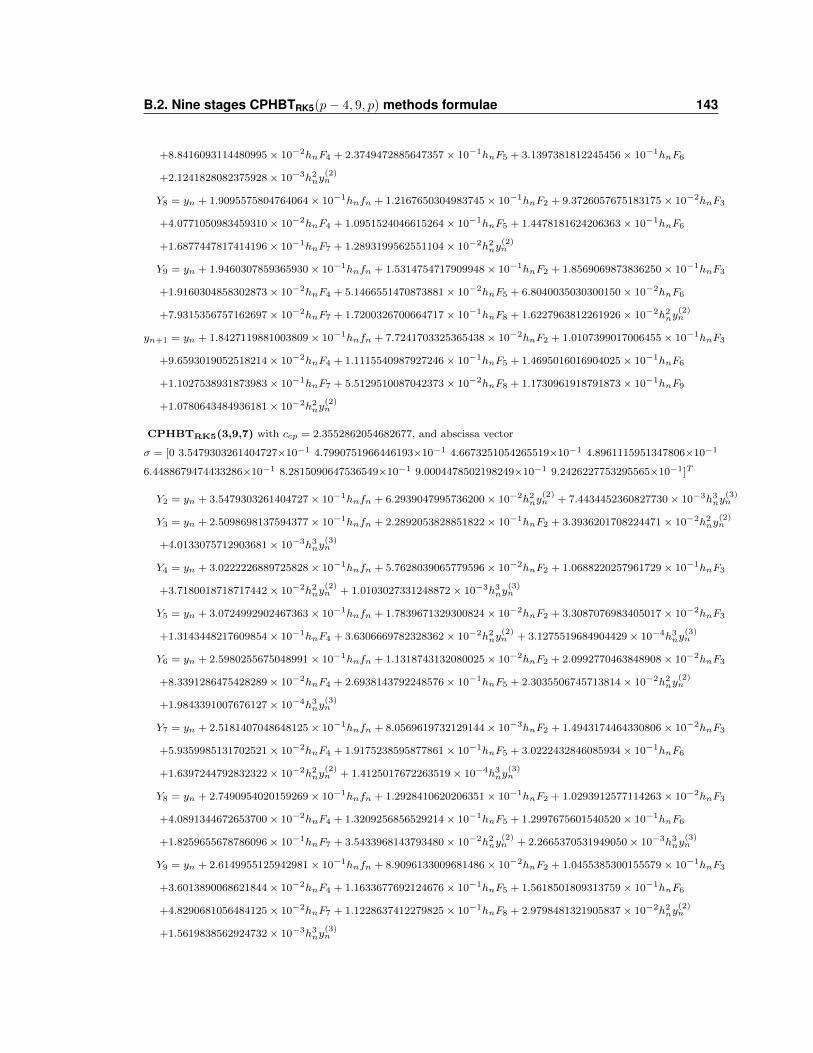
B.2. Nine stages CPHBTRK5(p− 4, 9, p) methods formulae 143
+8.8416093114480995× 10⁻²hnF4 + 2.3749472885647357× 10⁻¹hnF5 + 3.1397381812245456× 10⁻¹hnF6
+2.1241828082375928× 10⁻³h2ny(2)n
Y8 = yn + 1.9095575804764064× 10⁻¹hnfn + 1.2167650304983745× 10⁻¹hnF2 + 9.3726057675183175× 10⁻²hnF3
+4.0771050983459310× 10⁻²hnF4 + 1.0951524046615264× 10⁻¹hnF5 + 1.4478181624206363× 10⁻¹hnF6
+1.6877447817414196× 10⁻¹hnF7 + 1.2893199562551104× 10⁻²h2ny(2)n
Y9 = yn + 1.9460307859365930× 10⁻¹hnfn + 1.5314754717909948× 10⁻¹hnF2 + 1.8569069873836250× 10⁻¹hnF3
+1.9160304858302873× 10⁻²hnF4 + 5.1466551470873881× 10⁻²hnF5 + 6.8040035030300150× 10⁻²hnF6
+7.9315356757162697× 10⁻²hnF7 + 1.7200326700664717× 10⁻¹hnF8 + 1.6227963812261926× 10⁻²h2ny(2)n
yn+1 = yn + 1.8427119881003809× 10⁻¹hnfn + 7.7241703325365438× 10⁻²hnF2 + 1.0107399017006455× 10⁻¹hnF3
+9.6593019052518214× 10⁻²hnF4 + 1.1115540987927246× 10⁻¹hnF5 + 1.4695016016904025× 10⁻¹hnF6
+1.1027538931873983× 10⁻¹hnF7 + 5.5129510087042373× 10⁻²hnF8 + 1.1730961918791873× 10⁻¹hnF9
+1.0780643484936181× 10⁻²h2ny(2)n
CPHBTRK5(3,9,7) with ccp = 2.3552862054682677, and abscissa vector
σ = [0 3.5479303261404727×10⁻¹ 4.7990751966446193×10⁻¹ 4.6673251054265519×10⁻¹ 4.8961115951347806×10⁻¹
6.4488679474433286×10⁻¹ 8.2815090647536549×10⁻¹ 9.0004478502198249×10⁻¹ 9.2426227753295565×10⁻¹]T
Y2 = yn + 3.5479303261404727× 10⁻¹hnfn + 6.2939047995736200× 10⁻²h2ny(2)n + 7.4434452360827730× 10⁻³h3ny
(3)n
Y3 = yn + 2.5098698137594377× 10⁻¹hnfn + 2.2892053828851822× 10⁻¹hnF2 + 3.3936201708224471× 10⁻²h2ny(2)n
+4.0133075712903681× 10⁻³h3ny(3)n
Y4 = yn + 3.0222226889725828× 10⁻¹hnfn + 5.7628039065779596× 10⁻²hnF2 + 1.0688220257961729× 10⁻¹hnF3
+3.7180018718717442× 10⁻²h2ny(2)n + 1.0103027331248872× 10⁻³h3ny
(3)n
Y5 = yn + 3.0724992902467363× 10⁻¹hnfn + 1.7839671329300824× 10⁻²hnF2 + 3.3087076983405017× 10⁻²hnF3
+1.3143448217609854× 10⁻¹hnF4 + 3.6306669782328362× 10⁻²h2ny(2)n + 3.1275519684904429× 10⁻⁴h3ny
(3)n
Y6 = yn + 2.5980255675048991× 10⁻¹hnfn + 1.1318743132080025× 10⁻²hnF2 + 2.0992770463848908× 10⁻²hnF3
+8.3391286475428289× 10⁻²hnF4 + 2.6938143792248576× 10⁻¹hnF5 + 2.3035506745713814× 10⁻²h2ny(2)n
+1.9843391007676127× 10⁻⁴h3ny(3)n
Y7 = yn + 2.5181407048648125× 10⁻¹hnfn + 8.0569619732129144× 10⁻³hnF2 + 1.4943174464330806× 10⁻²hnF3
+5.9359985131702521× 10⁻²hnF4 + 1.9175238595877861× 10⁻¹hnF5 + 3.0222432846085934× 10⁻¹hnF6
+1.6397244792832322× 10⁻²h2ny(2)n + 1.4125017672263519× 10⁻⁴h3ny
(3)n
Y8 = yn + 2.7490954020159269× 10⁻¹hnfn + 1.2928410620206351× 10⁻¹hnF2 + 1.0293912577114263× 10⁻²hnF3
+4.0891344672653700× 10⁻²hnF4 + 1.3209256856529214× 10⁻¹hnF5 + 1.2997675601540520× 10⁻¹hnF6
+1.8259655678786096× 10⁻¹hnF7 + 3.5433968143793480× 10⁻²h2ny(2)n + 2.2665370531949050× 10⁻³h3ny
(3)n
Y9 = yn + 2.6149955125942981× 10⁻¹hnfn + 8.9096133009681486× 10⁻²hnF2 + 1.0455385300155579× 10⁻¹hnF3
+3.6013890068621844× 10⁻²hnF4 + 1.1633677692124676× 10⁻¹hnF5 + 1.5618501809313759× 10⁻¹hnF6
+4.8290681056484125× 10⁻²hnF7 + 1.1228637412279825× 10⁻¹hnF8 + 2.9798481321905837× 10⁻²h2ny(2)n
+1.5619838562924732× 10⁻³h3ny(3)n
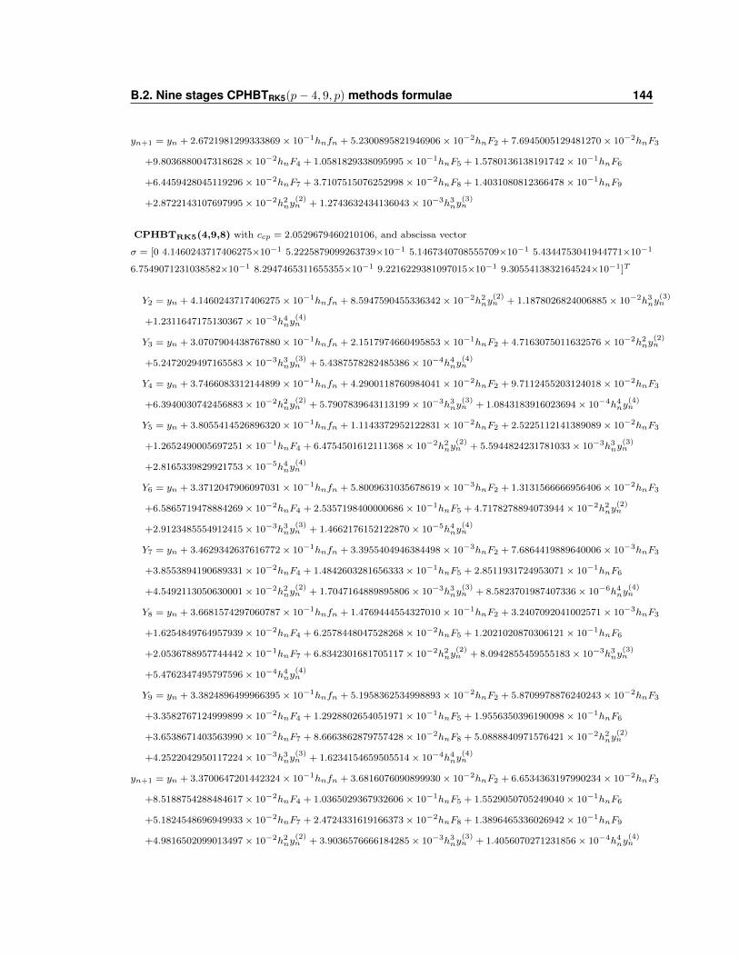
B.2. Nine stages CPHBTRK5(p− 4, 9, p) methods formulae 144
yn+1 = yn + 2.6721981299333869× 10⁻¹hnfn + 5.2300895821946906× 10⁻²hnF2 + 7.6945005129481270× 10⁻²hnF3
+9.8036880047318628× 10⁻²hnF4 + 1.0581829338095995× 10⁻¹hnF5 + 1.5780136138191742× 10⁻¹hnF6
+6.4459428045119296× 10⁻²hnF7 + 3.7107515076252998× 10⁻²hnF8 + 1.4031080812366478× 10⁻¹hnF9
+2.8722143107697995× 10⁻²h2ny(2)n + 1.2743632434136043× 10⁻³h3ny
(3)n
CPHBTRK5(4,9,8) with ccp = 2.0529679460210106, and abscissa vector
σ = [0 4.1460243717406275×10⁻¹ 5.2225879099263739×10⁻¹ 5.1467340708555709×10⁻¹ 5.4344753041944771×10⁻¹
6.7549071231038582×10⁻¹ 8.2947465311655355×10⁻¹ 9.2216229381097015×10⁻¹ 9.3055413832164524×10⁻¹]T
Y2 = yn + 4.1460243717406275× 10⁻¹hnfn + 8.5947590455336342× 10⁻²h2ny(2)n + 1.1878026824006885× 10⁻²h3ny
(3)n
+1.2311647175130367× 10⁻³h4ny(4)n
Y3 = yn + 3.0707904438767880× 10⁻¹hnfn + 2.1517974660495853× 10⁻¹hnF2 + 4.7163075011632576× 10⁻²h2ny(2)n
+5.2472029497165583× 10⁻³h3ny(3)n + 5.4387578282485386× 10⁻⁴h4ny
(4)n
Y4 = yn + 3.7466083312144899× 10⁻¹hnfn + 4.2900118760984041× 10⁻²hnF2 + 9.7112455203124018× 10⁻²hnF3
+6.3940030742456883× 10⁻²h2ny(2)n + 5.7907839643113199× 10⁻³h3ny
(3)n + 1.0843183916023694× 10⁻⁴h4ny
(4)n
Y5 = yn + 3.8055414526896320× 10⁻¹hnfn + 1.1143372952122831× 10⁻²hnF2 + 2.5225112141389089× 10⁻²hnF3
+1.2652490005697251× 10⁻¹hnF4 + 6.4754501612111368× 10⁻²h2ny(2)n + 5.5944824231781033× 10⁻³h3ny
(3)n
+2.8165339829921753× 10⁻⁵h4ny(4)n
Y6 = yn + 3.3712047906097031× 10⁻¹hnfn + 5.8009631035678619× 10⁻³hnF2 + 1.3131566666956406× 10⁻²hnF3
+6.5865719478884269× 10⁻²hnF4 + 2.5357198400000686× 10⁻¹hnF5 + 4.7178278894073944× 10⁻²h2ny(2)n
+2.9123485554912415× 10⁻³h3ny(3)n + 1.4662176152122870× 10⁻⁵h4ny
(4)n
Y7 = yn + 3.4629342637616772× 10⁻¹hnfn + 3.3955404946384498× 10⁻³hnF2 + 7.6864419889640006× 10⁻³hnF3
+3.8553894190689331× 10⁻²hnF4 + 1.4842603281656333× 10⁻¹hnF5 + 2.8511931724953071× 10⁻¹hnF6
+4.5492113050630001× 10⁻²h2ny(2)n + 1.7047164889895806× 10⁻³h3ny
(3)n + 8.5823701987407336× 10⁻⁶h4ny
(4)n
Y8 = yn + 3.6681574297060787× 10⁻¹hnfn + 1.4769444554327010× 10⁻¹hnF2 + 3.2407092041002571× 10⁻³hnF3
+1.6254849764957939× 10⁻²hnF4 + 6.2578448047528268× 10⁻²hnF5 + 1.2021020870306121× 10⁻¹hnF6
+2.0536788957744442× 10⁻¹hnF7 + 6.8342301681705117× 10⁻²h2ny(2)n + 8.0942855459555183× 10⁻³h3ny
(3)n
+5.4762347495797596× 10⁻⁴h4ny(4)n
Y9 = yn + 3.3824896499966395× 10⁻¹hnfn + 5.1958362534998893× 10⁻²hnF2 + 5.8709978876240243× 10⁻²hnF3
+3.3582767124999899× 10⁻²hnF4 + 1.2928802654051971× 10⁻¹hnF5 + 1.9556350396190098× 10⁻¹hnF6
+3.6538671403563990× 10⁻²hnF7 + 8.6663862879757428× 10⁻²hnF8 + 5.0888840971576421× 10⁻²h2ny(2)n
+4.2522042950117224× 10⁻³h3ny(3)n + 1.6234154659505514× 10⁻⁴h4ny
(4)n
yn+1 = yn + 3.3700647201442324× 10⁻¹hnfn + 3.6816076090899930× 10⁻²hnF2 + 6.6534363197990234× 10⁻²hnF3
+8.5188754288484617× 10⁻²hnF4 + 1.0365029367932606× 10⁻¹hnF5 + 1.5529050705249040× 10⁻¹hnF6
+5.1824548696949933× 10⁻²hnF7 + 2.4724331619166373× 10⁻²hnF8 + 1.3896465336026942× 10⁻¹hnF9
+4.9816502099013497× 10⁻²h2ny(2)n + 3.9036576666184285× 10⁻³h3ny
(3)n + 1.4056070271231856× 10⁻⁴h4ny
(4)n
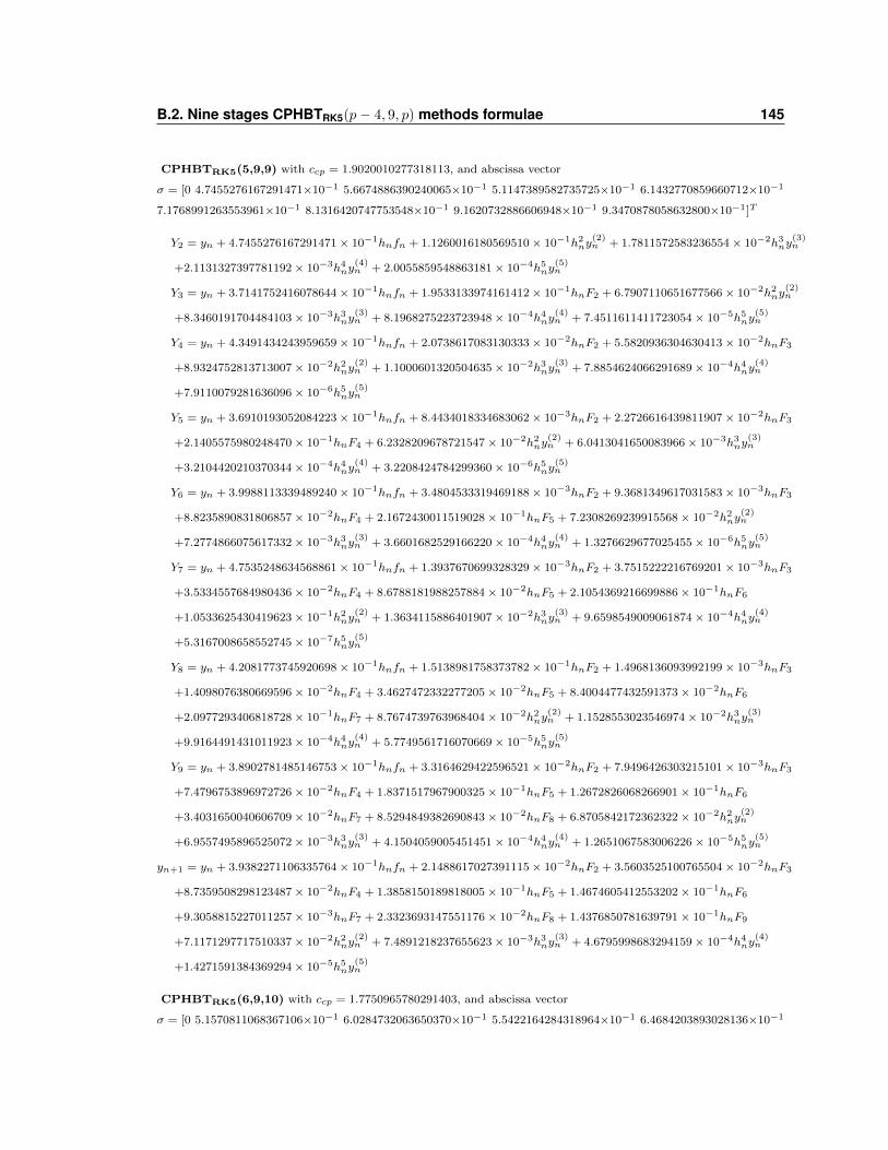
B.2. Nine stages CPHBTRK5(p− 4, 9, p) methods formulae 145
CPHBTRK5(5,9,9) with ccp = 1.9020010277318113, and abscissa vector
σ = [0 4.7455276167291471×10⁻¹ 5.6674886390240065×10⁻¹ 5.1147389582735725×10⁻¹ 6.1432770859660712×10⁻¹
7.1768991263553961×10⁻¹ 8.1316420747753548×10⁻¹ 9.1620732886606948×10⁻¹ 9.3470878058632800×10⁻¹]T
Y2 = yn + 4.7455276167291471× 10⁻¹hnfn + 1.1260016180569510× 10⁻¹h2ny(2)n + 1.7811572583236554× 10⁻²h3ny
(3)n
+2.1131327397781192× 10⁻³h4ny(4)n + 2.0055859548863181× 10⁻⁴h5ny
(5)n
Y3 = yn + 3.7141752416078644× 10⁻¹hnfn + 1.9533133974161412× 10⁻¹hnF2 + 6.7907110651677566× 10⁻²h2ny(2)n
+8.3460191704484103× 10⁻³h3ny(3)n + 8.1968275223723948× 10⁻⁴h4ny
(4)n + 7.4511611411723054× 10⁻⁵h5ny
(5)n
Y4 = yn + 4.3491434243959659× 10⁻¹hnfn + 2.0738617083130333× 10⁻²hnF2 + 5.5820936304630413× 10⁻²hnF3
+8.9324752813713007× 10⁻²h2ny(2)n + 1.1000601320504635× 10⁻²h3ny
(3)n + 7.8854624066291689× 10⁻⁴h4ny
(4)n
+7.9110079281636096× 10⁻⁶h5ny(5)n
Y5 = yn + 3.6910193052084223× 10⁻¹hnfn + 8.4434018334683062× 10⁻³hnF2 + 2.2726616439811907× 10⁻²hnF3
+2.1405575980248470× 10⁻¹hnF4 + 6.2328209678721547× 10⁻²h2ny(2)n + 6.0413041650083966× 10⁻³h3ny
(3)n
+3.2104420210370344× 10⁻⁴h4ny(4)n + 3.2208424784299360× 10⁻⁶h5ny
(5)n
Y6 = yn + 3.9988113339489240× 10⁻¹hnfn + 3.4804533319469188× 10⁻³hnF2 + 9.3681349617031583× 10⁻³hnF3
+8.8235890831806857× 10⁻²hnF4 + 2.1672430011519028× 10⁻¹hnF5 + 7.2308269239915568× 10⁻²h2ny(2)n
+7.2774866075617332× 10⁻³h3ny(3)n + 3.6601682529166220× 10⁻⁴h4ny
(4)n + 1.3276629677025455× 10⁻⁶h5ny
(5)n
Y7 = yn + 4.7535248634568861× 10⁻¹hnfn + 1.3937670699328329× 10⁻³hnF2 + 3.7515222216769201× 10⁻³hnF3
+3.5334557684980436× 10⁻²hnF4 + 8.6788181988257884× 10⁻²hnF5 + 2.1054369216699886× 10⁻¹hnF6
+1.0533625430419623× 10⁻¹h2ny(2)n + 1.3634115886401907× 10⁻²h3ny
(3)n + 9.6598549009061874× 10⁻⁴h4ny
(4)n
+5.3167008658552745× 10⁻⁷h5ny(5)n
Y8 = yn + 4.2081773745920698× 10⁻¹hnfn + 1.5138981758373782× 10⁻¹hnF2 + 1.4968136093992199× 10⁻³hnF3
+1.4098076380669596× 10⁻²hnF4 + 3.4627472332277205× 10⁻²hnF5 + 8.4004477432591373× 10⁻²hnF6
+2.0977293406818728× 10⁻¹hnF7 + 8.7674739763968404× 10⁻²h2ny(2)n + 1.1528553023546974× 10⁻²h3ny
(3)n
+9.9164491431011923× 10⁻⁴h4ny(4)n + 5.7749561716070669× 10⁻⁵h5ny
(5)n
Y9 = yn + 3.8902781485146753× 10⁻¹hnfn + 3.3164629422596521× 10⁻²hnF2 + 7.9496426303215101× 10⁻³hnF3
+7.4796753896972726× 10⁻²hnF4 + 1.8371517967900325× 10⁻¹hnF5 + 1.2672826068266901× 10⁻¹hnF6
+3.4031650040606709× 10⁻²hnF7 + 8.5294849382690843× 10⁻²hnF8 + 6.8705842172362322× 10⁻²h2ny(2)n
+6.9557495896525072× 10⁻³h3ny(3)n + 4.1504059005451451× 10⁻⁴h4ny
(4)n + 1.2651067583006226× 10⁻⁵h5ny
(5)n
yn+1 = yn + 3.9382271106335764× 10⁻¹hnfn + 2.1488617027391115× 10⁻²hnF2 + 3.5603525100765504× 10⁻²hnF3
+8.7359508298123487× 10⁻²hnF4 + 1.3858150189818005× 10⁻¹hnF5 + 1.4674605412553202× 10⁻¹hnF6
+9.3058815227011257× 10⁻³hnF7 + 2.3323693147551176× 10⁻²hnF8 + 1.4376850781639791× 10⁻¹hnF9
+7.1171297717510337× 10⁻²h2ny(2)n + 7.4891218237655623× 10⁻³h3ny
(3)n + 4.6795998683294159× 10⁻⁴h4ny
(4)n
+1.4271591384369294× 10⁻⁵h5ny(5)n
CPHBTRK5(6,9,10) with ccp = 1.7750965780291403, and abscissa vector
σ = [0 5.1570811068367106×10⁻¹ 6.0284732063650370×10⁻¹ 5.5422164284318964×10⁻¹ 6.4684203893028136×10⁻¹
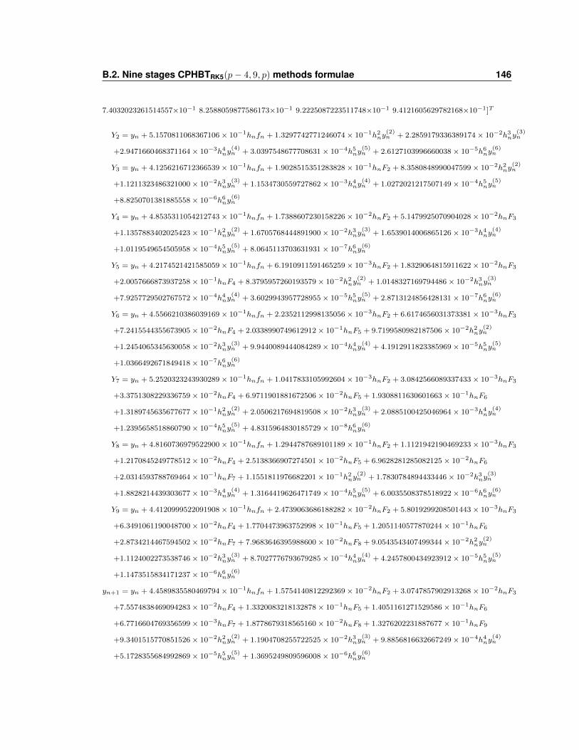
B.2. Nine stages CPHBTRK5(p− 4, 9, p) methods formulae 146
7.4032023261514557×10⁻¹ 8.2588059877586173×10⁻¹ 9.2225087223511748×10⁻¹ 9.4121605629782168×10⁻¹]T
Y2 = yn + 5.1570811068367106× 10⁻¹hnfn + 1.3297742771246074× 10⁻¹h2ny(2)n + 2.2859179336389174× 10⁻²h3ny
(3)n
+2.9471660468371164× 10⁻³h4ny(4)n + 3.0397548677708631× 10⁻⁴h5ny
(5)n + 2.6127103996660038× 10⁻⁵h6ny
(6)n
Y3 = yn + 4.1256216712366539× 10⁻¹hnfn + 1.9028515351283828× 10⁻¹hnF2 + 8.3580848990047599× 10⁻²h2ny(2)n
+1.1211323486321000× 10⁻²h3ny(3)n + 1.1534730559727862× 10⁻³h4ny
(4)n + 1.0272021217507149× 10⁻⁴h5ny
(5)n
+8.8250701381885558× 10⁻⁶h6ny(6)n
Y4 = yn + 4.8535311054212743× 10⁻¹hnfn + 1.7388607230158226× 10⁻²hnF2 + 5.1479925070904028× 10⁻²hnF3
+1.1357883402025423× 10⁻¹h2ny(2)n + 1.6705768444891900× 10⁻²h3ny
(3)n + 1.6539014006865126× 10⁻³h4ny
(4)n
+1.0119549654505958× 10⁻⁴h5ny(5)n + 8.0645113703631931× 10⁻⁷h6ny
(6)n
Y5 = yn + 4.2174521421585059× 10⁻¹hnfn + 6.1910911591465259× 10⁻³hnF2 + 1.8329064815911622× 10⁻²hnF3
+2.0057666873937258× 10⁻¹hnF4 + 8.3795957260193579× 10⁻²h2ny(2)n + 1.0148327169794486× 10⁻²h3ny
(3)n
+7.9257729502767572× 10⁻⁴h4ny(4)n + 3.6029943957728955× 10⁻⁵h5ny
(5)n + 2.8713124856428131× 10⁻⁷h6ny
(6)n
Y6 = yn + 4.5566210386039169× 10⁻¹hnfn + 2.2352112998135056× 10⁻³hnF2 + 6.6174656031373381× 10⁻³hnF3
+7.2415544355673905× 10⁻²hnF4 + 2.0338990749612912× 10⁻¹hnF5 + 9.7199580982187506× 10⁻²h2ny(2)n
+1.2454065345630058× 10⁻²h3ny(3)n + 9.9440089444084289× 10⁻⁴h4ny
(4)n + 4.1912911823385969× 10⁻⁵h5ny
(5)n
+1.0366492671849418× 10⁻⁷h6ny(6)n
Y7 = yn + 5.2520323243930289× 10⁻¹hnfn + 1.0417833105992604× 10⁻³hnF2 + 3.0842566089337433× 10⁻³hnF3
+3.3751308229336759× 10⁻²hnF4 + 6.9711901881672506× 10⁻²hnF5 + 1.9308811630601663× 10⁻¹hnF6
+1.3189745635677677× 10⁻¹h2ny(2)n + 2.0506217694819508× 10⁻²h3ny
(3)n + 2.0885100425046964× 10⁻³h4ny
(4)n
+1.2395658518860790× 10⁻⁴h5ny(5)n + 4.8315964830185729× 10⁻⁸h6ny
(6)n
Y8 = yn + 4.8160736979522900× 10⁻¹hnfn + 1.2944787689101189× 10⁻¹hnF2 + 1.1121942190469233× 10⁻³hnF3
+1.2170845249778512× 10⁻²hnF4 + 2.5138366907274501× 10⁻²hnF5 + 6.9628281285082125× 10⁻²hnF6
+2.0314593788769464× 10⁻¹hnF7 + 1.1551811976682201× 10⁻¹h2ny(2)n + 1.7830784894433446× 10⁻²h3ny
(3)n
+1.8828214439303677× 10⁻³h4ny(4)n + 1.3164419626471749× 10⁻⁴h5ny
(5)n + 6.0035508378518922× 10⁻⁶h6ny
(6)n
Y9 = yn + 4.4120999522091908× 10⁻¹hnfn + 2.4739063686188282× 10⁻²hnF2 + 5.8019299208501443× 10⁻³hnF3
+6.3491061190048700× 10⁻²hnF4 + 1.7704473963752998× 10⁻¹hnF5 + 1.2051140577870244× 10⁻¹hnF6
+2.8734214467594502× 10⁻²hnF7 + 7.9683646395988600× 10⁻²hnF8 + 9.0543543407499344× 10⁻²h2ny(2)n
+1.1124002273538746× 10⁻²h3ny(3)n + 8.7027776793679285× 10⁻⁴h4ny
(4)n + 4.2457800434923912× 10⁻⁵h5ny
(5)n
+1.1473515834171237× 10⁻⁶h6ny(6)n
yn+1 = yn + 4.4589835580469794× 10⁻¹hnfn + 1.5754140812292369× 10⁻²hnF2 + 3.0747857902913268× 10⁻²hnF3
+7.5574838469094283× 10⁻²hnF4 + 1.3320083218132878× 10⁻¹hnF5 + 1.4051161271529586× 10⁻¹hnF6
+6.7716604769356599× 10⁻³hnF7 + 1.8778679318565160× 10⁻²hnF8 + 1.3276202231887677× 10⁻¹hnF9
+9.3401515770851526× 10⁻²h2ny(2)n + 1.1904708255722525× 10⁻²h3ny
(3)n + 9.8856816632667249× 10⁻⁴h4ny
(4)n
+5.1728355684992869× 10⁻⁵h5ny(5)n + 1.3695249809596008× 10⁻⁶h6ny
(6)n
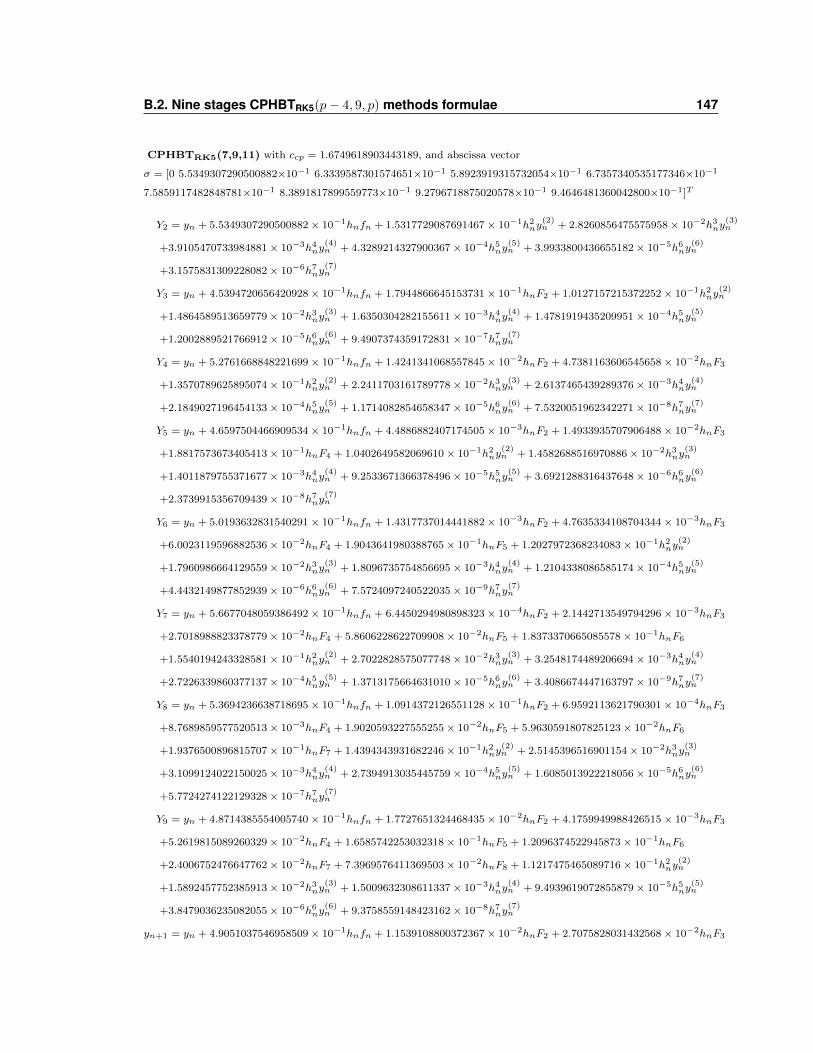
B.2. Nine stages CPHBTRK5(p− 4, 9, p) methods formulae 147
CPHBTRK5(7,9,11) with ccp = 1.6749618903443189, and abscissa vector
σ = [0 5.5349307290500882×10⁻¹ 6.3339587301574651×10⁻¹ 5.8923919315732054×10⁻¹ 6.7357340535177346×10⁻¹
7.5859117482848781×10⁻¹ 8.3891817899559773×10⁻¹ 9.2796718875020578×10⁻¹ 9.4646481360042800×10⁻¹]T
Y2 = yn + 5.5349307290500882× 10⁻¹hnfn + 1.5317729087691467× 10⁻¹h2ny(2)n + 2.8260856475575958× 10⁻²h3ny
(3)n
+3.9105470733984881× 10⁻³h4ny(4)n + 4.3289214327900367× 10⁻⁴h5ny
(5)n + 3.9933800436655182× 10⁻⁵h6ny
(6)n
+3.1575831309228082× 10⁻⁶h7ny(7)n
Y3 = yn + 4.5394720656420928× 10⁻¹hnfn + 1.7944866645153731× 10⁻¹hnF2 + 1.0127157215372252× 10⁻¹h2ny(2)n
+1.4864589513659779× 10⁻²h3ny(3)n + 1.6350304282155611× 10⁻³h4ny
(4)n + 1.4781919435209951× 10⁻⁴h5ny
(5)n
+1.2002889521766912× 10⁻⁵h6ny(6)n + 9.4907374359172831× 10⁻⁷h7ny
(7)n
Y4 = yn + 5.2761668848221699× 10⁻¹hnfn + 1.4241341068557845× 10⁻²hnF2 + 4.7381163606545658× 10⁻²hnF3
+1.3570789625895074× 10⁻¹h2ny(2)n + 2.2411703161789778× 10⁻²h3ny
(3)n + 2.6137465439289376× 10⁻³h4ny
(4)n
+2.1849027196454133× 10⁻⁴h5ny(5)n + 1.1714082854658347× 10⁻⁵h6ny
(6)n + 7.5320051962342271× 10⁻⁸h7ny
(7)n
Y5 = yn + 4.6597504466909534× 10⁻¹hnfn + 4.4886882407174505× 10⁻³hnF2 + 1.4933935707906488× 10⁻²hnF3
+1.8817573673405413× 10⁻¹hnF4 + 1.0402649582069610× 10⁻¹h2ny(2)n + 1.4582688516970886× 10⁻²h3ny
(3)n
+1.4011879755371677× 10⁻³h4ny(4)n + 9.2533671366378496× 10⁻⁵h5ny
(5)n + 3.6921288316437648× 10⁻⁶h6ny
(6)n
+2.3739915356709439× 10⁻⁸h7ny(7)n
Y6 = yn + 5.0193632831540291× 10⁻¹hnfn + 1.4317737014441882× 10⁻³hnF2 + 4.7635334108704344× 10⁻³hnF3
+6.0023119596882536× 10⁻²hnF4 + 1.9043641980388765× 10⁻¹hnF5 + 1.2027972368234083× 10⁻¹h2ny(2)n
+1.7960986664129559× 10⁻²h3ny(3)n + 1.8096735754856695× 10⁻³h4ny
(4)n + 1.2104338086585174× 10⁻⁴h5ny
(5)n
+4.4432149877852939× 10⁻⁶h6ny(6)n + 7.5724097240522035× 10⁻⁹h7ny
(7)n
Y7 = yn + 5.6677048059386492× 10⁻¹hnfn + 6.4450294980898323× 10⁻⁴hnF2 + 2.1442713549794296× 10⁻³hnF3
+2.7018988823378779× 10⁻²hnF4 + 5.8606228622709908× 10⁻²hnF5 + 1.8373370665085578× 10⁻¹hnF6
+1.5540194243328581× 10⁻¹h2ny(2)n + 2.7022828575077748× 10⁻²h3ny
(3)n + 3.2548174489206694× 10⁻³h4ny
(4)n
+2.7226339860377137× 10⁻⁴h5ny(5)n + 1.3713175664631010× 10⁻⁵h6ny
(6)n + 3.4086674447163797× 10⁻⁹h7ny
(7)n
Y8 = yn + 5.3694236638718695× 10⁻¹hnfn + 1.0914372126551128× 10⁻¹hnF2 + 6.9592113621790301× 10⁻⁴hnF3
+8.7689859577520513× 10⁻³hnF4 + 1.9020593227555255× 10⁻²hnF5 + 5.9630591807825123× 10⁻²hnF6
+1.9376500896815707× 10⁻¹hnF7 + 1.4394343931682246× 10⁻¹h2ny(2)n + 2.5145396516901154× 10⁻²h3ny
(3)n
+3.1099124022150025× 10⁻³h4ny(4)n + 2.7394913035445759× 10⁻⁴h5ny
(5)n + 1.6085013922218056× 10⁻⁵h6ny
(6)n
+5.7724274122129328× 10⁻⁷h7ny(7)n
Y9 = yn + 4.8714385554005740× 10⁻¹hnfn + 1.7727651324468435× 10⁻²hnF2 + 4.1759949988426515× 10⁻³hnF3
+5.2619815089260329× 10⁻²hnF4 + 1.6585742253032318× 10⁻¹hnF5 + 1.2096374522945873× 10⁻¹hnF6
+2.4006752476647762× 10⁻²hnF7 + 7.3969576411369503× 10⁻²hnF8 + 1.1217475465089716× 10⁻¹h2ny(2)n
+1.5892457752385913× 10⁻²h3ny(3)n + 1.5009632308611337× 10⁻³h4ny
(4)n + 9.4939619072855879× 10⁻⁵h5ny
(5)n
+3.8479036235082055× 10⁻⁶h6ny(6)n + 9.3758559148423162× 10⁻⁸h7ny
(7)n
yn+1 = yn + 4.9051037546958509× 10⁻¹hnfn + 1.1539108800372367× 10⁻²hnF2 + 2.7075828031432568× 10⁻²hnF3
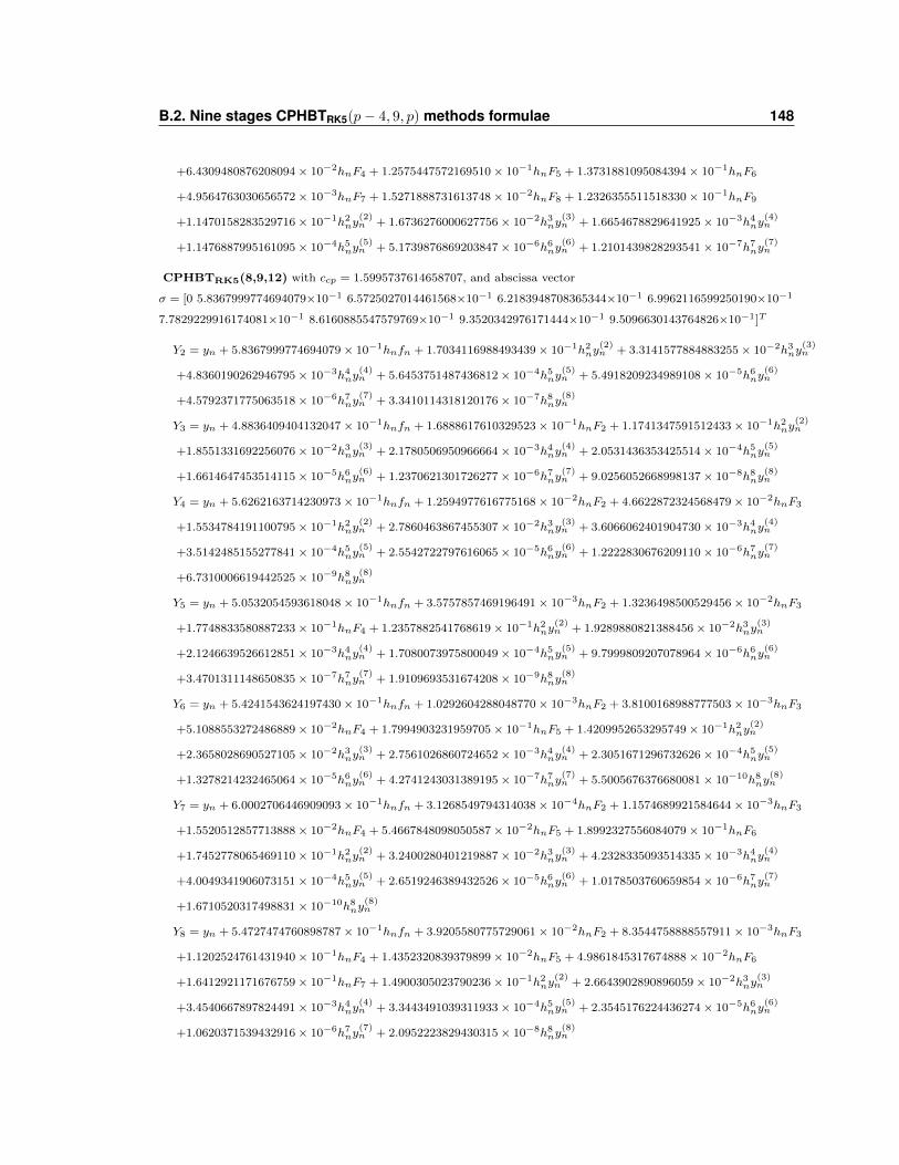
B.2. Nine stages CPHBTRK5(p− 4, 9, p) methods formulae 148
+6.4309480876208094× 10⁻²hnF4 + 1.2575447572169510× 10⁻¹hnF5 + 1.3731881095084394× 10⁻¹hnF6
+4.9564763030656572× 10⁻³hnF7 + 1.5271888731613748× 10⁻²hnF8 + 1.2326355511518330× 10⁻¹hnF9
+1.1470158283529716× 10⁻¹h2ny(2)n + 1.6736276000627756× 10⁻²h3ny
(3)n + 1.6654678829641925× 10⁻³h4ny
(4)n
+1.1476887995161095× 10⁻⁴h5ny(5)n + 5.1739876869203847× 10⁻⁶h6ny
(6)n + 1.2101439828293541× 10⁻⁷h7ny
(7)n
CPHBTRK5(8,9,12) with ccp = 1.5995737614658707, and abscissa vector
σ = [0 5.8367999774694079×10⁻¹ 6.5725027014461568×10⁻¹ 6.2183948708365344×10⁻¹ 6.9962116599250190×10⁻¹
7.7829229916174081×10⁻¹ 8.6160885547579769×10⁻¹ 9.3520342976171444×10⁻¹ 9.5096630143764826×10⁻¹]T
Y2 = yn + 5.8367999774694079× 10⁻¹hnfn + 1.7034116988493439× 10⁻¹h2ny(2)n + 3.3141577884883255× 10⁻²h3ny
(3)n
+4.8360190262946795× 10⁻³h4ny(4)n + 5.6453751487436812× 10⁻⁴h5ny
(5)n + 5.4918209234989108× 10⁻⁵h6ny
(6)n
+4.5792371775063518× 10⁻⁶h7ny(7)n + 3.3410114318120176× 10⁻⁷h8ny
(8)n
Y3 = yn + 4.8836409404132047× 10⁻¹hnfn + 1.6888617610329523× 10⁻¹hnF2 + 1.1741347591512433× 10⁻¹h2ny(2)n
+1.8551331692256076× 10⁻²h3ny(3)n + 2.1780506950966664× 10⁻³h4ny
(4)n + 2.0531436353425514× 10⁻⁴h5ny
(5)n
+1.6614647453514115× 10⁻⁵h6ny(6)n + 1.2370621301726277× 10⁻⁶h7ny
(7)n + 9.0256052668998137× 10⁻⁸h8ny
(8)n
Y4 = yn + 5.6262163714230973× 10⁻¹hnfn + 1.2594977616775168× 10⁻²hnF2 + 4.6622872324568479× 10⁻²hnF3
+1.5534784191100795× 10⁻¹h2ny(2)n + 2.7860463867455307× 10⁻²h3ny
(3)n + 3.6066062401904730× 10⁻³h4ny
(4)n
+3.5142485155277841× 10⁻⁴h5ny(5)n + 2.5542722797616065× 10⁻⁵h6ny
(6)n + 1.2222830676209110× 10⁻⁶h7ny
(7)n
+6.7310006619442525× 10⁻⁹h8ny(8)n
Y5 = yn + 5.0532054593618048× 10⁻¹hnfn + 3.5757857469196491× 10⁻³hnF2 + 1.3236498500529456× 10⁻²hnF3
+1.7748833580887233× 10⁻¹hnF4 + 1.2357882541768619× 10⁻¹h2ny(2)n + 1.9289880821388456× 10⁻²h3ny
(3)n
+2.1246639526612851× 10⁻³h4ny(4)n + 1.7080073975800049× 10⁻⁴h5ny
(5)n + 9.7999809207078964× 10⁻⁶h6ny
(6)n
+3.4701311148650835× 10⁻⁷h7ny(7)n + 1.9109693531674208× 10⁻⁹h8ny
(8)n
Y6 = yn + 5.4241543624197430× 10⁻¹hnfn + 1.0292604288048770× 10⁻³hnF2 + 3.8100168988777503× 10⁻³hnF3
+5.1088553272486889× 10⁻²hnF4 + 1.7994903231959705× 10⁻¹hnF5 + 1.4209952653295749× 10⁻¹h2ny(2)n
+2.3658028690527105× 10⁻²h3ny(3)n + 2.7561026860724652× 10⁻³h4ny
(4)n + 2.3051671296732626× 10⁻⁴h5ny
(5)n
+1.3278214232465064× 10⁻⁵h6ny(6)n + 4.2741243031389195× 10⁻⁷h7ny
(7)n + 5.5005676376680081× 10⁻¹⁰h8ny
(8)n
Y7 = yn + 6.0002706446909093× 10⁻¹hnfn + 3.1268549794314038× 10⁻⁴hnF2 + 1.1574689921584644× 10⁻³hnF3
+1.5520512857713888× 10⁻²hnF4 + 5.4667848098050587× 10⁻²hnF5 + 1.8992327556084079× 10⁻¹hnF6
+1.7452778065469110× 10⁻¹h2ny(2)n + 3.2400280401219887× 10⁻²h3ny
(3)n + 4.2328335093514335× 10⁻³h4ny
(4)n
+4.0049341906073151× 10⁻⁴h5ny(5)n + 2.6519246389432526× 10⁻⁵h6ny
(6)n + 1.0178503760659854× 10⁻⁶h7ny
(7)n
+1.6710520317498831× 10⁻¹⁰h8ny(8)n
Y8 = yn + 5.4727474760898787× 10⁻¹hnfn + 3.9205580775729061× 10⁻²hnF2 + 8.3544758888557911× 10⁻³hnF3
+1.1202524761431940× 10⁻¹hnF4 + 1.4352320839379899× 10⁻²hnF5 + 4.9861845317674888× 10⁻²hnF6
+1.6412921171676759× 10⁻¹hnF7 + 1.4900305023790236× 10⁻¹h2ny(2)n + 2.6643902890896059× 10⁻²h3ny
(3)n
+3.4540667897824491× 10⁻³h4ny(4)n + 3.3443491039311933× 10⁻⁴h5ny
(5)n + 2.3545176224436274× 10⁻⁵h6ny
(6)n
+1.0620371539432916× 10⁻⁶h7ny(7)n + 2.0952223829430315× 10⁻⁸h8ny
(8)n
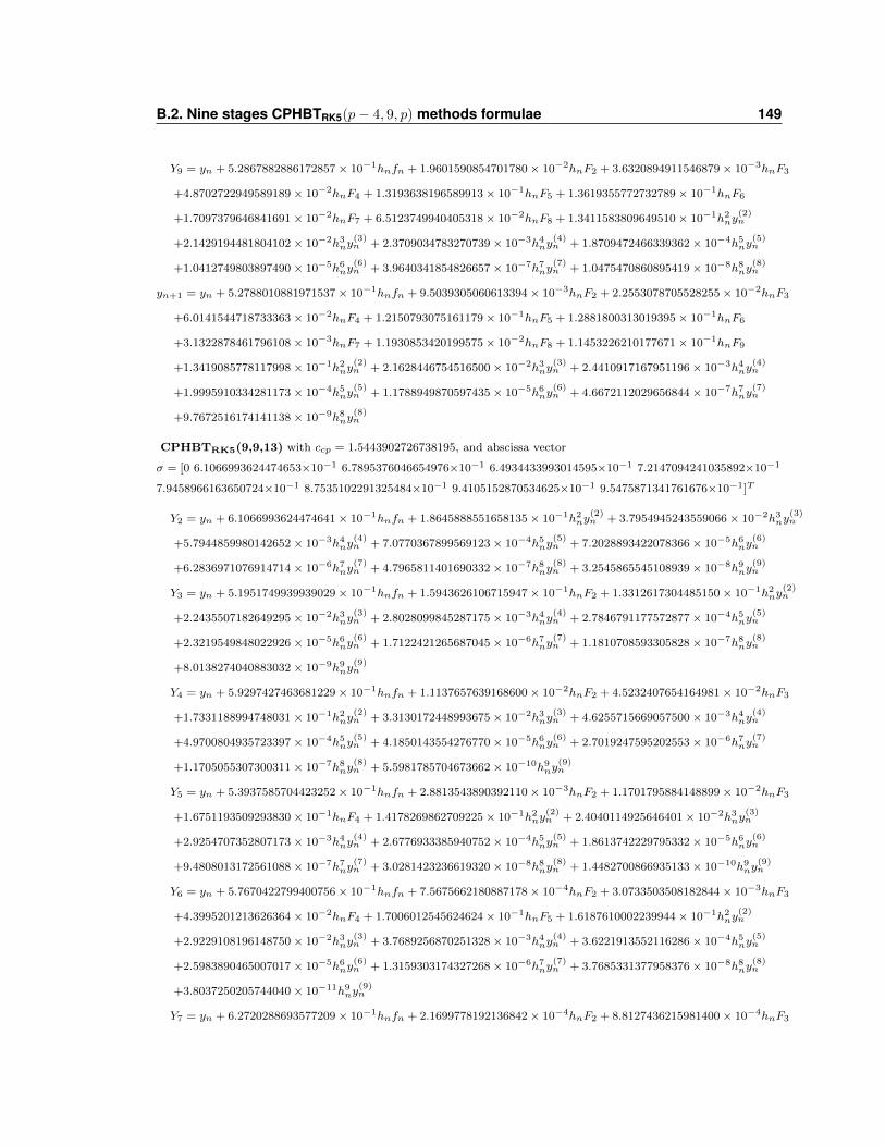
B.2. Nine stages CPHBTRK5(p− 4, 9, p) methods formulae 149
Y9 = yn + 5.2867882886172857× 10⁻¹hnfn + 1.9601590854701780× 10⁻²hnF2 + 3.6320894911546879× 10⁻³hnF3
+4.8702722949589189× 10⁻²hnF4 + 1.3193638196589913× 10⁻¹hnF5 + 1.3619355772732789× 10⁻¹hnF6
+1.7097379646841691× 10⁻²hnF7 + 6.5123749940405318× 10⁻²hnF8 + 1.3411583809649510× 10⁻¹h2ny(2)n
+2.1429194481804102× 10⁻²h3ny(3)n + 2.3709034783270739× 10⁻³h4ny
(4)n + 1.8709472466339362× 10⁻⁴h5ny
(5)n
+1.0412749803897490× 10⁻⁵h6ny(6)n + 3.9640341854826657× 10⁻⁷h7ny
(7)n + 1.0475470860895419× 10⁻⁸h8ny
(8)n
yn+1 = yn + 5.2788010881971537× 10⁻¹hnfn + 9.5039305060613394× 10⁻³hnF2 + 2.2553078705528255× 10⁻²hnF3
+6.0141544718733363× 10⁻²hnF4 + 1.2150793075161179× 10⁻¹hnF5 + 1.2881800313019395× 10⁻¹hnF6
+3.1322878461796108× 10⁻³hnF7 + 1.1930853420199575× 10⁻²hnF8 + 1.1453226210177671× 10⁻¹hnF9
+1.3419085778117998× 10⁻¹h2ny(2)n + 2.1628446754516500× 10⁻²h3ny
(3)n + 2.4410917167951196× 10⁻³h4ny
(4)n
+1.9995910334281173× 10⁻⁴h5ny(5)n + 1.1788949870597435× 10⁻⁵h6ny
(6)n + 4.6672112029656844× 10⁻⁷h7ny
(7)n
+9.7672516174141138× 10⁻⁹h8ny(8)n
CPHBTRK5(9,9,13) with ccp = 1.5443902726738195, and abscissa vector
σ = [0 6.1066993624474653×10⁻¹ 6.7895376046654976×10⁻¹ 6.4934433993014595×10⁻¹ 7.2147094241035892×10⁻¹
7.9458966163650724×10⁻¹ 8.7535102291325484×10⁻¹ 9.4105152870534625×10⁻¹ 9.5475871341761676×10⁻¹]T
Y2 = yn + 6.1066993624474641× 10⁻¹hnfn + 1.8645888551658135× 10⁻¹h2ny(2)n + 3.7954945243559066× 10⁻²h3ny
(3)n
+5.7944859980142652× 10⁻³h4ny(4)n + 7.0770367899569123× 10⁻⁴h5ny
(5)n + 7.2028893422078366× 10⁻⁵h6ny
(6)n
+6.2836971076914714× 10⁻⁶h7ny(7)n + 4.7965811401690332× 10⁻⁷h8ny
(8)n + 3.2545865545108939× 10⁻⁸h9ny
(9)n
Y3 = yn + 5.1951749939939029× 10⁻¹hnfn + 1.5943626106715947× 10⁻¹hnF2 + 1.3312617304485150× 10⁻¹h2ny(2)n
+2.2435507182649295× 10⁻²h3ny(3)n + 2.8028099845287175× 10⁻³h4ny
(4)n + 2.7846791177572877× 10⁻⁴h5ny
(5)n
+2.3219549848022926× 10⁻⁵h6ny(6)n + 1.7122421265687045× 10⁻⁶h7ny
(7)n + 1.1810708593305828× 10⁻⁷h8ny
(8)n
+8.0138274040883032× 10⁻⁹h9ny(9)n
Y4 = yn + 5.9297427463681229× 10⁻¹hnfn + 1.1137657639168600× 10⁻²hnF2 + 4.5232407654164981× 10⁻²hnF3
+1.7331188994748031× 10⁻¹h2ny(2)n + 3.3130172448993675× 10⁻²h3ny
(3)n + 4.6255715669057500× 10⁻³h4ny
(4)n
+4.9700804935723397× 10⁻⁴h5ny(5)n + 4.1850143554276770× 10⁻⁵h6ny
(6)n + 2.7019247595202553× 10⁻⁶h7ny
(7)n
+1.1705055307300311× 10⁻⁷h8ny(8)n + 5.5981785704673662× 10⁻¹⁰h9ny
(9)n
Y5 = yn + 5.3937585704423252× 10⁻¹hnfn + 2.8813543890392110× 10⁻³hnF2 + 1.1701795884148899× 10⁻²hnF3
+1.6751193509293830× 10⁻¹hnF4 + 1.4178269862709225× 10⁻¹h2ny(2)n + 2.4040114925646401× 10⁻²h3ny
(3)n
+2.9254707352807173× 10⁻³h4ny(4)n + 2.6776933385940752× 10⁻⁴h5ny
(5)n + 1.8613742229795332× 10⁻⁵h6ny
(6)n
+9.4808013172561088× 10⁻⁷h7ny(7)n + 3.0281423236619320× 10⁻⁸h8ny
(8)n + 1.4482700866935133× 10⁻¹⁰h9ny
(9)n
Y6 = yn + 5.7670422799400756× 10⁻¹hnfn + 7.5675662180887178× 10⁻⁴hnF2 + 3.0733503508182844× 10⁻³hnF3
+4.3995201213626364× 10⁻²hnF4 + 1.7006012545624624× 10⁻¹hnF5 + 1.6187610002239944× 10⁻¹h2ny(2)n
+2.9229108196148750× 10⁻²h3ny(3)n + 3.7689256870251328× 10⁻³h4ny
(4)n + 3.6221913552116286× 10⁻⁴h5ny
(5)n
+2.5983890465007017× 10⁻⁵h6ny(6)n + 1.3159303174327268× 10⁻⁶h7ny
(7)n + 3.7685331377958376× 10⁻⁸h8ny
(8)n
+3.8037250205744040× 10⁻¹¹h9ny(9)n
Y7 = yn + 6.2720288693577209× 10⁻¹hnfn + 2.1699778192136842× 10⁻⁴hnF2 + 8.8127436215981400× 10⁻⁴hnF3
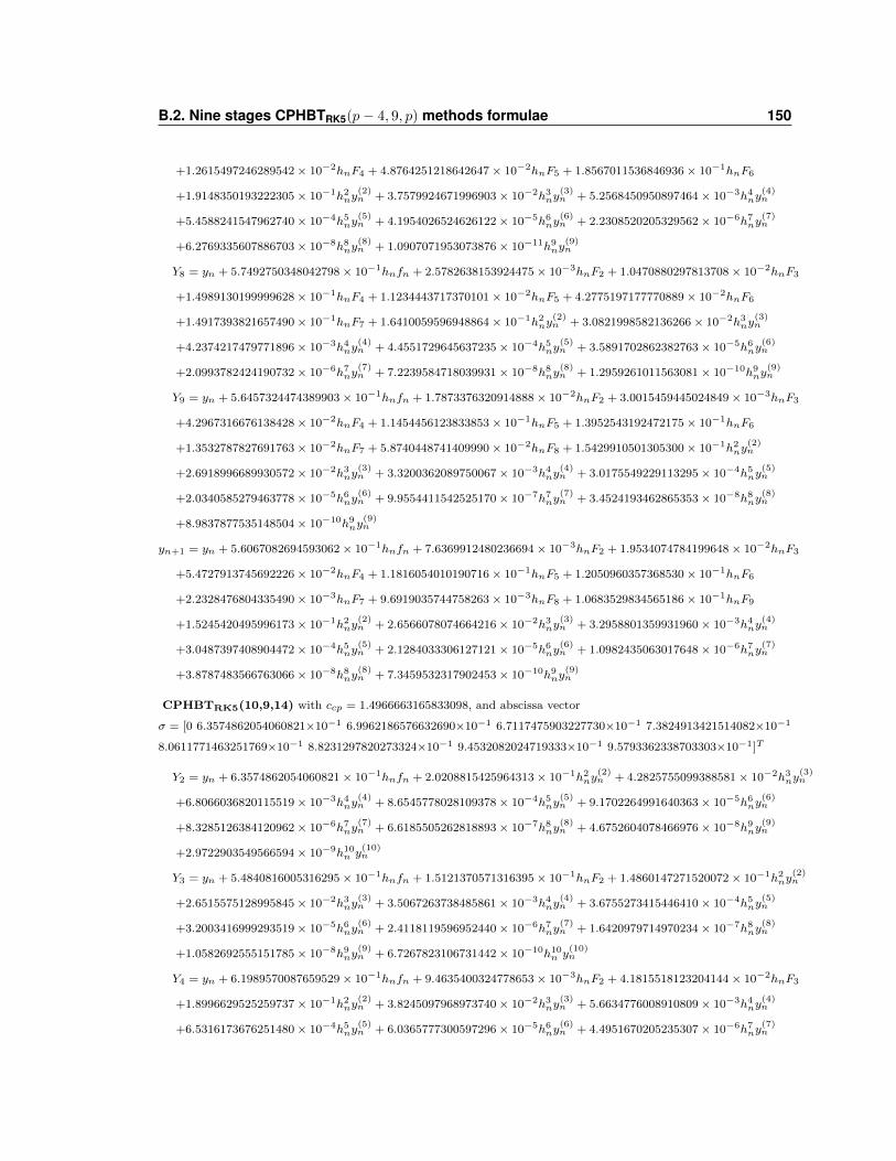
B.2. Nine stages CPHBTRK5(p− 4, 9, p) methods formulae 150
+1.2615497246289542× 10⁻²hnF4 + 4.8764251218642647× 10⁻²hnF5 + 1.8567011536846936× 10⁻¹hnF6
+1.9148350193222305× 10⁻¹h2ny(2)n + 3.7579924671996903× 10⁻²h3ny
(3)n + 5.2568450950897464× 10⁻³h4ny
(4)n
+5.4588241547962740× 10⁻⁴h5ny(5)n + 4.1954026524626122× 10⁻⁵h6ny
(6)n + 2.2308520205329562× 10⁻⁶h7ny
(7)n
+6.2769335607886703× 10⁻⁸h8ny(8)n + 1.0907071953073876× 10⁻¹¹h9ny
(9)n
Y8 = yn + 5.7492750348042798× 10⁻¹hnfn + 2.5782638153924475× 10⁻³hnF2 + 1.0470880297813708× 10⁻²hnF3
+1.4989130199999628× 10⁻¹hnF4 + 1.1234443717370101× 10⁻²hnF5 + 4.2775197177770889× 10⁻²hnF6
+1.4917393821657490× 10⁻¹hnF7 + 1.6410059596948864× 10⁻¹h2ny(2)n + 3.0821998582136266× 10⁻²h3ny
(3)n
+4.2374217479771896× 10⁻³h4ny(4)n + 4.4551729645637235× 10⁻⁴h5ny
(5)n + 3.5891702862382763× 10⁻⁵h6ny
(6)n
+2.0993782424190732× 10⁻⁶h7ny(7)n + 7.2239584718039931× 10⁻⁸h8ny
(8)n + 1.2959261011563081× 10⁻¹⁰h9ny
(9)n
Y9 = yn + 5.6457324474389903× 10⁻¹hnfn + 1.7873376320914888× 10⁻²hnF2 + 3.0015459445024849× 10⁻³hnF3
+4.2967316676138428× 10⁻²hnF4 + 1.1454456123833853× 10⁻¹hnF5 + 1.3952543192472175× 10⁻¹hnF6
+1.3532787827691763× 10⁻²hnF7 + 5.8740448741409990× 10⁻²hnF8 + 1.5429910501305300× 10⁻¹h2ny(2)n
+2.6918996689930572× 10⁻²h3ny(3)n + 3.3200362089750067× 10⁻³h4ny
(4)n + 3.0175549229113295× 10⁻⁴h5ny
(5)n
+2.0340585279463778× 10⁻⁵h6ny(6)n + 9.9554411542525170× 10⁻⁷h7ny
(7)n + 3.4524193462865353× 10⁻⁸h8ny
(8)n
+8.9837877535148504× 10⁻¹⁰h9ny(9)n
yn+1 = yn + 5.6067082694593062× 10⁻¹hnfn + 7.6369912480236694× 10⁻³hnF2 + 1.9534074784199648× 10⁻²hnF3
+5.4727913745692226× 10⁻²hnF4 + 1.1816054010190716× 10⁻¹hnF5 + 1.2050960357368530× 10⁻¹hnF6
+2.2328476804335490× 10⁻³hnF7 + 9.6919035744758263× 10⁻³hnF8 + 1.0683529834565186× 10⁻¹hnF9
+1.5245420495996173× 10⁻¹h2ny(2)n + 2.6566078074664216× 10⁻²h3ny
(3)n + 3.2958801359931960× 10⁻³h4ny
(4)n
+3.0487397408904472× 10⁻⁴h5ny(5)n + 2.1284033306127121× 10⁻⁵h6ny
(6)n + 1.0982435063017648× 10⁻⁶h7ny
(7)n
+3.8787483566763066× 10⁻⁸h8ny(8)n + 7.3459532317902453× 10⁻¹⁰h9ny
(9)n
CPHBTRK5(10,9,14) with ccp = 1.4966663165833098, and abscissa vector
σ = [0 6.3574862054060821×10⁻¹ 6.9962186576632690×10⁻¹ 6.7117475903227730×10⁻¹ 7.3824913421514082×10⁻¹
8.0611771463251769×10⁻¹ 8.8231297820273324×10⁻¹ 9.4532082024719333×10⁻¹ 9.5793362338703303×10⁻¹]T
Y2 = yn + 6.3574862054060821× 10⁻¹hnfn + 2.0208815425964313× 10⁻¹h2ny(2)n + 4.2825755099388581× 10⁻²h3ny
(3)n
+6.8066036820115519× 10⁻³h4ny(4)n + 8.6545778028109378× 10⁻⁴h5ny
(5)n + 9.1702264991640363× 10⁻⁵h6ny
(6)n
+8.3285126384120962× 10⁻⁶h7ny(7)n + 6.6185505262818893× 10⁻⁷h8ny
(8)n + 4.6752604078466976× 10⁻⁸h9ny
(9)n
+2.9722903549566594× 10⁻⁹h10n y(10)n
Y3 = yn + 5.4840816005316295× 10⁻¹hnfn + 1.5121370571316395× 10⁻¹hnF2 + 1.4860147271520072× 10⁻¹h2ny(2)n
+2.6515575128995845× 10⁻²h3ny(3)n + 3.5067263738485861× 10⁻³h4ny
(4)n + 3.6755273415446410× 10⁻⁴h5ny
(5)n
+3.2003416999293519× 10⁻⁵h6ny(6)n + 2.4118119596952440× 10⁻⁶h7ny
(7)n + 1.6420979714970234× 10⁻⁷h8ny
(8)n
+1.0582692555151785× 10⁻⁸h9ny(9)n + 6.7267823106731442× 10⁻¹⁰h10n y
(10)n
Y4 = yn + 6.1989570087659529× 10⁻¹hnfn + 9.4635400324778653× 10⁻³hnF2 + 4.1815518123204144× 10⁻²hnF3
+1.8996629525259737× 10⁻¹h2ny(2)n + 3.8245097968973740× 10⁻²h3ny
(3)n + 5.6634776008910809× 10⁻³h4ny
(4)n
+6.5316173676251480× 10⁻⁴h5ny(5)n + 6.0365777300597296× 10⁻⁵h6ny
(6)n + 4.4951670205235307× 10⁻⁶h7ny
(7)n
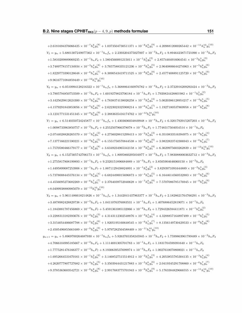
B.2. Nine stages CPHBTRK5(p− 4, 9, p) methods formulae 151
+2.6181694376066425× 10⁻⁷h8ny(8)n + 1.0373504730511371× 10⁻⁸h9ny
(9)n + 4.2098812000265442× 10⁻¹¹h10n y
(10)n
Y5 = yn + 5.6801307249977362× 10⁻¹hnfn + 2.2393204375027007× 10⁻³hnF2 + 9.8946423871721090× 10⁻³hnF3
+1.5810209889069235× 10⁻¹hnF4 + 1.5804560091215011× 10⁻¹h2ny(2)n + 2.8574404916064541× 10⁻²h3ny
(3)n
+3.7489778157134934× 10⁻³h4ny(4)n + 3.7657588335121236× 10⁻⁴h5ny
(5)n + 2.9640806644274963× 10⁻⁵h6ny
(6)n
+1.8229773390128648× 10⁻⁶h7ny(7)n + 8.3890543419711525× 10⁻⁸h8ny
(8)n + 2.4577408891125720× 10⁻⁹h9ny
(9)n
+9.9616771084859449× 10⁻¹²h10n y(10)n
Y6 = yn + 6.0510994128216322× 10⁻¹hnfn + 5.3688864160976782× 10⁻⁴hnF2 + 2.3722916209292424× 10⁻³hnF3
+3.7905794850753509× 10⁻²hnF4 + 1.6019279823706184× 10⁻¹hnF5 + 1.7920824428801982× 10⁻¹h2ny(2)n
+3.4425629812624300× 10⁻²h3ny(3)n + 4.7838374138026258× 10⁻³h4ny
(4)n + 5.0620386128954217× 10⁻⁴h5ny
(5)n
+4.1579291843853056× 10⁻⁵h6ny(6)n + 2.6223023325908214× 10⁻⁶h7ny
(7)n + 1.1927180537869958× 10⁻⁷h8ny
(8)n
+3.1231771531451345× 10⁻⁹h9ny(9)n + 2.3883635416174762× 10⁻¹²h10n y
(10)n
Y7 = yn + 6.5140350724245877× 10⁻¹hnfn + 1.4303606034849948× 10⁻⁴hnF2 + 6.3201792915207203× 10⁻⁴hnF3
+1.0098733963850757× 10⁻²hnF4 + 4.2552507966378078× 10⁻²hnF5 + 1.7748317504054514× 10⁻¹hnF6
+2.0744028826265570× 10⁻¹h2ny(2)n + 4.2756028815299413× 10⁻²h3ny
(3)n + 6.3510833516394975× 10⁻³h4ny
(4)n
+7.1377166221590221× 10⁻⁴h5ny(5)n + 6.1551750570844538× 10⁻⁵h6ny
(6)n + 3.9822823742306943× 10⁻⁶h7ny
(7)n
+1.7570580466179177× 10⁻⁷h8ny(8)n + 3.6349234965342158× 10⁻⁹h9ny
(9)n + 6.3629975603262839× 10⁻¹³h10n y
(10)n
Y8 = yn + 6.1527305742706173× 10⁻¹hnfn + 1.8095860295016977× 10⁻³hnF2 + 7.9830880003632712× 10⁻³hnF3
+1.2755817808199893× 10⁻¹hnF4 + 9.2320151896684889× 10⁻³hnF5 + 3.8505904646060150× 10⁻²hnF6
+1.4495899087253908× 10⁻¹hnF7 + 1.8871129438824891× 10⁻¹h2ny(2)n + 3.8293971091644889× 10⁻²h3ny
(3)n
+5.7378008445576134× 10⁻³h4ny(4)n + 6.6824490015696873× 10⁻⁴h5ny
(5)n + 6.1644614560532883× 10⁻⁵h6ny
(6)n
+4.4556095273682269× 10⁻⁶h7ny(7)n + 2.3764039752040628× 10⁻⁷h8ny
(8)n + 7.5707086785176945× 10⁻⁹h9ny
(9)n
+8.0499938880985079× 10⁻¹²h10n y(10)n
Y9 = yn + 5.9611486618214826× 10⁻¹hnfn + 1.3442041437963377× 10⁻²hnF2 + 2.1828621764766291× 10⁻³hnF3
+3.4878982428829738× 10⁻²hnF4 + 1.0411076376083531× 10⁻¹hnF5 + 1.4076886452819071× 10⁻¹hnF6
+1.1843881787456869× 10⁻²hnF7 + 5.4591361085132066× 10⁻²hnF8 + 1.7294326594411871× 10⁻¹h2ny(2)n
+3.2288313182393676× 10⁻²h3ny(3)n + 4.3143112302548876× 10⁻³h4ny
(4)n + 4.3288857164897499× 10⁻⁴h5ny
(5)n
+3.3154054406687788× 10⁻⁵h6ny(6)n + 1.9205195160648545× 10⁻⁶h7ny
(7)n + 8.1356149730429533× 10⁻⁸h8ny
(8)n
+2.4505496855661689× 10⁻⁹h9ny(9)n + 5.9797282504588469× 10⁻¹¹h10n y
(10)n
yn+1 = yn + 5.8969700264687930× 10⁻¹hnfn + 5.9263765358245945× 10⁻³hnF2 + 1.7599863961789489× 10⁻²hnF3
+4.7066104995185667× 10⁻²hnF4 + 1.1114691305701783× 10⁻¹hnF5 + 1.1831704599391640× 10⁻¹hnF6
+1.7775281476166377× 10⁻³hnF7 + 8.1930639537699974× 10⁻³hnF8 + 1.0027610070800021× 10⁻¹hnF9
+1.6952664531670161× 10⁻¹h2ny(2)n + 3.1468527515514912× 10⁻²h3ny
(3)n + 4.2053855785304135× 10⁻³h4ny
(4)n
+4.2620777807727682× 10⁻⁴h5ny(5)n + 3.3503944431217883× 10⁻⁵h6ny
(6)n + 2.0419345291708860× 10⁻⁶h7ny
(7)n
+9.3785363603542721× 10⁻⁸h8ny(8)n + 2.9917683775701943× 10⁻⁹h9ny
(9)n + 5.1763384829666555× 10⁻¹¹h10n y
(10)n
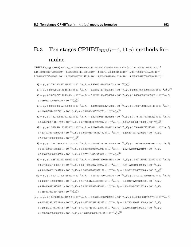
B.3. Ten stages CPHBTRK5(p− 4, 10, p) methods formulae 152
B.3 Ten stages CPHBTRK5(p−4, 10, p) methods for-
mulae
CPHBTRK5(2,10,6) with ccp = 3.5646029568785740, and abscissa vector σ = [0 2.7842964332218451×10⁻¹
4.1816904481179606×10⁻¹ 3.9067928644511601×10⁻¹ 3.8637915334868184×10⁻¹ 5.2647383807775272×10⁻¹
7.0948880078541965×10⁻¹ 8.6092081271814713×10⁻¹ 8.6331609198841319×10⁻¹ 9.2359094107564599×10⁻¹]T
Y2 = yn + 2.7842964332218451× 10⁻¹hnfn + 3.8761533140259471× 10⁻²h2ny(2)n
Y3 = yn + 2.0829660140341305× 10⁻¹hnfn + 2.0987244340838301× 10⁻¹hnF2 + 2.8997965458053533× 10⁻²h2ny(2)n
Y4 = yn + 2.0788727118384684× 10⁻¹hnfn + 7.8226619945594530× 10⁻²hnF2 + 1.0456539531567460× 10⁻¹hnF3
+1.0808531059356920× 10⁻²h2ny(2)n
Y5 = yn + 2.0035382524896286× 10⁻¹hnfn + 3.1407830653775524× 10⁻²hnF2 + 4.1982796017569143× 10⁻²hnF3
+1.1263470142837431× 10⁻¹hnF4 + 4.3396034925764770× 10⁻³h2ny(2)n
Y6 = yn + 1.7321599331601423× 10⁻¹hnfn + 2.3780494143120792× 10⁻²hnF2 + 3.1787347741816220× 10⁻²hnF3
+8.5281562014141582× 10⁻²hnF4 + 2.1240844086265992× 10⁻¹hnF5 + 3.2857384063319909× 10⁻³h2ny(2)n
Y7 = yn + 1.5228416193073463× 10⁻¹hnfn + 2.0906795741995821× 10⁻²hnF2 + 2.7946079775225816× 10⁻²hnF3
+7.4975910376689242× 10⁻²hnF4 + 1.8674043778337787× 10⁻¹hnF5 + 2.4663541517739626× 10⁻¹hnF6
+2.8886810050869206× 10⁻³h2ny(2)n
Y8 = yn + 1.7211789900772700× 10⁻¹hnfn + 1.7189877825122258× 10⁻²hnF2 + 2.2977681656987981× 10⁻²hnF3
+6.1646306545852791× 10⁻²hnF4 + 1.5354076014900933× 10⁻¹hnF5 + 2.0278729892720190× 10⁻¹hnF6
+2.3066098860624595× 10⁻¹hnF7 + 2.3751164054973081× 10⁻³h2ny(2)n
Y9 = yn + 1.8487661073348063× 10⁻¹hnfn + 1.1892874300183151× 10⁻¹hnF2 + 1.5897185683123877× 10⁻¹hnF3
+2.6573936974398974× 10⁻²hnF4 + 6.6186967022478962× 10⁻²hnF5 + 8.7415721100029306× 10⁻²hnF6
+9.9431260021363793× 10⁻²hnF7 + 1.2093099630359121× 10⁻¹hnF8 + 1.6432322059672003× 10⁻²h2ny(2)n
Y10 = yn + 1.8604197008738452× 10⁻¹hnfn + 9.5175947307226436× 10⁻²hnF2 + 1.2722153356038512× 10⁻¹hnF3
+4.4559371989602158× 10⁻²hnF4 + 8.1796442454806009× 10⁻²hnF5 + 1.0803176727439978× 10⁻¹hnF6
+9.4146663729170951× 10⁻²hnF7 + 5.6213339927445892× 10⁻²hnF8 + 1.3040390474522515× 10⁻¹hnF9
+1.3150410733447590× 10⁻²h2ny(2)n
yn+1 = yn + 1.8166312024945286× 10⁻¹hnfn + 6.3485441638502421× 10⁻²hnF2 + 8.4860886311297734× 10⁻²hnF3
+9.0655938213552140× 10⁻²hnF4 + 9.4477412549241357× 10⁻²hnF5 + 1.2474549960713693× 10⁻¹hnF6
+1.2862535040010073× 10⁻¹hnF7 + 4.1753746470125870× 10⁻²hnF8 + 6.0207984191906955× 10⁻²hnF9
+1.2952462036868309× 10⁻¹hnF10 + 1.0429630883138145× 10⁻²h2ny(2)n
B.3. Ten stages CPHBTRK5(p− 4, 10, p) methods formulae 153
CPHBTRK5(3,10,7) with ccp = 3.1200969859848842, and abscissa vector sigma = [0 3.2050285760086444×10⁻¹
4.4361640980594369×10⁻¹ 4.9699659275932151×10⁻¹ 4.3080263699822630×10⁻¹ 5.5962554634995565×10⁻¹
7.0303366569480485×10⁻¹ 8.3252919142375004×10⁻¹ 9.0103587809232788×10⁻¹ 9.2299674761687311×10⁻¹]T
Y2 = yn + 3.2050285760086444× 10⁻¹hnfn + 5.1361040865160010× 10⁻²h2ny(2)n + 5.4871201222128525× 10⁻³h3ny
(3)n
Y3 = yn + 2.3894270785911881× 10⁻¹hnfn + 2.0467370194682488× 10⁻¹hnF2 + 3.2799253174852494× 10⁻²h2ny(2)n
+4.0380325680298120× 10⁻³h3ny(3)n
Y4 = yn + 2.6384659966337665× 10⁻¹hnfn + 9.0864055769972821× 10⁻²hnF2 + 1.4228593732597206× 10⁻¹hnF3
+3.1260240397285581× 10⁻²h2ny(2)n + 1.7926681003588467× 10⁻³h3ny
(3)n
Y5 = yn + 3.0792904785269803× 10⁻¹hnfn + 2.0166165944127908× 10⁻²hnF2 + 3.1577735115338887× 10⁻²hnF3
+7.1129688086061446× 10⁻²hnF4 + 3.6972528105890981× 10⁻²h2ny(2)n + 3.9785928087344042× 10⁻⁴h3ny
(3)n
Y6 = yn + 2.5889870899479361× 10⁻¹hnfn + 1.3678009624687621× 10⁻²hnF2 + 2.1418080463590086× 10⁻²hnF3
+4.8244795809858680× 10⁻²hnF4 + 2.1738595145702558× 10⁻¹hnF5 + 2.5077182662621995× 10⁻²h2ny(2)n
+2.6985412537690751× 10⁻⁴h3ny(3)n
Y7 = yn + 2.4990868717298748× 10⁻¹hnfn + 9.9767410793949567× 10⁻³hnF2 + 1.5622349235462385× 10⁻²hnF3
+3.5189757094079489× 10⁻²hnF4 + 1.5856132664727501× 10⁻¹hnF5 + 2.3377480446560542× 10⁻¹hnF6
+2.0376083350789522× 10⁻²h2ny(2)n + 1.9683161600008567× 10⁻⁴h3ny
(3)n
Y8 = yn + 2.7201857717838834× 10⁻¹hnfn + 3.6032833524090833× 10⁻²hnF2 + 1.0729474639132179× 10⁻²hnF3
+2.4168426950863291× 10⁻²hnF4 + 1.0890037774518724× 10⁻¹hnF5 + 1.6055721182919455× 10⁻¹hnF6
+2.2012228955689364× 10⁻¹hnF7 + 2.6712536887582496× 10⁻²h2ny(2)n + 6.3476958226611768× 10⁻⁴h3ny
(3)n
Y9 = yn + 2.4715921561947546× 10⁻¹hnfn + 1.0217860189175355× 10⁻¹hnF2 + 1.3730578806730506× 10⁻¹hnF3
+1.2005028944805181× 10⁻²hnF4 + 5.4093391745733480× 10⁻²hnF5 + 7.9752562267518520× 10⁻²hnF6
+1.0933994433729180× 10⁻¹hnF7 + 1.5920134521844481× 10⁻¹hnF8 + 2.8962157560692869× 10⁻²h2ny(2)n
+1.9780802820534545× 10⁻³h3ny(3)n
Y10 = yn + 2.4695196732085400× 10⁻¹hnfn + 6.0181404002769251× 10⁻²hnF2 + 8.7664481989114793× 10⁻²hnF3
+7.7400070405320612× 10⁻²hnF4 + 7.6895109292245703× 10⁻²hnF5 + 1.1337026195981609× 10⁻¹hnF6
+1.2158190033865408× 10⁻¹hnF7 + 4.6114405330680071× 10⁻²hnF8 + 9.2837146977418517× 10⁻²hnF9
+2.5227343509045069× 10⁻²h2ny(2)n + 1.1763728132955210× 10⁻³h3ny
(3)n
yn+1 = yn + 2.5830759520583763× 10⁻¹hnfn + 4.3428428180664114× 10⁻²hnF2 + 6.4984111796381180× 10⁻²hnF3
+9.1206283256506898× 10⁻²hnF4 + 8.9121350143994416× 10⁻²hnF5 + 1.0855393058951872× 10⁻¹hnF6
+1.3327288860399417× 10⁻¹hnF7 + 2.1190182583713087× 10⁻²hnF8 + 4.2659903795695203× 10⁻²hnF9
+1.4727532584369460× 10⁻¹hnF10 + 2.7071045291873909× 10⁻²h2ny(2)n + 1.1793895663086526× 10⁻³h3ny
(3)n
CPHBTRK5(4,10,8) with ccp = 2.6736188344238125, and abscissa vector σ = [0 3.7402489357294960×10⁻¹
4.9449816435270666×10⁻¹ 4.9878873711571220×10⁻¹ 5.0283264680252127×10⁻¹ 6.2541121459979643×10⁻¹
7.3668628792253987×10⁻¹ 8.4269412254028120×10⁻¹ 9.1992200220240106×10⁻¹ 9.3148685278833943×10⁻¹]T
Y2 = yn + 3.7402489357294960× 10⁻¹hnfn + 6.9947310506128138× 10⁻²h2ny(2)n + 8.7206784559228766× 10⁻³h3ny
(3)n
B.3. Ten stages CPHBTRK5(p− 4, 10, p) methods formulae 154
+8.1543770784011716× 10⁻⁴h4ny(4)n
Y3 = yn + 2.7840897317942642× 10⁻¹hnfn + 2.1608919117328024× 10⁻¹hnF2 + 4.1441480543247346× 10⁻²h2ny(2)n
+5.0382859173385046× 10⁻³h3ny(3)n + 6.0697878358535848× 10⁻⁴h4ny
(4)n
Y4 = yn + 3.4704003821033153× 10⁻¹hnfn + 5.5567651163863953× 10⁻²hnF2 + 9.6181047741516729× 10⁻²hnF3
+5.6050065770380464× 10⁻²h2ny(2)n + 5.0359836972812223× 10⁻³h3ny
(3)n + 1.5608548084707833× 10⁻⁴h4ny
(4)n
Y5 = yn + 3.6705629478183960× 10⁻¹hnfn + 1.4349851482314973× 10⁻²hnF2 + 2.4837899777951287× 10⁻²hnF3
+9.6588600760415450× 10⁻²hnF4 + 6.0593531632119314× 10⁻²h2ny(2)n + 5.1337551944944755× 10⁻³h3ny
(3)n
+4.0307686608820573× 10⁻⁵h4ny(4)n
Y6 = yn + 3.2186672374877234× 10⁻¹hnfn + 8.5441500969952264× 10⁻³hnF2 + 1.4788915694248303× 10⁻²hnF3
+5.7510525706333054× 10⁻²hnF4 + 2.2270089935344747× 10⁻¹hnF5 + 4.4393892024205163× 10⁻²h2ny(2)n
+3.0567267540746335× 10⁻³h3ny(3)n + 9.3670480396297045× 10⁻⁵h4ny
(4)n
Y7 = yn + 3.4472015925654997× 10⁻¹hnfn + 1.6078577223738736× 10⁻²hnF2 + 8.3090577508470979× 10⁻³hnF3
+3.2311921256089532× 10⁻²hnF4 + 1.2512307677925649× 10⁻¹hnF5 + 2.1014349565605805× 10⁻¹hnF6
+5.0771852337739710× 10⁻²h2ny(2)n + 3.5583179514058717× 10⁻³h3ny
(3)n + 7.7216333997365640× 10⁻⁵h4ny
(4)n
Y8 = yn + 3.5804520915881827× 10⁻¹hnfn + 7.5726447810212802× 10⁻²hnF2 + 4.5308761104523735× 10⁻³hnF3
+1.7619484241412197× 10⁻²hnF4 + 6.8228814438993993× 10⁻²hnF5 + 1.1458990571318592× 10⁻¹hnF6
+2.0395338506720576× 10⁻¹hnF7 + 5.9491055666249036× 10⁻²h2ny(2)n + 5.3156914161634631× 10⁻³h3ny
(3)n
+1.8808733796739743× 10⁻⁴h4ny(4)n
Y9 = yn + 3.0622827155293281× 10⁻¹hnfn + 1.1786919340158487× 10⁻¹hnF2 + 1.0726270981899948× 10⁻¹hnF3
+1.4380399058469868× 10⁻²hnF4 + 5.5685942078426302× 10⁻²hnF5 + 6.7279099082940677× 10⁻²hnF6
+8.8647678380208539× 10⁻²hnF7 + 1.6256870882883856× 10⁻¹hnF8 + 4.6449201078373012× 10⁻²h2ny(2)n
+4.6252927899254970× 10⁻³h3ny(3)n + 3.0847116933835497× 10⁻⁴h4ny
(4)n
Y10 = yn + 3.2864696617127187× 10⁻¹hnfn + 3.1151576604196412× 10⁻²hnF2 + 3.0012731014500662× 10⁻²hnF3
+3.0863431686783370× 10⁻²hnF4 + 1.1951401781436777× 10⁻¹hnF5 + 1.9512862937953399× 10⁻¹hnF6
+8.1787714230854527× 10⁻²hnF7 + 3.4653598481100327× 10⁻²hnF8 + 7.9728187405730497× 10⁻²hnF9
+4.7017672666169102× 10⁻²h2ny(2)n + 3.5126209425953032× 10⁻³h3ny
(3)n + 1.1516521344988865× 10⁻⁴h4ny
(4)n
yn+1 = yn + 3.2427827894719286× 10⁻¹hnfn + 3.3842469714701388× 10⁻²hnF2 + 4.5121298517174925× 10⁻²hnF3
+6.1887573202160040× 10⁻²hnF4 + 1.1369218819461296× 10⁻¹hnF5 + 1.2177771423612925× 10⁻¹hnF6
+1.1828871171632893× 10⁻¹hnF7 + 1.2850304192812181× 10⁻²hnF8 + 2.9564937143943128× 10⁻²hnF9
+1.3869652413494440× 10⁻¹hnF10 + 4.6469585328660794× 10⁻²h2ny(2)n + 3.5534596678701018× 10⁻³h3ny
(3)n
+1.2558765850119953× 10⁻⁴h4ny(4)n
CPHBTRK5(5,10,9) with ccp = 2.3856368028474391, and abscissa vector σ = [0 4.1917529055823749×10⁻¹
5.2405698244208032×10⁻¹ 5.2786402398851617×10⁻¹ 5.5210608401389483×10⁻¹ 6.6238678709395604×10⁻¹
7.5564179985879198×10⁻¹ 8.7471065097018452×10⁻¹ 9.1293992993193451×10⁻¹ 9.4085301374204600×10⁻¹]T
Y2 = yn + 4.1917529055823749× 10⁻¹hnfn + 8.7853962107291420× 10⁻²h2ny(2)n + 1.2275403364338754× 10⁻²h3ny
(3)n
B.3. Ten stages CPHBTRK5(p− 4, 10, p) methods formulae 155
+1.2863864429915658× 10⁻³h4ny(4)n + 1.0784428220223343× 10⁻⁴h5ny
(5)n
Y3 = yn + 3.1927855855928888× 10⁻¹hnfn + 2.0477842388279147× 10⁻¹hnF2 + 5.1479805092022442× 10⁻²h2ny(2)n
+5.9968652973965393× 10⁻³h3ny(3)n + 6.2896137839045377× 10⁻⁴h4ny
(4)n + 6.5966496453727342× 10⁻⁵h5ny
(5)n
Y4 = yn + 3.9845683886584027× 10⁻¹hnfn + 4.2470777551617149× 10⁻²hnF2 + 8.6936407571058749× 10⁻²hnF3
+7.5957881974197103× 10⁻²h2ny(2)n + 8.8448953503901511× 10⁻³h3ny
(3)n + 6.2829070580332420× 10⁻⁴h4ny
(4)n
+1.3681365173263413× 10⁻⁵h5ny(5)n
Y5 = yn + 4.1395781011349519× 10⁻¹hnfn + 1.0695319063338957× 10⁻²hnF2 + 2.1892997274723675× 10⁻²hnF3
+1.0555995756233706× 10⁻¹hnF4 + 8.0732868467274163× 10⁻²h2ny(2)n + 9.3963716502202723× 10⁻³h3ny
(3)n
+6.2734856233036425× 10⁻⁴h4ny(4)n + 3.4453469935243566× 10⁻⁶h5ny
(5)n
Y6 = yn + 3.7635523717243458× 10⁻¹hnfn + 5.4890890744295475× 10⁻³hnF2 + 1.1236000668659346× 10⁻²hnF3
+5.4175850792410128× 10⁻²hnF4 + 2.1513060938602241× 10⁻¹hnF5 + 6.3816531843595342× 10⁻²h2ny(2)n
+6.0766139965727026× 10⁻³h3ny(3)n + 3.2197002435864144× 10⁻⁴h4ny
(4)n + 1.2107854095285966× 10⁻⁵h5ny
(5)n
Y7 = yn + 3.9987371489811863× 10⁻¹hnfn + 4.0363174140173659× 10⁻²hnF2 + 5.0647418645017161× 10⁻³hnF3
+2.4420317125707088× 10⁻²hnF4 + 9.6972315668539366× 10⁻²hnF5 + 1.8894753616175156× 10⁻¹hnF6
+7.4337842526428721× 10⁻²h2ny(2)n + 8.0368721906856969× 10⁻³h3ny
(3)n + 4.9701743471249754× 10⁻⁴h4ny
(4)n
+1.5205695046221745× 10⁻⁵h5ny(5)n
Y8 = yn + 4.0872238091506313× 10⁻¹hnfn + 6.8170982705768782× 10⁻²hnF2 + 2.7428480455627701× 10⁻³hnF3
+1.3225001568141824× 10⁻²hnF4 + 5.2516067673533284× 10⁻²hnF5 + 1.0232592186139944× 10⁻¹hnF6
+2.2700744820071542× 10⁻¹hnF7 + 7.7255262932959409× 10⁻²h2ny(2)n + 8.0725948047622696× 10⁻³h3ny
(3)n
+4.1128808277233618× 10⁻⁴h4ny(4)n + 2.0149783909574135× 10⁻⁵h5ny
(5)n
Y9 = yn + 3.6632244181168760× 10⁻¹hnfn + 6.3506989130738406× 10⁻²hnF2 + 1.5193797672158917× 10⁻²hnF3
+3.9514679317807250× 10⁻²hnF4 + 1.5691155592380779× 10⁻¹hnF5 + 9.4680692606829001× 10⁻²hnF6
+6.2114217982995774× 10⁻²hnF7 + 1.1469555548590983× 10⁻¹hnF8 + 6.4679715890237882× 10⁻²h2ny(2)n
+7.3483179241706914× 10⁻³h3ny(3)n + 5.8373042939625420× 10⁻⁴h4ny
(4)n + 1.9155773629254956× 10⁻⁵h5ny
(5)n
Y10 = yn + 3.9009898424943285× 10⁻¹hnfn + 1.9829294933082171× 10⁻²hnF2 + 7.9048999082521332× 10⁻³hnF3
+3.1105251357254757× 10⁻²hnF4 + 1.2351798046019984× 10⁻¹hnF5 + 1.9683080587195864× 10⁻¹hnF6
+6.0671517984667363× 10⁻²hnF7 + 2.3824265778407835× 10⁻²hnF8 + 8.7070013198790513× 10⁻²hnF9
+6.8980165700845669× 10⁻²h2ny(2)n + 6.9204899744523193× 10⁻³h3ny
(3)n + 3.9302518860676939× 10⁻⁴h4ny
(4)n
+1.0207238601932514× 10⁻⁵h5ny(5)n
yn+1 = yn + 3.7969414299658161× 10⁻¹hnfn + 3.0786519618046827× 10⁻²hnF2 + 2.9936545631869378× 10⁻²hnF3
+3.5350898317343823× 10⁻²hnF4 + 1.4037731177484225× 10⁻¹hnF5 + 1.0479447431208680× 10⁻¹hnF6
+1.1882430037345164× 10⁻¹hnF7 + 7.2018856995588751× 10⁻³hnF8 + 2.6320571166776104× 10⁻²hnF9
+1.2671335010944271× 10⁻¹hnF10 + 6.6492573396444224× 10⁻²h2ny(2)n + 6.8100997046303853× 10⁻³h3ny
(3)n
+4.1580497337864356× 10⁻⁴h4ny(4)n + 1.2435129293901815× 10⁻⁵h5ny
(5)n
B.3. Ten stages CPHBTRK5(p− 4, 10, p) methods formulae 156
CPHBTRK5(6,10,10) with ccp = 2.1720633064988792, and abscissa vector σ = [0 4.6039173766619429×10⁻¹
5.5302830860306673×10⁻¹ 5.6209265279347487×10⁻¹ 5.9225669436654071×10⁻¹ 6.8850812576069620×10⁻¹
7.7342683799476519×10⁻¹ 8.7769081324673848×10⁻¹ 9.0825588600218488×10⁻¹ 9.4767740940606027×10⁻¹]T
Y2 = yn + 4.6039173766619429× 10⁻¹hnfn + 1.0598027605564893× 10⁻¹h2ny(2)n + 1.6264147817201060× 10⁻²h3ny
(3)n
+1.8719698188052591× 10⁻³h4ny(4)n + 1.7236788754768480× 10⁻⁴h5ny
(5)n + 1.3226125210988296× 10⁻⁵h6ny
(6)n
Y3 = yn + 3.6132178875054827× 10⁻¹hnfn + 1.9170651985251846× 10⁻¹hnF2 + 6.4660057261344620× 10⁻²h2ny(2)n
+7.8726150054111484× 10⁻³h3ny(3)n + 7.7948579410064224× 10⁻⁴h4ny
(4)n + 7.2208891059488535× 10⁻⁵h5ny
(5)n
+6.6889816437436232× 10⁻⁶h6ny(6)n
Y4 = yn + 4.4217295214897484× 10⁻¹hnfn + 3.5254487688933786× 10⁻²hnF2 + 8.4665212955566269× 10⁻²hnF3
+9.4920940796228037× 10⁻²h2ny(2)n + 1.2915391162833080× 10⁻²h3ny
(3)n + 1.1992281429935860× 10⁻³h4ny
(4)n
+7.1610561278309339× 10⁻⁵h5ny(5)n + 1.2300917949620015× 10⁻⁶h6ny
(6)n
Y5 = yn + 4.5622205129411858× 10⁻¹hnfn + 1.1288866968807590× 10⁻²hnF2 + 1.9377108551817013× 10⁻²hnF3
+1.0536866755179752× 10⁻¹hnF4 + 1.0024365149740622× 10⁻¹h2ny(2)n + 1.3819049751153016× 10⁻²h3ny
(3)n
+1.2779774284152013× 10⁻³h4ny(4)n + 7.2338199563864983× 10⁻⁵h5ny
(5)n + 3.7403959923412801× 10⁻⁷h6ny
(6)n
Y6 = yn + 4.2936992760642373× 10⁻¹hnfn + 4.9048411337496416× 10⁻³hnF2 + 8.4190591793399383× 10⁻³hnF3
+4.5781084695607766× 10⁻²hnF4 + 2.0003321314557515× 10⁻¹hnF5 + 8.5903372303297323× 10⁻²h2ny(2)n
+1.0275017622930144× 10⁻²h3ny(3)n + 7.6507879351271992× 10⁻⁴h4ny
(4)n + 3.1429848340212647× 10⁻⁵h5ny
(5)n
+6.0074457683547491× 10⁻⁷h6ny(6)n
Y7 = yn + 4.3300381569011170× 10⁻¹hnfn + 6.6435740383584810× 10⁻²hnF2 + 3.2278675322640863× 10⁻³hnF3
+1.7552469193160541× 10⁻²hnF4 + 7.6692739691321274× 10⁻²hnF5 + 1.7651420550432273× 10⁻¹hnF6
+8.9903601519914320× 10⁻²h2ny(2)n + 1.1513548428163798× 10⁻²h3ny
(3)n + 9.6126300509783737× 10⁻⁴h4ny
(4)n
+5.0430435551193395× 10⁻⁵h5ny(5)n + 2.0848667576175740× 10⁻⁶h6ny
(6)n
Y8 = yn + 4.4785330301293264× 10⁻¹hnfn + 9.3632253191585371× 10⁻²hnF2 + 1.4777465102325000× 10⁻³hnF3
+8.0356767546666610× 10⁻³hnF4 + 3.5110619412418026× 10⁻²hnF5 + 8.0809775674879417× 10⁻²hnF6
+2.1077143869002393× 10⁻¹hnF7 + 9.7280061614219523× 10⁻²h2ny(2)n + 1.2916217297737793× 10⁻²h3ny
(3)n
+1.0597905552383016× 10⁻³h4ny(4)n + 4.6755707895646095× 10⁻⁵h5ny
(5)n + 2.7705782652093099× 10⁻⁶h6ny
(6)n
Y9 = yn + 4.1549387261441162× 10⁻¹hnfn + 2.3647591471200748× 10⁻²hnF2 + 7.6569321725213878× 10⁻³hnF3
+4.1636797275277970× 10⁻²hnF4 + 1.8192540433328505× 10⁻¹hnF5 + 9.9086850141829316× 10⁻²hnF6
+4.3591268426073013× 10⁻²hnF7 + 9.5217169567585858× 10⁻²hnF8 + 8.0684451450822189× 10⁻²h2ny(2)n
+9.5144845480209968× 10⁻³h3ny(3)n + 7.4156466535279196× 10⁻⁴h4ny
(4)n + 3.8631835160384212× 10⁻⁵h5ny
(5)n
+7.9331697678630540× 10⁻⁷h6ny(6)n
Y10 = yn + 4.3763390277249853× 10⁻¹hnfn + 9.2120730972329069× 10⁻³hnF2 + 5.2018171784455136× 10⁻³hnF3
+2.8101541238680864× 10⁻²hnF4 + 1.2278524254092209× 10⁻¹hnF5 + 2.1155264271500743× 10⁻¹hnF6
+9.6894653137520586× 10⁻³hnF7 + 2.1164868449822866× 10⁻²hnF8 + 1.0233585609969797× 10⁻¹hnF9
+8.8739109617458012× 10⁻²h2ny(2)n + 1.0702065220994247× 10⁻²h3ny
(3)n + 8.0838842151547666× 10⁻⁴h4ny
(4)n
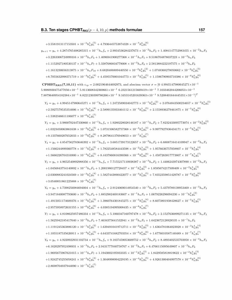
B.3. Ten stages CPHBTRK5(p− 4, 10, p) methods formulae 157
+3.5581913117153501× 10⁻⁵h5ny(5)n + 4.7936445753874328× 10⁻⁷h6ny
(6)n
yn+1 = yn + 4.2874765408285315× 10⁻¹hnfn + 2.9934536284237673× 10⁻²hnF2 + 1.4084147752983455× 10⁻²hnF3
+3.2263306724999316× 10⁻²hnF4 + 1.4096941900277368× 10⁻¹hnF5 + 9.5186704878037223× 10⁻²hnF6
+1.1152927180530137× 10⁻¹hnF7 + 5.3387686834779008× 10⁻³hnF8 + 2.5813884222197575× 10⁻²hnF9
+1.1613230656313875× 10⁻¹hnF10 + 8.6820488889440550× 10⁻²h2ny(2)n + 1.0748368278050662× 10⁻²h3ny
(3)n
+8.7055632998371719× 10⁻⁴h4ny(4)n + 4.4595570001044773× 10⁻⁵h5ny
(5)n + 1.1596790903710386× 10⁻⁶h6ny
(6)n
CPHBTRK5(7,10,11) with ccp = 2.0021964644692973, and abscissa vector σ = [0 4.9945147980645271×10⁻¹
5.9080930475477056×10⁻¹ 5.9113608342369661×10⁻¹ 6.2321561215669419×10⁻¹ 7.1033462044206053×10⁻¹
7.8879640954182384×10⁻¹ 8.8221230399786266×10⁻¹ 9.1653145201639363×10⁻¹ 9.5208401644445351×10⁻¹]T
Y2 = yn + 4.9945147980645271× 10⁻¹hnfn + 1.2472589034042773× 10⁻¹h2ny(2)n + 2.0764843500234657× 10⁻²h3ny
(3)n
+2.5927579535354006× 10⁻³h4ny(4)n + 2.5899135933464112× 10⁻⁴h5ny
(5)n + 2.1558936279461875× 10⁻⁵h6ny
(6)n
+1.5382346611186077× 10⁻⁶h7ny(7)n
Y3 = yn + 3.9800702447330860× 10⁻¹hnfn + 1.9280228028146187× 10⁻¹hnF2 + 7.8232433095773074× 10⁻²h2ny(2)n
+1.0323450063861638× 10⁻²h3ny(3)n + 1.0731506582757368× 10⁻³h4ny
(4)n + 9.9977927836434171× 10⁻⁵h5ny
(5)n
+9.1337660207652033× 10⁻⁶h6ny(6)n + 8.2879641376949653× 10⁻⁷h7ny
(7)n
Y4 = yn + 4.8547562783646392× 10⁻¹hnfn + 3.6851739173122657× 10⁻²hnF2 + 6.8808716414109947× 10⁻²hnF3
+1.1566244899360778× 10⁻¹h2ny(2)n + 1.7822548584443598× 10⁻²h3ny
(3)n + 1.9576636757058807× 10⁻³h4ny
(4)n
+1.5666226704316900× 10⁻⁴h5ny(5)n + 8.4437860816390366× 10⁻⁶h6ny
(6)n + 1.4587263817773807× 10⁻⁷h7ny
(7)n
Y5 = yn + 4.9652540892988356× 10⁻¹hnfn + 7.7155217110938387× 10⁻³hnF2 + 1.4406243974307890× 10⁻²hnF3
+1.0456843754140892× 10⁻¹hnF4 + 1.2001980127728457× 10⁻¹h2ny(2)n + 1.8595674217509409× 10⁻²h3ny
(3)n
+2.0300883241024569× 10⁻³h4ny(4)n + 1.5827443890422077× 10⁻⁴h5ny
(5)n + 7.8352359851429787× 10⁻⁶h6ny
(6)n
+3.0540851861225888× 10⁻⁸h7ny(7)n
Y6 = yn + 4.7398256984694004× 10⁻¹hnfn + 2.9124069014954540× 10⁻³hnF2 + 5.4379789139953469× 10⁻³hnF3
+3.9471840087793600× 10⁻²hnF4 + 1.8852982469183607× 10⁻¹hnF5 + 1.0679226296094230× 10⁻¹h2ny(2)n
+1.4915051174609376× 10⁻²h3ny(3)n + 1.3960764301845275× 10⁻³h4ny
(4)n + 8.6073801938428627× 10⁻⁵h5ny
(5)n
+2.9575958972631555× 10⁻⁶h6ny(6)n + 4.0385194995008435× 10⁻⁸h7ny
(7)n
Y7 = yn + 4.8108625957486334× 10⁻¹hnfn + 5.1060347160797478× 10⁻²hnF2 + 2.1527636899271135× 10⁻³hnF3
+1.5625942185417640× 10⁻²hnF4 + 7.4634375641532941× 10⁻²hnF5 + 1.6423672128928535× 10⁻¹hnF6
+1.1191245363886120× 10⁻¹h2ny(2)n + 1.6394910419712711× 10⁻²h3ny
(3)n + 1.6364781064023928× 10⁻³h4ny
(4)n
+1.1055187535626911× 10⁻⁴h5ny(5)n + 4.6433741682703354× 10⁻⁶h6ny
(6)n + 1.6776010587140489× 10⁻⁷h7ny
(7)n
Y8 = yn + 4.9220922931102734× 10⁻¹hnfn + 9.1837459053609752× 10⁻²hnF2 + 8.4893402535703958× 10⁻⁴hnF3
+6.1620297952498931× 10⁻³hnF4 + 2.9431777040758767× 10⁻²hnF5 + 6.4766115095649807× 10⁻²hnF6
+1.9695675967621015× 10⁻¹hnF7 + 1.1943002195933335× 10⁻¹h2ny(2)n + 1.8429585818819622× 10⁻²h3ny
(3)n
+1.9242745255058241× 10⁻³h4ny(4)n + 1.3048998994229195× 10⁻⁴h5ny
(5)n + 4.9261300404997578× 10⁻⁶h6ny
(6)n
+2.8698704937944090× 10⁻⁷h7ny(7)n
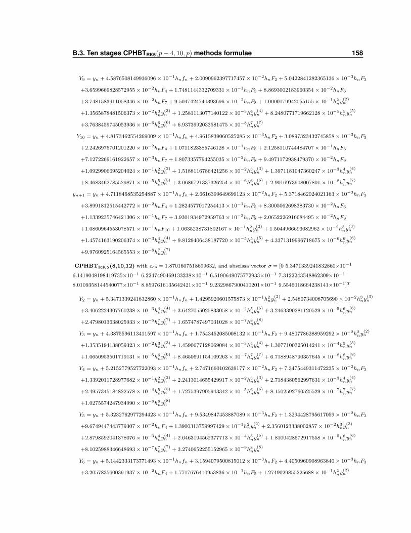
B.3. Ten stages CPHBTRK5(p− 4, 10, p) methods formulae 158
Y9 = yn + 4.5876508149936096× 10⁻¹hnfn + 2.0090962397717457× 10⁻²hnF2 + 5.0422841282365136× 10⁻³hnF3
+3.6599669828572955× 10⁻²hnF4 + 1.7481144332709331× 10⁻¹hnF5 + 8.8693002183960354× 10⁻²hnF6
+3.7481583911058346× 10⁻²hnF7 + 9.5047424740393696× 10⁻²hnF8 + 1.0000179942055155× 10⁻¹h2ny(2)n
+1.3565878481506373× 10⁻²h3ny(3)n + 1.2581113077140122× 10⁻³h4ny
(4)n + 8.2480771719662128× 10⁻⁵h5ny
(5)n
+3.7638459745053936× 10⁻⁶h6ny(6)n + 6.9373992033581475× 10⁻⁸h7ny
(7)n
Y10 = yn + 4.8173462554269009× 10⁻¹hnfn + 4.9615839060525285× 10⁻³hnF2 + 3.0897323432745858× 10⁻³hnF3
+2.2426975701201220× 10⁻²hnF4 + 1.0711823385746128× 10⁻¹hnF5 + 2.1258110744484707× 10⁻¹hnF6
+7.1272269161922657× 10⁻³hnF7 + 1.8073357794255035× 10⁻²hnF8 + 9.4971172938479370× 10⁻²hnF9
+1.0929906695204024× 10⁻¹h2ny(2)n + 1.5188116786421256× 10⁻²h3ny
(3)n + 1.3971181047360247× 10⁻³h4ny
(4)n
+8.4683462785529871× 10⁻⁵h5ny(5)n + 3.0686721337326254× 10⁻⁶h6ny
(6)n + 2.9016973908007801× 10⁻⁸h7ny
(7)n
yn+1 = yn + 4.7118468535254887× 10⁻¹hnfn + 2.6616399649699123× 10⁻²hnF2 + 5.3718462024021163× 10⁻³hnF3
+3.8991812515442772× 10⁻²hnF4 + 1.2824577017254413× 10⁻¹hnF5 + 8.3005062698383730× 10⁻²hnF6
+1.1339235746421306× 10⁻¹hnF7 + 3.9301934972959763× 10⁻³hnF8 + 2.0652226916684495× 10⁻²hnF9
+1.0860964553078571× 10⁻¹hnF10 + 1.0635238731802167× 10⁻¹h2ny(2)n + 1.5044966693082962× 10⁻²h3ny
(3)n
+1.4574163190206374× 10⁻³h4ny(4)n + 9.8129406438187720× 10⁻⁵h5ny
(5)n + 4.3371319996718675× 10⁻⁶h6ny
(6)n
+9.9760925164565553× 10⁻⁸h7ny(7)n
CPHBTRK5(8,10,12) with ccp = 1.8701607518699632, and abscissa vector σ = [0 5.3471339241832860×10⁻¹
6.1419048198419735×10⁻¹ 6.2247490469133238×10⁻¹ 6.5190649075772933×10⁻¹ 7.3122243548862309×10⁻¹
8.0109358144540077×10⁻¹ 8.8597616135642421×10⁻¹ 9.2329867900410201×10⁻¹ 9.5546018664238141×10⁻¹]T
Y2 = yn + 5.3471339241832860× 10⁻¹hnfn + 1.4295920601575873× 10⁻¹h2ny(2)n + 2.5480734008705690× 10⁻²h3ny
(3)n
+3.4062224307760238× 10⁻³h4ny(4)n + 3.6427055025833058× 10⁻⁴h5ny
(5)n + 3.2463390281120529× 10⁻⁵h6ny
(6)n
+2.4798013638025933× 10⁻⁶h7ny(7)n + 1.6574787497031028× 10⁻⁷h8ny
(8)n
Y3 = yn + 4.3875596113411597× 10⁻¹hnfn + 1.7543452085008132× 10⁻¹hnF2 + 9.4807786288959292× 10⁻²h2ny(2)n
+1.3535194138059323× 10⁻²h3ny(3)n + 1.4590677128069084× 10⁻³h4ny
(4)n + 1.3077100325014241× 10⁻⁴h5ny
(5)n
+1.0650953501719131× 10⁻⁵h6ny(6)n + 8.4650691154109263× 10⁻⁷h7ny
(7)n + 6.7188948790357645× 10⁻⁸h8ny
(8)n
Y4 = yn + 5.2152779527722093× 10⁻¹hnfn + 2.7471660102639177× 10⁻²hnF2 + 7.3475449311472235× 10⁻²hnF3
+1.3392011728977682× 10⁻¹h2ny(2)n + 2.2413014655429917× 10⁻²h3ny
(3)n + 2.7184380562997631× 10⁻³h4ny
(4)n
+2.4957345184822578× 10⁻⁴h5ny(5)n + 1.7275397905943342× 10⁻⁵h6ny
(6)n + 8.1502592760525529× 10⁻⁷h7ny
(7)n
+1.0275574247934990× 10⁻⁸h8ny(8)n
Y5 = yn + 5.3232762977294423× 10⁻¹hnfn + 9.5349847453887089× 10⁻³hnF2 + 1.3294428795617059× 10⁻²hnF3
+9.6749447443779307× 10⁻²hnF4 + 1.3900313759997429× 10⁻¹h2ny(2)n + 2.3560123338002857× 10⁻²h3ny
(3)n
+2.8798592041378076× 10⁻³h4ny(4)n + 2.6463194562377713× 10⁻⁴h5ny
(5)n + 1.8100428572917558× 10⁻⁵h6ny
(6)n
+8.1025988346648693× 10⁻⁷h7ny(7)n + 3.2740652255152965× 10⁻⁹h8ny
(8)n
Y6 = yn + 5.1442333173771493× 10⁻¹hnfn + 3.1594079500815012× 10⁻³hnF2 + 4.4050960908963840× 10⁻³hnF3
+3.2057835600391937× 10⁻²hnF4 + 1.7717676410953836× 10⁻¹hnF5 + 1.2749029855225688× 10⁻¹h2ny(2)n
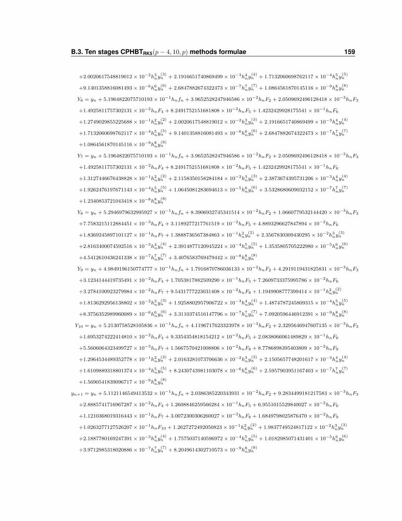
B.3. Ten stages CPHBTRK5(p− 4, 10, p) methods formulae 159
+2.0020617548819012× 10⁻²h3ny(3)n + 2.1916651740869499× 10⁻³h4ny
(4)n + 1.7132060698762117× 10⁻⁴h5ny
(5)n
+9.1401358816081493× 10⁻⁶h6ny(6)n + 2.6847882674322473× 10⁻⁷h7ny
(7)n + 1.0864561870145116× 10⁻⁹h8ny
(8)n
Y6 = yn + 5.1964822075710193× 10⁻¹hnfn + 3.9652528247946586× 10⁻²hnF2 + 2.0509692496128418× 10⁻³hnF3
+1.4925811757302131× 10⁻²hnF4 + 8.2491752151681808× 10⁻²hnF5 + 1.4232429928175541× 10⁻¹hnF6
+1.2749029855225688× 10⁻¹h2ny(2)n + 2.0020617548819012× 10⁻²h3ny
(3)n + 2.1916651740869499× 10⁻³h4ny
(4)n
+1.7132060698762117× 10⁻⁴h5ny(5)n + 9.1401358816081493× 10⁻⁶h6ny
(6)n + 2.6847882674322473× 10⁻⁷h7ny
(7)n
+1.0864561870145116× 10⁻⁹h8ny(8)n
Y7 = yn + 5.1964822075710193× 10⁻¹hnfn + 3.9652528247946586× 10⁻²hnF2 + 2.0509692496128418× 10⁻³hnF3
+1.4925811757302131× 10⁻²hnF4 + 8.2491752151681808× 10⁻²hnF5 + 1.4232429928175541× 10⁻¹hnF6
+1.3127446676438828× 10⁻¹h2ny(2)n + 2.1158350158284184× 10⁻²h3ny
(3)n + 2.3873674395731206× 10⁻³h4ny
(4)n
+1.9262476197671143× 10⁻⁴h5ny(5)n + 1.0645081283694613× 10⁻⁵h6ny
(6)n + 3.5328680609032152× 10⁻⁷h7ny
(7)n
+1.2340853721043418× 10⁻⁸h8ny(8)n
Y8 = yn + 5.2946979632995927× 10⁻¹hnfn + 8.3906932745341514× 10⁻²hnF2 + 1.0660779532144420× 10⁻³hnF3
+7.7583215112884451× 10⁻³hnF4 + 3.1189277217761519× 10⁻²hnF5 + 4.8893296627847894× 10⁻²hnF6
+1.8369245897101127× 10⁻¹hnF7 + 1.3888736567384863× 10⁻¹h2ny(2)n + 2.3567830309430295× 10⁻²h3ny
(3)n
+2.8163400074592516× 10⁻³h4ny(4)n + 2.3914877120945224× 10⁻⁴h5ny
(5)n + 1.3535805705222980× 10⁻⁵h6ny
(6)n
+4.5412610436241338× 10⁻⁷h7ny(7)n + 3.4076583769479442× 10⁻⁸h8ny
(8)n
Y9 = yn + 4.9849196150774777× 10⁻¹hnfn + 1.7916870786036133× 10⁻²hnF2 + 4.2919119431825831× 10⁻³hnF3
+3.1234144419735491× 10⁻²hnF4 + 1.7053817882509290× 10⁻¹hnF5 + 7.2609733375995786× 10⁻²hnF6
+3.2784100923279984× 10⁻²hnF7 + 9.5431777223031408× 10⁻²hnF8 + 1.1949908777399414× 10⁻¹h2ny(2)n
+1.8136292956138802× 10⁻²h3ny(3)n + 1.9258802957906722× 10⁻³h4ny
(4)n + 1.4874787245809315× 10⁻⁴h5ny
(5)n
+8.3756352989960089× 10⁻⁶h6ny(6)n + 3.3110374516147796× 10⁻⁷h7ny
(7)n + 7.0920596446912391× 10⁻⁹h8ny
(8)n
Y10 = yn + 5.2130758528105836× 10⁻¹hnfn + 4.1196717623323978× 10⁻³hnF2 + 2.3295646947607135× 10⁻³hnF3
+1.6953274222414810× 10⁻²hnF4 + 9.3354354818154212× 10⁻²hnF5 + 2.0838066061489829× 10⁻¹hnF6
+5.5606064323499727× 10⁻³hnF7 + 1.5667570421008806× 10⁻²hnF8 + 8.7786898395403809× 10⁻²hnF9
+1.2964534489352778× 10⁻¹h2ny(2)n + 2.0163281073706636× 10⁻²h3ny
(3)n + 2.1505657748201617× 10⁻³h4ny
(4)n
+1.6109889318801374× 10⁻⁴h5ny(5)n + 8.2430743981103078× 10⁻⁶h6ny
(6)n + 2.5957903951167403× 10⁻⁷h7ny
(7)n
+1.5690541839096717× 10⁻⁹h8ny(8)n
yn+1 = yn + 5.1121146549413532× 10⁻¹hnfn + 2.0386385220343931× 10⁻²hnF2 + 9.2834499181217583× 10⁻³hnF3
+2.8885741716967287× 10⁻²hnF4 + 1.2608846259566284× 10⁻¹hnF5 + 6.9551015529840027× 10⁻²hnF6
+1.1210368019316443× 10⁻¹hnF7 + 3.0072300306260027× 10⁻³hnF8 + 1.6849798025876470× 10⁻²hnF9
+1.0263277127526207× 10⁻¹hnF10 + 1.2627272492050823× 10⁻¹h2ny(2)n + 1.9837749524817122× 10⁻²h3ny
(3)n
+2.1887780169247391× 10⁻³h4ny(4)n + 1.7575037140596972× 10⁻⁴h5ny
(5)n + 1.0182985071431401× 10⁻⁵h6ny
(6)n
+3.9712985318020886× 10⁻⁷h7ny(7)n + 8.2049614302710573× 10⁻⁹h8ny
(8)n
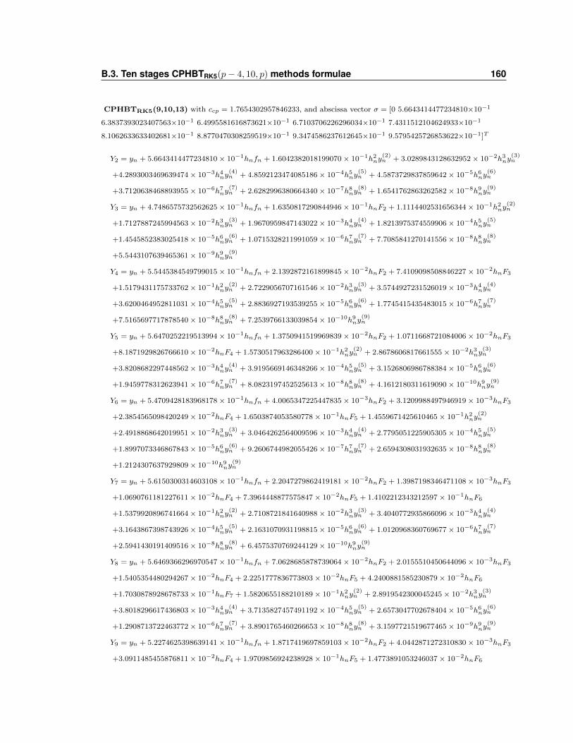
B.3. Ten stages CPHBTRK5(p− 4, 10, p) methods formulae 160
CPHBTRK5(9,10,13) with ccp = 1.7654302957846233, and abscissa vector σ = [0 5.6643414477234810×10⁻¹
6.3837393023407563×10⁻¹ 6.4995581616873621×10⁻¹ 6.7103706226296034×10⁻¹ 7.4311512104624933×10⁻¹
8.1062633633402681×10⁻¹ 8.8770470308259519×10⁻¹ 9.3474586237612645×10⁻¹ 9.5795425726853622×10⁻¹]T
Y2 = yn + 5.6643414477234810× 10⁻¹hnfn + 1.6042382018199070× 10⁻¹h2ny(2)n + 3.0289843128632952× 10⁻²h3ny
(3)n
+4.2893003469639474× 10⁻³h4ny(4)n + 4.8592123474085186× 10⁻⁴h5ny
(5)n + 4.5873729837859642× 10⁻⁵h6ny
(6)n
+3.7120638468893955× 10⁻⁶h7ny(7)n + 2.6282996380664340× 10⁻⁷h8ny
(8)n + 1.6541762863262582× 10⁻⁸h9ny
(9)n
Y3 = yn + 4.7486575732562625× 10⁻¹hnfn + 1.6350817290844946× 10⁻¹hnF2 + 1.1114402531656344× 10⁻¹h2ny(2)n
+1.7127887245994563× 10⁻²h3ny(3)n + 1.9670959847143022× 10⁻³h4ny
(4)n + 1.8213975374559906× 10⁻⁴h5ny
(5)n
+1.4545852383025418× 10⁻⁵h6ny(6)n + 1.0715328211991059× 10⁻⁶h7ny
(7)n + 7.7085841270141556× 10⁻⁸h8ny
(8)n
+5.5443107639465361× 10⁻⁹h9ny(9)n
Y4 = yn + 5.5445384549799015× 10⁻¹hnfn + 2.1392872161899845× 10⁻²hnF2 + 7.4109098508846227× 10⁻²hnF3
+1.5179431175733762× 10⁻¹h2ny(2)n + 2.7229056707161546× 10⁻²h3ny
(3)n + 3.5744927231526019× 10⁻³h4ny
(4)n
+3.6200464952811031× 10⁻⁴h5ny(5)n + 2.8836927193539255× 10⁻⁵h6ny
(6)n + 1.7745415435483015× 10⁻⁶h7ny
(7)n
+7.5165697717878540× 10⁻⁸h8ny(8)n + 7.2539766133039854× 10⁻¹⁰h9ny
(9)n
Y5 = yn + 5.6470252219513994× 10⁻¹hnfn + 1.3750941519969839× 10⁻²hnF2 + 1.0711668721084006× 10⁻²hnF3
+8.1871929826766610× 10⁻²hnF4 + 1.5730517963286400× 10⁻¹h2ny(2)n + 2.8678606817661555× 10⁻²h3ny
(3)n
+3.8208682297448562× 10⁻³h4ny(4)n + 3.9195669146348266× 10⁻⁴h5ny
(5)n + 3.1526806986788384× 10⁻⁵h6ny
(6)n
+1.9459778312623941× 10⁻⁶h7ny(7)n + 8.0823197452525613× 10⁻⁸h8ny
(8)n + 4.1612180311619090× 10⁻¹⁰h9ny
(9)n
Y6 = yn + 5.4709428183968178× 10⁻¹hnfn + 4.0065347225447835× 10⁻³hnF2 + 3.1209988497946919× 10⁻³hnF3
+2.3854565098420249× 10⁻²hnF4 + 1.6503874053580778× 10⁻¹hnF5 + 1.4559671425610465× 10⁻¹h2ny(2)n
+2.4918868642019951× 10⁻²h3ny(3)n + 3.0464262564009596× 10⁻³h4ny
(4)n + 2.7795051225905305× 10⁻⁴h5ny
(5)n
+1.8997073346867843× 10⁻⁵h6ny(6)n + 9.2606744982055426× 10⁻⁷h7ny
(7)n + 2.6594308031932635× 10⁻⁸h8ny
(8)n
+1.2124307637929809× 10⁻¹⁰h9ny(9)n
Y7 = yn + 5.6150300314603108× 10⁻¹hnfn + 2.2047279862419181× 10⁻²hnF2 + 1.3987198346471108× 10⁻³hnF3
+1.0690761181227611× 10⁻²hnF4 + 7.3964448877575847× 10⁻²hnF5 + 1.4102212343212597× 10⁻¹hnF6
+1.5379920896741664× 10⁻¹h2ny(2)n + 2.7108721841640988× 10⁻²h3ny
(3)n + 3.4040772935866096× 10⁻³h4ny
(4)n
+3.1643867398743926× 10⁻⁴h5ny(5)n + 2.1631070931198815× 10⁻⁵h6ny
(6)n + 1.0120968360769677× 10⁻⁶h7ny
(7)n
+2.5941430191409516× 10⁻⁸h8ny(8)n + 6.4575370769244129× 10⁻¹⁰h9ny
(9)n
Y8 = yn + 5.6469366296970547× 10⁻¹hnfn + 7.0628685878739064× 10⁻²hnF2 + 2.0155510450644096× 10⁻³hnF3
+1.5405354480294267× 10⁻²hnF4 + 2.2251777836773803× 10⁻²hnF5 + 4.2400881585230879× 10⁻²hnF6
+1.7030878928678733× 10⁻¹hnF7 + 1.5820655188210189× 10⁻¹h2ny(2)n + 2.8919542300045245× 10⁻²h3ny
(3)n
+3.8018296617436803× 10⁻³h4ny(4)n + 3.7135827457491192× 10⁻⁴h5ny
(5)n + 2.6573047702678404× 10⁻⁵h6ny
(6)n
+1.2908713722463772× 10⁻⁶h7ny(7)n + 3.8901765460266653× 10⁻⁸h8ny
(8)n + 3.1597721519677465× 10⁻⁹h9ny
(9)n
Y9 = yn + 5.2274625398639141× 10⁻¹hnfn + 1.8717419697859103× 10⁻²hnF2 + 4.0442871272310830× 10⁻³hnF3
+3.0911485455876811× 10⁻²hnF4 + 1.9709856924238928× 10⁻¹hnF5 + 1.4773891053246037× 10⁻²hnF6
B.3. Ten stages CPHBTRK5(p− 4, 10, p) methods formulae 161
+3.3854950950856257× 10⁻²hnF7 + 1.1259900486227652× 10⁻¹hnF8 + 1.3296233301514793× 10⁻¹h2ny(2)n
+2.1822926715599468× 10⁻²h3ny(3)n + 2.5833852769707099× 10⁻³h4ny
(4)n + 2.3334707362756188× 10⁻⁴h5ny
(5)n
+1.6544350421996948× 10⁻⁵h6ny(6)n + 9.2256266420882364× 10⁻⁷h7ny
(7)n + 3.8114058091853727× 10⁻⁸h8ny
(8)n
+7.6966328682629719× 10⁻¹⁰h9ny(9)n
Y10 = yn + 5.5531192978880639× 10⁻¹hnfn + 5.3764637578485371× 10⁻³hnF2 + 1.5631810589904864× 10⁻³hnF3
+1.1947778940949956× 10⁻²hnF4 + 8.0570920327995371× 10⁻²hnF5 + 1.6731364385117536× 10⁻¹hnF6
+5.1202385489403604× 10⁻²hnF7 + 1.4039855599479078× 10⁻²hnF8 + 7.0628098453887372× 10⁻²hnF9
+1.4864140122137892× 10⁻¹h2ny(2)n + 2.5263114945332763× 10⁻²h3ny
(3)n + 3.0139230915772709× 10⁻³h4ny
(4)n
+2.6220053893687010× 10⁻⁴h5ny(5)n + 1.6620242481144206× 10⁻⁵h6ny
(6)n + 7.3826610214186177× 10⁻⁷h7ny
(7)n
+2.1078596933910890× 10⁻⁸h8ny(8)n + 1.8626100464508011× 10⁻¹⁰h9ny
(9)n
yn+1 = yn + 5.4549943335143936× 10⁻¹hnfn + 1.6044307468663078× 10⁻²hnF2 + 1.1112257019290070× 10⁻²hnF3
+1.7048730209331123× 10⁻²hnF4 + 1.1759027601172016× 10⁻¹hnF5 + 6.3764920206474354× 10⁻²hnF6
+1.1616987855667295× 10⁻¹hnF7 + 2.4316881895940735× 10⁻³hnF8 + 1.2232712198989968× 10⁻²hnF9
+9.8105796787824953× 10⁻²hnF10 + 1.4470082321380714× 10⁻¹h2ny(2)n + 2.4660993945625851× 10⁻²h3ny
(3)n
+2.9995764659038575× 10⁻³h4ny(4)n + 2.7265581508943048× 10⁻⁴h5ny
(5)n + 1.8745611941477079× 10⁻⁵h6ny
(6)n
+9.5451738579298906× 10⁻⁷h7ny(7)n + 3.3330769972075675× 10⁻⁸h8ny
(8)n + 6.2522836798074345× 10⁻¹⁰h9ny
(9)n
CPHBTRK5(10,10,14) with ccp = 1.6845263293032087, and abscissa vector σ = [0 5.9343005761842926×10⁻¹
6.6032312085122502×10⁻¹ 6.7035766911908345×10⁻¹ 6.9757269007435319×10⁻¹ 7.6612963307130821×10⁻¹
8.2552005004722695×10⁻¹ 8.9691172353251647×10⁻¹ 9.3998752728239798×10⁻¹ 9.6102884854375048×10⁻¹]T
Y2 = yn + 5.9343005761842926× 10⁻¹hnfn + 1.7607961664250613× 10⁻¹h2ny(2)n + 3.4830312349864452× 10⁻²h3ny
(3)n
+5.1673385661619876× 10⁻³h4ny(4)n + 6.1329080461028796× 10⁻⁴h5ny
(5)n + 6.0657532919456007× 10⁻⁵h6ny
(6)n
+5.1422861793406494× 10⁻⁶h7ny(7)n + 3.8144839796207175× 10⁻⁷h8ny
(8)n + 2.5151438309009976× 10⁻⁸h9ny
(9)n
+1.4925619484902157× 10⁻⁹h10n y(10)n
Y3 = yn + 5.0535595019487956× 10⁻¹hnfn + 1.5496717065634544× 10⁻¹hnF2 + 1.2605113495379075× 10⁻¹h2ny(2)n
+2.0699850180014245× 10⁻²h3ny(3)n + 2.5240790744149640× 10⁻³h4ny
(4)n + 2.4539978387501469× 10⁻⁴h5ny
(5)n
+2.0094837324664023× 10⁻⁵h6ny(6)n + 1.4609531725622789× 10⁻⁶h7ny
(7)n + 9.9575684975054986× 10⁻⁸h8ny
(8)n
+6.6606958767845225× 10⁻⁹h9ny(9)n + 4.4547456036785224× 10⁻¹⁰h10n y
(10)n
Y4 = yn + 5.8322457938957528× 10⁻¹hnfn + 1.8037219764057973× 10⁻²hnF2 + 6.9095869965450099× 10⁻²hnF3
+1.6836027341600762× 10⁻¹h2ny(2)n + 3.1967682168035506× 10⁻²h3ny
(3)n + 4.4703389616453110× 10⁻³h4ny
(4)n
+4.8755394490671526× 10⁻⁴h5ny(5)n + 4.2691671444262734× 10⁻⁵h6ny
(6)n + 3.0207989079127973× 10⁻⁶h7ny
(7)n
+1.6822693206402487× 10⁻⁷h8ny(8)n + 6.5128616296313862× 10⁻⁹h9ny
(9)n + 5.1850482333369511× 10⁻¹¹h10n y
(10)n
Y5 = yn + 5.9208869215473492× 10⁻¹hnfn + 6.9403773956583162× 10⁻³hnF2 + 1.0274033710763762× 10⁻²hnF3
+8.8269586813196299× 10⁻²hnF4 + 1.7322882393716457× 10⁻¹h2ny(2)n + 3.3278833204487601× 10⁻²h3ny
(3)n
+4.6995817706428156× 10⁻³h4ny(4)n + 5.1649571436544371× 10⁻⁴h5ny
(5)n + 4.5448390433200733× 10⁻⁵h6ny
(6)n
+3.2182676339911780× 10⁻⁶h7ny(7)n + 1.7786896769317757× 10⁻⁷h8ny
(8)n + 6.6455794310577777× 10⁻⁹h9ny
(9)n
B.3. Ten stages CPHBTRK5(p− 4, 10, p) methods formulae 162
+1.8416446761273598× 10⁻¹¹h10n y(10)n
Y6 = yn + 5.7841507532521941× 10⁻¹hnfn + 1.8634924880678789× 10⁻³hnF2 + 2.7585797645732213× 10⁻³hnF3
+2.3700398778623545× 10⁻²hnF4 + 1.5939208671482422× 10⁻¹hnF5 + 1.6347459009250773× 10⁻¹h2ny(2)n
+2.9911749890355704× 10⁻²h3ny(3)n + 3.9501502209028268× 10⁻³h4ny
(4)n + 3.9604582544246685× 10⁻⁴h5ny
(5)n
+3.0690725796041343× 10⁻⁵h6ny(6)n + 1.8131663928410011× 10⁻⁶h7ny
(7)n + 7.6191053016103847× 10⁻⁸h8ny
(8)n
+1.7843501303036769× 10⁻⁹h9ny(9)n + 4.9448190264126259× 10⁻¹²h10n y
(10)n
Y7 = yn + 5.9043043232493331× 10⁻¹hnfn + 1.7958730528799361× 10⁻²hnF2 + 1.4586072801606044× 10⁻³hnF3
+1.2531656559352036× 10⁻²hnF4 + 8.3581028538824861× 10⁻²hnF5 + 1.1955959481515684× 10⁻¹hnF6
+1.7081859040696901× 10⁻¹h2ny(2)n + 3.2043520019335005× 10⁻²h3ny
(3)n + 4.3369550953010101× 10⁻³h4ny
(4)n
+4.4422177001322740× 10⁻⁴h5ny(5)n + 3.4876686890540442× 10⁻⁵h6ny
(6)n + 2.0486024982127579× 10⁻⁶h7ny
(7)n
+8.1869942644563346× 10⁻⁸h8ny(8)n + 1.6561472495679913× 10⁻⁹h9ny
(9)n + 4.5290135142888129× 10⁻¹¹h10n y
(10)n
Y8 = yn + 5.8900894046938557× 10⁻¹hnfn + 8.6657695471225551× 10⁻²hnF2 + 3.9802886706887414× 10⁻⁴hnF3
+3.4196737741949992× 10⁻³hnF4 + 2.2807826719538012× 10⁻²hnF5 + 3.2625759324504865× 10⁻²hnF6
+1.6199379890659854× 10⁻¹hnF7 + 1.7360999944418690× 10⁻¹h2ny(2)n + 3.3817549911252742× 10⁻²h3ny
(3)n
+4.8305235381998508× 10⁻³h4ny(4)n + 5.2911112323407179× 10⁻⁴h5ny
(5)n + 4.4915956888063516× 10⁻⁵h6ny
(6)n
+2.8892171954995373× 10⁻⁶h7ny(7)n + 1.3114966443703605× 10⁻⁷h8ny
(8)n + 3.9158387856764826× 10⁻⁹h9ny
(9)n
+2.5778593577831624× 10⁻¹⁰h10n y(10)n
Y9 = yn + 5.5631602197664731× 10⁻¹hnfn + 1.7211673796407412× 10⁻²hnF2 + 3.2004516719069138× 10⁻³hnF3
+2.7496750998476687× 10⁻²hnF4 + 1.8488586449448124× 10⁻¹hnF5 + 1.9238705072271198× 10⁻²hnF6
+2.8220794727845982× 10⁻²hnF7 + 1.0341726454436123× 10⁻¹hnF8 + 1.5126470023518393× 10⁻¹h2ny(2)n
+2.6675948167045008× 10⁻²h3ny(3)n + 3.4118853719250276× 10⁻³h4ny
(4)n + 3.3487074568373207× 10⁻⁴h5ny
(5)n
+2.5965582862179711× 10⁻⁵h6ny(6)n + 1.6047369990862359× 10⁻⁶h7ny
(7)n + 7.7702807418301099× 10⁻⁸h8ny
(8)n
+2.7290451952662450× 10⁻⁹h9ny(9)n + 5.0521164706530579× 10⁻¹¹h10n y
(10)n
Y10 = yn + 5.8532833450920740× 10⁻¹hnfn + 4.0529692379392655× 10⁻³hnF2 + 2.7535633275909705× 10⁻³hnF3
+2.3657299949851572× 10⁻²hnF4 + 6.6773909399830647× 10⁻²hnF5 + 1.5682791565300769× 10⁻¹hnF6
+4.5278658792413586× 10⁻²hnF7 + 1.1328429325961174× 10⁻²hnF8 + 6.5027768347948267× 10⁻²hnF9
+1.6631147411677050× 10⁻¹h2ny(2)n + 3.0315896169288176× 10⁻²h3ny
(3)n + 3.9396077751724448× 10⁻³h4ny
(4)n
+3.8244988042746535× 10⁻⁴h5ny(5)n + 2.8128828547723106× 10⁻⁵h6ny
(6)n + 1.5466195375570637× 10⁻⁶h7ny
(7)n
+6.0872653315290231× 10⁻⁸h8ny(8)n + 1.5906008354109543× 10⁻⁹h9ny
(9)n + 1.1210073202001079× 10⁻¹¹h10n y
(10)n
yn+1 = yn + 5.7477438181988205× 10⁻¹hnfn + 1.2723618159852982× 10⁻²hnF2 + 1.3564521219555059× 10⁻²hnF3
+1.9218057567157325× 10⁻²hnF4 + 1.1485428369921558× 10⁻¹hnF5 + 5.4975225293228937× 10⁻²hnF6
+1.0629387862938201× 10⁻¹hnF7 + 1.7516258263226465× 10⁻³hnF8 + 1.0054731789283433× 10⁻²hnF9
+9.1789675996120271× 10⁻²hnF10 + 1.6138949160591556× 10⁻¹h2ny(2)n + 2.9319726209364978× 10⁻²h3ny
(3)n
+3.8422803320804179× 10⁻³h4ny(4)n + 3.8258855495751858× 10⁻⁴h5ny
(5)n + 2.9602804594150724× 10⁻⁵h6ny
(6)n
+1.7789840626988628× 10⁻⁶h7ny(7)n + 8.0703132790948057× 10⁻⁸h8ny
(8)n + 2.5468406137515121× 10⁻⁹h9ny
(9)n

B.3. Ten stages CPHBTRK5(p− 4, 10, p) methods formulae 163
+4.3658347039740745× 10⁻¹¹h10n y(10)n
Bibliography
[1] Arenstorf, R. F. Periodic solutions of the restricted three body problem repre-
senting analytic continuations of Keplerian elliptic motions. American Journal
of Mathematics, 27-35 (1963).
[2] Barrio, R. Performance of the Taylor series method for ODEs/DAEs. Appl.
Math. Comput.,163, pp. 525–545 (2005).
[3] Barrio, R., Blesa, F., and Lara, M. VSVO formulation of the Taylor method for
the numerical solution of ODEs. Computers and Mathematics with Applications,
50(1), 93-111 (2005).
[4] Binney, J. and Tremaine, S. Galactic dynamics. Princeton university press
(2011).
[5] Bozic, V. Three-stage Hermite-Birkhoff-Taylor Ode Solver with a C++ Program.
Thesis, University of Ottawa (2008).
[6] Butcher, J. C. Numerical methods for ordinary differential equations. Wiley
(2008).
[7] Butcher, J. C. The numerical analysis of ordinary differential equations: Runge-
Kutta and general linear methods. Wiley-Interscience (1987).
[8] Corliss, G. F. and Chang, Y. F. Solving ordinary differential equations using
Taylor series. ACM Trans. Math. Software 8:114–144 (1982).
164
BIBLIOGRAPHY 165
[9] Daniel, J. W. and Moore, R. E. Computation and theory in ordinary differential
equations. W. H. Freeman, San Francisco (1970).
[10] Davis, H. T. Introduction to nonlinear differential and integral equations. Courier
Dover Publications (1962).
[11] Deprit, A. and Zahar, R. M. W., Numerical integration of an orbit and its con-
comitant variations. Z. Angew. Math. Phys. 17:425–430 (1966).
[12] Dormand, J. R., El-Mikkawy, M. E. A. and Prince, P. J. Families of Runge-Kutta-
Nystrom formulae. IMA Journal of Numerical Analysis, 7(2), 235-250 (1987).
[13] Dormand, J. R. and Prince, P. New Runge-Kutta algorithms for numerical sim-
ulation in dynamical astronomy. Celestial Mechanics, 18(3), 223-232 (1978).
[14] Duncan, M., Quinn, T. and Tremaine, S. The long-term evolution of orbits in
the Solar System: A mapping approach. Icarus, 82(2), 402-418 (1989).
[15] Fehlberg, E. Classical eight- and lower-order Runge-Kutta-Nystrom formulas
with step-size control for special second-order differential equations. NASA TRR-
381 (1972).
[16] Frost, A. and Pearson, R. Kinetics and mechanism. The Journal of Physical
Chemistry, 65(2), 384-384 (1961).
[17] Gottlieb, S., and Gottlieb, L. A. J. Strong stability preserving properties of
Runge-Kutta time discretization methods for linear constant coefficient opera-
tors. Journal of Scientific Computing, 18(1), 83-109 (2003).
[18] Gottlieb, S., Ketcheson, D. I. and Shu, C. W. Strong stability preserving Runge-
Kutta and multistep time discretizations. Singapore: World Scientific (2011).
[19] Gottlieb, S., Ketcheson, D. I. and Shu, C. W. High order strong stability preserv-
ing time discretizations. Journal of Scientific Computing, 38(3), 251-289 (2009).
BIBLIOGRAPHY 166
[20] Gottlieb, S., and Shu, C. W. Total variation diminishing Runge-Kutta schemes.
Mathematics of Computation of the American Mathematical Society, 67(221),
73-85 (1998).
[21] Gottlieb, S., Shu, C. W. and Tadmor, E. Strong stability-preserving high-order
time discretization methods. SIAM review, 43(1), 89-112 (2001).
[22] Hairer, E., Nørsett, S. P. and Wanner G. Solving ordinary differential equations
I: Nonstiff problems. Springer, 2000.
[23] Hairer, E. and Wanner, G. Solving ordinary differential equations II. volume 14
of Springer Series in Computational Mathematics (1991).
[24] Henon, M. and Heiles, C. The applicability of the third integral of motion: some
numerical experiments. The Astronomical Journal, 69, 73 (1964).
[25] Hoefkens, J., Berz, M. and Makino, K. Computing validated solutions of implicit
differential equations. Adv. Comput. Math. 19:231–253 (2003).
[26] Huang, C. Strong stability preserving hybrid methods. Applied Numerical Math-
ematics, 59(5), 891-904 (2009).
[27] Hull, T. E., Enright, W. H., Fellen, B. M. and Sedgwick, A. E. Comparing nu-
merical methods for ordinary differential equations. SIAM Journal on Numerical
Analysis, 9(4), 603-637 (1972).
[28] Hundsdorfer, W., Ruuth, S. J., and Spiteri, R. J. Monotonicity-preserving linear
multistep methods. SIAM Journal on Numerical Analysis, 41(2), 605-623 (2003).
[29] Jorba, A. and Zou, M. A software package for the numerical integration of ODEs
by means of high-order Taylor methods. Experimental Mathematics 14(1), 99-117
(2005).
BIBLIOGRAPHY 167
[30] Ketcheson, D. I. Highly efficient strong stability-preserving Runge-Kutta methods
with low-storage implementations. SIAM Journal on Scientific Computing, 30(4),
2113-2136 (2008).
[31] Kraaijevanger, J. F. B. M. Contractivity of Runge-Kutta methods. BIT Numerical
Mathematics, 31(3), 482-528 (1991).
[32] Krogh, F. T. VODQ, SVDQ, DVDQ: Variable order integrators for the numerical
solution of ordinary differential equations.. Jet Propulsion Laboratory, Calif. Inst.
of Technology (1970).
[33] Lambert, J. D. Numerical methods for ordinary differential systems: the initial
value problem. John Wiley and Sons, Inc. (1991).
[34] Lara, M., Elipe, A. and Palacios, M. Automatic programming of recurrent power
series. Mathematics and computers in Simulation, 49(4), 351-362 (1999).
[35] Li, G. Generation of Rooted Trees and Free Trees. Thesis, University of Victoria
(1996).
[36] Li, Y. Variable-step Variable-order 3-stage Hermite-Birkhoff Ode Solver of Order
5 to 15 with A C++ Program. University of Ottawa (2008).
[37] Moore, R. E. Interval analysis. Prentice-Hall Englewood Cliffs (1966).
[38] Nedialkov, N. S., Jackson, K. R. and Corliss, G. F. Validated solutions of initial
value problems for ordinary differential equations. Appl. Math. Comput. 105:21–
68 (1999).
[39] Newton, I. Methodus Fluxionum 1671. Mathematical Papers (2nd ed.), Vol. III
Cambridge Univ. Press, Cambridge (1967-1981).
BIBLIOGRAPHY 168
[40] Nguyen-Ba, T., Desjardins, S. J., Sharp, P. W. and Vaillancourt, R.
Contractivity-preserving explicit Hermite-Obrechkoff ODE solver of order 13. Ce-
lestial Mechanics and Dynamical Astronomy, 117(4), 423-434 (2013).
[41] Nguyen-Ba, T., Hao, H., Yagoub, H. and Vaillancourt, R. One-step 5-stage
Hermite-Birkhoff-Taylor ODE solver of order 12. Applied Mathematics and
Computation, 211(2), 313-328 (2009).
[42] Nguyen-Ba, T., Karouma, A., Giordano, T. and Vaillancourt, R. Strong-stability-
preserving, One-step, 9-stage, Hermite–Birkhoff–Taylor, Time discretization
Methods Combining Taylor and RK4 Methods. Boundary Field Problems and
Computer Simulation (2012).
[43] Prince, P. J. and Dormand, J. R. High order embedded Runge-Kutta formulae.
Journal of Computational and Applied Mathematics, 7(1), 67-75 (1981).
[44] Reich, S. Preservation of adiabatic invariants under symplectic discretization.
Applied numerical mathematics, 29(1), 45-55 (1999).
[45] Ruuth, S. Global optimization of explicit strong-stability-preserving Runge-Kutta
methods. Mathematics of Computation, 75(253), 183-207 (2006).
[46] Ruuth, S. J. , Spiteri, R. J. Two barriers on strong-stability-preserving time
discretization methods. J. Sci. Comput. 17, 211–220 (2002).
[47] Ruuth, S. J., and Spiteri, R. J. High-order strong-stability-preserving Runge-
Kutta methods with downwind-biased spatial discretizations. SIAM Journal on
Numerical Analysis, 42(3), 974-996 (2004).
[48] Shampine, L. F. and Gordon, M. K. Computer Solution of Ordinary Differential
Equations: The Initial Value Problem. Freeman, San Francisco (1975).
BIBLIOGRAPHY 169
[49] Sharp, P. W., Qureshi, M. A. and Grazier, K. R. High order explicit Runge-
Kutta-Nystrom pairs. Numerical Algorithms, 62(1), 133-148 (2013).
[50] Sharp, P. W. N-body simulations: The performance of some integrators. ACM
Transactions on Mathematical Software (TOMS), 32(3), 375-395 (2006).
[51] Sharp, P. W. Numerical comparisons of some explicit Runge-Kutta pairs of orders
4 through 8. ACM Transactions on Mathematical Software (TOMS), 17(3), 387-
409 (1991).
[52] Shu, C. W. Total-variation-diminishing time discretizations. SIAM Journal on
Scientific and Statistical Computing, 9(6), 1073-1084 (1988).
[53] Shu, C. W. and Osher, S. Efficient implementation of essentially non-oscillatory
shock-capturing schemes. Journal of Computational Physics, 77(2), 439-471
(1988).
[54] Spiteri, R. J., and Ruuth, S. J. Non-linear evolution using optimal fourth-order
strong-stability-preserving Runge-Kutta methods. Mathematics and Computers
in Simulation, 62(1), 125-135 (2003).
[55] Spiteri, R. J. and Ruuth, S. J. A new class of optimal high-order strong-stability-
preserving time-stepping schemes. SIAM J. Numer. Anal. 40,469–491 (2007).
[56] Spiteri, R. J. and Ruuth, S. J. A new class of optimal high-order strong-stability-
preserving time discretization methods. SIAM Journal on Numerical Analysis,
40(2), 469-491 (2002).
[57] Steffensen, J. F. On the restricted problem of three bodies. Mat.-fys. medd.; Bd
30 (1956).
[58] Szebehely, V. Theory of orbits. The restricted problem of three bodies. New York:
Academic Press, c1967, 1 (1967).

![PLANETARY BIRKHOFF NORMAL FORMS · PLANETARY BIRKHOFF NORMAL FORMS 625 below. On the reduced phase spaces, one can construct Birkhoff normal forms ([6, Sect 7 and 9]; §2, §5.1below)](https://img.dokumen.tips/doc/110x75/6047d6bd37fe306c735bee69/planetary-birkhoff-normal-planetary-birkhoff-normal-forms-625-below-on-the-reduced.jpg)