On Hermite-Birkhoff Interpolation*ON HERMITE-BIRKHOFF INTERPOLATION 95 Using a determinantal formulation of the problem, which is essential in this context, and arguments on the number

JOURNAL OF APPROXIMATION THEORY 6, 90-114 (1972)

On Hermite-Birkhoff Interpolation*

SAMUEL KARLIN+ AND JOHN M. KARON*

Department of’ Mathematics, Colorado College, Colorado Springs, Colorado 80903

Received December 18, 1970

DEDICATED TO PROFESSOR J. L. WALSH ON THE OCCASION OF HIS 75TH BIRTHDAY

In recent years there has been renewed interest and progress on Hermite- Birkhoff (HB) interpolation. The original source for this activity is work by G. D. Birkhoff in 1906 [3], with a notable contribution by G. P6lya in 1931 [15]. The concrete formulation of the problem is: Given n ordered pairs (i,j), 1 < i < k, 0 < j d n - 1, with Z designating the set of such ordered pairs, and n numbers f :j’, under what conditions on the interpolation points {xi}: and the set Z is it possible to determine a unique polynomial p(x) E “n-1 , the class of polynomials of degree at most n - 1, satisfying

p’qx.) = p I z when (i, ,j) E Z ?

Various restrictions are placed on the xi . For example, we may require that all are real, or more specifically x1 < x2 < ... -=c xk . Problems for which interpolation is unique for all appropriate choices of the points are called poised.

The customary formulation of HB interpolation problems in terms of an incidence matrix is done in Section 1, and the known results on HB polynomial interpolation problems are reviewed in Section 2. Section 3 presents three new theorems on nonpoised problems, highlighting an important perturbation technique. Sketches of the proofs are included. An example of a poised problem specifying linear combinations of derivatives is set forth in Section 4. The problem of HB interpolation by polynomial splines

* Research supported in part by NSF grant G 7110 and ONR NGOO-14-67-A-0112- 0015 at Stanford University.

t Department of Mathematics, Stanford University, Stanford, CA and Weizmann Institute of Science, Rehovot, Israel.

r Departments of Mathematics, Stanford University, Stanford, CA and Syracuse University, Syracuse, NY.

90 Copyright 0 1972 by Academic Press, Inc. All rights of reproduction in any form reserved.

ON HERMITE-BIRKHOFF INTERPOLATION 91

seems innately more complex; some results are indicated in Section 5. Several open problems are listed in the concluding section.

It is worthwhile to emphasize that the results announced in this paper persist for polynomials induced by extended-complete-Tchebycheff systems (ECT systems) and T-splines, as well as ordinary polynomials and polynomial splines.

ADDED IN PROOF: A. Sharma [23] has also reviewed the current knowledge of Hermite-Birkhoff interpolation. The last half of his paper reviews the work of Turan and his school, and applications to expansions, quadrature, and completely convex functions. The first part includes sketches of proofs of known results on HB interpolation, and a result explaining the difference between our examples in (2.5) and (2.7).

In addition, Micchelli and Rivlin [24] recently studied quadrature formulae corresponding to HB incidence matrices.

1. FORMULATIONS OF THE PROBLEM

Schoenberg [17] stated the HB polynomial interpolation problem in terms of a k x II incidence matrix E = 11 eii /I, where

IL (&A E4 ‘ii = 10, otherwise.

Here E exhibits n entries equal to 1, corresponding to the interpolation conditions, and all other entries of value 0. We can obviously stipulate that each row of E contains at least one 1.

Since the problem is linear and we are interested in unicity, without loss of generality we can assume that all flj’ = 0 in Eq. (0.1). A polynomial p(x) E rrsel fulfilling the homogeneous interpolation conditions is said to interpolate E with zero data.

The incidence matrix is called poised with respect to {xi>: if the only polynomial interpolating E at {Xi): with zero data is the trivial polynomial. E is called unconditionally poised if it is poised with respect to all choices {xi): and order-poised if it is poised with respect to all real choices of k points with the ordering x, < x8 < ..* < xk .

By a shift of the origin and a change of scale, we may suppose without restricting generality that x1 = 0, xk = 1, and 0 < Xi < 1, 1 < i < k. With this convention, an equivalent statement of the problem is: Does there exist {xi};-‘, 0 < x2 < xs < ... < x~-~ < 1, such that

92 KARLIN AND KARON

where, in the case of polynomial interpolation U&V) = xl-l; in the more general case of an ECT system, the uz(x) are defined explicitly as in [7, p. 2761 and form a basis of solutions for a suitable n-th order differential equation.

Each interpolation condition generates one row of the determinant, and Dj is the j-th composed derivative operator. For example, the problem

P(O) = P(l) = 0

P’k? = P”(5) = 0, O<f<l,

corresponds to the incidence matrix

II 0 1 1000 0 1 0 1 0 0 II and the associated determinant is

100 0 0 1 25 352 0 0 2 65 1111

Ferguson [5] in establishing Theorem III, below, involving complex interpolation points dealt directly with a corresponding determinantal formula. Proofs of all other known results have relied decisively on appropriate variants of Rolle’s theorem and induction procedures. Our methods work primarily with the determinant (1.1) and exploit some cases of the determinantal inequalities related to total positivity developed in Karlin [7, Chap. lo].

2. REVIEW OF KNOWN RESULTS

In 1931, Polya [15] laid the foundation for much of the later work by effectively applying Rolle’s theorem in the analysis of two-point HB interpolation problems with x1 and x, real. He underscored the relevance of certain conditions on the incidence matrix, since commonly called the Pdlya conditions (see (2.2)). Let the incidence matrix be E = ]I eif [IF1 , Tz, and define

mj = C eij , i=l

(2.1)

Mj = c m, . “4


Thus, if p(x) interpolates E with zero data, mj is the number of requirements on the j-th derivative, and Mj , the number of requirements on the polynomial up to and including its j-th derivative.

THEOREM I. (Polya [15]). Let k = 2. E is poised zj” and only if the Pdlya conditions

prevail.

Mj >j+ 1, j = 0, I,..., n - 1, (2.2)

Since Polya’s line of analysis has been principally followed in establishing the results summarized in this section, we will review his arguments. An appropriate application of Rolle’s theorem implies that for any polynomial p(x) E rrnel interpolating E, p(j)(x) admits at least iVj - j zeros on [x1 , x2]. Therefore, if (2.2) holds, p(j)(x) has at least one zero. In particular, p(+l)(x) = 0. Proceeding backward we infer that p(x) = 0, and so E is poised. Suppose, conversely, that (2.2) is invalid and therefore for some Y, A& < v. Then there are more variables than conditions for the induced interpolation problem for p(“)(x) and consequently there exists a nontrivial polynomial of degree at most v interpolating E.

COROLLARY. Let E be an n-incidence matrix which does not satisfy the Pdlya conditions. Then E is not poised with respect to any set of points.

It is noteworthy that Polya was led to consider the interpolation problem through investigations concerning thin, curved, homogeneous beams, with given displacement, slope, moment, and/or shearing force prescribed at one or both ends. He wished to ascertain what combinations of four boundary conditions imply that the corresponding differential equation possesses a unique solution. More general Hermite-Birkhoff interpolation problems, involving k points, characterize special solutions of certain differential equations involving forcing functions at interior points. Corresponding results for ECT-systems are needed for the characterization of solutions for general differential equations. In this connection, see Karlin [7, Chap. 10, p. 5341.

Schoenberg revitalized the subject of HB interpolation in 1966 through his studies of HB interpolation problems with k 3 2 points. The conditions at x = xi are called Hermite if they comprise only interpolation of consecutive derivatives, commencing with the value of the function itself. E is called an Hermite matrix if it contains exclusively Hermite data, and quasi Hermite if it embraces only Hermite data except at the endpoints x1 and xk .

We record the following simple result. The proof can be found in Davis ~4, P. 291.

94 KARLIN AND KARON

PROPOSITION I. An Hermite matrix is unconditionally poised.

Concerning quasi Hermite matrices, we have

THEOREM II (Schoenberg [17]). Let E be a quasi-Hermite matrix, and let all interpolation points (xi>: be real. Then E is order-poised ij” and only if the Polya conditions (2.2) are satisfied.

Remark. The Polya conditions hold trivially if E is an Hermite matrix. Furthermore, a quasi-Hermite matrix satisfying the Polya conditions remains poised if the interior interpolation nodes x2 , x3 ,..., xLmI are reordered or altered but remain in the interval (x1 , xk).

Ferguson and, independently, Atkinson and Sharma advanced the theory of HB interpolation problems by making the elementary but relevant obser- vation that some incidence matrices can be decomposed into problems of lower degree. We state this fact formally in the following proposition:

PROPOSITION II. (Ferguson [5], Atkinson and Sharma [2]). Suppose that some Pdlya constant M,, for the incidence matrix E (see (2.1)) satisfies

l%&,=v+1. (2.3)

Then columns 0, I,..., v of E constitute an v + 1 incidence matrix E,; columns v + 1, v + 2,..., n - 1 comprise an n - v - 1 incidence matrix E,; and E is poised at {xi}: if and only if both E1 and E, are poised with respect to these points.

Designate such a decomposition by E = E1 @ E, . Note that we must allow E1 and ES to contain rows composed entirely of zeros. For example, the incidence matrix

Ii

1100010 0011010 0100000 II

can be decomposed into

and it follows from Propositions I and II and Theorem IV that the problem is unconditionally poised.

By virtue of Proposition II it suffices to consider only n-incidence matrices satisfying the strong Polya conditions

Mj tj+2, j = 0, l,..., n - 2. (2.4)

Ferguson examined HB interpolation with complex interpolation points.


Using a determinantal formulation of the problem, which is essential in this context, and arguments on the number of zeros of a polynomial he established the following striking result. We shall provide a simpler proof in [9].

THEOREM III (Ferguson [5]). An incidence matrix E satisfying the strong Pdlya conditions is unconditionally poised for complex interpolation points tf and only tf k = 2, or else E is an Hermite matrix.

Ferguson and, independently, Atkinson and Sharma noted the important fact that even blocks in the incidence matrix-i.e., the prescription of an even number of consecutive derivatives not starting with the 0-th-do not interfere with the application of Rolle’s theorem, since there must be an odd number of zeros off’(x) between consecutive zeros off(x).

THEOREM IV (Ferguson [5]; Atkinson and Sharma [2]). An incidence matrix E satisfying the Pdlya conditions is unconditionally poised for real points provided E contains only Hermite data and even blocks; or equivalently, tf it contains no odd blocks of non-Hermite data.

The proof also applies when there is non-Hermite data at the endpoints, to give

COROLLARY. An incidence matrix satisfying the Pdlya conditions is order- poised if its interior rows contain no odd blocks of non-Hermite data.

An interesting application of Theorem IV was given by Lorentz and Zeller [12] in their discussion of unicity for best approximation by “monotone” polynomials.

Atkinson and Sharma [2] and Ferguson [5] also observed that some incidence matrices with odd blocks, those for which the standard reasoning with Rolle’s theorem remains valid, are order-poised. More explicitly, suppose that the left-most 1 in a block of non-Hermite data in row i is eii = 1. Following the language of Lorentz and Zeller [I 31, we say that this block is supported if there exist indices il , iz , j, , j, such that il < i < iz; j, , j, < j; and eili, = eizi, = 1.

PROPOSITION III (Atkinson and Sharma [2]). An n-incidence matrix E satisfying the Pdlya conditions is order-poised tf it contains no supported odd blocks.

As an example, let E be the incidence matrix

11000000 10110000 01000000 01100000

640/6/I-7

96 KARLIN AND KAFCON

The odd block in row 3 is not supported. However, this does not interfere with the application of Rolle’s theorem, since for x > X, , E does not prescribe a zero for p(x).

This result, and a study of numerous examples, led Atkinson and Sharma to conjecture that the converse statement of Proposition III is valid. The following example of Lorentz and Zeller [13] abrogates this conjecture. To wit, the incidence matrix

il

110000 010010

II (2.5)

110000

is order-poised. Note that the second row manifests two odd blocks. However, a portion of the Atkinson-Sharma conjecture is correct, as depicted in the following theorem.

THEOREM V. (Lorentz [ 1 I]; Karlin and Karon [9]). Let E be an n-incidence matrix satisfying the strong Pdlya conditions. Suppose that some row of E contains exactly one odd block, which is supported. Then E is not order- poised.

Our discovery and that of Lorentz of Theorem V were done independently and simultaneously. He communicated his findings to us during his visit to Stanford in April, 1970, while we were attempting to resolve fully the Atkinson-Sharma conjecture. Lorentz’ analysis of Theorem V proceeds by prescribing explicitly all interpolation points {xi}; (actually he takes them uniformly spaced) except that one corresponding to the supported odd block, whose location is varied. In some of his estimates, Lorentz uses decisively the Markoff inequality estimate for the first derivative. Our proof of Theorem V (outlined in Section 3; see [9] for full details) is also valid for an ECT-system of functions for which there exists no natural counterpart to the Markoff inequality.

Theorem V asserts that, independent of the structure of the other rows, E is not order poised so long as there exists one row with a single supported odd block. Deciding whether an incidence matrix exhibiting more than one odd block in some row is poised appears to be a formidable problem. Theorem VIII, below, offers an additional criterion assuring nonpoisedness pertinent for the situation of more than one odd block. The perturbation and coalescing procedures described in Section 3 provide a widely applicable method for constructing new nonpoised incidence matrices from other nonpoised incidence matrices.

In contrast to example (2.5), which is order-poised and contains two


supported odd blocks, Lorentz and Zeller [13] pointed out that the incidence matrix

~100000 100000 010010 100000 100000

(2.6)

is not order-poised. Furthermore, it is easy to verify that

II 110000 010100

I (2.7)

110000

is not poised with respect to the points 0, 8, 1 (the fact that it is not poised for some choice of the points is also a consequence of Theorem VIII, Section 3). We cannot properly account for the difference between the poised and non-poised nature of (2.5) and (2.7), respectively. On the other hand, a criterion for distinguishing examples (2.5) and (2.6) can be based on the perturbation process developed in Section 3 (see especially Theo- rem VII).

In closing this section, we review briefly a few other interpolation problems posed in terms of Hermite-Birkhoff-like interpolation conditions.

Sharma and Prasad [20] pointed out that the incidence matrices

are not poised for trigonometric interpolation, although Hermite incidence matrices are poised. Of course, Pblya’s method does not apply in the case of trigonometric interpolation since the order of the trigonometric polynomial is not diminished by differentiation.

There has been much study of interpolation by trigonometric polynomials for special choices of derivatives prescribed at equidistant points on the circle. Contributions have been made by P. Turdn and his associates, 0. Kis, A. Sharma, A. K. Varma, and others; see Varma [21] for references. Also, Varma [22] investigated an analogous interpolation problem for algebraic polynomials. Questions of existence and convergence of the interpolation process under refinements of the points have been of paramount interest.

Karlin [8] considered polynomial interpolation of Hermite data with linear combinations of derivatives at the endpoints. More specifically,

98 KARLIN AND KARON

consider interpolation points 0 = x, < x2 < ... < xK = 1 with certain prescribed linear combinations of the derivatives at 0 and 1 of the form

n-1

C Aijp(‘)(0), i = 1, 2 ,..., p, j=o

la-1

c &P’W, i = 1, 2 ,..., q, i=O

and a total of r prescriptions comprising Hermite data at x2 , x3 ,..., x&l , withp+q+r=n.

THEOREM VI (Karlin [8]). Given the interpolation problem described above, we make the assumptions:

(i) The p x n matrix a = I/( -1)j Aii 1) has rank p and is sign consistent of order p (SC, : all p x p nonzero minors from A have a single sign);

(ii) the q x n matrix B = 11 B,, (( has rank q and is SC, .

Then the interpolation problem has a unique solution from the class 7~,-~ if and only if there exist sets of indices {iy}lp and {j,,},” such that

1, z.., P A (iI, i, ,..., ’ 1 * B (ji,jt\.Y.:4 1 # O 1, Q

(2.8)

(the first factor represents the minor of A drawn from columns of indices . . t1 , t2 ,..., 1, , and the second, the minor of B based on the columns of indices . .

J* , Jo ,..., j,> and the problem with the new boundary conditions

p’i”‘(0) = 0, v = 1, 2 )..., p,

pci”‘(l) = 0, p = 1, z..., 4,

but Hermite data at interior interpolating points as before, satisfies the Pdlya conditions, i.e., is poised.

In Section 4 we will extend Theorem VI in another direction, also allowing linear combinations of derivatives at interior interpolation points.

After investigating HB interpolation by polynomials, or, more generally, ECT systems, a natural generalization would be to consider interpolation by weak Tchebycheff systems. The most prominent weak T-systems are the spline functions, defined formally later in Section 5 (see also Ahlberg, Nilson, and Walsh [l], Greville [6], and Schoenberg [19] for detailed treat- ments of aspects on splines). The known results on HB interpolation by spline functions are much less extensive. Karlin’s generalization of Theo- rem VI in [S] to splines is the most complete result for interpolation at


points not required to coincide with the knots of the splines. This result is limited to Hermite data at interior points but permits general linear boundary relations. Much of the interest in interpolation by spline functions arose in the context of determining optimal quadrature formulas; for example, see Schoenberg’s work [ 181 on “g-splines.” These results are restricted in that one requires that interpolation take place at the spline knots. In addition, Ritter [16] and Mangasarian and Schumaker [14] considered problems with HB like interpolation involving inequalities.

Splines interpolating HB data can be characterized by extremal problems, as shown by Jerome and Schumaker [6b] who also considered best approximation of linear functionals in the sense of Sard, and inequality constraints. In [6c], the same authors derive a local basis and computational algorithms for such splines. Jerome [6a] has investigated the Green’s function and convergence of expansions in orthogonal eigenfunctions of HB spline interpolation problems. All of these results rely on knowing that a corresponding HB polynomial or spline interpolation problem is poised, but none contain any information on this point.

We present some new results on the poisedness of HB interpolation by spline functions in Section 5. The conditions sufficient for poised problems cover only a restricted, but potentially important, class of problems. The general question of necessary and sufficient conditions, even for incidence matrices involving only even blocks, appears to be inherently complicated.

The results on interpolation by periodic splines are less complete. Moti- vated by his investigation of best quadrature formulae, Karlin [8] demon- strated that interpolation at the knots by a periodic spline with at least one knot is always possible. More generally, Karlin and Lee [lo] considered generalized splines -piecewise solutions of the differential equation

where $ yi(x) dx # 0 for all i-which satisfy the periodic boundary conditions

P(0) = P’(l), j = 0,l )..., n - 1.

They gave exact conditions for unique interpolation at an odd number of points; more complete results hold if the interpolation points are made coincident with the knots of the spline. This formulation subsumes the usual periodic functions, including the trigonometric case.

100 KARLIN AND KARON

3. SOME CRITERIA FOR NON-POISED H-B POLYNOMIAL INTERPOLATION

Our proofs that certain incidence matrices are not poised rely principally on perturbation arguments. Specifically we consider problems with only three interpolation points, and then use a perturbation procedure, stated as Theorem VII below, to establish the desired results for k > 3 points.

To illustrate the concept of coalescing interpolation points-inverse to the perturbation procedure-we give the first part of the proof that (2.6) is not order-poised. Suppose that x, -+ x2+ in the problem associated with the incidence matrix (2.6). The new conditions at x = x2 become

p(x2) = $(x2) = p’4’(x2) = 0.

Next we wish to allow x4 - x2+. According to Rolle’s theorem, there exists 4(x4) satisfying x2 < [ < x4 , and p”(5) = 0. Therefore, if x ---f x2+, we are led to consider the incidence matrix

II

100000 111010

II (3.1)

100000

According to Theorem V, this problem is not order-poised, and we invoke Theorem VII, below, to show that (2.6) is not order-poised.

To make these ideas precise, we define indices mij and pij, adapting concepts in Ferguson [5].

DEFINITION 1. Let e2.j be the first 1 in row two of the incidence matrix E. m2.j denotes the column index containing the first zero in row one of E above or to the right of e2,i = 1. For I >j, m2,1 is the column index corresponding to the first zero in row one of E above or to the right of e,,, = 1 and to the right of column rn2,“, where the last previous 1 in row two is e2” = 1.

DEFINITION 2. Row two of E is coalesced with row one (x2 is coalesced with x1) by replacing the zeros in columns of indices {m2.p} of row one with l’s, and discarding row two.

After row two has been coalesced with row one, we can then define indices m3,j and use them to coalesce row three into row one and continue in this manner.

We can clearly adapt this procedure to coalesce any two consecutive rows one to the other. In particular, we have

DEFINITION 3. &+l,j is defined analogously to m2.j) but by placing l’s in the last row of E instead of the first, and thereby row k - 1 is coalesced with row k in the natural way.

To illustrate, letting x, -+ x2+ and x4 -+ x2+ in (2.6), we obtain m8,1 = 1,


m 3,4 = 4, m4,0 = 2, and hence the coalesced matrix becomes (3.1), as asserted previously. A more intricate illustration is provided by the incidence matrix

0 0 10 0 IO 0 0 t 7 f f

f 0 1 1 Of0 OpfO 0 0

f 7 f

,o 0 0 0 1 I20 0 0 0

111 0 0 0 0 0 0 0

Explicitly, for this matrix m 2.2 = 2, m2,3 = 4, m3,4 = 5, m3,5 = I, and the arrows indicate how the l’s in rows 2 and 3 are placed in row 1 when these rows are successively coalesced.

We can now state our basic perturbation result.

THEOREM VII. Let E be an incidence matrix which is not order-poised, and E1 , any incidence matrix from which E can be obtained by coalescing some of the rows of E1 . A$sume that the determinant corresponding to E actually changes sign in any neighborhood of at least one of its zeros. Then E1 is not order-poised.

The sign-change stipulation indeed occurs in Theorems V and VIII, as indicated by the statements of these theorems.

Example (2.5) of an order-poised incidence matrix with two odd blocks is very special, to the extent that order-poised problems with odd blocks occur rather sparsely among the class of problems with many interpolation points. For incidence matrices with a number of rows, there are many procedures for coalescing points to achieve an incidence matrix satisfying Theorem V or Theorem VIII, and then Theorem VII is applicable. Actually, almost all prescriptions of data at additional points in (2.5) lead to a non- order-poised problem, such as (2.6).

We illustrate the type of argument employed to validate Theorem VII by demonstrating that (2.6) is not order-poised. Suppose (3.1) is not poised at the points 0, e, 1. Consider

4x; E, 7) =

241(x - c) u2(x - c) .** z&(x - c) Ul’(X) z&‘(x) ... @(SC) z&x) ...

uo’(x) up’(x)

w + d u2b + rl) ... u5(x + 7) u,(l) u,(l) a.. u5U)


where E, 7 3 0; this is the determinant corresponding to the incidence matrix (2.6) at the points 0, x - E, x, x + q, 1. Using Taylor’s theorem, it is easy to see that a(x; 0,O) is the determinant associated with (3.1) apart from a constant nonzero factor. In proving Theorem V we establish that d(x; 0,O) actually changes sign at x = 8, so by continuity it follows that, for suitably selected E, e1 , q, Q all positive and small,

d(f - ~1; E, 4 .45 + ~1; E, 7) -=c 0.

Therefore, d(x; E, q) exhibits a zero in the interval (5 - pi , 5 + qI), and consequently (2.6) is not order-poised.

For convenience, we restate Theorem V, and underscore the fact that the determinant of the problem suitably changes sign.

THEOREM V. Let E be the incidence matrix for an HB polynomial interpolation problem. Assume that E satisfies the strong Polya conditions (2.4), and that some row of E contains exactly one odd supported block. Then E is not order-poised, and the determinant (1.1) arising from E changes sign in a neighborhood of each of its zeros.

Theorem V asserts that all incidence matrices containing a row with a single supported odd block are not order-poised, and Proposition III states that an incidence matrix is order-poised if it contains no supported odd blocks. The problem remains to discern exactly which incidence matrices containing some rows with at least two odd blocks are order-poised. Examples (2.4)-(2.6) testify to the difficulties in resolving this problem.

The following theorem is a partial resolution of this problem, providing a sufficient condition that an incidence matrix with some row containing an arbitrary number of odd blocks not be poised.

THEOREM VIII. Let E be the incidence matrix for an HB polynomial interpolation problem at three interpolation points satisfying the strong Pdlya conditions. Assume that row two of E contains exactly b 3 1 odd blocks starting in columns v1 , v2 ,..., v,, , respectively. Let rnzi and pzi be the indices introduced in Definitions 1 and 3 above. Then E is not order-poised tf

4

b &f-, + y= '2,"*7l

eli + C e3.i + m2.vI + p2.vt - vi (3.2) i=l jai j=v* I

is odd. (The PdIya constants Mi are defined in (2. l).) Furthermore, (1.1) changes sign in a neighborhood of at least one zero. The corresponding result obtains for k > 3 interpolation points by suitably applying Theorem VU.


As an illustration, for the incidence matrix (2.7) we have m2,1 = p.2,1 = 2, w3 = h3 = 3, v 1 = 1, vp = 3. In this case (3.2) becomes 15, and hence (2.7) is not poised, as asserted in Section 2. The underlying reasoning for the criterion (3.2), presented more fully below, shows that the determinant of the corresponding system of equations is positive for xz near x1 and negative for x2 near x3 , and hence vanishes for some choice of x2 between x1 and x3 .

The sufficient condition of Theorem VIII is not necessary. Indeed, a direct calculation shows that the determinant for the incidence matrix

iI 1100000 0101010 1010000 !I

vanishes when x1 , x2 , x3 are, respectively, 0, $, 1, while the quantity (3.2) in the case at hand is even. This example points up the fact that a nonpoised problem can have an even number of solutions.

It was mentioned in the introduction that the proofs of all the results in Section 2 except for Theorems III and V emulate Polya’s proof of Theorem I, by use of embellishments of Rolle’s theorem. As illustrated by the discussion of a special case of Theorem VII done previously, we focus directly on the determinant of the associated system of linear equations, with the interior points x, , x3 ,..., xk-i serving as parameters. A key to our analysis is the necessary and sufficient conditions for the strict positivity of a certain class of Fredholm determinants, set forth in Karlin’s work on total positivity [7].

To illustrate these ideas, we outline our proof of Theorem V. Consider first an HB interpolation problem with only three nodes. Using a determinant analogous to (1.1) we define a polynomial p(x; x2) interpolating E except for the lowest-order condition in the odd block at x = x2, say the v-th derivative. For each specification of xZ in (0, 1) it is easy to establish that p(x; x2) is non-trivial, and p(“)(x; x2) possesses zeros in (0, l), each of which is simple. Now move x2 from 0 to 1. Since each zero of p(‘)(x; x2) is simple and varies continuously with x2 , no zero can disappear; from the fact that the odd block is supported, it follows that the smallest zero cannot reach the boundary point 1. Therefore, the smallest zero must cross xZ at some value 32’, = x, , and E is not poised at the points 0, 4, , 1. Further, 4, is an odd zero of p(“‘(x; a,), from which it follows that the determinant (1.1) actually changes sign at x2 = 9, .

Finally, we review briefly the analysis underlying the condition (3.2) of Theorem VIII. We compute explicitly the signs of the determinant of the system (1.1) as x2 + I- and x2 + O+. It is easy to show that Hermite data at x2


does not affect the signs at the endpoints, and each condition in a block contributes the same sign as the first. Therefore, only odd blocks influence these signs. Now consider an odd block beginning in column v. A little reflec- tion reveals that, as x2 + Of, this block contributes a factor (-l)“, where 01 is the number of zeros in columns 0, l,..., rn2,” - 1 of row one after row two has been coalesced with it. Similarly, we find that as xZ + l-, the contribution is (-1)6, where /3 is the number of l’s in columns 0, l,..., pz,y - 1 of row three of the original incidence matrix (the number of interchanges of rows in (1.1) required to bring the row corresponding to e2,” = 1 into its proper place) plus p2.” - v (the number of derivatives required to obtain a nonvanishing determinant at x2 = 1). If the sum of the a’s and /3’s is odd, the signs in the neighborhoods of the endpoints differ, and the continuous dependence of (1.1) on x2 implies that the problem is not order- poised.

4. POISEDNESS FOR GENERAL INTERPOLATION CONDITIONS

We describe some criteria assuring order-poisedness of HB-type polynomial interpolation problems including interpolation conditions involving linear combinations of derivatives. Karlin [8] resolved completely some problems with such types of data prescribed at the endpoints, and Hermite data at interior points; see Theorem VI, Section 2. The scope of these kinds of results is indicated by an example involving three interpolation points. For ap x 12 matrix A, we denote the minor composed from column indices . . ll , l2 ,..., i, by

A f 1, z..., P . . . f , 11, 12 ,***, 1, 1

the iv’s are to be in increasing order. Recall that such a matrix is sign consistent of order p(SC,) if all p-th order nonzero minors maintain a single sign.

For polynomials p(x) E 7~,,-~ , consider a three-point interpolation problem with interpolation functionals of the form

n-1

i = 1, 2 ,..., p,

n-1

C bijpci)(x2), i = 1, 2 ,..., q, j=O

(4.1)

n-1

gTo G,P’%)~ i = 1, 2 ,..., r, p+q+r=n.


The matrices A = 11 Uij 11, B = 11 bii 11, and C = II cij /I are each stipulated to have full rank (otherwise, the problem is manifestly nonpoised). As in Theorem VI, set s = l/(-l)j aid I). Using the multilinear nature of the determinant and the Laplace and Cauchy-Binet expansions, it is easy to show that the determinant of the associated linear system of equations expressing the interpolation conditions is

K ,(i,)

( , x(Q ., )...) x(j,’

, k, , k, ,..., k

7 il’, .I

12 ,..., 1 9+1 1

(4.2)

where the sum extends over the sets of indices (iv}: , {j,,},P , and {k,}: satisfying O<i,< .*. < i, d II - 1; 0 <j, < *.a <j, < n - 1; and 0 < kl < ..* < k, < n - 1, respectively; the final determinant, with symbol K( ), is the determinant for the interpolation problem with the interpolation functionals

pyo), v = 1,2 ,..., p,

p’jv’(x), 0 < x < 1, v = 1, 2 )...) q, (4.3)

P(k’)(I), v = 1) 2 )..., r.

As suggested by formula (4.2), we impose the assumption that A, B, and C be SC, , SC, , and SC, , respectively. Note that the determinant corresponding to (4.3) is always strictly positive if the Polya conditions are satisfied and no odd blocks occur at x. Thus, all the terms of (4.2) maintain the same sign and (4.2) is actually non-zero if one term in the sum is nonzero.

To illustrate these ideas, consider the specific interpolation problem for p(x) E r6 with

/I 1 0 0 I 0 0 0

A= 0 l-l 0 0 0 0 II

(4.4)

(We could allow each row of A to be multiplied by a (different) non-zero factor each of a fixed sign, and similarly for B and C.) It is easy to check that A, B and C are sign consistent of the proper orders. Furthermore, all the nonzero minors of B induce HB interpolation problems in (4.3) with incidence


matrices involving only Hermite data and/or even blocks. Therefore, the terms in the sum (4.2) maintain a common sign, and the specific term

is non-zero, since the last determinant corresponds to the Hermite interpolation problem with incidence matrix

II

1100000 1111000 1000000 //

Thus, the interpolation problem corresponding to (4.1) with A, B, C as in (4.4) is order-poised.

5. HB SPLINE INTERPOLATION

In the previous sections we have described aspects of HB interpolation by polynomials, or, more generally, by extended complete Tchebycheff (ECT) systems. We next discuss some facets of HB interpolation for weak Tchebycheff systems, the most important prototype of which is polynomial splines.

DEFINITION 5.1. A polynomial spline S(x) of degree m - 1 with fixed knots {&}f is a piecewise polynomial of the form

m-1

S(x) = C aixj + i bj(x - &)~-’ j=O j=l

(5.1)

where the aj and bj are constants and x:-’ = xm-l for x > 0, = 0 for x < 0. Analogously, T-splines are defined in terms of solutions of certain general

differential operators, corresponding to ECT-systems where x+~ is then replaced by the fundamental solution kernel. Observe that a spline of degree m - 1 is of continuity class Cm--2, with jump discontinuities in its m - 1st derivative.

DEFINITION 5.2. E = jl eij I/~~~, y!il is an HB spline interpolation incidence matrix of degree m - 1 with p knots for k + 2 interpolation points provided E is an (k + 2) x m matrix with m + p l’s, corresponding to interpolation conditions, and all other entries zero.


Since S(“-l)(x) has jumps in its m - 1st derivative at the knots, we must require that e,,m-l = 0 if some interpolation point,xi coincides with a spline knot.

Remark 5.1. As in the case of polynomial ‘interpolation, without loss of generality we can take x0 = 0, and x~+~ = 1. This convention is adhered to throughout this section. Accordingly, we can ‘stipulate that

where the xi are the interpolation points.

EXAMPLE 5.1. The problem of finding a spline function of degree 3 with 3 knots-e.g., a function of the form (5.1) with m = 4 andp = 3-satisfying the interpolation conditions

S’(0) = r(o) = 0, S(x,) = S”(x,) = s’“(x,) = 0, S(1) = Y(1) = 0

corresponds to the incidence matrix

II

0110

1: 8 : Ai (5.2)

provided x1 # & , i = 1, 2, 3. Necessary and sufficient conditions for unique interpolation by splines

(indeed, by T-splines) with quasi Hermite data and general boundary conditions were delineated by Karlin [8]. These conditions express relations on the location of the spline knots relative to the interpolation points. Only order-poised problems are meaningful.

In our studies of HR spline interpolation problems, two reduction procedures and general necessary conditions for poisedness are elaborated. Then, concentrating special attention on incidence matrices with interior rows containing only Hermite data and/or even blocks commencing with the first derivative, we establish that these necessary conditions, are also sufficient, provided the problem is non-decomposable. We state our results for, the case of polynomial splines; the extension to T-splines is standard.

Referring to (5. I)$ we see that a spline of degree m - 1 with p fixed knots contains m + p free constants, the same as the number- of interpolation conditions. Since the interpolation problem is linear, the question of unicity and of interpolation of arbitrary damis equivalent to finding conditions that

640/6/x-8


the determinant of the system of linear equations be nonvanishing. Designate the determinant associated with the incidence matrix E by K(E).

To describe K(E), suppose that O’s appear in columns i1’, iz’,..., i,’ of the 0-th row of E (note that s < m - 1). Then the polynomial part of S(x) in (5.1) is spanned by {XC>:, and these functions, as well as the elements of {(x - fj)T-l}jp=l , will generate the columns of K(E). If

e lul = elvz = . .* = e,,. - - 1,

and l’s appear in columns j, , j, ,..., j, of the last row of E (note that r > l), we denote

xlj’ appears in the display for K(E) if and only if eij = 1. More explicitly, with uj(x) = xj, we have

K(E) L&J(.q) u&x1) a.0 z&x1) LY,1(x1 - &)y-“’ *** Qxl - &Jyul

uy(x,) uy(xl) . . . z&‘(x,) c&(x1 - &)yyQ *‘a (uJXI - &Jy--

= u$J’(x3 f&)(x*) * *. l&)(x& ciug(Xk - ‘$)pQ . . . cd,,(xlc - &Jy-*~

ulj;l’( 1) l.p( 1) *** @)(l) rXil(l - &)y-‘-jl 1.. “& - ,$Jy-j’

uy < 1) z&)(l) Ig . . . &J(l) olj,(l - &):-l-i* . . . aj,(l - $Jy-‘-i7

(5.3 )

EXAMPLE 5.2. For the problem given in Example 5.1,

We turn to our results on HB spline interpolation. Our first decomposition result is analogous to Proposition II of Section 2.

PROPOSITION 5.1. Let the incidence matrix E describe an HB spline interpoIation problem of degree m - 1, and assume that for some v, 0 < v < m - 2, the Pdlya constant M,-, = v. Then the first v columns of E comprise an incidence matrix El for an HB polynomial interpolation problem


of degree v - 1; the last m - v columns of E constitute an incidence matrix Ez for an HB spline interpolation problem of degree m - v - 1 with the identical knots and interpolation points as the original problem; and

GE) = fWd 6%) (5.4)

Just as in HB polynomial interpolation, on the basis of Proposition 5.1, assume throughout the sequel that for the HB spline interpolation problem under consideration the strong Polya conditions (2.4) prevail.

In spline interpolation problems, a different type of decomposition phenomenon occurs: namely, a reduction into problems of the same degree but involving fewer knots and/or interpolation points. To describe this, it is useful to introduce two notions which are also essential in ascertaining necessary conditions for poised problems.

DEFINITION 5.3. For 01 = 1, 2 ,..., k, let n, designate the number of zeros in the first row of the matrix obtained by coalescing rows 0, l,..., 01 of E (consult Section 3 regarding the concept of coalescing rows; entries for which rnij > m are to be discarded when rows are coalesced for an HB spline interpolation matrix).

DEFINITION 5.4. For 01 = 1, 2 ,..., k, let N, represent the number of ones in the last row of the matrix obtained by coalescing rows 01, 01 + l,..., k + 1 of E.

EXAMPLE 5.3. Consider the HB spline interpolation problem of degree 4 with 6 knots for the interpolation points 0 < x1 < x2 < x, < 1 described by the incidence matrix

0 0 1 0 1 00110 10000 1 1 0 1 1 00011

(5.5)

For this problem,

n, = 2, n2 = 1, n3 = 0,

Nl = 5, N2 = 5, N, = 4.

Using these definitions, we can state our necessary conditions for unicity of spline interpolation.

THEOREM X. Let E be the incidence matrix for an HB spline interpolation


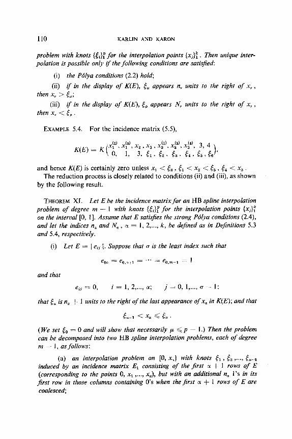
problem with knots {&}f for the interpolation points (xi}: . Then unique interpolation is possible only if the following conditions are satisfied:

(i) the Pdlya conditions (2.2) hold; (ii) if in the display of K(E), 6, appears n, units to the right of x, ,

then x, > E,; (iii) if in the display of K(E), 5, appears NV units to the right of x, ,

then x, < 5, .

EXAMPLE 5.4. For the incidence matrix (5.5),

(4’ 3, 4 K(E) = K ($2 xc, x2 , x3 9 x61), 2, x3 9 3, El > f3 3 (3 3 t4 I 5, > ‘5 ),

and hence K(E) is certainly zero unless x1 < 5, , 5, < x2 < & , f4 < x3 . The reduction process is closely related to conditions (ii) and (iii), as shown

by the following result.

THEOREM XI. Let E be the incidence matrix for an HB spline interpolation problem of degree m - 1 with knots (ti}T for the interpolation points {xi}: on the interval [0, I]. Assume that E satisfies the strong Pdlya conditions (2.4), and let the indices n, and N, , 01 = I, 2,..., k, be defined as in Dejinitions 5.3 and 5.4, respectively.

(i) Let E = I/ eij //. Suppose that (J is the least index such that

e o. = e,,,,, = ... = eo,m-l = 1

and that

eij = 0, i = 1, 2,..., ar; j = 0, I,..., u - I;

that 5, is n, + 1 units to the right of the last appearance of x, in K(E); and that

(We set to = 0 and will show that necessarily p ,< p - 1.) Then the problem can be decomposed into two HB spline interpolation problems, each qf degree m - 1, asfollows:

(a) an interpolation problem on [0, xdl] with knots fl, tz ,..., tU-1 induced by an incidence matrix El consisting of the first 01 f 1 rows of E (corresponding to the points 0, x1 ,..., xJ, but with an additional nar l’s in its first row in those columns containing O’s when the jirst cy + 1 rows of E are coalesced,


(b) a problem on [x, , l] with knots &, , [U+l ,..., 5, induced by an incidence matrix E, obtained from E by coalescing its first 01 + 1 rows. If 5, = xa 3 we replace e,,,-, = 1 by 0 in the reduced incidence matrix.

The original problem is decomposed in the sense that

W) = i WA) fWJ (5.6)

and we write E = E1 @ E, .

(ii) Suppose that r is the minimal index such that

ek+l.T = ek+1,7+1 = -*' = ektl,m--l = 1

and that

eij = 0, i = CX, c1 + I,..., k; j = 0, l,..., 7 - 1;

that 5, is N, - 1 units to the right of the first appearance of x, in K(E); and that

5‘” < & < Ll *

(We set e,+l = 1 and will show that v > 1.) Then the problem can be decomposed into two problems, each of degree m - 1, as follows:

(a) a problem on [0, x,] with knots tI, f2 ,..., &, induced by an incidence matrix E1 obtained from E by coalescing rows 01, 01 + l,..., k f 1 af E (and tf &, = x, , eoi.m-l = 1 in the coalesced matrix is to be replaced by 0);

(b) a problem on [x, , I] with knots Sy+l, tvf2 ,..., t, induced by an incidence matrix E, composed of rows 01, a f l,..., k + 1 of E (corresponding to the points x, , x,+~ ,..., I), with an additional m - N, l’s in the last row replacing the zeros which remain when these rows of E are coalesced.

The original problem is decomposed in the sense that (5.6) holds.

Remark 5.2. We give an example later to emphasize that this decomposition phenomenon is decisive in determining when HB spline interpolation problems are poised.

Our final result on HB spline interpolation states a sufficient condition for poisedness for one class of such problems.

THEOREM XII. Let E be an HB spline interpolation incidence matrix for a problem on [0, l] which prescribes either Hermite data or even blocks starting with the first derivative at points in (0, 1). Assume that E satisfies


the strong Pblya conditions, and that the interpolation points {xi}: and spline knots {&T satisfy:

(i) if& is n, + 1 units to the right of the last x, in K(E), then x, > &;; (ii) iftg is NV - 1 units to the right of thejirst x, in K(E), then xv < f, .

Then K(E) # 0; that is, the problem is poised.

The proof of this result is an easy consequence of Rolle’s theorem and the theorems elaborated by Karlin in [8]. Employing Sylvester’s determinant identity, it is easy to check that K(E) > 0 under the hypotheses of Theo- rem XII. Furthermore, it is a simple consequence of the interior rows of E containing no odd blocks that the signs in both (5.4) and (5.6), Proposition 5.1 and Theorem XI, respectively, are plus.

The hypotheses guarantee that the problem does not decompose at any interpolation point. The essential nature of this requirement is substantiated by the following example:

EXAMPLE 5.5. Consider the problem with incidence matrix

1 0 0 0 E=ollo

0 1 1 0 i10 0 0

Then n, = 1, n2 = 0, N1 = 4, N, = 3, and

(i) If x, < & or x, > & , then Theorem X shows that K(E) = 0, while according to Theorem X11, K(E) > 0 if x1 < & < & < x, .

(ii) If & < x2 < & , the problem decomposes at x2 into

1000 II II I/

1 1 1 1 ~~;~@I000 II

where the fist problem is for the points 0, x1, x2 with knot & , and the second, for x2 , 1 with knot c2 . It is clear that the second problem is poised, while by taking a derivative we find that the first is poised if and only if Xl -=c El <x2.

(iii) If [I < x1 < f2 , the problem decomposes at x1 into


where the first problem is for the points 0, x1 with knot & . Reasoning as above, we find that the problem is poised if and only if x1 < & < xz .

Summarizing, we find that K(E) > 0 if 0 < x, < & < x, < 1 or 0 -=c x1 -=c & -C xz < 1, and zero in all other cases. In particular, note that K(E) = 0 if .$ < x1 -=c x2 < & whereas, if we did not decompose, we would expect it to be nonzero from Theorem XII.

In view of the above example, sufficient conditions for unique spline interpolation involving even blocks starting at higher derivatives than the first are likely to be inherently complex.

6. OPEN QUESTIONS

1. The complete determination of exactly which HB polynomial incidence matrices satisfying the strong Polya conditions are order-poised appears to be intrinsically complicated. Necessary and sufficient conditions are known only for matrices each of whose interior rows contain at most one odd block: the problem is order-poised if and only if no odd block is supported (Proposition III and Theorem V). We have added to the class of matrices known to be non-poised with the sufficient conditions in Theorems V, VII, and VIII.

2. We have settled the question of unicity of HB spline interpolation only for Hermite data and even blocks beginning with the first derivative at interior points. It would be of interest to untangle complete criteria for unicity in more general circumstances. Apart from the independent interest of the problem, it is also of relevance for ascertaining unicity in best approximation of functions by monotone splines (in this connection, see Lorentz and Zeller [ 121).

3. We know of no studies on HB interpolation, either in the polynomial or spline case, with mixed conditions-i.e., interpolation conditions involving linear combinations of the values of the function and its derivatives at several points-except for periodic boundary conditions. Results for the latter case are elaborated in Karlin and Lee [lo].

4. It might be of interest to consider the possibility of polynomial interpolation by p(x) E TT,_~ of IZ - r interpolation conditions, and ask for conditions resulting in the smallest possible dimension of solutions, i.e., an r-dimensional variety of solutions.

5. There has been sparse accomplishment on deciding unicity of HB trigonometric interpolation (see Varma [21], and references therein, and also Karlin and Lee [lo]). More knowledge would be desirable.

114 KARLIN AND KARQN,

REFERENCES

1. J. H. AHLBERG, E. N. NIL~~N AND J. L. WALSH, “The Theory of Splines and Their Applications,” Academic Press, New York, 1967.

2. K. ATKINSON AND A. SHARMA, A partial characterization of poised Hermite-Birkhoff interpolation problems. SIAM J. Numer. Anal. 6 (1969), 230-235.

3. G. D. BIRKHOFF, General mean value and remainder theorems with applications to mechanical differentiation and integration. Trans. Amer. Math. Sot. 7 (1906), 107-136.

4. P. J. DA~J~, “Interpolation and Approximation,” Blaisdell, New York, 1963. 5. D. FERGUSON, The question of uniqueness for G. D. Birkhoff interpolation problems,

J. Approximation Theory 2 (1969), l-28. 6. T. N. E. GREVILLE, (Ed.), “Theory and Applications of Spline Functions,” Academic

Press, New York, 1969. 6a. J. W. JEROME, Linear self-adjoint multipoint boundary value problems and related

approximation schemes, Numer. Math. 15 (1970), 433449. 6b. J. W. JEROME AND L. L. SCHUMAKER, On Lg-splines, J. Approximation Theory 2 (1969).

29-49. 6c. J. W. JEROME AND L. L. SCHUMAKER, Local bases and computation of g-splines.

Univ. of Texas at Austin Center for Numerical Analysis Technical Report No. CNA3, 1970.

7. S. KARLIN, “Total Positivity,“. Vol. I, Stanford University Press, Stanford, CA, 1968.

8. S. KARLIN, Best quadrature formulas and interpolation by splines satisfying boundary conditions, in “Approximations with Special Emphasis on Spline Functions,” (I. J. Schoenberg, Ed.), pp. 447466, Academic Press, New York, 1969.

9. S. KARLIN AND J. KARON, Poised and non-poised HermiteBirkhoff interpolation problems, to appear in Indiana Univ. Math. J., 1972.

10. S. KARLIN AND J. L~ti, Periodic boundary value problems with cyclic totally positive Green’s functions with applications to periodic spline theory, to appear.

11. G. G. LORENTZ, Birkhoff interpolation and the problem of free matrices, to appear. 12. G. G. LDRENTZ AND K. L. ZELLER, Monotone approximation by algebraic polynomials,

Trans. Amer. Math. Sot. 149 (1970), 1-18. 13. G. G. LORENTZ AND K. L. ZELLER, Birkhoff interpolation, SIAM J. Numer. Anal.

8 (1971), 43-48. 14. 0. L. MANGA~ARIAN AND L. L. SCHUMAKER, Splines via optimal control, in “Approxi-

mations with Special Emphasis on Spline Functions,” (I. J. Schoenberg, Ed.), pp. pp. 119-156, Academic Press, New York, ,1969.

15. G. WLYA, Bemerkungen zur Interpolation und zur Naherungstheorie der Balken- biegung, Z. Angew. Math. Mech. 11 (1931), 445-449.

16. K. RIITER, Generalized spline interpolation and nonlinear programming, in “Approxi- mations with Special Emphasis on Spline Functions” (I. J. Schoenberg, Ed.), pp. 75-118, Academic Press, New York, 1969.

17. I. J. SCHOENBERG, On HermiteBirkhoff interpolation, J. Math. Anal. Appl. 16 (1966), 538-543.

18. I. J. SCHOENBERG, On the Ahlberg-Nilson extension of spline interpolation: G-splines and their optimal properties. J. Math. Anal. Appl. 21 (1968), 207-231.

19. I. J. SCHOENBERG, (Ed.), “Approximations with Special Emphasis on Spline Functions,” Academic Press, New York, 1969.

20. A. SHARMA AND J. PRASAD, On Abel-Hermite-Birkhoff interpolation, SZAM J. Numer. Anal. 5 (1968), 864-881.


21. A. K. VARMA, Simultaneous approximation of periodic continuous functions and their derivatives, Israel J. Math. 6 (1968), 66-73.

22. A. K. VAIWA, An analogue of a problem of J. BaHzs and P. Turan, III. Trans. Amer. Math. Sot. 146 (1969), 107-120.

23. A. SHAIWA, Some poised and nonpoised problems of interpolation, SIAM Rev. 14 (1972), 129-151.

24. C. A. MICCHELLI AND T. J. RIVLIN, Quadrature formulae and Hermite-Birkhoff interpolation, IBM Research Report RC 3396 (#15493), Yorktown Heights, N.Y., 1971.

Printed in Belgium

Documents

On Hermite-Birkhoff Interpolation*ON HERMITE-BIRKHOFF INTERPOLATION 95 Using a determinantal formulation of the problem, which is essential in this context, and arguments on the number