Embed Size (px)
Citation preview
12 Monthly Labor Review August 2003
Hispanic ConsumersHispanic Consumers
Geoffrey D. Paulin
Geoffrey D. Paulinis a senioreconomist in theDivision ofConsumer Expen-diture Surveys,Bureau of LaborStatistics. E-mail:[email protected].
As the composition of the Hispanic population changed,Hispanic consumers continued to increase their share of spendingat a substantial pace; a revisited study examines whether changesin expenditure patterns are due to changes in income or other similarfactors, or due to changes in underlying preferences
A changing market: expendituresby Hispanic consumers, revisited
The Hispanic population in the UnitedStates continues to grow. Accounting formore than 6 percent of the U.S. population
in 1980, the share nearly doubled by the year2000, with Hispanics accounting for just under12 percent of the population. 1 Growing at morethan 1 percent every 5 years since 1980, theHispanic population experienced its largestincrease during the 1995–2000 period, when itincreased nearly 1.5 percent. Similarly, Hispanicsaccount for an increasing portion of consumerspending—more than 6 percent in 1995 and morethan 7 percent in 2000.2
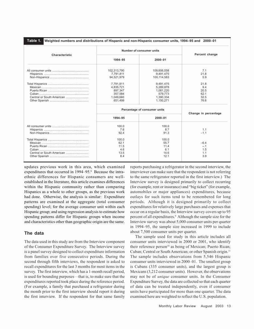
Many authors treat Hispanics as a homo-genous group, and have shown differences inexpenditure patterns from other groups, such asWhite and Black consumers.3 However, recentwork has shown that within the Hispaniccommunity, expenditure patterns differ sub-stantially by geographic origin. That is, familiesof Mexican origin spend differently from thoseof Puerto Rican, Cuban, or those of otherHispanic origin. This is true of expenditurepatterns in general,4 and for expenditures onspecific items, such as food.5 Due to thesedifferences, it is important to note that the sizeand composition of the U.S. Hispanic populationare changing. From 1994–95 to 2000–01, thenumber of Hispanic consumer units grew faster(21.8 percent) than the number of non-Hispanic
consumer units (5.9 percent).6 Among thoseHispanic consumer units, the growth rates rangedfrom 9.4 percent for Mexican families to 76.6percent for other Spanish families. The change incomposition can be seen when examining thedistribution of consumer units by ethnic origin.Although Mexican origin was still the largestsegment in 2000–01 (56 percent), it has fallen as ashare of all Hispanic consumer units since 1994–95 (62 percent). The Puerto Rican share was alittle more than 11 percent in both years, while allother groups saw increases in their shares ofHispanic families over the same time period.Cuban and Central or South American familiesincreased their shares between 1 percentage pointand 2 percentage points; those of other Spanishorigin increased their share by nearly 4 percentagepoints. (See table 1.) It is important to point outthat some of these changes are undoubtedly due tochanges in procedures used by the source fromwhich these data are obtained. However,independent sources also show differences ingrowth patterns within the Hispanic community.7
Given the diversity of expenditure patternsacross geographic origin, and the changingcomposition of the Hispanic market, it is importantto examine recent expenditure patterns for theHispanic population in the United States. Inaddition to examining the most recent dataavailable, that is, data from 2000–01, this article
Monthly Labor Review August 2003 13
Table 1. Weighted numbers and distributions of Hispanic and non-Hispanic consumer units, 1994–95 and 2000–01
Number of consumer units
1994–95 2000–01
All consumer units ............................................. 102,313,790 109,606,058 7.1Hispanics ....................................................... 7,791,811 9,491,475 21.8Non-Hispanics ................................................ 94,521,979 100,114,583 5.9
...........................................................................Total Hispanics .................................................. 7,791,811 9,491,475 21.8
Mexican .......................................................... 4,835,721 5,289,878 9.4Puerto Rican .................................................. 897,347 1,081,220 20.5Cuban ............................................................. 357,584 579,773 62.1Central or South American ............................ 1,049,660 1,390,334 32.5Other Spanish ................................................ 651,499 1,150,271 76.6
Percentage of consumer units
1994–95 2000–01
All consumer units ............................................. 100.0 100.0Hispanics ....................................................... 7.6 8.7 1.1Non-Hispanics ................................................ 92.4 91.3 –1.1
Total Hispanics .................................................. 100.0 100.0Mexican .......................................................... 62.1 55.7 –6.4Puerto Rican .................................................. 11.5 11.4 –.1Cuban ............................................................. 4.6 6.1 1.5Central or South American ............................ 13.5 14.6 1.1Other Spanish ................................................ 8.4 12.1 3.9
Change in percentage
updates previous work in this area, which examinedexpenditures that occurred in 1994–95.8 Because the intra-ethnic differences for Hispanic consumers are well-established in the literature, this article examines differenceswithin the Hispanic community rather than comparingHispanics as a whole to other groups, as the previous workhad done. Otherwise, the analysis is similar: Expenditurepatterns are examined at the aggregate (total consumerspending) level; for the average consumer unit within eachHispanic group; and using regression analysis to estimate howspending patterns differ for Hispanic groups when incomeand characteristics other than geographic origin are the same.
The data
The data used in this study are from the Interview componentof the Consumer Expenditure Survey. The Interview surveyis a panel survey designed to collect expenditure informationfrom families over five consecutive periods. During thesecond through fifth interviews, the respondent is asked torecall expenditures for the last 3 months for most items in thesurvey. The first interview, which has a 1-month recall period,is used for bounding purposes—that is, to make sure that theexpenditures reported took place during the reference period.(For example, a family that purchased a refrigerator duringthe month prior to the first interview should report it duringthe first interview. If the respondent for that same family
reports purchasing a refrigerator in the second interview, theinterviewer can make sure that the respondent is not referringto the same refrigerator reported in the first interview.) TheInterview survey is designed primarily to collect recurring(for example, rent or insurance) and “big ticket” (for example,automobiles or major appliances) expenditures, becauseoutlays for such items tend to be remembered for longperiods. Although it is designed primarily to collectexpenditures for relatively large purchases and expenses thatoccur on a regular basis, the Interview survey covers up to 95percent of all expenditures.9 Although the sample size for theInterview survey was about 5,000 consumer units per quarterin 1994–95, the sample size increased in 1999 to includeabout 7,500 consumer units per quarter.
The sample used for study in this article includes allconsumer units interviewed in 2000 or 2001, who identifytheir reference person10 as being of Mexican; Puerto Rican;Cuban; Central or South American; or other Spanish origin.11
The sample includes observations from 5,546 Hispanicconsumer units interviewed in 2000–01. The smallest groupis Cubans (335 consumer units), and the largest group isMexicans (3,212 consumer units). However, the observationsmay not be of unique consumer units. In the ConsumerExpenditure Survey, the data are collected so that each quarterof data can be treated independently, even if consumerunits have participated for more than one quarter. The dataexamined here are weighted to reflect the U.S. population.
Percent changeCharacteristic
14 Monthly Labor Review August 2003
Hispanic Consumers
Demographic characteristics
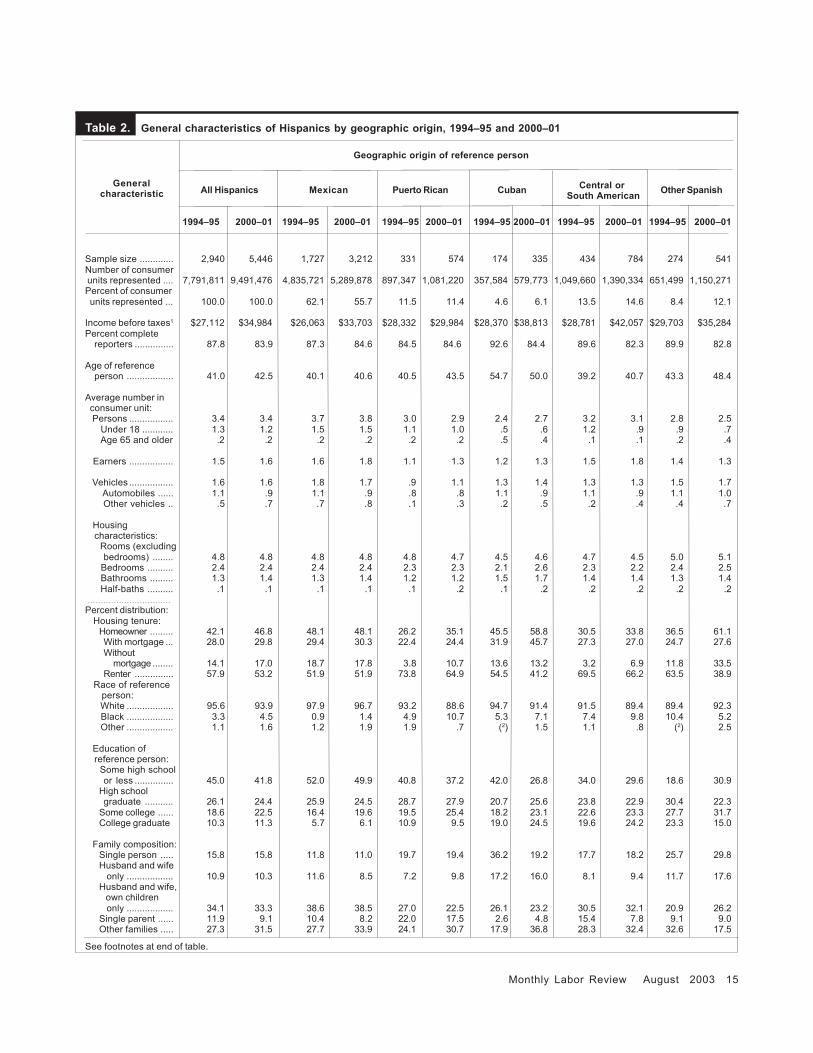
Among the several demographic characteristics for each ofthe Hispanic groups under study, income before taxes and age ofreference person appear to have changed substantially over the1994–95 to 2000–01 period. (See table 2.) On average, incomebefore taxes appears to have experienced increases over timefor complete income reporters.12 The smallest increase is forPuerto Ricans (5.8 percent); the largest is for Central or SouthAmericans (46.1 percent). Except for Puerto Ricans and otherSpanish families, these increases all are statisticallysignificant. However, these changes are only correct fornominal income. The Consumer Price Index (CPI) rose from150.3 in the 1994–95 period to 174.7 in 2000–01; an increaseof 16.2 percent. After adjusting for inflation, the outcomesare very different. Puerto Ricans had lower earnings in real(that is, inflation-adjusted) dollars (−8.9 percent). Incomefor all other groups increased, but at varying rates. OtherSpanish real income rose 2.2 percent, while income forCentral or South Americans rose 25.8 percent in real terms.Furthermore, none of these changes (increases or declines) isstatistically significant for any individual group, oncevariance is taken into account. Similarly, over the sameperiod, age of reference person appears to have changed forseveral groups. Relatively large changes in average ageappear for Puerto Rican, Cuban, and other Spanish families.However, when the variance in each year is taken intoaccount, the changes in age are not found to be statisticallysignificant.
Several demographics for which percent reporting isshown have also changed, and in ways that one wouldprobably associate with improved economic status. Forexample, the percentage of homeowners increased for allHispanics from 42 percent to nearly 47 percent over the studyperiod. In particular, large changes are seen for Puerto Ricans(26 to 35 percent); Cubans (46 to 59 percent); and otherSpanish families (37 to 61 percent). Educational attainmenthas also increased for most groups, with declines in highschool or less education, and increases in percent reportingat least some college. The exception is other Spanish families,for whom the percent reporting some high school or less rosesharply, from 19 percent to 31 percent. In contrast, the percentreporting high school graduation dropped from 30 percent to22 percent. Similarly, the percentage of college graduatesdropped from 23 percent to 15 percent. Other than the groupof some high school or less, only the group with some collegeincreased, from 28 percent to 32 percent among thosereporting for other Spanish families. Several groups alsoreported higher percentages of reference persons for theirconsumer units who were working for pay. For example,Puerto Ricans reported 60 percent working (58 percent for awage or salary; 2 percent self-employed) in 1994–95,compared with 68 percent in 2000–01. Although the percent
retired rose, from 7 percent to 10 percent, for this group, theproportion not working for reasons other than retirement fellfrom 34 percent to 24 percent. Similarly, Central or SouthAmerican households reported 78 percent of referencepersons working in 1994–95, and 19 percent not working forreason other than retirement. However, in 2000–01, theworking proportion rose to 84 percent, and the other-reasons-not-working proportion fell to 11 percent. In most other cases,the proportions were similar in each period, with theexception of other Spanish households. For this group, thepercent reporting that the reference person works droppedfrom 70 percent to 66 percent. Wage and salary reportersdropped from 67 to 60 percent, while reports of self-employment rose from 3 percent to 6 percent. The largestchange, though, was in retirement: 9 percent of these otherSpanish households reported a retired reference person in1994–95, compared with 20 percent in 2000–01. At the sametime, the percent reporting reference persons not working forreasons other than retirement dropped from more than 1 in 5to about 1 in 7. Whether the changes in occupational statusindicate higher economic status is an open question. It maybe that the “others not working for pay” rate was higher in1994–95 than 2000–01 because more families in 1994–95could afford to have the reference person stay at home thanthose could in 2000–01. (One of the reasons for “others notworking pay,” for example, is staying home to take care ofchildren or family members.) If the changes described in thecomposition of the Hispanic community are due to increasesin immigration by different groups, this also could play a role,as it is reasonable to assume that the desire to work is a majorfactor in the decision to immigrate.13
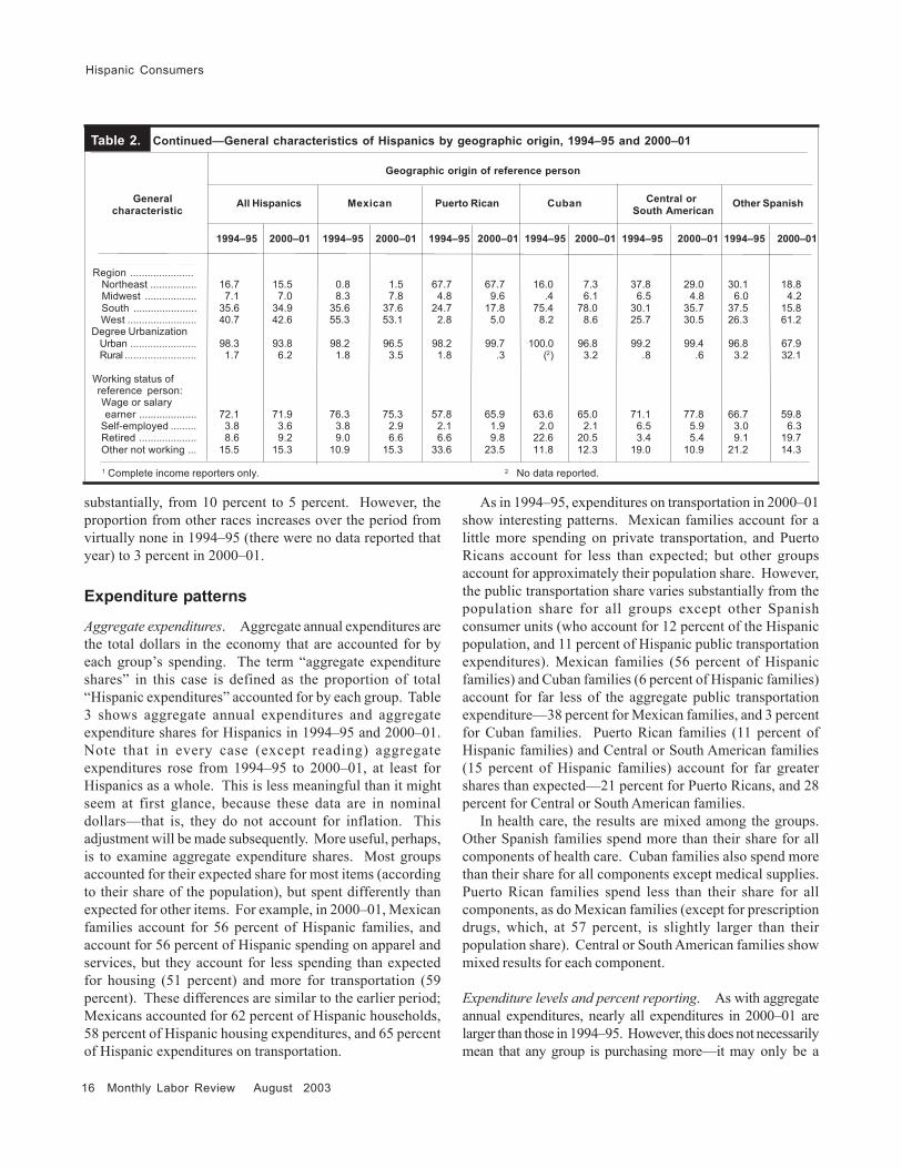
Other characteristics were stable over the period. Forexample, family composition did not change much for mostHispanic families, except for Cubans, who are less likely tobe single and more likely to be “other families” in 2000–01than in 1994–95. Similarly, other Spanish familiesexperienced an increase in married-couple families (with andwithout children) and a decrease in other families. Degree ofurbanization did not change substantially, except for otherSpanish families; for this group in 1994–95, there were about30 urban families for every rural family; but in 2000–01, therewere only 2 urban families for every rural family.
Changes by region are also interesting. Except for Mexicanand Puerto Rican families, all groups show smallerproportions in the Northeast in 2000–01 than in 1994–95.Which region experiences growth at the expense of theNortheast’s decline is different across Hispanic groups.
All groups but one show increases in the proportion ofnon-White families. The exception is other Spanish, forwhich the proportion of White families rises from 89 percentto 92 percent, and the proportion of Black families declines
Monthly Labor Review August 2003 15
Table 2. General characteristics of Hispanics by geographic origin, 1994–95 and 2000–01
Geographic origin of reference person
All Hispanics Mexican Puerto Rican Cuban Other Spanish
1994–95 2000–01 1994–95 2000–01 1994–95 2000–01 1994–95 2000–01 1994–95 2000–01 1994–95 2000–01
Sample size ............. 2,940 5,446 1,727 3,212 331 574 174 335 434 784 274 541Number of consumer units represented .... 7,791,811 9,491,476 4,835,721 5,289,878 897,347 1,081,220 357,584 579,773 1,049,660 1,390,334 651,499 1,150,271Percent of consumerunits represented ... 100.0 100.0 62.1 55.7 11.5 11.4 4.6 6.1 13.5 14.6 8.4 12.1
Income before taxes1 $27,112 $34,984 $26,063 $33,703 $28,332 $29,984 $28,370 $38,813 $28,781 $42,057 $29,703 $35,284Percent complete
reporters ............... 87.8 83.9 87.3 84.6 84.5 84.6 92.6 84.4 89.6 82.3 89.9 82.8.................................Age of reference
person .................. 41.0 42.5 40.1 40.6 40.5 43.5 54.7 50.0 39.2 40.7 43.3 48.4................................ Average number inconsumer unit:
Persons ................. 3.4 3.4 3.7 3.8 3.0 2.9 2.4 2.7 3.2 3.1 2.8 2.5 Under 18 ............ 1.3 1.2 1.5 1.5 1.1 1.0 .5 .6 1.2 .9 .9 .7 Age 65 and older .2 .2 .2 .2 .2 .2 .5 .4 .1 .1 .2 .4................................ Earners ................. 1.5 1.6 1.6 1.8 1.1 1.3 1.2 1.3 1.5 1.8 1.4 1.3................................ Vehicles ................. 1.6 1.6 1.8 1.7 .9 1.1 1.3 1.4 1.3 1.3 1.5 1.7 Automobiles ...... 1.1 .9 1.1 .9 .8 .8 1.1 .9 1.1 .9 1.1 1.0 Other vehicles .. .5 .7 .7 .8 .1 .3 .2 .5 .2 .4 .4 .7................................ Housing
characteristics: Rooms (excluding
bedrooms) ........ 4.8 4.8 4.8 4.8 4.8 4.7 4.5 4.6 4.7 4.5 5.0 5.1 Bedrooms .......... 2.4 2.4 2.4 2.4 2.3 2.3 2.1 2.6 2.3 2.2 2.4 2.5 Bathrooms ......... 1.3 1.4 1.3 1.4 1.2 1.2 1.5 1.7 1.4 1.4 1.3 1.4 Half-baths .......... .1 .1 .1 .1 .1 .2 .1 .2 .2 .2 .2 .2................................ Percent distribution: Housing tenure:
Homeowner ......... 42.1 46.8 48.1 48.1 26.2 35.1 45.5 58.8 30.5 33.8 36.5 61.1With mortgage ... 28.0 29.8 29.4 30.3 22.4 24.4 31.9 45.7 27.3 27.0 24.7 27.6Without
mortgage ........ 14.1 17.0 18.7 17.8 3.8 10.7 13.6 13.2 3.2 6.9 11.8 33.5Renter ............... 57.9 53.2 51.9 51.9 73.8 64.9 54.5 41.2 69.5 66.2 63.5 38.9
Race of reference person: White .................. 95.6 93.9 97.9 96.7 93.2 88.6 94.7 91.4 91.5 89.4 89.4 92.3 Black .................. 3.3 4.5 0.9 1.4 4.9 10.7 5.3 7.1 7.4 9.8 10.4 5.2 Other .................. 1.1 1.6 1.2 1.9 1.9 .7 (2) 1.5 1.1 .8 (2) 2.5................................ Education of
reference person: Some high school
or less ............... 45.0 41.8 52.0 49.9 40.8 37.2 42.0 26.8 34.0 29.6 18.6 30.9High schoolgraduate ........... 26.1 24.4 25.9 24.5 28.7 27.9 20.7 25.6 23.8 22.9 30.4 22.3
Some college ...... 18.6 22.5 16.4 19.6 19.5 25.4 18.2 23.1 22.6 23.3 27.7 31.7College graduate 10.3 11.3 5.7 6.1 10.9 9.5 19.0 24.5 19.6 24.2 23.3 15.0
................................ Family composition:
Single person ..... 15.8 15.8 11.8 11.0 19.7 19.4 36.2 19.2 17.7 18.2 25.7 29.8Husband and wife only .................. 10.9 10.3 11.6 8.5 7.2 9.8 17.2 16.0 8.1 9.4 11.7 17.6
Husband and wife, own children only .................. 34.1 33.3 38.6 38.5 27.0 22.5 26.1 23.2 30.5 32.1 20.9 26.2
Single parent ...... 11.9 9.1 10.4 8.2 22.0 17.5 2.6 4.8 15.4 7.8 9.1 9.0Other families ..... 27.3 31.5 27.7 33.9 24.1 30.7 17.9 36.8 28.3 32.4 32.6 17.5
See footnotes at end of table.
Generalcharacteristic
Central or South American
16 Monthly Labor Review August 2003
Hispanic Consumers
............................. ...... Region ...................... Northeast ................ 16.7 15.5 0.8 1.5 67.7 67.7 16.0 7.3 37.8 29.0 30.1 18.8 Midwest .................. 7.1 7.0 8.3 7.8 4.8 9.6 .4 6.1 6.5 4.8 6.0 4.2 South ...................... 35.6 34.9 35.6 37.6 24.7 17.8 75.4 78.0 30.1 35.7 37.5 15.8 West ........................ 40.7 42.6 55.3 53.1 2.8 5.0 8.2 8.6 25.7 30.5 26.3 61.2 Degree Urbanization: .
Urban ....................... 98.3 93.8 98.2 96.5 98.2 99.7 100.0 96.8 99.2 99.4 96.8 67.9Rural ......................... 1.7 6.2 1.8 3.5 1.8 .3 (2) 3.2 .8 .6 3.2 32.1
..................................... Working status of
reference person: .... Wage or salary
earner .................... 72.1 71.9 76.3 75.3 57.8 65.9 63.6 65.0 71.1 77.8 66.7 59.8 Self-employed ......... 3.8 3.6 3.8 2.9 2.1 1.9 2.0 2.1 6.5 5.9 3.0 6.3 Retired .................... 8.6 9.2 9.0 6.6 6.6 9.8 22.6 20.5 3.4 5.4 9.1 19.7 Other not working ... 15.5 15.3 10.9 15.3 33.6 23.5 11.8 12.3 19.0 10.9 21.2 14.3.................................
1 Complete income reporters only. 2 No data reported.
Table 2. Continued—General characteristics of Hispanics by geographic origin, 1994–95 and 2000–01
Geographic origin of reference person
All Hispanics Mexican Puerto Rican Cuban Other Spanish
1994–95 2000–01 1994–95 2000–01 1994–95 2000–01 1994–95 2000–01 1994–95 2000–01 1994–95 2000–01
Generalcharacteristic
substantially, from 10 percent to 5 percent. However, theproportion from other races increases over the period fromvirtually none in 1994–95 (there were no data reported thatyear) to 3 percent in 2000–01.
Expenditure patterns
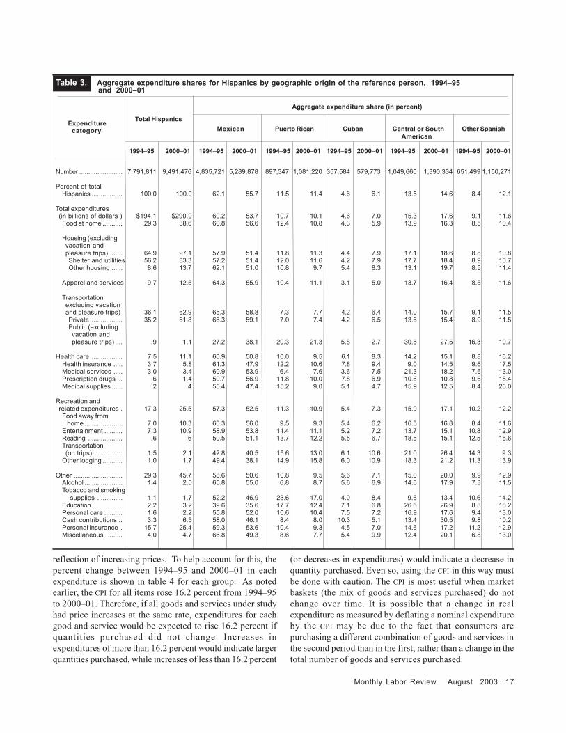
Aggregate expenditures. Aggregate annual expenditures arethe total dollars in the economy that are accounted for byeach group’s spending. The term “aggregate expenditureshares” in this case is defined as the proportion of total“Hispanic expenditures” accounted for by each group. Table3 shows aggregate annual expenditures and aggregateexpenditure shares for Hispanics in 1994–95 and 2000–01.Note that in every case (except reading) aggregateexpenditures rose from 1994–95 to 2000–01, at least forHispanics as a whole. This is less meaningful than it mightseem at first glance, because these data are in nominaldollars—that is, they do not account for inflation. Thisadjustment will be made subsequently. More useful, perhaps,is to examine aggregate expenditure shares. Most groupsaccounted for their expected share for most items (accordingto their share of the population), but spent differently thanexpected for other items. For example, in 2000–01, Mexicanfamilies account for 56 percent of Hispanic families, andaccount for 56 percent of Hispanic spending on apparel andservices, but they account for less spending than expectedfor housing (51 percent) and more for transportation (59percent). These differences are similar to the earlier period;Mexicans accounted for 62 percent of Hispanic households,58 percent of Hispanic housing expenditures, and 65 percentof Hispanic expenditures on transportation.
As in 1994–95, expenditures on transportation in 2000–01show interesting patterns. Mexican families account for alittle more spending on private transportation, and PuertoRicans account for less than expected; but other groupsaccount for approximately their population share. However,the public transportation share varies substantially from thepopulation share for all groups except other Spanishconsumer units (who account for 12 percent of the Hispanicpopulation, and 11 percent of Hispanic public transportationexpenditures). Mexican families (56 percent of Hispanicfamilies) and Cuban families (6 percent of Hispanic families)account for far less of the aggregate public transportationexpenditure—38 percent for Mexican families, and 3 percentfor Cuban families. Puerto Rican families (11 percent ofHispanic families) and Central or South American families(15 percent of Hispanic families) account for far greatershares than expected—21 percent for Puerto Ricans, and 28percent for Central or South American families.
In health care, the results are mixed among the groups.Other Spanish families spend more than their share for allcomponents of health care. Cuban families also spend morethan their share for all components except medical supplies.Puerto Rican families spend less than their share for allcomponents, as do Mexican families (except for prescriptiondrugs, which, at 57 percent, is slightly larger than theirpopulation share). Central or South American families showmixed results for each component.
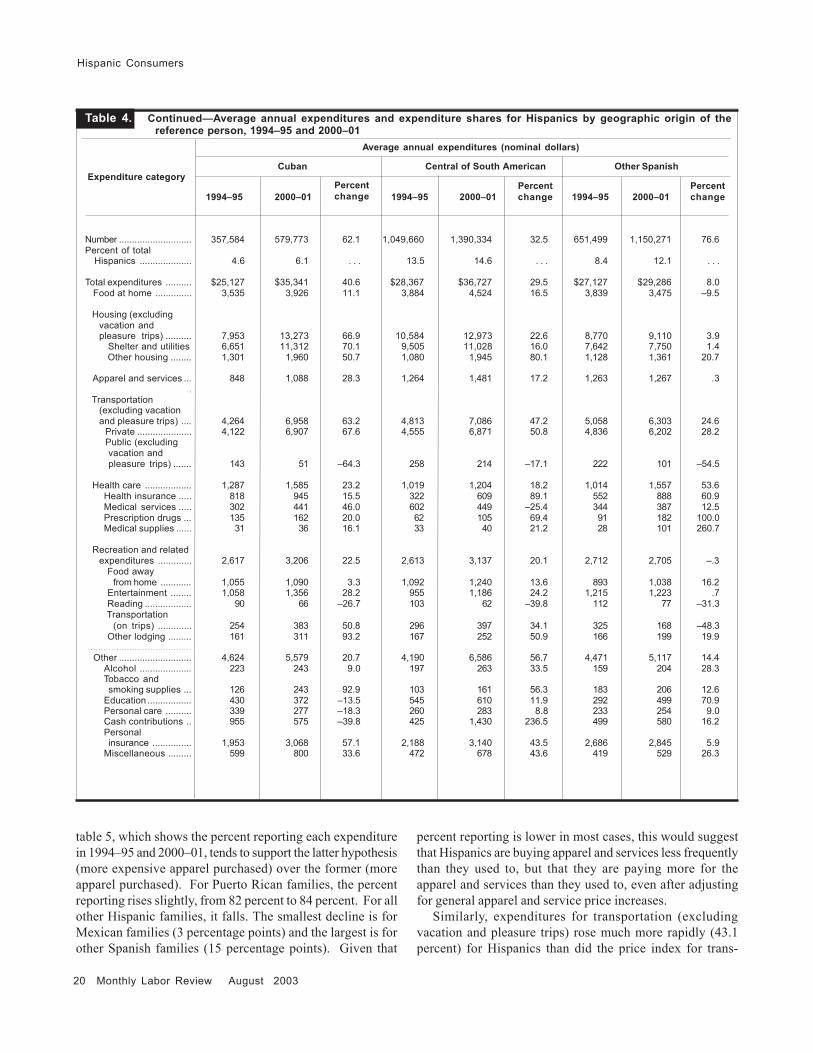
Expenditure levels and percent reporting. As with aggregateannual expenditures, nearly all expenditures in 2000–01 arelarger than those in 1994–95. However, this does not necessarilymean that any group is purchasing more—it may only be a
Central or South American
Monthly Labor Review August 2003 17
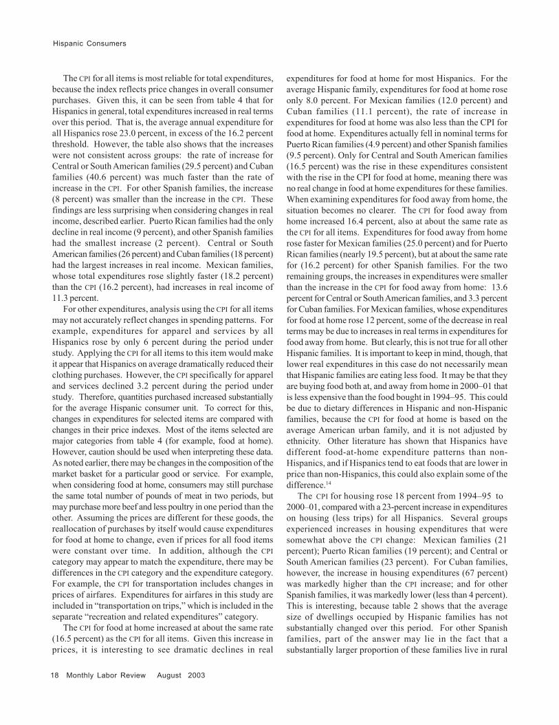
reflection of increasing prices. To help account for this, thepercent change between 1994–95 and 2000–01 in eachexpenditure is shown in table 4 for each group. As notedearlier, the CPI for all items rose 16.2 percent from 1994–95to 2000–01. Therefore, if all goods and services under studyhad price increases at the same rate, expenditures for eachgood and service would be expected to rise 16.2 percent ifquantities purchased did not change. Increases inexpenditures of more than 16.2 percent would indicate largerquantities purchased, while increases of less than 16.2 percent
Table 3. Aggregate expenditure shares for Hispanics by geographic origin of the reference person, 1994–95 and 2000–01
Aggregate expenditure share (in percent)
Mexican Puerto Rican Cuban Central or South Other SpanishAmerican
1994–95 2000–01 1994–95 2000–01 1994–95 2000–01 1994–95 2000–01 1994–95 2000–01 1994–95 2000–01
Number ........................ 7,791,811 9,491,476 4,835,721 5,289,878 897,347 1,081,220 357,584 579,773 1,049,660 1,390,334 651,499 1,150,271
Percent of totalHispanics ................. 100.0 100.0 62.1 55.7 11.5 11.4 4.6 6.1 13.5 14.6 8.4 12.1
................................... Total expenditures(in billions of dollars ) $194.1 $290.9 60.2 53.7 10.7 10.1 4.6 7.0 15.3 17.6 9.1 11.6Food at home ........... 29.3 38.6 60.8 56.6 12.4 10.8 4.3 5.9 13.9 16.3 8.5 10.4
Housing (excludingvacation andpleasure trips) ....... 64.9 97.1 57.9 51.4 11.8 11.3 4.4 7.9 17.1 18.6 8.8 10.8Shelter and utilities 56.2 83.3 57.2 51.4 12.0 11.6 4.2 7.9 17.7 18.4 8.9 10.7Other housing ...... 8.6 13.7 62.1 51.0 10.8 9.7 5.4 8.3 13.1 19.7 8.5 11.4
Apparel and services 9.7 12.5 64.3 55.9 10.4 11.1 3.1 5.0 13.7 16.4 8.5 11.6
Transportationexcluding vacationand pleasure trips) 36.1 62.9 65.3 58.8 7.3 7.7 4.2 6.4 14.0 15.7 9.1 11.5Private .................. 35.2 61.8 66.3 59.1 7.0 7.4 4.2 6.5 13.6 15.4 8.9 11.5Public (excludingvacation andpleasure trips) .... .9 1.1 27.2 38.1 20.3 21.3 5.8 2.7 30.5 27.5 16.3 10.7
Health care .................. 7.5 11.1 60.9 50.8 10.0 9.5 6.1 8.3 14.2 15.1 8.8 16.2Health insurance ..... 3.7 5.8 61.3 47.9 12.2 10.6 7.8 9.4 9.0 14.5 9.6 17.5Medical services ..... 3.0 3.4 60.9 53.9 6.4 7.6 3.6 7.5 21.3 18.2 7.6 13.0Prescription drugs ... .6 1.4 59.7 56.9 11.8 10.0 7.8 6.9 10.6 10.8 9.6 15.4Medical supplies ...... .2 .4 55.4 47.4 15.2 9.0 5.1 4.7 15.9 12.5 8.4 26.0
Recreation andrelated expenditures . 17.3 25.5 57.3 52.5 11.3 10.9 5.4 7.3 15.9 17.1 10.2 12.2Food away from home ..................... 7.0 10.3 60.3 56.0 9.5 9.3 5.4 6.2 16.5 16.8 8.4 11.6
Entertainment .......... 7.3 10.9 58.9 53.8 11.4 11.1 5.2 7.2 13.7 15.1 10.8 12.9Reading ................... .6 .6 50.5 51.1 13.7 12.2 5.5 6.7 18.5 15.1 12.5 15.6Transportation(on trips) ................ 1.5 2.1 42.8 40.5 15.6 13.0 6.1 10.6 21.0 26.4 14.3 9.3
Other lodging ........... 1.0 1.7 49.4 38.1 14.9 15.8 6.0 10.9 18.3 21.2 11.3 13.9
Other ........................... 29.3 45.7 58.6 50.6 10.8 9.5 5.6 7.1 15.0 20.0 9.9 12.9Alcohol ..................... 1.4 2.0 65.8 55.0 6.8 8.7 5.6 6.9 14.6 17.9 7.3 11.5Tobacco and smoking
supplies .............. 1.1 1.7 52.2 46.9 23.6 17.0 4.0 8.4 9.6 13.4 10.6 14.2Education ................ 2.2 3.2 39.6 35.6 17.7 12.4 7.1 6.8 26.6 26.9 8.8 18.2Personal care .......... 1.6 2.2 55.8 52.0 10.6 10.4 7.5 7.2 16.9 17.6 9.4 13.0Cash contributions .. 3.3 6.5 58.0 46.1 8.4 8.0 10.3 5.1 13.4 30.5 9.8 10.2Personal insurance . 15.7 25.4 59.3 53.6 10.4 9.3 4.5 7.0 14.6 17.2 11.2 12.9Miscellaneous ......... 4.0 4.7 66.8 49.3 8.6 7.7 5.4 9.9 12.4 20.1 6.8 13.0
Expenditurecategory
(or decreases in expenditures) would indicate a decrease inquantity purchased. Even so, using the CPI in this way mustbe done with caution. The CPI is most useful when marketbaskets (the mix of goods and services purchased) do notchange over time. It is possible that a change in realexpenditure as measured by deflating a nominal expenditureby the CPI may be due to the fact that consumers arepurchasing a different combination of goods and services inthe second period than in the first, rather than a change in thetotal number of goods and services purchased.
Total Hispanics
18 Monthly Labor Review August 2003
Hispanic Consumers
The CPI for all items is most reliable for total expenditures,because the index reflects price changes in overall consumerpurchases. Given this, it can be seen from table 4 that forHispanics in general, total expenditures increased in real termsover this period. That is, the average annual expenditure forall Hispanics rose 23.0 percent, in excess of the 16.2 percentthreshold. However, the table also shows that the increaseswere not consistent across groups: the rate of increase forCentral or South American families (29.5 percent) and Cubanfamilies (40.6 percent) was much faster than the rate ofincrease in the CPI. For other Spanish families, the increase(8 percent) was smaller than the increase in the CPI. Thesefindings are less surprising when considering changes in realincome, described earlier. Puerto Rican families had the onlydecline in real income (9 percent), and other Spanish familieshad the smallest increase (2 percent). Central or SouthAmerican families (26 percent) and Cuban families (18 percent)had the largest increases in real income. Mexican families,whose total expenditures rose slightly faster (18.2 percent)than the CPI (16.2 percent), had increases in real income of11.3 percent.
For other expenditures, analysis using the CPI for all itemsmay not accurately reflect changes in spending patterns. Forexample, expenditures for apparel and services by allHispanics rose by only 6 percent during the period understudy. Applying the CPI for all items to this item would makeit appear that Hispanics on average dramatically reduced theirclothing purchases. However, the CPI specifically for appareland services declined 3.2 percent during the period understudy. Therefore, quantities purchased increased substantiallyfor the average Hispanic consumer unit. To correct for this,changes in expenditures for selected items are compared withchanges in their price indexes. Most of the items selected aremajor categories from table 4 (for example, food at home).However, caution should be used when interpreting these data.As noted earlier, there may be changes in the composition of themarket basket for a particular good or service. For example,when considering food at home, consumers may still purchasethe same total number of pounds of meat in two periods, butmay purchase more beef and less poultry in one period than theother. Assuming the prices are different for these goods, thereallocation of purchases by itself would cause expendituresfor food at home to change, even if prices for all food itemswere constant over time. In addition, although the CPIcategory may appear to match the expenditure, there may bedifferences in the CPI category and the expenditure category.For example, the CPI for transportation includes changes inprices of airfares. Expenditures for airfares in this study areincluded in “transportation on trips,” which is included in theseparate “recreation and related expenditures” category.
The CPI for food at home increased at about the same rate(16.5 percent) as the CPI for all items. Given this increase inprices, it is interesting to see dramatic declines in real
expenditures for food at home for most Hispanics. For theaverage Hispanic family, expenditures for food at home roseonly 8.0 percent. For Mexican families (12.0 percent) andCuban families (11.1 percent), the rate of increase inexpenditures for food at home was also less than the CPI forfood at home. Expenditures actually fell in nominal terms forPuerto Rican families (4.9 percent) and other Spanish families(9.5 percent). Only for Central and South American families(16.5 percent) was the rise in these expenditures consistentwith the rise in the CPI for food at home, meaning there wasno real change in food at home expenditures for these families.When examining expenditures for food away from home, thesituation becomes no clearer. The CPI for food away fromhome increased 16.4 percent, also at about the same rate asthe CPI for all items. Expenditures for food away from homerose faster for Mexican families (25.0 percent) and for PuertoRican families (nearly 19.5 percent), but at about the same ratefor (16.2 percent) for other Spanish families. For the tworemaining groups, the increases in expenditures were smallerthan the increase in the CPI for food away from home: 13.6percent for Central or South American families, and 3.3 percentfor Cuban families. For Mexican families, whose expendituresfor food at home rose 12 percent, some of the decrease in realterms may be due to increases in real terms in expenditures forfood away from home. But clearly, this is not true for all otherHispanic families. It is important to keep in mind, though, thatlower real expenditures in this case do not necessarily meanthat Hispanic families are eating less food. It may be that theyare buying food both at, and away from home in 2000–01 thatis less expensive than the food bought in 1994–95. This couldbe due to dietary differences in Hispanic and non-Hispanicfamilies, because the CPI for food at home is based on theaverage American urban family, and it is not adjusted byethnicity. Other literature has shown that Hispanics havedifferent food-at-home expenditure patterns than non-Hispanics, and if Hispanics tend to eat foods that are lower inprice than non-Hispanics, this could also explain some of thedifference.14
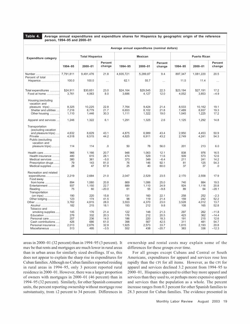
The CPI for housing rose 18 percent from 1994–95 to2000–01, compared with a 23-percent increase in expenditureson housing (less trips) for all Hispanics. Several groupsexperienced increases in housing expenditures that weresomewhat above the CPI change: Mexican families (21percent); Puerto Rican families (19 percent); and Central orSouth American families (23 percent). For Cuban families,however, the increase in housing expenditures (67 percent)was markedly higher than the CPI increase; and for otherSpanish families, it was markedly lower (less than 4 percent).This is interesting, because table 2 shows that the averagesize of dwellings occupied by Hispanic families has notsubstantially changed over this period. For other Spanishfamilies, part of the answer may lie in the fact that asubstantially larger proportion of these families live in rural
Monthly Labor Review August 2003 19
areas in 2000–01 (32 percent) than in 1994–95 (3 percent). Itmay be that rents and mortgages are much lower in rural areasthan in urban areas for similarly sized dwellings. If so, thisdoes not appear to explain the sharp rise in expenditures forCuban families. Although no Cuban families reported residingin rural areas in 1994–95, only 3 percent reported ruralresidence in 2000–01. However, there was a larger proportionof owners with mortgages in 2000–01 (46 percent) than in1994–95 (32 percent). Similarly, for other Spanish consumerunits, the percent reporting ownership without mortgage rosesubstantially, from 12 percent to 34 percent. Differences in
ownership and rental costs may explain some of thedifferences for these groups over time.
For all groups except Cubans and Central or SouthAmericans, expenditures for apparel and services rose lessrapidly than the CPI for all items. However, as the CPI forapparel and services declined 3.2 percent from 1994–95 to2000–01, Hispanics appeared to either buy more apparel andservices than they used to, or perhaps more expensive appareland services than the population as a whole. The percentincrease ranges from 0.3 percent for other Spanish families to28.3 percent for Cuban families. The evidence presented in
Table 4. Average annual expenditures and expenditure shares for Hispanics by geographic origin of the reference person, 1994–95 and 2000–01
Number .............................. 7,791,811 9,491,476 21.8 4,835,721 5,289,87 9.4 897,347 1,081,220 20.5Percent of total
Hispanics ....................... 100.0 100.0 ... 62.1 55.7 ... 11.5 11.4 ...
......................................... Total expenditures ............ $24,911 $30,651 23.0 $24,164 $29,545 22.3 $23,194 $27,191 17.2 Food at home ................ 3,761 4,063 8.0 3,686 4,127 12.0 4,052 3,853 –4.9 .........................................
Housing (excludingvacation andpleasure trips) ............ 8,325 10,225 22.8 7,764 9,424 21.4 8,533 10,162 19.1Shelter and utilities .... 7,216 8,779 21.7 6,653 8,102 21.8 7,489 8,937 19.3Other housing ............ 1,110 1,446 30.3 1,111 1,322 19.0 1,045 1,225 17.2
......................................... Apparel and services .... 1,246 1,322 6.1 1,291 1,325 2.6 1,125 1,292 14.8 ......................................... Transportation
(excluding vacationand pleasure trips) ..... 4,632 6,629 43.1 4,875 6,989 43.4 2,950 4,453 50.9
Private ......................... 4,518 6,515 44.2 4,825 6,911 43.2 2,749 4,241 54.3Public (excluding
vacation andpleasure trips) .......... 114 114 .0 50 78 56.0 201 213 6.0
Health care .................... 966 1,166 20.7 948 1,063 12.1 838 976 16.5Health insurance ......... 480 615 28.1 474 529 11.6 509 573 12.6Medical services ......... 380 361 –5.0 373 349 –6.4 211 241 14.2Prescription drugs ....... 79 143 81.0 76 146 92.1 81 125 54.3Medical supplies .......... 28 47 67.9 25 40 60.0 37 37 .0
........................................ Recreation and related
expenditures ................. 2,219 2,684 21.0 2,047 2,529 23.5 2,170 2,558 17.9Food awayfrom home .................. 894 1,080 20.8 869 1,086 25.0 740 884 19.5
Entertainment .............. 937 1,150 22.7 889 1,110 24.9 924 1,116 20.8Reading ........................ 75 60 –20.0 61 55 –9.8 89 64 –28.1Transportation (on trips) ................... 190 220 15.8 131 160 22.1 258 252 –2.3
Other lodging ............... 123 174 41.5 98 119 21.4 159 242 52.2 Other .............................. 3,762 4,815 28.0 3,553 4,370 23.0 3,528 4,012 13.7 Alcohol ....................... 182 215 18.1 193 212 9.8 108 165 52.8
Tobacco and smoking supplies ..... 145 176 21.4 122 148 21.3 297 262 –11.8
Education ................... 276 332 20.3 176 212 20.5 423 362 –14.4 Personal care ............. 207 236 14.0 186 220 18.3 191 215 12.6
Cash contributions ..... 426 686 61.0 398 567 42.5 311 481 54.7 Personal insurance .... 2,013 2,676 32.9 1,925 2,573 33.7 1,815 2,193 20.8 Miscellaneous ............ 513 495 –3.5 552 438 –20.7 383 336 –12.3
Expenditure category
Average annual expenditures (nominal dollars)
1994–95 2000–01 1994–95 2000–01 1994–95 2000–01
Total Hispanics Mexican Puerto Rican
Percentchange
Percentchange
Percentchange
20 Monthly Labor Review August 2003
Hispanic Consumers
Table 4. Continued—Average annual expenditures and expenditure shares for Hispanics by geographic origin of the reference person, 1994–95 and 2000–01
Number ............................ 357,584 579,773 62.1 1,049,660 1,390,334 32.5 651,499 1,150,271 76.6Percent of total
Hispanics .................... 4.6 6.1 . . . 13.5 14.6 . . . 8.4 12.1 . . . ....................................... Total expenditures .......... $25,127 $35,341 40.6 $28,367 $36,727 29.5 $27,127 $29,286 8.0 Food at home .............. 3,535 3,926 11.1 3,884 4,524 16.5 3,839 3,475 –9.5 ....................................... Housing (excluding
vacation andpleasure trips) .......... 7,953 13,273 66.9 10,584 12,973 22.6 8,770 9,110 3.9
Shelter and utilities 6,651 11,312 70.1 9,505 11,028 16.0 7,642 7,750 1.4 Other housing ........ 1,301 1,960 50.7 1,080 1,945 80.1 1,128 1,361 20.7 ....................................... Apparel and services ... 848 1,088 28.3 1,264 1,481 17.2 1,263 1,267 .3
....................................... Transportation
(excluding vacationand pleasure trips) .... 4,264 6,958 63.2 4,813 7,086 47.2 5,058 6,303 24.6
Private ..................... 4,122 6,907 67.6 4,555 6,871 50.8 4,836 6,202 28.2 Public (excluding
vacation andpleasure trips) ....... 143 51 –64.3 258 214 –17.1 222 101 –54.5
Health care .................. 1,287 1,585 23.2 1,019 1,204 18.2 1,014 1,557 53.6Health insurance ..... 818 945 15.5 322 609 89.1 552 888 60.9Medical services ..... 302 441 46.0 602 449 –25.4 344 387 12.5Prescription drugs ... 135 162 20.0 62 105 69.4 91 182 100.0Medical supplies ...... 31 36 16.1 33 40 21.2 28 101 260.7
...................................... Recreation and related
expenditures ............. 2,617 3,206 22.5 2,613 3,137 20.1 2,712 2,705 –.3 Food away
from home ............ 1,055 1,090 3.3 1,092 1,240 13.6 893 1,038 16.2 Entertainment ........ 1,058 1,356 28.2 955 1,186 24.2 1,215 1,223 .7 Reading .................. 90 66 –26.7 103 62 –39.8 112 77 –31.3 Transportation
(on trips) ............. 254 383 50.8 296 397 34.1 325 168 –48.3 Other lodging ......... 161 311 93.2 167 252 50.9 166 199 19.9........................................ Other ............................ 4,624 5,579 20.7 4,190 6,586 56.7 4,471 5,117 14.4
Alcohol .................... 223 243 9.0 197 263 33.5 159 204 28.3Tobacco andsmoking supplies ... 126 243 92.9 103 161 56.3 183 206 12.6
Education ................. 430 372 –13.5 545 610 11.9 292 499 70.9Personal care .......... 339 277 –18.3 260 283 8.8 233 254 9.0Cash contributions .. 955 575 –39.8 425 1,430 236.5 499 580 16.2Personalinsurance ............... 1,953 3,068 57.1 2,188 3,140 43.5 2,686 2,845 5.9
Miscellaneous ......... 599 800 33.6 472 678 43.6 419 529 26.3
Average annual expenditures (nominal dollars)
Cuban Central of South American Other Spanish
1994–95 2000–01 1994–95 2000–01 1994–95 2000–01
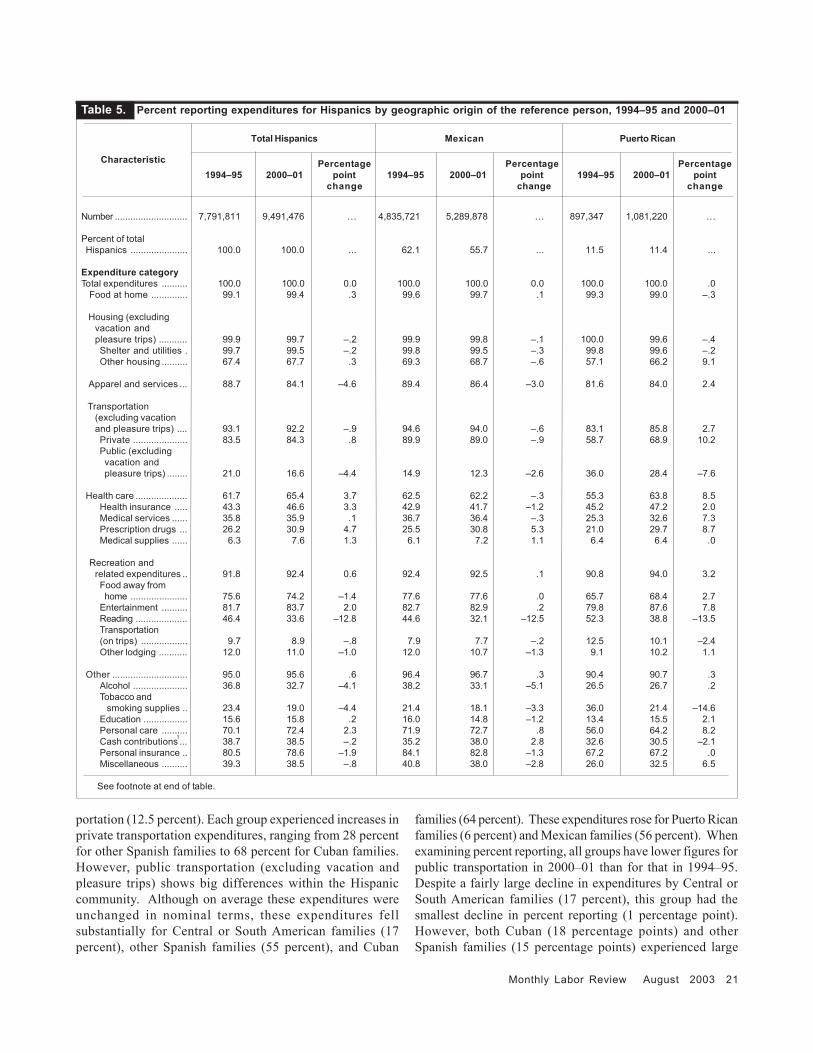
table 5, which shows the percent reporting each expenditurein 1994–95 and 2000–01, tends to support the latter hypothesis(more expensive apparel purchased) over the former (moreapparel purchased). For Puerto Rican families, the percentreporting rises slightly, from 82 percent to 84 percent. For allother Hispanic families, it falls. The smallest decline is forMexican families (3 percentage points) and the largest is forother Spanish families (15 percentage points). Given that
percent reporting is lower in most cases, this would suggestthat Hispanics are buying apparel and services less frequentlythan they used to, but that they are paying more for theapparel and services than they used to, even after adjustingfor general apparel and service price increases.
Similarly, expenditures for transportation (excludingvacation and pleasure trips) rose much more rapidly (43.1percent) for Hispanics than did the price index for trans-
Percentchange
Percentchange
Percentchange
Expenditure category
Monthly Labor Review August 2003 21
Table 5. Percent reporting expenditures for Hispanics by geographic origin of the reference person, 1994–95 and 2000–01
Total Hispanics Mexican Puerto Rican
Percentage Percentage Percentage1994–95 2000–01 point 1994–95 2000–01 point 1994–95 2000–01 point
change change change
Number ............................ 7,791,811 9,491,476 ... 4,835,721 5,289,878 ... 897,347 1,081,220 ...
Percent of totalHispanics ...................... 100.0 100.0 ... 62.1 55.7 ... 11.5 11.4 ...
Expenditure categoryTotal expenditures .......... 100.0 100.0 0.0 100.0 100.0 0.0 100.0 100.0 .0 Food at home .............. 99.1 99.4 .3 99.6 99.7 .1 99.3 99.0 –.3
Housing (excludingvacation andpleasure trips) ........... 99.9 99.7 –.2 99.9 99.8 –.1 100.0 99.6 –.4Shelter and utilities . 99.7 99.5 –.2 99.8 99.5 –.3 99.8 99.6 –.2Other housing .......... 67.4 67.7 .3 69.3 68.7 –.6 57.1 66.2 9.1
Apparel and services ... 88.7 84.1 –4.6 89.4 86.4 –3.0 81.6 84.0 2.4
Transportation(excluding vacationand pleasure trips) .... 93.1 92.2 –.9 94.6 94.0 –.6 83.1 85.8 2.7Private ..................... 83.5 84.3 .8 89.9 89.0 –.9 58.7 68.9 10.2Public (excludingvacation andpleasure trips) ........ 21.0 16.6 –4.4 14.9 12.3 –2.6 36.0 28.4 –7.6
Health care .................... 61.7 65.4 3.7 62.5 62.2 –.3 55.3 63.8 8.5Health insurance ..... 43.3 46.6 3.3 42.9 41.7 –1.2 45.2 47.2 2.0Medical services ...... 35.8 35.9 .1 36.7 36.4 –.3 25.3 32.6 7.3Prescription drugs ... 26.2 30.9 4.7 25.5 30.8 5.3 21.0 29.7 8.7Medical supplies ...... 6.3 7.6 1.3 6.1 7.2 1.1 6.4 6.4 .0
Recreation andrelated expenditures .. 91.8 92.4 0.6 92.4 92.5 .1 90.8 94.0 3.2Food away fromhome ...................... 75.6 74.2 –1.4 77.6 77.6 .0 65.7 68.4 2.7
Entertainment .......... 81.7 83.7 2.0 82.7 82.9 .2 79.8 87.6 7.8Reading .................... 46.4 33.6 –12.8 44.6 32.1 –12.5 52.3 38.8 –13.5Transportation(on trips) .................. 9.7 8.9 –.8 7.9 7.7 –.2 12.5 10.1 –2.4Other lodging ........... 12.0 11.0 –1.0 12.0 10.7 –1.3 9.1 10.2 1.1
Other ............................. 95.0 95.6 .6 96.4 96.7 .3 90.4 90.7 .3Alcohol ..................... 36.8 32.7 –4.1 38.2 33.1 –5.1 26.5 26.7 .2Tobacco and
smoking supplies .. 23.4 19.0 –4.4 21.4 18.1 –3.3 36.0 21.4 –14.6Education ................. 15.6 15.8 .2 16.0 14.8 –1.2 13.4 15.5 2.1Personal care .......... 70.1 72.4 2.3 71.9 72.7 .8 56.0 64.2 8.2Cash contributions ... 38.7 38.5 –.2 35.2 38.0 2.8 32.6 30.5 –2.1Personal insurance .. 80.5 78.6 –1.9 84.1 82.8 –1.3 67.2 67.2 .0Miscellaneous .......... 39.3 38.5 –.8 40.8 38.0 –2.8 26.0 32.5 6.5
See footnote at end of table.
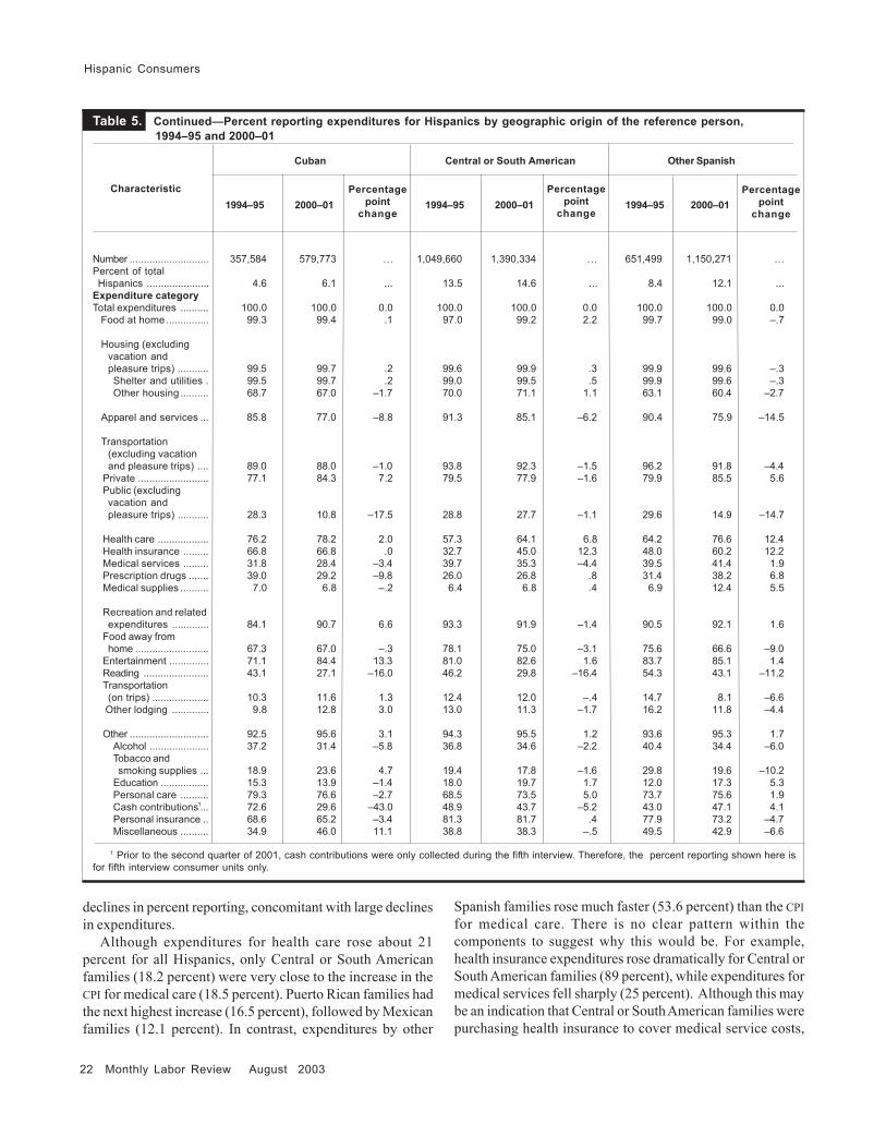
portation (12.5 percent). Each group experienced increases inprivate transportation expenditures, ranging from 28 percentfor other Spanish families to 68 percent for Cuban families.However, public transportation (excluding vacation andpleasure trips) shows big differences within the Hispaniccommunity. Although on average these expenditures wereunchanged in nominal terms, these expenditures fellsubstantially for Central or South American families (17percent), other Spanish families (55 percent), and Cuban
families (64 percent). These expenditures rose for Puerto Ricanfamilies (6 percent) and Mexican families (56 percent). Whenexamining percent reporting, all groups have lower figures forpublic transportation in 2000–01 than for that in 1994–95.Despite a fairly large decline in expenditures by Central orSouth American families (17 percent), this group had thesmallest decline in percent reporting (1 percentage point).However, both Cuban (18 percentage points) and otherSpanish families (15 percentage points) experienced large
Characteristic
1
22 Monthly Labor Review August 2003
Hispanic Consumers
Table 5. Continued—Percent reporting expenditures for Hispanics by geographic origin of the reference person, 1994–95 and 2000–01
Cuban Central or South American Other Spanish
1994–95 2000–01 1994–95 2000–01 1994–95 2000–01
Number ............................ 357,584 579,773 ... 1,049,660 1,390,334 ... 651,499 1,150,271 ...Percent of totalHispanics ...................... 4.6 6.1 ... 13.5 14.6 ... 8.4 12.1 ...
Expenditure categoryTotal expenditures .......... 100.0 100.0 0.0 100.0 100.0 0.0 100.0 100.0 0.0 Food at home ............... 99.3 99.4 .1 97.0 99.2 2.2 99.7 99.0 –.7
Housing (excludingvacation andpleasure trips) ........... 99.5 99.7 .2 99.6 99.9 .3 99.9 99.6 –.3Shelter and utilities . 99.5 99.7 .2 99.0 99.5 .5 99.9 99.6 –.3Other housing .......... 68.7 67.0 –1.7 70.0 71.1 1.1 63.1 60.4 –2.7
Apparel and services ... 85.8 77.0 –8.8 91.3 85.1 –6.2 90.4 75.9 –14.5
Transportation(excluding vacationand pleasure trips) .... 89.0 88.0 –1.0 93.8 92.3 –1.5 96.2 91.8 –4.4
Private ......................... 77.1 84.3 7.2 79.5 77.9 –1.6 79.9 85.5 5.6Public (excludingvacation andpleasure trips) ........... 28.3 10.8 –17.5 28.8 27.7 –1.1 29.6 14.9 –14.7
Health care .................. 76.2 78.2 2.0 57.3 64.1 6.8 64.2 76.6 12.4Health insurance ......... 66.8 66.8 .0 32.7 45.0 12.3 48.0 60.2 12.2Medical services ......... 31.8 28.4 –3.4 39.7 35.3 –4.4 39.5 41.4 1.9Prescription drugs ....... 39.0 29.2 –9.8 26.0 26.8 .8 31.4 38.2 6.8Medical supplies .......... 7.0 6.8 –.2 6.4 6.8 .4 6.9 12.4 5.5
Recreation and relatedexpenditures ............. 84.1 90.7 6.6 93.3 91.9 –1.4 90.5 92.1 1.6
Food away fromhome .......................... 67.3 67.0 –.3 78.1 75.0 –3.1 75.6 66.6 –9.0
Entertainment .............. 71.1 84.4 13.3 81.0 82.6 1.6 83.7 85.1 1.4Reading ....................... 43.1 27.1 –16.0 46.2 29.8 –16.4 54.3 43.1 –11.2Transportation(on trips) .................... 10.3 11.6 1.3 12.4 12.0 –.4 14.7 8.1 –6.6
Other lodging ............. 9.8 12.8 3.0 13.0 11.3 –1.7 16.2 11.8 –4.4
Other ............................ 92.5 95.6 3.1 94.3 95.5 1.2 93.6 95.3 1.7Alcohol ..................... 37.2 31.4 –5.8 36.8 34.6 –2.2 40.4 34.4 –6.0Tobacco andsmoking supplies ... 18.9 23.6 4.7 19.4 17.8 –1.6 29.8 19.6 –10.2
Education ................. 15.3 13.9 –1.4 18.0 19.7 1.7 12.0 17.3 5.3Personal care .......... 79.3 76.6 –2.7 68.5 73.5 5.0 73.7 75.6 1.9Cash contributions ... 72.6 29.6 –43.0 48.9 43.7 –5.2 43.0 47.1 4.1Personal insurance .. 68.6 65.2 –3.4 81.3 81.7 .4 77.9 73.2 –4.7Miscellaneous .......... 34.9 46.0 11.1 38.8 38.3 –.5 49.5 42.9 –6.6
1 Prior to the second quarter of 2001, cash contributions were only collected during the fifth interview. Therefore, the percent reporting shown here isfor fifth interview consumer units only.
Characteristic
declines in percent reporting, concomitant with large declinesin expenditures.
Although expenditures for health care rose about 21percent for all Hispanics, only Central or South Americanfamilies (18.2 percent) were very close to the increase in theCPI for medical care (18.5 percent). Puerto Rican families hadthe next highest increase (16.5 percent), followed by Mexicanfamilies (12.1 percent). In contrast, expenditures by other
Spanish families rose much faster (53.6 percent) than the CPIfor medical care. There is no clear pattern within thecomponents to suggest why this would be. For example,health insurance expenditures rose dramatically for Central orSouth American families (89 percent), while expenditures formedical services fell sharply (25 percent). Although this maybe an indication that Central or South American families werepurchasing health insurance to cover medical service costs,
Percentagepoint
change
Percentagepoint
change
Percentagepoint
change
1
Monthly Labor Review August 2003 23
Table 6. Average annual expenditure shares for Hispanics by geographic origin of the reference person, 1994–95 and 2000–01
Expenditure shares (in percent)
Total Puerto Central or South Other Hispanics Rican American Spanish
1994–95 2000–01 1994–95 2000–01 1994–95 2000–01 1994–95 2000–01 1994–95 2000–01 1994–95 2000–01
Number .............. 7,791,811 9,491,476 4,835,721 5,289,878 897,347 1,081,220 357,584 579,773 1,049,660 1,390,334 651,499 1,150,271Percent of totalHispanics ........ 100.0 100.0 62.1 55.7 11.5 11.4 4.6 6.1 13.5 14.6 8.4 12.1.......................... Totalexpenditures ... 100.0 100.0 100.0 100.0 100.0 100.0 100.0 100.0 100.0 100.0 100.0 100.0
Food at home . 15.1 13.3 15.3 14.0 17.5 14.2 14.1 11.1 13.7 12.3 14.2 11.9.......................... Housing(excludingvacation andpleasure trips) . 33.4 33.4 32.1 31.9 36.8 37.4 31.7 37.6 37.3 35.3 32.3 31.1Shelter andutilities ......... 29.0 28.6 27.5 27.4 32.3 32.9 26.5 32.0 33.5 30.0 28.2 26.5
Otherhousing .... 4.5 4.7 4.6 4.5 4.5 4.5 5.2 5.5 3.8 5.3 4.2 4.6
.......................... Apparel and
services ..... 5.0 4.3 5.3 4.5 4.9 4.8 3.4 3.1 4.5 4.0 4.7 4.3.......................... Transportation(excludingvacation andpleasuretrips) ................ 18.6 21.6 20.2 23.7 12.7 16.4 17.0 19.7 17.0 19.3 18.6 21.5Private ........... 18.1 21.3 20.0 23.4 11.9 15.6 16.4 19.5 16.1 18.7 17.8 21.2Public(excludingvacationand pleasuretrips) ............ .5 .4 .2 .3 .9 .8 .6 .1 .9 .6 .8 .3
.......................... Health care ....... 3.9 3.8 3.9 3.6 3.6 3.6 5.1 4.5 3.6 3.3 3.7 5.3
Healthinsurance ..... 1.9 2.0 2.0 1.8 2.2 2.1 3.3 2.7 1.1 1.7 2.0 3.0
Medicalservices ....... 1.5 1.2 1.5 1.2 .9 .9 1.2 1.2 2.1 1.2 1.3 1.3
Prescriptiondrugs ........... .3 .5 .3 .5 .3 .5 .5 .5 .2 .3 .3 .6
Medicalsupplies ....... .1 .2 .1 .1 .2 .1 .1 .1 .1 .1 .1 .3
Recreationand relatedexpenditures ... 8.9 8.8 8.5 8.6 9.4 9.4 10.4 9.1 9.2 8.5 10.0 9.2Food awayfrom home ... 3.6 3.5 3.6 3.7 3.2 3.3 4.2 3.1 3.8 3.4 3.3 3.5
Entertain-ment ............. 3.8 3.8 3.7 3.8 4.0 4.1 4.2 3.8 3.4 3.2 4.5 4.2
Reading ......... .3 .2 .3 .2 .4 .2 .4 .2 .4 .2 .4 .3Transportation(on trips) ...... .8 .7 .5 .5 1.1 .9 1.0 1.1 1.0 1.1 1.2 .6
Other lodging .5 .6 .4 .4 .7 .9 .6 .9 .6 .7 .6 .7.......................... Other ................. 15.1 15.7 14.7 14.8 15.2 14.8 18.4 15.8 14.8 17.9 16.5 17.5
Alcohol ........... .7 .7 .8 .7 .5 .6 .9 .7 .7 .7 .6 .7Tobacco andsmokingsupplies ....... .6 .6 .5 .5 1.3 1.0 .5 .7 .4 .4 .7 .7
Education ...... 1.1 1.1 .7 .7 1.8 1.3 1.7 1.1 1.9 1.7 1.1 1.7Personal care . .8 .8 .8 .7 .8 .8 1.3 .8 .9 .8 .9 .9Cash contri-butions ......... 1.7 2.2 1.6 1.9 1.3 1.8 3.8 1.6 1.5 3.9 1.8 2.0
Personal insurance .... 8.1 8.7 8.0 8.7 7.8 8.1 7.8 8.7 7.7 8.5 9.9 9.7
Miscellane-ous ............... 2.1 1.6 2.3 1.5 1.7 1.2 2.4 2.3 1.7 1.8 1.5 1.8
Mexican Cuban Expenditurecategory
24 Monthly Labor Review August 2003
Hispanic Consumers
apparently, they did not achieve as much success inprescription drug coverage, as these expenditures rose 69percent—more than the increase for Puerto Rican families (54percent) or Cuban families (20 percent). In contrast,expenditures for health insurance rose 61 percent for otherSpanish families, while expenditures for medical services rose13 percent, and prescription drug expenditures rose 100percent for these consumer units. The percent reporting doesnot add much clarity to the situation. The percent reportinghealth insurance was relatively stable for Mexican (1-percentage point decrease), Puerto Rican (2-percentage pointincrease), and Cuban families (no change). The percentreporting rose substantially for Central or South Americanand other Spanish families (12 percentage points in each case).However, percent reporting medical services decreased forCentral or South American families (4 percentage points),while it increased for other Spanish families (2 percentagepoints).
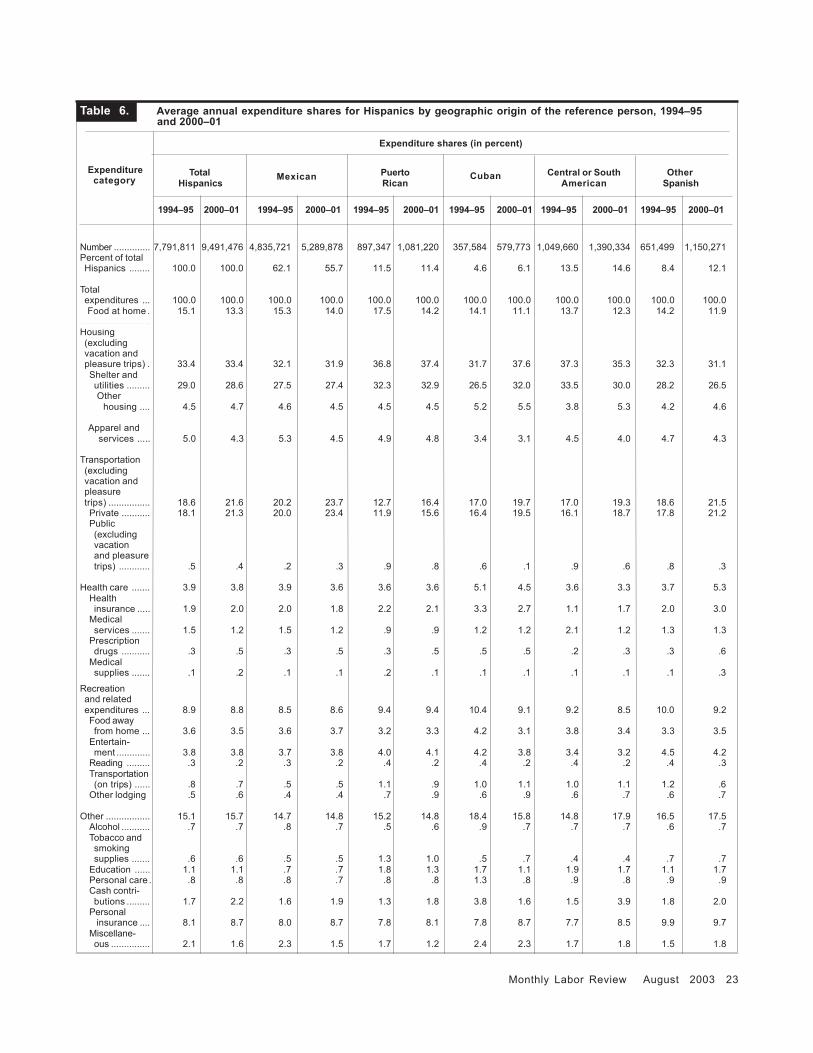
Expenditure shares. Another way to analyze expenditurepatterns is to examine expenditure shares, or the proportionof total expenditures allocated to specific goods and servicesby the average family. Expenditure shares control for pricechanges, at least to some extent; if expenditures for a specificitem increase over time, it may be due to increased con-sumption or increased prices, as stated before. However, ifall prices double, and quantities purchased remain the same,then expenditures will double but shares will remain the same.As evidenced earlier in this article, inflation is rarely “pure”—that is, affecting all items in the same way. Still, expenditureshares provide an idea of how consumption is changing in arelative framework. Regardless of price levels, differences inshares may indicate different consumption patterns for groups.One method of analyzing these changes was developed byPrussian economist Ernst Engel in the 19th century. Accordingto Engel’s Proposition of 1857, as income increases, theproportion of total expenditures allocated to food decreases.Also, Engel found that shares allocated to housing and apparelstay roughly constant as income increases, while sharesallocated for “luxury goods” increase.15 Engel’s findings canbe used to analyze economic standing of different groupswithin the same time period, or the same group across timeperiods. For example, if the share of total expendituresallocated to food has decreased for a specific group over time,presumably, it is not because they are eating less food, butrather because prices for food have fallen, or incomes haverisen (or both). Either way, this leaves more income for thegroup to allocate to other expenditures, and allows them toincrease consumption or savings without giving up any food.
According to the type of analysis Engel performed,Hispanics are better off in 2000–01 than they were in 1994–95. As a group, the share of total expenditures allocated tofood at home declined from 15 percent to 13 percent (table6). The smallest change in percentage points was for Mexican
families, whose share decreased from 15.3 percent of totalexpenditures to 14.0 percent. The largest change in percentagepoints was for Puerto Ricans, whose share decreased from17.5 percent to 14.2 percent.
Consistent with Engel’s findings, the shares allocated toapparel and services and housing were stable for all groups,with the exception of Cuban families. For these consumers,the share of total expenditures allocated to housing rosesubstantially, from 32 percent to 38 percent. This was nearlyall accounted for by an increase in the share allocated toshelter and utilities, which rose from 27 percent to 32 percent.Similarly, expenditures for health care were stable for allgroups; the largest change was for other Spanish families, inwhich case the share rose from 3.7 percent to 5.3 percent oftotal expenditures. Perhaps surprisingly, shares for recreationand related expenditures also held steady. This is not onlytrue at the aggregate level, but also for all subcomponents forall groups.
Finally, according to Engel’s analysis, transportationappears to be a luxury good, as shares for all groups increasenotably. For Hispanics in general, the share rose from 19percent to 22 percent of total expenditures. Of course, thisexpenditure category is dominated by private transportation.Again, for each group, private transportation shares rose. Thesmallest increase was for Central or South American families(16.1 to 18.7 percent), while the largest was for Puerto Ricanfamilies (11.9 to 15.6 percent).
Regression analysis
As described, differences in expenditure patterns areobserved across Hispanic groups. Some of these differencesmay be due to differences in tastes and preferences acrossthe groups. However, table 2 shows that there are alsodemographic differences across groups. Differences inincome, age, or other characteristics can also influenceexpenditure patterns. To help discern what differences maybe due to demographic differences and what differences maybe due to underlying differences in tastes and preferences bygeographic origin, regression analysis is used. As describedin the previous work that this study updates,16 regressionanalysis allows the user to estimate how (in this case)differences in geographic origin might be related todifferences in expenditures, ceteris paribus (that is, giventhat all other characteristics are held constant). As with theprevious work, major expenditure categories (food at home,shelter and utilities,17 apparel and services, transportationexcluding vacation and pleasure trips, and recreation andrelated expenditures) are examined using ordinary leastsquares regression. The “other” expenditures category isomitted from the analysis, despite constituting a substantialshare of total expenditures, because it is composed of aneclectic mixture of goods and services. It is not clear what themeaning of the results of this regression would be at the
Monthly Labor Review August 2003 25
Table 7. Standardized results: Marginal propensity to expend (MPE) and permanent income elasticity by Hispanic group and expenditure category, 1994–95 and 2000–01
Mexican Puerto Rican Cuban
1994–95 2000–01 1994–95 2000–01 1994–95 2000–01 1994–95 2000–01 1994–95 2000–01
Total expenditures ..................................... $24,911 $30,651 $24,911 $30,651 $24,911 $30,651 $24,911 $30,651 $24,911 $30,651Food at home .......................................... 3,761 4,063 3,761 4,063 3,761 4,063 3,761 4,063 3,761 4,063
Marginal propensity to expend ........... 0.034 10.040 20.055 0.044 0.045 0.046 20.061 10.040 0.038 0.041Permanent income elasticity .............. 0.228 0.299 0.363 0.334 0.299 0.344 0.406 0.303 0.252 0.310
................................................................ Shelter and utilities ................................ 7,216 8,779 7,216 8,779 7,216 8,779 7,216 8,779 7,216 8,779
Marginal propensity to expend ........... 0.145 10.151 20.189 20.201 0.120 1,20.186 20.183 20.171 0.164 0.149Permanent income elasticity .............. 0.501 0.526 0.654 0.703 0.416 0.651 0.633 0.596 0.531 0.520
................................................................... Apparel and services ............................. 1,246 1,322 1,246 1,322 1,246 1,322 1,246 1,322 1,246 1,322
Marginal propensity to expend ........... 0.073 0.057 20.093 0.065 20.049 0.057 0.069 0.060 0.086 20.070Permanent income elasticity .............. 1.467 1.319 1.862 1.517 0.976 1.316 1.373 1.387 1.727 1.633
.................................................................. Transportation (excluding vacationand pleasure trips) ............................... 4,632 6,629 4,632 6,629 4,632 6,629 4,632 6,629 4,632 6,629Marginal propensity to expend ........... 0.268 0.320 20.386 20.403 20.341 20.405 0.254 0.343 20.168 2.258Permanent income elasticity .............. 1.443 1.481 2.074 1.865 1.833 1.870 1.367 1.586 0.903 1.191
................................................................... Recreation and related expenditures ..... 2,219 2,684 2,219 2,684 2,219 2,684 2,219 2,684 2,219 2,684
Marginal propensity to expend ........... 0.143 0.144 0.157 0.129 20.184 0.159 0.142 0.140 0.150 0.148Permanent income elasticity .............. 1.611 1.641 1.766 1.478 2.063 1.814 1.593 1.602 1.689 1.695
2 Income coefficient is statistically significantly different from Mexicanconsumers at the 90-percent confidence level; see table 8 for more information.
1 Income coefficient is statistically significantly different from 1994–95 atthe 90-percent confidence level; see table 8 for more information.
aggregate level, and the individual components are tooinfrequently reported to warrant separate analysis.
Description of variables. In addition to the expendituresdescribed (that is, the dependent variables), severalindependent variables are used in these regressions. Mostare common to all regressions. Consistent with the previouswork, these variables include: total expenditures, age (andage squared) of reference person, number of adults (andnumber squared), number of children18 (and number squared),and dummy variables describing the reference person’s familytype (single person, husband and wife only, single parent, orother family), region of residence (Northeast, Midwest, orWest), degree of urbanization (rural), education (less thanhigh school graduate, some college, or college graduate), andworking status (self-employed, retired, or not working forreasons other than retirement). The “omitted” categories forthese dummy variables include: husband and wife withchildren (family type), South (region of residence), urban(degree of urbanization), high school graduate (education),and wage and salary earner (working status). These variablesare omitted, as is traditional when dummy variables areemployed, to avoid perfect multicollinearity.
In updating the previous work, two new binary variablesare added: Black and other race. (The omitted category isWhite.) In the previous work, race did not differ substantiallyacross Hispanic groups. Only two—Central or SouthAmerican (7.4 percent) and other Spanish (10.4 percent) hadsubstantially more than 5 percent reporting “Black” for race
of the reference person. (Cuban families had 5.3 percentreporting, but they were the smallest Hispanic group in 1994–95.) For “other race,” all groups reported less than 2 percent,and two groups (Cuban and other Spanish) had no reports forreference person of “other race.” However, as mentionedearlier, the sample is larger in 2000–01 than 1994–95, thusproviding more observations for families whose referenceperson is Black or “other race.” Additionally, the percentagethat report Black for race of reference person has increasedfor all Hispanic groups except other Spanish (for whom itdeclined), and each group has at least some reports of “otherrace.” Because the Hispanic groups are now less homogenousby race, and because homogeneity may continue to decreasein the future, race is now added to the regression analysis.The 1994–95 regression results reported in this work includethis variable as well as the 2000–01 results.
In addition, a few independent variables are included only inselected regressions. For example, the housing regressioncontains dummy variables describing housing tenure (owned withno mortgage or renter; owned with mortgage is omitted) andcontinuous variables describing size of dwelling (number ofrooms, bedrooms, bathrooms, and half-baths).19 The regressionsfor transportation and recreation and related expenditures alsocontain variables describing number of automobiles and othervehicles owned by the consumer unit. These variables areselectively included because in each case, they will clearly affectexpenditures for the dependent variable under study, but do notnecessarily directly affect other expenditures. (For example,number of bedrooms will clearly affect housing expenditures,
Expenditure category
Central or SouthAmerican
OtherSpanish
26 Monthly Labor Review August 2003
Hispanic Consumers
but not food at home expenditures.)Also important is the inclusion of total expenditures as a
proxy for permanent income. This is done for both theoreticaland empirical reasons. Theoretically, consumers do not makeexpenditure decisions based only on income received today(that is, current income), but also on income they expect toreceive in the future. This theory, proposed by MiltonFriedman, is known to economists as the “permanent incomehypothesis.”20 But there are empirical reasons for usingpermanent income as well. For example, because “permanent”income incorporates expectations of future earnings, there maybe less variability in the relationship between expenditures and“permanent” income than “current” income.21 Furthermore,current income is not necessarily reported in full by allfamilies, even by so-called complete reporters. Removing“incomplete” reporters reduces sample size, and not even in
Table 8. Statistical significance of coefficient changes over time by Hispanic group and selected expenditure categories, 1994–95 and 2000–01
Puerto Central or South OtherRican American Spanish
1994–95 2000–01 1994–95 2000–01 1994–95 2000–01 1994–95 2000–01 1994–95 2000–01
Total expenditures ...................................... $24,911 $30,651 $24,911 $30,651 $24,911 $30,651 $24,911 $30,651 $24,911 $30,651 Food at home .......................................... 3,761 4,063 3,761 4,063 3,761 4,063 3,761 4,063 3,761 4,063
Different intercept than Mexicans ........ ... ... 99 (1) (1) (1) 99 (1) (1) (1)
Different MPE than Mexicans ................ ... ... 99 (1) (1) (1) 99 (1) (1) (1)
Different intercept than owngroup 1994–95 .................................... ... 95 ... (1) ... (1) ... 95 ... (1)
Different MPE than 1994–95 .................. ... 99 ... (1) ... (1) ... 90 ... (1)
................................................................... Shelter and utilities ................................. 7,216 8,779 7,216 8,779 7,216 8,779 7,216 8,779 7,216 8,779
Different intercept than Mexicans ........ ... ... 99 99 (1) 99 99 90 (1) (1)
Different MPE than Mexicans ................ ... ... 99 99 (1) 99 99 95 (1) (1)
Different intercept than owngroup 1994–95 .................................... ... (1) ... (1) ... 99 ... (1) ... (1)
Different MPE than 1994–95 ................. ... 95 ... (1) ... 99 ... (1) ... (1)
................................................................... Apparel and services .............................. 1,246 1,322 1,246 1,322 1,246 1,322 1,246 1,322 1,246 1,322
Different intercept than Mexicans ....... ... ... 95 (1) (1) (1) (1) (1) (1) 95Different MPE than Mexicans ............... ... ... 90 (1) 90 (1) (1) (1) (1) 95Different intercept than owngroup 1994–95 .................................... ... (1) ... (1) ... (1) ... (1) ... (1)
Different MPE than 1994–95 ................. ... (1) ... (1) ... (1) ... (1) ... (1)
................................................................... Transportation (excluding vacationand pleasure trips) ................................. 4,632 6,629 4,632 6,629 4,632 6,629 4,632 6,629 4,632 6,629Different intercept than Mexicans ....... ... ... 99 99 95 99 (1) (1) 99 99Different MPE than Mexicans ............... ... ... 99 99 95 99 (1) (1) 99 99Different intercept than owngroup 1994–95 .................................... ... (1) ... (1) ... (1) ... 90 ... 90
Different MPE than 1994–95 ................. ... (1) ... (1) ... (1) ... (1) ... (1)
Recreation and related expenditures ...... 2,219 2,684 2,219 2,684 2,219 2,684 2,219 2,684 2,219 2,684Different intercept than Mexicans ....... ... ... (1) (1) 95 (1) (1) (1) (1) (1)
Different MPE than Mexicans ............... ... ... (1) (1) 95 (1) (1) (1) (1) (1)
Different intercept than owngroup 1994–95 .................................... ... 95 ... (1) ... (1) ... (1) ... (1)
Different MPE than 1994–95 ................. ... (1) ... (1) ... (1) ... (1) ... (1)
1 The difference is not statistically significant at the 90-percent confidence level.
Expenditure categoryMexican Cuban
a random fashion, because incomplete reporters are notrandomly distributed throughout the CE sample.22
Furthermore, following a general trend in income reporting,the percentage of Hispanic consumer units classified ascomplete income reporters was lower in 2000–01 than in 1994–95, especially for Cuban, Central or South American, and otherSpanish families (table 2). For all these reasons, totalexpenditures are used as a proxy for permanent income. (Forconvenience, the term “income” will be used henceforth tomean “permanent income.”)
Model specification. The goal of the regressions is toobtain parameter estimates that can be used to calculate themarginal propensity to expend (MPE) for different goods andservices for each Hispanic group in 2000–01, and to comparethese results both intra-temporally (for example, Puerto Rican
Monthly Labor Review August 2003 27
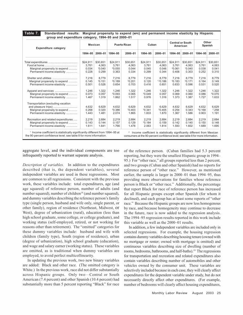
families to Mexican families in 2000–01) and inter-temporally(for example, Puerto Rican families in 2000–01 to PuertoRican families in 1994–95). The MPE’s are then used tocalculate income elasticity for each good or service to seewhether or not there are differences in expenditure patternsamong Hispanics of different geographic origin. Similarly,following the previous work, these elasticities are estimatedfor each Hispanic group by using its own mean permanentincome (“unadjusted” estimation) or by using the averagepermanent income for the sample as a whole (“standardized”estimation) in cases where permanent income is needed toestimate these factors.
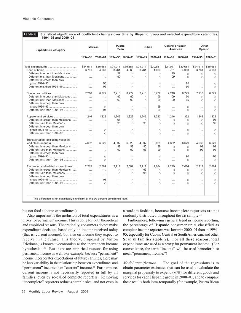
To achieve these goals accurately, Box-Cox transformationsare performed on both the dependent variables and the incomevariables in each of the equations. These transformations are usedto reduce heteroscedasticity. (See appendix for details.) Forconsistency, the same transformations are applied to the 2000–01 data as were applied to the 1994–95 data in the previous work.Because of the Box-Cox transformations, parameter estimatesin most of the models do not have any immediately interpretableintuitive meaning. Therefore, for the reader’s convenience,important measures that are derived from these parameterestimates (such as the MPE’s and income elasticities,described subsequently) are presented in table 7. Table 8describes whether the income parameters are different acrossgeographic origin within each time period, and whether theincome parameters have changed over time within eachgeographic origin.
The model, then, is specified as follows:
Y* = αm + αmT + ∑α iDi + ∑α iDiT + βmI + βmIT + ∑βiDiI +∑βiDiIT + βjXj + βjXjT + e
where
Y* is the (Box-Cox transformation of the) dependentvariable;
αm is the intercept of the regression equation;T is a dummy variable describing the time period for the
interview (0 for 1994–95; 1 for 2000–01);α i are parameter estimates;Di are dummy variables describing geographic origin for
non-Mexican Hispanics;βm,βi are parameter estimates for the income variable;I is permanent income (i.e., total expenditures);β j is a vector of parameter estimates for various
independent variables;Xj is a vector of independent variables;e is the error of the regression.
This specification allows relationships for all variables todiffer by geographic origin as well as over time, and forstatistical tests to be performed to ascertain whether or not
observed differences are statistically significant. In the 1994–95 data, t-tests are sufficient to distinguish whether parameterestimates differ statistically from the reference group to thegroup in question. For changes over time, F-tests are used.23
Because Mexicans are the largest segment of the Hispanicpopulation, it is with reference to them that statisticallysignificant differences are examined. While it is possible totest each group against each other (for example, are Cubansstatistically significantly different from Puerto Ricans), suchcomparisons would be cumbersome with five groups,especially when comparing across years. Because the mainpoint of this section is to test whether Hispanics arehomogeneous or not in 2000–01, and whether expenditurepatterns have changed over time for each group, thisspecification provides sufficient information.
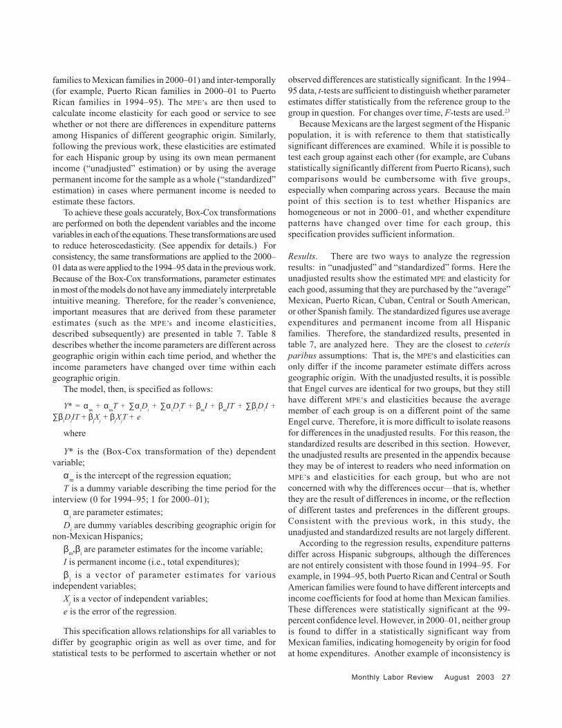
Results. There are two ways to analyze the regressionresults: in “unadjusted” and “standardized” forms. Here theunadjusted results show the estimated MPE and elasticity foreach good, assuming that they are purchased by the “average”Mexican, Puerto Rican, Cuban, Central or South American,or other Spanish family. The standardized figures use averageexpenditures and permanent income from all Hispanicfamilies. Therefore, the standardized results, presented intable 7, are analyzed here. They are the closest to ceterisparibus assumptions: That is, the MPE's and elasticities canonly differ if the income parameter estimate differs acrossgeographic origin. With the unadjusted results, it is possiblethat Engel curves are identical for two groups, but they stillhave different MPE’s and elasticities because the averagemember of each group is on a different point of the sameEngel curve. Therefore, it is more difficult to isolate reasonsfor differences in the unadjusted results. For this reason, thestandardized results are described in this section. However,the unadjusted results are presented in the appendix becausethey may be of interest to readers who need information onMPE’s and elasticities for each group, but who are notconcerned with why the differences occur—that is, whetherthey are the result of differences in income, or the reflectionof different tastes and preferences in the different groups.Consistent with the previous work, in this study, theunadjusted and standardized results are not largely different.
According to the regression results, expenditure patternsdiffer across Hispanic subgroups, although the differencesare not entirely consistent with those found in 1994–95. Forexample, in 1994–95, both Puerto Rican and Central or SouthAmerican families were found to have different intercepts andincome coefficients for food at home than Mexican families.These differences were statistically significant at the 99-percent confidence level. However, in 2000–01, neither groupis found to differ in a statistically significant way fromMexican families, indicating homogeneity by origin for foodat home expenditures. Another example of inconsistency is
28 Monthly Labor Review August 2003
Hispanic Consumers
that other Spanish families were not statisticallysignificantly different from Mexican families in their appareland service expenditures in 1994–95, but they are differentin 2000–01. In some cases, though, the differences areconsistent across time. For example, Puerto Rican familiesare found to be significantly different from Mexican familiesin their transportation expenditures; in each time periodtested, both the intercept and income coefficient differstatistically at the 99-percent confidence level. And forCuban families, the difference has become moresignificant—rising from 95 percent confidence in 1994–95to 99 percent confidence in 2000–01 for both the interceptand income coefficient.
Perhaps of more interest is whether changes within groupshave taken place over time. That is, do Mexican families (andall other groups) in 2000–01 still have the same intercept andincome coefficients that they had for food at home (or otherexpenditures) in 1994–95? In many cases, changes are observedover time for one or more groups of Hispanic consumers.
For food at home, Mexican consumers have experienced achange in both the intercept and slope of their Engel curves.The change in the slope means that MPE, and therefore,elasticity, have changed over time. The MPE has risen from 3cents to 4 cents, and the elasticity has risen from 0.23 to 0.30.Central or South American families have had the oppositeexperience—the MPE has fallen from 6 cents to 4 cents, andelasticity has fallen from 0.41 to 0.30.
For shelter and utilities, the coefficient for income forMexican families increased by a statistically significantamount, but it had little effect on the estimated MPE orelasticity. However, for Cuban families, both changedsubstantially. The MPE rose from 12 cents to 19 cents; theelasticity rose from 0.42 to 0.65. This may be related to thechange in housing tenure observed for Cuban families overthe study period.24
For the remaining expenditures, no income coefficientchanges are significant at the 95-percent confidence level.Although in some cases there appear to be notable changesover time (for example, for Cuban families, the apparel andservice elasticity rises from 0.98 to 1.32) the change is notstatistically significant, and may be observed by chance.
Summary and conclusions
Previous literature has shown that not only does ethnicityaccount for substantial variation in consumer expenditures, ithas shown that these differences can occur among subgroupsof particular ethnicities. In particular, while many researcherstreat “Hispanics” as homogenous, previous work finds thatthere is substantial variation in expenditure patterns byHispanics of different geographic origin.
This work shows that the Hispanic population is worthrevisiting. The percentage of the population accounted for
by Hispanic consumers continues to increase at a substantialpace. In addition, the composition of the Hispanic populationhas changed even in the few years since the previous workwas published. For example, although Mexican families arestill the majority of Hispanic families, they account for asmaller portion of the total in 2000–01 than in 1994–95, inlarge part ceding ground to families of “other Spanish” origin.Given these changes, it is important to see whetherexpenditure patterns have changed at the aggregate level and,if so, whether or not the changes are due solely to changes incomposition of the Hispanic population, or are at least in partcaused by underlying changes in tastes and preferences of thegroups under study. (These changes could be caused bychanges in the groups themselves; for example, immigrantsarriving from Mexico between 1994–95 and 2000–01 mighthave different tastes and preferences than those who were hereprior to 1994. Unfortunately, because no data on length ofresidency in the United States are collected by the ConsumerExpenditure Survey, it is not possible to precisely identify thecause of the differences.)
Some demographic characteristics, such as age ofreference person, have not changed much over the studyperiod for Hispanics. However, others, such as educationalattainment, appear to have changed. Some of these changesmay explain higher levels of total expenditures in 2000–01,which for Mexican, Cuban, and Central or South Americanfamilies rose faster than inflation. For other Spanish families,total expenditures also increased, but at a slower rate thaninflation. Despite these changes, though, most Hispanicfamilies in the aggregate account for approximately theirpopulation share of total expenditures in the economy. (Forexample, Mexicans account for 56 percent of Hispanicconsumer units and 54 percent of total consumerexpenditures by Hispanics.)
Analysis of expenditure shares indicates that Hispanics, ingeneral, are spending a smaller proportion of their dollars onfood at home, which means they have a larger share to spendon other goods and services. Given that food at home is anecessity good, this suggests that Hispanics are a bit betteroff economically in 2000–01 than they were in 1994–95.
Finally, regression analysis is performed to estimate whetherchanges observed in expenditures are due to changes in incomeor other similar factors, or to changes in underlying preferences.As with the earlier study, substantial variation is observed acrossgeographic origins. However, over time, only a few changes haveoccurred. As explained in the main text, it is difficult to controlcompletely for price changes in performing these analyses, sothese results should be interpreted cautiously.
This work shows that Hispanic consumers continue to bean important segment of total consumer expenditures in theUnited States. It also shows that expenditure patterns continueto differ by geographic origin, at the same time geographicorigin is changing within the Hispanic community. Given
Monthly Labor Review August 2003 29
these changing characteristics and the increasing proportionof the population for which the Hispanic community accounts,it is important to continue to monitor these groups to obtaina better understanding of the patterns in consumer spendingand predicting what shapes they may take in the future.
ACKNOWLEDGMENT: The author gratefully acknowledges Dr. Bárbara J.Robles, University of Texas at Austin, for suggesting that recent, rapidchanges in the Hispanic community warrant a new look at expenditurepatterns for these consumers.
1 U.S. Bureau of the Census, Statistical Abstract of the United States:2001, p. 17, table 15, available on the Internet at: http://www.census.gov/prod/2002pubs/01statab/pop.pdf.
2 More information on consumer spending by Hispanics, is availableonand http://www.bls.gov/cex/2000/Standard/tenracar.pdf. However,comparable tables of consumer spending by Hispanics are not available atthis site prior to 1994.
3 For examples, see Janet Wagner and Horacio Soberon-Ferrar,“The Effect of Ethnicity on Selected Household Expenditures,” TheSocial Science Journal, February 1990, pp. 181–98; and Geoffrey D.Paulin, “A growing market: expenditures by Hispanic consumers,”Monthly Labor Review, March 1998, pp. 3–21.
4 Paulin, “A growing market.”
5 Geoffrey D. Paulin, “Variation in Food Purchases: A Study of Inter-Ethnic and Intra-Ethnic Group Patterns Involving the HispanicCommunity,” Family and Consumer Sciences Research Journal, vol. 29,no. 4, June 2001, pp. 336–381.
6 A consumer unit is defined as members of a household related byblood, marriage, adoption, or other legal arrangement; a single personliving alone or sharing a household with others but who is financiallyindependent; or two or more persons living together who shareresponsibility for at least two out of three major types of expenses— food,housing, and other expenses. In this article, the terms consumer unit,family, and household are used interchangeably for convenience.
7 These data describing consumer units are obtained from theInterview component of the Consumer Expenditure Survey. Theweights for this survey are updated periodically using data obtainedfrom the Census Bureau. In addition to using later information incomputing the revised weights, the methodology for constructingthe weights changed for processing the 1997 and later data. (SeeBLS Handbook of Methods, Chapter 16, http://www.bls.gov/opub/hom/homch16_c.htm . ) For these reasons alone, one mightexpect to see differences in outcomes for 1994–95 data, whichwere processed using the old weighting scheme, and the 2000–01data, processed using the revised weighting scheme. In addition,the sample size increased in 1999, as described subsequently in thetext. However, data from the U.S. Bureau of the Census (based onthe Current Population Survey) also shows that the Hispaniccommunity is changing. The results, in fact, are similar to thoseshown in table 1, at least for overall growth rates. Using population,rather than consumer unit, figures, the Census data show that thenon-Hispanic population increased 6 percent from 1995 to 2000,compared with 19 percent for the Hispanic population. They alsoshow that each Hispanic ethnic group increased faster than thenon-Hispanic population: 21 percent for Mexican origin; 8 percentfor Puerto Rican origin; 12 percent for Cuban origin; 29 percentfor Central or South American origin; and 7 percent for otherSpanish origin. (For 1995 data, see U.S. Bureau of the Census,Statistical Abstract of the United States: 1996, p. 51, table 53,
http://www.census.gov/prod/2/gen/96statab/pop.pdf; for 2000 data,see U.S. Bureau of the Census, Statistical Abstract of the United States:2001, p. 43, table 41, http://www.census.gov/prod/2002pubs/01statab/pop.pdf) Some of the differences between the ConsumerExpenditure Survey and Census data may lie in the fact that the first setis based on numbers of consumer units, and the second set is based onindividual members of the population; if one community has a largeinflux of single-person immigrants, for example, and the establishedcommunity is comprised of multi-member families, the number ofconsumer units may increase dramatically, while the population for thegroup does not rise so rapidly. Additionally, there are differences inmethodologies for calculating the figures used by the different sources.(For example, the Consumer Expenditure Survey weights are notcomputed using ethnic origin, but the Current Population Survey weightsdo use ethnic origin; see BLS Handbook of Methods, Chapter 1, http://www.bls.gov/opub/hom/homch1_g.htm.) Nevertheless, each showsthat the Hispanic population is changing dramatically, and indicatesusefulness in examining these groups once again.
8 Paulin, “A growing market.”9 A report describing the 1998–99 survey results indicates that the
“Interview survey collects detailed data on an estimated 60 percent to70 percent of total household expenditures. Global estimates, that is,expense patterns for a 3-month period, are obtained for food andother selected items, accounting for an additional 20 percent to 25percent of total expenditures.” See Consumer Expenditure Survey1998–99, Report 955 (Bureau of Labor Statistics, November 2001),p. 272.
10 The first person identified when the respondent is asked who isresponsible for owning or renting the home. In this study, the referenceperson is assumed to be the parent in all cases.
11 “Mexican” origin includes reference persons identified asMexican; Mexican-American; and Chicano. “Central or SouthAmerican” origin may include reference persons from Brazil, FrenchGuyana, or other areas where the official language is not Spanish. TheConsumer Expenditure Survey only asks whether the reference personis of “Central or South American” origin, and does not allow for finerdistinctions. Similarly, “other Spanish” could include persons withfamilial ties to Spain, Caribbean islands other than Puerto Rico orCuba (such as the Dominican Republic), or other areas. It is importantto note these differences, because changes over time in these groups(Central and South American as well as other Spanish) may be due tochanges in the underlying composition of these groups, which are notdetectable in the Consumer Expenditure Survey.
12 In general, complete income reporters are defined as consumerunits for which the respondent reports at least one major source ofincome for the consumer unit, such as wages and salaries, self-employment income, or Social Security income. However, evencomplete income reporters do not necessarily provide a full accountingof income from all sources.
13 Data from the U.S. Immigration and Naturalization Serviceconfirm that patterns of immigration have changed for CentralAmericans. According to data presented in the U.S. Statistical Abstracts(1996, table 8; and 2002, table 7) immigration from Central Americarose from 39,900 in 1994 to 66,400 in 2000; an increase of 66 percent.By far, the largest increase is for immigrants from Nicaragua. In 1994,approximately 5,300 immigrants arrived from this country. In 2000,the number increased to 24,000; an increase of 353 percent. In addition,the proportion of immigrants from Central America for whichNicaraguans accounted rose from 13 percent to 36 percent—that is,from fewer than 1 in 7 to more than 1 in 3. Immigrants from ElSalvador, who had accounted for the largest proportion—44 percent—in 1994, dropped to second place in 2000—34 percent. Nevertheless,the only group for which the number of immigrants actually declined
Notes
30 Monthly Labor Review August 2003
Hispanic Consumers
was for Panama. There were 2,400 immigrants from this country in1994 compared to 1,800 in 2000.
Although the data for South American immigrants are limited onthese tables, they show that total immigration from South Americarose 18 percent over this time, from 47,400 immigrants in 1994 to56,100 in 2000. (When immigrants from Brazil and Guyana—the twonon-Spanish speaking countries for which data are available—areexcluded, the increase is 23 percent.) Data for other Spanish are evenless available, although immigration from the Dominican Republicdeclined substantially, from 51,200 in 1994 to 17,500 in 2000.
For more information on immigration patterns from these areas,see the U.S. Statistical Abstracts.
14 Paulin, “Variation in Food Purchases,” 2001.
15 Louis Phlips, Applied Consumption Analysis (Amsterdam,Elsevier Science Publishers B.V.; distributed in the U.S. and Canada byElsevier Science Publishing Company, Inc. of New York, NY), p. 103.
16 Paulin, “A growing market.”
17 Shelter and utilities is analyzed instead of total housing becauseshelter (largely, rent and mortgage interest payments) and utilitiescontitutes the basic expenditures most families would incur on arecurring basis.
18 In this case, children are defined as persons under 18 years old. Inthe Consumer Expenditure Survey, they are defined as the offspring ofthe reference person. It is possible that a person under 18 is not theoffspring of the reference person. This may be because the referenceperson is the grandparent, aunt or uncle, or some other relative of theperson under 18. It may also be that the person under 18 is thereference person—for example, a 17-year-old college student mightbe included in the sample. By the same token, number of adults isascertained by subtracting persons under 18 from total family size.Therefore, in the case of the 17-year-old college student, the consumerunit could have no adults and one child.
19 There are slightly fewer degrees of freedom for the housingregressions because variables related to size of dwelling are occasionally
missing in the Consumer Expenditure Survey data. However, thenumber of missing values is small, and the pattern of missingness ispresumed to be random, so the omission of these observations shouldnot cause any problems in the analysis.
20 Milton Friedman, A Theory of the Consumption Function(Princeton, search, 1957), p. 221.
21 Suppose, for example, that one family consistently earns$20,000 per year, and another one usually earns $15,000, but forsome reason received an unexpected $5,000 in income during the pastyear. Even though both families earned $20,000 in “current” income,they may have very different spending patterns. Note that each willhave different “permanent” incomes, because the family receivingthe extra transitory income ($5,000) will realize that this is a onetime only event, and adjust spending accordingly.
22 For a detailed discussion of “complete” and “incomplete”reporters, see Geoffrey D. Paulin and David L. Ferraro , “Imputingincome in the Consumer Expenditure Survey,” Monthly Labor Review,December 1994, pp. 23–31.
23 Additional tables containing specific results, such as parameterestimates, t-statistics, and F-statistics are available on the Internet at:http://www.bls.gov/cex/csxart.htm or upon request to the author:[email protected].
24 The percentage of Cuban families sampled who report “owning witha mortgage” increases substantially from 1994–95 to 2000–01, while thepercentage reporting renting their homes decreases substantially. Inprevious work, Geoffrey D. Paulin finds that homeowners and rentershave different tastes and preferences, even when other characteristics aretaken into account. This work finds that homeowners have a lower MPEthan renters for primary housing and related services, but in that study,primary housing and related services includes household operations andhouse furnishings and equipment in addition to shelter and utilities, whichare studied separately in this article. Therefore, it is difficult to say preciselywhether the change in MPE is a direct result of the difference in percentreporting renting versus owning, or due to other factors. See Geoffrey D.Paulin, “A Comparison of Consumer Expenditures by Housing Tenure,”The Journal of Consumer Affairs, Summer 1995, pp. 164–198, especially,pp. 174–75.
APPENDIX: Notes on methodology
Box-Cox transformations. The two most importantvariables (aside from ethnicity) considered in this section areexpenditures and income. However, neither of these is oftenfound to have a normal distribution,1 a problem that can causebiased regression results. One solution is to transform thesedata so that they are approximately normally distributed. Onemethod that has been used with expenditure data is the Box-Cox transformation.2 Perhaps the most frequently citedversion is as follows:
Y* = (Yλ - 1)/λwhereY* is the transformed version of the variableY is expenditures for a specific good or service (forexample, food at home or apparel)λ is a parameter.
This version of the equation is most useful in de-monstrating two special cases for the value of λ . On the onehand, if λ is one, then no transformation of the independentvariable is necessary. (The net result is that Y* equals Y - 1,and subtracting a constant from each observation of Y willnot affect the distribution.) On the other hand, if λ approacheszero, then Y* is approximately equal to the natural log of Y.
Although this specification is useful for deriving the valueof Y* when λ approaches zero, it does not yield an intuitiveinterpretation when λ takes on any other value.3 However, onthe same page of the original article on which they describethis specification, G.E.P. Box and D.R. Cox point out that thisequation can be simplified to:
Y* = Yλ
This leads to a simple interpretation of both λ and the
Monthly Labor Review August 2003 31
equation as a whole. For example, if λ is found to be ½, thenthe transformed variable is simply the square root of Y. In theregression, then, each value of the dependent value is replacedby its square root, and the regression is performed in theusual way. (Note that at least for the special case where λequals one, it is even easier to see that no transformation isnecessary; Y* equals Y in this case.)
The obvious question raised is how one calculates thevalue of λ. Conventionally, this is done by trial and error.Several values for λ are used, and whichever λ yields themodel with the lowest mean square error is the selected value.However, this method is extremely time consuming, and nearlyimpossible when one considers that there are two variables(expenditures AND income) that are being trans-formed. Inthis study λ is estimated through a maximum likelihoodprocedure described by Stuart Scott and Daniel J. Rope, whospecifically study transformations of Consumer ExpenditureSurvey data.4 The results of this procedure are shown in thefollowing text tabulation:
Expenditure Optimal valuefor λ
Food at home .............................................. 0.250Shelter and utilities ..................................... .250Apparel and services .................................. .125Transportation (excluding vacation
and pleasure trips) ................................ .000Recreation and related expenditures .......... .125Health care .................................................. .125
Marginal propensity to expend. One of the most importantresults that can be derived from the regressions presented isthe marginal propensity to expend (MPE).5 This term is definedas the percentage of an additional dollar the family wouldspend on a specific good if given an additional dollar. TheMPE is equal to the slope of the Engel curve (that is,expenditures as a function of income for each good orservice), and is a critical component of elasticity; each of theelasticities shown in table 5 of the text are derived from themarginal propensity to expend money for the same good.
In most literature, the MPE is referred to as the “marginalpropensity to consume” (MPC). In the previous work, in fact, theterm “MPC” was used. The reason for the difference interminology comes from the inter-temporal comparisons. Theusual meaning of the term MPC is the change in quantitydemanded given a unit increase in income. It can also mean thechange in expenditure given a unit increase in income, as noted.However, this is only true assuming prices are constant. Toillustrate, suppose that a person regularly purchases apples bythe pound. The expenditure for apples can be shown to be:
X = PQWhereX is the expenditure on apples;P is the price per pound for apples;
Q is the number of pounds of apples purchased.Suppose further that expenditures are a linear function of
income:
X = a + bI.
According to this equation, if income (I) rises by one dollar,expenditures (X) will increase by b cents. Because the priceper pound is fixed for all consumers who shop at the samestore (that is, it is not related to income), the only way that Xcan change in response to an increase in I is because Qchanges in response to an increase in I. That is, the higherthe income, the more pounds of apples the customerpurchases.
During the time frames under study (1994–95 and 2000–01) price changes were fairly small, in general. However,even if year-to-year changes are small, over time, they canadd up to large changes in prices across the periods (that is,when comparing 1994–95 to 2000–01). Note that even if I andQ stay the same, X could rise over time simply because P risesover time. (It is even possible for X to rise if P rises by a largerpercentage than Q declines.) If price changes affected allgoods in exactly the same way, it would be easy to control forthese changes when comparing MPEs. However, as describedin the text, the different goods and services comparedexperienced different price changes over time; in fact,although most prices rose, prices for apparel and servicesdeclined from 1994–95 to 2000–01. None of the price increasesstudied exactly matched the increase in overall prices.Therefore, relative prices of goods and services will differ overthe periods. For example, as noted, prices for apparel and servicesdeclined while total prices increased. Therefore, apparel andservices are relatively less expensive in 2000–01 than in 1994–95.Similarly, prices for transportation rose at a slower rate (12.5percent) than all prices (16.2 percent). Although actual priceswere higher in 2000–01 for transportation than they were in1994–95, relative to other goods and services, transportationcost less in 1994–95 than in 2000–01. And because prices formedical care rose faster (18.5 percent) than other prices,medical care was relatively more expensive in 2000–01 than in1994–95, although its relative increase (that is, its increasecompared with other price increases) is not nearly so large asits actual price increase (the aforementioned 18.5 percent).Given that relative prices are different in these time periods,then even given the same income across years, consumerswill allocate the dollars differently (for example, they mightpurchase more apparel and services in 2000–01 than in 1994–95). Even if permanent income is price-adjusted by the changein total prices, different allocations will occur if the pricechange for the good under study is different than the changein total prices.6 That is, because of the change in relativeprices, the MPE for each good changes. The reason is thatthe change in relative prices changes the Engel curve thatdescribes the consumer’s expenditures.7
One way to correct for the change in relative prices is toadjust both permanent income by the change in overall prices,and adjust the specific good (that is, food at home) by the change
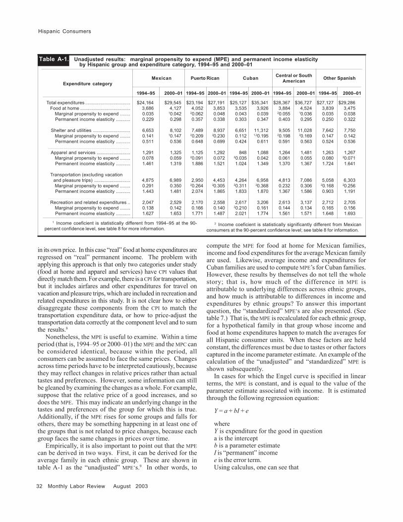
32 Monthly Labor Review August 2003
Hispanic Consumers
Table A-1. Unadjusted results: marginal propensity to expend (MPE) and permanent income elasticity by Hispanic group and expenditure category, 1994–95 and 2000–01
Mexican Puerto Rican Cuban Other Spanish
1994–95 2000–01 1994–95 2000–01 1994–95 2000–01 1994–95 2000–01 1994–95 2000–01
Total expenditures ................................... $24,164 $29,545 $23,194 $27,191 $25,127 $35,341 $28,367 $36,727 $27,127 $29,286 Food at home ....................................... 3,686 4,127 4,052 3,853 3,535 3,926 3,884 4,524 3,839 3,475 Marginal propensity to expend ........ 0.035 10.042 20.062 0.048 0.043 0.039 20.055 10.036 0.035 0.038 Permanent income elasticity ........... 0.229 0.298 0.357 0.338 0.303 0.347 0.403 0.295 0.250 0.322...............................................................
Shelter and utilities ............................. 6,653 8,102 7,489 8,937 6,651 11,312 9,505 11,028 7,642 7,750 Marginal propensity to expend ........ 0.141 10.147 20.209 20.230 0.112 1,20.195 20.198 20.169 0.147 0.142 Permanent income elasticity ........... 0.511 0.536 0.648 0.699 0.424 0.611 0.591 0.563 0.524 0.536...............................................................
Apparel and services .......................... 1,291 1,325 1,125 1,292 848 1,088 1,264 1,481 1,263 1,267 Marginal propensity to expend ........ 0.078 0.059 20.091 0.072 20.035 0.042 0.061 0.055 0.080 20.071 Permanent income elasticity ........... 1.461 1.319 1.886 1.521 1.024 1.349 1.370 1.367 1.724 1.641...............................................................
Transportation (excluding vacationand pleasure trips) ............................ 4,875 6,989 2,950 4,453 4,264 6,958 4,813 7,086 5,058 6,303
Marginal propensity to expend ........ 0.291 0.350 20.264 20.305 20.311 20.368 0.232 0.306 20.168 20.256 Permanent income elasticity ........... 1.443 1.481 2.074 1.865 1.833 1.870 1.367 1.586 0.903 1.191...............................................................
Recreation and related expenditures .. 2,047 2,529 2,170 2,558 2,617 3,206 2,613 3,137 2,712 2,705 Marginal propensity to expend ........ 0.138 0.142 0.166 0.140 20.210 0.161 0.144 0.134 0.165 0.156 Permanent income elasticity ........... 1.627 1.653 1.771 1.487 2.021 1.774 1.561 1.571 1.648 1.693
Central or SouthAmericanExpenditure category
in its own price. In this case “real” food at home expenditures areregressed on “real” permanent income. The problem withapplying this approach is that only two categories under study(food at home and apparel and services) have CPI values thatdirectly match them. For example, there is a CPI for transportation,but it includes airfares and other expenditures for travel onvacation and pleasure trips, which are included in recreation andrelated expenditures in this study. It is not clear how to eitherdisaggregate these components from the CPI to match thetransportation expenditure data, or how to price-adjust thetransportation data correctly at the component level and to sumthe results.8
Nonetheless, the MPE is useful to examine. Within a timeperiod (that is, 1994–95 or 2000–01) the MPE and the MPC canbe considered identical, because within the period, allconsumers can be assumed to face the same prices. Changesacross time periods have to be interpreted cautiously, becausethey may reflect changes in relative prices rather than actualtastes and preferences. However, some information can stillbe gleaned by examining the changes as a whole. For example,suppose that the relative price of a good increases, and sodoes the MPE. This may indicate an underlying change in thetastes and preferences of the group for which this is true.Additionally, if the MPE rises for some groups and falls forothers, there may be something happening in at least one ofthe groups that is not related to price changes, because eachgroup faces the same changes in prices over time.
Empirically, it is also important to point out that the MPEcan be derived in two ways. First, it can be derived for theaverage family in each ethnic group. These are shown intable A-1 as the “unadjusted” MPE’s.9 In other words, to
compute the MPE for food at home for Mexican families,income and food expenditures for the average Mexican familyare used. Likewise, average income and expenditures forCuban families are used to compute MPE’s for Cuban families.However, these results by themselves do not tell the wholestory; that is, how much of the difference in MPE isattributable to underlying differences across ethnic groups,and how much is attributable to differences in income andexpenditures by ethnic groups? To answer this importantquestion, the “standardized” MPE’s are also presented. (Seetable 7.) That is, the MPE is recalculated for each ethnic group,for a hypothetical family in that group whose income andfood at home expenditures happen to match the averages forall Hispanic consumer units. When these factors are heldconstant, the differences must be due to tastes or other factorscaptured in the income parameter estimate. An example of thecalculation of the “unadjusted” and “standardized” MPE isshown subsequently.
In cases for which the Engel curve is specified in linearterms, the MPE is constant, and is equal to the value of theparameter estimate associated with income. It is estimatedthrough the following regression equation:
Y = a + bI + e
whereY is expenditure for the good in questiona is the interceptb is a parameter estimateI is “permanent” incomee is the error term.Using calculus, one can see that
1 Income coeficient is statistically different from 1994–95 at the 90-percent confidence level, see table 8 for more information.
2 Income coeficient is statistically significantly different from Mexicanconsumers at the 90-percent confidence level; see table 8 for information.
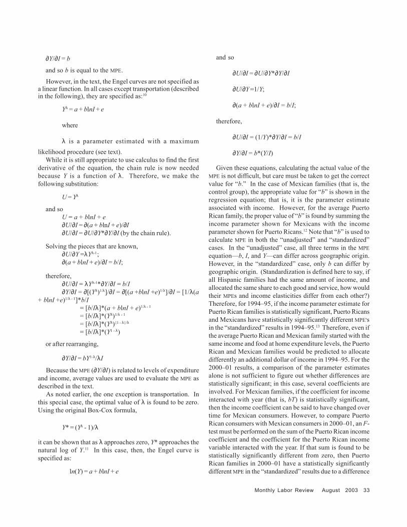
Monthly Labor Review August 2003 33
∂Y/∂I = b
and so b is equal to the MPE.
However, in the text, the Engel curves are not specified asa linear function. In all cases except transportation (describedin the following), they are specified as:10
Yλ = a + blnI + e
where
λ is a parameter estimated with a maximumlikelihood procedure (see text).
While it is still appropriate to use calculus to find the firstderivative of the equation, the chain rule is now neededbecause Y is a function of λ . Therefore, we make thefollowing substitution:
U = Yλ
and soU = a + blnI + e∂U/∂I = ∂(a + blnI + e)/∂I∂U/∂I = ∂U/∂Y*∂Y/∂I (by the chain rule).
Solving the pieces that are known,∂U/∂Y =λYλ-1;∂(a + blnI + e)/∂I = b/I;
therefore,∂U/∂I = λYλ-1*∂Y/∂I = b/I∂Y/∂I = ∂[(Yλ)1/λ]/∂I = ∂[(a +blnI +e)1/λ]/∂I = [1/λ(a
+ blnI +e)1/λ - 1]*b/I= [b/Iλ]*(a + blnI + e)1/λ - 1
= [b/Iλ]*(Yλ)1/λ - 1
= [b/Iλ]*(Yλ){1 - λ}/λ
= [b/Iλ]*(Y1 - λ)
or after rearranging,
∂Y/∂I = bY1-λ/λI
Because the MPE (∂Y/∂I) is related to levels of expenditureand income, average values are used to evaluate the MPE asdescribed in the text.
As noted earlier, the one exception is transportation. Inthis special case, the optimal value of λ is found to be zero.Using the original Box-Cox formula,
Y* = (Yλ - 1)/λ
it can be shown that as λ approaches zero, Y* approaches thenatural log of Y.11 In this case, then, the Engel curve isspecified as:
ln(Y) = a + blnI + e
and so
∂U/∂I = ∂U/∂Y*∂Y/∂I
∂U/∂Y =1/Y;
∂(a + blnI + e)/∂I = b/I;
therefore,
∂U/∂I = (1/Y)*∂Y/∂I = b/I
∂Y/∂I = b*(Y/I)
Given these equations, calculating the actual value of theMPE is not difficult, but care must be taken to get the correctvalue for “b.” In the case of Mexican families (that is, thecontrol group), the appropriate value for “b” is shown in theregression equation; that is, it is the parameter estimateassociated with income. However, for the average PuertoRican family, the proper value of “b” is found by summing theincome parameter shown for Mexicans with the incomeparameter shown for Puerto Ricans.12 Note that “b” is used tocalculate MPE in both the “unadjusted” and “standardized”cases. In the “unadjusted” case, all three terms in the MPEequation—b, I, and Y—can differ across geographic origin.However, in the “standardized” case, only b can differ bygeographic origin. (Standardization is defined here to say, ifall Hispanic families had the same amount of income, andallocated the same share to each good and service, how wouldtheir MPEs and income elasticities differ from each other?)Therefore, for 1994–95, if the income parameter estimate forPuerto Rican families is statistically significant, Puerto Ricansand Mexicans have statistically significantly different MPE'sin the “standardized” results in 1994–95.13 Therefore, even ifthe average Puerto Rican and Mexican family started with thesame income and food at home expenditure levels, the PuertoRican and Mexican families would be predicted to allocatedifferently an additional dollar of income in 1994–95. For the2000–01 results, a comparison of the parameter estimatesalone is not sufficient to figure out whether differences arestatistically significant; in this case, several coefficients areinvolved. For Mexican families, if the coefficient for incomeinteracted with year (that is, bT) is statistically significant,then the income coefficient can be said to have changed overtime for Mexican consumers. However, to compare PuertoRican consumers with Mexican consumers in 2000–01, an F-test must be performed on the sum of the Puerto Rican incomecoefficient and the coefficient for the Puerto Rican incomevariable interacted with the year. If that sum is found to bestatistically significantly different from zero, then PuertoRican families in 2000–01 have a statistically significantlydifferent MPE in the “standardized” results due to a difference
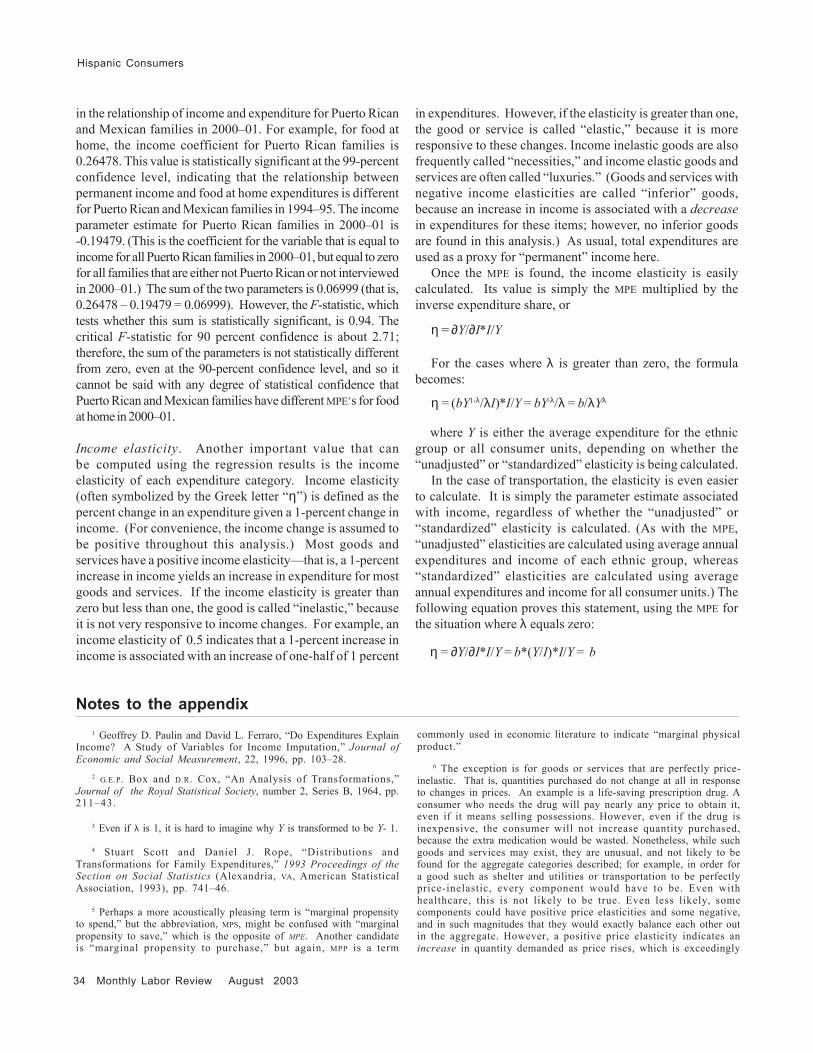
34 Monthly Labor Review August 2003
Hispanic Consumers
in the relationship of income and expenditure for Puerto Ricanand Mexican families in 2000–01. For example, for food athome, the income coefficient for Puerto Rican families is0.26478. This value is statistically significant at the 99-percentconfidence level, indicating that the relationship betweenpermanent income and food at home expenditures is differentfor Puerto Rican and Mexican families in 1994–95. The incomeparameter estimate for Puerto Rican families in 2000–01 is-0.19479. (This is the coefficient for the variable that is equal toincome for all Puerto Rican families in 2000–01, but equal to zerofor all families that are either not Puerto Rican or not interviewedin 2000–01.) The sum of the two parameters is 0.06999 (that is,0.26478 – 0.19479 = 0.06999). However, the F-statistic, whichtests whether this sum is statistically significant, is 0.94. Thecritical F-statistic for 90 percent confidence is about 2.71;therefore, the sum of the parameters is not statistically differentfrom zero, even at the 90-percent confidence level, and so itcannot be said with any degree of statistical confidence thatPuerto Rican and Mexican families have different MPE’s for foodat home in 2000–01.
Income elasticity. Another important value that canbe computed using the regression results is the incomeelasticity of each expenditure category. Income elasticity(often symbolized by the Greek letter “η”) is defined as thepercent change in an expenditure given a 1-percent change inincome. (For convenience, the income change is assumed tobe positive throughout this analysis.) Most goods andservices have a positive income elasticity—that is, a 1-percentincrease in income yields an increase in expenditure for mostgoods and services. If the income elasticity is greater thanzero but less than one, the good is called “inelastic,” becauseit is not very responsive to income changes. For example, anincome elasticity of 0.5 indicates that a 1-percent increase inincome is associated with an increase of one-half of 1 percent
in expenditures. However, if the elasticity is greater than one,the good or service is called “elastic,” because it is moreresponsive to these changes. Income inelastic goods are alsofrequently called “necessities,” and income elastic goods andservices are often called “luxuries.” (Goods and services withnegative income elasticities are called “inferior” goods,because an increase in income is associated with a decreasein expenditures for these items; however, no inferior goodsare found in this analysis.) As usual, total expenditures areused as a proxy for “permanent” income here.
Once the MPE is found, the income elasticity is easilycalculated. Its value is simply the MPE multiplied by theinverse expenditure share, or
η = ∂Y/∂I*I/Y
For the cases where λ is greater than zero, the formulabecomes:
η = (bY1-λ/λI)*I/Y = bY-λ/λ = b/λYλ
where Y is either the average expenditure for the ethnicgroup or all consumer units, depending on whether the“unadjusted” or “standardized” elasticity is being calculated.
In the case of transportation, the elasticity is even easierto calculate. It is simply the parameter estimate associatedwith income, regardless of whether the “unadjusted” or“standardized” elasticity is calculated. (As with the MPE,“unadjusted” elasticities are calculated using average annualexpenditures and income of each ethnic group, whereas“standardized” elasticities are calculated using averageannual expenditures and income for all consumer units.) Thefollowing equation proves this statement, using the MPE forthe situation where λ equals zero:
η = ∂Y/∂I*I/Y = b*(Y/I)*I/Y = b
Notes to the appendix1 Geoffrey D. Paulin and David L. Ferraro, “Do Expenditures Explain
Income? A Study of Variables for Income Imputation,” Journal ofEconomic and Social Measurement, 22, 1996, pp. 103–28.
2 G.E.P. Box and D.R. Cox, “An Analysis of Transformations,”Journal of the Royal Statistical Society, number 2, Series B, 1964, pp.211–43.
3 Even if λ is 1, it is hard to imagine why Y is transformed to be Y- 1.
4 Stuart Scott and Daniel J. Rope, “Distributions andTransformations for Family Expenditures,” 1993 Proceedings of theSection on Social Statistics (Alexandria, VA, American StatisticalAssociation, 1993), pp. 741–46.
5 Perhaps a more acoustically pleasing term is “marginal propensityto spend,” but the abbreviation, MPS, might be confused with “marginalpropensity to save,” which is the opposite of MPE. Another candidateis “marginal propensity to purchase,” but again, MPP is a term
commonly used in economic literature to indicate “marginal physicalproduct.”
6 The exception is for goods or services that are perfectly price-inelastic. That is, quantities purchased do not change at all in responseto changes in prices. An example is a life-saving prescription drug. Aconsumer who needs the drug will pay nearly any price to obtain it,even if it means selling possessions. However, even if the drug isinexpensive, the consumer will not increase quantity purchased,because the extra medication would be wasted. Nonetheless, while suchgoods and services may exist, they are unusual, and not likely to befound for the aggregate categories described; for example, in order fora good such as shelter and utilities or transportation to be perfectlyprice-inelastic, every component would have to be. Even withhealthcare, this is not likely to be true. Even less likely, somecomponents could have positive price elasticities and some negative,and in such magnitudes that they would exactly balance each other outin the aggregate. However, a positive price elasticity indicates anincrease in quantity demanded as price rises, which is exceedingly
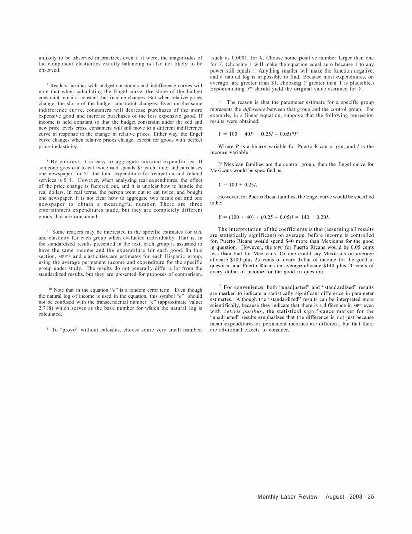
Monthly Labor Review August 2003 35
unlikely to be observed in practice; even if it were, the magnitudes ofthe component elasticities exactly balancing is also not likely to beobserved.
7 Readers familiar with budget constraints and indifference curves willnote that when calculating the Engel curve, the slope of the budgetconstraint remains constant, but income changes. But when relative priceschange, the slope of the budget constraint changes. Even on the sameindifference curve, consumers will decrease purchases of the moreexpensive good and increase purchases of the less expensive good. Ifincome is held constant so that the budget constraint under the old andnew price levels cross, consumers will still move to a different indifferencecurve in response to the change in relative prices. Either way, the Engelcurve changes when relative prices change, except for goods with perfectprice-inelasticity.
8 By contrast, it is easy to aggregate nominal expenditures: Ifsomeone goes out to eat twice and spends $5 each time, and purchasesone newspaper for $1, the total expenditure for recreation and relatedservices is $11. However, when analyzing real expenditures, the effectof the price change is factored out, and it is unclear how to handle thereal dollars. In real terms, the person went out to eat twice, and boughtone newspaper. It is not clear how to aggregate two meals out and onenewspaper to obtain a meaningful number. There are threeentertainment expenditures made, but they are completely differentgoods that are consumed.
9 Some readers may be interested in the specific estimates for MPEand elasticity for each group when evaluated individually. That is, inthe standardized results presented in the text, each group is assumed tohave the same income and the expenditure for each good. In thissection, MPE’s and elasticities are estimates for each Hispanic group,using the average permanent income and expenditure for the specificgroup under study. The results do not generally differ a lot from thestandardized results, but they are presented for purposes of comparison.
10 Note that in the equation “e” is a random error term. Even thoughthe natural log of income is used in the equation, this symbol “e” shouldnot be confused with the transcendental number “e” (approximate value:2.718) which serves as the base number for which the natural log iscalculated.
11 To “prove” without calculus, choose some very small number,
such as 0.0001, for λ. Choose some positive number larger than onefor Y. (choosing 1 will make the equation equal zero because 1 to anypower still equals 1. Anything smaller will make the function negative,and a natural log is impossible to find. Because most expenditures, onaverage, are greater than $1, choosing Y greater than 1 is plausible.)Exponentiating Y* should yield the original value assumed for Y.
12 The reason is that the parameter estimate for a specific grouprepresents the difference between that group and the control group. Forexample, in a linear equation, suppose that the following regressionresults were obtained:
Y = 100 + 40P + 0.25I – 0.05I*P
Where P is a binary variable for Puerto Rican origin, and I is theincome variable.
If Mexican families are the control group, then the Engel curve forMexicans would be specified as:
Y = 100 + 0.25I.
However, for Puerto Rican families, the Engel curve would be specifiedto be:
Y = (100 + 40) + (0.25 – 0.05)I = 140 + 0.20I.
The interpretation of the coefficients is that (assuming all resultsare statistically significant) on average, before income is controlledfor, Puerto Ricans would spend $40 more than Mexicans for the goodin question. However, the MPC for Puerto Ricans would be 0.05 centsless than that for Mexicans. Or one could say Mexicans on averageallocate $100 plus 25 cents of every dollar of income for the good inquestion, and Puerto Ricans on average allocate $140 plus 20 cents ofevery dollar of income for the good in question.
13 For convenience, both “unadjusted” and “standardized” resultsare marked to indicate a statistically significant difference in parameterestimates. Although the “standardized” results can be interpreted morescientifically, because they indicate that there is a difference in MPE evenwith ceteris paribus , the statistical significance marker for the“unadjusted” results emphasizes that the difference is not just becausemean expenditures or permanent incomes are different, but that thereare additional effects to consider.