Embed Size (px)
Citation preview

1/05 Utilities • 7-1
7. Utilities
I. Tide (Water Level) Corrections There are several ways to incorporate your Tide Corrections into your data set. These include the following: • Log the data from a telemetry tide gauge in real time in the
SURVEY program. • Manually enter the corrections in real time in the SURVEY
program. • Create a Tide Correction file using:
▪ harmonic predictions in the HARMONIC PREDICTION program.
▪ predicted high-low water times in the MANUAL TIDES program.
▪ actual tide levels and times in the MANUAL TIDES program.
The resulting Tide files can be graphed and displayed from HYPACK® MAX by right clicking on the Tide File in the Project Files list and selecting Graph.
Details about logging data from real time telemetry gauges and manually entering the Tide Corrections are contained in the SURVEY section of this manual. The following sections will deal with creating Tide Correction files from harmonic predictions, high-low water times and heights, and tide observations.
The important thing to remember in all of these methods is that the Tide Correction is going to be added to the raw sounding. Tide Corrections relate raw soundings to the chart (low water) datum. Since you normally want to remove the water column above the sounding datum, the overwhelming majority of the time your tide corrections will be negative numbers! The HARMONIC PREDICTION program takes care of this automatically. You have to make some mental adjustments when entering tidal heights in the MANUAL TIDES program. • When creating a tide file for depth mode, enter tide values as
negative numbers. • When creating a tide file for elevation mode, enter tide values as
positive numbers. Units are according to those selected in the GEODETIC PARAMETERS program (feet or meters).

7-2 • Utilities 1/05
Any sounding collected before the first time of your *.TID file will get the value of that first time. Any sounding collected after the last time of your *.TID file will get the value of that last time.
If you read tides from a telemetry gauge or if you manually entered them while collecting survey data in the SURVEY program, you can skip this section. When you start the single beam and multibeam EDITORS, it will have all of the information it needs to compute tide corrections for each sounding.
A. Harmonic Tidal Predictions We don’t intend to teach you about Harmonic Tidal Predictions and harmonic constituents. All we want to do is show you how to create a Tide Correction file (*.TID) using the HARMONIC PREDICTION program.
The routines in this program are taken from the British Admiralty publication N.R.203. It uses combined constituent data for M2, S2, O1, and K1. This means that the minor constituents of them are combined into these four values. The harmonic constituents published by the French hydrographic authorities take a slightly different approach, so they won’t give the correct answer if you plug them into these formulae.
In order to compute a harmonic tidal prediction, you need the following information: • The harmonic constituents for the desired port • The day factors (0000H) for the day in question • The day factors (0000H) for the next day
It needs the day factors. for both days in order to perform an interpolation throughout the day. All of these constituents and factors are published in the British Admiralty publication N.R.203. It comes out every year and is divided into three volumes. One is for the Atlantic Ocean, Caribbean, and Mediterranean. The second is for the Pacific Ocean. The third is for the Indian Ocean ports. You can buy these from your Admiralty chart agent.
1) Running the Harmonic Tides Program 1. Start the program from the tides icon or by clicking
PROCESSING-TIDES-HARMONIC TIDES. The Harmonic Tides dialog will appear.
2. Enter the necessary information. ▪ The Date for Prediction, Site for Prediction, Mean Level and
Seasonal Correction come from the Port Factor page. ▪ Enter the Harmonic Constituents for the port. ▪ Enter the day factors (0000H) for the day of the prediction ▪ Enter the day factors (0000H) for the day after the prediction
3. Save the input data by clicking [Save Tide Ref].

1/05 Utilities • 7-3
4. Click on [Compute And Graph]. A graph of your tide corrections over a 24 hour period will appear. You can return to the spreadsheet to recheck your data by clicking [Exit] or continue on.
5. Save your corrections by clicking on [Save To *.TID]. You will be asked for a name for the Tide Correction file. Give it a name you can remember, one that reminds you both of the area and the day for which the corrections are made.
In the input dialog: [Get Last Reference] reloads the last saved data.
[New Prediction] presents an empty dialog.
In the graph dialog:
[Print Graph] sends the graph display to the Windows® default printer.
[Print Corrections] sends a copy of your entries in the spreadsheet and a listing of time ranges and their predicted tide corrections over the specified time range.
2) Harmonic Tides Example Example: Harmonic Tides
Perform a harmonic prediction for the port of Boston, using the following information. Date: 24 Sept 97 Site: Boston, MA Mean Level: 1.85 Seasonal Level: 0.00
Item M2-g M2-H S2-g S2-H K1-g K1-H O1-g O1-H Port 158 0.72 221 0.32 56 0.11 331. 0.08
24 Sept. 331 1.01 232 0.05 6 1.12 221 1.20
25 Sept. 359 1.02 233 0.84 7 1.12 179 1.21
Solution: 6. Start the program. Click on PROCESSING-TIDES-
HARMONIC TIDE. The spreadsheet will appear. 7. Enter the information into the spreadsheet.

7-4 • Utilities 1/05
Harmonic Tides Spreadsheet
8. Save the input data by clicking [Save Tide Ref]. 9. Click on [Compute and Graph]. The program will calculate a
predicted tidal value for every minute of the day. The information will be drawn to a graph as shown below.
The Predicted Tide Graph in the Harmonic TIDES Program.
10. Click on [Save To *.TID] and name your Tide Correction file.
Give it a name that reminds you of both the site and the day of the correction. In our case we have named it BOS0924.TID. The program will automatically assign the extension .TID to any name you give, and save the file in the project directory.
The key thing to remember about harmonic tides is that they are only predictions. Meteorological effects can cause drastic changes to the actual water levels.

1/05 Utilities • 7-5
B. Tide Corrections from High-Low Water Times and Heights Another way of creating a file of predicted tide corrections is to use the capabilities of the MANUAL TIDES program.
1) Running the Manual Tides Program with High-Low Water Times and Heights
1. Open the MANUAL TIDES program by clicking PROCESSING-TIDES-MANUAL TIDES. The Manual tides dialog will appear.
2. Enter the time and height of the last tide of the previous day, preceded by a minus sign (“-“). This is a flag to the program that it is from the previous day. Enter the corresponding height.
3. Enter the time and heights of the day for which the prediction is being made.
4. Enter the time and height of the first high-water of the next day. Preceded this time with a plus sign (“+”) to designate that it is from the next day.
5. Click on Min-Max. This tells the program to use the high water-low water prediction algorithm developed by NOAA. The program calculates a tide height for every minute of the day. The results are graphed on the right.
6. Save your file by clicking on FILE-SAVE and giving your file a name. Make sure the name is chosen to remind you of both the site and the day of the correction. It will be saved with the default *.TID extension, to your project directory.
Note: If you are using the NOAA tide book and you are working in depth mode, you need to place a minus sign in front of all of your height entries. For example, if the NOAA book shows a high tide that is 5.6’ above gauge, you need to remove 5.6’ from the water column. You, therefore, have to enter -5.6’ in HYPACK® MAX.
2) Manual Tides Program Example with High-Low Water Times and Heights
Example: Creating Tide Files using MANUAL TIDES
Create a Tide Correction (*.TID) file using the following information from the NOAA book.
Day Time Height November 24 23:15 3.20 November 25 05:05 0.20 10:59 3.70 16:48 0.50 22:35 3.20 November 26 04:32 0.30
Solution:

7-6 • Utilities 1/05
1. Open the MANUAL TIDES program and enter the data so it looks like the figure below. Notice the time from November 24 is entered with a minus sign since it is from the previous day. The time from November 26 is entered with a plus sign, since it is from the next day. All of the NOAA heights have a minus sign placed in front of them because we want to remove the water from the sounding.
2. Click on Min-Max. Your graph will be drawn as shown on the right side of the following figure.
Entering data for High-Low Waters
3. Save your file by clicking on FILE-SAVE and save the file to
“BOS_1125.TID”.
C. Tide Corrections with Manual Observations The MANUAL TIDES program is used to create a Tide Correction file (*.TID) from manually observed tides. The tides are then applied to the RAW data files in the single beam or multibeam editing programs to obtain edited data files. As stated a couple of times, your tide corrections will almost always be negative numbers because HYPACK® MAX is going to add your tide correction to the raw sounding.
1) Running the Manual Tides Program with Manual Observations 1. Open the MANUAL TIDES program by clicking
PROCESSING-TIDES-MANUAL TIDE or from the TIDES icon.
2. Enter the time and tide correction pairs in the grid. A handy feature with the MANUAL TIDES program is the AutoTime feature. Enter a Starting Time and Ending Time, along with a time increment, click [OK] and the program will automatically fill the time column with the requested times.

1/05 Utilities • 7-7
Auto-time Dialog
3. Select either the Linear or the Spline method. The Spline
method fits the curve through your data points.
Note: You need at least five points to run the spline algorithm. 4. Save your tide corrections. The MANUAL TIDES program
saves your table of data to a *.TDX file and your tide corrections to a *.TID file. This allows you to later retrieve the tide table should there be any questions about what values were used.
2) Manual Tides Program Example with Manual Observations Example: Manual Tides
During the day, our crackerjack tide staff reader made the following readings of times and gauge heights.
Time Gauge Height 08:00 3.20 09:00 2.80 09:55 2.10 11:00 2.00 11:45 2.10 13:00 2.30 14:00 2.70 14:45 4.20 Your mission is to make a *.TID file named “FAKEDATA.TID”, using a straight-line interpolation between the points. Once you’re done, click on [Spline] to see what it looks like.
Solution: 1. Open the MANUAL TIDES program by clicking
PROCESSING-TIDES-MANUAL TIDE or from the TIDES icon..
2. Enter the values as given above. Since we are given the height of the water above the gauge zeros, we have to enter the correction values as negative numbers.
3. Click on [Linear] and the points will be connected with a straight line.

7-8 • Utilities 1/05
Tide Data with Linear Interpolation
4. Save the file. Click on FILE-SAVE and enter the file name. It will save the table data to the FAKEDATA.TDK FILE and the tide corrections to the FAKEDATA.TID file.
5. Click on [Spline]. Your graph should now look like the following figure.
Tide Data with Spline Interpolation
D. Importing NOAA Tide Data to Manual Tides Program Historical water level data can be obtained from NOAA's website and imported into the Manual Tides Program.
Tide data can be obtained from http://www.co-ops.nos.noaa.gov. 1. Down load the pertinent data from NOAA's website.
a. Follow the links for "Verified/Historical Water Level Data". b. Select the "YYYY/MM/DD HH:MM" date output format. c. Select the location and dates appropriate to your survey. d. Click [View Data] located near the bottom of the page and
the information will load in your browser window.

1/05 Utilities • 7-9
e. Select FILE-SAVE AS in the Microsoft Internet Explorer or Netscape Navigator menu and name your file, changing the file extension to "txt".
2. In the MANUAL TIDES program, click [NOAA] and select the downloaded text file. A dialog will appear with a list of dates found in the file.
3. Select a date in the window (must appear highlighted not just outlined) and click [OK] (or use a double click when selecting the date). Tide corrections are inverted from the NOAA file for compatability with our software.
E. Editing Tide Files in the Manual Tides Program Tide Files (*.TID) that have been created in the MANUAL TIDES program may also be edited in MANUAL TIDES. 1. Open the MANUAL TIDES program by selecting
PROCESSING-TIDES-MANUAL TIDES. 2. Select the file to edit.
▪ Choose the *.TDX file by selecting FILE-OPEN and choose the *.TDX file of the same name from the file manager
OR ▪ Move the MANUAL TIDES window to the right enough to
see the list of available files in the main You® MAX window. Drag the Tide File from the list and drop it on the MANUAL TIDES spreadsheet. The program will open the associated *.TDX file and display it.
3. Make any changes and save your file. Changes will be saved, both to the *.TID File and the *.TDX File.
F. Real Time Kinematic (RTK) Tide Corrections Real Time Kinematic (RTK) GPS receivers can measure the latitude, longitude and height above the WGS-84 reference ellipsoid to within a few centimeters. Using this vertical accuracy, you can determine water level corrections (tide corrections). This eliminates the need to use conventional tide gauges or to assign personnel to monitor tide staffs. 1. Establish an RTK base station to supply differential
corrections to the boat-GPS. 2. If you are surveying in an area where the separation between
your WGS-84 reference ellipsoid and the chart datum changes, create a KTD file.
3. Use the GPS.dll (or Kinematic.dll) to configure your GPS in HARDWARE. Select Tide Gauge in the Device Setup and enable the KTD file (if you need one) in your project. The GPS antenna height offset depends on whether you are using a KTD file.
7-10 • Utilities 1/05
▪ If you are using a KTD file, enter the height of the GPS antenna above the static water line.
▪ If you are working without a KTD file enter the height of the GPS antenna minus the height of reference ellipsoid above chart datum as your antenna height.
4. Calibrate your echosounder so the depth sent to the computer includes the measured depth from the transducer to the bottom, plus the transducer draft correction. (This means that you do not enter draft corrections manually or automatically through the drafttable.dll for single beam data or the Squat/Settlement Table for multibeam data.)
5. In the single beam or multibeam editing programs, select RTK Tides and how you want the editor to handle heave data in the Advanced Read Parameters dialog. The editing programs read the raw format data file and use the tide records contained in the file automatically.
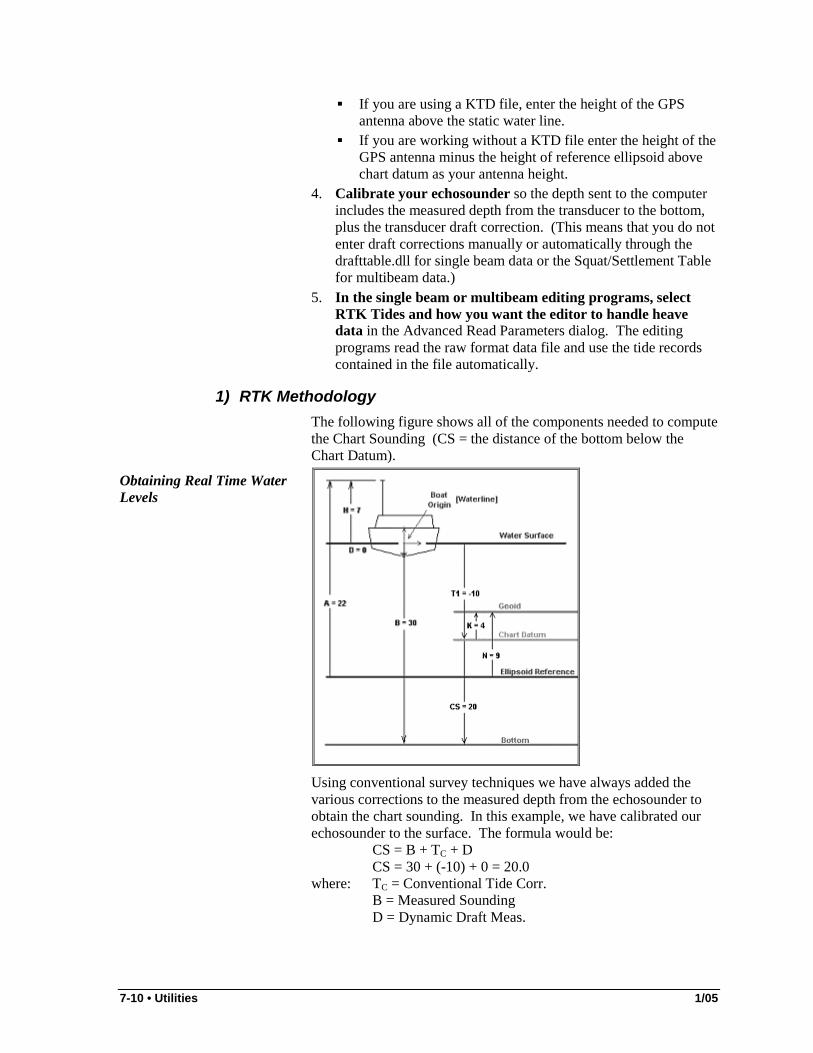
1) RTK Methodology The following figure shows all of the components needed to compute the Chart Sounding (CS = the distance of the bottom below the Chart Datum).
Obtaining Real Time Water Levels
Using conventional survey techniques we have always added the various corrections to the measured depth from the echosounder to obtain the chart sounding. In this example, we have calibrated our echosounder to the surface. The formula would be: CS = B + TC + D
CS = 30 + (-10) + 0 = 20.0 where: TC = Conventional Tide Corr. B = Measured Sounding D = Dynamic Draft Meas.

1/05 Utilities • 7-11
The basics behind the computation of RTK Tide is that we can use the z-value of our GPS antenna to determine the tide correction in real time.
Assuming the vessel is not pitching and rolling (which adds another level of difficulty), we can compute the RTK Tide Correction (TR) as follows: TR = -K + N – A + H – D
TR = -4 + 9 – 22 + 7 – 0 = - 10 where: K = Height of the Geoid Above the Chart Datum N = Height of the Geoid Above the Ellipsoid
Reference A = Height of the RTK Antenna Above the
Ellipsoid Reference H = Height of the RTK Antenna Above the Boat
Origin Point D = Dynamic Draft Measurement
K comes from a KTD (Kinematic Tidal Datum) file created by the user. • If you are using a geoid model (available in version 2.12 or
later) enter the height of the geoid above the chart datum (K).
Note: This means that the first time you use a geoid model, you need to create a new KTD file. • If you are not using a geoid model, enter the height of the
reference ellipsoid above the chart datum (K-N). (This method is the same as was used in versions earlier than 2.12.)
N is the height of the Geoid above the Ellipsoid (as read from the Geoid99 model in real time) plus an orthometric correction specified in the Geodetic Parameters program. If you are not using the geoid model, N=0.
A is the height of the antenna above the reference ellipsoid. This is broadcast as a part of a GGA, GGK or other message from our RTK system.. Every time the GPS.dll or Kinematic.dll device driver receives a position update, it computes the new position, along with a new RTK Tide value.
H is the static height of the RTK Antenna above the water line. In order to maximize accuracy, this measurement should be taken at the same time you calibrate your echosounder to the surface. In theory, this should be measured to the same point (boat origin = static waterline) that you are using to calibrate your echosounder. In actual practice, it’s not practical to measure the antenna height out in the middle of the channel when you are doing a bar check.
We suggest that you measure the antenna height when the vessel is at the dock and place a mark on the hull to denote the static waterline. Then make an adjustment to the antenna height when you calibrate the echosounder by noting the change in height of the waterline relative to the mark.

7-12 • Utilities 1/05
D (Dynamic Draft) represents the vertical movement of the transducer in the water column. If you are using RTK tides with HYPACK® (which presumably you are since you're reading this) you do not need to enter any draft corrections.
The device driver subtracts the dynamic draft correction to compute the "true" tide correction. Without a draft correction, the driver will still calculate a correct chart sounding, but the RTK Tide value will be different from the conventional tide value.
For example: In the previous figure, draft=0 and the RTK tide value is calculated to be –10.0 and the CS=20.
Now add a draft value of D=1, but do not provide a draft correction.
RTK setup with draft
The calculations then become:
TR = -4 + 9 – 22 + 7 – 1 = - 9.0 CS = 29 + (-9) + 0 = 20.0
If your vessel is prone to squat and settlement or sits differently due to fuel loading, we suggest that you let your RTK system calculate the tides for the best accuracy.
2) Using KTD Files A KTD file is used in cases where the separation between the two surfaces actually changes, depending on your location. SURVEY automatically loads a KTD enabled in your Project Files list.
You do not need to make a KTD file if: • the separation between your reference ellipsoid and chart datum
is a constant. • you are surveying in a small area and only want to use a single
separation value.
The values in the KTD file differ depending on whether you are using a geoid model.

1/05 Utilities • 7-13
If you are using a geoid model, the KTD file contains the height of the geoid above the chart datum.
Note: This means that the first time you survey an area using a geoid model, you must create a new KTD file.
If you are not using a geoid model, the KTD file contains the height of the reference ellipsoid above the chart datum (K – N). This is the same value as you would have used in HYPACK® versions earlier than 2.12.
3) Determining the Values for the KTD File Before you head out on the water to start your survey, you need to create your KTD File.
If you are not using a geoid, determine the height of the chart datum above the WGS-84 reference ellipsoid. (This is the same process used in HYPACK® versions before 2.12.)
If you are using a geoid, determine the height of the geoid above the chart datum (K).
If your survey is conducted in a small area, you may need only a single point. If your survey is conducted over a large area where the separation between the ellipsoid and chart datum changes, you will need several points to “model” the difference.
The following steps should be taken at each location to determine the KTD values.
Determining your KTD value
1. Set up your GPS adjacent to your tide staff. The staff should be referenced to the local chart datum.
2. Write down the water level from the tide staff (T). 3. Measure the distance from your GPS antenna to the water
level surface (H). 4. Once your GPS is stable and in RTK mode, write down the
height of the GPS antenna above the reference ellipsoid (A). This is normally contained in the GGA and GGK messages. It might also be available on the front data display of some GPS. You should take care to note whether your GPS provides this

7-14 • Utilities 1/05
value in feet or meters. If you are measuring depths in feet, you will need to convert the ellipsoid height of your antenna to feet. (1 meter = 3.280833333 feet).
5. If you are using a geoid model, record a reading from your geoid model (N). This is the height of the geoid above the Reference Ellipsoid.
6. Calculate the Value for the KTD file.
If you are using a Geoid Model K = – T – A + H – D + N = - (-10) – 22 + 7 – 0 + 9 = 10 – 15 + 9 = 4
If you are not using a Geoid Model
K - N = – T – A + H – D = - (-10) – 22 + 7 – 0 = 10 – 22 +7 = -5
4) Creating a KTD file in the KTD Editor The values in the KTD file differ depending on whether you are using a geoid model.
If you are using a geoid model, the KTD file contains the height of the geoid above the chart datum.
If you are not using a geoid model, the KTD file contains the height of the ellipsoid above chart datum (K – N). 1. Plot your survey area on a piece of paper. 2. Plot the location of your tide stations, where you have
determined the separation values. Write the separation values next to each gauge.
3. Draw a rectangular grid around your survey area. This is the border of your KTD file. Make a note of the lower left X-Y and upper right X-Y coordinates. They will be needed when you create the KTD file.
4. Determine how many "nodes" you want in each direction. The limit is 100 in each direction. See the following sample diagram.
Separations: Ellipsoid above Chart Datum

1/05 Utilities • 7-15
In this case, there are 3 nodes in the X-direction and 5-nodes in the Y-direction. 5. Contour the separation data, as shown in the diagram. 6. Determine a separation value at each node, based on the
contour information. 7. Start the KTD TIDE EDITOR by selecting PREPARATION-
EDITORS-KTD TIDE EDITOR. 8. Enter the maximum and minimum values for your X and Y
coordinates. These were obtained in step 3. 9. Enter the number of nodes (or divisions) in each direction.
The spreadsheet below will change to reflect the number you have entered.
KTD Editor
10. Enter the separation value for each node in the appropriate
grid. 11. Save your file by clicking FILE-SAVE and save the file to a
KTD file. KTD files can be saved anywhere, but we normally put them in the \MAX\PROJECT\(PROJECT NAME) directory.
5) Operating without a KTD File A KTD file is only necessary if you are in an area where the separation between the reference ellipsoid and chart datum is not a constant. If the separation is a constant, or if your survey area is so small, you don't need more than a single value, you can operate without a KTD file. In this case, you would also work without a geoid model.
You can "fool" the system by entering the combined value of your antenna height minus the height of the reference ellipsoid above chart datum as the height in the OFFSETS window in HARDWARE for the GPS.dll or Kinematic.dll.
7-16 • Utilities 1/05
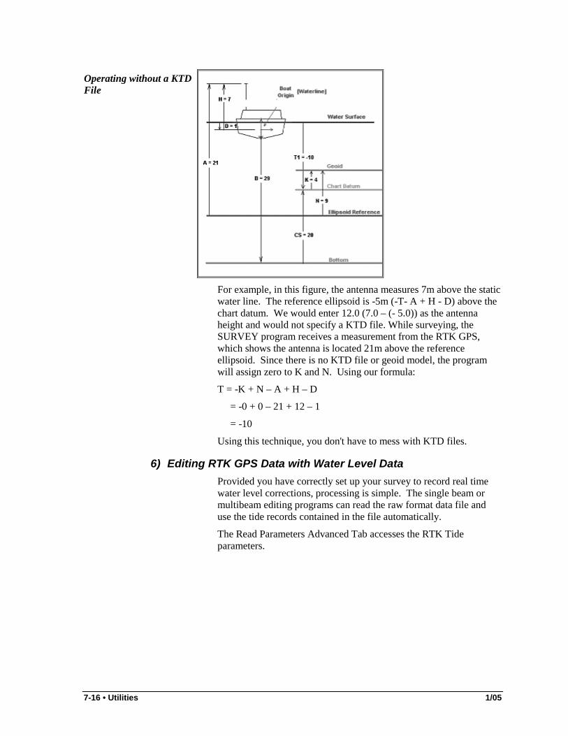
Operating without a KTD File
For example, in this figure, the antenna measures 7m above the static water line. The reference ellipsoid is -5m (-T- A + H - D) above the chart datum. We would enter 12.0 (7.0 – (- 5.0)) as the antenna height and would not specify a KTD file. While surveying, the SURVEY program receives a measurement from the RTK GPS, which shows the antenna is located 21m above the reference ellipsoid. Since there is no KTD file or geoid model, the program will assign zero to K and N. Using our formula:
T = -K + N – A + H – D
= -0 + 0 – 21 + 12 – 1
= -10
Using this technique, you don't have to mess with KTD files.
6) Editing RTK GPS Data with Water Level Data Provided you have correctly set up your survey to record real time water level corrections, processing is simple. The single beam or multibeam editing programs can read the raw format data file and use the tide records contained in the file automatically.
The Read Parameters Advanced Tab accesses the RTK Tide parameters.

1/05 Utilities • 7-17
The Advanced Read Parameters Dialog
If you check RTK Tides, SINGLE BEAM MAX will then use the RTK tide records written in the raw data file for tide corrections. This will activate the two options on how the program combines RTK water level elevations with heave corrections.
Merge Tide Data with Heave uses the RTK elevations as vertical “anchors”. Between the GPS elevation updates, the program “fits” the heave data to predict the change in vessel movement.
Average Tide Data to Remove Heave averages the RTK elevations over a user-defined time period to obtain a “normalized heave plane”. In theory, this average vertical level should be the zero plane as defined by the heave-pitch-roll sensor. The program then applies the exact heave corrections to the data to obtain the exact vessel position at the time of the depth measurement.
A time period of 30 seconds seems to work quite well.
The Invert Tide Values option should be checked in the Selections Tab when you are working in elevation mode using RTK Tide corrections.
7) Editing RTK GPS Data with Conventional Tides You can process raw data files that have RTK water level corrections using conventional tides by simply reading a TID file while in SINGLE BEAM MAX. This enables you to process the data using RTK water levels or conventional tide corrections, then compare the results in the CROSS SECTIONS AND VOLUMES program (or in the editor profile screen by using the Overlay feature).
II. Boat Shape Editor The Boat Shape Editor is used to create a custom boat shape that matches your survey vessel. You can start from scratch or import a

7-18 • Utilities 1/05
DGW file of your vessel to convert it to the SHP format used in HYPACK® MAX
Boat Shape Editor
A. Creating a Boat Shape 1. Establish an origin point on your survey boat. This should
normally be the location of the echosounder transducer. 2. Open the BOAT SHAPE EDITOR by clicking
PREPARATION-EDITORS-BOAT SHAPE EDITOR. Click on FILE-NEW to indicate that you are creating a new boat shape or FILE-OPEN to load a boat shape that you want to modify.
3. Describe your boat shape. Click the Boat Points list and begin to enter the X-Y points that describe the exterior of your vessel. The XY units match your survey units and are relative to the origin point. As you move the cursor to the next line, the current boat shape will draw on the screen. The program will automatically close your boat shape back to the first point in the list.
4. Enter your anchor points. Click on the bottom grid box for anchor points. You can enter up to nine anchor locations for your boat.
5. Describe any drawing objects by entering the XY points that describe the outline. Radius measurements (greater than half the distance between points) create arcs between the points. This feature can be used to draw boat features for visual effect only. The programs do not take them into account for any calculations.

1/05 Utilities • 7-19
6. Check which items you want to see drawn in the BOAT SHAPE EDITOR. ▪ Show Devices shows a list of devices in the upper left corner
of the drawing area. ▪ Show Offsets draws devices in position on the boat shape
according to the listing in the Survey32.ini. ▪ Show Anchor Points draws an "X" at each anchor point. ▪ Show Drawing Objects draws the lines described in the
Drawing Objects spreadsheet. 7. Save your File. When you are finished, click on FILE-SAVE
and name your Boat Shape file. It will be saved to the project directory with the .SHP extension.
The tools in the Shortcut Menu include:
Mirror Horizontal and Mirror Vertical mirrors the boat about the horizontal or vertical axis. They are very useful if your boat origin is on the centerline of the boat. Otherwise do not use them.
Add as Anchor: Select the boat point where an anchor is attached and select this option to add it to the Anchor Points list.
Offset Origin Point displays a dialog to define the distance in each direction to move the origin. Enter the offsets and click [OK]. The origin in the boat shape will shift and the offsets in the points lists will adjust accordingly.
B. Importing your Boat Shape If you have a DGW file of your boat shape, you can import it to the BOAT SHAPE EDITOR. The DGW file must have 1. Select FILE-IMPORT SHAPE. 2. Select the DGW File of your vessel. The coordinates will be
loaded into the Boat Shape Editor. 3. Save your file by selecting FILE-SAVE and naming your file. It
will be saved with the SHP extension to your directory.
III. 3D Shape Editor The 3D SHAPE EDITOR is used to create custom, 3-dimensional shapes. These shapes are saved to 3OD files and exported to VES files that can then be imported to the 3D TERRAIN VIEWER (3DTV or Matrix 3DTV) in order to provide the most realistic display possible.

7-20 • Utilities 1/05
A 3D Vessel Shape displayed in the 3D Terrain Viewer
Initially, the 3D SHAPE EDITOR can be used to create near replicas of your vessel. You can then import them to the 3D TERRAIN VIEWER programs and navigate on the virtual water there as you steer your vessel during your survey or dredging. Dredges constructed using 3D SHAPE EDITOR's dredge templates will be fully animated showing your digging tool at work.
A. 3D Shape Editor Interface Launch the 3D SHAPE EDITOR by selecting PREPARATION-EDITORS-3D SHAPE EDITOR.
The 3D SHAPE EDITOR Window
The 3D SHAPE EDITOR has a series of toolbars at the top that are used to create and manipulate various 3-dimensional shapes, which

1/05 Utilities • 7-21
can be put together to model your custom shape. Hold your cursor over any icon to view the icon name.
The Object Browser shows a tree view listing of each object as it is created. Simple objects (an individual object as it is created from the menu bars) can be listed under the root of the tree view, or grouped together into subgroups which appear as nodes on the tree view. Grouped objects create Complex objects which can then be selected then be translated or rotated as a unit within the design while maintaining each component object's size, orientation and position relative to the others in the group.
The Object Properties lists various attributes of a selected object as it is drawn in the design windows. Through the Object Properties, you can view and modify the name, size (by scaling), orientation (by rotating), position (by translating)" instead of "size, position (rotation and translation, color, transparency and texture. The effects of any modifications will be updated and displayed in the drawings.
The 4-paned design window enables you to view and manipulate your design from all angles. Right click and select "Change View" to toggle the 2-dimensional design windows (top, front or right side views) to show the opposite face (bottom, back or left side views respectively). The default background color is black, but you can choose a white background by selecting VIEW-WHITE BACKGROUND. To guide your drawing, you can toggle a display of rulers and grid tics through the VIEW ORTHO TOOLS menu.
Move 3D Camera Tool
The upper right pane is a 3-dimensional perspective view of your design which may be viewed from any angle using the "Move 3D Camera" tool.
B. Adjusting the View in 3D Shape Editor The 3D SHAPE EDITOR provides several options to optimize your view of your custom shape in the design panes. You can change the: • Model itself by changing the model type, color and shading. • Camera Position (viewing distance and angle) • Lighting to optimize your view
1) Model Type in the 3D Shape Editor
The Model menu provides a few display options which are also accessible through the Model tool bar. ▪ Solid draws an opaque, custom shape in the colors chosen
for the component objects in their object properties. ▪ Wire Frame draws your custom shape as a white
transparent line drawing. The selected wire-frame objects are displayed in color.

7-22 • Utilities 1/05
Wire Frame Model
2) Shading in the 3D Shape Editor ▪ Sharp Shading uses the same shade intensity on the whole
face, It shows the edges where faces are joined. ▪ Smooth Shading varies intensity of shade across the face in
a more realistic manner. It smoothes rounded shapes.
Solid Model
Sharp Shading
Solid Model
Smooth Shading
3) Object Color in the 3D Shape Editor The Default Color will be used when each new object is created.
You can change the object color after it is created by changing its Color property as described in "Setting Object Colors".
4) Lighting in the 3D Shape Editor Mining Lamp sets the position of the light source to match the camera position If you turn it off, the light will remain on the most recently illuminated side of the shape, regardless of its orientation in the design panes.
1/05 Utilities • 7-23
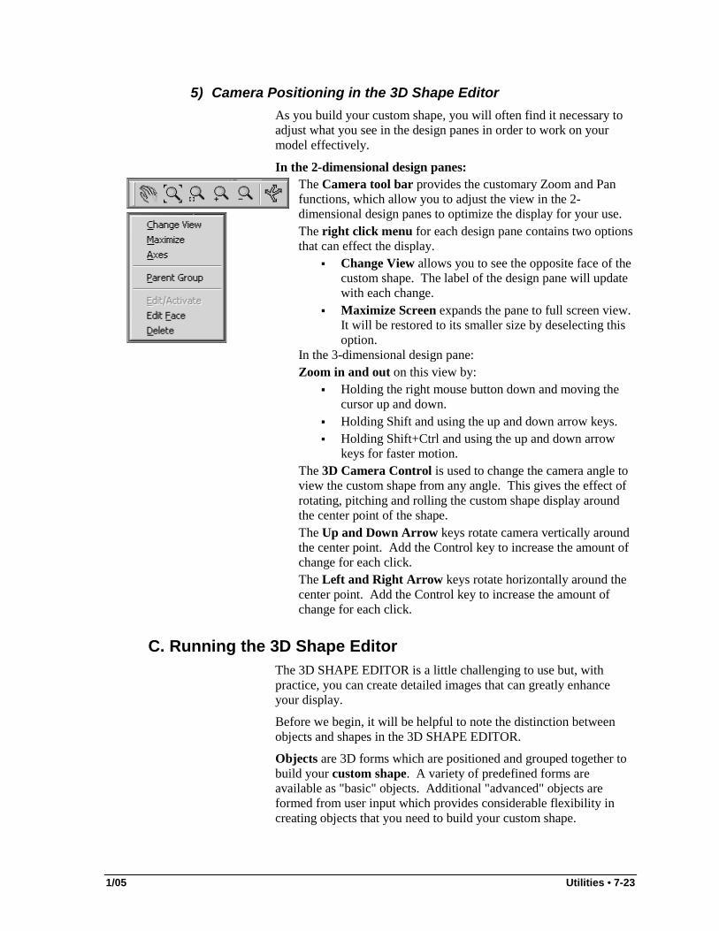
5) Camera Positioning in the 3D Shape Editor As you build your custom shape, you will often find it necessary to adjust what you see in the design panes in order to work on your model effectively.
In the 2-dimensional design panes:
The Camera tool bar provides the customary Zoom and Pan functions, which allow you to adjust the view in the 2-dimensional design panes to optimize the display for your use. The right click menu for each design pane contains two options that can effect the display.
▪ Change View allows you to see the opposite face of the custom shape. The label of the design pane will update with each change.
▪ Maximize Screen expands the pane to full screen view. It will be restored to its smaller size by deselecting this option.
In the 3-dimensional design pane: Zoom in and out on this view by:
▪ Holding the right mouse button down and moving the cursor up and down.
▪ Holding Shift and using the up and down arrow keys. ▪ Holding Shift+Ctrl and using the up and down arrow
keys for faster motion. The 3D Camera Control is used to change the camera angle to view the custom shape from any angle. This gives the effect of rotating, pitching and rolling the custom shape display around the center point of the shape. The Up and Down Arrow keys rotate camera vertically around the center point. Add the Control key to increase the amount of change for each click. The Left and Right Arrow keys rotate horizontally around the center point. Add the Control key to increase the amount of change for each click.
C. Running the 3D Shape Editor The 3D SHAPE EDITOR is a little challenging to use but, with practice, you can create detailed images that can greatly enhance your display.
Before we begin, it will be helpful to note the distinction between objects and shapes in the 3D SHAPE EDITOR.
Objects are 3D forms which are positioned and grouped together to build your custom shape. A variety of predefined forms are available as "basic" objects. Additional "advanced" objects are formed from user input which provides considerable flexibility in creating objects that you need to build your custom shape.

7-24 • Utilities 1/05
A very over-simplified sequence to create a custom shape might be: 1. Open a 3OD file. This file contains all of the information about
your custom shape. You can either create a new one or open an existing file to modify.
2. Select an object from one of the tool bars and place it in the design window.
3. Set the object properties. Properties include: ▪ Scale ▪ Position ▪ Rotation
▪ Color ▪ Texture ▪ Transparency
4. Repeat using various objects as "building blocks" to "build" a vessel that matches yours and grouping the objects where appropriate.
5. Save your custom shape by selecting FILE-SAVE (or FILE-SAVE AS) and naming your file. It will be saved, by default, to your Hypack\Shapes directory with a 3OD extension.
6. Export your shape to VES format for use in the 3D TERRAIN VIEWER.
Note: If you make a change that turns out not to be what you had in mind, click the "Undo" button to reverse the action. The "Redo" button reverses the "Undo".
Each step will be detailed in the following sections.
D. Opening Custom Shape Files in the 3D Shape Editor To create a new shape, select FILE-NEW. A dialog will appear providing a choice of shape templates. A template is a predefined 3D shape file with certain unalterable features including object groups, the number, orientation and names of axes that create joints on mobile dredge parts, and the number and names of wire-attach points.
If you are creating a dredge with moving parts, you must modify the template most closely resembling your vessel. Excavator, cutter suction and hopper dredges have additional selections to further describe them.
Crane
Cranes have no additional settings.

1/05 Utilities • 7-25
Cutter Suction Dredge
Excavator
Hopper Dredge
If you are creating a shape other than a dredge, you should choose the "Free" option and build it yourself.
If you want to modify an existing custom shape, you can re-open a 3OD file in the 3D SHAPE EDITOR at any time.
FILE-OPEN and FILE-IMPORT 3OD load an existing 3OD file to the 3D SHAPE EDITOR. They default to the location to which you last exported 3OD file or from which you last imported a 3OD file • FILE-OPEN opens a previously saved 3OD file. • FILE-IMPORT 3OD imports the design in a user-selected 3OD
file into another. a. Open the 3OD file into which you want to add the other. b. Select FILE-IMPORT 3OD and choose the file to add in. A
copy of the imported file will be added to the active group of your current 3OD file. The imported file will not change.

7-26 • Utilities 1/05
E. Animating Dredge Template Files in the 3D Shape Editor Dredges and digging tools created from the dredge templates can be animated in the 3D SHAPE EDITOR to preview the type of motion you might expect during DREDGEPACK®.
Use the Animation tool bar to start and stop the preprogrammed motion. The dredge shape will repeat the animation loop, which depicts typical motion for the type of dredge you have chosen, until you click the stop button. While it is in motion, you can zoom, pan and rotate the model to inspect it from any angle you desire.
Note: Animation is not available when VIEW–WHOLE MODEL is selected.
F. Creating Basic Objects in the 3D Shape Editor The Basic Objects tool bar provides a choice of basic 3-dimensional shapes that can be used as components of your custom shape.
Basic Objects Toolbar
Just click the icon corresponding to the shape you need, then click in any of the 2-dimensional design panes to place the object in its approximate position. You will set exact positioning, as well as other properties, in the properties toolbar. (See "Setting Object Properties".)
G. Creating Advanced Objects in the 3D Shape Editor The Advanced Objects toolbar enables you to create more complex shapes that might be useful in creating your custom shape. The first four will each access the Object Modeling Window where you draw the footprint of the desired shape and set any applicable additional settings. When that is completed, the finished shape is created according to the icon selected and "floats" at the end of your cursor ready to be positioned in any of the 2-dimensional views.
Advanced Objects Toolbar
The Prism top and bottom faces match the user-defined footprint. Side faces are drawn by connecting corresponding points on the base and the top.
The Pyramid creates an edge of the pyramid between each point that defines the footprint and a point that is above the base. When you select a pyramid shape, the Object Modeling window includes sloped option which allows you to offset the apex.
The Truncated Pyramid forms a face parallel to the base that is a smaller scale version of the footprint. The side faces are drawn by connecting corresponding points on the base and the top. When you

1/05 Utilities • 7-27
select a truncated pyramid shape, the Object Modeling window includes ratio and sloped options.
The Hull uses the user-defined footprint as the base. A scale version of the footprint forms a parallel top face. Side faces are drawn by connecting corresponding points on the base and the top. The outer edges, however, are bowed rather than straight in an attempt to approximate the shape of a boat hull. When you select a hull shape, the Object Modeling window includes the sloped, ratio and slices options with which you can control the object shape.
The Revolution object uses a user-defined object profile, which is then repeated around the Y axis to complete the object form. When this object is selected, the Object Modeling window will only allow you to draw a right profile.
Additional Settings may include: • The "Sloped" checkbox creates a prism in which the upper face
is offset from the lower face, which results in a prism with sloped sides. The offset is determined by the distance off center that you draw the footprint on the drawing board.
• Ratio defines the proportion of the upper face compared to the lower face. The value must be in the range from 0.01 to 10 inclusive.
Ratio Value Result < 1 a top face smaller than the bottom. The
hull sides are concave. = 1 a prism > 1 a top face larger than the bottom. The
hull sides are convex. • Slices determines the number of segments in the line that
connects the upper to lower face. The value must be in the following ranges:
Object Allowable Values
Result
Hull 1-20 A value of 1 results in straight lines joining each corresponding point on the upper and lower faces (a truncated pyramid) and 20 creates a smoothly curved surface. This is most clearly visible in the top or bottom view.
Revolution Object
3-30 This value sets the number of sides in a horizontal cross section of the object. 30 makes a smoothly round cross section.
Note: Increase the number of slices – better presentation quality will be achieved, but slower refresh rate may result in 3DTV.
1) Object Modeling Window When you select any of the advanced object icons, the Object Modeling Window will automatically appear.

7-28 • Utilities 1/05
Object Modeling Window
The white area is your drawing board. In its simplest presentation, it is only bisected, both vertically and horizontally by a plain line. You can add further drawing guides by selecting various icons from the tool bar as follows:
Icon Name Icon Added Drawing Guide
Axis Marks Tics at each quarter distance along each axis.
Grid Dots marking a grid at intervals of 0.05 units.
Snap to Grid
Assists in keeping sides straight and aligned with the drawing board grid.
Vertical Ruler
Draws a straight vertical line from first point (an end point) defined by cursor to the levels of each subsequent position.
Horizontal Ruler
Draws a straight horizontal line from first point (an end point) defined by cursor to the levels of each subsequent position.
Vertically Symmetric
Automatically mirrors a user-defined shape drawn above the horizontal axis in the area below.

1/05 Utilities • 7-29
Icon Name Icon Added Drawing Guide
Horizontally Symmetric
Automatically mirrors a user-defined shape drawn left the vertical axis in the area on the right.
Note: The length of each axis is one unit in each direction from the center 0,0 point. You can further adjust the scale of your component pieces in the object properties. The scale of your custom shape can also be adjusted in the 3D TERRAIN VIEWER in the Vessel Settings dialog.
A small preview of your object is shown below the drawing board. If it doesn't look right to you, go back to the drawing board!
2) Drawing Advanced Object Faces in the Object Modeling Window
Add Point Icon When the Object Modeling Window appears, the cursor defaults to the drawing pencil cursor (the Add Point icon is selected). .
1. Select the drawing board features that are helpful to you. 2. Use the cursor to draw the footprint of your custom shape.
The OBJECT MODELING WINDOW will automatically close the polygon when you: ▪ deselect the Add Point icon ▪ hit the Enter key ▪ click on the first point.
3. Set slope, ratio and slices options where applicable to the chosen object.
4. Preview the described shape in the lower area of the window. If the shape is not as you had planned, you can "go back to the drawing board" (literally) and either modify what you have created or erase it and start over.
5. Modify your shape, if necessary, using the editing tools. (See "Editing Advanced Objects".)
6. When you are satisfied with your shape, click [OK]. The dialog will close and your shape will be ready at the end of your cursor to be placed in your custom shape design.
7. Place the object in its approximate position by clicking in any of the 2-dimensional design panes. You will set exact positioning in the properties toolbar. (See "Positioning Objects into you Custom Shape".)
3) Editing Advanced Objects Once you have a closed polygon on your drawing board. There are several ways that you can modify the size and shape.
Select Icon To move a point, click the Select icon. Use the cursor to drag existing points in your polygon to new positions.

7-30 • Utilities 1/05
Insert Point Icon
To insert a point, click the Insert Point icon. (The cursor will return to the pencil.) Use the cursor to click where, on the polygon edge, you need an additional defining point. If you click elsewhere in the drawing board, the Object Modeling window will include the added point to the nearest polygon segment and adjust the shape accordingly.
Delete Point Icon
To delete a point, click the Delete Point icon (the cursor will change to an eraser) then click the point that you want to remove from your footprint shape.
The OBJECT MODELING WINDOW also includes some additional tools that may help you achieve the results you need. The Copy and Paste icons may be helpful particularly if you are working with complex shapes.
Copy Icon
Paste Icon
The Copy and Paste functions work together. The Copy icon stores the polygon as it appears in the drawing board to a temporary memory. You can restore the drawing board with the most recently copied shape using the Paste icon. Using this pair of features, you can modify a footprint incrementally, saving each change or set of changes as you progress by clicking the Copy icon. At any time during the modification process, you can return to the most recently copied shape by clicking the Paste icon. The copied shape is stored even after leaving the Object Modeling window. This enables you to create multiple advanced objects with identical footprints by copying the first footprint, then pasting it into the drawing board for the subsequent advanced objects.
Delete Polygon Icon
To erase the polygon, from the drawing board, click the Delete Polygon icon.
Note: You can also use the Object Modeling window to modify advanced shapes after they are placed in your design window. Right click on the object in the Object Browser or in one of the design panes and select "Edit/Activate Face" (or double click the object)
H. Creating Vessel Origin and Attachment Points When you create a custom shape to represent your vessel, the vessel origin and, if it's a dredge, the attachment points for dredge arms and spuds are required for HYPACK® to accurately position the vessel and its moving parts.
Note: You should only specify the attachment points, spuds and dredge arms will be drawn in 3DTV, if SURVEY sends information through Shared Memory.
The vessel origin, as you probably know by now, is the key to accurately positioning everything in SURVEY! Position the origin in your 3D vessel in the same position as in your hardware setup.

1/05 Utilities • 7-31
On a dredge, the attachment points for dredge arms and spuds should also be included. (You can attach up to three items.) When your vessel is imported into the 3D TERRAIN VIEWER: • Dredge arms are represented by a single cylinder between the
attachment point and the digging tool. • Spuds are represented by a vertical cylinder:
▪ At the attachment point, or ▪ connected with attachment point by horizontal cylinder if the
spud is placed on motorized carrier.
The cylinders' diameter and color, as well as cylinder length for vertical bar, should be set in 3DTV.
I. Removing Objects from the Custom Shape Any object can be easily removed from the custom shape design by any of the following methods: • Select the object and hit the Delete key. • Right click on the object and select Delete from the pop-up
menu.
J. Setting Object Properties in the 3D Shape Editor Once you have set an object into your design panes. You will probably need to adjust its size, orientation and position in the design, and possibly its color and transparency, or texture as well. These are the object properties.
You can modify the properties of a selected object or objects with tools from the Transformations or Alignment and Distributions tool bars or by changing the values in the Object Properties.
Transformations Toolbar Alignment and Distribution Toolbar
Object Properties

7-32 • Utilities 1/05
When you want to change any of the object properties, the object itself must first be selected. When an object is selected, its properties are displayed in the Properties dialog and the object is highlighted in the Object Browser and design panes.
To select an object:
Select Tool Icon Use the Select Tool by clicking the icon then the object in one of the 2-dimensional design pane windows. Use the cursor by clicking on the object in the Objects Browser.
Alignment and distribution, as well as grouping operations, require selection of multiple objects or groups.
To select multiple objects or groups: Hold your Ctrl key and click on each object you want to select. (You can click in either the Object Manager or a 2D design window.) The name of each selected object will be highlighted in the Object Manager.
When a multiple selection is complete, the right click menu will enable only operations that can be applied to all of the selected objects, such as Group, Ungroup, Move Up and Delete.
1) Positioning Objects into your Custom Shape You can fine-tune the XYZ positioning and the rotation of an object by adjusting the translation and rotation properties listed in the Object Properties dialog.
(a) Translating Objects Translation is simply moving the object to a new position within your design while maintaining its original orientation.
The transformations tool bar has three translation tools. Select the appropriate tool for your purpose then use it to drag the object into position in your 2D design panes. The translation values in the Properties dialog will update accordingly. Which values are affected depends on which tool you use and which pane you use it in.
The Horizontal Translation tool moves the selected object in a straight horizontal line. There will be no vertical change even if your cursor position moves vertically.
▪ Used in the Back /Front or Top/Bottom pane, this tool affect the TransX value.
▪ Used in the Side pane, it affects the TransY value.
The Vertical Translation tool moves the selected object in a straight vertical line. There will be no horizontal change even if your cursor position moves horizontally.
▪ Used in the Back /Front or Side pane, it affects the TransZ value.
▪ Used in the Top/Bottom pane, it affects the TransY value.
The Translation Tool moves the object in any direction with your cursor.

1/05 Utilities • 7-33
You can also modify the translation values directly in the Properties dialog. TransX, TransY and TransZ move the object parallel to the X, Y and Z axes respectively.
Translation values of 0,0,0 places the object at the center of the design area.
(b) Rotating Objects Rotation turns the object around one of the axes. The axis around which it turns depends on the pane in which you use the tool.
The Transformations tool bar contains a Rotation tool with which you can rotate the objects in the 2D design panes. The Rotation values in the Properties dialog will update accordingly. • In the Top/Bottom pane, the object rotates around the Z axis. • In the Right/Left pane, the object rotates around the X axis. • In the Back/Front pane, the object rotates around the Y axis.
You can also modify the rotation values directly in the Properties dialog. RotX, RotY and RotZ rotate the object around the X, Y and Z axes, respectively.
Note: These angle values are given in the XYZ order convention, meaning that rotations are performed around axis strictly in that order: first around X-axes, then around Y-axes, and finally around Z-axes. When you rotate an object through 2D panes, those three angles well be recalculated to reflect the given rotation applying the order of rotations convention.
(c) Aligning Objects Alignment is placing two or more objects or groups in a line relative to each other. The 3D SHAPE EDITOR can align objects horizontally or vertically in the top design window. • Vertical alignment is based on their top, center or bottom
points. • Horizontal alignment is based on their left, center or right
points.
The tools in the alignment and distribution toolbar only become active if you have selected multiple objects or groups, or a combination of both.
Note: Selecting one group is not the same as selecting its component objects. 8. Select multiple objects or groups: Hold your Ctrl key and click
on each object you want to select. (You can click either in the Object Manager or a 2D design window.) The name of each selected object will be highlighted in the Object Manager.

7-34 • Utilities 1/05
9. Once you have selected the items you want to align, just click the icon appropriate for the type of alignment you want to accomplish.
The figures below show the effects of each operation. The three objects begin in the original arrangement and are all selected. They are then aligned using one of the six alignment icons.
Original Arrangement
Horizontal Alignment Icons
Left
Center
Right
Vertical Alignment
Top
Center
Bottom
(d) Distributing Objects Distributing evenly spaces objects or groups based on their center points. In the following diagrams, we see that the original arrangement from our previous example has three objects that are both horizontally and vertically distributed.
Object Distribution
Horizontal Distribution
Vertical Distribution
2) Setting Object Physical Attributes In addition to positioning each object in your design, you can also define what they look like. Color, Transparency and Texture can also be defined in the Object Properties.

1/05 Utilities • 7-35
Color, Transparency and Texture properties can also be applied to individual faces of an object by editing the face. (See "Editing Object Faces".)
(a) Setting Object Colors As you build your custom shape you can color the component parts. This can be helpful in distinguishing one object from another within your custom shape. It can also enhance the appearance of your custom shape by making it a bit more realistic.
The default color will be used when each new object is created. If you want several objects of the same color, set the default and create them. The same color will appear for each object in the Properties dialog.
To set the default color, click the default color icon on the Model tool bar and select the desired color from the color dialog.
To change the Color Property of any object click the color in the Properties dialog and choose the new color from the color dialog that appears.
(b) Setting Object Transparency Transparency makes the entire object transparent. If this property is set to "Yes", all of the object faces appear transparent. A transparent object will retain the designated color, but you will be able to see objects that are inside or behind them. The following figures demonstrate the difference. The transparent sphere allows you to see the parts of the cubes and cone that are hidden when it is solid.
All Solid Objects (left)
Transparent Sphere (right)
The Transparency property may be applied to an object face. In the following example, one face of the cone is transparent, which allows you to see inside to the red base. (See "Editing Object Faces".)
Transparent Face

7-36 • Utilities 1/05
(c) Setting Object Textures 3D SHAPE EDITOR has a selection of graphics that can be applied to your object to provide more realistic texture or a graphic to your shape.
Note: Textures override color and transparency properties.
To add a texture or graphic to your shape: 1. Click in the Texture property. The Texture dialog will appear.
Texture Dialog
2. Select your texture or graphic from:
▪ From the 3D Shape Editor library. ▪ From your own files by clicking [More] and selecting a
BMP file. Your BMP must measure 2n pixels where n equals any value 1 to 11 (maximum 2048px).
3. Set your display options. ▪ Magnification and Minification Filters ▪ Tiling causes the graphic to repeat edge-to-edge. The X and
Y values determine how many repetitions per length unit, horizontally and vertically there will be. If your object is the default 2 units in size, the number of repetitions will be double the value that you enter in the dialog.
4. Click [OK] to return to 3D SHAPE EDITOR.
Whale Graphic—
No Tiling (left)
Tiled (right)

1/05 Utilities • 7-37
(d) Setting Object Visibility The Visibility property lets you choose, on an object-by-object basis, which objects in your custom shape are drawn to the 3D SHAPE EDITOR design panels. (Any object with a Visible property of "Yes" will be drawn.)
Additional tools affect multiple objects and groups.
VIEW-ATTACHMENT POINTS toggles the Visibility property of all joints and the origin.
A "Make All Objects Visible" icon on the tool bar resets all object Visible properties to "Yes" so that all objects can be displayed.
VIEW-WHOLE MODEL overrides the Visibility properties and displays all objects regardless of which object or group is selected. If this option is not selected, only the objects of an active group will be drawn.
(e) Scaling Objects Scaling is changing the size of the object. The Scaling tools in the 3D Shape Editor can be used to scale only individual objects. The shape can also be further scaled when it is displayed in the 3D Terrain Viewer.
The Transformations tool bar includes several tools you can use in the 2D design panes to scale your object to suit your needs. The Scale values in the Properties dialog will update accordingly. Which scale values your adjustments affect depends on the pane in which you use the tool.
Horizontal Scale Tool expands and contracts the object horizontally in the pane.
▪ In the Top and Front panes, it affects the ScaleX value. ▪ In the Side Pane, it affects the ScaleY value.
The Vertical Scale Tool expands and contracts the object vertically in the pane.
▪ In the Top and Side panes, it affects the ScaleY value. ▪ In the Front Pane, it affects the ScaleZ value.
The Increase and Decrease Scale Tools increase and decrease the scale in all three directions. The Fast tools (double arrows) change the scale by 10%. The slower tools change the scale by 1%.
You can also modify the scale values directly in the Properties dialog. ScaleX, ScaleY and ScaleZ affect the scale of the object along the X, Y and Z axes respectively.

7-38 • Utilities 1/05
3) Editing Object Faces When a solid (non-wire framed) object is created, all sides are opaque and of the default color. Objects in the world are rarely so. Some sides may be of different colors or textures, or have windows and doors. All of these characteristics can be included in your custom shapes by editing individual object faces. 1. Access the Face Editing Window by right clicking on the face
that you want to edit and selecting "Edit Face" from the pop-up menu. The Face Editing dialog appears with an outline of the selected face on the drawing board.
Note: This dialog draws the selected face in the largest scale possible without exceeding the size of the drawing board. If you drew this face originally, it will probably be a different scale here.
Face Editing Dialog
2. Edit the face. Color, texture and transparency can be specified
for the selected face in much the same way as those properties can be applied for an object. The same color and texture dialogs that are used for the object are accessed to modify the face ▪ To change the face color, click [Color] and select the color
from the dialog that appears. ▪ To add a texture or graphic to a face click [Texture] and
select the texture options for the selected face as you would for an object. (See "Setting Object Textures".)
▪ To make the face transparent, click the "Transparency" check box.
▪ To create a design or window on the face. i. Draw the window shape within the face outline using
the drawing tools. The Window properties will become enabled.
ii. Set Color, Texture or Transparency properties for the window shape. These properties will be applied to

1/05 Utilities • 7-39
the window independently of the face and object properties.
▪ To include more than one window on a side, you must use an advanced object and define one side with more than one face. Here's an example of how it works.
Suppose your vessel's cabin has both a window and a door on one side.
i. Create the cabin object. You must use an advanced object. In this case, we'll use a prism.
ii. Draw a rectangle, sized to match your cabin, and including a point somewhere between where the window and door will be placed. In the following figure, the bottom edge is divided into two faces by drawing it as a 2-segmented line.
Creating Multiple Faces on One Side of an Advanced Object
iii. Place the object in the design panes. iv. Right click to one side of the divided face in one of
the 2-dimensional design panes and select FACE EDIT. The Face Edit dialog will appear. Notice the relative dimensions of the face it represents. If it isn't the shape you would expect based on what you've drawn, you may have the wrong face.
v. Draw the window, set the window color and transparency and click [OK].
vi. Repeat steps 4 and 5 at the opposite end of the side (the other face) for the door.
7-40 • Utilities 1/05
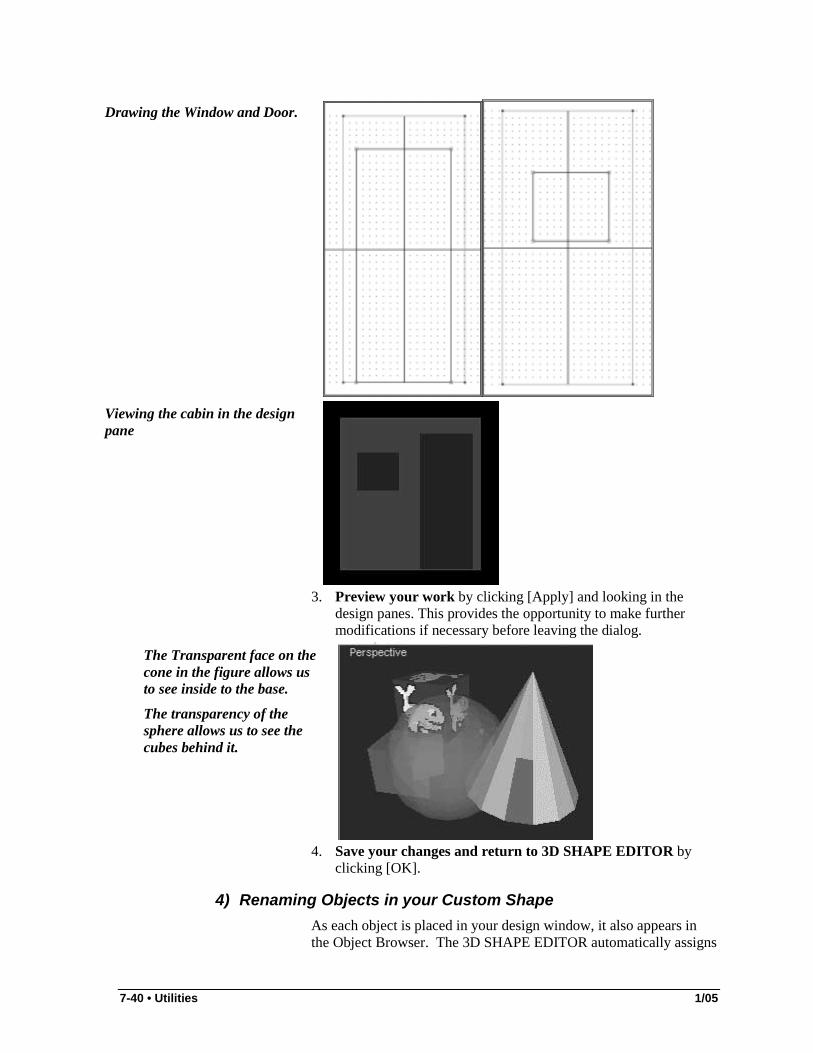
Drawing the Window and Door.
Viewing the cabin in the design pane
3. Preview your work by clicking [Apply] and looking in the
design panes. This provides the opportunity to make further modifications if necessary before leaving the dialog.
The Transparent face on the cone in the figure allows us to see inside to the base.
The transparency of the sphere allows us to see the cubes behind it.
4. Save your changes and return to 3D SHAPE EDITOR by
clicking [OK].
4) Renaming Objects in your Custom Shape As each object is placed in your design window, it also appears in the Object Browser. The 3D SHAPE EDITOR automatically assigns

1/05 Utilities • 7-41
a name according to the object type and the number of that type of object already in your design. If you prefer a different name, you can: • Enter a new name in the Object Properties dialog. • Right click the object name in the Object Browser, select
"Rename" and type in your preferred name.
K. Replicating Objects in your Custom Shape You can quickly and easily create multiple objects of the same size, shape and color using the "copy" and "paste" method. This option can be handy in creating items, such as railings or ladders, that have several identical pieces. 1. Create the first object as described in the previous sections. 2. Copy the object. There are two methods to do this with same
results: ▪ Click on the object in one of the design windows or in the
Object Browser, and select EDIT-COPY (Ctrl + C). ▪ Right click the object, in the Object Manager or in a 2D
design window, and select Copy from the pop-up menu. 3. Paste the object into your custom shape. There are two
methods to do this, each with different results. ▪ Select EDIT-PASTE (or Ctrl + V) and a duplicate object will
appear at the origin of the active group. ▪ Right click at the location in your custom shape where you
want the duplicate object to be positioned and select Paste from the pop-up menu. The duplicate object will be centered on your cursor position.
L. Grouping Objects in your Custom Shape Grouping allows you to join two or more objects in your design into a subgroup. Groups can be created either before or after their member objects have been created. You can then activate a group or subgroup for editing and work only with the member objects and subgroups.
Note: Activating a group or object is different than selecting a group or object. Active groups are indicated with bold text in the Object Browser and are available for editing.
To activate a group: • Double click on the object or group in the Object Browser. • Right click on the object or group in the Object Browser or in a
design pane and select Edit/Activate. • Right click on a selected sub-group and select Group Up.
When a group is activated, the activated group of objects will be shown in the design panes, while objects outside the group are hidden. You can:

7-42 • Utilities 1/05
• Add or delete objects in the group. • Modify the properties of individual objects within the active
group. • Translate or rotate subgroups of the active group as a unit
within the design while maintaining their size and position relative to each other
Note: Color, Texture and Transparency properties are disabled for grouped objects. They must be set for each individual object. • Ungroup the components of the group.
1) Grouping Existing Objects You can create several objects, and group them afterward into one or more groups. This allows you to build the custom shape, or a portion of it at a time, then organize the component objects into groups. These groupings will be subgroups of the folder in which they began. You can create multiple layers of groups and subgroups to suit your purposes.
If you are building a complex shape such as a dredge, we recommend that you build a few objects at time, then group them. This method is less confusing and allows you to move groups as you build, which can often be easier and more efficient
Group Selected Objects Icon
1. Build your custom shape without grouping your objects. Initially all component objects will be in Group_1. Subsequent objects will be in whichever group is selected when the object is created.
2. Select the objects to be included in a subgroup by holding the Control key and clicking on each object in the design window or Object Browser.
3. Click the "Group Selected Objects" Icon on the Advance Objects toolbar. The selected items will be grouped and the Object Browser will be updated accordingly.
Note: If you miss an object or two when you build the group, you can immediately use the "Undo" button to ungroup them, then try again. "Undo" reverses each action you perform in the window in the reverse order that you did them, so it is best that you check each group for completeness before you go on to your next step.
The following diagrams illustrate how objects can be grouped as you build your custom shape. Vessel origin is not visible in the figures on the right.

1/05 Utilities • 7-43
1) a prism forms the dredge
3) Add cubes and cylinders for the pump system and 2 attachment points for the spuds
2) Add a prism for the cabin and 2 cylinders to form the A-Frame
4) Several cylinders create each railing and the winch
2) Grouping Objects as you Build your Custom Shape If you prefer, you can create empty folders then create the objects that belong in them. This means you can either: • Create the entire hierarchy of groups, then add the shapes
appropriate to each afterward or • Create one new group at a time and fill each one as you build
your custom shape. 1. Right click on the group in the Object Browser where you
want to create a subgroup. A pop-up menu will appear. 2. Select "Add Empty Subgroup". A new Group will be created
under the original group. 3. Activate the group to which you are adding the new object.
(The group name will be bold.) 4. Create the object. The object will be added to the active group.
When you activate a sub-group of objects, all others in your design are hidden. This sometimes makes it difficult to position one group relative to another. In this case, activate the group in which the subgroup is a member and select the subgroup. The higher level group objects will be displayed, but you will still be moving the objects in the selected subgroup.
3) Naming your Groups As each Group is created, by default, it is named "Group_GroupNumber". You can rename any group by right clicking on the group name and selecting "Rename". The group name will become editable. Just type in the new name and hit the Enter key.
7-44 • Utilities 1/05
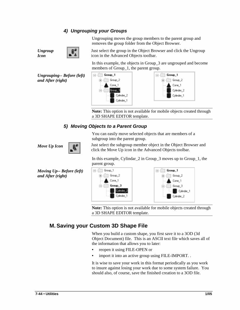
4) Ungrouping your Groups Ungrouping moves the group members to the parent group and removes the group folder from the Object Browser.
Ungroup Icon
Just select the group in the Object Browser and click the Ungroup icon in the Advanced Objects toolbar.
In this example, the objects in Group_3 are ungrouped and become members of Group_1, the parent group.
Ungrouping-- Before (left) and After (right)
Note: This option is not available for mobile objects created through a 3D SHAPE EDITOR template.
5) Moving Objects to a Parent Group You can easily move selected objects that are members of a subgroup into the parent group.
Move Up Icon
Just select the subgroup member object in the Object Browser and click the Move Up icon in the Advanced Objects toolbar.
In this example, Cylindar_2 in Group_3 moves up to Group_1, the parent group.
Moving Up-- Before (left) and After (right)
Note: This option is not available for mobile objects created through a 3D SHAPE EDITOR template.
M. Saving your Custom 3D Shape File When you build a custom shape, you first save it to a 3OD (3d Object Document) file. This is an ASCII text file which saves all of the information that allows you to later: • reopen it using FILE-OPEN or • import it into an active group using FILE-IMPORT. .
It is wise to save your work in this format periodically as you work to insure against losing your work due to some system failure. You should also, of course, save the finished creation to a 3OD file.

1/05 Utilities • 7-45
You can overwrite the same file each time, or use FILE-SAVE AS to save incremental records of your shape as it progresses.
To convert your custom shape to a format that can be imported to the 3D TERRAIN VIEWER, you must export the finished custom shape information to a VES file. When you build a custom
1) Saving 3OD Files You can save your 3OD files manually or automatically to the default Hypack\Shapes directory or to any other directory. The program will "remember" the last location to which you saved your 3OD file, or from which you opened your last 3OD file. This may save you some navigating through the file hierarchies every time you save your work outside of the HYPACK® default location.
To save your 3OD files manually, select FILE-SAVE, or FILE-SAVE AS and name your file.
To save your 3OD files manually, select FILE-SAVE and name your file.
To save your 3OD files automatically at user-defined intervals. 1. Select FILE-AUTOSAVE and the Auto Save dialog will
appear.
Auto Save Dialog
2. Check the Auto Save check box and enter a time interval (in
minutes) at which your design should be saved. 3. Click [OK].
Note: If this option is selected and you have not yet named your shape, a dialog will appear after the first time interval for you to provide a name.
2) Exporting your 3OD File to the Network FILE –EXPORT 3OD saves your 3OD file outside of the default Hypack\Shapes directory.
3) Converting your Custom Shapes to a VES File When your custom shape is complete, if you want to use it in the 3D Terrain Viewer, you must first export it to a VES file.
Select FILE-EXPORT VES…and name your file. It will be saved by default to the folder where you have most recently saved a VES file.

7-46 • Utilities 1/05
We suggest that you name your VES file with the same name as its corresponding 3OD file. If you do this, it will be easy to know which 3OD file you will need if any modifications are ever needed.
IV. Advanced Channel Design The Advanced Channel Design program is useful in designing complex channels for use as surfaces in volume computation in the TIN Model program. You can define any channel shape either by manually describing it or by importing data from Planned Line files or XYZ format files.
When the channel design is complete, it will be saved with a CHN extension to your project directory.
A. Running Advanced Channel Design 1. Open the program by selecting UTILITIES-ADVANCED
CHANNEL DESIGN. 2. If you wish to access an existing file, select FILE-OPEN and
select your Channel File. 3. Select WINDOW-NODES and enter (or edit) the node
information. 4. Select WINDOW-FACES and enter (or edit) the face
information. 5. Check your faces by selecting FACES-CHECK FACES in the
Faces dialog. The program will check each face for the following standards: ▪ All nodes are in the same plane ▪ Face is convex ▪ Face orientation (Nodes should be defined in counter
clockwise direction.) 6. Save your file by selecting FILE-SAVE or FILE-SAVE AS and
naming your file. The data will be saved with a CHN extension to the directory of your choice. Typically, it would be stored to your project directory.
B. Creating (or Editing) your Channel File in Advanced Channel Design
1) Entering Node Data in Advanced Channel Design Nodes are points where any of the faces of your channel surface have a corner. 1. Select WINDOW-NODES to define the nodes of your channel.
A four-column spreadsheet appears.
1/05 Utilities • 7-47
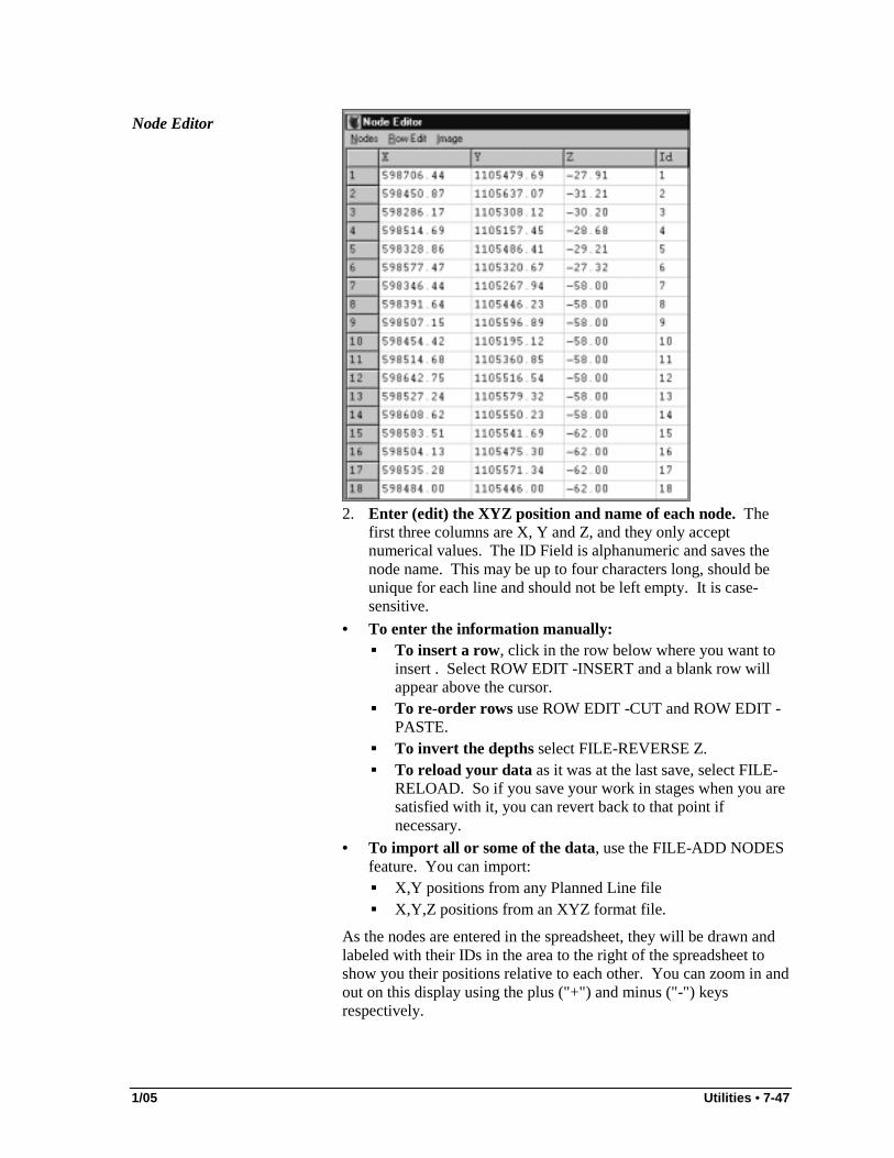
Node Editor
2. Enter (edit) the XYZ position and name of each node. The
first three columns are X, Y and Z, and they only accept numerical values. The ID Field is alphanumeric and saves the node name. This may be up to four characters long, should be unique for each line and should not be left empty. It is case-sensitive.
• To enter the information manually: ▪ To insert a row, click in the row below where you want to
insert . Select ROW EDIT -INSERT and a blank row will appear above the cursor.
▪ To re-order rows use ROW EDIT -CUT and ROW EDIT -PASTE.
▪ To invert the depths select FILE-REVERSE Z. ▪ To reload your data as it was at the last save, select FILE-
RELOAD. So if you save your work in stages when you are satisfied with it, you can revert back to that point if necessary.
• To import all or some of the data, use the FILE-ADD NODES feature. You can import: ▪ X,Y positions from any Planned Line file ▪ X,Y,Z positions from an XYZ format file.
As the nodes are entered in the spreadsheet, they will be drawn and labeled with their IDs in the area to the right of the spreadsheet to show you their positions relative to each other. You can zoom in and out on this display using the plus ("+") and minus ("-") keys respectively.

7-48 • Utilities 1/05
Nodes Drawn in the Nodes Dialog
3. Select FILE-SAVE to save your data temporarily only. 4. Select FILE-EXIT to return to the Advanced Channel Design
shell.
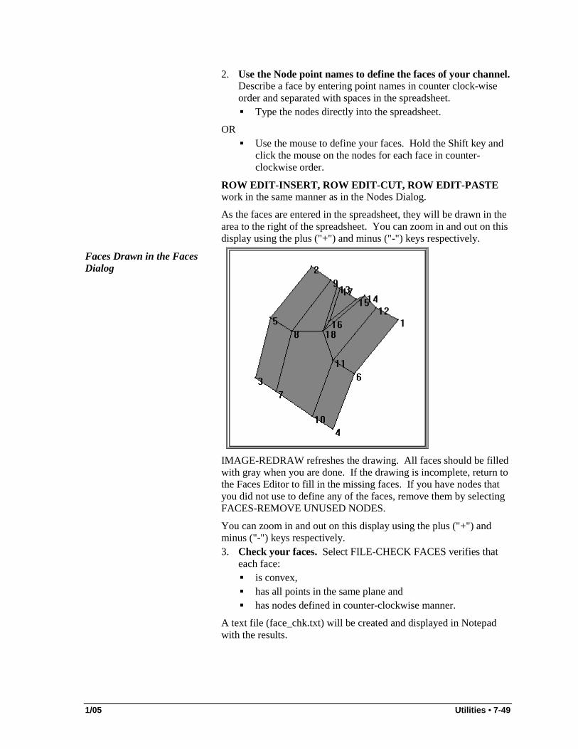
2) Entering Face Data in Advanced Channel Design A face is defined by a closed polygon line, which is represented by a sequence of points.
All faces should be convex to ensure the volume calculation program works correctly. Every non-convex shape can be composed of two or more convex shapes.
.1. Select WINDOW-FACES. The Faces Editor will appear.
Edit Faces dialog
1/05 Utilities • 7-49
2. Use the Node point names to define the faces of your channel. Describe a face by entering point names in counter clock-wise order and separated with spaces in the spreadsheet. ▪ Type the nodes directly into the spreadsheet.
OR ▪ Use the mouse to define your faces. Hold the Shift key and
click the mouse on the nodes for each face in counter-clockwise order.
ROW EDIT-INSERT, ROW EDIT-CUT, ROW EDIT-PASTE work in the same manner as in the Nodes Dialog.
As the faces are entered in the spreadsheet, they will be drawn in the area to the right of the spreadsheet. You can zoom in and out on this display using the plus ("+") and minus ("-") keys respectively.
Faces Drawn in the Faces Dialog
IMAGE-REDRAW refreshes the drawing. All faces should be filled with gray when you are done. If the drawing is incomplete, return to the Faces Editor to fill in the missing faces. If you have nodes that you did not use to define any of the faces, remove them by selecting FACES-REMOVE UNUSED NODES.
You can zoom in and out on this display using the plus ("+") and minus ("-") keys respectively. 3. Check your faces. Select FILE-CHECK FACES verifies that
each face: ▪ is convex, ▪ has all points in the same plane and ▪ has nodes defined in counter-clockwise manner.
A text file (face_chk.txt) will be created and displayed in Notepad with the results.

7-50 • Utilities 1/05
Checking the Faces
Non Convex Shape Error indicates that the face is concave. To correct this, the face must be divided into two or more convex shapes. You can do this by manually editing the faces in the spreadsheet or by using the Split function.
a. Select the offending face in the Face Editor by right clicking the face and selecting Select from the pop-up menu.
b. Right click the selected face and select Split. The program will divide the face.
Note: You should check to be sure that both resulting shapes are now convex. If the original face was particularly complex, you may need to create more than one split to eliminate all concave shapes.
Non-flat Face Error indicates that all the nodes are not in the same plane. The number following the message tells you the distance (in survey units) that the nodes vary. It's up to you how much error your survey will tolerate. You can choose to leave it or correct the node.
Orientation Error means that the nodes were described in clockwise manner. This will not affect the volumes calculations, but when you select WINDOW-3D VIEW, faces with orientation problems will be cross hatched. If you want to correct this, return to the Faces Editor and reverse the order of the nodes for those faces. 4. Use FILE-ADD TOES to add toe lines to your channel.
Adding the Toes

1/05 Utilities • 7-51
a. Enter the nodes at each end of the side of a face where you want to add the toe.
Note: Imagine that you are standing on the first node looking toward the second. The toe will slope toward the left of the line defined by those points so you should keep that in mind as you enter the nodes.
b. Enter the Slope and Top Depth. c. Click [Apply] and the program will compute the size and
position of the toe and assign names to the outside corners. 5. Save your faces temporarily by selecting FILE-SAVE. 6. Return to the ADVANCED CHANNEL DESIGN shell by
selecting FILE-EXIT. 7. Save your Channel File when you are finished by selecting
FILE-SAVE or FILE SAVE AS and naming your file. The data will be saved to the project directory with the CHN extension.
C. Importing Channel Template Information to Advanced Channel Design
1) Creating a Channel File from a Planned Line File in Advanced Channel Design
You can create a Channel File (*.CHN) from a Planned Line File with template information. ADVANCED CHANNEL DESIGN then places a node at each point where the Line File intersects with an inflection point. 1. Create a 3-dimensional Planned Line file. This is typically
done in CHANNEL DESIGN, but may also be created in the LINE EDITOR.
2. In ADVANCED CHANNEL DESIGN, select FILE-LNW to CHN. The LNW to CHN dialog will appear.
LNW to CHN dialog
3. Click [LNW File] and select the Planned Line file from the File
Selection dialog. 4. Click [CHN File] and name the Channel file (include the path)
in the File Selection dialog.

7-52 • Utilities 1/05
Beware! If you select an existing file, it will be overwritten!
5. Modify your template (optional). You can use the inflection point checkboxes to customize the creation of your channel file. This option is useful when you are doing TIN to Channel volumes computations but need separate volumes for certain areas. (For example, you may want only the volume for the left toe.) In this case, select the checkboxes corresponding to inflection points that describe parts of the channel that you want to include. The following table gives you a few examples.
Volumes Area Checked Nodes Left of Toe 1-5 Left of Center 1-6 Center Channel 5-7 Right of Center 6-11 Right Toe 7-11
6. Ignore consecutive, matching Planned Lines (optional). This is done by entering an angle measurement after Remove sections if the intersecting angle is less than… field. There may be several consecutive, parallel or near parallel lines of the same shape in your Line File. If you do not need a separate volume for each section, you can speed the calculations and simplify your report by omitting the lines that are parallel, or nearly so, and have matching shapes.
The angle is measured where two non-parallel lines would intersect if their ends were to extend far enough. (Parallel planned lines do not intersect so the angle would be 0. A value of zero will include all lines from the Planned Line File.) • If the angle created is greater than the measurement
specified, the line will be included in the CHN file. • If the angle created is less than the specified angle, it is close
enough to parallel for your purposes and the line will be omitted.
The first and last line of the Planned Line File will never be omitted. The following figures show the difference in a channel created with a setting of 0 versus a setting of 1 degree.
Creating a Channel File without Near Parallel Sections.
Intersecting Angle = 0 Intersecting Angle = 1
7. Click [OK] and the Channel File will be created and saved to the specified directory.

1/05 Utilities • 7-53
2) Creating a Channel File from a Channel Plan File in Advanced Channel Design
You can create a Channel File (*.CHN) from a Channel Plan File (*.PLN). Channel Plan files are created in CHANNEL DESIGN. They contain all of the channel template information entered in the spreadsheets when you create a planned line file using CHANNEL DESIGN. ADVANCED CHANNEL DESIGN reads the inflection point information and uses it to create the Channel File.
PLN to CHN dialog
1. Select FILE-PLN TO CHN. The PLN to CHN dialog will
appear. 2. Complete the dialog and click [OK]. 3. Click [PLN File] and select the Channel Plan File from which
you want to read the template information. 4. Click [CHN File] and name your new Channel File including
the path to the directory where it will be saved.
Extension: Adds additional faces to cover the specified distance from the toes described in the PLN file. 5. Choose whether to include the center line information. 6. Verify the results in the 3DView window by loading the
resulting file (FILE-OPEN) and taking a look.
Original Channel

7-54 • Utilities 1/05
Original Channel with Extensions
Original Channel with No Center Line
D. Viewing your Channel in Advanced Channel Design
In the Node and Faces Editors, use the Image menu options to adjust the view of your data on your screen. From the ADVANCED CHANNEL DESIGN shell, select WINDOW- 3D VIEW and the View window will display your channel.

1/05 Utilities • 7-55
3D View Window
Use the slides to set the perspective from which you view your design. The top slide rotates the design around centered, vertical axis. A left-hand slide rotates the design around a centered, horizontal axis.
You can adjust the zoom scale and positioning of your display using the Zoom and Pan buttons .
If the contours of your channel are difficult to see, you can accentuate the depth changes by increasing the Z Multiplier and clicking the Redraw button .
3D View with Z Axis Multiplied
E. Exporting Channel files in XYZ Format Once you have created your Channel Template file, you can export the template information in XYZ format using the CHN to XYZ feature found in the File menu. 1. Select FILE-CHN to XYZ and a dialog will appear.
CHN to XYZ dialog
2. the path) by clicking the corresponding button.

7-56 • Utilities 1/05
3. Set the distance that you want between each point in the output file under Spacing.
4. Click [OK]. ADVANCED CHANNEL DESIGN will place points at the requested interval along the outlines of the faces.
CHN File
XYZ File
Resulting XYZ Overlaid on the original CHN
F. Examples in Advanced Channel Design
X Y Z A 500 500 -20 A 600 400 -20 B 700 600 -20 C 600 600 -15 D
Solution: 1. Open the ADVANCED CHANNEL DESIGN program by
selecting UTILTIES-ADVANCED CHANNEL DESIGN. The ADVANCED CHANNEL DESIGN shell will appear.
2. Create the rectangular area. a. Enter your Node data. Open the NODE DIALOG by
clicking WINDOW-NODES, and enter the data points as listed above. Select FILE-SAVE to save the data to temporary memory. Select FILE-EXIT to return to the CHANNEL EDITOR.
Example: Creating a Channel and Adding Toes in ADVANCED CHANNEL DESIGN
Create a simple rectangular face with the coordinates listed below.
Check your faces and correct any errors.
Add Toe lines. On the side defined by nodes “A” to “D” the slope is 1:2 and top depth is 0. On the side defined by nodes “C” to “B” the slope is 1:2 and top depth is 0.
Save your file to DEMO.CHN.

1/05 Utilities • 7-57
Nodes Defined
b. Define your faces. Open the FACES DIALOG by selecting
WINDOW-FACES, and entering the nodes in counter-clockwise order. You may manually type them into the spreadsheet (with a space between each number) or hold Shift while using your mouse to click, in sequence, on the nodes that define each face.
The defined faces draw to the right side of the Edit Faces dialog
c. Save your faces to temporary memory by selecting FILE-
SAVE. d. Check your faces by selecting FACES-CHECK FACES. A
text file will appear that will say "Face No. 1 Non Flat Face Error 5". This means that the points defining the face are not all in the same plane and the distance they are off plane from each other is 5 survey units (feet or meters).
e. Correct the error by returning to the node editor and changing the Z-value for node "D" to –20. After saving the nodes and rechecking the faces, the text file should read "Face No.1 O.K.".
f. Return to the CHANNEL EDITOR by selecting FILE-EXIT. 3. Add the Toes.
a. Select FACES-ADD TOES. The Add Toe dialog will appear.
b. Enter the nodes describing the side of the face to which you want to add the toe. Remember, if you pretend you are looking from the first node to the second, the toe will be constructed to the left.
c. Enter the slope of the toe. d. Enter the depth at the top of the toe.

7-58 • Utilities 1/05
Adding Toes
e. Click [Apply]. The program will calculate the size and
position of the toe, and create and name the outer nodes. f. Repeat the process for the second toe.
4. Save your faces by selecting FACES-SAVE. 5. Return to the ADVANCED CHANNEL DESIGN shell by
selecting FACES-EXIT. 6. Save the Channel File by selecting FILE-SAVE and naming it
"Demo". It will be saved to your project directory with a CHN extension.
You can preview the channel in three dimensions by selecting WINDOW-3D VIEW.
Previewing The Channel in 3D View
Example : Creating a Channel Design using a Planned Line File.
Create a Channel File for use in the TIN Model program using the Black Planned Line File in the B1B project as the source of your channel information. Create it with all of the survey lines included and name it Black0.chn. Create a second Channel File omitting lines with an intersect angle of less than 1 degree and name it Black1.chn.
Solution: 1. Open the B1B project by selecting FILE-OPEN PROJECT and
selecting B1B. 2. Open the ADVANCED CHANNEL DESIGN program by
selecting UTILITIES-ADVANCED CHANNEL DESIGN. 3. Select FILE-LNW TO CHN. The LNW TO CHN dialog will
appear.

1/05 Utilities • 7-59
4. Select your Line File. Click on [LNW File] and select the Black.lnw file in the B1B directory from the File Selection Dialog.
5. Name your Channel File: Type in the path and name your file Black0.chn.
The LNW to CHN Dialog
6. Click [OK] to make the conversion. 7. View your Channel File (optional). 8. Load the Black0.chn file by selecting FILE-OPEN and
choosing it from the File Selection dialog. 9. Select WINDOW-3D VIEW and your Channel File will be
drawn to the screen.
The resulting Black0.CHN File drawn in 3D View
10. Click FILE-EXIT to return to the Main Window. 11. Reopen the LNW to CHN dialog. Change the CHN File Name
to Black1.CHN and the angle value to "1" and click [OK].

7-60 • Utilities 1/05
Setting the Intersect Angle in the LNW to CHN Dialog
12. View the new Channel in the 3D View as you viewed
Black0.chn.
Previewing the new channel.
V. Chart Program The CHART program is used to digitize nautical chart information to enable it to be displayed and plotted inside of HYPACK® MAX.
Note: In order to run this program, you must have a Windows® digitizer driver (such as wintab32.dll) installed for your digitizing table/tablet. These drivers are specific for each table/tablet and are not distributed as a part of HYPACK® MAX.

1/05 Utilities • 7-61
The Chart Window
A. Running the Chart Program The program is quite simple to run. 1. Open the CHART program by selecting UTILITIES-
DIGITIZING-CHART. 2. Register your Chart. 3. Digitize your features. You can control the view of your chart
with the standard zoom features in the CHART menu. You can also re-center your chart on the screen by right clicking on the screen. The CHART program will re-draw the screen, centering the information at the click location.
4. Save your Chart. The resulting chart information is stored to a HYPACK® *.DGW file in your project directory. It is a proprietary ASCII format compatible with HYPACK® MAX and the SURVEY program and can be plotted with the HYPLOT or HYPLOT MAX programs.
B. Registering your Chart 1. Select CHART–REGISTER. 2. Enter the X-Y coordinates for the lower left and upper right of
your chart. You should take care to maximize the separation between these values, as it will improve the accuracy of the digitizing process.
3. Click on the lower left and upper right reference, using the 1st digitizer button. Your chart is now registered.
C. Digitizing your Chart Features 1. Select what item you wish to digitize. Items are grouped in the
following categories.

7-62 • Utilities 1/05
Buoys
Control Points
Installations
Landscape
Lights
Lines

1/05 Utilities • 7-63
Obstructions
Radars
Soundings
Text
Landmark

7-64 • Utilities 1/05
You may pick the desired feature you wish to digitize either by selecting Symbols or by clicking on the icon for each item on the taskbar and then selecting the item from a graphical list. 2. Digitize each location where this feature appears. Click the
1st digitizer button at each location you wish to digitize. 3. Repeat the last two steps for each feature. 4. Save your file by selecting FILE – SAVE AS and naming your
file. The resulting chart information is stored to a HYPACK® *.DGW file in your project directory. This is a proprietary-ASCII file format that can be loaded in the HYPACK® MAX area map, in the SURVEY program and plotted in the HYPLOT program.
Note: At any time, you can save your work by selecting File – Save As. When working on large charts, you should periodically save your work.
D. Editing Chart Features in the Chart Program You can left-click your mouse at the screen location of any symbol to access the feature parameters (X-Y Location, Text attached) or to delete the symbol.
VI. Echogram Program The ECHOGRAM program enables you to manually digitize your echograms. This is sometimes necessary in areas with “liquid mud” or “fluff” where the digitized sounding received from the echogram is not representative of the actual bottom. Using the ECHOGRAM program and a digitizer tablet, you can digitize the depths and their relative fix positions. This information is saved in a *.DEP file. The digitized depth data can then be merged with positions in SINGLE BEAM MAX, using [Merge]. The result is saved to an Edited All format file that has the correct position and depth information.
Note: In order to run this program, you must have a Windows® digitizer driver (such as WINTAB32.DLL) installed for your digitizing table/tablet. These drivers are specific for each table/tablet and are not distributed as a part of HYPACK® MAX. 1. Open the ECHOGRAM program by selecting UTILITIES-
DIGITIZING-ECHOGRAM. 2. Register your echogram on the digitizing tablet.
a. Select CHART–REGISTER CHART. b. Use the 1st digitizer button to click:
! the top-left of your echogram scale (key-line),
! the top right of your digitizer scale (key-line)
! the bottom center of your digitizer scale.

1/05 Utilities • 7-65
3. Set the scale for your echogram by selecting Chart–Scale. Enter the value for the top and bottom of your echogram (where you clicked in step one).
Setting your Scale
4. Reference your event marks.
Entering your fix numbers
a. Enter the value of the first event mark b. Click on each individual event mark c. When you're finished, click the digitizer’s 2nd button.
The screen will draw the event marks as you digitize each one. 5. Working left-to-right, digitize the depth information. You
should click the 1st button of the digitizer tablet at each location where you want to store a depth. The program will store the relative fix location (14.25 = 25% of the distance from event 14 to event 15) in an ASCII file format. When you are finished, click the 3rd button.
6. Indicate whether you want to shift the echogram and continue to digitize or you want to stop and save the results to a *.DEP file. If you shift the echogram, you will need to re-register it on your digitizing tablet.
Details for combining your digitized *.DEP files with position data in the SINGLE BEAM EDITOR program are provided in the SINGLE BEAM EDITOR section of the manual.
VII. Shore Manual The SHORE MANUAL program is used to manually enter shoreline and hydrographic features to a Digitized Shoreline Format (*.DIG) file. These files can be displayed in the HYPACK® MAX for use with the Editor programs in the Preparations menu. They can also be

7-66 • Utilities 1/05
displayed in SURVEY program and can be plotted on the Smooth Sheet in the HYPLOT or HYPLOT MAX program.
Shore Manual Dialog
A. Creating a *.DIG File in Shore Manual 1. Open the SHORE MANUAL program by selecting
UTILITIES-DIGITIZING-SHORE MANUAL. 2. Select FILE-NEW to indicate you are creating a new file. 3. Select the type of object (Shoreline, Rock, Wreck, Buoy, etc)
from the drop-down box accessed under Selected Symbol. 4. Enter the X-Y coordinates of the object selected. 5. Click [Add]. The item will appear in the list on the right-hand
side of the window. 6. Repeat these steps for each point you wish to describe.
Note: If you need to start over, click [Clear] or FILE-CLOSE FILE. Everything listed on the right will be erased. 7. Save your file by clicking FILE-SAVE or FILE-SAVE AS and
naming your file. It will be saved by default, to your project directory, but you may save it elsewhere.
B. Editing your Object List in Shore Manual 1. Select FILE-OPEN and choose the file you wish to modify.
Note: If you have a lengthy list, it may be helpful to sort the items by type. You can sort your list in this way by selecting EDIT-SORT. 2. Click on any entered item you wish to change. That item
information will appear on the left. 3. Edit the item information. 4. Click [Edit]. Your new data will replace the original data for
that item. 5. Remove any unwanted items by selecting the item and clicking
[Delete] or by double clicking the item in the list.

1/05 Utilities • 7-67
6. Save your file. Click on FILE-SAVE and give your file a name using the .DIG extension. Your file will be saved to the project file.
C. Printing your Object List You can print the entries in your file by selecting FILE-PRINT. The Windows® printer dialog will appear for you to send it to print.
VIII. DGW Editor The DGW EDITOR is a simple tool to create a DGW file right in HYPACK® MAX. It includes a large selection of point, line and area objects that you can include in your chart. Once it's finished, the file is saved by default to your project directory and can then be loaded to your project as a background file. 1. Launch the DGW Editor by selecting UTILITIES-
DIGITIZING PROGRAMS-DGW EDITOR. The DGW EDITOR dialog will appear.
DGW Editor
2. Select a feature from the tree view list of features on the left.
The corresponding symbol will appear in the box on the left end of the tool bar.
3. Click the Cursor Icon. The DGW EDITOR dialog will minimize to a button at the lower left of your screen.
4. Use your cursor to mark the location(s) where the selected feature occurs. Several consecutive clicks will create: ▪ One point object for each click. ▪ A line that connects each location. ▪ An area defined by the locations indicated.
Note: You can create multiple separate lines or areas by clicking the Break icon between the last point of one feature and the first point of the next feature of the same type. 5. Restore the DGW EDITOR dialog by clicking on its button. 6. Repeat steps 2-5 until you have described all of the features
you want in your chart.
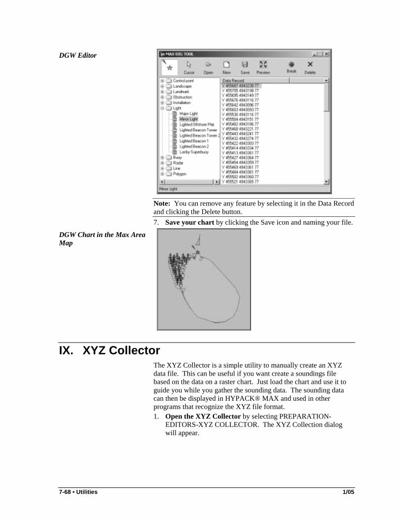
7-68 • Utilities 1/05
DGW Editor
Note: You can remove any feature by selecting it in the Data Record and clicking the Delete button. 7. Save your chart by clicking the Save icon and naming your file.
DGW Chart in the Max Area Map
IX. XYZ Collector The XYZ Collector is a simple utility to manually create an XYZ data file. This can be useful if you want create a soundings file based on the data on a raster chart. Just load the chart and use it to guide you while you gather the sounding data. The sounding data can then be displayed in HYPACK® MAX and used in other programs that recognize the XYZ file format. 1. Open the XYZ Collector by selecting PREPARATION-
EDITORS-XYZ COLLECTOR. The XYZ Collection dialog will appear.

1/05 Utilities • 7-69
XYZ Collection Dialog
2. Double click on the area map at each location where you want
soundings.
Note: The depth defaults to 0.00, but if you have several locations with equal depth values. Set the depth first, then double click each location. Each location will be assigned the same Z. It could save you time over setting each individually. 3. Enter depths for each pair of X-Y coordinates by selecting the
X-Y pair, entering a value in the Z field and clicking the check button (or hit Enter).
4. Save the file by selecting FILE-SAVE and naming the file. The file will be saved, by default, to the project's Sort directory.
To delete any unwanted soundings in the file select the file to be deleted and click the exclamation icon on the right.
To display this file: • In the XYZ COLLECTOR by checking Display Soundings. • In HYPACK® MAX by loading the file as you would any
sounding file. (Right click on the sort directory, select Add File and choose your XYZ file from the file selection dialog.)
X. Sounding Adjustment The SOUNDING ADJUSTMENT program reads edited All format files and applies sound velocity corrections to them. These corrections are based on where Depth 1 falls in the Data Corrections Table and the data that you enter into it. The program adds the "fixed" corrections (not interpolated values) to the current sound velocity values in the data. 1. Select PROCESSING-SOUND VELOCITY-SOUNDING
ADJUSTMENT. The Data Corrections Table will appear.

7-70 • Utilities 1/05
Depth Corrections Table
2. Enter the depths and adjustment values to the Data
Corrections Table. In this example, depths less than 40 will receive the sound velocity correction of 0.40, depths from 40-60 will receive the correction of 0.60, etc.
3. Save your Depth Corrections Table by selecting FILE-SAVE or FILE-SAVE AS and giving it a name. Your data will be saved to your project directory with a .DCT extension.
4. Apply the corrections to your data by selecting FILE-GENERATE CORRECTIONS. Select the edited All format files you wish to correct from the list in the file manager. The corrections will be automatically made.
If you are correcting single beam data, you can see the results by viewing your data in SINGLE BEAM MAX.
XI. Data Adjustments Program The DATA ADJUSTMENTS program is used to make changes to Raw Data Files collected in the SURVEY program. The program reads your raw data files, either one-by-one or via a catalog (*.LOG) file. It creates new data files in the same directory that it reads from, and saves each file with a new extension. It also creates a new catalog file (*.LOG) automatically, using the extension as the root of the catalog name.
Note: It will only work with RAW format files. Don’t try it with ALL format or XYZ format data.
A. Running Data Adjustments 1. Verify the geodetic parameters in the GEODETIC
PARAMETERS program as DATA ADJUSTMENTS will use these.
2. Select UTILITIES-FILE WORK-DATA ADJUSTMENTS. The Data Adjustments dialog will appear.

1/05 Utilities • 7-71
DATA ADJUSTMENT Window
3. Check the check boxes for the data you need to adjust. 4. Enter the adjustment value for each item. 5. Set your new File Extension. It defaults to ZZZ but you can
enter any alphanumeric combination. 6. Select the data you wish to adjust by selecting FILE-OPEN
FILE and choosing the file from the file selection dialog. You can choose a catalog file or an individual file.
7. Adjust the data by selecting FILE-ADJUST. The data will be adjusted according to your settings in the dialog and the results will be saved with the new extension to the same folder.
B. Data Adjustment Items You can adjust the following items:
Positions • Add an offset to the X or Y coordinates. • Adjust the time stamp of the position records.
Gyro • Adjust the gyro angle (in degrees). • Adjust the time stamp of the gyro records.
Heave-Pitch-Roll • Adjust the heave, pitch or roll (or more than one of these). • Adjust the time stamp of the depth records.
Depths • Adjust the depth by multiplying by or adding a user-defined
constant. • Adjust the time stamp of the depth records.
Recalculate Range-Azimuth

7-72 • Utilities 1/05
• Re-calculate your range-azimuth data. It requires the old station X-Y and reference azimuth and the new station X-Y and reference azimuth.
• Adjust the time stamp of the position data.
XII. Manual Entry Program Manual Entry enables you to create your own depth readings along a planned line file and store it in a HYPACK® ALL format file. This utility was designed for you to enter tag-line distance and depth information. 1. Start the program by selecting UTILITIES-FILE WORK-
MANUAL ENTRY or by clicking on the File Work icon and selecting Manual Entry from the drop-down box. The Manual Entry window appears.
2. Enter Line Information: Choose to use a pre-existing planned line file or to manually create the start and end X and Y coordinates as you go. ▪ FROM FILE enables the Line File information.
Manual Entry Dialog—File Mode
i. Select your Line File. Click on FILE NAME then
[Browse] and select the line file for which you want to create data. The remaining Line Information will automatically be displayed.
ii. Choose which line in the file you want to work with.
iii. Enter the additional sounding information in the spreadsheet.
iv. Save your file. Click on FILE-SAVE and name your file. It will be saved to the edit directory.
▪ MANUALLY disables the Manual Line information. You must enter the Start and End X and Y coordinates for yourself. Otherwise it works the same way as the From File method.
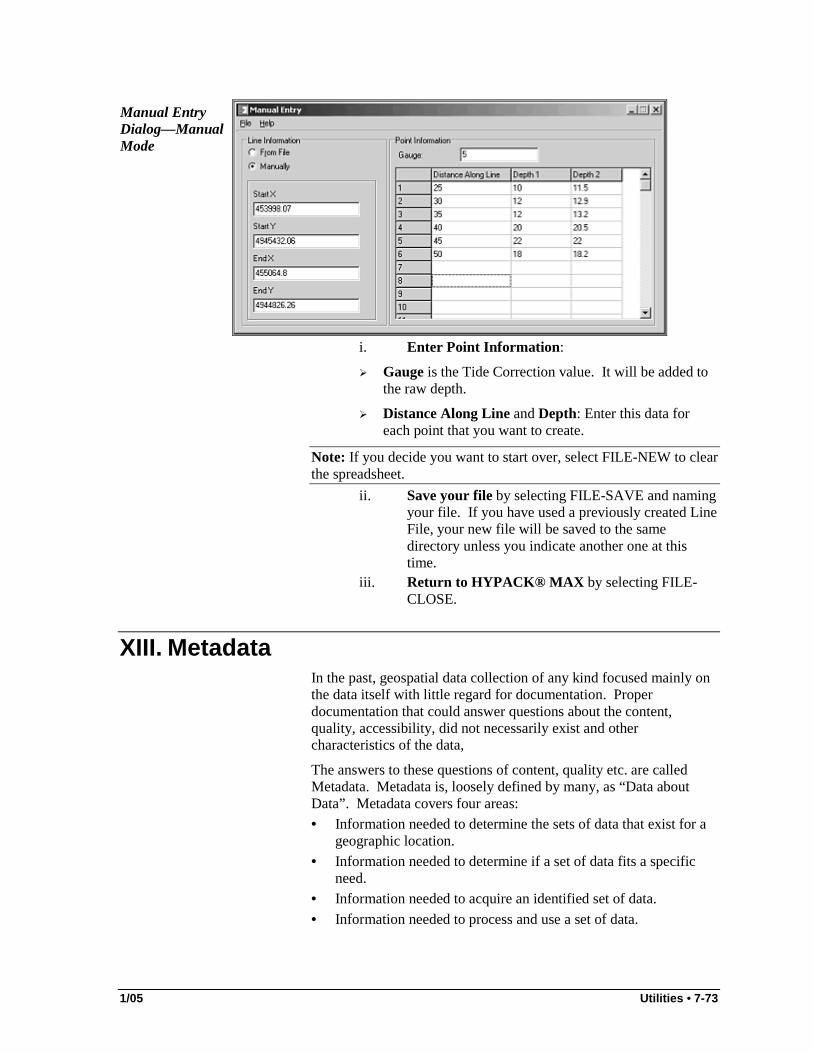
1/05 Utilities • 7-73
Manual Entry Dialog—Manual Mode
i. Enter Point Information:
! Gauge is the Tide Correction value. It will be added to the raw depth.
! Distance Along Line and Depth: Enter this data for each point that you want to create.
Note: If you decide you want to start over, select FILE-NEW to clear the spreadsheet.
ii. Save your file by selecting FILE-SAVE and naming your file. If you have used a previously created Line File, your new file will be saved to the same directory unless you indicate another one at this time.
iii. Return to HYPACK® MAX by selecting FILE-CLOSE.
XIII. Metadata In the past, geospatial data collection of any kind focused mainly on the data itself with little regard for documentation. Proper documentation that could answer questions about the content, quality, accessibility, did not necessarily exist and other characteristics of the data,
The answers to these questions of content, quality etc. are called Metadata. Metadata is, loosely defined by many, as “Data about Data”. Metadata covers four areas: • Information needed to determine the sets of data that exist for a
geographic location. • Information needed to determine if a set of data fits a specific
need. • Information needed to acquire an identified set of data. • Information needed to process and use a set of data.

7-74 • Utilities 1/05
To provide compilers and users of geospatial data with a common set of terminology, the FGDC (Federal Geographic Data Committee) created and approved the Content Standards for Digital Geospatial Metadata.
The FGDC standard is broken down into seven main sections: Identification Information
Basic information about the data set.
Data Quality Information
A general assessment of the quality of the data set.
Spatial Data Organization
The mechanism used to represent spatial information in the data set
Spatial Reference Information
The description of the reference frame for, and the means to encode, the coordinates in the data set.
Entity and Attribute Information
Information about the information content of the data set, including the entity types, their attributes, and the domains from which attribute values may be assigned
Distribution Information Information about the distributor of and options for obtaining the data set.
Metadata Reference Information
Information on the how current the Metadata information is, and the possible responsible party.
All sections and any fields in a section of the standard are either Required, Optional, or required where applicable. To complete a section, all of the required fields under that section must be completed.
In the case of the Standard as a whole, sections 1 and 7 must be “completed” for the file to be compliant with the FGDC standard.
Metadata can be created in HYPACK® with the Metagen program. Metadata created with Metagen adheres to the FGDC standard.
A. Creating Metadata 1. Start the Metadata program by selecting UTILITIES-FILE
WORK-METADATA. 2. Enter the data in the tree items necessary for your report.
Identification and Metagen Reference tree items are the minimum required for creating a Metagen project. Complete also any others that are applicable to the type of report you are creating.
3. Build your Metadata report by selecting PROJECT-BUILD METADATA FILE.
4. Save your data to *.GEN and *.MET files.
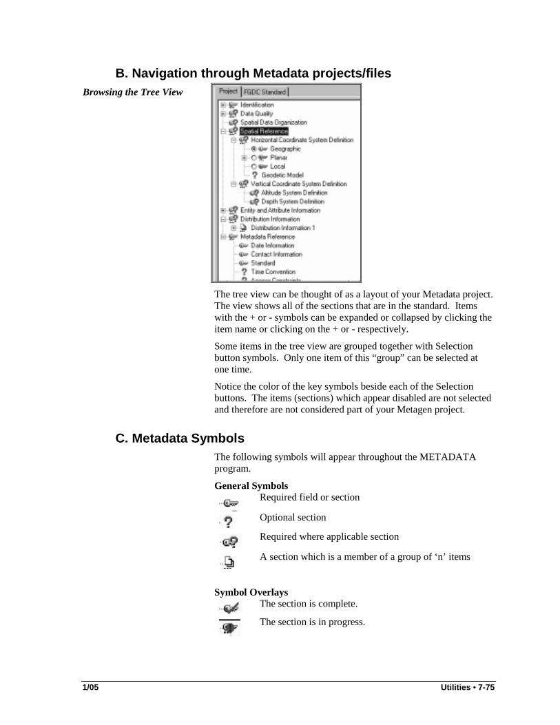
1/05 Utilities • 7-75
B. Navigation through Metadata projects/files Browsing the Tree View
The tree view can be thought of as a layout of your Metadata project. The view shows all of the sections that are in the standard. Items with the + or - symbols can be expanded or collapsed by clicking the item name or clicking on the + or - respectively.
Some items in the tree view are grouped together with Selection button symbols. Only one item of this “group” can be selected at one time.
Notice the color of the key symbols beside each of the Selection buttons. The items (sections) which appear disabled are not selected and therefore are not considered part of your Metagen project.
C. Metadata Symbols The following symbols will appear throughout the METADATA program.
General Symbols
Required field or section
Optional section
Required where applicable section
A section which is a member of a group of ‘n’ items
Symbol Overlays
The section is complete.
The section is in progress.

7-76 • Utilities 1/05
Symbol Modifiers
The section is disabled.
The section itself has no properties.
Other Symbols
Selection Button - selected
Selection Button - unselected
Note: The used in ‘Symbol Modifiers’ serves only as an example. All of the other symbols may be modified in the same manner.
D. Entering Data in your Metadata Report Every item in the tree that does not have the "..." modifier on the item’s symbol, has a property dialog associated with it. To reach the property dialog for any of these items simply double click on the item in the tree or right click on the item to bring up the pop - up menu and then select Properties. (The pop-up menu does not come up if you have a dialog already displayed.)
Choosing to view the Properties

1/05 Utilities • 7-77
“Time Period of Content” dialog from the “Identification” Section
All data entry is done in the property dialogs.
The three buttons on the bottom of every property dialog are always the same ( [OK], [Cancel], [Apply]), however, the contents of each dialog will change according to the item you are on in the tree. The three “standard” buttons always mean the following: • [OK]: Save changes and close dialog. • [Cancel]: Close dialog discarding any changes. • [Apply]: Save changes without closing dialog.
Notice at the top of the ‘Date’ field there is a key symbol. This indicates that the ‘Date’ field is a required entry field. After each of the required entry fields is complete, the tree-item selected for edit is complete.
After saving changes to our data in a property dialog, you may notice changes to the tree item we had selected for editing. If the minimum number of required entries for the current tree - item (indicated by the key symbol) are complete, the symbol for the current tree item will appear with a check mark over it. If some, but not all, of the required entries for the current tree item are complete, then the current tree item will appear with a red dot over it.
These changes will reciprocate up the entire tree. (In some cases the ‘Status’ change of one tree item will cause changes in other items above it.) Notice in the previous figure, the changes in the tree after saving changes to our property dialog. • The ‘Citation’ and ‘Description’ items under ‘Identification’ in
the tree have the Completed (Check Mark) symbol over it. • The ‘Identification’ item in the tree has the In Progress (Red
Dot) symbol over it.

7-78 • Utilities 1/05
Since the ‘Citation’ and ‘Description’ items are the only items under ‘Identification’ that have been completed the ‘Identification’ item is clearly ‘In Progress’.
E. Building the *.MET file and Saving the *.GEN file Building a *.MET file is only possible when you have completed at least the ‘Identification’ and ‘Metadata Reference’ sections. They are complete when the tree view shows red checks on those sections.
A Complete Project
When these conditions are met you will see both [Build All] and PROJECT-BUILD METAFILE become active. (Notice in the Tree view, that both of the required tree-items are complete.)
The Build All button (left) and the Build Metafile option under the Project menu (right)
*.GEN files are Metagen Project files. This is the file you save while in the Metagen program. It is NOT compliant to the FGDC standard.
*.MET is a Metadata file. This is the Metadata file you build while in the Metadata program. It is a formatted ASCII text file and is compliant to the FGDC standard. A portion of a *.MET file appears as follows:
Identification_Information:
Citation:
Citation_Information:
Originator: David Hodges(Ed.)
F. Saving a Metadata project At any time when the Metagen program is running, you may save the current Metagen project by selecting FILE-SAVE or by clicking the Save icon. You can save the current project under a new name by selecting FILE-Save As or click the Save As icon. The project will be saved with the *.GEN extension to the project directory.
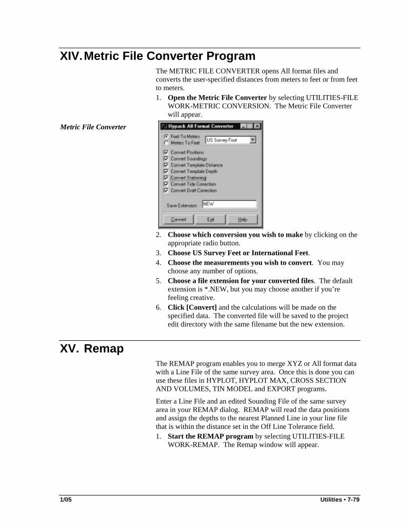
1/05 Utilities • 7-79
XIV. Metric File Converter Program The METRIC FILE CONVERTER opens All format files and converts the user-specified distances from meters to feet or from feet to meters. 1. Open the Metric File Converter by selecting UTILITIES-FILE
WORK-METRIC CONVERSION. The Metric File Converter will appear.
Metric File Converter
2. Choose which conversion you wish to make by clicking on the
appropriate radio button. 3. Choose US Survey Feet or International Feet. 4. Choose the measurements you wish to convert. You may
choose any number of options. 5. Choose a file extension for your converted files. The default
extension is *.NEW, but you may choose another if you’re feeling creative.
6. Click [Convert] and the calculations will be made on the specified data. The converted file will be saved to the project edit directory with the same filename but the new extension.
XV. Remap The REMAP program enables you to merge XYZ or All format data with a Line File of the same survey area. Once this is done you can use these files in HYPLOT, HYPLOT MAX, CROSS SECTION AND VOLUMES, TIN MODEL and EXPORT programs.
Enter a Line File and an edited Sounding File of the same survey area in your REMAP dialog. REMAP will read the data positions and assign the depths to the nearest Planned Line in your line file that is within the distance set in the Off Line Tolerance field. 1. Start the REMAP program by selecting UTILITIES-FILE
WORK-REMAP. The Remap window will appear.

7-80 • Utilities 1/05
Remap Dialog
2. Fill in the fields in the dialog.
▪ New Planned Line File is the line file of your survey area. It may be created in the LINE EDITOR or in the CHANNEL DESIGN program.
Planned Line File
▪ Existing Data Source File is your *.XYZ or *.LOG File
that you wish to merge with the line file. If you were to view it in the Main window of HYPACK® MAX, it would appear as a solid mass of data points.

1/05 Utilities • 7-81
The Original Data Set
▪ New Data Extension is used to specify the extension that
will be appended to your merged data file. ▪ Off Line Tolerance is the largest allowable distance
between the position of the data points and a planned line. If there is no planned line within this distance from a data point it will be disregarded.
▪ The Survey Date will be written to the header of the new files.
3. Click on [Remap] and the program will process your data, save the results to the project's edit directory, and tell you when it has finished successfully.
4. Click [OK] to return to the Main window.
If you view your new data set you will see that the points are now clustered around the planned lines.
The resulting Data Set
For a more detailed view of the results, zoom a window so you can see the individual soundings clustered around the selected lines.

7-82 • Utilities 1/05
The first two lines of the Line file after REMAP
XVI. Pathfinder Program The Pathfinder program reads the positions from the user-selected sounding files and creates a Planned Line file (*.LNW) that defines the track line of the survey boat. 1. Select UTILITIES-FILE WORK-PATH FINDER. The
Pathfinder dialog will appear. 2. Select SETUP and a secondary dialog will appear.
Setup Dialog
3. Select the sounding catalog file. 4. Name the resultant Line file. 5. Define the number of line segments to be used. The more
segments, the more closely the LNW File will be able to match a curving track line. There is no maximum number of segments you can use. It's a matter of trial to determine the optimal number of segments to use for each situation.
6. Click [OK] to return to the Pathfinder window. 7. Select RUN. The resulting line file will be drawn to the
Pathfinder window and saved to the specified file and location.
Note: If you have chosen a catalog file, each line in the file will be drawn individually and you will be asked if you wish to continue to the next line.

1/05 Utilities • 7-83
Sample Results of Running PATHFINDER
If you are not happy with the results, re-open the setup dialog and edit the input.
XVII. Merge XYZ The MERGE XYZ program enables you to add XYZ data to edited All format files. The program creates a new catalog of All format files that include the data from the XYZ files and have a user-defined extension. The new catalog file will be named with the original catalog name with the new tag appended. For example, "catalog.log" will become "catalognew.log". 1. Select UTILITIES-FILE WORK-MERGE XYZ and the
Merge XYZ dialog will appear.
Merge XYZ dialog
2. Enter the two file sets that you want to combine. You may
type the path and file name directly into the field or click the corresponding […] buttons to browse for them.
3. Define the tag for your new data files.

7-84 • Utilities 1/05
4. The Offline Tolerance is the largest allowable distance between the position of the XYZ data points and the survey line information in the All format file. If there is no planned line within this distance from a data point it will be disregarded.
Note: If your XYZ data extends beyond the end of the survey line, the program will calculate a theoretical extension of the survey line and calculate the offline tolerance based on this extension. 5. If you want to invert your depths check Yes under Negate Z-
values. 6. Click [Go] and the new files will be created and saved to the
project's Edit directory.
XVIII. ADCP Logger The ADCP DATA LOGGER collects and provides real time displays of water current data (magnitude and direction) from RD Instruments' Workhorse Rio Grande ADCP device with position, heading and depth data from HYPACK® SURVEY. It runs simultaneously with the SURVEY program and logs data whenever the SURVEY program is in logging mode. Real-time graphic displays enable you to monitor your current status (no pun intended).
ADCP Logger
The data is stored to the project directory in an ADCP subdirectory. The data files have the same root name as the corresponding Survey files and have an ADCP extension. They are also listed in the adcplogger.log catalog file. You may, in addition, store your data to the same directory in RD Instruments' *r.000 format by selecting Create Raw Ensemble File in the Advanced Options dialog.
The ADCP format file includes all of the ensemble data as found in the r.000 files, as well as position (in local coordinates), depth and heave, pitch and roll information from SURVEY.

1/05 Utilities • 7-85
These files can be read into the ADCP PROFILE program to create cross section views of your data and textual discharge reports. They can also be converted to DXF format, in the ADCP TO DXF program to be used as background files in HYPACK® MAX, to be plotted in one of the HYPLOT programs, or to be imported into other packages such as AutoCAD.
A. ADCP LOGGER Procedure The ADCP LOGGER provides you with a choice of operation modes. • Regular Mode synchronized logging of ADCP data with
HYPACK® MAX SURVEY. • Listening Mode enables you to initiate data logging through the
OEM software and still use the ADCP LOGGER features. You will need a "Y" cable to connect the ADCP device to both the port for the OEM software and the port for the HYPACK® ADCP LOGGER.
The procedures differ a little according to which mode you choose. In either case, the ADCP LOGGER does not log the data to the data file until you start logging in the SURVEY program. You can confirm the logging state by looking at the bottom right corner of the ADCP LOGGER window.
1) Running ADCP LOGGER in Regular Mode 1. Start the ADCP LOGGER by selecting UTILITIES-ADCP-
ADCP LOGGER in the HYPACK® menu or OPTIONS-SHARED MEMORY-ADCP LOGGER in the Survey menu.
2. Select the mode of operation. The first time you launch this program, "No Device Connection Exists." will appear in the log display area.
3. Connect to the ADCP device. 4. Test the ADCP connection. 5. Open the plan file that has been created using RDI software.
The extension should be .CGF, .WHP or .WRC. 6. Deploy the plan file. The ADCP LOGGER sends commands
from the plan file to the device. (You can see them in the log display window.)
7. End ADCP data logging in the ADCP LOGGER by selecting FILE-STOP ADCP.
2) Running ADCP LOGGER in Listening Mode 1. Start the ADCP LOGGER by selecting UTILITIES-ADCP-
ADCP LOGGER in the HYPACK® menu or OPTIONS-SHARED MEMORY-ADCP LOGGER in the Survey menu.
2. Select the mode of operation. The first time you launch this program, "No Device Connection Exists." will appear in the log display area.

7-86 • Utilities 1/05
3. Connect to the ADCP device. 4. Initiate the ADCP data logging through the OEM software. 5. Initiate ADCP data reading in the ADCP LOGGER by selecting
FILE-READ ENSEMBLE DATA. The data should scroll through the ADCP LOGGER window.
6. End ADCP data reading in the ADCP LOGGER by selecting FILE-STOP READING DATA.
B. Connecting your ADCP Device Once you have connected the device to the serial port via cables, you must tell the program to which port it is connected. 1. Select FILE-CONNECT and the Connect To dialog will
appear.
ADCP Connect To Dialog
2. Click [Change Settings] and the Serial Port Settings dialog will
appear for you to define your settings.
Serial Port Settings Dialog
3. Define your settings according to the port where your cable is
connected and the recommended settings from your device manual.
4. Click [OK] to return to the Connect To dialog.
Note: It is not necessary to add the ADCP device in the HYPACK® HARDWARE program.
C. Testing the ADCP Connection Once you have connected the ADCP device to your serial port, if you are running in Regular Mode, you should run the Break Test.

1/05 Utilities • 7-87
In the Connect To dialog, click [Test Connection]. You should see the ADCP response messages in the Log display area of ADCP LOGGER program.
If the connection fails, check the cable connection and serial port settings and try again.
When the Break Test succeeds, click [OK] to return to the ADCP LOGGER.
After you have performed the Break Test successfully, it is recommended that you also test additional commands used with the device. 1. Select FILE-TEST ADCP. The ADCP Test dialog appears. 2. Click [Test ADCP]. ADCP LOGGER now tests the ADCP
device by sending BREAK, PA, OL, PSO and CZ commands to it. The exact sequence and the set of these commands can change and is documented on the dialog itself at the bottom. You should see the ADCP response messages in the Log display area of ADCP LOGGER program.
D. Opening the Plan File in the ADCP Logger Before you open a plan file for deployment, you must have already prepared the plan file using one of the RDI software products 1. Click on the menu FILE-OPEN PLAN FILE. A confirmation
dialog appears that shows you the name of the current plan file and asks you whether you want to continue.
2. If you have prepared the plan file, click on [Yes]. An File Selection dialog appears.
3. Select the plan file that you have prepared and click [Open]. Note that the plan file should have the file extension whp, cfg or wrc. ADCP LOGGER now displays a message in the Log display area that confirms that the plan file is selected and is ready for deployment. The status bar at the bottom also shows a similar message.
E. Deploying the Plan file in ADCP LOGGER Select FILE-DEPLOY. ADCP LOGGER will send the commands from the current plan file to the ADCP device. You can see messages in the Log display area as each command in the Plan file is sent to the device.
As the data starts coming from the ADCP device, you should see the ensemble data being received and displayed in the Log display area.
Note: The ADCP LOGGER does not log the data to the data file until you start logging in the SURVEY program. You can confirm the logging state by looking at the bottom right corner of the ADCP LOGGER window.

7-88 • Utilities 1/05
If you open one or more data monitoring views, you can also see the data being received in various pictorial or textual views.
To deploy a different Plan File: 1. Select FILE-STOP ADCP. The ADCP LOGGER stops the
ADCP device by sending a break command to it. If data logging is going on, ADCP LOGGER will ask for confirmation before the stop operation.
2. Select FILE-OPEN and select a new Plan File.
F. Logging ADCP Data Logging is controlled by the SURVEY program's logging commands. It can be done in either Regular or Listening Mode.
Begin Logging data to the data file by selecting FILE-START LOGGING in SURVEY. The logging status is displayed at the bottom right corner of the ADCP LOGGER window.
Pause Logging by selecting FILE-PAUSE LOGGING.
Restart Logging by selecting FILE-RESUME LOGGING.
End Logging by selecting FILE-END LOGGING in the SURVEY program.
G. Windows in ADCP LOGGER The ADCP LOGGER has several windows available for you to view your data as it is logged. You can select which windows you want to see using View menu selections.
Display settings may be customized by selecting TOOLS-OPTIONS in the main window or by selecting SETTINGS in the individual windows.
1) ADCP LOGGER Window Start the ADCP LOGGER by selecting UTILITIES-ADCP-ADCP LOGGER in the HYPACK® MAX menu. The ADCP LOGGER window will appear.

1/05 Utilities • 7-89
ADCP LOGGER
This is the main control window of the ADCP LOGGER program. From this window you can: • Choose a Configuration File • Connect to the ADCP • Deploy the ADCP • Choose View Windows
Five Alarm buttons across the top of the window indicate signal loss when they turn red. They can also be used to determine the content of the scolling display. You can view Navigational, Heading, Pitch/Roll or ADCP data, each individually by clicking the corresponding button, or you can view them all by clicking [System].
2) ADCP LOGGER Tabular View The Tab View is a scrolling, user-configurable view of your data.
Tabular Display
The first time you use this window, you must select the data you want displayed. This configuration will be the Tabular Standard.
You can also create and customize additional displays, saving each configuration for future use. 1. Select SETTINGS-CHANGE NAME and name your new
configuration.

7-90 • Utilities 1/05
2. Customize your display listing by selecting SETTINGS-CONFIGURE and changing your settings in the Tabular Display dialog.
Tabular Display Settings Dialog
3. Check the Velocity, Intensity and Correlation display choices
to be displayed. You can also choose to display which bins will be displayed from each ensemble. ▪ Bin Numbers From specifies a range of bin numbers. The
interval number tells the program to show bins spaced at even intervals throughout the range. For example, an interval of 3 tells the program to display every 3rd bin in the specified range.
▪ Bin Numbers enables you to specify individual bins or bin ranges to be displayed from each ensemble. List the bins in a comma delimited listing. The listing may include individual bins as well as ranges (ie. 5, 25-43, 52-81,100).
Note: The same dialog may be accessed in the Tabular tab of the ADCP LOGGER Options dialog.
3) ADCP LOGGER Velocity Profile Windows The Velocity Profile windows graph current velocity over a user-specified depth range against "Ensemble Time" or "Ensemble Number". Choose currents moving "East-West", "North-South" or "Vertically" or the "Error Velocity".

1/05 Utilities • 7-91
East-West Velocity Profile
1. Set the X axis units. In the LOGGER window, select TOOLS-OPTIONS. On the Profiles Tab, choose either Ensemble Time or Ensemble Number.
Profiles Tab
2. Set color options by selecting SETTINGS-COLOR SETTINGS
and configuring the color table. (Details on working with the Color Table are found in the Introduction chapter under "Sounding Color Settings in Hypack Max".)
Profile Color Settings
3. Set the Depth Range by selecting SETTINGS-DEPTH
SETTINGS. The Depth Range dialog will appear.

7-92 • Utilities 1/05
Profile Depth Settings
Show as Bad Data Below Bottom automatically displays all readings at depths greater than those read by the echosounder as bad.
Bottom Detected By options determine the source of the bottom profile information. • Bottom track draws data from the ADCP device. • Echosounder uses depth information from the Survey program.
Depth to be Viewed on Screen sets the depth range of the profile. You can enter a depth range or click [Full Range] to auto-adjust the size of the graph to accommodate all soundings.
Keep this window Always on Top by selecting this option in the Settings menu.
4) ADCP LOGGER Intensity Profile Window The Intensity Profile window shows the intensity of the return signal at increasing depths. There are five Intensity Profile windows. One for each beam (1-4) individually and one that averages the values of all of the beams.
Depth and Color settings, as well as Units and Always on Top status are defined in the same way as for the Sound Velocity Profile.

1/05 Utilities • 7-93
Intensity Profile Window
5) ADCP LOGGER Transect Vector Window The Transect Vector window is a 2D display of the track line and water current vectors. Start and End Logging status is shown with green and red dots respectively.
You can adjust the range of the graph by dragging the edges of the window to resize it.
Transect Vector Window
6) ADCP LOGGER Magnitude Direction Profile The Magnitude Direction Profile is a real-time display of data from a user-specified bin. It includes: • Ensemble date, time and number • Velocity and direction for the bin • Boat heading

7-94 • Utilities 1/05
Magnitude Direction Profile
Select SETTINGS and the Magnitude Direction Profile Settings dialog will appear.
Magnitude Direction Profile Settings
Bin Choices defines the range of bins (by number) to be represented in the window. Each bin will be represented by one concentric circle on the graph. Note these values should be no greater than the Total Bins displayed at the top of the dialog.
Color Palette shows the current color of the data line. [Change]
Display Bin Number tells the program to label the bin lines at the user-defined interval. For example, if this option is checked and 3 is entered as the interval, every 3rd circle will be labeled with the bin number.
Display Magnitude tells the program to label the magnitude at the user-defined interval. In this case, if this option were checked and 3 entered, the magnitude will be displayed for every third bin in the range.

1/05 Utilities • 7-95
7) ADCP LOGGER Data Displays The Data Display provides the most recent readings from the ADCP LOGGER program. View the Data Display by selecting VIEW-DATA DISPLAYS and choosing the name of the desired configuration.
Logger Data Display
The first time you use this window, you must select the data you want displayed. This configuration will be the Custom Standard.
You can also create and customize additional displays, saving each configuration for future use. 1. Select SETTINGS-CHANGE NAME and name your new
configuration.
Logger Data Display
2. Customize your display listing by selecting SETTINGS-
CONFIGURE and listing your desired items in the Items Displayed list. Move items between the Items Available and Items Displayed lists with the arrow keys. (The double arrow keys move the entire list.)
8) ADCP LOGGER Hypack Information Window The HYPACK® Information window displays the most recent readings from the HYPACK® SURVEY program. This display has only the standard configuration. If you need to view additional

7-96 • Utilities 1/05
information from SURVEY, the Data Display window in SURVEY may be customized for your purposes.
HYPACK® Information Window
H. ADCP LOGGER View Options You can define settings for each window by selecting TOOLS-OPTIONS. A tabbed dialog will appear for you to make your choices.
1) ADCP LOGGER Units Options The Units Tab enables you to select the units of measure in the various displays.
Units dialog
Range defines the units for distances in the data views.
Velocity defines the units for the velocity display in the data views
Magnitude Stick defines the scale for relating magnitude.
2) ADCP LOGGER Reference Options The Reference options refer to the Velocity Profile views. You can choose to reference the velocity data to the ADCP bottom track, to HYPACK's navigational data, or to neither.

1/05 Utilities • 7-97
Reference Options
None shows raw data from the ADCP.
Bottom Track shows velocities corrected for the motion of the ADCP based on the ADCP's bottom track data.
Navigation shows velocities corrected for ADCP motion based on navigation data. (Not yet implemented.)
3) ADCP LOGGER Data Display Options The Data Display Tab displays the same dialog as using the Settings menu in the Data Display window.
List your desired items in the Items Displayed list in the Data Display Configuration Tab. Move items between the Items Available and Items Displayed lists with the arrow keys. (The double arrow keys move the entire list.)
4) ADCP LOGGER Tabular Display Options The Tabular Tab displays the same dialog as using the Settings menu in the Tabular window. Information about these options may be found under "ADCP LOGGER Tabular View".
5) ADCP LOGGER Profiles Options The Profiles tab defines the X axis units in the profile windows. You can choose to graph the ADCP data against the Ensemble Time or Ensemble Number.
Defining the Profile X-axes

7-98 • Utilities 1/05
6) ADCP LOGGER Advanced Options The Advanced tab enables you to: • Choose to create a standard ADCP format file (*r.000), in
addition to the Hypack® *.ADCP file using the same ADCP data. • Choose to use the heading from HYPACK® SURVEY rather
than the heading from the ADCP device.
Raw Ensemble File Option
7) ADCP LOGGER Log Into File Options The Log into File option enables you to log user-selected items from the data into an ASCII text file. This text file is for your future reference only. You can print copies, but it has no further use in the ADCP or HYPACK® software.
Configuring the Textual Log File
1. Select this option by checking the Log Into File box. 2. Specify the path and text file name by clicking [Browse] and
selecting the path and file name. Accepting the default settings,

1/05 Utilities • 7-99
the data will be saved to the ADCP folder in your project under the name LogOutput.txt.
3. Choose when to log data to your file--all the time or only when SURVEY is in Logging mode.
4. Configure your output file. 5. Select the items to be output in each record using the left and
right arrow keys to move them to the Logged Data list. The items will be output in the same order as they are listed. If you want to shift an item's position in the Logged Data list, select it and use the up and down arrow buttons to reposition it in the list.
6. Specify the number of characters for each item by selecting it, typing a number in the Width field and clicking [Apply].
7. Specify the Bin range from which to log data. 8. Click [OK]. You can preview your data string near the bottom of the dialog.
XIX. ADCP Profile The ADCP PROFILE program reads ADCP files and HYPACK® All format files and displays color-coded flow data with the channel cross section. It can send print or plot the resulting cross section graphs. The ADCP PROFILE program also creates textual discharge reports that you can save and print.
A. ADCP Profile Procedure 1. Start the program by selecting UTILITIES-ADCP-ADCP
PROFILE. The ADCP PROFILE window will come up with a series of tabbed dialogs.
2. Load your data files. Select FILE-OPEN and select file from the File Select dialog. You can load a catalog file from your Edit directory and the corresponding ADCP files will load automatically.
3. Enter the information in each tab. ▪ The Surveys Tab requires information regarding your
survey data. ▪ The Graph Options Tab defines how your profiles will be
displayed. Here, you make choices about the appearance of the grid, labels and annotations.
▪ The View Tab enables you to preview the cross section graphs. You may also adjust the scale and segment of the cross section to include in the graph.
▪ The Print Tab enables you to setup and print the cross section graphs.
▪ The Discharge Tab displays an online preview of your discharge calculations.

7-100 • Utilities 1/05
B. Surveys Tab in the ADCP Profile Program Once you start the ADCP PROFILE program, the program’s Surveys Tab will appear. This spreadsheet enables you to enter your survey and ADCP data. The files will be listed in the column in the same order that they are listed in the catalog file.
Channel Templates, also known as cross section design templates are based upon the geometry of the channel. They are included in 3-dimensional planned line files created in the LINE EDITOR or in CHANNEL DESIGN. The Survey program logs the template information directly to the header of the RAW data file. The ADCP PROFILE program will use the channel template information found in the Base Survey data files.
Sample Surveys Tab
1. Click in the column where you want the survey data to be
loaded—typically the top cell. 2. Select FILE-OPEN. You will see a file selection dialog with a
list of Catalog files from the current Edit directory. 3. Select your survey data. If you select a Catalog (*.LOG) file,
the program will read the data files from the Catalog and list them in sequence, as found. The corresponding ADCP file is automatically loaded.
Note: ADCP Profile does not support curved survey lines.
C. Graph Options Tab in the ADCP Profile Program In the Graph Options Tab, define how your cross section graphs will be displayed. Here, you make choices about the appearance of the grid and labels.
1) Labeling your ADCP Profiles The Labeling Tab of Graph Options contains settings that affect the labels on your profile graphs.

1/05 Utilities • 7-101
Graph Options-Labeling Tab
Plot Depth Labels places numeric labels on the vertical axis of the graph.
Plot Depth Lines places dotted lines at user-specified depth across the graph.
Depth Label Increment and Depth Tic Increment specify the distance between depth markings on the vertical axis.
Decimal Places and Font are used to determine the number of decimal places (up to 6) and the font for all labels.
Plot Horizontal Labels, Label Toes and Center mark user-specified points across the line. The labels appear only on the top and tics appear on both the top and bottom line of the graph.
Horizontal Label Increment and Horizontal Tic Increment determine the frequency of the labels and tics.
Horizontal Labels Reference: You may choose the point that will be designated as the”0.00” point on your line. Any points to the left of the designated point will have a negative distance value measured from that point. Likewise, points to the right will have a positive value.
Horizontal Labels Reference
2) Depth Display Settings in ADCP Profiles The Graph Options-Depth Tab settings concern depth and ADCP data
display.

7-102 • Utilities 1/05
The Graph Options Window-Depth Tab
You can choose to display echosounder depths or ADCP bottom track data with the flow data. Choose echosounder depths (Depth 1 or Depth 2)or the ADCP Bottom Track.
Depth Mode plots the data as it appears in your files while Elevation Mode inverts it.
3) Data Display Settings in ADCP Profiles The Graph Options Window-Discharge/Velocity Tab
Velocities enables you to choose which Velocity value appears on your graph.
Velocity and Discharge Unit converts the velocity data to the selected units of measure.
Shore Start Edge and End Edge options enable the program to estimate discharge data in the areas beyond the ends of your survey lines. It does this based on the data from the first/last measured ensemble. This can be particularly helpful in areas you cannot access to log data.
Start/End Width is the distance between the start/end of the survey line and first/last ensemble.
Triangular defined by a coefficient of 0.31.
Rectangular defined by a coefficient of 0.91.

1/05 Utilities • 7-103
Coefficient enables you to set the coefficient that best describes your end slope.
Shore Pings is the number of subdivisions that the program should create between the first/last measured ensemble and Start/End Width point.
The following diagram shows the areas in a survey area where discharge and volume data must be estimated.
Areas Measured by ADCP
Measured Area (4) : This is the area where the ensemble data lies. Discharge in all the other regions is calculated on the basis of this region.
Bottom Area (5) : The discharge in this region is estimated on the basis of last good bin data and the distance between that bin and bottom.
Top Area (2): This is the area between first good bin and water surface. Discharge is calculated on the basis of first good bin data, First good bin distance and adcp depth
Start Area (start edge 3): This is the distance between the FIRST ENSEMBLE and bank of river or channel from where survey line starts.
End Area (end edge 1) : This is the distance between the LAST ENSEMBLE and bank of river or channel from where survey line ends.
D. View Tab in the ADCP Profile Program The View Tab enables you to preview the cross section graphs. You may also adjust the scale and segment of the cross section to include in the graph and customize the color settings.

7-104 • Utilities 1/05
The View Tab
When you click on the View tab, the screen will present the first cross section of the file(s) you have according to the options you have chosen in the GRAPH OPTIONS window.
There are 3 icons below the Line frame. Below, they are described from left to right. You may save the graph to the clipboard by clicking on the 1st icon. Activates a dialog to adjust the colors that are used in the graph. Activates the Object Editor. The Show Color Bar icon displays a legend of the color settings beside the Profile window.
1) Selecting the Survey Line in the View Tab in the ADCP Profile program
The Line option allows you to elect which section you want to view by entering a number that corresponds to the row number of the spreadsheet.
2) Selecting the Portion of Cross Section to View in the ADCP Profile program
Zoom Options Window
The Zoom is used to determine how much of the cross-section will be viewed in the graph. To view the entire cross section, choose the Line or Template option. To view only a portion of each line, you may choose Left or Right of the Centerline or you can specify a Range by entering Start and End DBL values.

1/05 Utilities • 7-105
3) Setting Graph Depth Range in the ADCP Profile program These settings are used to set the limits of the graph. The Minimum designates the top of the chart. If you are working in elevation mode, you have to set the minimum higher than the maximum!
4) Objects in the ADCP Profile Program COB files describe any fixed features, such as pipelines and anything else your care to describe with a polyline, and text labels. The information is created and saved in the OBJECT EDITOR that may be accessed by clicking on the Edit Objects icon in the View window.
To Create an Object file in ADCP Profile: 1. Launch the Object Editor by clicking the icon in the View tab
of ADCP Profile. 2. Select the line where you want the new object file to appear
and click the Editor icon.
Objects Editor – Text Window
3. The Object Editor has three tabs. Select the Text, Pipeline and
Polyline tabs to access windows where you may define the position and appearance of each of these features in your cross section.
4. Enter as many features as you wish. 5. Apply the object to your display. Use [Apply] to see the
object only in the current section or [Apply To All] to see it in all sections.
6. Save your file by clicking on the SAVE or SAVE AS icon. Name your file and it will be saved to your project file with a *.COB extension.
Note: You can exit the Objects Editor without saving the file and the template information will still be placed, "Un-named" in the selected cell in the Objects column. If you later decide to save the data, select FILE-SAVE FILES and provide a name.
To apply an existing object file:

7-106 • Utilities 1/05
1. Open the applicable section in the View Tab. 2. Open the Object Editor by clicking the icon. 3. Select FILE-OPEN and select the COB file you want to apply. 4. Apply the object file.
▪ [Apply] uses the object file with only the selected session. ▪ [Apply To All] uses the object file will every section loaded
to the program.
5) Cursor Options in the ADCP Profile program Cross Hair: Move the intersection of the cross hair over any point with the mouse and you can read both depth and DBL information from the graph or from the bottom bar of the window. The bottom bar also displays the X and Y coordinates for that point.
Annotation: As you move your cursor to any point across the line, horizontal annotation lines move to show you the depth at that point on the line for each file loaded. The Bottom bar of the window displays the DBL and Depth information for the Base Survey and Template, as well as the X and Y coordinates.
E. Print tab in the ADCP Profile program The Print Tab enables you to setup and print the cross section graphs. The Print Setup window, accessed by clicking [Print], is used to specify your printer and the paper size and orientation. If you do not use this function, your print job will be sent to your default Windows® printer.
Print Tab
1) Selecting the ADCP Profiles to View in the Print Tab The Sheet option indicates which line of your profile(s) you are currently viewing. You may use the arrow buttons to select any line in the file.

1/05 Utilities • 7-107
2) Sheets per Page Option to Print ADCP Profiles One plots one cross section per page.
Multiple enables you to plot more than one cross section to a page. The Scale, Spacing and Output Units, together determine how many will fit on one page. Adjust these until the results displayed in the lower part of the window are satisfactory.
3) Scale and Output Units Options to Print ADCP Profiles The Horizontal Scale and Vertical Scale are expressed in Feet/Inch for foot-based data and relative scales for metric data.
4) Plotting the Legend and Color Bar with ADCP Profiles Plot Legend prints project information that has been entered in the SURVEY program such as Project Name, Surveyor, Date, Data File Name, etc.
Plot Color Bar prints a legend of colors and their corresponding velocities.
5) Font Selection to Print ADCP Profiles [Font] is another place where you can choose the font of the text from the standard Windows® Font Dialog.
6) Exporting ADCP Profiles to DXF Files [DXF Out] enables you to plot your cross section information to a DXF file. 1. Set your Horizontal and Vertical Scale factors in the Print
Tab.
Note: For DXF files drawn most accurately to scale, set your scale values to 1. Any further scaling is better done in AutoCAD. 2. Click [DXF Out] to bring up its dialog.
DXF Output Window
3. Set your plot settings as follows:
▪ The Text Height and Width is expressed in inches for foot-based data and centimeters for metric-based data.
▪ Number of Columns and Number of Rows indicates how you would like the cross section plots to be arranged on the plotter sheet.
▪ Plot View determines which line numbers you wish to plot.
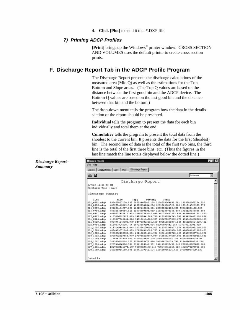
7-108 • Utilities 1/05
4. Click [Plot] to send it to a *.DXF file.
7) Printing ADCP Profiles [Print] brings up the Windows® printer window. CROSS SECTION AND VOLUMES uses the default printer to create cross section prints.
F. Discharge Report Tab in the ADCP Profile Program The Discharge Report presents the discharge calculations of the measured area (Mid Q) as well as the estimations for the Top, Bottom and Slope areas. (The Top Q values are based on the distance between the first good bin and the ADCP device. The Bottom Q values are based on the last good bin and the distance between that bin and the bottom.)
The drop-down menu tells the program how the data in the details section of the report should be presented.
Individual tells the program to present the data for each bin individually and total them at the end.
Cumulative tells the program to present the total data from the shoalest to the current bin. It presents the data for the first (shoalest) bin. The second line of data is the total of the first two bins, the third line is the total of the first three bins, etc. (Thus the figures in the last line match the line totals displayed below the dotted line.)
Discharge Report--Summary

1/05 Utilities • 7-109
Discharge Report--Details
XX. ADCP to DXF This program converts ADCP data to a DXF format file. Using the resulting files, you can: • Display current vectors as background files in HYPACK® MAX • Plot current vectors to smooth sheets in HYPLOT or HYPLOT
MAX. • Import them to other packages such as AutoCAD.
The process is very straightforward. 1. Select UTILITIES-ADCP-ADCP2DXF and make a selection
in each field. Most are self-explanatory.

7-110 • Utilities 1/05
ADCP to DXF dialog
Input ADCP Filename is the path and file of the ADCP data you wish to convert.
Output DXF Filename names the path and filename where the exported data will be saved.
Vector Type Flood Stream
Ebb Stream
Restricted Current
Vector Label Units: The current speed will be written above each vector in user-defined units. Select None to disable the labeling feature.
Attach Depth to Label includes the depth of the reading with the speed. The units will match the Distance and Depth Unit.
DXF Layer is the name of the layer in the output file where the data will be stored. It defaults to "ADCP Layer".
Distance Between Vectors prevents the vectors from overwriting and becoming, therefore, illegible in your DXF output file. The program includes only a selection of data points that are the specified distance (or more) from each other.
Current Depth Level enables you to specify the depth level you want to convert to the DXF file. • If the value is set to zero, the program will use the shoalest bin
from the ADCP records.

1/05 Utilities • 7-111
• If the value set is deeper than the ADCP measured current profile, no data will be converted.
2. Click [Convert] and the ADCP data will be saved to a DXF file in your project directory.
Resultant DXF Output
XXI. Hardlock Test A hardlock is required by HYPACK® MAX to activate the program modules associated with the license purchased. The HARDLOCK TEST program is used to check your HYPACK dongle type. The program searches for the different types of hardlocks distributed in the HYPACK's various software packages and displays your hardlock status.
A. Running the Hardlock Test To Run the test click on UTILITIES-OTHER-HARDLOCK TEST. A window will appear on your screen.

7-112 • Utilities 1/05
Hardlock dialog
The Hardlock Status includes the following: • All Hardlock Types detected will be checked under Hardlock
Keys. If no key is available, it will show Demo Mode. • User Name and ID Number • Date and Reseller Name • Key Number • ARCS User PIN which is used in a routine to enable you to use
ARCS background charts. • Copyright Date of the software.
B. Hardlock Problem Solving When you install HYPACK® MAX on Windows®2000, or WindowsXP, the hardlock driver will not install unless you are in Administrative Mode and have the Administrative Password.
While running the program, if you have a real Hypack® key and it keeps coming up in Demo Mode:
Hardware Try the key on a different computer. Remove other hardlocks to see if they are interfering with one another. Install a new parallel port on your desktop. Replace the hardlock. If you have a Glenco hardlock, it may be time to replace it with a newer one with wider compatibility and a special noise filter for "noisy" parallel ports. Your hardlock may also just be damaged in some way. We will replace it at a nominal fee (our cost + s&h). Try one of our USB keys (available after May 99) if you have a USB port. The key may simply need to be "ReBurned". It is now possible to get an internal key that occupies an internal ISA slot . We also have a key that works on a serial port

1/05 Utilities • 7-113
Operating System
Slow the computer's hardware key security check and direct its search locations by adding the following lines to the autoexec.bat: SET SSI_ACT=1000,1000,1000 SET HL_SEARCH=278i,378i,3bci Set your parallel port mode to Normal or Unidirectional in your system bios. In the NT Operating System, Windows®2000 or Windows®XP, you must be in "Administrative mode". They also require Remove Dr. Watson by deleting two files in the c:\winnt\system32 directory--drwatson.exe AND drwtsn32.exe. Defeat your power management settings. Make sure the parallel port is not “asleep”, as some notebooks do.
Software Certain programs lock up the hardlock checking process. Delete any HP Bi-directional printer drivers or HP monitoring programs and Turn off any screen savers. Format the hard drive and load WIN9x from a standard version. Certain companies (COMPAQ and TOSHIBA just to name 2) load a proprietary form version of Win9x as their operating system that interferes with the parallel port. If you are running Windows®NT 4.0 or Windows® 2000, look to see if Dr. Watson has been installed. If so, remove two files in the c:\winnt\system32 directory--drwatson.exe and drwtsn32.exe. They have been known to cause trouble in several programs including trouble with the hardlock key in Hypack®.
XXII. Seabed Statistics SEABED STATISTICS is the routine where you can define a set of classifications for your project area in a Seabed ID Square. The Seabed ID Square includes: • a list of bottom types • their corresponding E1 and E2 ranges from the echosounder
data. (You have to have a Seabed ID system.) • a seabed identification color and number for each bottom type.
All of the data is saved to your project in an *.SIX file.
The Seabed ID Square is used with the SeabedID device driver to apply classification numbers to each sounding record according to the E1-E2 range in which it falls. Once this is done, you can use the Seabed ID colors to display your soundings in HYPACK® MAX or plot your soundings and track lines in HYPLOT MAX. A TIN Model drawn with an XYZid file will draw to the screen using Seabed ID colors. You may also export your soundings in limited formats.

7-114 • Utilities 1/05
SEABED STATISTICS can also read All format data containing seabed ID information (the E1 and E2 data), and graph the distribution of each set of data. The graph also indicates the return ranges within which 68% and 95% of the returns fall.
A. Creating a Seabed Square in Seabed Statistics Before you can define the square, you must collect some sample data in various parts of your survey area where the bottom compositions differ to determine what bottom types exist and what their corresponding E1and E2 ranges are. The number of readings necessary will vary depending on how much your survey area varies.
If you are working in the same general area of the world where the geological conditions are similar, it may be possible to use the same square for several projects. However, if the bottom types are significantly different, you will have to create a seabed ID square appropriate to each project area. (You wouldn't use the same square file in the Mississippi delta as you would on the rocky coast of Maine.)
Once you have gathered this information, you are ready to build your Seabed ID Square. 1. Launch the SEABED STATISTICS by selecting UTILITIES-
OTHER-SEABED ID.
The Seabed ID window displays five resizable windows that can be toggled on and off through the View menu. Each will be described in the following sections. 2. Select FILE-NEW SEABED ID SQUARE. The screen will
clear, ready for the new information. 3. Load calibration data (optional). You can load your data files
or just representative "calibration points" from each bottom type area to guide you.
4. Define your bottom types with their corresponding E1 and E2 ranges. You can load your data files or just a representative "calibration point" from each bottom type area to guide you.
5. Modify the seabed identification colors (optional). SEABED STATISTICS automatically assigns colors to each color range, but you can change them by double clicking on the sample color to the left of each range description. A color dialog will appear for you to select your desired color.
6. Save the square by selecting FILE-SAVE SEABED ID SQUARE and naming the file. The file will be saved with a SIX extension in the project directory.
Note: You can choose to also save the same colors and ranges to the project's Hypack Color File (*HCF) which will allow you to display your data using your seabed identification colors.

1/05 Utilities • 7-115
1) Loading Calibration Data to Seabed Statistics You can enter your sample data files, or manually enter information derived from them, to be displayed in the Seabed ID Square window. This data is useful to guide you while you define your E1 and E2 ranges for each bottom type.
(a) Loading Data Files to Seabed Statistics To load the data files to SEABED STATISTICS select FILE-ADD MATERIAL then the Raw or All format files from the file selection dialog. When you do this the files are listed on the tree view file list at the left of the main window and displayed in the Seabed ID Square window.
Ideally, there would be one file for each bottom type. Whether you load them individually or using a LOG file, each file will display in a different color (up to 15) in the Seabed ID Square window.
Tree View File List
Viewing Sample Data
If some of your data files overlap, you can bring one set forward in the display by right clicking on the name in the tree view and selecting the "Highlight" option.
To unload data files from SEABED STATISTICS, right click on the name in the tree view and select the "Remove" option.
(b) Entering Field Samples to Seabed Statistics To enter a list of field samples, open the Calibration Points tab of Spreadsheet window and enter your bottom types with approximate E1 and E2 values. In this spreadsheet, the Notes field names the sample; it is not the seabed identification.

7-116 • Utilities 1/05
Entering Calibration Points
A blank Seabed ID Square with Calibration Points displayed
2) Entering Seabed Classification Ranges in Seabed Statistics You can do this using one or both of the following methods. • Manually type the information to the Limits tab of the
Spreadsheet window. d. Enter your list of E1 and E2 ranges that define each
bottom type. e. Provide a name for each bottom type .
As each classification is defined, the corresponding box will be drawn in the Seabed ID Square window.

1/05 Utilities • 7-117
The Edit Ranges Spreadsheet
The resulting Seabed ID Square
Range Edit Icon
• Use the cursor to draw the ranges in the Seabed ID Square window. Click the Range Edit icon, then use the cursor to drag a block around areas that define your classification ranges. The same cursor can be used to resize or relocate the blocks if necessary. The coinciding E1 and E2 ranges are automatically entered in the spreadsheet and an identification color is assigned.
B. Creating Seabed Statistics The second function of SEABED STATISTICS is to read and analyze the E1 and E2 values in the survey data you have loaded to the program, then present statistical information about it. Four windows display the data statistics.
When you load survey data to SEABED STATISTICS: • The file names are listed in the tree view on the left. • The statistics are automatically calculated and displayed.
Beware! If you have loaded data files that should not be included in the statistical analysis, you must omit them from your display and

7-118 • Utilities 1/05
statistical calculations by right clicking on the name in the tree view and clearing the "Enable" option.
▪ E1 Distribution and E2 Distribution windows: The distribution of the E1 and E2 values are graphed in the two distribution windows.
E1 Distribution Graph
E2 Distribution Graph
▪ The Material Statistics display presents the same data in
numeric form.
Material Statistics
▪ The Seabed ID Square overlays the E1 and E2 data on the
classification squares.

1/05 Utilities • 7-119
E1 and E2 overlays the Seabed ID Square
1) Editing E1 and E2 Data in Calculating Seabed Statistics The tools in the Seabed ID Square window enables you to remove any data from the statistical analysis. You can omit selected data points or entire files.
To omit select data points: 7. Click on the Material Selection Icon (right-most on the
toolbar). 8. Drag an area around the data you want to remove with your
cursor. The selected points will turn white. If you are not satisfied with the selection, you can: ▪ Make a new selection by dragging a new area. ▪ Deselect the data by selecting EDIT-CLEAR SELECTION.
9. Select EDIT-DELETE SELECTED MATERIALS or hit the Delete key. The Material Statistics and the E1 and E2 Distribution displays will all update accordingly.
To omit entire data files from your display and statistical calculations by right clicking on the name in the tree view and clearing the "Enable" option.
Note: This does not delete the data from the data files.
C. Reassigning Seabed Identification Values The Seabed Square is used by the SeabedID.dll to assign Seabed Identification values to each sounding record. In SEABED STATISTICS, you can reassign these values based on a different Seabed Square. When you do this, SEABED STATISTICS creates a new set of data files with the modified identification numbers. 1. Open the new Seabed Square by selecting FILE-OPEN
SEABED ID SQUARE. 2. Load your sounding files by selecting FILE-ADD MATERIAL
then the Raw or All format files from the file selection dialog.

7-120 • Utilities 1/05
3. Select FILE-REMAP MATERIAL. A dialog will appear with a number of options for naming the resulting new files.
Seabed Statistics Remap Dialog
Text Extension sets the extension to be used in naming the files. There are three ways this text can be used. The following table describes each option. The sample names result from using "new" as the text to reassign 041_322.edt which is listed in the FirstOne.log. • Add File Extension adds a "." followed by your text to the end
of your text name. Ex. 041_1322.edt.new, FirstOne.log.new.log • Change File Extension replaces the original extension with the
text. Ex. 041_1322.new, FirstOne.new.log • Add Text to Filename Beginning begins each file name with
your text. Ex. new041_1322.edt, newFirstOne.log.
D. Exporting Seabed Data to a Text File SEABED STATISTICS can reassign the seabed identification values and export user-selected data to a text file. 1. Load your seabed square. The identification numbers exported
will be based on this square. 2. Load your edited data files. The depths, E1 and E2 data will
come from these files. 3. Select FILE-EXPORT MATERIAL and the XYZ/ID Export
dialog will appear for you to choose your export options.
XYZ ID Export Dialog
Filename: Click the File Open icon and define the path and name for the exported file.

1/05 Utilities • 7-121
Fields To Export provides a series of check boxes, one for each type of data that may be included in the resulting text file. Check those that you wish to export along with the Delimiter that will separate each value. 4. Click [Export] and the text file will be created according to your
choices.
E. Converting Seabed Identification Colors to Project Colors You can export your Seabed Identification colors from SEABED STATISTICS to your project colors. By doing this: • SURVEY can color-code the matrix using Seabed ID colors. • HYPACK® MAX can display a seabed matrix using seabed
colors.
You can export your colors: • When you save your SIX file, SEABED STATISTICS asks you
if you would like to save the color codes to an HCF file (HYPACK® Color File) and transfer the seabed color coding to the project color settings. The new HCF file will be named SixFileName_SIX.HCF.
• Using FILE-EXPORT ID SQUARE TO HYPACK® COLOR FILE and naming the file.
In either case, the new HCF file will be saved to the project directory. When you exit SEABED STATISTICS, it will be implemented in the HYPACK® display.
In order to avoid confusion, a brief explanation about how this works with seabed identification data is in order.
Each cell in a matrix file actually has space in the matrix code for two depths. (This is what allows us to show the survey depth, dredge depth or the difference between the two values in dredge projects.) When you are collecting seabed identification data, the SeabedID device driver stores the seabed identification number in the first memory space, and the depth in the second.
The HCF file normally specifies the color that goes with each depth range. When SEABED STATISTICS exports the seabed colors to the HCF, it saves a range for each seabed identification number (plus and minus 0.5) with its corresponding color. Since the seabed identification numbers are stored in the first "depth" memory, SURVEY reads it as a depth and colors the matrix accordingly.
To display a seabed matrix using Seabed ID colors in HYPACK® MAX, right click on the Matrix folder in the Project Files list and select Seabed ID.

7-122 • Utilities 1/05
XXIII. Cross Check Statistics The STATISTICS program enables you to compute and display the sounding difference between intersecting survey lines. The program provides a statistical report showing the standard deviation distribution and average error. The output report contains detailed information for every intersecting point. • High Mean Difference, Low Std. Dev.: There may be a
systemic error that caused all of the check lines to be higher/lower than the normal lines.
• Low Mean Difference, High Std. Dev.: This means that you have an equal number of values in the check lines that are above and below the mean difference. They average out in the end, but there will be large differences in some intersections.
• High Mean Difference, High Std. Dev.: Time to stop the survey and figure out where you’re going wrong.
• Low Mean Difference, Low Std. Dev.: Optimal results. Good job!
A. Running the Statistics Program 1. Start the STATISTICS program by clicking UTILITIES-
OTHER-STATISTICS. 2. Open the Input dialog by selecting FILE-OPEN. The Input
dialog appears. 3. Fill the Input dialog and calculate the statistics. A graphical
view of your results will appear on your screen.
Note: The LOG files and the Output file must all reside in the same directory. 4. View a 3-D View. 5. Print the statistics graph by selecting PRINT-SCREEN. The
Windows® printer window appears for you to send it to the printer.
6. View the Statistics Report by selecting VIEW-REPORT. The text file will be opened in Notepad.
B. Calculating Cross Check Statistics The Input Info dialog requires one or two Catalog (*.log) files. The program runs faster if the section lines and cross lines are assigned to separate catalog files. Each file should be entered (with their path) in the corresponding field. (The program will work properly even if the places for section and cross lines are reversed.)
Note: At times, it may not be clear how to separate the lines. In this case, they may all be listed in one catalog file which is placed in the Section File field while the Cross Line File field is left empty. The program will proceed using only the lines in the Section File.
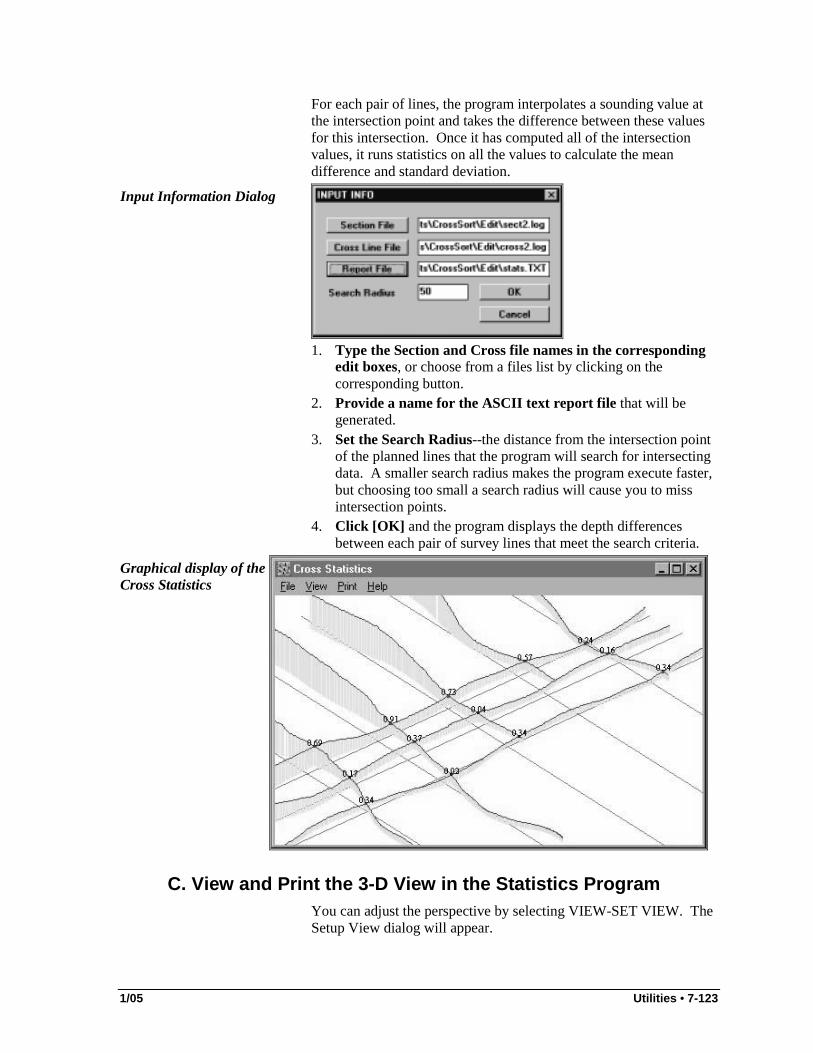
1/05 Utilities • 7-123
For each pair of lines, the program interpolates a sounding value at the intersection point and takes the difference between these values for this intersection. Once it has computed all of the intersection values, it runs statistics on all the values to calculate the mean difference and standard deviation.
Input Information Dialog
1. Type the Section and Cross file names in the corresponding
edit boxes, or choose from a files list by clicking on the corresponding button.
2. Provide a name for the ASCII text report file that will be generated.
3. Set the Search Radius--the distance from the intersection point of the planned lines that the program will search for intersecting data. A smaller search radius makes the program execute faster, but choosing too small a search radius will cause you to miss intersection points.
4. Click [OK] and the program displays the depth differences between each pair of survey lines that meet the search criteria.
Graphical display of the Cross Statistics
C. View and Print the 3-D View in the Statistics Program You can adjust the perspective by selecting VIEW-SET VIEW. The Setup View dialog will appear.
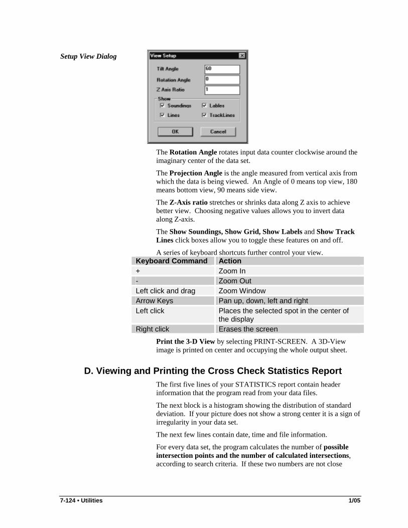
7-124 • Utilities 1/05
Setup View Dialog
The Rotation Angle rotates input data counter clockwise around the imaginary center of the data set.
The Projection Angle is the angle measured from vertical axis from which the data is being viewed. An Angle of 0 means top view, 180 means bottom view, 90 means side view.
The Z-Axis ratio stretches or shrinks data along Z axis to achieve better view. Choosing negative values allows you to invert data along Z-axis.
The Show Soundings, Show Grid, Show Labels and Show Track Lines click boxes allow you to toggle these features on and off.
A series of keyboard shortcuts further control your view. Keyboard Command Action + Zoom In - Zoom Out Left click and drag Zoom Window Arrow Keys Pan up, down, left and right Left click Places the selected spot in the center of
the display Right click Erases the screen
Print the 3-D View by selecting PRINT-SCREEN. A 3D-View image is printed on center and occupying the whole output sheet.
D. Viewing and Printing the Cross Check Statistics Report The first five lines of your STATISTICS report contain header information that the program read from your data files.
The next block is a histogram showing the distribution of standard deviation. If your picture does not show a strong center it is a sign of irregularity in your data set.
The next few lines contain date, time and file information.
For every data set, the program calculates the number of possible intersection points and the number of calculated intersections, according to search criteria. If these two numbers are not close

1/05 Utilities • 7-125
enough, it means that your search radius is too small, or your data set is incomplete.
Arithmetic Mean and Standard Deviation are calculated using well-known statistical formulas. The table at the end shows information about intersecting points which includes z1: height at row header file, z2: height at column header file, dif: z1-z2. If the intersection data is empty, n/a is displayed.
The Statistics Report
View your report by selecting VIEW-REPORT. The report is loaded into the Windows Notepad program, where it can be viewed or printed or both.
Print your report without previewing it by selecting PRINT-REPORT. It will be printed according to the print settings in Notepad.
Set Printer brings up the presents the standard Windows Printer Setup dialog. It was our intention that you could set up your print job from inside HYPACK® MAX. It was a good idea, but currently it does not work. Notepad overrides our settings. So…
To print your report: 1. Select VIEW-REPORT. This displays your report in Notepad. 2. Select FILE-PAGE SETUP and setup your print options. 3. Select FILE-PRINT to send the print job to the printer.
E. Example in Cross Check Statistics Example: Statistics Program Use the Sect.log and Cross.log in the Statistics project to run a
Statistics report.

7-126 • Utilities 1/05
1. Start the STATISTICS program by selecting UTILITIES-OTHER-STATISTICS. The Statistics dialog will appear.
2. Select FILE-OPEN to access the Input dialog. 3. Fill in the Input Dialog.
Input Information dialog
▪ Click on [Section File] and select the Sect.log from the Edit
directory of the Statistics project. ▪ Click on [Cross Line File] and select the Cross.log from the
same directory. ▪ Click [Report File] and name the text file where the statistics
will be saved. ▪ Enter your search radius and click [OK]. The statistics will
be calculated and saved to the text file as indicated. They will also be graphically displayed in the STATISTICS window.
4. Print the graph by selecting PRINT-SCREEN. The Windows® printer dialog will appear to set your printer options and send it to print.
5. View your report in text form by selecting VIEW-REPORT. The text file will be opened in Notepad.
6. Print this report by selecting FILE-PRINT in either Notepad or STATISTICS. The Windows® printer dialog will appear to set your printer options and send it to print. ▪ Positive differences show that Section File data is above
Cross Line File data. ▪ Negative differences show that Section File data is below
Cross Line File data.
XXIV. Channel Condition Reporter The USACE_RPT program is special utility developed for USACE-New England District, which automatically generates Channel Condition reports.
A. Channel Condition Reporter Interface Load the program by selecting UTILITIES-FILE WORK-OTHER-CHANNEL CONDITION REPORTER. The screen will contain a blank screen with a menu (top), the Object Editor (on the left) and a tool bar (on the right).

1/05 Utilities • 7-127
Channel Condition Reporter
The Tool bar assists you in navigating the screen when you have objects displayed.
The Measure Tool can be used to measure the distance and azimuth between two points in the area map. Just click the Measure Tool icon then click and drag between the two points on the map.
Unzoom can undo the last 20 zoom commands.
The cursor position and zoom ratio is displayed in the status bar.
The Object Editor lists all charts, reaches and basins that have been loaded to the project. Right click on any item to display a menu appropriate to it. Many of these options are also available through the menu.
B. Running Channel Condition Reporter Program 1. Start Channel Condition Reporter and open a project. Select
FILE-NEW for a new project. (Use FILE-OPEN PROJECT SETTINGS for existing projects.)
2. Create your Channels. 3. Set your Channel Properties. 4. Create your Reaches. 5. Save your Channel and Reach settings. 6. Load your Sounding Data. 7. Determine your Shoal Data. 8. Preview your results. 9. Generate your report.

7-128 • Utilities 1/05
1) Defining a Channel in Channel Condition Reporter 1. Load a DGN or DXF file into the project by selecting
DIALOGS-CHANNEL DEFINITION (or clicking [CHNL DEF]) and entering the name of your file. ▪ A closed polygon which represents the outer limits of your
channel ▪ A 3-D polyline which represents the centerline of your
channel
When you first load your background file to the screen, the program may do a poor job zooming on the contents. You can use the Zoom Window tool to click and drag around your area until it is an appropriate size.
Primary DGN Loaded to the Project
2. An additional background chart is an optional file that may
be loaded to enhance the on screen display. It does not affect the report. Select DIALOGS-BACKGROUND CHARTS and choose the file.
3. If are using a DGN file for your Channel Definition file, select the layers for display. Select DIALOG-DGN LAYER DISPLAY and a dialog will appear listing the layers in the chart. Check the boxes for any layer you wish to include. (Right click in the list area and use the pop-up menu selections to check All or None of the boxes.) [Apply] lets you preview the results of your selections in the map view.
Note: This feature is not available for DXF files; it's all or nothing for them.

1/05 Utilities • 7-129
DGN Layer Control Dialog
4. Assign Limits to the centerline, and inside and outside lines on
each side of center. a. Select TOOLS-ASSIGN LIMITS or the Assign Limits icon
and a dialog will appear.
Assign Limits Dialog
b. Choose the Channel Type.
! Single Channel generates a report of information across the entire channel.
! Quarter Half Quarter divides the channel longitudinally into 3 divisions (outside left quarter, inside half, outside right quarter) and presents the data by division.
! Four Quarter does the same with four divisions. c. Define your channel.
i. Select "Channel Limits" . ii. One at a time, select one of the lines in the dialog to
be defined, then click on the corresponding line in the map. The selected line will change color until you select another line in the dialog.
Note: To determine the left and right sides of the channel, imagine that you are standing at the beginning of the centerline looking down the channel. Be sure these are defined accurately. If you are unsure,

7-130 • Utilities 1/05
take your best guess, then create your reaches. The first reach divider will appear at the beginning of the centerline. If you assigned the limits incorrectly, start over and reverse your lefts and rights.
It may be easier to accurately select the lines in the map if you have turned off the display of other layers, even if only temporarily, in the Layer Control dialog.
d. If your channel includes a turning basin, select "Turning Basin" then click on the basin line on the chart. The Basin Editor will appear. Enter your settings and click [OK].
Basin Editor
The Basin Name is used in the Object Editor's file list.
You can check "Override" and set a Basin Depth different than the Channel Depth.
The Gutter creates lines at a user-specified distance inside the basin perimeter. If a gutter is created, the report generated will exclude the data in these zones from the available depths for the channel. The shoalest depths will be footnoted in the report, but they will not be recognized as controlling depths. Excluding the distance along the shore acknowledges and defines sloping banks, and focuses the report on the center navigable area.
Note: At a later time, you can access this dialog to modify these settings by right clicking the Basin Name in the Object Editor and selecting "Properties". 5. Create the Channel. When all of the lines have been assigned,
click on [Close] to exit the dialog and store the information.
2) Setting your Channel Properties in Channel Condition Reporter
Enter the Channel Properties by selecting CHANNEL-PROPERTIES or clicking [Channel]. The Channel Properties dialog will appear.

1/05 Utilities • 7-131
Channel Properties Dialog
The Channel Name can be any name you choose with 2 lines available.
Producer Name and Address is included in the header of the final report.
The Survey Date represents the day(s) when you conducted the survey upon which the report is based.
The Project Depth is assigned to the entire channel. You can "over-ride" this value for an individual reach by right clicking on the Reach name on the map and selecting PROPERTIES. A dialog will be displayed in which you may edit the settings for that reach.
Footnote Configuration: Footnotes list soundings excluded from the available depths for the channel by any Outer Left and Outer Right Distances set in the Reach Properties. (See "Setting Reach Properties in Channel Condition Reporter") The minimum footnote includes the excluded depth and its distance from the left or right channel limit. You can choose to also include the sounding's lat./lon. position in either WGS84 or using local grid coordinates presented in your choice of three Lat./Lon. Formats.
The Shoal Color displays the current color for the shoal soundings display. Click [Shoal Color…] to set a different color.
3) Creating your Reaches in Channel Condition Reporter You can divide the channel into any number of reaches. Each reach will be presented with a separate set of statistics in the Channel Conditions Report. 1. Select DIALOGS-MULTIPLE REACHES (or click
[Reaches]) and a dialog will appear.

7-132 • Utilities 1/05
2. Define either the number of reaches you want, or the distance a reach covers. Click [OK] and dividers will be drawn across the channel accordingly.
Reaches displayed along the channel
The properties of each reach will default to the channel property settings, but they may be edited through the Reach Editor described in the "Setting Reach Properties" section.
Insert additional dividers by selecting the Reach Tool and clicking at the position in the channel where you want the new divider.
Delete a divider by right clicking on the handle of the divider and selecting Delete Divider.
Reposition a divider by clicking and dragging the handle in the center of the divider.
4) Setting Reach Properties in Channel Condition Reporter Right click on a reach handle (or on the reach title in the list on the left) and select "Properties". The Reach Editor will appear.
Reach Editor
Reach ID specifies which divider is described. You can change the name if you wish.

1/05 Utilities • 7-133
Reach Depth displays the channel depth from that divider to the next. Check Override to enable a change in the depth for that segment only and type in the new depth.
Reach Width and Length are displayed, but may not be edited.
Orientation offers 3 choices: • Minimum Distance positions the divider at the angle where it
crosses the shortest distance between the outside left and right lines of the channel.
• Perpendicular positions the divider perpendicular to the outside lines.
• Set Angle enables you to set the angle at which the divider crosses the channel.
Note: The divider must cross the outer left and right sides. If the orientation entered does not allow this, the divider orientation will not change.
OLT (Outer Left) and ORT (Outer Right) Distances may be specified for each reach. This option creates longitudinal lines at the specified distances, parallel to the left and right toe lines respectively. If these are created, the report generated will exclude the data in these zones from the available depths for the channel. The shoalest depth in these zones, if less than project depth, will be footnoted in your final report. (They will be totally excluded from the Segment Review.) Excluding the distance along the shore acknowledges and defines sloping banks, and focuses the report on the center navigable area.
5) Saving Your Channel and Reach Settings in Channel Condition Reporter
Save your Settings by selecting FILE-SAVE PROJECT or FILE-SAVE PROJECT AS and naming your file. The information you have set so far will be saved with an .RPT extension. For future reports for this same channel, you can save time by selecting FILE-OPEN PROJECT and select the RPT file to get to this point in the process.
6) Loading Your Soundings Data in Channel Condition Reporter Load your Soundings data file. Select DIALOGS-LOAD SOUNDINGS (or click [XYZ], select Load Soundings) and select your file. The CHANNEL CONDITIONS program supports the use of either a HYPACK® XYZ file or a DGN file. Typically, this file will be a sorted HYPACK® File. All of the soundings in the file will be drawn to the screen without regard to overwrites.
Note: Soundings are not saved when you exit CHANNEL CONDITIONS REPORTER. Even if the project settings are saved, the soundings must be reloaded each time you re-open the project in the program.

7-134 • Utilities 1/05
Soundings Loaded to the project
(a) Sounding Display Settings Display settings are defined in the Sounding Display dialog. Select DIALOGS-SOUNDINGS-SOUNDING DISPLAY (or click [XYZ] and select Sounding Display) and the Sounding Display dialog will appear.
Sounding Display Dialog
If you wish to omit larger soundings, check the box and specify the depth limit. Soundings larger than this value will not be displayed.
Change sounding colors by clicking [Color Table] and defining the range, increment and color scheme as described for HYPACK® MAX in Chapter 1. [Apply] allows you to preview the effect of your changes on the sounding display before leaving the dialog. Color changes made here will remain in effect for your project when you close the CHANNEL CONDITION REPORTER.
If you have loaded soundings in DGN format, define for CHANNEL CONDITION REPORTER which layer of your DGN file to display by entering it under DGN Layer to Extract Soundings.
Note: Though the Sounding files must always be reloaded when you re-enter a project in this program, the display settings from the Sounding Display Options dialog are saved with the project settings.

1/05 Utilities • 7-135
If changes are made in the sounding display options, you should save the project settings before exiting the program.
(b) Inverting Depths If your file is XY(-Z), invert the depths. 1. Load the soundings file. 2. Double click on the "Charts" item in the Object Editor to expand
the tree view. 3. Right click on the name of the XYZ file. 4. Click "Invert Depths" to negate all to the depths.
7) Determining your Shoal Data in Channel Condition Reporter Click on [Shoals]. The program will go through the Soundings file and determine the minimum depth in each reach and any other shoals that are less than the project depth as specified in the Properties window.
On the screen display you’ll see different colored depths. • Red = Controlling Depth • Yellow = Shoals, deeper than the Controlling Depth, but shoaler
than Project Depth. You can choose another in the Channel Properties dialog.
• Blue = Would have been a Controlling Depth, but it lies in an OLT or ORT zone.
Shoals Display
8) Previewing your Results in Channel Condition Reporter Preview your report by segments (optional). The results may be viewed, one reach at a time, by clicking [Review]. The Segment Review dialog appears. Select the Reach and, unless you have chosen the single Channel Type, the segment you want. The description, controlling shoal and additional shoals in the defined area will be displayed.
Export your Shoal Depths or your Controlling Depths (or both) to an XYZ format file. Just check the corresponding box or boxes and click [XYZ Output]. Name the output file in the dialog

7-136 • Utilities 1/05
presented and it will be saved by default to the Sort directory of your project. You can view these depths later in the main window by enabling the output file in the Sorted files list.
Since the XYZ output file does not distinguish between the Controlling Depths and the Shoal Depths, you may wish to export one set of depths at a time so they may be loaded separately for viewing in the main window.
Segment Review Dialog
9) Generating your Reports in Channel Condition Reporter Generate your report by clicking [Report] and selecting "screen" or "text file". This option generates the ER-1130-2-416 Channel Condition Report. Most is self-explanatory. The Depths Available represent the controlling depths of each channel segment.
Note: Any Controlling Depths greater than the Project Depth will be reported as the Project Depth.
You may edit any field in the report. The rows may be adjusted in the spreadsheet using the corresponding buttons. [Printer] and [Font], display Windows® Font and Print dialogs to perform each of those functions.

1/05 Utilities • 7-137
A Sample Report Printed to the Screen
If you have MicroSoft Excel installed on your computer, you can export this report to an Excel spreadsheet by clicking [Export Xcel]. The Channel Condition Reporter will launch a copy of Excel and export the report data directly into a new worksheet.
XXV. 3D Terrain Viewer The 3D Terrain Viewer program (also known as 3DTV) is a versatile tool that enables you to closely examine a three-dimensional model of your survey or dredge data. 3DTV can be launched from the HYPACK® MAX Utilities menu to view existing data of your project area. You can also launch it from SURVEY or DREDGEPACK with existing data and view data updates in real time.
In Matrix 3DTV mode, your dredge operator can see a 3-dimensional representation of the dredge area and the changing contours of the area as material is removed from the area or your survey operator can see the terrain model created as the survey progresses.
Imagine that there is a camera flying above your project area sending the image to your computer and you are at the controls. You can direct the camera's flight to view the model from any angle except beneath it. Just load an XYZ data file or a Matrix file, and perhaps define a few settings and you're ready to go.

7-138 • Utilities 1/05
3DTV Interface
While you are viewing the data, you can use the movie tools to create a file that can later replay what you saw. In this way you can record the "points of interest" (or the entire survey) and review them at any time.
A. Running the 3DTV Program 3DTV can be run in two modes:
3DTV mode is launched from the main HYPACK® MAX window or from SURVEY or DREDGEPACK® to view existing data. The 3D Terrain Viewer mode is displayed in the title bar.
Matrix 3DTV mode is launched from SURVEY or DREDGEPACK to see a matrix (filled or empty) updated in real time. The Matrix 3DTV mode is displayed in the title bar. The file name is read from shared memory. 1. Launch 3DTV:
▪ In 3DTV Mode: ! from the main menu by selecting UTILITIES-OTHER-
3DTV or
! from the SURVEY or DREDGEPACK menu by selecting OPTIONS-SHARED MEMORY-3DTV.
The 3DTV interface will appear. The first time that you run the program in a project, the program will ask you to define a data set in an XYZ or MTX format and your choices for creating the model. Otherwise, it will load the data set and other 3DTV settings that have been most recently used in the project.
To open a different data set, select FILE-NEW then choose the new XYZ or MTX data file and define your terrain model settings.

1/05 Utilities • 7-139
▪ In Matrix 3DTV Mode from the SURVEY or DREDGEPACK® menu by selecting OPTIONS-SHARED MEMORY-MATRIX 3DTV. Since the purpose of Matrix 3DTV mode is to update depth data in an existing matrix with current depth data or to fill depth data in an empty matrix, Matrix 3DTV mode requires a filled (or empty). Matrix 3DTV Mode requires a matrix file to be enabled in your project. The program will always load the enabled matrix file.
The first time Matrix 3DTV is started in a project, it will ask for your terrain setting choices for creating the model. Otherwise, it will load the data set and other 3DTV settings that have been most recently used in the project.
2. Size your windows (optional). A new file will begin with default settings for your window sizing and position, visible toolbars, etc. A saved file will open with the settings that were active when it was last saved. If you prefer a different arrangement, reposition and resize the windows to suit you and use the View menu to turn toolbars and the status bar on and off. If you want this arrangement to be the default, select FILE-SAVE DEFAULT.
3. Select the flight mode in which you want to use 3DTV. Function Mode To manipulate the camera manually
Manual Flight mode
To simulate the view as you follow planned survey lines
LNW File mode
To follow the vessel trajectory supplied by the SURVEY program
SURVEY Program mode
To define and follow a circular path
Circle Flight
In Matrix 3DTV mode, only Manual Flight and SURVEY Program modes are available. 4. Set your display options. These include such things as your
display method, and color and lighting settings. 5. Use the camera controls to set your view angles and move it
across the project area. 6. Use the movie tools to make a record of what you see
(Optional). This is not recording survey data. It creates a specialized file that can replay your view in 3DTV, but does not contain your survey data. This file is saved to your project directory with a 3DM extension and can be used only for the purpose of replaying your movie in the 3DTV program. Alternatively, you can record it to an AVI file and replay it in a media player.
7. Save your current settings by selecting FILE-SAVE and providing a name. By default, 3DTV will save 3DTV mode information to the 3DV file in your project directory. The most

7-140 • Utilities 1/05
recently used settings will be used the next time 3DTV or Matrix 3DTV is launched from the same HYPACK® project.
To save the 3DTV settings in an alternate *.3DV file, select FILE-SAVE AS and name the file. This can provide you with a choice of settings so you can instantly change the objects, colors, and a number of other parameters in your display.
To load alternate project settings, select FILE-OPEN and select your alternate *.3DV file.
B. Terrain Settings in 3DTV When you are creating a new viewing, the 3D TERRAIN VIEWER will display the Terrain Settings dialog. (The same dialog can be opened by selecting TERRAIN-TERRAIN SETTINGS.) The options in this dialog affect how your model will be created in your Terrain Windows.
Terrain Settings Dialog
The Grid Cell Size defines width and height of the grid cell. The grid is used to detect camera-terrain collision conditions conditions in both 3DTV and Matrix 3DTV modes and to affect change in the drawing rate and quality of the model in 3DTV mode only.
The Grid Extents are derived by the program from the data set and are for display purposes only.
Max Edge Size is only required in 3DTV mode. It defines the longest distance between two horizontal plane projections of soundings that will be connected in the model.

1/05 Utilities • 7-141
Max Edge Size
You should set this large enough so your data points connect, but not so large that points which have little relationship connect to each other.
Z-Interpretation: If this option is enabled, choose whether your soundings should be interpreted as depths or elevations. Keep in mind that 3D Terrain Viewer always presents elevations (i.e. all displayed Z values in the program correspond to Z-axis directed upward).
The scale of the Z-axis of your terrain, as well as other objects displayed in your terrain window, can be adjusted using the vertical exaggeration feature. (See "Vertical Exaggeration" under "Display Options" for further discussion.)
Model: Logically, larger data sets tend to slow the frame rate in the Terrain window. You can trade some of the quality of the model drawn for a faster drawing speed by selecting appropriate model for your project. Experiment with these settings to see what works best with your computer and project needs.
The Static model does not change when camera moves. The model may be: • Accurate, based on points from the imported file. This option
draws the same type of detailed model that you may have seen in the TIN Model program—a Triangular Irregular Network
• Fast, that simplifies the terrain by drawing only one (center) point for each defined grid cell. This option creates the model based on the grid defined in the dialog—a TRN model (Triangular Regular Network) rather than a TIN model.
Note: When a matrix file is loaded in 3DTV mode and the Accurate option is selected, the model looks like a TRN structure, although it is actually a TIN structure.
The Dynamic model is reconfigurable during camera motion. It always presents terrain areas closer to the camera in greater detail.

7-142 • Utilities 1/05
When the camera moves, the terrain model changes to keep the refresh rate approximately constant.
When Dynamic mode is selected, you can further affect the speed and quality of your drawing by using the Quality/Speed slider. • Quality position will result in maximum level of model details
presentation. • Speed position will minimize the level of details producing very
rough images of the presented area and accordingly high frame rate.
The following figures demonstrate the differences. They are most evident in the wire frame models.
Static Accurate Presentation
Static Fast Presentation
Dynamic Quality Presentation

1/05 Utilities • 7-143
Dynamic Speed Presentation
• In 3DTV Mode:
When Static Fast mode is selected, you can further affect the speed and quality of your drawing by adjusting the cell size. Larger cell dimensions generate less-detailed models, which can be drawn even more quickly by 3DTV.
Note: Conversely, you can negate the effect of the Fast option by setting a small cell size.
All options mentioned above are available in the 3DTV program mode. • In Matrix 3DTV Mode:
The model is always drawn based on the cell size of the matrix that is currently loaded to SURVEY or DREDGEPACK. This means that the Cell Size in the Terrain Settings will have no effect on the model quality or drawing speed.
For the same reason, there is no difference between Static Accurate and Static Fast models in Matrix 3DTV mode. Therefore, the radio buttons Accurate and Fast will be disabled.
C. 3D Terrain Viewer Flight Modes The 3D Terrain Viewer can be run in four different modes. The mode is set by selecting CAMERA-FLIGHT MODE and your selection.
1) Manual Mode Manual Mode gives you full control to use the camera controls to view your data from almost any angle.
Camera Controls-Manual Mode

7-144 • Utilities 1/05
2) LNW File Mode LNW File Mode asks you to load a Planned Line (LNW) file and automatically simulates travel down each survey line in the file. Since this mode follows the survey line, the Turn controls are disabled, while orientation controls (Yaw and Tilt) are enabled. This option is only available in 3DTV mode.
In this mode, additional options appear in the camera controls. • The selected Planned Line file is displayed with a [Browse] so
you can load a different line file. • If the opened LNW file contains multiple lines, a control for line
number selection will appear. Select the line number and the camera will be positioned at the start point of the line and directed by the first segment of the line.
Camera Controls- LNW File Mode
• Camera Yaw, the angle relative to the line segment (path), will
default to 0 degrees. At this setting, the program will automatically change the camera heading for each new line segment to follow the changed direction of the survey line. The camera yaw will remain the same relative to the line path. when the line direction changes.
3) Survey Mode Survey Mode is used simultaneously with SURVEY (or DREDGEPACK®). In 3DTV mode, it might be useful to review previously existing data as you tour the survey area, while in Matrix 3DTV mode, you can watch the previous data being updated in real time as you survey. • If the vessel is not shown (VESSEL-SHOW is not selected), the
camera position and direction are taken from the Shared Memory created by the SURVEY program. It appears directly above the boat position and a Yaw setting of zero orients the camera to match the boat heading. Speed and Turn controls are disabled for this option as they are controlled by SURVEY. Camera orientation (Yaw and Tilt), zoom, and elevation change controls are enabled.
• If the vessel is shown, the camera is positioned relative to the vessel. (See "Vessel Display Options".)

1/05 Utilities • 7-145
4) Circle Mode Circle Mode automatically creates a circular path sized to fit your loaded data set. The camera travels clockwise around the path at a speed set with the speed controls. Its yaw and tilt are fixed to point toward the center of the circle and slightly downward. This enables you to view your model or an object in the model from all sides (as if you were walking around it). This option is only available in 3DTV mode.
Circle Mode—the camera travels clockwise around a circular path.
You can create a new path in the Camera Position Window. Just click where you want the center of the circle to be and drag a distance equaling the radius. Dotted lines will show the size and location of your new path until you release the mouse button and the path is created with the camera set at the point of release. When a new path is created, the speed will be reset to zero. If you are not happy with the results, try again.
D. Display Options in the 3D Terrain Viewer The 3D Terrain Viewer has several options affecting how you view your data. From within 3DTV, you can control the type of model created, the color scheme and lighting. You can also adjust the settings for the speed that the program can redraw the data in a window that has been repositioned.
Note: The settings are applied to the active 3D Terrain Window, and that you can select different display modes for different 3D Terrain Windows.
1) 3D Terrain Viewer Model Types 3DTV provides a choice to view your data as a solid, color-coded model or a white wire frame model. Select VIEW-DISPLAY MODE and make your choice.

7-146 • Utilities 1/05
Solid Model
Wire Frame Model
2) 3D Terrain Viewer Color Settings In each project, the first time 3D Terrain Viewer is opened from HYPACK® MAX, it will begin with the HYPACK® MAX color scheme.
To customize your color settings: 1. Select TERRAIN-COLOR SCALE-CUSTOM COLORS. 2. Select TERRAIN-COLOR SCALE-EDIT COLORS. This
displays the standard HYPACK® colors dialog for you to set your new color scheme.
Note: The custom colors only affect 3DTV. They are saved in the 3DTV project settings (and are restored when you later re-open the project *.3DV file), but they do not affect the project color settings outside of the 3DTV module.
To create multiple sets of custom colors for the same project, follow this procedure and save them to different 3DV files. If your desired settings are not in the most recently used project file (3DTV_Project.3DV for 3DTV or DV_Project.3DV for MATRIX 3DTV, which will be read when the program starts, use OPEN-FILE to select the appropriate 3DV file.

1/05 Utilities • 7-147
You can toggle between HYPACK® and Custom Colors by changing your TERRAIN-COLOR SCALE menu selection at any time.
3) Dynamic Lighting in 3DTV The dynamic lighting settings adjust the lighting in the 3D Terrain Viewer. Select LIGHTING-ENABLE to toggle this feature on and off.
To select your dynamic lighting settings, select LIGHTING-SETTINGS and the Dynamic Lighting Settings dialog will appear.
Dynamic Lighting Settings Dialog
Ambient light comes from "everywhere".
Diffuse light originates from the light source, which is precisely positioned in space.
To customize the color of each type of light click the corresponding button and select your color from the color selection dialog that appears.
Note: You are free to select any color. However, keep in mind that only the white light (or shades of gray, which represent the white light of lower intensity) would not affect colors of the solid model.
The Maximum Displayed Height is the vertical extent of the side view of the Light Position Window. It can be set • At a user-defined constant by entering a height value here. This
value may not be less than the default value which is calculated based on the current dataset. (Click [Default] to find out what that value is.)
.Note: The Maximum Displayed Height setting does not limit the height of the lighting source, but if the lamp height exceeds the user-defined height, it will not be visible in the Light Position Window. • Automatically by the program. The Automatic Adjust option
adjusts the Maximum Displayed Height based on the current light position. If your light position is near the top of the current range, the Maximum Displayed Height will increase; if the light is near the lower end of the range, the Maximum Displayed Height will decrease.

7-148 • Utilities 1/05
You can position the light source in Light Position Window. (If the Light Position Window is not visible, select LIGHTING-POSITION WINDOW.)
Light Position Window
There is one light source available for each incident of the 3D Terrain Window. The light settings are independent in each window. Changes made in the Light Position Window will be applied to the currently selected 3D Terrain Window. Both solid and wire-frame models are affected by the dynamic lighting.
Adjust the horizontal position of the light source on the left side of the window where an outline of your data file and a yellow circle that represents the light source are displayed. Click where you want your light source relative to your data and the circle will move to that location. The effect will be seen in the 3D Terrain window.
Adjust the vertical position of the light source on the right side of the window where the minimum and maximum Z-values of your data file are displayed. Click in that window at the height relative to the data where you want the light. The yellow circle will move to that location and the effect will be seen in the 3D Terrain window.
Synchronize the light position with the camera position using the Mining Lamp feature. Select LIGHTING-MINING LAMP (or enable the Mining Lamp Mode icon.) When the feature is selected, you can not adjust the light position manually.
4) Vertical Exaggeration The scale of the Z-axis of your terrain, as well as other objects displayed in your Terrain Window, can be adjusted using the Vertical Exaggeration feature. This can be particularly helpful if your terrain is nearly flat. Multiplying the Z-value by a factor larger than 1 accentuates even small changes in depth/elevation to optimize the viewing of your terrain. (You can also decrease the vertical change by entering a factor between 0 and 1.)
The water level, as well as the channel, and vessel will also be scaled by the same factor in order to keep the scale of the entire display synchronized.
Select VIEW-VERTICAL EXAGGERATION and enter a Z-scale factor in the Vertical Exaggeration dialog.

1/05 Utilities • 7-149
Vertical Exaggeration Dialog
Scale Factor=1
Scale Factor=5
5) Viewing a Water Surface in 3DTV You can improve the realism of the display by superimposing a water surface in your survey area. To do this, select OBJECTS-WATER SURFACE and check Enable.
Survey Data displayed in 3DTV-- No Water Surface(left)
Water Surface Enabled (right)
The Water Surface Level is also drawn in the Camera and Light Position Windows. In the following figures, the water level is represented by the line in the selected water color on the right side of the window.

7-150 • Utilities 1/05
The Water Level is drawn in the Camera and Light Position Windows
The water's level, transparency and color are controlled through the Water Surface Settings dialog. Select OBJECTS-WATER SURFACE-SETTINGS and the dialog will appear.
Water Surface Settings: Default Settings
The Chart Datum Level is the height of the chart datum above Mean Sea Level. It is read from your geodesy settings.
Note: If the control is enabled, the geodesy settings do not contain the value, so set it to the desired level. This Z value will be interpreted as elevation, regardless of Z-interpretation mode, since all displayed Z-values in the 3DV are elevations.
The Water Surface Level is determined by the Chart Datum Level and, in Survey Program Flight Mode, the Tide Correction value which is read from shared memory.
Transparency affects the transparency of the water surface. A value of zero results in an opaque surface while 100 causes it to become invisible.
[Color] displays a color dialog from which you can choose a color for the water in your display. Note that, unless you choose white, the color of the water will affect the color display of the depths below water level.
[Apply] updates the 3DTV window according to your settings without leaving the settings dialog.
[Default] resets the values to CDL = the value defined in the geodesy settings (or 0.0), Transparency = 80 and the Color to blue.
6) Viewing Planned Lines and Channel Information in 3DTV You can use the OBJECTS-CHANNEL menu to import and display planned lines and channel information in your 3D Terrain Window. Such information provides the dredger with important information to guide his navigation and improve digging accuracy.

1/05 Utilities • 7-151
The channel file can contain either depth or elevation data. The information on the expected Z-interpretation of channel file data will be read directly from the channel file or, if the mode is not indicated there, the mode will be set to match the Z-interpretation selection in the program.
(a) Importing Planned Lines and Channel Information to 3DTV
Load your choice of files by selecting OBJECTS-CHANNEL-IMPORT and the file type you want to view, then choose your file from the file selection dialog that appears. 3DTV accepts:
Feature Source Channel CHN files are Channel Plan files created in
ADVANCED CHANNEL DESIGN. Channel Lines
PLN files are Channel Plan files created in CHANNEL DESIGN. They include Toe Lines, Center Lines and Basin Lines.
Planned Lines
LNW files are created primarily in the LINE EDITOR or in CHANNEL DESIGN.
Planned lines will be displayed with their line name above each end.
Note: If you want to display channel lines with the planned lines, you would typically create the LNW file and PLN files both at the same time in CHANNEL DESIGN.
(b) Display Options for Planned Lines and Channel Information in 3DTV
Once you have loaded your choice of features, you can customize how they are displayed through the Channel Settings dialog which can be accessed by selecting OBJECTS-CHANNEL-SETTINGS. Take a little time to experiment with the different settings and you will quickly understand how they work and develop preferences for your purposes.
Channel Settings Dialog
For each type of feature, you can customize:
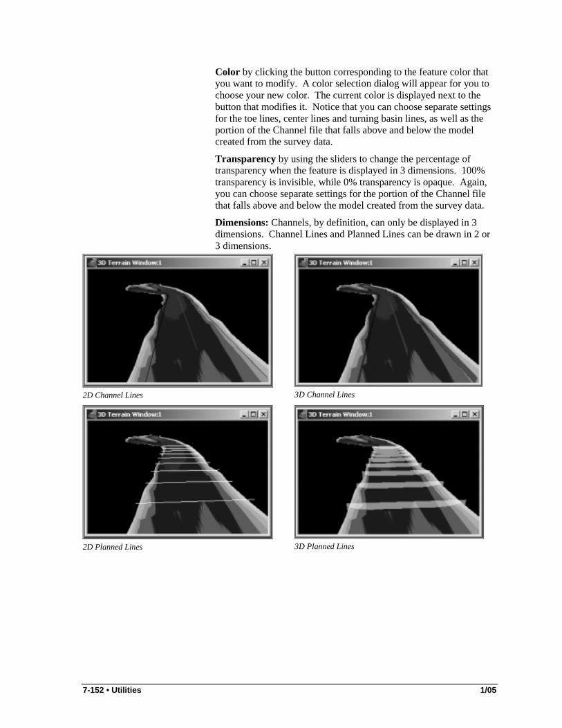
7-152 • Utilities 1/05
Color by clicking the button corresponding to the feature color that you want to modify. A color selection dialog will appear for you to choose your new color. The current color is displayed next to the button that modifies it. Notice that you can choose separate settings for the toe lines, center lines and turning basin lines, as well as the portion of the Channel file that falls above and below the model created from the survey data.
Transparency by using the sliders to change the percentage of transparency when the feature is displayed in 3 dimensions. 100% transparency is invisible, while 0% transparency is opaque. Again, you can choose separate settings for the portion of the Channel file that falls above and below the model created from the survey data.
Dimensions: Channels, by definition, can only be displayed in 3 dimensions. Channel Lines and Planned Lines can be drawn in 2 or 3 dimensions.
2D Channel Lines
3D Channel Lines
2D Planned Lines
3D Planned Lines

1/05 Utilities • 7-153
Channel Display
All Feature Types: 2D Channel Lines, 3D Planned Lines and Channel
Clip Against Terrain Extents: The ends of planned and channel lines will follow the boundaries of the ensonified area.
Note: The accuracy of the clipping is, affected by the Grid Cell Size set in your terrain settings. A smaller Grid Cell Size will clip the lines more closely to the edges of the ensonified area.
[Default] resets all settings to their defaults as shown in the sample dialog. All transparency settings are set to 50%, Channel Lines and Planned Lines are set to draw in 2 dimensions and each feature has a separate and distinct color.
7) Viewing Boat Shapes in 3D Terrain Viewer In Survey Mode, you can load a vessel shape that will be displayed in 3DTV according to the information received through shared memory. 3DTV uses information from shared memory to calculate the exact XYZ position of the vessel. Its origin (determined when the boat shape is created) is located at the current X,Y position. The vertical position of the vessel is adjusted according to the current chart datum level (CDL), and the tide and draft correction values. The vessel heading will coincide with heading data in shared memory.
If you show display a vessel, the camera will be positioned relative to the vessel according to the settings in the Vessel Settings dialog.
If no boat is shown, the camera is positioned at the boat position according to the information from shared memory.
(a) Loading Vessel Shapes There are 2 options if you want to include a boat in your Terrain Viewer display. You can: • Create a scale model of your survey boat or dredge (a custom
3D boat shape) in the 3D SHAPE EDITOR that can then be imported into 3DTV. (Details on this may be found under "3D Shape Editor".) or

7-154 • Utilities 1/05
• Load the 3DTV default boat shape to represent your vessel.
To load your custom 3D Boat Shape: 1. Select VESSEL-IMPORT VESSEL. A File Select dialog will
appear. 2. Select the appropriate VES file and click [OK]. 3. Select VESSEL-SHOW.
Importing a Custom Boat Shape to Matrix 3DTV
3DTV includes a default boat shape that is only a "generic" representation to mark your vessel position on the screen. It's quick and easy if an accurate representation of your vessel is unimportant to you.
To load 3DTV's generic boat shape: 1. Select VESSEL-DEFAULT SHAPE. 2. Select VESSEL-SHOW to toggle the display of the vessel in the
3D Terrain window.
Importing the Default Boat Shape to 3D Terrain Viewer
(b) Vessel Display Options Once the boat is loaded and showing, you can view your data and your vessel as the survey progresses. You can also elect to include the vessel's shadow.

1/05 Utilities • 7-155
The Vessel Settings dialog provides display options that affect your view of the boat.
Select VESSELS-SETTINGS to access the Vessel Settings dialog.
Vessel Settings Dialog—
Defaults are shown.
Camera Position Relative to Vessel: When a vessel is showing, the camera is positioned relative to the boat rather than at the boat position. The Camera Position settings enable you to set the angle and distance from the boat where the camera should be located. As the vessel moves, the camera position will update to maintain these distances. • Behind (default=50) positions the camera to follow the vessel by
the defined distance. A negative value positions the camera in front of the vessel. (In this case, you probably want to check the Focus the Vessel option so the camera will face the vessel and move backward.)
• Aside (default=0) offsets the camera port or starboard of the vessel midline. A positive distance value positions the camera to the port side, while a negative value moves the camera starboard.
• Above (default=18.2) places the camera above the vessel reference point by the specified distance. You can use a negative value to view the vessel from beneath the waterline, but you can not position the camera below the survey bottom.
Focus the Vessel keeps the camera facing the boat regardless of where it is positioned. If this option is cleared, you can manually focus the vessel using the Focus on Vessel icon on the tool bar.
[Vessel Color] displays a color dialog from which you can choose a color for the default vessel.
Scaling Factor increases and decreases the size of the vessel display. It affects either the default or a custom boat shape.
[Apply] updates the vessel settings allowing you to preview your display without leaving the settings dialog
[Default] sets all of the settings to their default value. These values are shown in the previous figure.

7-156 • Utilities 1/05
In addition to the options in the Vessel Settings dialog, the Vessels menu includes a number of features that can be toggled on and off.
Show Shadow: If a boat shape is showing, you can also display the shadow of the shape on the survey bottom, positioned directly below the boat (regardless of the light source position). It may be very useful to know exactly where you are above the terrain. You can toggle the shadow on and off by selecting VESSEL-SHOW SHADOW.
Other options enable you to include dredging equipment--the digging tool, dredge arms and spuds. Each of these features also has a set of display options that are discussed under "Viewing Dredging Equipment".
8) Viewing Dredging Equipment In a dredging project, if you display your vessel, Matrix 3DTV can also display your digging tool, the arm on which it is mounted and your spud(s). The Vessel menu provides options which toggle the display of each of these items on and off. Settings dialogs are provided for you to customize the display of each item.
(a) Digging Tool Options If the vessel is showing, you can also display a representation of the digging tool by selecting VESSEL-SHOW DIGGING TOOL. The digging tool will be shown with its lower point at the X, Y, Z position read from HYPACK's Shared Memory area.
Digging Tool displayed as a red pyramid
You can customize the size (height and width are the same), color and shape of the tool through the Digging Tool Settings dialog. Select VESSEL-DIGGING TOOL SETTINGS to access the dialog. The following figure shows the default settings.

1/05 Utilities • 7-157
Digging Tool Settings
The Size of the digging tool is expressed in survey units.
[Color] access a color selection dialog. Choose the color you like and click [OK].
Shape provides a selection of shapes that you may use to represent the digging tool.
(b) Dredge Arm Options Elect to display the arm connecting the digging tool to the vessel by selecting VESSEL-SHOW ARMS.
You can customize the arm display through the Arm Settings dialog. Select VESSEL-ARM SETTINGS to access the dialog. The following figure shows the default settings.
Arm Settings
Diameter controls the thickness of the arm in survey units.
[Color] access a color selection dialog. Choose the color you like and click [OK].
(c) Spud Display Options You can customize the tool through the Spud Settings dialog. Select VESSEL-SPUD SETTINGS to access the dialog. The following figure shows the default settings.
Spud Settings

7-158 • Utilities 1/05
Diameter controls the thickness of the spud in survey units.
Length: Enter the span of your spud.
[Color] access a color selection dialog. Choose the color you like and click [OK].
9) Viewing Targets in 3DTV When a Target file is loaded in SURVEY and DREDGEPACK®, the selected target can be displayed on the water surface in the 3D Terrain Viewer. It resembles the target displays in SURVEY or DREDGEPACK® in the number of circles surrounding the target point and the distance between them. The target name is displayed above the target.
You can further customize the target display in 3DTV through the Target Settings dialog which is accessed by selecting OBJECTS-TARGET-SETTINGS.
Target Settings Dialog
The Transparency is defined as a percentage where 100 makes them completely invisible and 0 makes them opaque. This is particularly important if you choose to display 3D targets. The labels are constantly visible.
Model Quality, based on a scale of 20, effects smoothness of the curved lines or surfaces that draw the target.
[Color] enables you to choose the color of the target display.
2D Mode appears on the water surface level. This is valid even if water surface itself is not shown.
3D Mode vertically expands the center dot and any circles that surround it. The resulting appearance is a rod passing through the target center. Any surrounding circles appear as cylinders.
10) 3D Terrain Viewer Camera Position Window Settings The Maximum Displayed Height in the Camera Position Window can be set to a constant, user-defined height or to automatically adjust according to the height at which you set the camera.
Note: The user-defined Maximum Displayed Height setting does not limit the camera height, but if the camera height exceeds the user-defined height, it will not be visible in the Camera Position Window.
Select CAMERA-POSITION WINDOW SETTINGS to access the Camera Position Window Settings dialog.
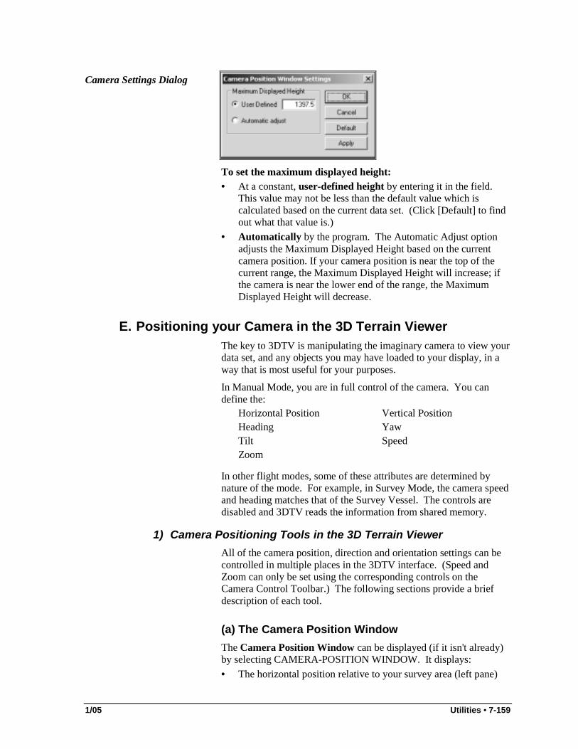
1/05 Utilities • 7-159
Camera Settings Dialog
To set the maximum displayed height: • At a constant, user-defined height by entering it in the field.
This value may not be less than the default value which is calculated based on the current data set. (Click [Default] to find out what that value is.)
• Automatically by the program. The Automatic Adjust option adjusts the Maximum Displayed Height based on the current camera position. If your camera position is near the top of the current range, the Maximum Displayed Height will increase; if the camera is near the lower end of the range, the Maximum Displayed Height will decrease.
E. Positioning your Camera in the 3D Terrain Viewer The key to 3DTV is manipulating the imaginary camera to view your data set, and any objects you may have loaded to your display, in a way that is most useful for your purposes.
In Manual Mode, you are in full control of the camera. You can define the:
Horizontal Position Vertical Position Heading Yaw Tilt Speed Zoom
In other flight modes, some of these attributes are determined by nature of the mode. For example, in Survey Mode, the camera speed and heading matches that of the Survey Vessel. The controls are disabled and 3DTV reads the information from shared memory.
1) Camera Positioning Tools in the 3D Terrain Viewer All of the camera position, direction and orientation settings can be controlled in multiple places in the 3DTV interface. (Speed and Zoom can only be set using the corresponding controls on the Camera Control Toolbar.) The following sections provide a brief description of each tool.
(a) The Camera Position Window The Camera Position Window can be displayed (if it isn't already) by selecting CAMERA-POSITION WINDOW. It displays: • The horizontal position relative to your survey area (left pane)

7-160 • Utilities 1/05
• The vertical position relative to the minimum and maximum depth found in your file (right pane)
• The direction the camera is pointing—both yaw and tilt (green arrow)
• The direction the camera is traveling (red arrow) • The view range (the area between the green lines) • The water level (if it is displayed) • The maximum graph height, which determines the scale of the
graphic.
The displays in each side of the window update to give you visual feedback as you move the camera.
Camera Position Window
(b) Camera Set Position Dialog The Camera Set Position Dialog is accessed by selecting CAMERA-SET POSITION. It enables you to set the horizontal and vertical positioning, as well as the heading of the camera.
Camera Position Dialog
1. Enter the settings for each attribute. 2. Use [Apply] to preview your settings in the 3DTV windows. 3. When you are satisfied, click [OK] to return to the program.
If the camera is moving, when a new position is applied, it immediately changes position and heading according to the new settings, but continues moving at the same speed. Camera Yaw and Tilt are unchanged.
(c) Default Position The Default Position is a composite of all current camera position, direction, and orientation settings. (Zoom and Speed are not included.) At any time, you can save the current settings by clicking

1/05 Utilities • 7-161
[Store Position] and later return the camera to these settings using [Restore Position].
Note: This is only good for 1 set of settings at a time. The stored position is not saved in the project file.
The default position is handy if you see something particularly interesting, or you find that you have an especially good viewing angle, and you want to be able to easily return to that viewing position later.
(d) Camera Controls Camera Controls are contained in the Camera Control tool bar. Each attribute has a labeled control with which you can manipulate the camera. The diagrams and text information provided with each set of controls, gives you detailed information about the status of each setting in the camera controls.
Note: Modes other than Manual Mode predefine some of these attributes and will disable the corresponding controls as noted.
(e) Keyboard Shortcut Commands A set of keyboard shortcuts have been created to replicate all of the camera control functions (except the default positioning feature). Once you are familiar with them, your viewing area can be significantly increased by hiding the Camera Control tool bar. To help you along, a list of the keyboard commands can be accessed by selecting HELP-KEYBOARD SHORTCUTS.
A few of these shortcuts affect camera motion regardless of the type of motion. • [Pause] or Spacebar temporarily stops the camera motion.
When the motion is paused, the text on the button changes to "Resume".
• [Resume] or Spacebar restarts the camera motion at the same speed and rate of turn values as before the pause.
• [Stop] or Ctrl + NumPad 0 permanently stops the camera motion, setting its speed, and turn and elevation rates of change to zero. Stop does not affect Yaw, Tilt, and Zoom controls.
Note: In some cases, to initiate the opposite action, it will be more efficient to click [0] to stop the camera motion, then use the opposite arrow to begin motion in the opposite direction.
(f) Vessel Settings Dialog When a vessel is being displayed, the camera is positioned relative to the boat according to the settings in the Vessel Settings dialog. See the "Vessel Display Options" section.

7-162 • Utilities 1/05
2) Modifying the Camera's Horizontal Position The horizontal positioning is the XY position of the camera.
Tool Procedure
Camera Positioning Window Click in the map view at the position relative to your data where you want the camera.
The red circle will move to that location and the effect will be seen in the 3D Terrain window and in the Side View. This method is quick and easy, is not accurate.
Camera Set Position Dialog Enter the X and Y projection coordinates. Use this option for accurate positioning.
Camera Controls Use the Speed and Turn controls together to navigate your camera in the display. (Turn controls alone will not change the camera position.)
Use the Turn buttons to change the direction the camera moves. Button Function Left and Right Arrows (<- and ->)
Controls the speed of the camera's change in direction of travel Each click increases the turning speed by 1 degree/second.
Zero ( [0] ) Stops the turn. Use the Speed buttons to control how fast (or slowly) it moves.
Button Function Arrow ([<] and [>])
Increment and decrement speed by 1 unit/sec.
Double Arrow ([<<] and [>>])
Increment and decrement speed by 10 units/sec.
Zero ( [0] ) Stops the camera's travel. Camera Speed and Turn Controls

1/05 Utilities • 7-163
Tool Procedure
Keyboard Shortcuts Right Arrow
Ctrl + Right Arrow
Left Arrow
Ctrl + Left Arrow R
Turns +1 degree/second.
Turns +10 degrees/second.
Turns -1 degree/second.
Turns -10 degrees/second. Set turn change to 0.
3) Modifying the Camera's Vertical Position The vertical positioning is the Z coordinate of the camera.
Tool Procedure
Camera Positioning Window Click in the side view of the window at the height, relative to your data, where you want the camera.
The red circle will move to that location and the effect will be seen in the 3D Terrain Window and in the Side View. This method is quick and easy, is not accurate.
Camera Set Position Dialog Enter the Z coordinate. Use this option for fast and accurate positioning.
Camera Controls The Elevation controls adjust the height above the survey area by changing the vertical speed of the camera. Button Function Up and Down Arrows
Increases/decreases the elevation by 1 unit/second. The number of clicks increases/decreases the rate of change (more units/sec.).
Zero ( [0] ) Stops the vertical change. The Arrow buttons increase/decrease the elevation by 1 unit/second for each click. [0] stops the camera at the current height.
Camera Elevation Controls

7-164 • Utilities 1/05
Tool Procedure
Keyboard Shortcuts Up Arrow:
Ctrl + Up Arrow:
Down Arrow:
Ctrl + Down Arrow:
Z
+1 unit/second
+10 units/second
-1 unit/second
-10 units/second
Stop elevation change.
The camera position relative to the depth/elevation range found in your data set is displayed in the Side View graphic. If the camera is outside of the window's range, an arrow will point to the top of the window. The program does not allow you to position the camera lower than the maximum depth found in the current grid cell. (You determined the grid cell size in the Terrain Settings when you began this 3DTV project. They can be edited by selecting TERRAIN- SETTINGS.) If some grid cells are "empty" (there is no data sounding in them), the camera may drop through the terrain.
4) Modifying the Camera Heading As with vessel heading, camera heading is its direction of travel.
Tool Procedure
Camera Positioning Window CTRL + Right click in the map view on the point toward which you want the camera to travel. Drag the mouse with pressed left mouse button to determine direction of the camera (blue arrow will appear). The red camera indicator will be positioned at the point of the left click and move in the direction of the drag.
The effect will be seen in the 3D Terrain Window, in the Heading under the Speed and Turn control, and in the Map View.
Camera Set Position Dialog Enter Heading. A value of 0 is straight up. Use this option for fast and accurate positioning.
Camera Controls The Turn controls determine the direction in which the camera moves. Turn buttons are only enabled in Manual Mode. Button Function Left and Right Arrows (<- and ->)
Controls the speed of the camera's change in direction of travel Each click increases the turning speed by 1 degree/second.
Zero ( [0] ) Stops the turn. The data below the Speed and Turn buttons displays your current settings. The Map View and Camera Position Window also provide a pictorial representation. If the camera position is outside of the Map View, an arrow will point to the window edge to indicate where it is positioned.
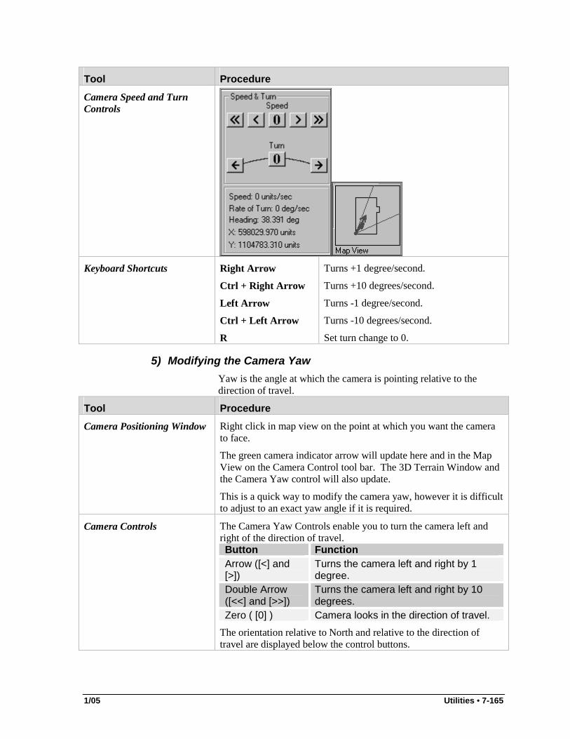
1/05 Utilities • 7-165
Tool Procedure
Camera Speed and Turn Controls
Keyboard Shortcuts Right Arrow
Ctrl + Right Arrow
Left Arrow
Ctrl + Left Arrow
R
Turns +1 degree/second.
Turns +10 degrees/second.
Turns -1 degree/second.
Turns -10 degrees/second.
Set turn change to 0.
5) Modifying the Camera Yaw Yaw is the angle at which the camera is pointing relative to the direction of travel.
Tool Procedure
Camera Positioning Window Right click in map view on the point at which you want the camera to face.
The green camera indicator arrow will update here and in the Map View on the Camera Control tool bar. The 3D Terrain Window and the Camera Yaw control will also update.
This is a quick way to modify the camera yaw, however it is difficult to adjust to an exact yaw angle if it is required.
Camera Controls The Camera Yaw Controls enable you to turn the camera left and right of the direction of travel. Button Function Arrow ([<] and [>])
Turns the camera left and right by 1 degree.
Double Arrow ([<<] and [>>])
Turns the camera left and right by 10 degrees.
Zero ( [0] ) Camera looks in the direction of travel. The orientation relative to North and relative to the direction of travel are displayed below the control buttons.

7-166 • Utilities 1/05
Tool Procedure
Camera Yaw Controls
Keyboard Shortcut NumLock + NumPad 6 NumLock + Ctrl + NumPad 6 NumLock + NumPad 4 NumLock + Ctrl + NumPad 4 NumLock + NumPad 5
Yaw +1 degree Yaw + 10 degrees Yaw – 1 degree Yaw - 10 degrees Yaw and Tilt set to 0.
6) Modifying the Camera Tilt The Camera Tilt adjusts the angle of view relative to the horizon. The tilt angle may range from -180 degrees to 180 degrees.
Tool Procedure
Camera Positioning Window Right click in the side view at the spot to which you want the camera to point.
The green arrow will adjust accordingly. Updates will also occur in the 3D Terrain Window and in the Camera Tilt control.
This method is good to establish the general "pitch" of the camera.
Camera Controls The Camera Tilt controls adjust the tilt. The current setting is displayed below the graphic.
Button Function Arrow Tilts camera up and down by 1 degree/click Double Arrow
Tilts camera up and down by 10 degrees/click
Zero ( [0] ) Tilts camera to 0 degrees. This method is more accurate and is useful for fine tuning your view.

1/05 Utilities • 7-167
Tool Procedure
Camera Tilt Controls
Keyboard Shortcuts NumLock + NumPad 8
NumLock + Ctrl + NumPad 8 NumLock + NumPad 2 NumLock + Ctrl + NumPad 2 NumLock + NumPad 5
Tilt + 1 degree
Tilt + 10 degrees
Tilt - 1 degree
Tilt - 10 degrees
Yaw and Tilt set to 0.
7) Modifying the Camera Speed The Speed controls determine the camera's travel speed. Speed buttons are enabled in Manual Flight, LNW file, and Circle Flight modes.
Tool Procedure
Camera Controls Button Function Arrow ([<] and [>])
Increment and decrement speed by 1 unit/sec.
Double Arrow ([<<] and [>>])
Increment and decrement speed by 10 units/sec.
Zero ( [0] ) Stops the camera's travel.
Keyboard Shortcuts NumPad –
NumPad +
S
Decrease Speed by 1 unit/second
Increase Speed by 1 unit/second
Sets Speed to 0.
8) Modifying the Camera Zoom Tool Procedure
Camera Control The Camera Zoom slide control adjusts the range of view. (This is similar to the standard snap shot versus wide angle and panoramic shots with a still life camera.) The current angle is printed below the slide control. [Default] snaps the angle to 45 degrees.
The Map View and Camera Position Window show the view range (the area between the green lines) .

7-168 • Utilities 1/05
Tool Procedure
Camera Zoom Controls
Keyboard Shortcuts NumPad /
NumPad *
Zoom In
Zoom Out
F. Saving your Views in the 3D Terrain Viewer In 3DTV, you can save screen captures of your data or you can record and replay a specialized 3DTV movie of your display.
1) Exporting a Screen Capture You can quickly and easily take a screen capture of your 3D Terrain Window by selecting TOOLS-TAKE A SNAPSHOT or by clicking the corresponding icon in the Accessories Toolbar. The Windows® File Save dialog will appear for you to name the file. You can choose to save it as a JPG, BMP or TIF file.
2) Recording a 3D Terrain Viewer Movie The Movie Control Toolbar enables you to save a record of your camera's travel so it can later replay what it viewed. (Hold the cursor over any button and the function is displayed in the status bar at the bottom of the window.)
Camera Movie Controls
Record a movie by clicking the record button (or TOOLS-RECORD MOVIE) then use the camera controls to scan the area.
Note: In Matrix 3DTV mode, when the vessel passes from one MTX file to another, the movie recording will be stopped automatically. You can save the recorded movie or to start recording again.
Pause the recording by clicking the pause button on the movie toolbar. This can be useful if you're viewing an area that's of no particular interest. The camera motion will continue while the movie is paused.
Resume recording by clicking the same button again.

1/05 Utilities • 7-169
Stop recording by clicking the stop button on the movie toolbar.
Save your movie, when you are satisfied with what you recorded, by clicking [Save]. 3DTV will display a File Save dialog for you to name your file. The information will be saved to a *.3DM file. The File Save dialog will first default to your project directory, but you may choose another location. Each save after that will default to the last save location chosen.
Replay your movie by clicking [Load] (or TOOLS-LOAD MOVIE) and selecting the 3DM file. • Play the movie in the same amount of time by clicking the
play button (or MOVIE-PLAYBACK). • Manually scan your movie by dragging the slide button across
the toolbar. This is helpful if you want to review certain portions of the movie without taking the time to see the whole recording. It also enables you to move back and forth through your data. After positioning to the desired frame of the movie, you can start replaying the movie from that point by clicking the Play button. Manual scanning is disabled while a movie is being replayed.
• Pause the movie playback by clicking the Pause button on the movie toolbar. Resume playback by pressing the Pause button again.
Note: Movie playback will work only for the same terrain data as were loaded when movie is recorded. You can not load movie recorded above other terrains.
3) Recording to an AVI File You can also record the output of the most recently activated Terrain window into an AVI file which can be viewed using media player software. • Begin recording by selecting TOOLS-RECORD AVI, or
clicking the AVI icon on the Accessories toolbar. • Stop recording by selecting TOOLS-STOP AVI, or clicking the
AVI icon on the Accessories toolbar. A File Save dialog will appear for you to name your file.
Note: While AVI file recording is in progress, the corresponding 3D Terrain Window will not be resizable (manually or through minimize/maximize buttons).
Before recording your file, you can set the quality of the resulting AVI display. Access the AVI Options dialog by selecting TOOLS-AVI OPTIONS.
The Compressor Quality slide controls the resolution of the resulting AVI display. A higher quality setting results in a larger file with improved resolution.
The Temporary File Path determines where your AVI file is stored while you're recording. When the recording is finished, a File Save

7-170 • Utilities 1/05
dialog will appear for you to name the file and path. The file is renamed and moved.
AVI Options
There are few issues that should be aware of as you consider AVI recording: • A smaller Terrain window will result in a smaller AVI file. • A smaller Terrain window allow faster AVI capture.
Unfortunately, the speed at which the terrain is being rendered depends on the complexity of the model (the size of the dataset).
• AVI recording is a CPU intensive operation, much like terrain rendering. Thus, when the AVI is being recorded, the rate at which terrain windows present a complex terrain model will inevitably be lower than usual. You may see now difference even when using simple models depending on your hardware capabilities.
• 3DTV only records changes in the window from which contents are being captured. Thus, for example, if the camera holds still, the AVI file will be quite small.
G. Optimizing 3D Terrain View Performance A number of options are provided under the View menu that allow you to optimize the function of 3DTV on your computer. The following sections, provide a brief description of each option. You may need to do a bit of experimenting to find the best settings for your equipment.
1) Graphical User Interface Response Mode GUI Response mode affects the speed of the response to your interaction with the interface controls versus the speed that the terrain is updated and redrawn when you are using very large data sets.
In Fast Response mode, the interface responds immediately while the program simultaneously continues to refresh your terrain when camera moves (e.g. camera control buttons work, terrain picture changes while camera is moving and menu is opened). If you are using a very large data set, the display rate is slightly lower in this mode. Some video cards are unreliable in this mode.
Use the Safe Response mode when you load a large data set if:
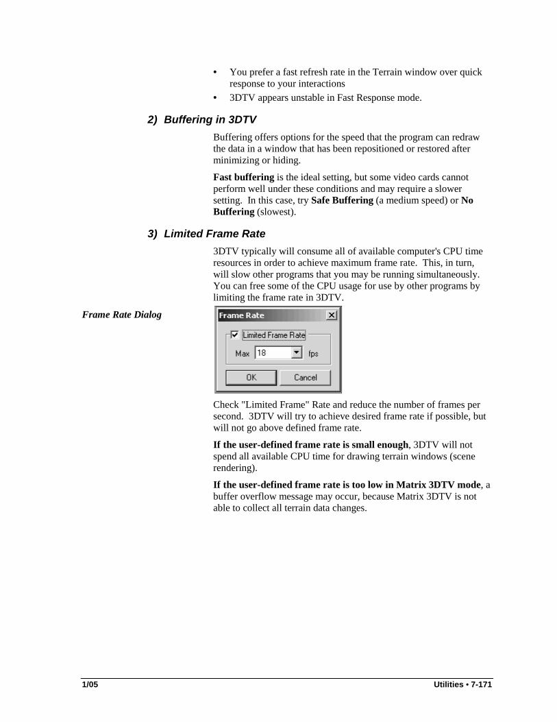
1/05 Utilities • 7-171
• You prefer a fast refresh rate in the Terrain window over quick response to your interactions
• 3DTV appears unstable in Fast Response mode.
2) Buffering in 3DTV Buffering offers options for the speed that the program can redraw the data in a window that has been repositioned or restored after minimizing or hiding.
Fast buffering is the ideal setting, but some video cards cannot perform well under these conditions and may require a slower setting. In this case, try Safe Buffering (a medium speed) or No Buffering (slowest).
3) Limited Frame Rate 3DTV typically will consume all of available computer's CPU time resources in order to achieve maximum frame rate. This, in turn, will slow other programs that you may be running simultaneously. You can free some of the CPU usage for use by other programs by limiting the frame rate in 3DTV.
Frame Rate Dialog
Check "Limited Frame" Rate and reduce the number of frames per second. 3DTV will try to achieve desired frame rate if possible, but will not go above defined frame rate.
If the user-defined frame rate is small enough, 3DTV will not spend all available CPU time for drawing terrain windows (scene rendering).
If the user-defined frame rate is too low in Matrix 3DTV mode, a buffer overflow message may occur, because Matrix 3DTV is not able to collect all terrain data changes.