15 Nov. 200015-859B - Introduction to Scientific Computing1 Multigrid Methods and Applications Paul Heckbert Computer Science Department Carnegie Mellon

15 Nov. 2000 15-859B - Introduction to Scientific Computing 1

Multigrid Methodsand Applications

Paul Heckbert

Computer Science Department

Carnegie Mellon University


Overview

1. What is the multigrid method?

2. High level survey of applications of multigrid methods across science and engineering. (Articles on this are hard to find!)

– what is the state of the art?

– what are multigrid’s strengths & weaknesses?

– what is current research?


Inspiration for Multigrid Method

• Typical problem:– Solving a PDE over simple domain (e.g. square)

– Get sparse system Av=f

• If we solve iteratively with Gauss-Seidel– initial iterations reduce residual a lot

– later iterations yield less benefit

– why? Iterations reduce high frequencies in residual

• Idea:– iterate on coarser grids to reduce lower frequencies


Example: Poisson’s Equation

• Sweep of Gauss-Seidel “relaxes” each grid value to be the average of its four neighbors plus an f offset

• Many relaxations required to solve this on a fixed grid.

• Multigrid solves it on a hierarchy of grids.

2

,

21, , 1 , , 1 1, ,

( , ), solve for ( , )

discretize ( , )

[ 4 ]/

i j

i j i j i j i j i j i j

u f x y u x y

v u ih jh

v v v v v h f


Elements of Multigrid Method

• relax on a given grid a few times

• coarsen (restrict) a grid

• refine (interpolate) a grid


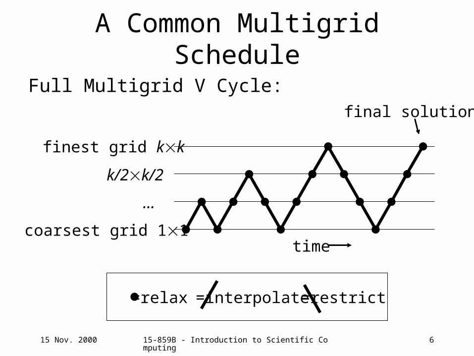
A Common Multigrid Schedule

Full Multigrid V Cycle:

timecoarsest grid 11

finest grid kk

k/2k/2

...

final solution

=relax =interpolate =restrict


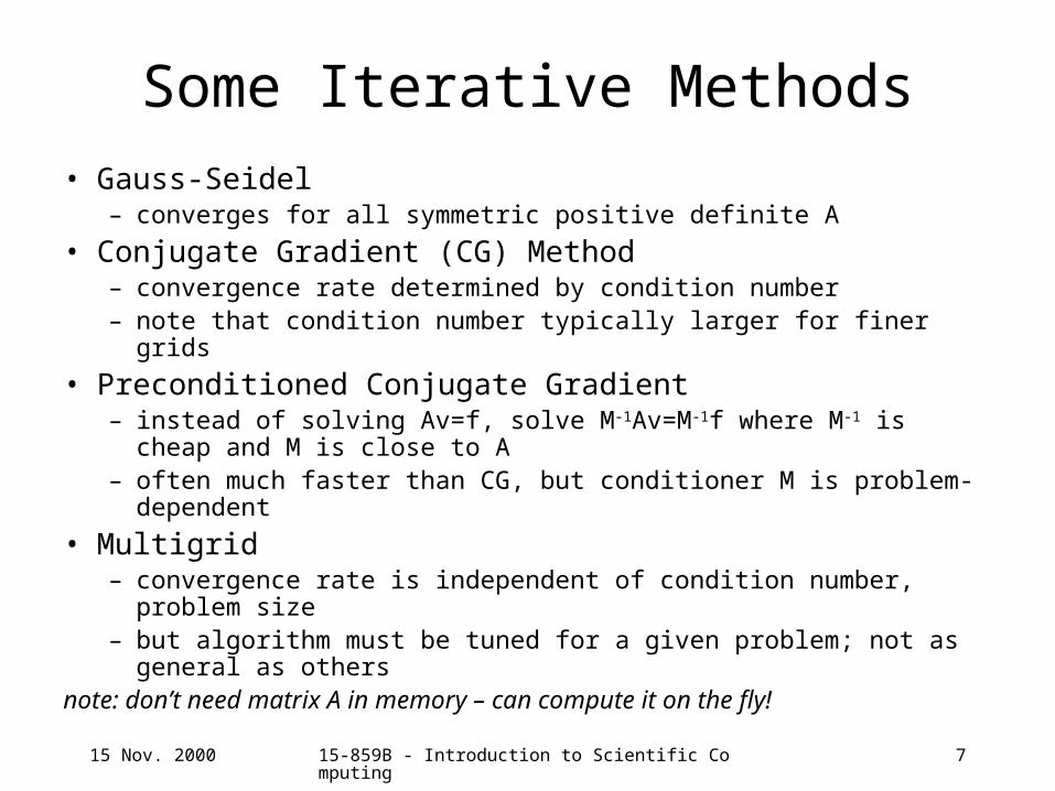
Some Iterative Methods

• Gauss-Seidel– converges for all symmetric positive definite A

• Conjugate Gradient (CG) Method– convergence rate determined by condition number– note that condition number typically larger for finer grids

• Preconditioned Conjugate Gradient– instead of solving Av=f, solve M-1Av=M-1f where M-1 is cheap and M

is close to A– often much faster than CG, but conditioner M is problem-dependent

• Multigrid– convergence rate is independent of condition number, problem size– but algorithm must be tuned for a given problem; not as general as

othersnote: don’t need matrix A in memory – can compute it on the fly!


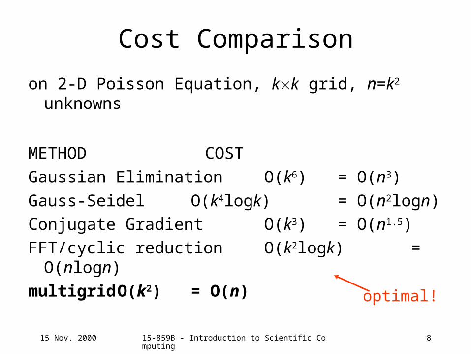
Cost Comparison

on 2-D Poisson Equation, kk grid, n=k2 unknowns

METHOD COST

Gaussian Elimination O(k6) = O(n3)

Gauss-Seidel O(k4logk) = O(n2logn)

Conjugate Gradient O(k3) = O(n1.5)

FFT/cyclic reduction O(k2logk) = O(nlogn)

multigrid O(k2) = O(n)optimal!


Memory Requirements of Multigrid

2-D:finest grid: k2 (v & f arrays)

k2/4

k2/16

...

coarsest grid: 1

total: k2(1+1/4+1/16+1/64+...) = 4/3k2

Costs only 33% more memory than storing the solution


Critique of Multigrid 1

• works well for certain problems– in particular, elliptic PDE's (linear or nonlinear) with smooth boundary– solves a problem with n unknowns in O(n) time

• constants usually small, e.g. 10 "work units"• 1 work unit = the work of one relaxation on the fine grid

• but multigrid methods are currently several orders of magnitude slower for non-elliptic steady-state (time-independent BV) problems

• low memory requirements: need mem for v & f on finest grid, plus coarser grids; don’t need A

• parallelizes easily– (but requires more communication than some other parallel

solvers)


Critique of Multigrid 2

• less theory than some other methods– it's a bit of a black art

• requires careful tuning to get it working on a new problem– not a black box, like, say, the conjugate gradient method or Gauss-

Seidel

– but when it works well, it's often the fastest

• but other fast methods often require tuning too– to get top performance out of the conjugate gradient method often

requires an application-specific preconditioner


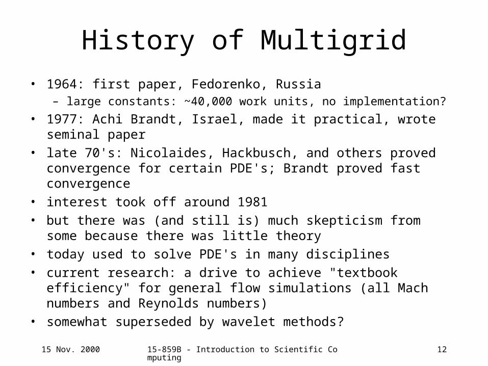
History of Multigrid

• 1964: first paper, Fedorenko, Russia– large constants: ~40,000 work units, no implementation?

• 1977: Achi Brandt, Israel, made it practical, wrote seminal paper

• late 70's: Nicolaides, Hackbusch, and others proved convergence for certain PDE's; Brandt proved fast convergence

• interest took off around 1981

• but there was (and still is) much skepticism from some because there was little theory

• today used to solve PDE's in many disciplines

• current research: a drive to achieve "textbook efficiency" for general flow simulations (all Mach numbers and Reynolds numbers)

• somewhat superseded by wavelet methods?


Multigrid Guidelines

• “multigridders” prefer structured grids

• grid and relaxation method are the only parts of the method that are highly problem-dependent; restriction and interpolation are generic

• on complex domains, need extra relaxation steps near boundary– for rough boundary conditions

– for concave corners

• grid can be adaptive: can restrict processing at finer levels to subdomains

• schedule parameters (how many relaxation steps and V cycles) can be:– fixed

– accommodativee.g. software loops until residual at each step is below some tolerance

• for CFD, align the grid with the boundary and the flow


Brandt’s Research Philosophy

• To do multigrid research, you should "very gradually increase the complexity of the problems” you attempt

• "we insist on obtaining for each problem the full efficiency” (e.g. 10 work units)

• strives for linear time with small constants• "stalling numerical processes must be wrong”• constants are particularly important when discussing

algorithms that are O(n); more than for algorithms that are, say, O(n2)

• strives for convergence proofs with small constants: “almost all other multigrid theories give estimates which are not quantitative or very unrealistic, rendering them useless in practice”


Computational Fluid Dynamics (CFD)

• equations– Euler equation - linear, inviscid (no viscosity)

– Navier-Stokes equation - nonlinear, models viscosity

• now possible to simulate flow around an airplane, with engines

– first achieved in 1986

– done with multigrid?

• Reynolds Number (Re)

– a measure of the ratio of inertial and viscous forces

– Re large => turbulence, difficult simulation

– for an airplane, Re ~ 10^7


CFD 2

• transonic flow

– flow is both below and above speed of sound (Mach no. <1 or >1)

– => PDE is elliptic where subsonic and hyperbolic where supersonic

• high Reynolds number steady state flows

=> non-elliptic

• use boundary-fitted structured grids

• boundary layer tricky– in viscous simulation, flow near surface (of e.g. wing) has high gradient, since

flow speed at surface is zero, but speed inches away could be high

– you often want the elements (grid quadrilaterals) to be highly stretched (e.g. "aspect ratio" of 4000:1) in boundary layer to get accurate simulations

– high aspect ratio slows convergence or complicates the relaxation method


Multigrid Applications 1

• computational fluid dynamics (CFD)– application for which multigrid has been most used– weather prediction (whole earth simulations)

• structured grid generation– use elliptic PDE to define geometry of grid nodes, create grid using

multigrid!

• ill-posed (underdetermined) problems– edge detection in noisy image

• can find all straight features (lines, edges) in kxk pixel image in O(k log k) time

– image segmentation– tomography (i.e. CAT scan)– approximating noisy data with a piecewise smooth function with

known or unknown discontinuities



• integral operators– multiplication by a dense nxn matrix in O(n) time

– easy if matrix (or kernel) is smooth; slower if not

– n-body force computations• gravity

• molecular interactions

• thermal radiation

– Fast Multipole Method is faster than O(n2) alg. only for n>1000, they say

• is Brandt's method faster? (unpublished)



• global optimization– works even if many local minima

– "each step can be interpreted as an optimization over a certain subspace"

– protein folding

• constrained optimization– optimal control, e.g. robot motion planning

• solid mechanics– set up using finite element methods (unstructured grid), not finite

difference



• quantum chemistry– compute eigenfunctions of Schroedinger's eqn. (the PDE governing

quantum mechanics) to find electron density functions

• macroscopic from microscopic– statistical physics, particle physics (QCD)

• derive macroscopic properties (e.g. nonlinear elasticity) by using multigrid on microscopic level (on atomic forces)

– unified wave/ray methods for simulating electromagnetic radiation• combine wave model (to simulate diffraction, interference, when

wavelength comparable to scale of objects) and

• ray model (to simulate free flight of photons in air/vacuum)

• VLSI design– highly nonlinear


Related Methods

• unstructured multigrid– uses an unstructured grid (irregular topology), not structured one

– this complicates relaxation, restriction, & interpolation, but permits solution on complex domains (e.g. around an aircraft wing with flaps)

• algebraic multigrid– multigrid without the grid

– analyze and do clustering on graph implied by matrix A

– input is A only -- no high level problem knowledge

• domain decomposition– divide domain into (possibly overlapping) pieces

– solve alternately on each piece, using solution of other pieces as boundary conditions

– useful for complex domains, parallelizes easily


References 1

my comments in italics

Brandt, 1988, The Weizmann Insitute Research in Multilevel Computation: 1988 Report, Proc. Copper Mtn. Conf. on Multigrid Methods, 1989 (53 pp.) Survey of recent applications. I found this quite thought-provoking.

Brandt, 1982, Guide to Multigrid Development, in Hackbusch & Trottenberg, eds., Multigrid Methods, pp. 220-312. Guidelines for multigrid implementers. Long.

Brandt, 1997, The Gauss Center Research in Multiscale Scientific Computation, Proc. Copper Mtn. Conf. on Multigrid Methods, on web (50 pp.) http://www.wisdom.weizmann.ac.il/research.html More esoteric than 1988 report above.

Brandt, 1980, Multilevel Adaptive Computations in Fluid Dynamics, AIAA J., vol. 18, pp. 1165-1172. Short, fairly readable.

Brandt, 1977, Multi-Level Adaptive Solutions to Boundary-Value Problems, Mathematics of Computation, pp. 333-390. The seminal paper on multigrid.


References 2Wesseling, 1992, An Intro. to Multigrid Methods, chapter 8. Good textbook.

Parsons & Hall 1990, The Multigrid Method in Solid Mechanics, Intl. J. for Numer. Meth. in Eng., vol. 29, pp. 719-754. Experiments applying MG to mechanical engineering.

Chan, Go, & Zikatanov, 1997, Lecture Notes on Multilevel Methods for Elliptic Problems on Unstructured Grids, 77 pp., http://www.math.ucla.edu/~chan/mgpapers.html State of the art in unstructured multigrid and domain decomposition.

Shlomo Ta’asan, CMU Math (conversation)

Gary Miller, CMU CS (conversation)

Omar Ghattas, CMU CE (conversation)

Documents

15 Nov. 200015-859B - Introduction to Scientific Computing1 Multigrid Methods and Applications Paul Heckbert Computer Science Department Carnegie Mellon