Embed Size (px)
Citation preview
2/36
Probability
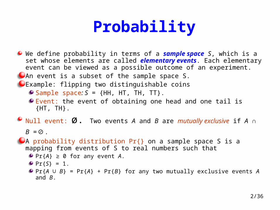
We define probability in terms of a sample space S, which is a set whose elements are called elementary events. Each elementary event can be viewed as a possible outcome of an experiment. An event is a subset of the sample space S.Example: flipping two distinguishable coins
Sample space: S = {HH, HT, TH, TT}.Event: the event of obtaining one head and one tail is {HT, TH}.
Null event: ø. Two events A and B are mutually exclusive if A ∩ B = .⊘ A probability distribution Pr{} on a sample space S is a mapping from events of S to real numbers such that
Pr{A} ≥ 0 for any event A.Pr{S} = 1.Pr{A ∪ B} = Pr{A} + Pr{B} for any two mutually exclusive events A and B.
3/36
Axioms of probability
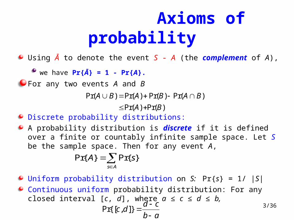
Using Ā to denote the event S - A (the complement of A),
we have Pr{Ā} = 1 - Pr{A}. For any two events A and B
Discrete probability distributions:
A probability distribution is discrete if it is defined over a finite or countably infinite sample space. Let S be the sample space. Then for any event A,
Uniform probability distribution on S: Pr{s} = 1/ |S|
Continuous uniform probability distribution: For any closed interval [c, d], where a ≤ c ≤ d ≤ b,
Pr( ) Pr( ) Pr( ) Pr( )
Pr( ) Pr( )
A B A B A B
A B
Pr{ } Pr{ }s A
A s
Pr{[ , ]}d c
c db a
4/36
Probability
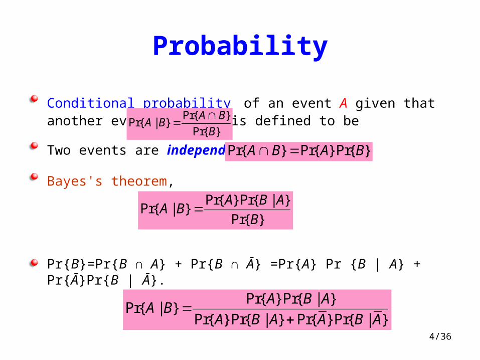
Conditional probability of an event A given that another event B occurs is defined to be
Two events are independent if
Bayes's theorem,
Pr{B}=Pr{B ∩ A} + Pr{B ∩ Ā} =Pr{A} Pr {B | A} + Pr{Ā}Pr{B | Ā}.
Pr{ }Pr{ | }
Pr{ }
A BA B
B
Pr{ } Pr{ }Pr{ }A B A B
Pr{ }Pr{ | }Pr{ | }
Pr{ }
A B AA B
B
Pr{ }Pr{ | }Pr{ | }
Pr{ }Pr{ | } Pr{ }Pr{ | }
A B AA B
A B A A B A
5/36
Discrete random variables
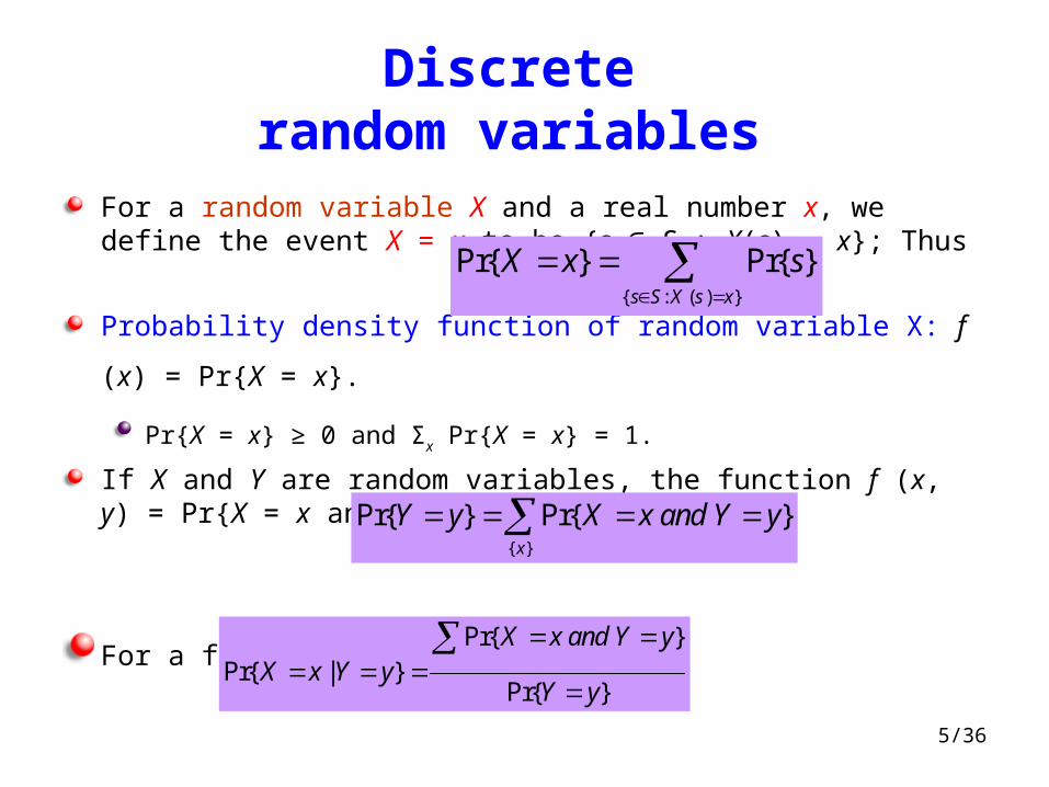
For a random variable X and a real number x, we define the event X = x to be {s ∈ S : X(s) = x}; Thus
Probability density function of random variable X: f (x) = Pr{X = x}. Pr{X = x} ≥ 0 and Σx Pr{X = x} = 1.
If X and Y are random variables, the function f (x, y) = Pr{X = x and Y = y}
For a fixed value y,
{ : ( ) }
Pr{ } Pr{ }s S X s x
X x s
{ }
Pr{ } Pr{ }x
Y y X x and Y y
Pr{ }Pr{ | }
Pr{ }
X x and Y yX x Y y
Y y

6/36
Expected value of a random variable
Expected value (or, synonymously, expectation or mean) of a discrete random variable X is
Example: Consider a game in which you flip two fair coins. You earn $3 for each head but lose $2 for each tail. The expected value of the random variable X representing your earnings is
E[X] = 6 · Pr{2 H's} + 1 · Pr{1 H, 1 T} - 4 · Pr{2 T's} =6(1/4) + 1(1/2) - 4(1/4) =1.
Linearity of expectation:
when n random variables X1, X2,..., Xn are mutually independent,
[ ] Pr{ }x
E X x X x
[ ] [ ] [ ]E X Y E X E Y
1 2 1 2[ ] [ ] [ ] [ ]n nE X X X E X E X E X
7/36
First success
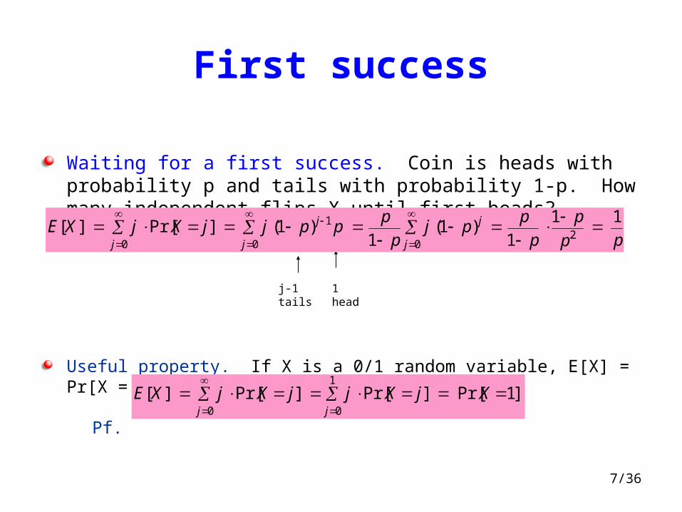
Waiting for a first success. Coin is heads with probability p and tails with probability 1-p. How many independent flips X until first heads?
Useful property. If X is a 0/1 random variable, E[X] = Pr[X = 1].
Pf.
j-1 tails
1 head
E[X ] j Pr[X j]j0
j (1 p) j1 p
j0
p
1 pj (1 p) j
j0
p
1 p1 p
p2 1
p
E[X ] j Pr[X j]j0
j Pr[X j]
j0
1 Pr[X 1]
8/36
Variance and standard deviation
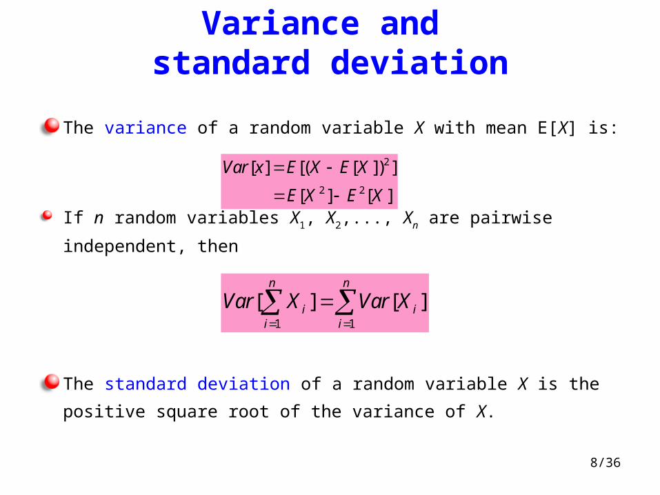
The variance of a random variable X with mean E[X] is:
If n random variables X1, X2,..., Xn are pairwise independent, then
The standard deviation of a random variable X is the positive square root of
the variance of X.
2
2 2
[ ] [( [ ]) ]
[ ] [ ]
Var x E X E X
E X E X
1 1
[ ] [ ]n n
i ii i
Var X Var X
9/36
Randomization
Randomization. Allow fair coin flip in unit time.
Why randomize? Can lead to simplest, fastest, or only known algorithm for a particular problem.
Ex. Symmetry breaking protocols, graph algorithms, quicksort, hashing, load balancing, Monte Carlo integration, cryptography.
10/36
Maximum 3-Satisfiability
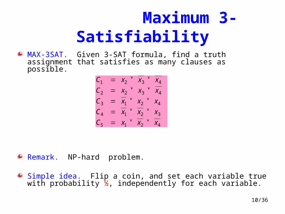
MAX-3SAT. Given 3-SAT formula, find a truth assignment that satisfies as many clauses as possible.
Remark. NP-hard problem.
Simple idea. Flip a coin, and set each variable true with probability ½, independently for each variable.
C1 x2 x3 x4
C2 x2 x3 x4
C3 x1 x2 x4
C4 x1 x2 x3
C5 x1 x2 x4
11/36
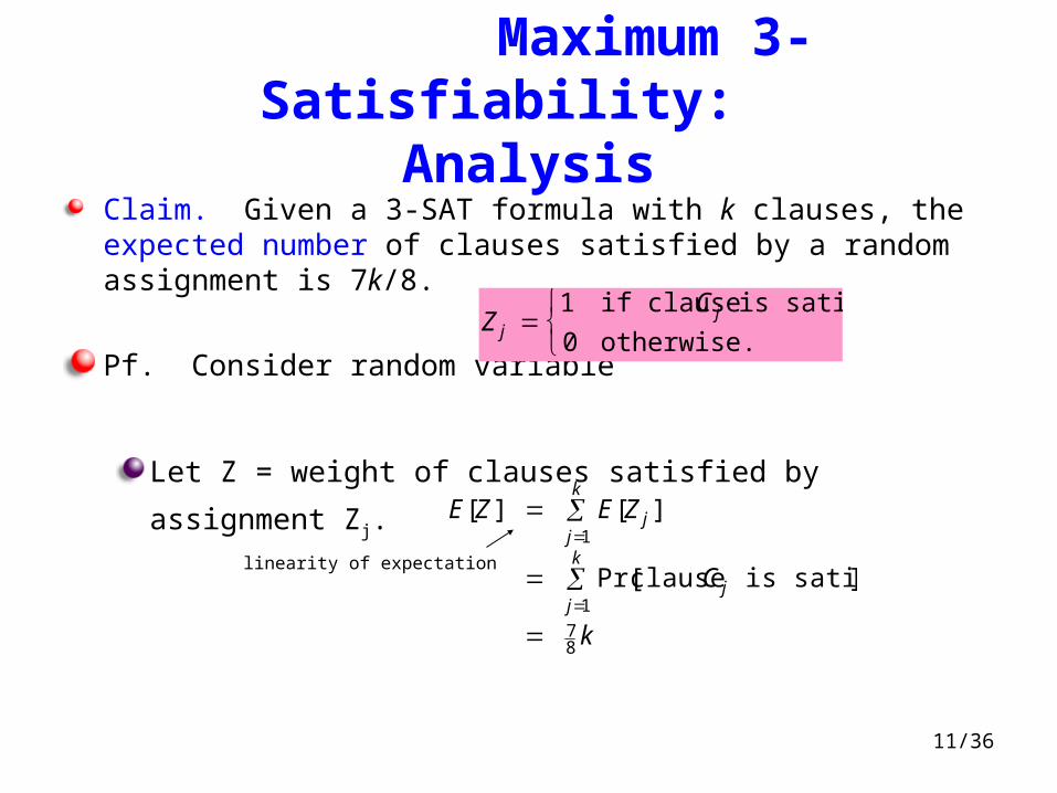
Claim. Given a 3-SAT formula with k clauses, the expected number of clauses satisfied by a random assignment is 7k/8.
Pf. Consider random variable
Let Z = weight of clauses satisfied by assignment Zj.
E[Z ] E[Z jj1
k ]
Pr[clause C j is satisfiedj1
k ]
78 k
Maximum 3-Satisfiability: Analysis
Z j 1 if clause C j is satisfied
0 otherwise.
linearity of expectation
12/36
E[Zj]
E[Zj] is equal to the probability that Cj is satisfied.
Cj is not satisfied, each of its three variables must be assigned the value that fails to make it true, since the variables are set independently, the probability of this is (1/2)3=1/8. Thus Cj is satisfied with probability 1 – 1/8 = 7/8.
Thus E[Zj] = 7/8.
13/36
Maximum 3-SAT: Analysis
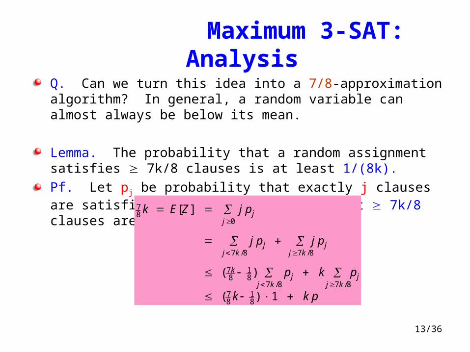
Q. Can we turn this idea into a 7/8-approximation algorithm? In general, a random variable can almost always be below its mean.
Lemma. The probability that a random assignment satisfies 7k/8 clauses is at least 1/(8k).
Pf. Let pj be probability that exactly j clauses are satisfied; let p be probability that 7k/8 clauses are satisfied.
78 k E[Z ] j p j
j 0
j p j j p jj 7k /8
j 7k /8
( 7k8 1
8 ) p j k p jj 7k /8
j 7k /8
( 78 k 1
8 ) 1 k p
14/36
Analysis con.
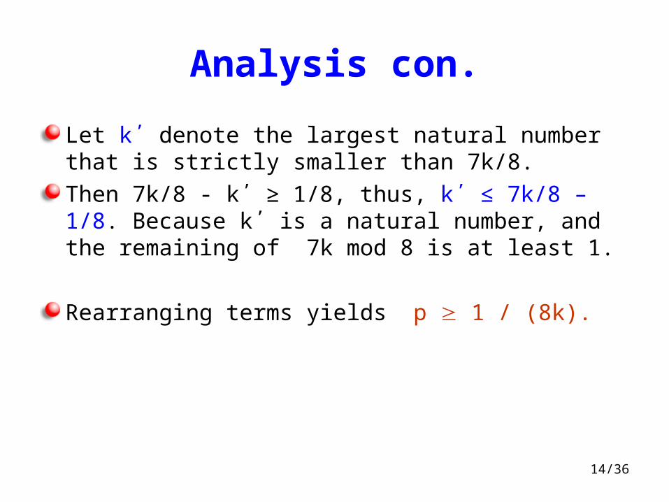
Let k΄ denote the largest natural number that is strictly smaller than 7k/8.
Then 7k/8 - k΄ ≥ 1/8, thus, k΄ ≤ 7k/8 – 1/8. Because k΄ is a natural number, and the remaining of 7k mod 8 is at least 1.
Rearranging terms yields p 1 / (8k).
15/36
Maximum 3-SAT: Analysis
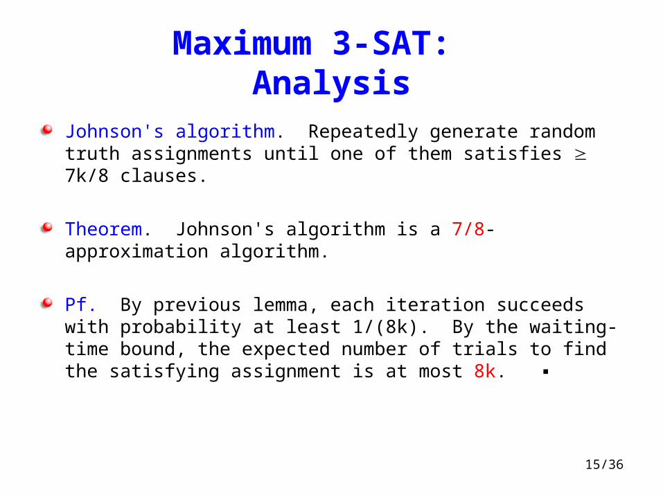
Johnson's algorithm. Repeatedly generate random truth assignments until one of them satisfies 7k/8 clauses.
Theorem. Johnson's algorithm is a 7/8-approximation algorithm.
Pf. By previous lemma, each iteration succeeds with probability at least 1/(8k). By the waiting-time bound, the expected number of trials to find the satisfying assignment is at most 8k. ▪
16/36
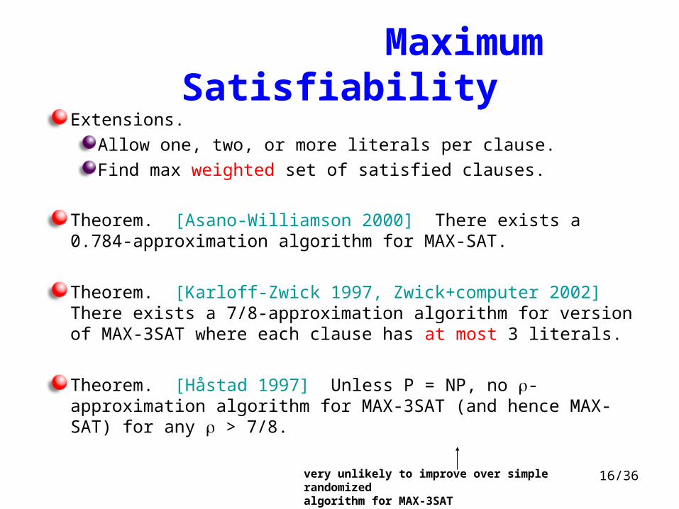
Maximum SatisfiabilityExtensions.
Allow one, two, or more literals per clause.
Find max weighted set of satisfied clauses.
Theorem. [Asano-Williamson 2000] There exists a 0.784-approximation algorithm for MAX-SAT.
Theorem. [Karloff-Zwick 1997, Zwick+computer 2002] There exists a 7/8-approximation algorithm for version of MAX-3SAT where each clause has at most 3 literals.
Theorem. [Håstad 1997] Unless P = NP, no -approximation algorithm for MAX-3SAT (and hence MAX-SAT) for any > 7/8.
very unlikely to improve over simple randomizedalgorithm for MAX-3SAT
17/36
Randomized Divide-and-Conquer
18/36
Finding the Median
We are given a set of n numbers S={a1,a2,...,an}.
The median is the number that would be in the middle position if we were to sort them.
The median of S is equal to kth largest element in S, where
k = (n+1)/2 if n is odd, and k=n/2 if n is even.
Remark. O(n log n) time if we simply sort the number first.
Question: Can we improve it?

19/36
Selection problem
Selection problem. Given a set of n numbers S and a number k between 1 and n. Return the kth largest element in S.
Select (S, k)choose a splitter ai S uniformly at random foreach (a S) { if (a < ai) put a in S-
else if (a > ai) put a in S+
}If |S-|=k-1 then ai was the desired answerElse if |S-|≥k-1 then The kth largest element lies in S-
Recursively call Select(S-,k)Else suppose |S-|=l < k-1 then The kth largest element lies in S+ Recursively call Select(S+,k-1-l)Endif
20/36
Analysis
Remark. Regardless how the splitter is chosen, the algorithm above returns the kth largest element of S.Choosing a good Splitter.
A good choice: a splitter should produce sets S- and S+ that are approximately equal in size.For example: we always choose the median as the splitter. Then each iteration, the size of problem shrink half. Let cn be the running time for selecting a uniformed number. Then the running time isT(n) ≤ T(n/2) + cnHence T(n) = O(n).
21/36
Analysis con.
Funny!! The median is just what we want to find. However, if for any fixed constant b > 0, the size of sets in the recursive call would shrink by a factor of at least (1- b) each time. Thus the running time T(n) would be bounded by the recurrence T(n) ≤ T((1-b)n) + cn. We could also get T(n) = O(n).
A bad choice. If we always chose the minimum element as the splitter, then T(n) ≤ T(n-1) + cnWhich implies that T(n) = O(n2).

22/36
Random Splitters
However, we choose the splitters randomly.
How should we analysis the running time of this performance?
Key idea. We expect the size of the set under consideration to go down by a fixed constant fraction every iteration, so we would get a convergent series and hence a linear bound running time.
23/36
Analyzing the randomized algorithm
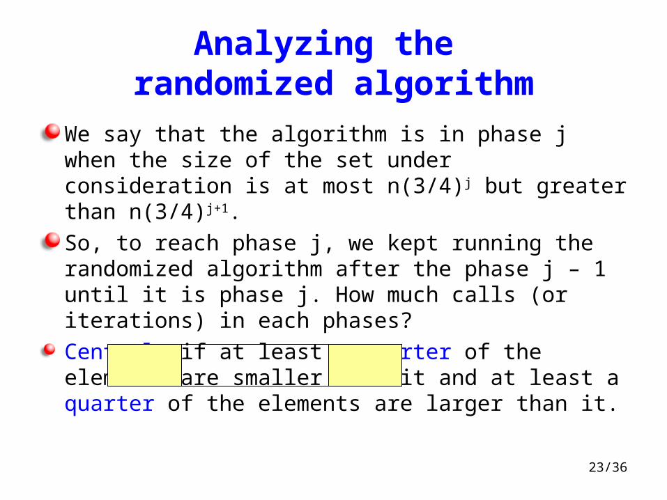
We say that the algorithm is in phase j when the size of the set under consideration is at most n(3/4)j but greater than n(3/4)j+1.
So, to reach phase j, we kept running the randomized algorithm after the phase j – 1 until it is phase j. How much calls (or iterations) in each phases?
Central: if at least a quarter of the elements are smaller than it and at least a quarter of the elements are larger than it.
24/36
Analyzing
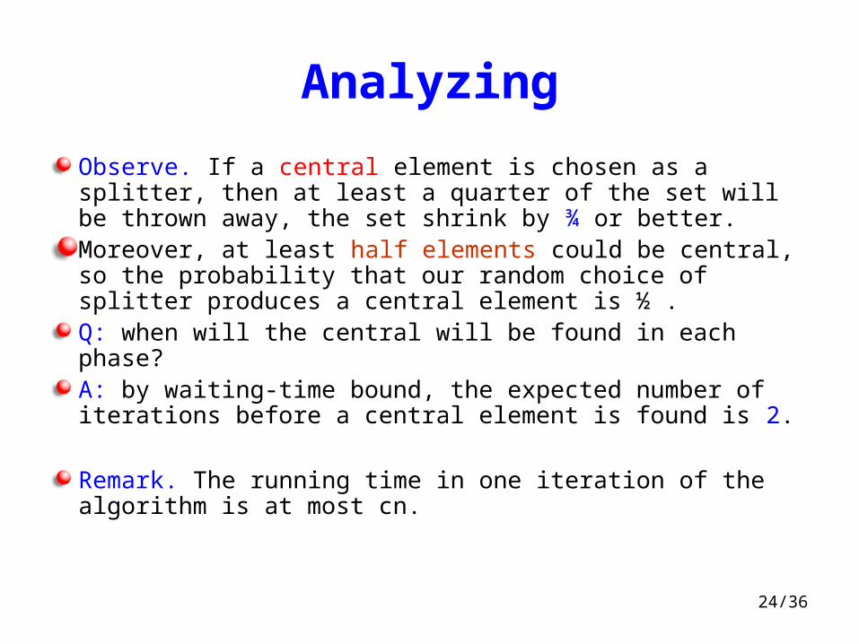
Observe. If a central element is chosen as a splitter, then at least a quarter of the set will be thrown away, the set shrink by ¾ or better.Moreover, at least half elements could be central, so the probability that our random choice of splitter produces a central element is ½ . Q: when will the central will be found in each phase?A: by waiting-time bound, the expected number of iterations before a central element is found is 2.
Remark. The running time in one iteration of the algorithm is at most cn.
25/36
Analyzing
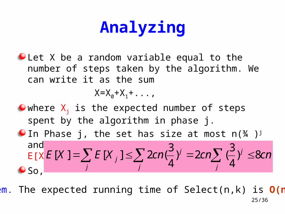
Let X be a random variable equal to the number of steps taken by the algorithm. We can write it as the sum
X=X0+X1+...,
where Xj is the expected number of steps spent by the algorithm in phase j.
In Phase j, the set has size at most n(¾ )j and the number of iterations is 2, thus, E[Xj] ≤ 2 cn(¾ )j
So,
cncncnXEXE
j
j
j
j
jj 8)
4
3(2)
4
3(2][][
Theorem. The expected running time of Select(n,k) is O(n).
26
Contention Resolution
in a Distributed System
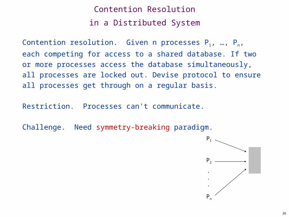
Contention resolution. Given n processes P1, …, Pn, each
competing for access to a shared database. If two or more processes access the database simultaneously, all processes are locked out. Devise protocol to ensure all processes get through on a regular basis.
Restriction. Processes can't communicate.
Challenge. Need symmetry-breaking paradigm.
P1
P2
Pn
.
.
.
27
Contention Resolution:
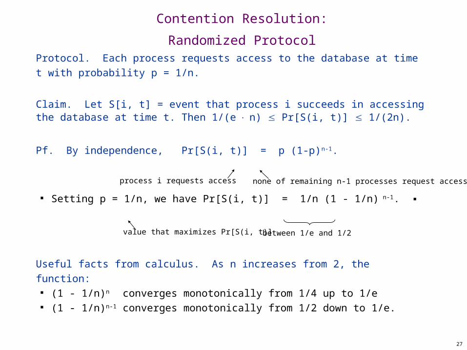
Randomized ProtocolProtocol. Each process requests access to the database at time t with probability p = 1/n.
Claim. Let S[i, t] = event that process i succeeds in accessing the database at time t. Then 1/(e n) Pr[S(i, t)] 1/(2n).
Pf. By independence, Pr[S(i, t)] = p (1-p)n-1.
Setting p = 1/n, we have Pr[S(i, t)] = 1/n (1 - 1/n) n-1. ▪
Useful facts from calculus. As n increases from 2, the function: (1 - 1/n)n-1 converges monotonically from 1/4 up to 1/e (1 - 1/n)n-1 converges monotonically from 1/2 down to 1/e.
process i requests access none of remaining n-1 processes request access
value that maximizes Pr[S(i, t)] between 1/e and 1/2
28
Contention Resolution: Randomized Protocol
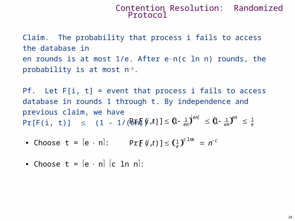
Claim. The probability that process i fails to access the database inen rounds is at most 1/e. After en(c ln n) rounds, the probability is at most n-c.
Pf. Let F[i, t] = event that process i fails to access database in rounds 1 through t. By independence and previous claim, we havePr[F(i, t)] (1 - 1/(en)) t.
Choose t = e n:
Choose t = e n c ln n:
Pr[F(i, t)] 1 1en en
1 1en en
1e
Pr[F(i, t)] 1e c ln n
n c
29
Contention Resolution: Randomized Protocol
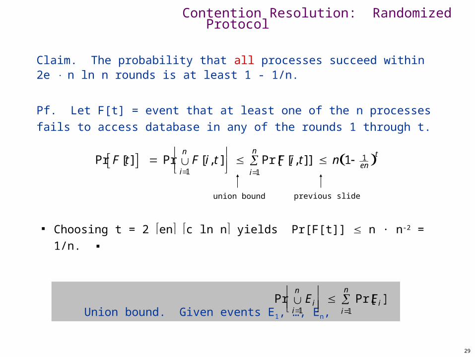
Claim. The probability that all processes succeed within 2e n ln
n rounds is at least 1 - 1/n.
Pf. Let F[t] = event that at least one of the n processes fails to access database in any of the rounds 1 through t.
Choosing t = 2 en c ln n yields Pr[F[t]] n · n-2 = 1/n. ▪
Union bound. Given events E1, …, En,
Pr Eii1
n
Pr[Ei ]
i1
n
Pr F [t] Pr F [ i, t ]i1
n
Pr[ F [i, t]]
i1
n n 1 1
en t
union bound previous slide

Global Minimum Cut

31
Global Minimum Cut
Global min cut. Given a connected, undirected graph G = (V, E) find a cut (A, B) of minimum cardinality.
Applications. Partitioning items in a database, identify clusters of related documents, network reliability, network design, circuit design, TSP solvers.
Network flow solution. Replace every edge (u, v) with two antiparallel edges (u, v) and
(v, u). Pick some vertex s and compute min s-v cut separating s from
each other vertex v V.
False intuition. Global min-cut is harder than min s-t cut.

32
Contraction Algorithm
Contraction algorithm. [Karger 1995] Pick an edge e = (u, v) uniformly at random. Contract edge e.
– replace u and v by single new super-node w– preserve edges, updating endpoints of u and v to w– keep parallel edges, but delete self-loops
Repeat until graph has just two nodes v1 and v2. Return the cut (all nodes that were contracted to form v1).
u v wcontract u-v
a b c
ef
ca b
f
d
33
Contraction Algorithm
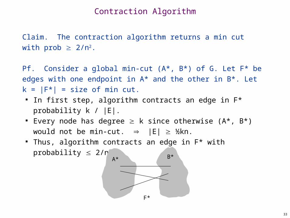
Claim. The contraction algorithm returns a min cut with prob 2/n2.
Pf. Consider a global min-cut (A*, B*) of G. Let F* be edges with one endpoint in A* and the other in B*. Let k = |F*| = size of min cut.
In first step, algorithm contracts an edge in F* probability k / |E|.
Every node has degree k since otherwise (A*, B*) would not be min-cut. |E| ½kn.
Thus, algorithm contracts an edge in F* with probability 2/n.
A* B*
F*
34
Contraction Algorithm
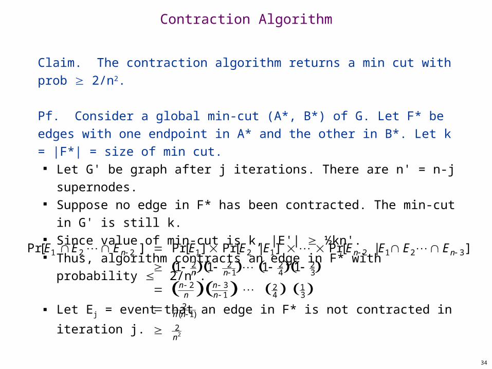
Claim. The contraction algorithm returns a min cut with prob 2/n2.
Pf. Consider a global min-cut (A*, B*) of G. Let F* be edges with one endpoint in A* and the other in B*. Let k = |F*| = size of min cut.
Let G' be graph after j iterations. There are n' = n-j supernodes. Suppose no edge in F* has been contracted. The min-cut in G' is
still k. Since value of min-cut is k, |E'| ½kn'. Thus, algorithm contracts an edge in F* with probability 2/n'.
Let Ej = event that an edge in F* is not contracted in iteration j.
Pr[E1 E2 En 2 ] Pr[E1] Pr[E2 | E1] Pr[En 2 | E1 E2 En 3]
1 2n 1 2
n1 1 24 1 2
3 n 2
n n 3n 1 2
4 13
2n(n1)
2n2
35
Contraction Algorithm
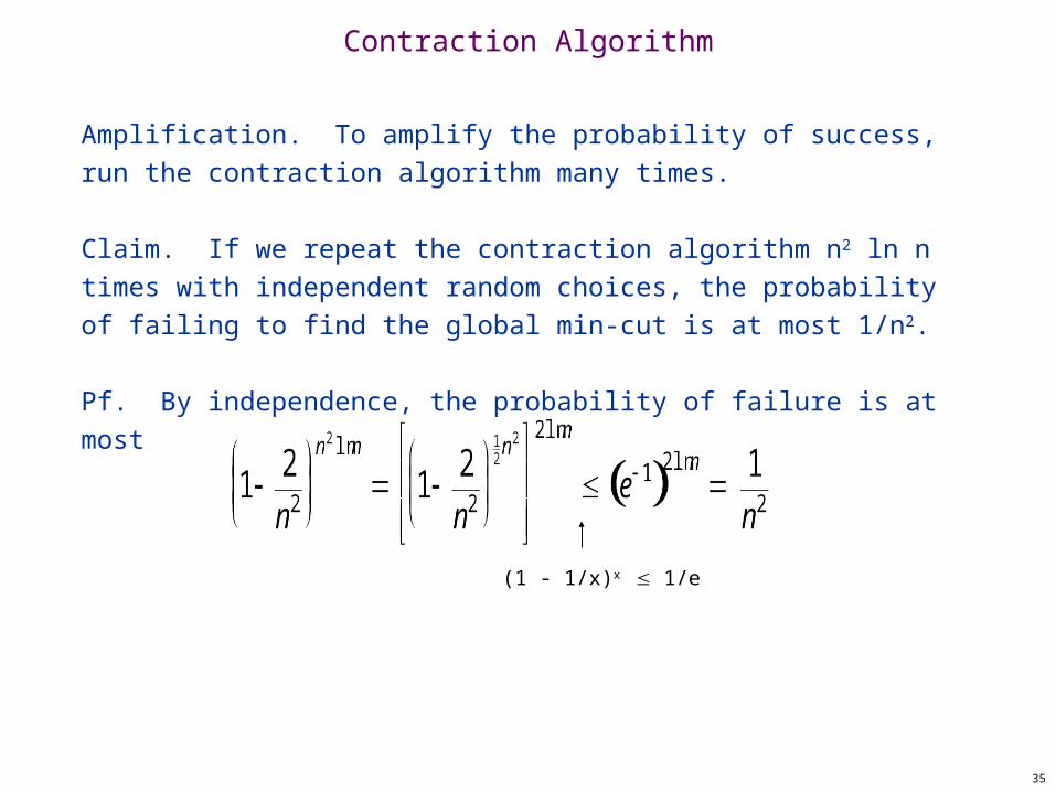
Amplification. To amplify the probability of success, run the contraction algorithm many times.
Claim. If we repeat the contraction algorithm n2 ln n times with independent random choices, the probability of failing to find the global min-cut is at most 1/n2.
Pf. By independence, the probability of failure is at most
(1 - 1/x)x 1/e
36
Global Min Cut: Context
Remark. Overall running time is slow since we perform (n2 log n) iterations and each takes (m) time.
Improvement. [Karger-Stein 1996] O(n2 log3n). Early iterations are less risky than later ones: probability of
contracting an edge in min cut hits 50% when n / √2 nodes remain.
Run contraction algorithm until n / √2 nodes remain. Run contraction algorithm twice on resulting graph, and return
best of two cuts.
Extensions. Naturally generalizes to handle positive weights.
Best known. [Karger 2000] O(m log3n).faster than best known max flow algorithm ordeterministic global min cut algorithm