Embed Size (px)
Citation preview
Seismic
Data
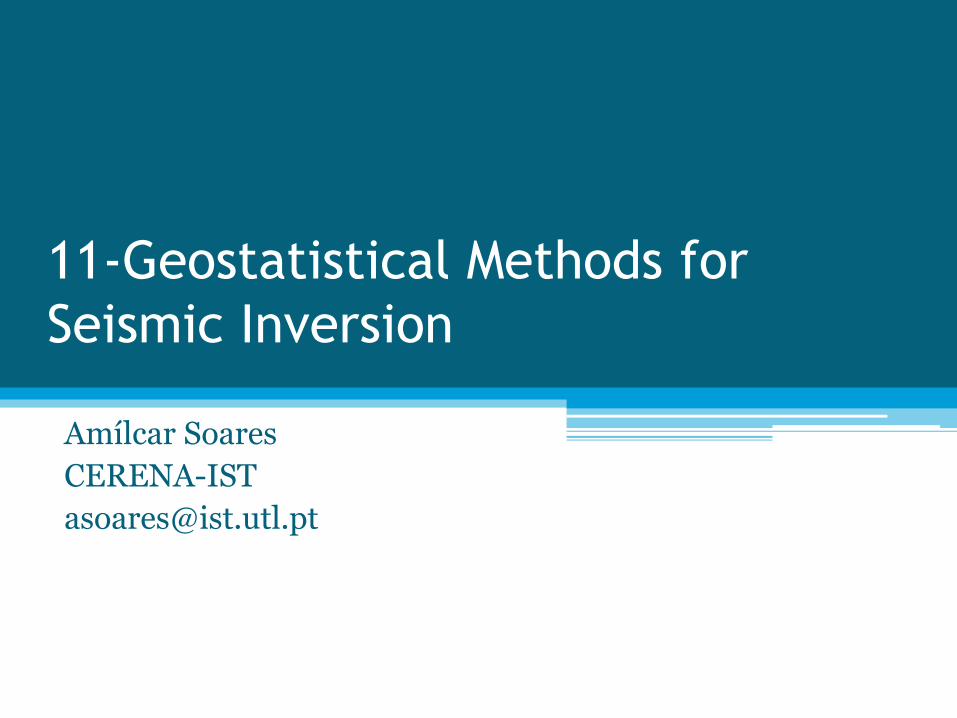
Seismic and Log Scale
01 - Introduction

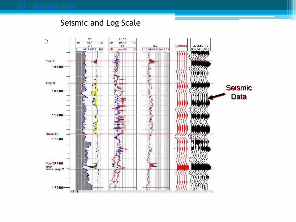
Velocity X Density = AI
Acoustic Impedance
Recap: basic concepts
Incident wave
Transmitted wave
Reflected wave Layer 1 impedance
= Velocity(1) x Density(1)
= Z1
Layer 2 impedance
= Velocity(2) x Density(2)
= Z2
Acoustic Impedance = Velocity X Density
Recap: basic concepts
“Since reflections are caused by changes in velocity and density, these two parameters are
combined into a parameter called “impedance”. This is the product of velocity and density “

Incident wave
Transmitted wave
Reflected wave
R = Reflected wavelet amplitude
Incident wavelet amplitude
R = Z2 - Z1
Z2 + Z1
R = (V2 x D2) - (V1 x D1)
(V2 x D2) + (V1 x D1)
Reflection coefficient
Recap: basic concepts
“ The ratio of the incident amplitude to the reflected amplitude is called the “Reflection Coefficient” .
Reflection coefficient can be seen a measure of the impedance contrast at the interface.”
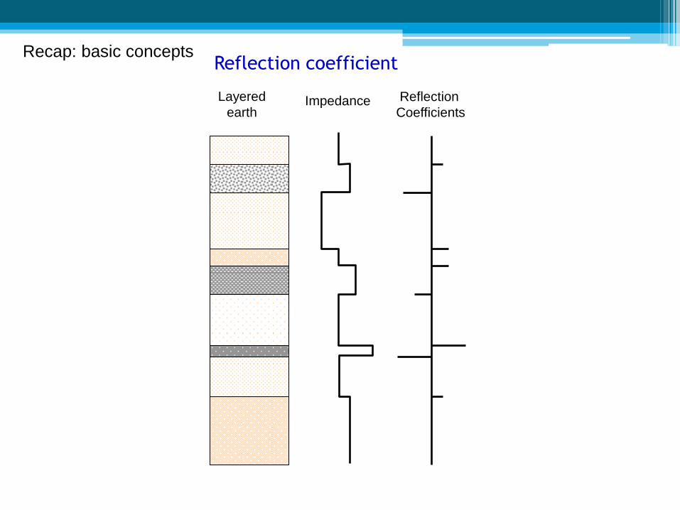
Layered
earth
Reflection
Coefficients Impedance
Reflection coefficient Recap: basic concepts
Marine air gun Land dynamite
Time
C - 2
Wavelet Recap: basic concepts
“A wavelet is a wave-like oscillation with an amplitude that starts out at
zero, increases, and then decreases back to zero.”
Time (Sec.)
Time origin
Zero phase
Minimum phase
Wavelet Recap: basic concepts

Lithology Impedance Minimum
phase
Zero
phase
Low
velocity
density
High
velocity
density
Recap: basic concepts Wavelet
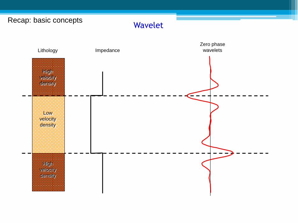
Lithology Impedance
Zero phase
wavelets
High
velocity
density
High
velocity
density
Low
velocity
density
Wavelet Recap: basic concepts

Incident wave
Transmitted wave
Reflected wave Layer 1 impedance
= Velocity(1) x Density(1)
= Z1
Layer 2 impedance
= Velocity(2) x Density(2)
= Z2
Impedance = Velocity X Density
02 – Seismic Inversion
Convolution
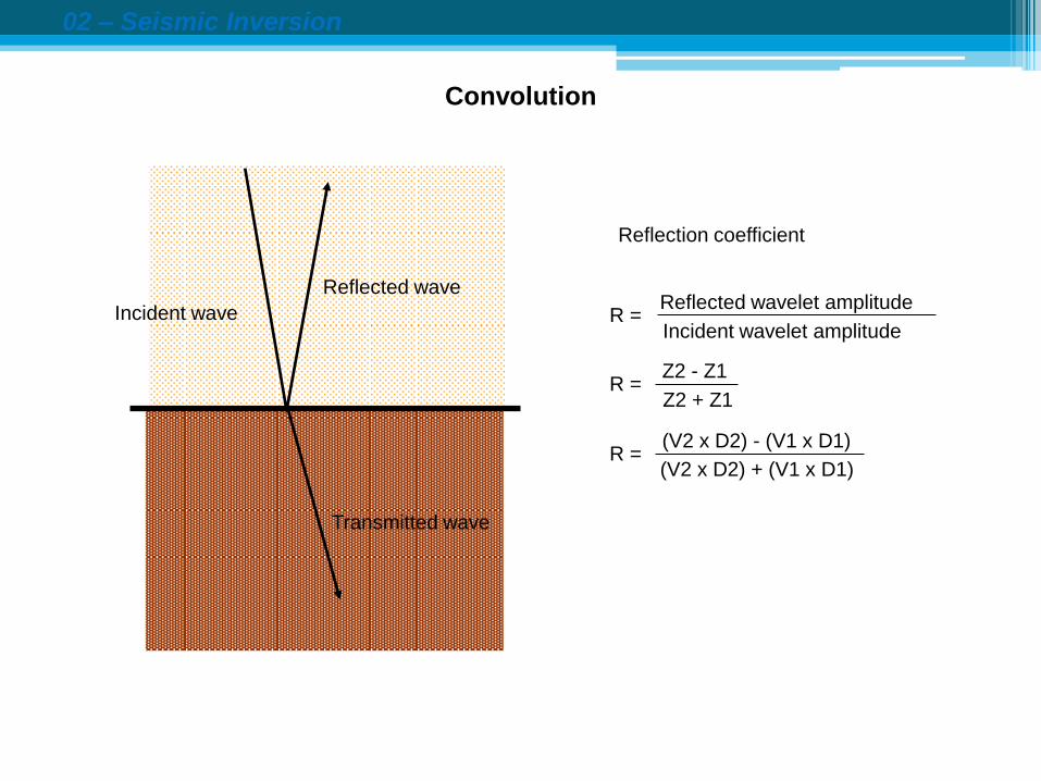
Incident wave
Transmitted wave
Reflected wave
Reflection coefficient
R = Reflected wavelet amplitude
Incident wavelet amplitude
R = Z2 - Z1
Z2 + Z1
R = (V2 x D2) - (V1 x D1)
(V2 x D2) + (V1 x D1)
02 – Seismic Inversion
Convolution
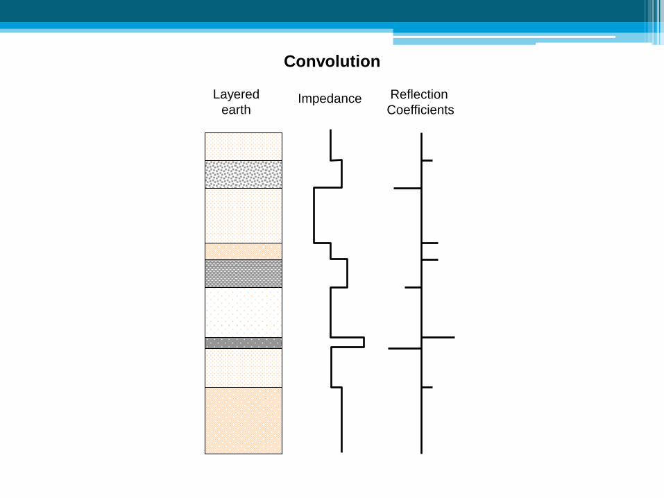
Layered
earth
Reflection
Coefficients Impedance
Convolution

Convolving the reflectivity coefficients c(x) with a
given wavelet w, one obtain the synthetic seismic
amplitudes a*(x)= c(x)*w
Principle of Seismic Inversion

Earth
Convolution - Forward exercise

Earth Impedance
Convolution - Forward exercise

Earth Reflection
Coefficients Impedance
Convolution - Forward exercise
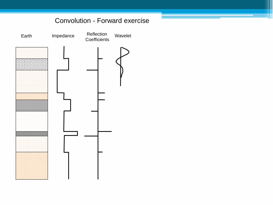
Earth Reflection
Coefficients Wavelet Impedance
Convolution - Forward exercise
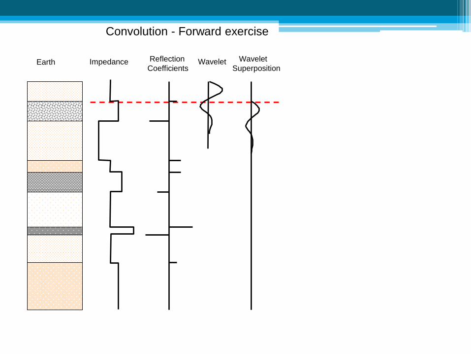
Earth Reflection
Coefficients Wavelet Wavelet
Superposition Impedance
Convolution - Forward exercise
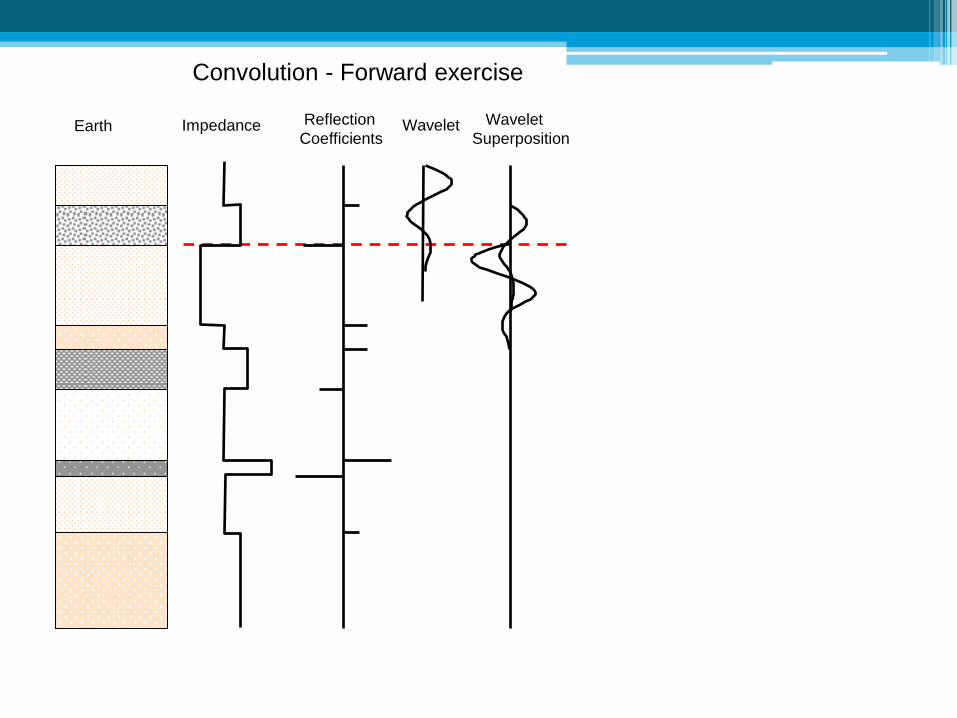
Earth Reflection
Coefficients Wavelet Wavelet
Superposition Impedance
Convolution - Forward exercise

Earth Reflection
Coefficients Wavelet Wavelet
Superposition Impedance
Convolution - Forward exercise
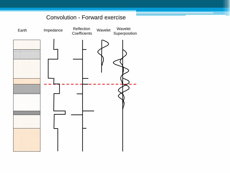
Earth Reflection
Coefficients Wavelet Wavelet
Superposition Impedance
Convolution - Forward exercise
Earth Reflection
Coefficients Wavelet Wavelet
Superposition Impedance
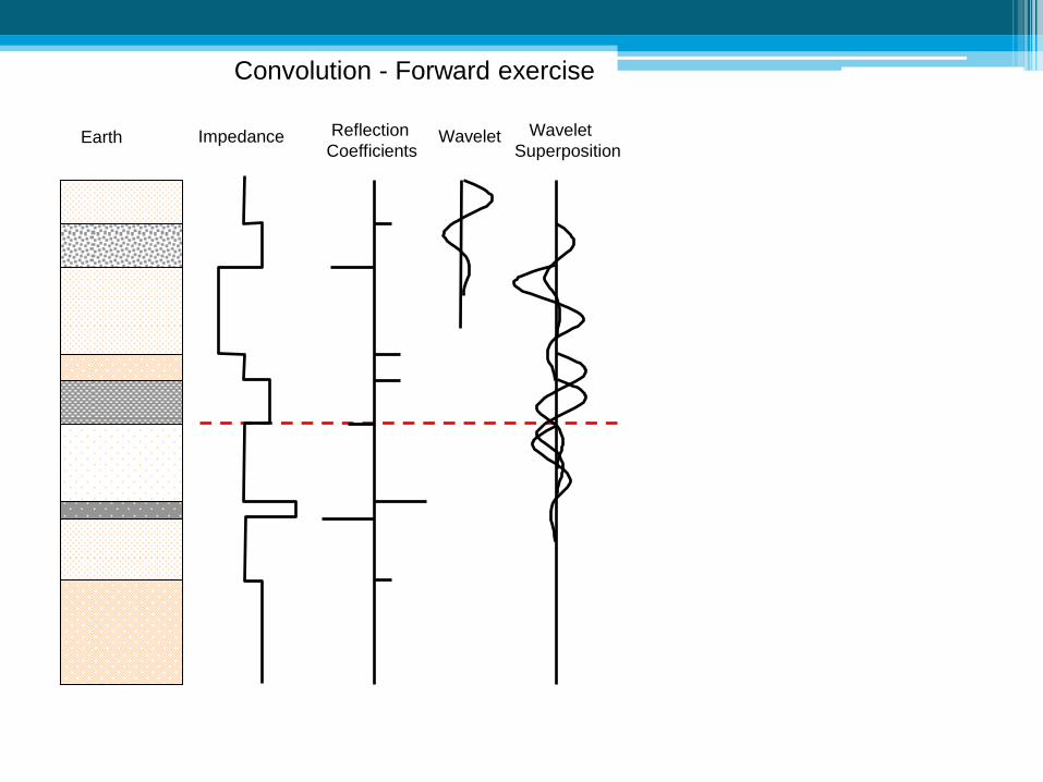
Convolution - Forward exercise
Earth Reflection
Coefficients Wavelet Wavelet
Superposition Impedance
Convolution - Forward exercise
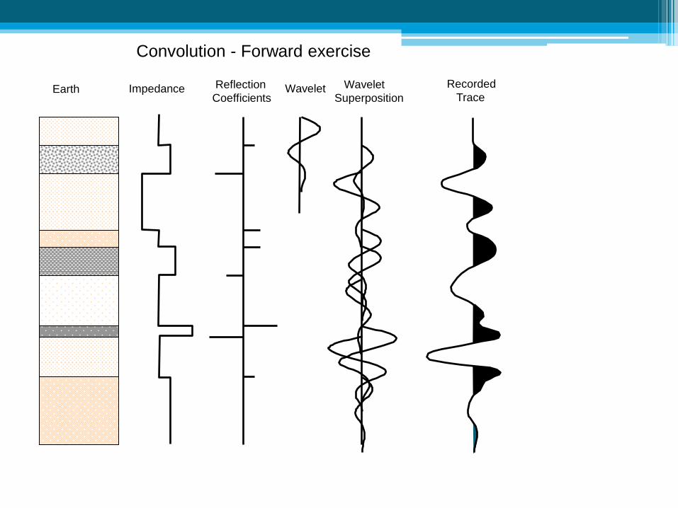
Earth Reflection
Coefficients Wavelet Wavelet
Superposition
Recorded
Trace Impedance
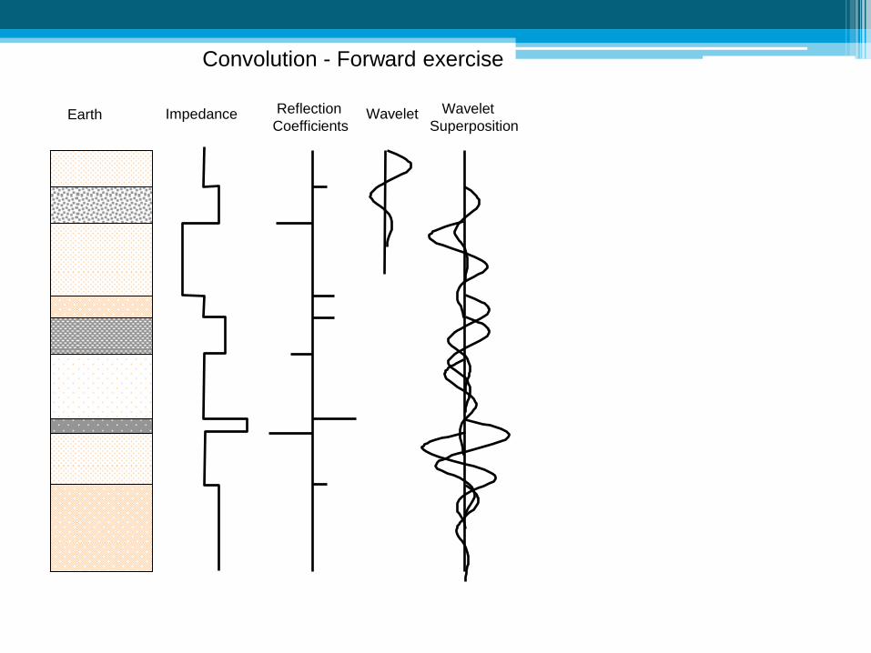
Convolution - Forward exercise
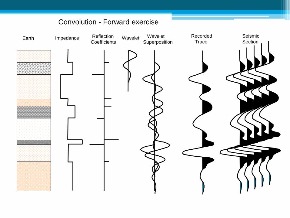
Earth Reflection
Coefficients Wavelet Wavelet
Superposition
Recorded
Trace
Seismic
Section Impedance
Convolution - Forward exercise

Seismic
Section
Convolution - Inverse Exercise

Recorded
Trace Seismic
Section
Convolution - Inverse Exercise
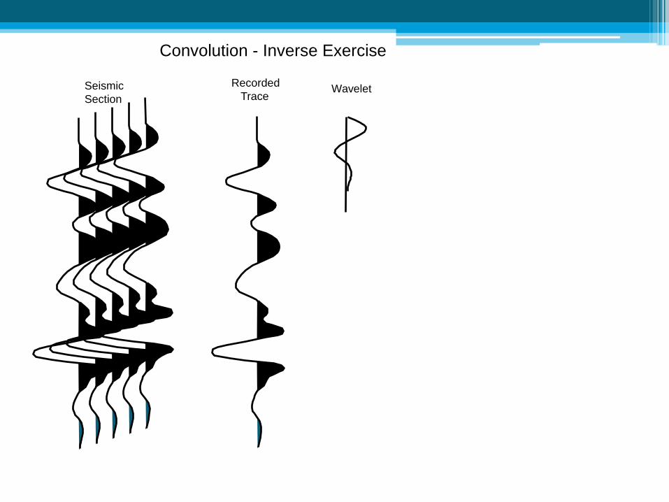
Wavelet Recorded
Trace Seismic
Section
Convolution - Inverse Exercise
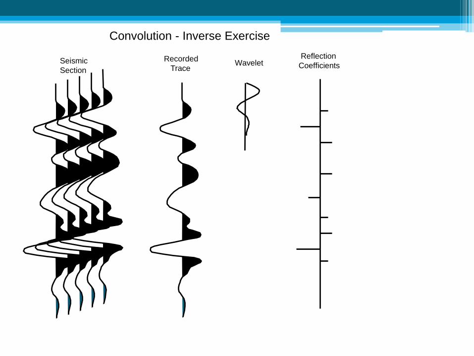
Reflection
Coefficients Wavelet Recorded
Trace Seismic
Section
Convolution - Inverse Exercise

Reflection
Coefficients Wavelet Recorded
Trace Seismic
Section
Reflection
Coefficients
Convolution - Inverse Exercise
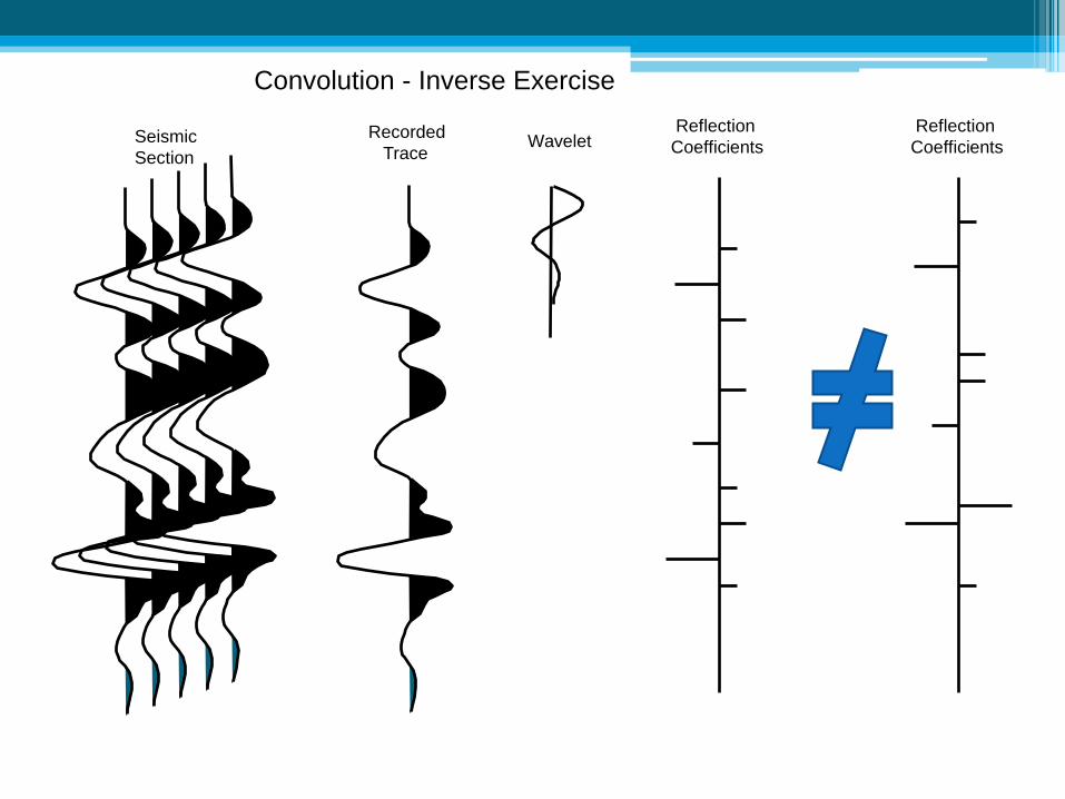
Reflection
Coefficients Wavelet Recorded
Trace Seismic
Section
Reflection
Coefficients
Convolution - Inverse Exercise
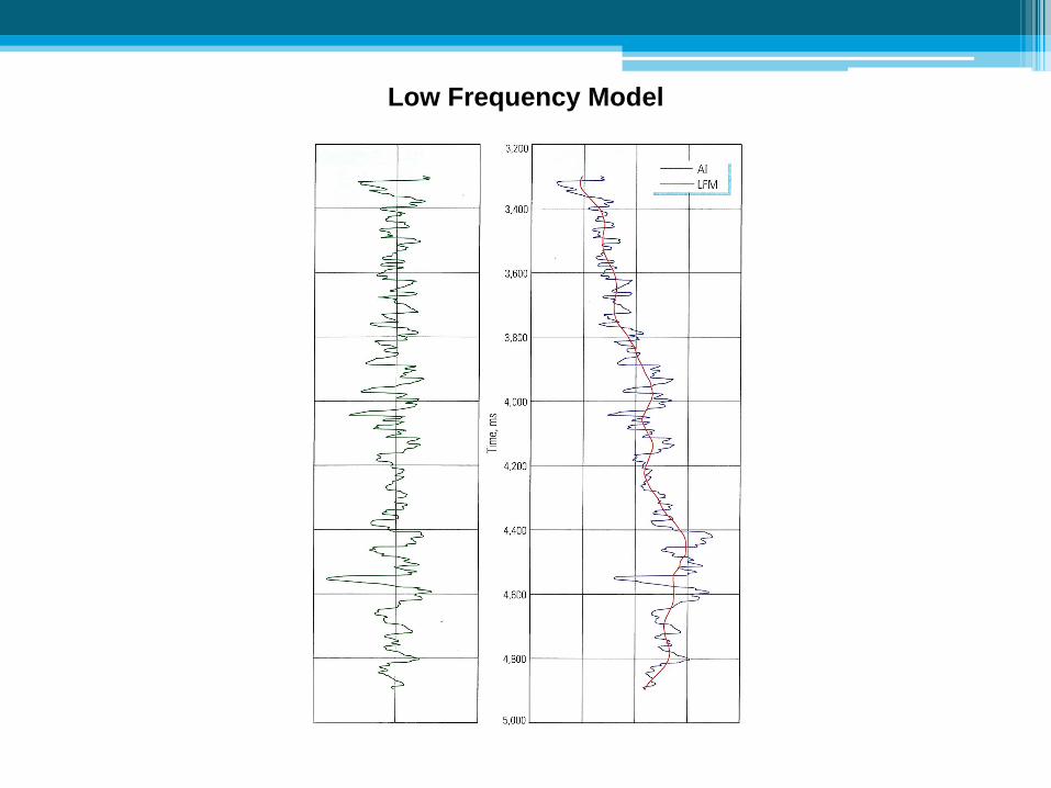
Low Frequency Model

• Inverse Modeling is based on the physical relation:
-1000.0000
-500.0000
0.0000
500.0000
1000.0000
1500.0000
-20 -15 -10 -5 0 5 10 15 20
ms
am
pli
tud
e
* =
Convolving the reflectivity coefficients c(x) with a
given wavelet w, one obtain the synthetic seismic
amplitudes a*(x)= c(x)*w
Typical Inverse Problem: one whish to know the acoustic impedances which
give rise to the known real seismic.

Typical Inverse Problem: one wish calculate the parameters ( high
resolution grid of acoustic impedance) that give rise to the solution we
know (the real seismic)
In this problem there is not a unique solution. One whish to find the set of
solutions that accomplish the spatial requisites of the acoustic impedance
grid: spatial continuity pattern, global CDfs, ...
Outline of the iterative method
Space of the
Parameters
Solution for
the set of
parameters
Compare with the
known real solution
Is the match
satisfactory ?
N
Change the set of
parameters in order to
make the process
convergent

Geostatistical Seismic Inversion
The aim of geostatistical inversion of seismic is to produce high
resolution of numerical models that have two properties:
•The numerical model honors a physical relationship (convolution model)
with the actual data .
•The numerical model reflects the spatial continuity and the global
distribution functions .
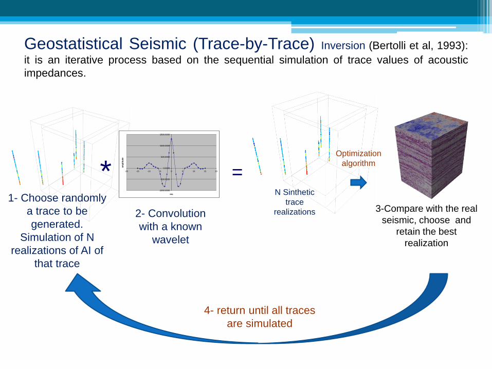
Geostatistical Seismic (Trace-by-Trace) Inversion (Bertolli et al, 1993):
it is an iterative process based on the sequential simulation of trace values of acoustic
impedances.
-1000.0000
-500.0000
0.0000
500.0000
1000.0000
1500.0000
-20 -15 -10 -5 0 5 10 15 20
ms
am
pli
tud
e
* =
1- Choose randomly
a trace to be
generated.
Simulation of N
realizations of AI of
that trace
N Sinthetic
trace
realizations 3-Compare with the real
seismic, choose and
retain the best
realization
4- return until all traces
are simulated
Optimization
algorithm
2- Convolution
with a known
wavelet
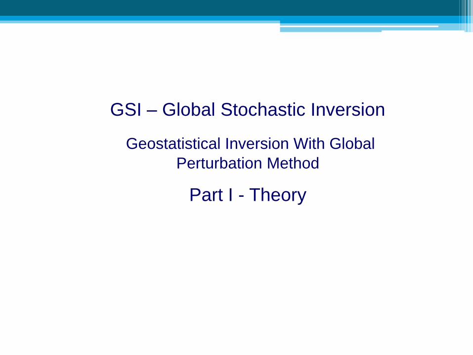
GSI – Global Stochastic Inversion
Geostatistical Inversion With Global
Perturbation Method
Part I - Theory
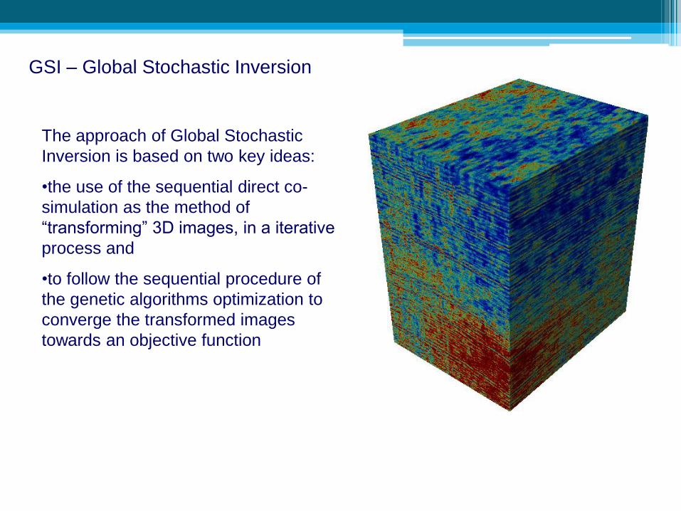
The approach of Global Stochastic
Inversion is based on two key ideas:
•the use of the sequential direct co-
simulation as the method of
“transforming” 3D images, in a iterative
process and
•to follow the sequential procedure of
the genetic algorithms optimization to
converge the transformed images
towards an objective function
GSI – Global Stochastic Inversion

2- Convolution of transformed Simulated
Acoustic Impedance
-1000.0000
-500.0000
0.0000
500.0000
1000.0000
1500.0000
-20 -15 -10 -5 0 5 10 15 20
ms
am
pli
tud
e
*
1 – Simulation of Acoustic
Impedance

3 – Comparing the synthetic amplitudes a*(x)
with the real seismic a(x) obtaining local
correlation coefficients cc(x)
5 – Return to step one to obtain a new
generation of AI images until a given objective
function is reached.
4 – From the N realizations, retain the traces
with best matches and “compose” a best
image of AI
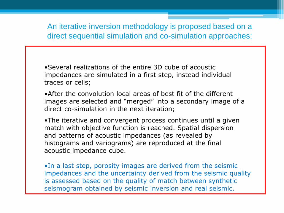
An iterative inversion methodology is proposed based on a
direct sequential simulation and co-simulation approaches:
•Several realizations of the entire 3D cube of acoustic impedances are simulated in a first step, instead individual traces or cells;
•After the convolution local areas of best fit of the different images are selected and “merged” into a secondary image of a direct co-simulation in the next iteration;
•The iterative and convergent process continues until a given match with objective function is reached. Spatial dispersion and patterns of acoustic impedances (as revealed by histograms and variograms) are reproduced at the final acoustic impedance cube.
•In a last step, porosity images are derived from the seismic impedances and the uncertainty derived from the seismic quality is assessed based on the quality of match between synthetic seismogram obtained by seismic inversion and real seismic.
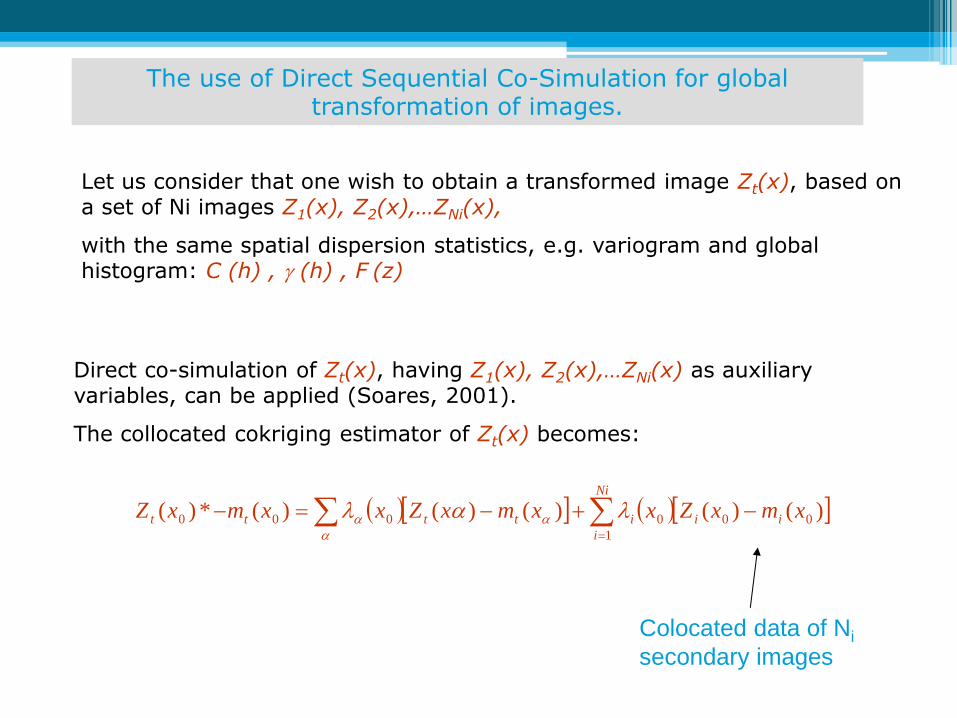
The use of Direct Sequential Co-Simulation for global transformation of images.
Let us consider that one wish to obtain a transformed image Zt(x), based on a set of Ni images Z1(x), Z2(x),…ZNi(x),
with the same spatial dispersion statistics, e.g. variogram and global histogram: C (h) , (h) , F (z)
Direct co-simulation of Zt(x), having Z1(x), Z2(x),…ZNi(x) as auxiliary variables, can be applied (Soares, 2001).
The collocated cokriging estimator of Zt(x) becomes:
)()()()()(*)( 00
1
0000 xmxZxxmxZxxmxZ ii
Ni
i
itttt
Colocated data of Ni
secondary images

Variable Z1(x)
3 realizations from variable Z2(x)
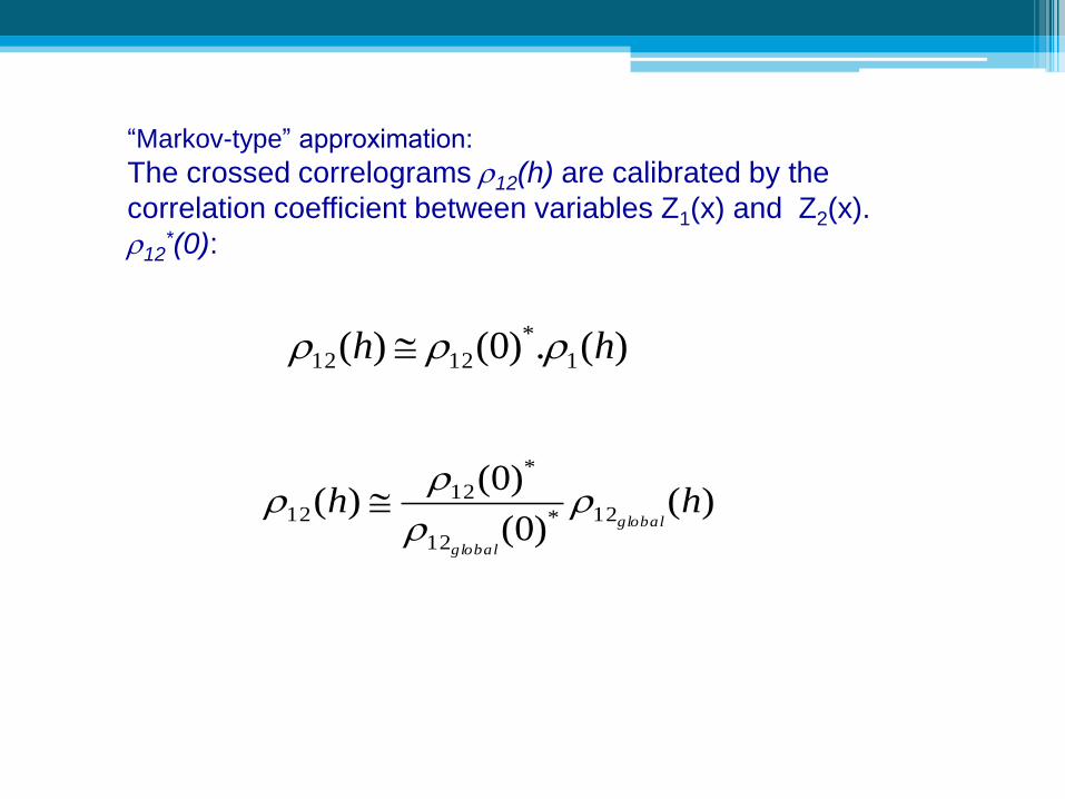
“Markov-type” approximation:
The crossed correlograms 12(h) are calibrated by the
correlation coefficient between variables Z1(x) and Z2(x).
12*(0):
)(.)0()( 1
*
1212 hh
)()0(
)0()( 12*
12
*
1212 hh
global
global

=.95 =.80 =.60
Variable Z1(x)
Simulation of variable Z2(x)
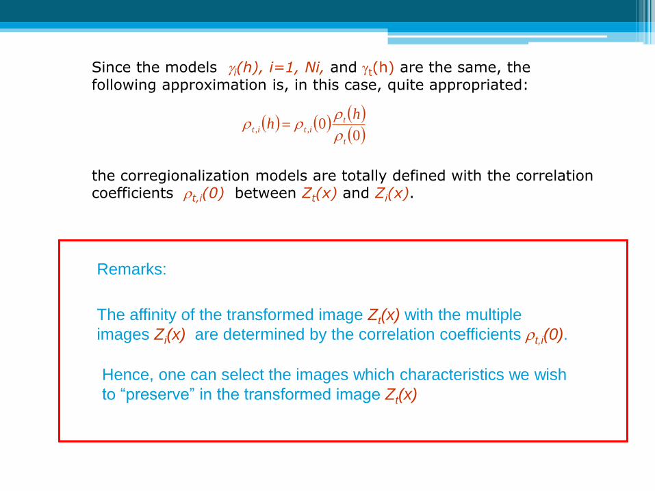
Since the models i(h), i=1, Ni, and t(h) are the same, the following approximation is, in this case, quite appropriated:
The affinity of the transformed image Zt(x) with the multiple
images Zi(x) are determined by the correlation coefficients t,i(0).
Hence, one can select the images which characteristics we wish
to “preserve” in the transformed image Zt(x)
Remarks:
0
0,,
t
titit
hh
the corregionalization models are totally defined with the correlation coefficients t,i(0) between Zt(x) and Zi(x).
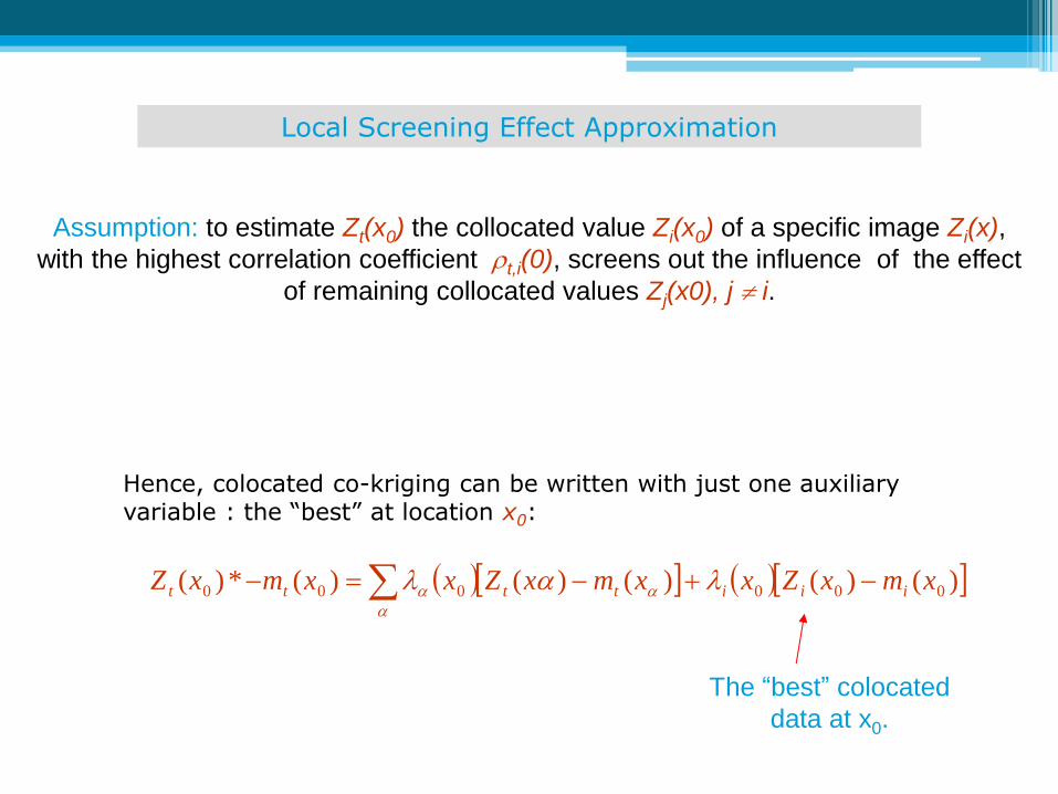
Local Screening Effect Approximation
Assumption: to estimate Zt(x0) the collocated value Zi(x0) of a specific image Zi(x),
with the highest correlation coefficient t,i(0), screens out the influence of the effect
of remaining collocated values Zj(x0), j i.
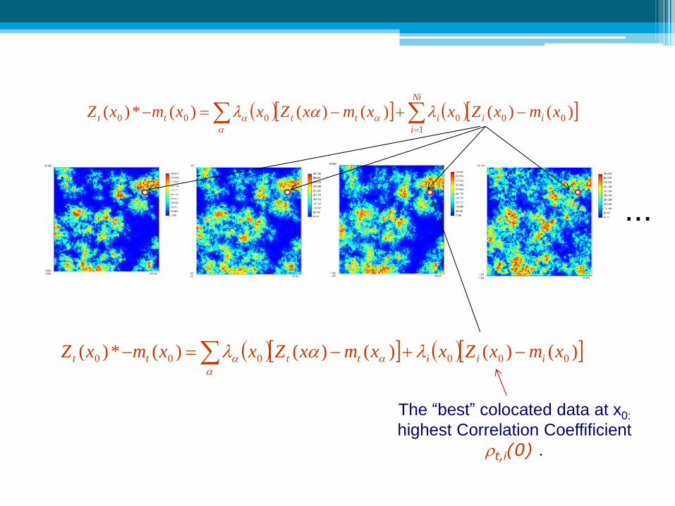
Hence, colocated co-kriging can be written with just one auxiliary variable : the “best” at location x0:
)()()()()(*)( 000000 xmxZxxmxZxxmxZ iiitttt
The “best” colocated
data at x0.
)()()()()(*)( 00
1
0000 xmxZxxmxZxxmxZ ii
Ni
i
itttt
...
)()()()()(*)( 000000 xmxZxxmxZxxmxZ iiitttt
The “best” colocated data at x0:
highest Correlation Coeffificient
t,i(0) .

Outline of the proposed methodology
GSI – Global Stochastic Inversion
i- Generate a set of initial images of acoustic impedances by using direct sequential simulation.
ii- Create the synthetic seismogram of amplitudes, by
convolving the reflectivity, derived from acoustic impedances, with a known wavelet.
iii- Evaluate the match of the synthetic seismograms, of entire
3D image, and the real seismic by computing, for example local correlation coefficients.
iv - Ranking the “best” images based on the match (e.g. the average value or a percentile of correlation coefficients for the entire image). From them, one select the best parts- the columns or the horizons with the best correlation coefficient – of each image. Compose one auxiliary image with the selected “best” parts, for the next simulation step. v- Generate a new set of images, by direct co-simulation, and return to step ii) until a given threshold of the objective function is reached.

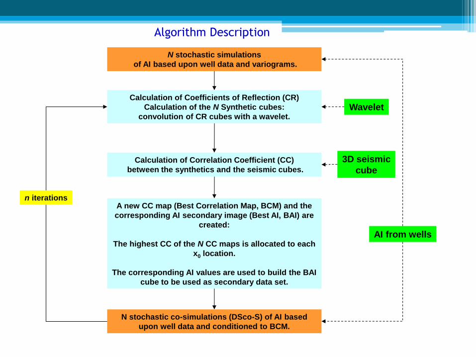
AI from wells
N stochastic simulations
of AI based upon well data and variograms.
Calculation of Coefficients of Reflection (CR)
Calculation of the N Synthetic cubes:
convolution of CR cubes with a wavelet.
Calculation of Correlation Coefficient (CC)
between the synthetics and the seismic cubes.
A new CC map (Best Correlation Map, BCM) and the
corresponding AI secondary image (Best AI, BAI) are
created:
The highest CC of the N CC maps is allocated to each
x0 location.
The corresponding AI values are used to build the BAI
cube to be used as secondary data set.
N stochastic co-simulations (DSco-S) of AI based
upon well data and conditioned to BCM.
3D seismic
cube
n iterations
Wavelet
03 – Algorithm Description
Algorithm Description
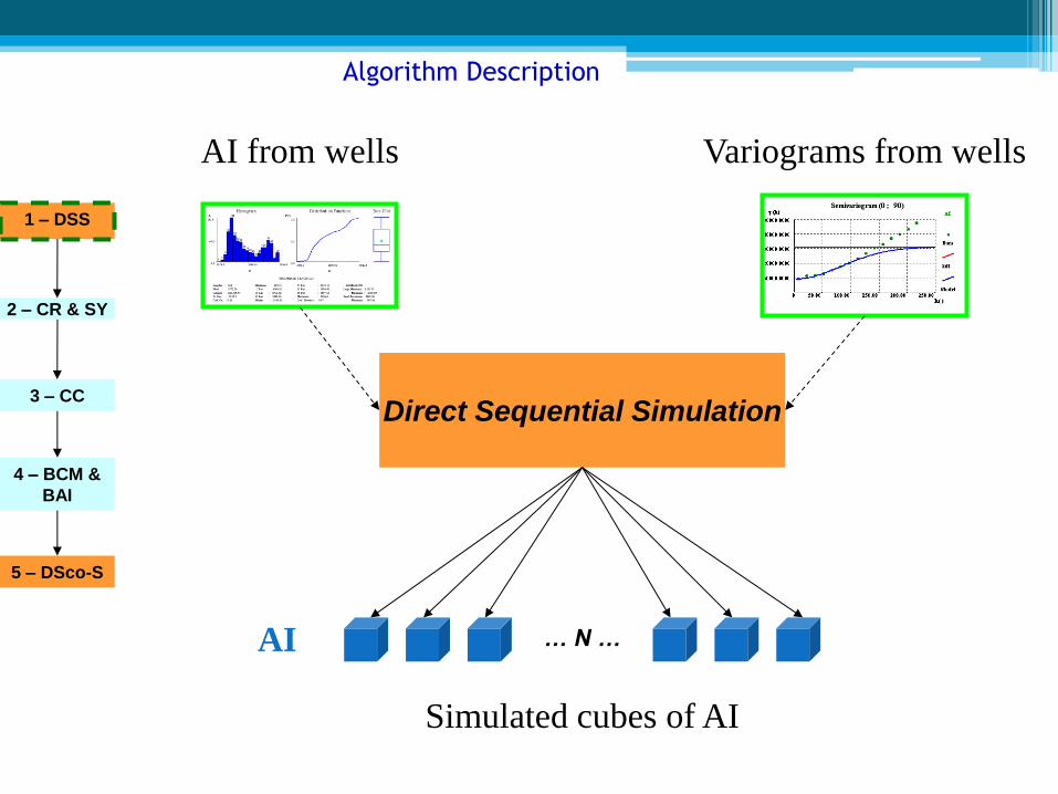
Direct Sequential Simulation
1 – DSS
2 – CR & SY
3 – CC
4 – BCM &
BAI
5 – DSco-S
AI from wells Variograms from wells
… N …
Simulated cubes of AI
AI
Algorithm Description

1 – DSS
2 – CR
& SY
3 – CC
4 – BCM
& BAI
5 – DSco-S
… N …
)()1(
)()1()(
tAitAi
tAitAitCr
AI
-40000
-20000
0
20000
40000
60000
80000
100000
120000
-135 -117 -99 -81 -63 -45 -27 -9 9 27 45 63 81 99 117 135
Wavelet
… N … SY
Synthetic cubes
… N … CR Coefficient of
Reflection cubes
)()()( zwavetCrtSy Convolution
Algorithm Description
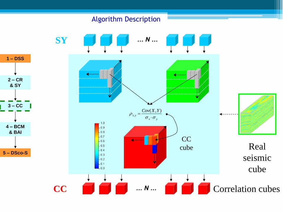
1 – DSS
2 – CR
& SY
3 – CC
5 – DSco-S
… N … SY
yx
yx
YXCov
),(,
Real
seismic
cube
CC
cube
… N … CC Correlation cubes
4 – BCM
& BAI
Algorithm Description
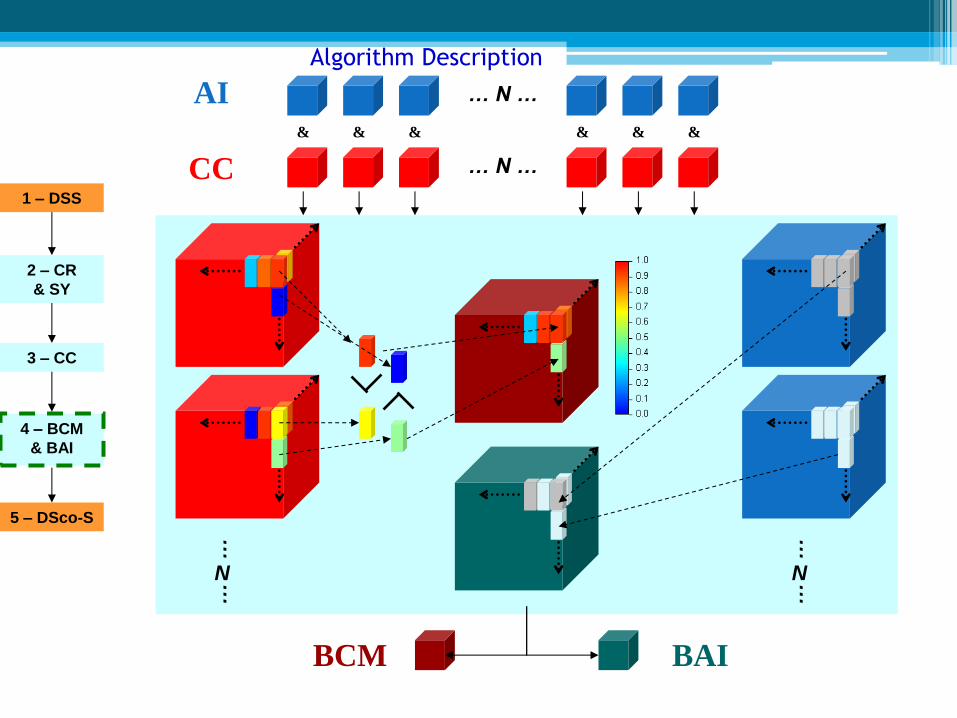
… …
N
… …
N
4 – BCM
& BAI
1 – DSS
2 – CR
& SY
3 – CC
5 – DSco-S
… N … CC
… N … AI & & & & & &
BCM BAI
Algorithm Description
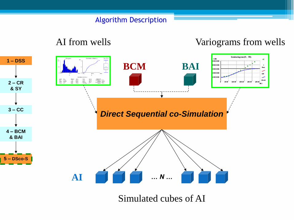
Direct Sequential co-Simulation
1 – DSS
2 – CR
& SY
3 – CC
4 – BCM
& BAI
5 – DSco-S
AI from wells Variograms from wells
… N …
Simulated cubes of AI
AI
BCM BAI
Algorithm Description
AI from wells
N stochastic simulations
of AI based upon well data and variograms.
Calculation of Coefficients of Reflection (CR)
Calculation of the N Synthetic cubes:
convolution of CR cubes with a wavelet.
Calculation of Correlation Coefficient (CC)
between the synthetics and the seismic cubes.
A new CC map (Best Correlation Map, BCM) and the
corresponding AI secondary image (Best AI, BAI) are
created:
The highest CC of the N CC maps is allocated to each
x0 location.
The corresponding AI values are used to build the BAI
cube to be used as secondary data set.
N stochastic co-simulations (DSco-S) of AI based
upon well data and conditioned to BCM.
3D seismic
cube
n iterations
Wavelet
Algorithm Description
04 – Results
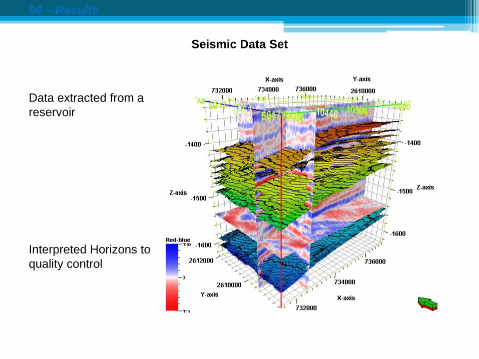
Seismic Data Set
Data extracted from a
reservoir
Interpreted Horizons to
quality control
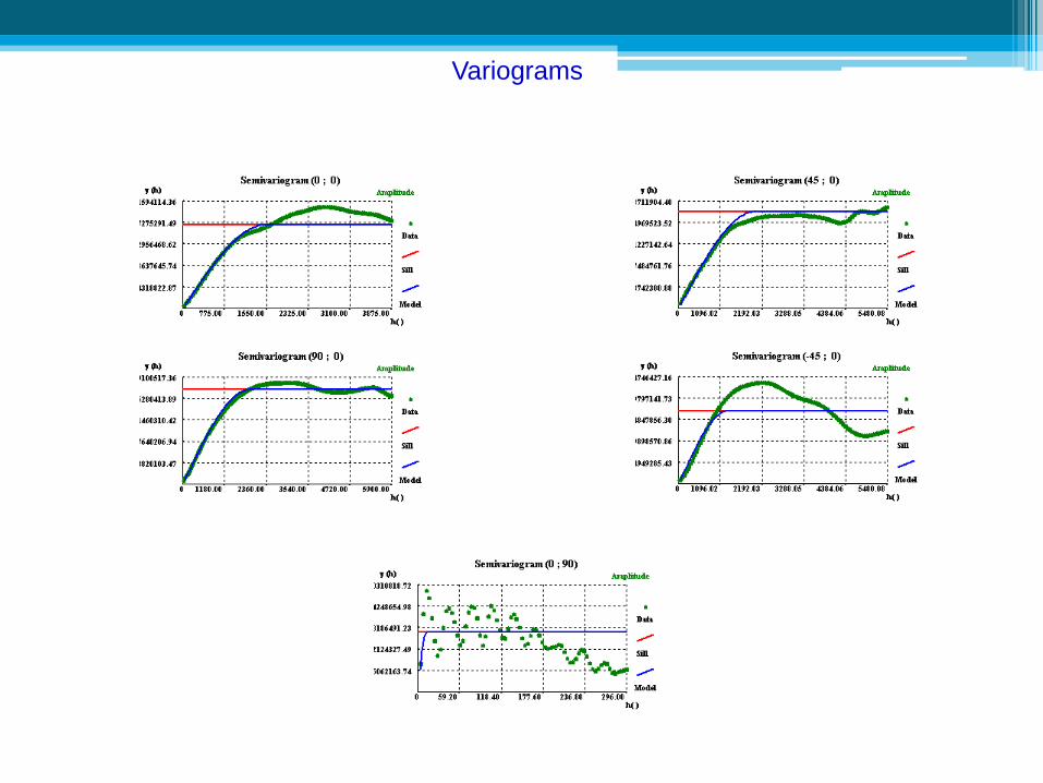
Variograms
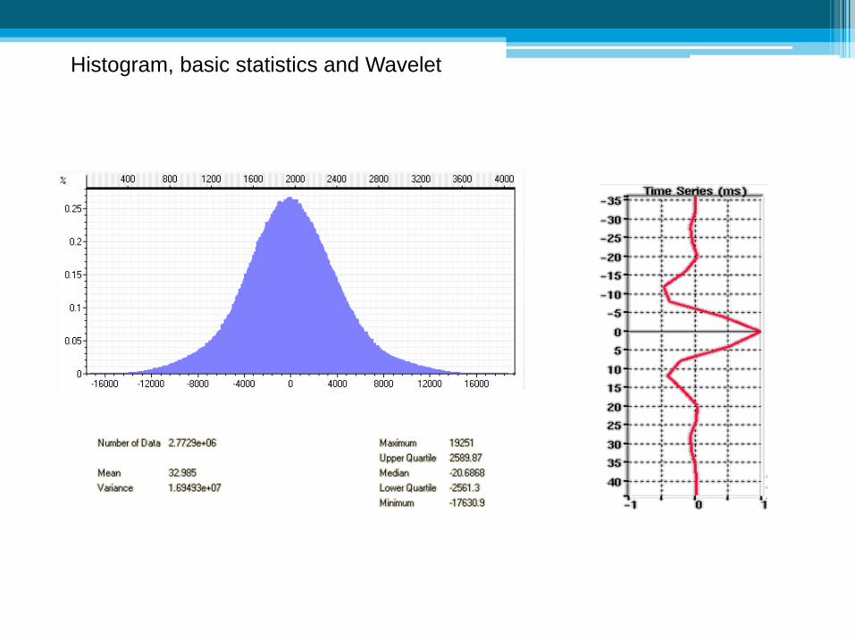
Histogram, basic statistics and Wavelet
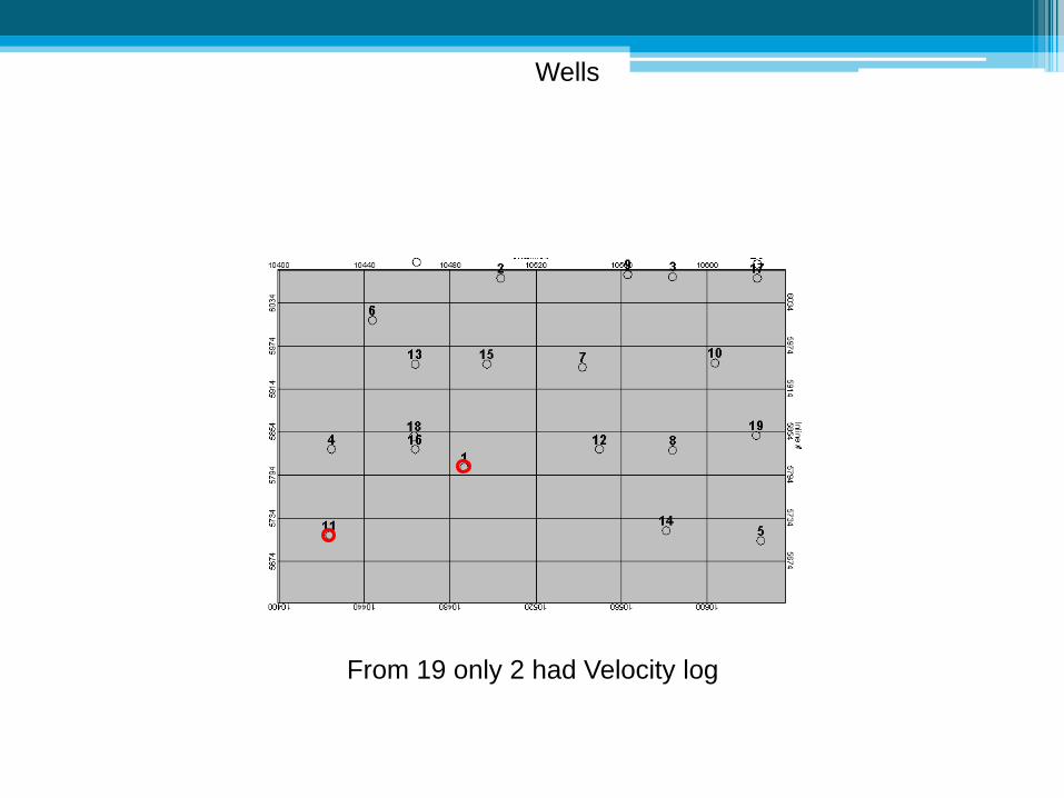
Wells
From 19 only 2 had Velocity log
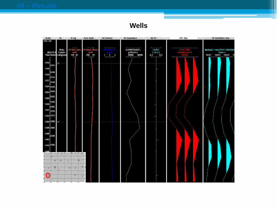
04 – Results
Wells
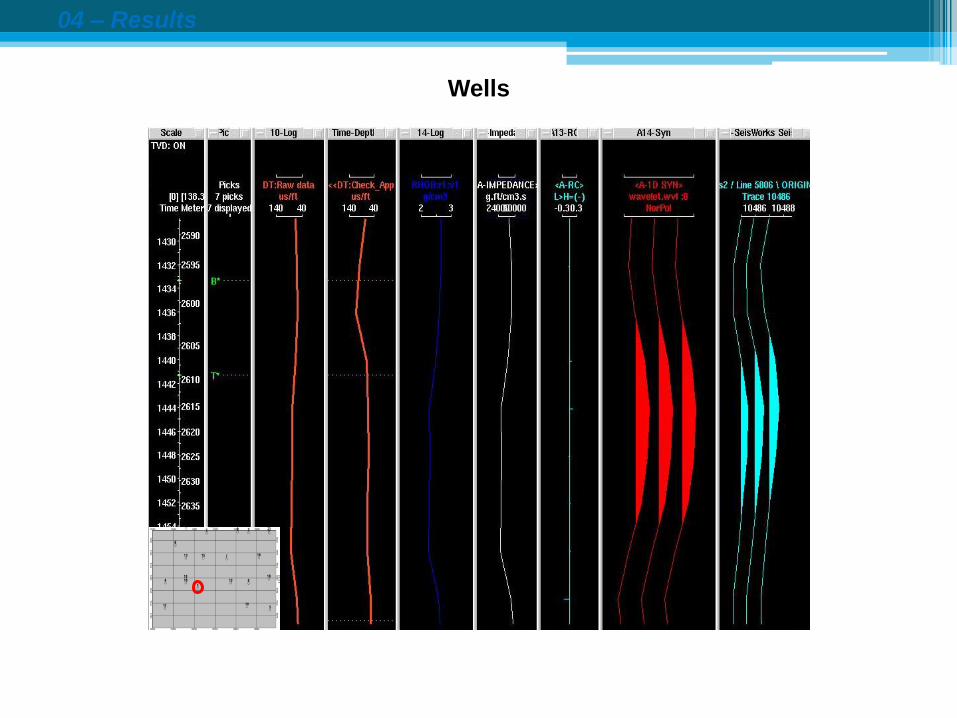
04 – Results
Wells
04 – Results
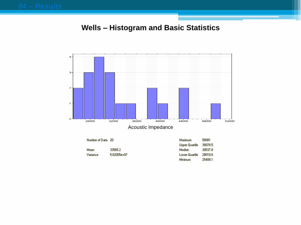
Wells – Histogram and Basic Statistics
Acoustic Impedance

04 – Results
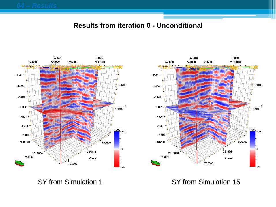
Results from iteration 0 - Unconditional
AI from Simulation 1 AI from Simulation 15
04 – Results
Results from iteration 0 - Unconditional
SY from Simulation 1 SY from Simulation 15

04 – Results
Results from iteration 0 - Unconditional
CC from Simulation 1 CC from Simulation 15
04 – Results
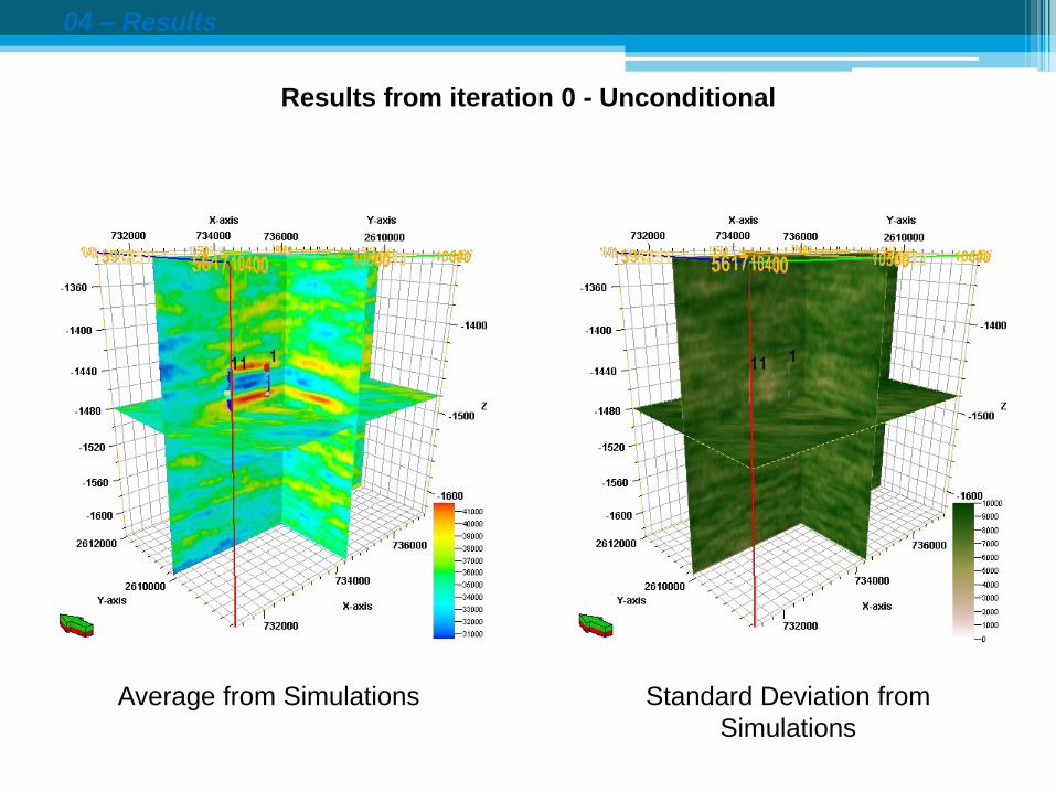
Results from iteration 0 - Unconditional
Average from Simulations Standard Deviation from
Simulations
04 – Results
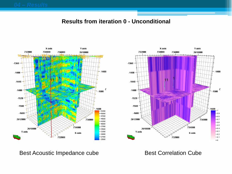
Results from iteration 0 - Unconditional
Best Acoustic Impedance cube Best Correlation Cube

04 – Results
Results from Process
0.85 0.87 0.88
0.80
0.62
0.080
0.1
0.2
0.3
0.4
0.5
0.6
0.7
0.8
0.9
1
0 1 2 3 4 5
Iterations
Co
rre
lati
on
04 – Results
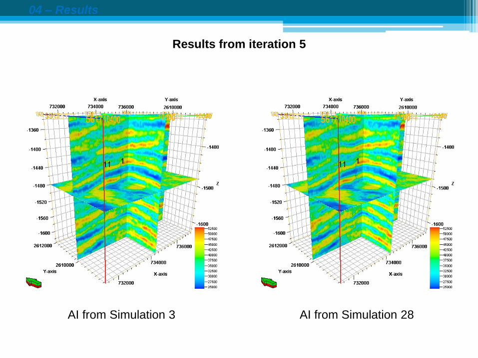
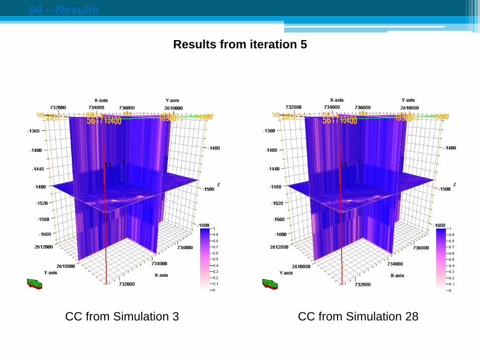
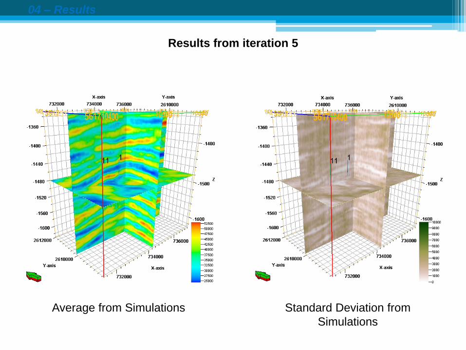
Results from iteration 5
AI from Simulation 3 AI from Simulation 28

04 – Results
Results from iteration 5
SY from Simulation 3 SY from Simulation 28
04 – Results
Results from iteration 5
CC from Simulation 3 CC from Simulation 28
04 – Results
Results from iteration 5
Average from Simulations Standard Deviation from
Simulations
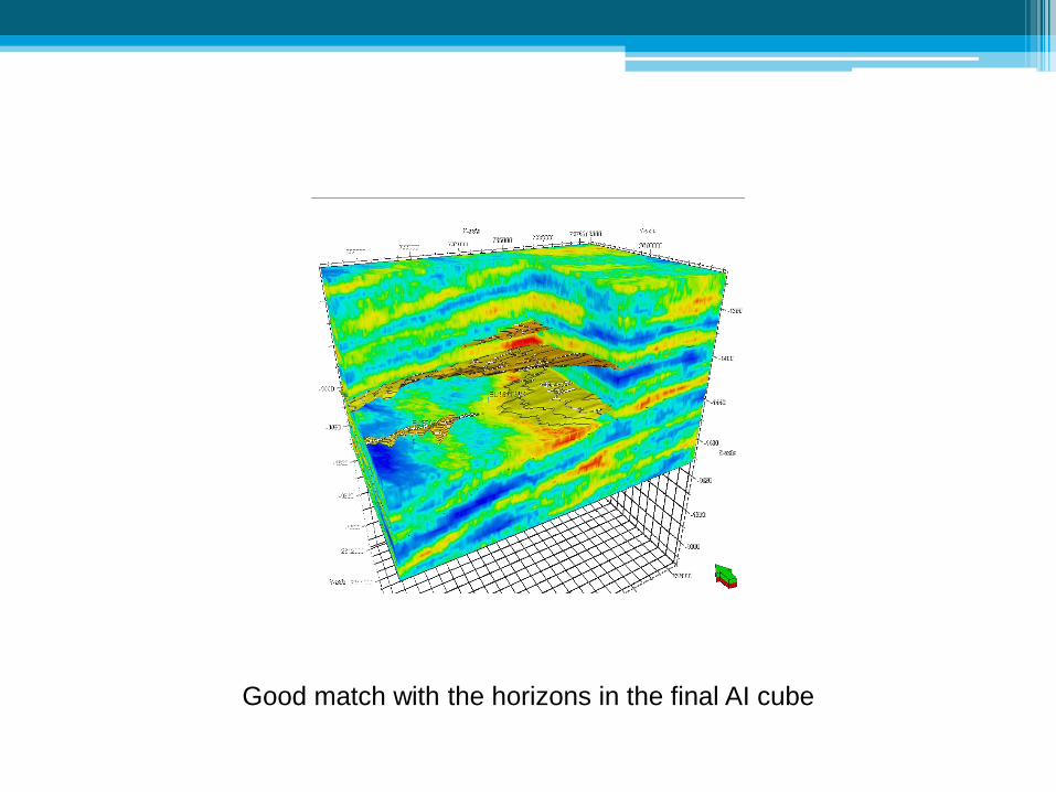
Good match with the horizons in the final AI cube
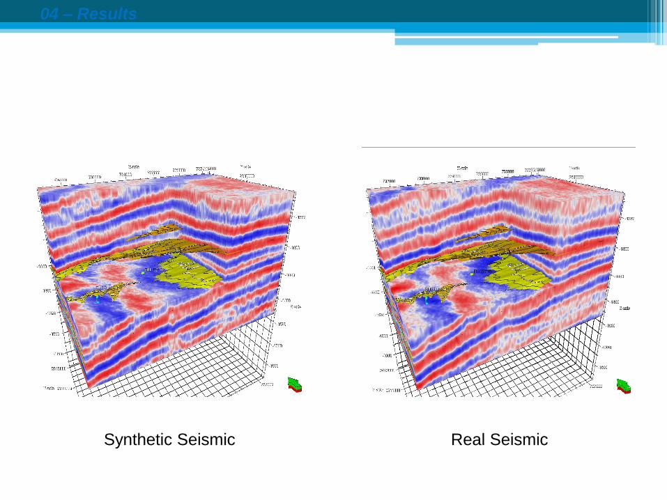
04 – Results
Synthetic Seismic Real Seismic
Practice VII- Seismic Inversion
Practice with GSI (Student) – Global Stochastic Inversion
Practice with S-GeMS – Stanford Geostatistical Modelling Software


![Joint AVO Inversion with Geostatistical Simulation · 2013-03-23 · Geostatistical Inversion (for example Pendrel et al., CSEG 2004, [1] and Van der Laan & Pendrel, SEG 2001 [2])](https://img.dokumen.tips/doc/110x75/5edab0f0ea30a273770f4bbc/joint-avo-inversion-with-geostatistical-simulation-2013-03-23-geostatistical-inversion.jpg)