Copyright 2000, Society of Petroleum Engineers Inc.

This paper was prepared for presentation at the 2000 SPE Annual Technical Conference andExhibition held in Dallas, Texas, 1–4 October 2000.

This paper was selected for presentation by an SPE Program Committee following review ofinformation contained in an abstract submitted by the author(s). Contents of the paper, aspresented, have not been reviewed by the Society of Petroleum Engineers and are subject tocorrection by the author(s). The material, as presented, does not necessarily reflect anyposition of the Society of Petroleum Engineers, its officers, or members. Papers presented atSPE meetings are subject to publication review by Editorial Committees of the Society ofPetroleum Engineers. Electronic reproduction, distribution, or storage of any part of this paperfor commercial purposes without the written consent of the Society of Petroleum Engineers isprohibited. Permission to reproduce in print is restricted to an abstract of not more than 300words; illustrations may not be copied. The abstract must contain conspicuousacknowledgment of where and by whom the paper was presented. Write Librarian, SPE, P.O.Box 833836, Richardson, TX 75083-3836, U.S.A., fax 01-972-952-9435.

AbstractInterpretation of well-log data into petrophysical variables,such as effective porosity, permeability, and effective fluidsaturation, provides an initial assessment of commercialhydrocarbon assets in the near vicinity of a well. A moreaccurate assessment requires quantitative indication of lateralcontinuity away from the well. Because wireline tools canonly sense rock formation properties a few meters away fromthe well, assessment of lateral continuity is at best donequalitatively with the aid of stratigraphic analysis or well-to-well correlations. Seldom do these extrapolation methods takeadvantage of the nowadays commonly available 3D seismicdata. In effect, despite possessing much less vertical resolutionthan well-log data, 3D seismic data have good lateralresolution that can naturally complement the verticalresolution of well-log data. We have developed an estimationprocedure whereby wireline data can be extrapolated awayfrom existing wells using geostatistical inversion of post-stack3D seismic data. This procedure works by estimating a jointprobability density function (PDF) that defines a physicalrelationship between seismic measurements (e.g. P-wavevelocity, and P-wave acoustic impedance), and petrophysicalvariables (e.g. density/porosity and bed thickness) rendered bywell-log data. The estimated joint PDF is further normalizedto reflect a vertical resolution midway between the resolutionof seismic data and the resolution of well-log data.Variograms are also estimated from well-log and seismic datathat define the expected degree of lateral smoothness awayfrom the well. We then generate stochastic realizations ofpetrophysical variables that not only honor the well-log data,

but most importantly, that fully honor the 3D seismic data in aleast-squares sense. In the presence of closely spaced wells,geostatistical inversion can also be used to estimate anaccurate static reservoir model for the subsequent simulationand planning of in-fill drilling and/or enhanced-oil-recoveryoperations. Examples are described in which geostatisticalinversion provides lateral delineations of sand units consistentwith measured fluid production data.

IntroductionPost-stack three-dimensional (3D) seismic data are mostcommonly used in the exploration world to delineategeological structures evidenced by continuous lateralreflection events. A more sophisticated application arises inthe reservoir development world, wherein amplitude variationsof the same reflections are interpreted in terms of lateral andvertical changes in petrophysical properties and/or lithologies.Much work has been done in the past by reservoirgeophysicists to associate amplitude variations of 3D seismicdata with specific physical properties of the underlying rockformations (see, for instance, Sheriff, Editor, 1992). Seismicdata usually undergo a long series of processing steps beforethey are ready for interpretation work. In their final form, eachpost-stack seismic trace measures amplitude variations as afunction of vertical double travel time. Under someassumptions, these variations can be modeled as the output ofa one-dimensional (1D) time-domain convolution processbetween a reflectivity series and the seismic wavelet. In turn,the reflectivity series is obtained from values of acousticimpedance, which are the product of P-wave velocity bydensity. The seismic wavelet, on the other hand, is estimatedindirectly from wireline data acquired in a reference well.Consequently, at a particular trace location, only the verticalvariations of acoustic impedance beneath that location areneeded to numerically simulate the amplitude variationsmeasured by the corresponding post-stack seismic trace.Although this is a simple, hence appealing interpretationmodel, its main drawback is that pre-stack seismic data are notable to provide separate estimates of density and P-wavevelocity, nor are they able to provide final estimates ofacoustic impedance in the depth domain.

SPE 63283

Geostatistical Inversion of 3D Seismic Data to Extrapolate Wireline PetrophysicalVariables Laterally Away From the WellAlvaro Grijalba-Cuenca, and Carlos Torres-Verdín, SPE, The University of Texas at Austin, and Pieter van der Made,Jason Geosystems

2 A. GRIJALBA-CUENCA, C. TORRES-VERDIN, P. VAN DER MADE SPE 63283

The vertical resolution of pre-stack seismic data is largelycontrolled by the frequency content of the seismic wavelet.Most 3D seismic cubes are nowadays acquired with asampling interval of 2 milliseconds (ms), which places anupper bound of 250Hz in the resolution of the seismic data.Seismic wavelets, however, seldom exhibit frequencycomponents beyond 100Hz. The most widely used way toquantify the vertical resolution of pre-stack seismic data is bythe so-called tuning wavelength. This distance corresponds toapproximately one fourth the wavelength of the highesteffective frequency component available in the seismicwavelet. By contrast, modern well-logging acquisition systemsprovide measurements with an effective vertical resolutionclose to 30cm (1 foot). In addition to cores, well-log data arethe traditional means to provide estimates of petrophysicalproperties in the rock formations adjacent to the borehole.These estimates include bed boundary locations, effectiveporosities, permeabilities, and effective fluid saturations.However, in spite of their high vertical resolution, especiallywhen compared with the vertical resolution of 3D seismicdata, in the best cases well-log measurements have a length ofpenetration of no more than a 2 or 3 meters. Moreover, it isoften the case that well-log measurements are adverselyaffected by the damage impinged upon the original rockformations by both the drilling and mud-filtrate invasionprocesses.

Barring Fresnel-zone considerations, the lateral resolutionof 3D seismic data is largely controlled by their bin size, i.e.,by the distance between adjacent trace locations. Typical binsizes used in the acquisition of 3D seismic data vary anywherefrom 10 to 100m. On the other hand, it is rarely the case thatwells are located less than 100m apart in active hydrocarbon-producing fields. It is even less common that wells arespatially distributed with a density and regularity comparableto that of trace locations in a 3D seismic cube. It thenbecomes natural to pursue a procedure in which the highvertical resolution of well-log data can be naturallycomplemented with the high lateral resolution of 3D seismicdata. Even though such an idea may seem easy to implement,there are many technical issues that need to be addressedbeforehand. Solutions could be implemented in many possibleways. Our particular implementation is based on a stochasticsimulation procedure that populates the inter-well space withpetrophysical parameters directly linked to post-stack 3Dseismic and well-log data. For this, we resort to some basicconstruction principles borrowed from the field ofgeostatistics. And yet we significantly depart fromconventional geostatistical practices in the sense that not onlydo we set to honor the available well-log data, but alsocondition the stochastic simulations to fully honor the existing3D seismic data between wells. We refer to this stochasticsimulation technique as geostatistical inversion. Even thoughJournel and Huijbregts (1978) can be credited for the firstsound work aimed at honoring simultaneously the well-logand 3D seismic data under a geostatistical framework, to ourknowledge it was Haas and Dubrule (1994) who first reporteda complete technical description of the method and, more

importantly, who first presented experimental validationresults. On a separate, independent effort, Pendrel and VanRiel (1997) presented an application of geostatistical inversionto obtain and quantify the uncertainty of estimates of porosity.More recently, Torres-Verdín et al. (1999) described anadaptation of geostatistical inversion to delineate sands thinnerthan seismic tuning resolution. This latter work also presenteda novel methodology to compute independent stochasticsimulations of lithology and density indirectly linked toacoustic impedance.

The purpose of this paper is to present a generaldescription of geostatistical inversion with applications to adata set acquired in an active hydrocarbon-producingreservoir. We focus our attention on the technical detailsnecessary to effectively coalesce the seismic and well-log datasets. Our main objective is to provide a practical way to usethe post-stack 3D seismic data to laterally extrapolate wirelinepetrophysical variables away from existing wells.

There are notorious differences between the well-log andseismic data. Not only are well-log data acquired in the depthdomain, but also their higher vertical resolution with respect tothat of seismic data requires a preliminary processing step tobring the two sets of measurements to a common physicalbase and to a common time/depth domain. This “balancingact” is also an attempt to correct the well-log data from theirinfluence to drilling and borehole damage. It is also importantnot to forget that approximations made in the data processingsteps leading to a cube of pre-stack seismic traces may notfully support the local 1D convolutional model. Lateralanisotropy in the P-wave velocity, and offset-dependentseismic amplitude variations are but two common situationswhere the post-stack 1D convolutional model breaks down.Similarly, the process whereby a seismic wavelet is estimatedusing well-log data may be biased by noise present in both thewell-log and seismic data.

In the sections to follow we first introduce the data setused to test our geostatistical inversion procedure. We thendescribe a resolution-dependent procedure that we haveadopted to relate petrophysical variables with acousticimpedance. Subsequently, a technical description of ourgeostatistical inversion procedure is presented and tested withacoustic impedance data. Finally, in a more ambitiousundertaking, we apply geostatistical inversion to obtainindependent estimates of both bulk density and lithologyindirectly tied to acoustic impedance. The latter estimates areconstructed with a vertical resolution midway between theresolution of the seismic data and the resolution of the well-log data. Results from this inversion provide a novelquantitative way to assess lateral extent of wirelinepetrophysical variables away from existing wells.

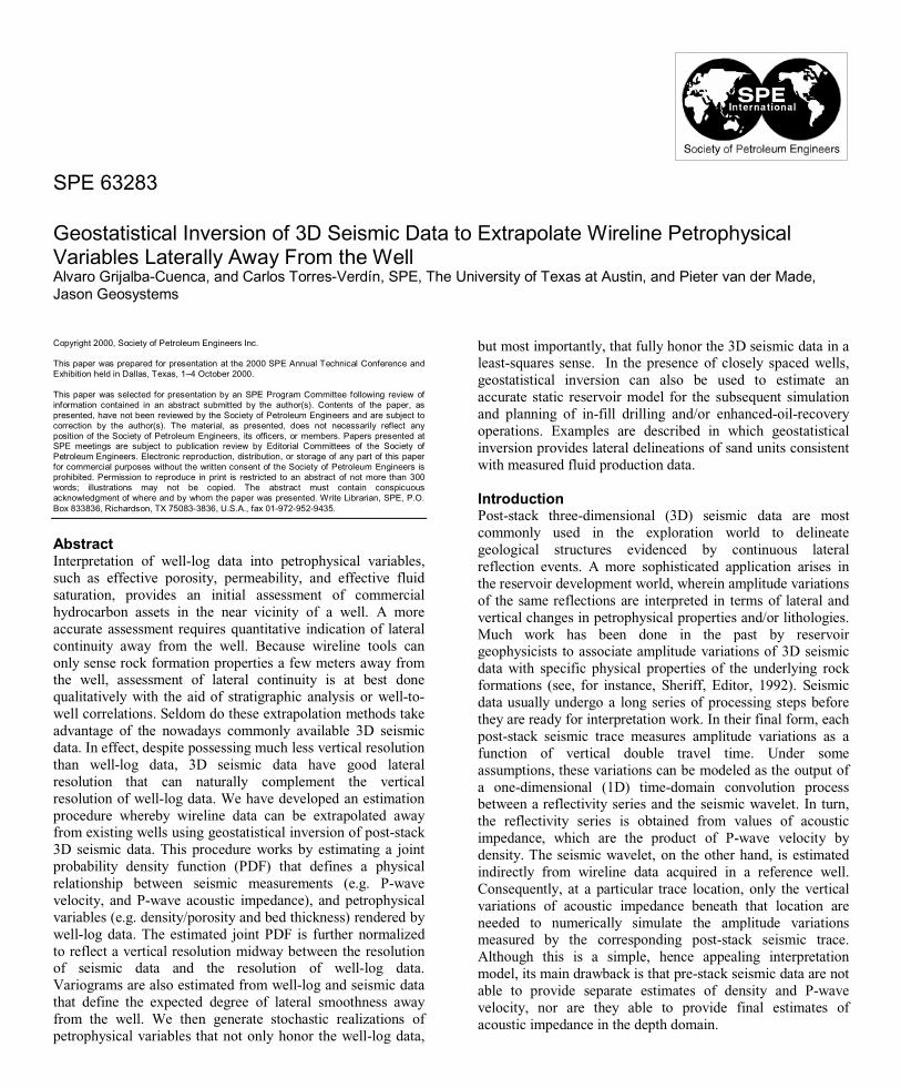
The Data Set and the Local GeologyFigure 1 is a graphical description of the data set used for

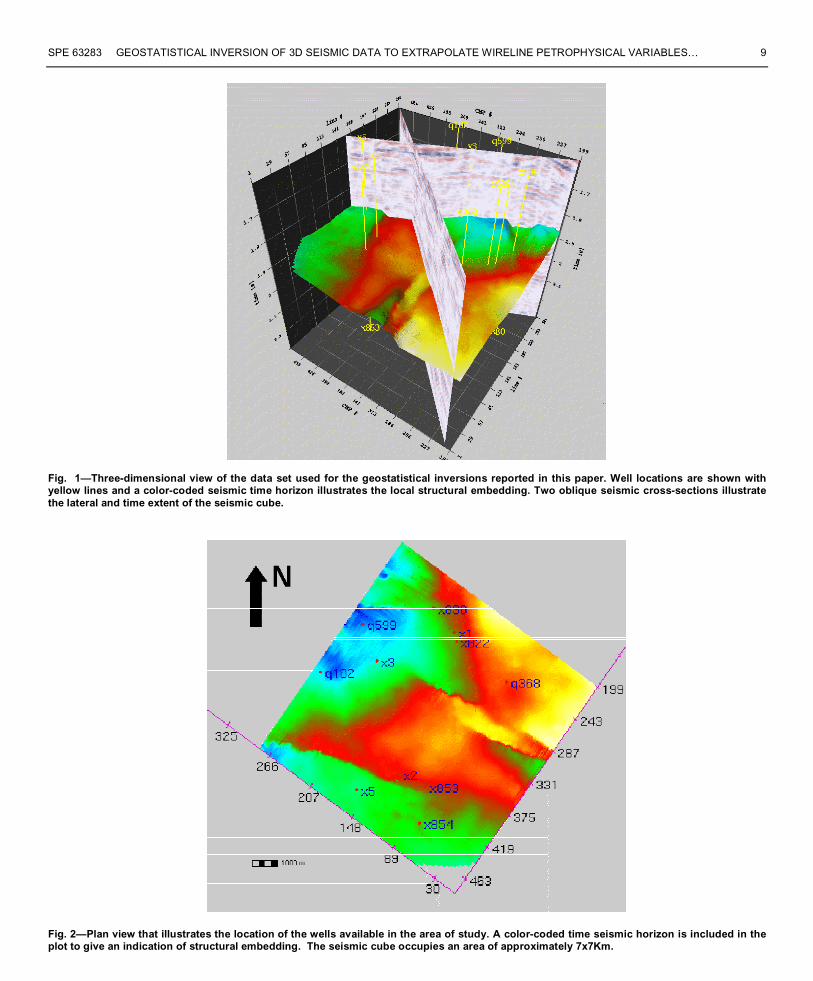
the study reported in this paper. The seismic time horizon andwell locations shown in that figure define an approximately7x7Km subset of a 12x16Km seismic cube acquired in anactive hydrocarbon-producing field. Figure 2 is a plan view of

SPE 63283 GEOSTATISTICAL INVERSION OF 3D SEISMIC DATA TO EXTRAPOLATE WIRELINE PETROPHYSICAL VARIABLES… 3

the study area that shows well locations overlain on top of acolor-coded seismic time horizon. The seismic horizon wasadded to this figure in order to give an indication of theembedding geological structure. A sampling interval of 2msand a bin size of 25m were used to acquire the seismic data.Spectral time analysis evidenced a peak frequency of 35Hz, aphase of approximately 180o, and a maximum usefulfrequency of approximately 85Hz in the seismic responsefrom the subsurface. A cross-section of the post-stack seismicdata that includes three well locations and their associatedacoustic impedance logs is shown in Figure 3. Seismic timehorizons are shown on the same plot for structural andstratigraphic reference.

The hydrocarbon field considered in this study is located inSan Jorge Basin, Argentina. Locally, the sedimentary columncomprises thick shale deposits of lacustrine and flood-plainorigin intercalated with much thinner and laterally sparse andsand bodies. Individual sand units serve as hydrocarbonreservoirs in the depth range from 1,200 to 2,900m below thesurface, and exhibit thicknesses from 0.5 to 15m, but for themost part thinner than 4m.

Given the 10-85Hz spectral content of the seismic data,and assuming an average P-wave velocity value of 3,200m/s(hence a tuning wavelength approximately equal to 12m), itbecomes immediately clear that post-stack seismic data havenot enough vertical resolution to identify individual sand units.Analysis of sonic and density well-log data in the zone ofinterest shows that the velocity of propagation of P-waves ishigher in sands than in shales. On the other hand, the bulkdensity of shales is higher than that of sands. In addition, bothP-wave velocity and density are affected by compaction, morein the case of shales than in the case of sands (the fact thatsands exhibit a higher P-wave velocity than shales is mostlikely due to a difference in mechanical behavior imposed bycompaction). Consequently, in the hydrocarbon-producingdepth interval sands exhibit higher acoustic impedances thanshales. Because post-stack seismic data have no verticalresolution to distinguish individual sands from surroundingshales on the basis of the relative difference in their acousticimpedances, the seismic response can be viewed as theeffective response of sand-shales packets. These sand-shalepackets are defined as rock mixtures with approximately equalproportions of the two lithologies. Our interpretation work hasconsistently showed that sand-shale mixtures thicker than 12mexhibit higher acoustic impedance values than pure shales.This is equivalent to stating that, when shales and sands arestacked together, the acoustic impedance response of the stackremains dominated by that of its sand fraction.

We transformed the existing well-log data into the seismicdouble-travel-time domain using checkshot data. In all casesthe individual well-log transformations were refined with asynthetic seismogram. Whenever it was judged necessary, thelogs were also subjected to an editing process aimed atreducing the deleterious influence of bad borehole calipers inthe density and sonic measurements. A lithology log, termed“lithofrac log” was also estimated for each well to describe anormalized sand proportion value from 0 to 1 (a value of 1

indicates a “pure” sand and a value of 0 indicates a “pure”shale). The lithofrac values were normalized across all of thewells used in this study in an effort to minimize local boreholeeffects in the well-log data, and hence to facilitate well-to-wellpetrophysical evaluations.

Seismic wavelets were estimated for each of the availablewells. An average wavelet was also estimated which wasutilized for global computations. The average wavelet used inthis study is shown in Figure 4 both in the time and frequencydomains Given that the amount of seismic data considered inthis study was many times larger than the available amount ofwell-log data, we chose to work exclusively in the seismicdouble-travel-time domain.

Petrophysical Analysis and Vertical ResolutionFigure 5 is a plot of acoustic impedance vs. bulk densityconstructed from well-log data acquired in one of the studywells. This cross-plot naturally separates three existingcompaction zones in the zone of interest, here termed zones A,B, and C, respectively. The depth boundaries of suchcompartments were easily identified in all the existing wells,and were transformed into the time domain to providereference markers to the seismic data. Subsequently, seismictime horizons were tied to these markers and laterallyfollowed across the complete seismic cube to determine thelocal structural and stratigraphic embedding. The four seismichorizons considered in this study are depicted in Figures 3.

In order to understand the relationship that acousticimpedance bears with lithology, we constructed a cross-plotsimilar to that of Figure 3 for compartment B. This cross-plotis shown in Figure 6. There are three lithology types identifiedin the cross-plot shown in Figure 6, namely, porous sands,tight sands, and shales/tuffs. One can readily see that acousticimpedance alone in this particular case is unable to distinguishthe three types of lithology, i.e. the same value of acousticimpedance could be associated with porous sands, tight sands,or shales/tuffs. Conversely, the same cross-plot indicates thatbulk density could be used to make an accurate distinctionbetween the three types of lithology. Because 3D seismic datacannot separate density and velocity from acoustic impedance,the obvious conclusion from this exercise is that, even if itwere sampled with a vertical resolution similar to that of well-log data, post-stack seismic data alone could not be used toidentify lithology groups. The only possible way to have theseismic data yield separate estimates of density and velocitywould be to subject them to more specialized pre-stackprocessing and inversion techniques. Although this is an ideaworth pursuing, in the present paper we confine ourselves tothe interpretation of post-stack seismic data and leave theexciting topic of pre-stack seismic data interpretation for afuture, more ambitious publication.

We performed an additional exercise to understand therelationship borne by acoustic impedance and lithology as afunction of the vertical resolution of the data. This wasaccomplished by first transforming the well-log data into theseismic double-travel-time domain. The time-domain well-logdata were then resampled with sampling intervals of 0.5, 1,

4 A. GRIJALBA-CUENCA, C. TORRES-VERDIN, P. VAN DER MADE SPE 63283

and 2ms. Subsequently, cross-plots of acoustic impedance andbulk density were constructed within compartment B for thethree resampled groups of data. These cross-plots are shown inFigure 7. We observe that the value range exhibited by bothacoustic impedance and density remain a function of thesampling interval. The cross-plots of Figure 7 also indicatethat an increase in sampling rate causes the porous sands toexhibit higher acoustic impedances that those of the tworemaining lithologies.

The resolution-dependent cross-plots between acousticimpedance and density can be viewed as primitive versions ofjoint probability density functions (PDF’s) between the twovariables. A joint PDF could be assigned to each particularlithology group. For instance, Figure 8, shows how for aparticular lithology group (in this case shales/tuffs) a jointPDF (or cloud transform) between density and acousticimpedance could be first constructed by enforcing density binsor subclasses. Each density bin would be assigned a specificGaussian PDF to define the corresponding range andvariability of acoustic impedances. The complete set ofdensity bins and their corresponding Gaussian PDF’s foracoustic impedance would in turn define a continuous jointPDF between density and acoustic impedance.

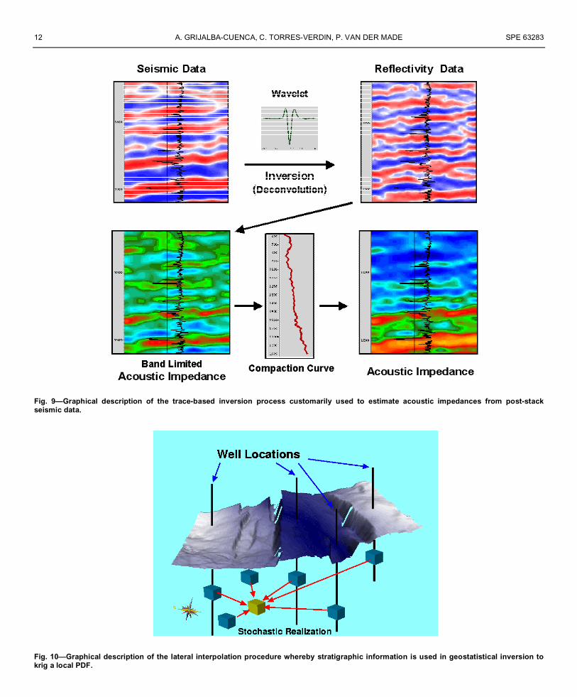
Trace-Based Inversion of the 3D Seismic DataAs emphasized earlier, post-stack seismic data are onlysensitive to acoustic impedances as a function of verticaltravel time. Moreover, because the post-stack seismic data areconstructed to be equivalent to the 1D convolution of aseismic wavelet with the reflectivity series, seismic amplitudevariations remain influenced by the seismic wavelet. Toeffectively respond to subsurface properties, i.e. in order tosolely respond to acoustic impedances, post-stack seismictraces need to be devoid of their wavelet signature. Theprocess whereby post-stack seismic traces are devoid of theirwavelet signature and hence transformed into a reflectivityseries is referred to as deconvolution, or trace-based inversion.Figure 9 is a description of the trace-based inversion processillustrated with data from our project. One can clearly seefrom Figure 9 that the reflectivity data yielded by trace-basedinversion exhibit higher vertical resolution than the originalseismic data.

Acoustic impedances can be obtained from the reflectivitydata by a simple substitution process. This substitution processyields the so-called “raw” or band limited acousticimpedances. The latter are specifically referred to as “bandlimited” because they lack the low-frequency componentsotherwise available in well-log acoustic impedances. Low-frequency components of acoustic impedance define the drifttrend typically seen in wireline logs due to compaction. Theyare missing in the band limited acoustic impedances simplybecause by construction neither the seismic wavelet nor thereflection coefficients are sensitive to them. The only way toinclude the compaction trend in the band limited acousticimpedances is to interpolate it from the compaction trendmeasured along existing wells in the project. Severaltechniques have been put forth to perform the numerical

interpolation of compaction trends, including the use ofstratigraphic and structural control rendered by seismic timehorizons. Reliable results can only be expected with theavailability of closely spaced well and good quality well-logdata. Figure 9 shows the final acoustic impedances derivedfrom trace-based inversion of the post-stack seismic data. Forcomparison, in the same figure we have plotted the location ofa control well and its corresponding lithofrac log. We observethat high values of acoustic impedance correlate well withsand units indicated by local maxima in the lithofrac log.

The particular algorithm used in this paper to deriveacoustic impedances from post-stack seismic data is one dueto Debeye and Van Riel (1990). Rather than solving directlyfor the reflectivity coefficients, Debeye and Van Riel pose thesolution to the inverse problem to yield band limited acousticimpedances and further subject the solution to satisfy time-dependent value-range constraints.

In the end, acoustic impedances yielded by trace-basedinversion can be thought of as the smooth version of thewireline acoustic impedance log that would otherwise beacquired in a vertical well drilled at the particular tracelocation.

Geostatistical Inversion of Acoustic ImpedancesOne of the most attractive properties of geostatisticaltechniques is that they can readily incorporate structural andstratigraphic constraints in their simulations of subsurfacedistributions. By contrast, the same constraints cannot beeasily implemented in trace-based inversion techniques.Seldom can the subsurface be described with standard modelsof Cartesian geometry, and the possibility of using a trulygeological framework has an immediate practical appeal.Structural and stratigraphic information is usually available inthe form of time horizons picked across the seismic cube by anexperienced interpreter. A second important property ofgeostatistical techniques is their flexibility to assimilatedifferent measures of spatial correlation (lateral smoothness)in their simulations of subsurface distributions. Lastly, incontrast with trace-based inversion procedures, geostatisticaltechniques are designed to fully honor the available well-logdata.

Without loss of generality, in this paper we concentrateexclusively on property simulations performed in the seismicdouble-travel-time domain. As an introductory example, let usconsider the stochastic simulation of acoustic impedances.

Figure 10 is a pictorial introduction to our geostatisticalinversion algorithm. In the presence of well-log data andseismic time horizons, the acoustic impedance at a particularpoint in lateral space and vertical time is obtained fromexisting control points. As indicated in Figure 10, the timelocation of these control points is consistent with thegeometrical embedding imposed by the seismic time horizons(and faults). Each control point is described not only with avalue of acoustic impedance but also with a local PDF ofacoustic impedance. At the outset of the algorithm, the PDF ata given control point is estimated from global measurementsof acoustic impedance. One choice is to sample this prior PDF

SPE 63283 GEOSTATISTICAL INVERSION OF 3D SEISMIC DATA TO EXTRAPOLATE WIRELINE PETROPHYSICAL VARIABLES… 5

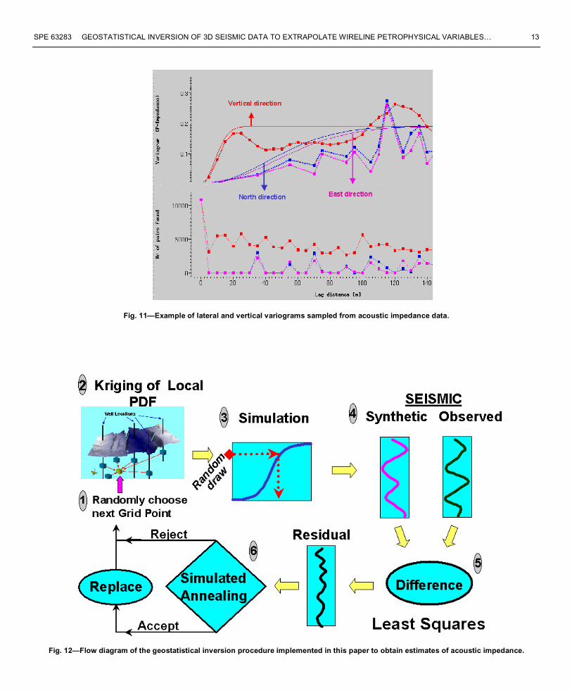
both from both the wireline acoustic impedances the acousticimpedances yielded by trace-based inversion. The firstobjective is to estimate a local PDF at the point where a valueof acoustic impedance is to be simulated. This local PDF isestimated from the PDF’s associated with the available controlpoints by a standard kriging technique (see, for instance,Chilès and Delfiner, 1999 for a superb modern treatment ofgeostatistical concepts and techniques). The kriging operationrequires lateral and vertical variograms, plus knowledge of thedistance that exists between the simulation point and all of thecontrol points. Figure 11 shows examples of vertical andhorizontal variograms of acoustic impedance estimated fromboth well-log acoustic impedances and acoustic impedancesyielded by trace-based inversion. Lateral variograms inparticular, are best estimated from trace-based invertedacoustic impedances because of their relative high lateralsampling rate (in this case 25m).

Once the local PDF has been estimated, the associatedcumulative PDF, or CDF, can be used to make a random drawof acoustic impedance via standard Monte Carlo techniques.In geostatistics, this stochastic simulation procedure has beentraditionally referred to as collocated simulation (Chilès andDelfiner, 1999). The variation of this procedure that isimplemented by geostatistical inversion is the one in whichnot only is the acoustic impedance value randomly drawnfrom the estimated CDF, but also is this value subjected to aperformance test. The performance test consists of (a)computing a local reflectivity series from the simulated valuesof acoustic impedance, (b) convolving the seismic waveletwith the reflectivity series to numerically simulate a localseismic trace, and (c) computing the seismic residual, or sumof square differences, between the simulated seismic trace andthe measured seismic trace.

Upon computing the seismic residual a decision has to bemade to either accept or reject the simulation of acousticimpedance. In our case, we will only accept simulations ofacoustic impedance that entail seismic residuals equal orsmaller than 1%. Whenever the simulated acoustic impedancedoes not pass the acceptance test, a new random draw is madefrom the same CDF. The critical step in this procedure is tomake the next random draw such that the correspondingresidual will be closer to passing the 1% acceptance test tan inthe previous draw, otherwise the search may require a greatmany trials before making a successful draw. There existmany ways to make a new, more “educated” random drawfrom the CDF that will guarantee a smaller seismic residual(see, for instance, Sen and Stoffa, 1995, and Mosegaard andTarantola, 1995). In this paper we have implemented asimulated annealing algorithm to smoothly “step” through theCDF. This algorithm is designed to allow up to a prescribedmaximum number of trials (or iterations) before reaching thedesired 1% seismic residual. Whenever the simulations havenot reached the desired value of seismic residual within theallotted number of trials, the simulated annealing procedureterminates and the current acoustic impedance realization ischosen as the final result. Simulated annealing algorithms alsonaturally lend themselves to computer implementations in

parallel processors, in which case the search for a successfulrandom draw can be accelerated in proportion to the numberof available computer processors. The option to use dualcomputer processors has also been implemented in oursimulated annealing algorithm, and this has reduced by 50%the total CPU time required to perform the simulationsreported in this paper.

Figure 12 is a flow diagram of the geostatistical inversionalgorithm described above. Once a satisfactory localsimulation of acoustic impedance is performed, the search isdirected to a new point in the seismic cube, and the randomselection process described in Figure 12 repeats itself. Newsimulation points (both laterally as well as in time) are alsorandomly chosen until the complete distribution of acousticimpedance populates the seismic cube.

Because the seismic wavelet is not a single-time domainfunction but rather extends along a finite time interval(typically 100ms), a single-time acoustic impedancesimulation is not sufficient to compute the seismic residuals.To solve this technical problem, a stochastic simulations ofacoustic impedance is not only obtained at any given point inthe cube, but also at adjacent time locations above and belowthis point until a time interval is covered equal in length to thatof the seismic wavelet.

Another important technical detail of the geostatisticalinversion algorithm concerns the interpolation (kriging) of thelocal PDF. As emphasized earlier in conjunction with trace-based inversion, the inversion of post-stack seismic data intoacoustic impedances cannot recover the low-frequencycomponents of the latter. In other words, one can fully honorthe seismic data even if the low-frequency components of theacoustic impedances are absent. To solve this problem in ouralgorithm, interpolation of the local PDF is performed viaordinary kriging, as opposed to simple krigging techniques(Chilès and Delfiner, 1999). Ordinary kriging techniquesmaintain the average value of the acoustic impedancemeasured at control points. This operation in some waysimplicitly enforces the numerical interpolation of compactiontrends otherwise done separately in trace-based inversionalgorithms.

In general, the solution to the inverse problem is non-unique, i.e. there are many possible distributions of acousticimpedance that can fully honor both the well-log and seismicdata. Similar to stochastic geostatistical simulation algorithms,geostatistical inversion provides a simple, almost trivial wayto quantify non-uniqueness (uncertainty) in the estimates. Thisis done by literally running the same simulation/inversionalgorithm as many times as needed. Within the limits imposedby finite-precision computer arithmetic, each geostatisticalinversion provides an independent estimate of acousticimpedance, whereupon the complete set of simulations canused to quantify local uncertainty. In this paper we have useda relatively fast way to provide as many independentsimulations as needed of acoustic impedance. This methodconsists of locally repeating the random search process fromthe same PDF as many times as simulations have beenrequested. In other words, rather than performing one

6 A. GRIJALBA-CUENCA, C. TORRES-VERDIN, P. VAN DER MADE SPE 63283

complete simulation over the entire seismic cube, and thenstarting the process over again as many times as simulationshave been requested, we remain at the same point while thegeostatistical inversion is repeated with as many seeds asneeded to produce the number of requested independentsimulations of acoustic impedance. Therefore, after all of thepoints in the seismic cube have been visited by thegeostatistical inversion algorithm, results become available foras many independent simulations as initially requested.Whenever parallel computer processors are available to solvethis simulation problem, different independent simulations canbe simultaneously performed in different processors.

Figure 13 is a composite plot that illustrates cross-sectionsof acoustic impedance obtained with the geostatisticalinversion described above. There are four panels in that figure.The upper left-hand panel describes the input seismic andwell-log data, whereas the upper right-hand panel describesthe corresponding acoustic impedances obtained via trace-based inversion. Acoustic impedances obtained withgeostatistical inversion are shown in the lower left-hand panel.Lastly, and for comparison, standard geostatistical simulationsof acoustic impedance are shown in the lower right-handpanel. All of the simulations shown in Figure 13 wereperformed with a time sampling rate of 2ms. Results shownfor both geostatistical simulation and geostatistical inversionrepresent the average of 10 independent simulations. Wirelineacoustic impedance data from the three wells shown in Figure13 were used to produce the simulations. These acousticimpedance logs were previously down-sampled (low-passfiltered and resampled) to the 2ms sampling rate exhibited bythe seismic data. The same set of variograms and prior PDF’swere used to obtain both the standard geostatisticalsimulations and the geostatistical inversions. Quite clearly, thegeostatistical inversion results correlate very well with thetrace-based inversion results, whereas the standardgeostatistical simulations correlate poorly with them. Figure14 shows cross-sections of standard deviation associated withthe two sets of 10 independent simulations of acousticimpedance. The left-hand panel in that figure shows thestandard deviation for the conventional geostatisticalsimulations, whereas the right-hand panel shows the standarddeviation for the geostatistical inversions. As evidenced bythese cross-sections, in our work we have consistently foundthat the standard deviations associated with geostatisticalinversion are much smaller than those of standardgeostatistical simulations.

We have also performed sensitivity analysis to quantify theinfluence that a small change in the lateral and verticalvariograms, i.e. a change in their sills and ranges, can have onthe corresponding simulations of acoustic impedance. Thisexercise showed that changes of 25% or less in both sill andrange did not visibly modify the corresponding geostatisticalinversion results. By contrast, we found that the standardgeostatistical simulations were significantly affected by thesame changes in the variograms. A similar sensitivity analysiswas performed to determine the influence of the prior PDF onthe corresponding geostatistical inversions of acoustic

impedance. This analysis showed that the prior PDF couldhave a significant effect in reducing or increasing the CPUtimes required to perform the simulations. A narrow PDFwould tend to accelerate the solution, but would also tend toproduce higher than acceptable seismic residuals. Conversely,a wide PDF would entail lower seismic residuals but wouldoften prompt excessively large CPU times to perform thesimulations.

Geostatistical Inversion of Density and LithologyThe power and flexibility of geostatistical inversion is bestunderstood when performing estimations of petrophysicalvariables directly or indirectly correlated with acousticimpedance. Correlations of such nature may ultimately bedescribed with a joint PDF, for instance, of the type illustratedin Figure 8 between density and acoustic impedance. From theviewpoint of geostatistical inversion, it is desirable to enforcea correlation between petrophysical variables and acousticimpedance. Such a correlation could then be used to constrainthe petrophysical simulations between existing wells to honorthe post-stack 3D seismic data.

As an example, consider again the cross-plot shown inFigure 6. In this cross-plot the relationship between acousticimpedance and density (and indirectly with porosity) is notonly in the form of a joint PDF, but it is also lithologydependent. Thus, if one were to simulate density (or porosity)to in turn simulate acoustic impedance, prior knowledge of thespecific lithology group would be necessary. A way to solvethis problem would be to simulate the lithology type in thefirst place using a lithology PDF (in this case consisting ofonly three possibilities, porous sands, tight sands, andshales/tuffs). After a lithology type is simulated from thelithology PDF, one could draw a random sample of densityfrom a density PDF previously estimated for that particularlithology group. The simulated value of density would befinally used to draw a random sample of acoustic impedancevia the joint PDF that relates density with acoustic impedance.Such is precisely the procedure we have implemented in thispaper to estimate lithology and bulk density in the inter-wellregion while enforcing an adequate match with the post-stack3D seismic data.

We estimated the lithology PDF’s from lithology logssynthesized from the available wireline data. Density PDF’sfor each lithology group were also estimated from theavailable wireline data. Variogram analysis considered all ofthe available wireline data plus the acoustic impedancesobtained from trace-based inversion. The vertical variogramsfor lithology and for lithology-dependent density wereestimated from the wireline data., and the lateral variogramsfor both lithology and density were adapted from the lateralvariograms of acoustic impedance. Lastly, in order for thesimulations to resolve individual sand units, the geostatisticalinversions were performed with a vertical resolution betterthan 2ms. We considered simulations with 0.5 and 1msresolution, and all of the PDF’s and variograms supporting thesimulations were made consistent with these time samplingintervals.

SPE 63283 GEOSTATISTICAL INVERSION OF 3D SEISMIC DATA TO EXTRAPOLATE WIRELINE PETROPHYSICAL VARIABLES… 7

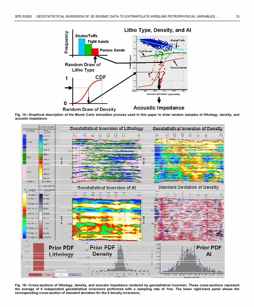
Figure 15 is a schematic description of the process wehave used to draw final random samples of acousticimpedance from random draws of lithology and density. Fist,in analogy with the process described earlier to simulateacoustic impedances, at a given point in the seismic cube alocal lithology PDF was kriged from PDF’s measured atexisting control points. An ordinary kriging procedure wasused to obtain this local PDF. From the corresponding CDF, aMonte Carlo simulation was run to yield a random realizationof lithology (a porous sand in the example shown in Figure15). Once the lithology group became defined, a density PDFwas kriged that was consistent with that lithology group. Thevariograms used for this ordinary kriging operation were alsoconsistent with the previously simulated lithology group.Subsequently, the kriged density PDF was used to calculate aCDF and from this a random draw was made. The value ofdensity that resulted from this process was input to the jointPDF between density and acoustic impedance to in turnprovide a random draw of acoustic impedance. Finally, thesimulated value of acoustic impedance was subjected to thesame quality control test described in Figure 12 to determinewhether the post-stack seismic data were honored within a 1%relative error. Failure to do so immediately prompted asimulated annealing algorithm to command an efficient searchof new lithology and density values until a 1% seismicresidual was secured within the allotted number of trials. Thesame process was repeated at every point within the seismiccube and for as many independent simulations as requestedbeforehand. At the end of the geostatistical inversion process,high-resolution cubes of lithology and density were providedwhich fully honored the available 3D seismic data.

Of course, there is a strong assumption of stationarityimplicit in the above simulation procedure. Not only are wemaking the assumption that the variograms are stationary, butalso that the joint PDF between acoustic impedance anddensity remains independent of space. By estimating differentsets of variograms, and of acoustic impedance-density PDF’sin the 3 reservoir zones described in Figure 3, we have madean attempt to reduce the sensitivity of our results to an error inthe assumption of stationarity. Although we feel that oursimulations are sufficiently local to support this assumption, itis obvious that more work is needed to quantify itsimplications.

Figure 16 is a composite plot that shows cross-sections oflithology and density rendered by the geostatistical inversionprocedure described above. These cross-sections represent anaverage of a total of 6 independent inversions obtained with avertical resolution of 1ms. For completeness and reference,Figure 16 also shows a cross-section of acoustic impedancesobtained with geostatistical inversion, and a cross-section ofstandard deviation values obtained from the 6 independentdensity inversions. We observe an excellent consistencybetween the lithology, density, and acoustic impedancesimulations. Moreover, the variability of the density estimatesin the inter-well region is quite acceptable. The complete setof 6 geostatistical inversions whose means are shown inFigure 16 were computed with a dual-CPU Octane, SGI

workstation and this required approximately 36 hours of CPUtime.

In Figure 17 we show plan views of the correlationbetween the measured and simulated seismic data setsassociated with the inversions of Figure 1. There is one planview of seismic correlation for each of the 6 independentgeostatistical inversions of density. The correlations areacceptably high and lend excellent credence to thegeostatistical simulations. A final illustration of the lithologyinversion is presented in Figure 18. In this 3D image we haveonly included samples in the seismic cube corresponding toporous sands, and have explored the connectivity of thesesands with a special graphical utility. A total of 13 sand unitsare shown in 3D view in Figure 18. Some of these sand unitsdo extend from one well to another, but other sands remainisolated or else only intersected by one of the wells. Needlessto say, the 3D connectivity maps of Figure 18 are an excellentway to assess the lateral continuity of petrophysical featuresaway from existing wells. They are a powerful final productfrom the geostatistical inversions that can be further utilized todefine static and/or dynamic reservoir models. Oncetransformed into depth, these models can be directly input toreservoir simulators to perform production forecasts, and toassess the impact of in-fill and/or enhanced-oil-recoveryoperations. In our study we have found the 3D lithology mapsof Figure 18 to be consistent with total fluid productionvolumes withdrawn from individual sand units.

ConclusionsExtrapolation of wireline petrophysical variables laterallyaway from wells can be performed by combining theinformation content of well-log and post-stack 3D seismicdata. We have successfully shown that geostatistical inversionprovides a flexible, quantitative framework to accomplish thisobjective. Our procedure hinges upon the assumption thatacoustic impedance bears a correlation with the petrophysicalvariable under study. This correlation can be expressed in theform a joint PDF constructed from cross-plots and histogramsof available data. The joint PDF is also to be consistent withthe vertical sampling interval chosen to perform theextrapolation. Usually this sampling interval is somewherebetween the vertical resolution of the well-log and seismicdata sets. Access to a joint PDF between acoustic impedanceand the petrophysical variable under study provides a directway to enforce a solution to the extrapolation problem thatfully honors the post-stack 3D seismic data.

Geostatistical inversion constructs an extrapolation of thepetrophysical variable via stochastic simulation techniques.This means that the value assigned to the petrophysicalvariable at a point away from existing wells is obtained fromthe random draw from a PDF. The latter PDF is constructedusing lateral correlation concepts and techniques derived fromthe field of geostatistics. In this paper, we have implemented astochastic simulation procedure based on simulated annealingto further condition the simulations to honor the seismic datawithin a 1% relative least-squares error. The simulatedannealing procedure used in this paper has allowed us to

8 A. GRIJALBA-CUENCA, C. TORRES-VERDIN, P. VAN DER MADE SPE 63283

obtain multiple realizations of petrophysical variables withinreasonable CPU times and for relatively large seismic cubes.Computation times can be further reduced with the use ofmultiple-processor computers, and this is also a solutionamenable to simulated annealing.

The example problem considered in this paper provided adifficult test for the geostatistical inversion formulation. Notonly were sand units thinner than seismic tuning resolution,but also the relationship borne by acoustic impedance anddensity was non-unique. We successfully showed that thestochastic formulation behind geostatistical inversion wasflexible enough to warrant a solution to our test problem. Thissolution was consistent with fluid production data and withwell-to-well correlations.

In the future, we will study the possibility of implementinga geostatistical formulation to invert pre-stack 3D seismic datainto reservoir parameters away from wells. We will alsocontinue to explore ways to expedite the inversion algorithm.

AcknowledgementsWe would like to express our gratitude to Repsol-YPF forpermission to use their 3D seismic and well-log data set fromCañadón de la Escondida, Chubut, Argentina.

References1. Chilès, J.-P., and Delfiner, P.: Geostatistics, John Wiley and

Sons, Inc., New York (1999).2. Debeye, H. W. J., and Van Riel, P.: “Lp-Norm Deconvolution,”

Geophysical Prospecting (1990) 38, 381-403.3. Haas, A., and Dubrule, O.: “Geostatistical Inversion –A

Sequential Method for Stochastic Reservoir ModellingConstrained by Seismic Data,” First Break (1994) 12, no. 11,561-569.

4. Journel, A. G., and Huijbregts, C. J.: “Geostatistical ReservoirCharacterization Constrained by 3D Seismic Data,” 1978 58th

Annual International Meeting of the European Association ofExploration Geophysicists.

5. Mosegaard, K., and Tarantola, A.: “Monte Carlo Sampling ofSolutions to Inverse Problems,” J. Geophys. Res. (1995) 100, no.12, 431-447.

6. Pendrel, J. V., and Van Riel, P.: “Estimating Porosity From 3DSeismic Inversion and 3D Geostatistics,” 1997 67th AnnualInternational Meeting of the Society of ExplorationGeophysicists.

7. Sen, M. K., and Stoffa, P. L.: Global Optimization Methods inGeophysical Inversion, Volume 4 of Advances in ExplorationGeophysics, Elseviere, Amsterdam (1995).

8. Sheriff, R. E., Editor: Reservoir Geophysics, Investigations inGeophysics Series, Volume 7, Society of ExplorationGeophysicists, Tulsa (1992).

9. Torres-Verdín, C., Victoria, M., Merletti, G., and Pendrel, J. V.:“Trace-Based and Geostatistical Inversion of 3-D Seismic Datafor Thin-Sand Delineation: An Application to San Jorge Basin,Argentina,” The Leading Edge (September 1999), 1070-1076.

SPE 63283 GEOSTATISTICAL INVERSION OF 3D SEISMIC DATA TO EXTRAPOLATE WIRELINE PETROPHYSICAL VARIABLES… 9

Fig. 1—Three-dimensional view of the data set used for the geostatistical inversions reported in this paper. Well locations are shown withyellow lines and a color-coded seismic time horizon illustrates the local structural embedding. Two oblique seismic cross-sections illustratethe lateral and time extent of the seismic cube.

Fig. 2—Plan view that illustrates the location of the wells available in the area of study. A color-coded time seismic horizon is included in theplot to give an indication of structural embedding. The seismic cube occupies an area of approximately 7x7Km.

10 A. GRIJALBA-CUENCA, C. TORRES-VERDIN, P. VAN DER MADE SPE 63283

Fig. 3—Cross-section of the post-stack 3D seismic data indicating three vertical reservoir compartments. Acoustic impedance logs aredisplayed at the three well locations identified in the cross-section.

Fig. 4—Average wavelet estimated for the seismic data shown in Figures 1 and 3.

Fig. 5—Cross-plot of well-log acoustic impedance and density data. Clusters of points clearly separate the vertical reservoir zones describedin Figure 3.

SPE 63283 GEOSTATISTICAL INVERSION OF 3D SEISMIC DATA TO EXTRAPOLATE WIRELINE PETROPHYSICAL VARIABLES… 11

Fig. 6—Cross-plot of well-log acoustic impedance and density data in Zone B. Different clusters of points are associated with a specificlithology

Fig. 7—Cross-plots of well-log acoustic impedance and density data in Zone B. The cross-plots were constructed in the time domain withthree different sampling rates, i.e. 0.5, 1, and 2 ms.

Fig. 8—Graphical description of the strategy used in this paper to construct a joint PDF between acoustic impedance and density.

12 A. GRIJALBA-CUENCA, C. TORRES-VERDIN, P. VAN DER MADE SPE 63283

Fig. 9—Graphical description of the trace-based inversion process customarily used to estimate acoustic impedances from post-stackseismic data.

Fig. 10—Graphical description of the lateral interpolation procedure whereby stratigraphic information is used in geostatistical inversion tokrig a local PDF.

SPE 63283 GEOSTATISTICAL INVERSION OF 3D SEISMIC DATA TO EXTRAPOLATE WIRELINE PETROPHYSICAL VARIABLES… 13

Fig. 11—Example of lateral and vertical variograms sampled from acoustic impedance data.

Fig. 12—Flow diagram of the geostatistical inversion procedure implemented in this paper to obtain estimates of acoustic impedance.

14 A. GRIJALBA-CUENCA, C. TORRES-VERDIN, P. VAN DER MADE SPE 63283

Fig. 13—Comparison of acoustic impedance cross-sections rendered by (a) trace-based inversion, (b) geostatistical inversion, and (c)conventional geostatistical simulation. All results were produced with a time sampling rate of 2ms. Cross-sections of geostatistical inversionand conventional geostatistical simulation represent the average of 10 independent simulations.

Fig. 14—Cross-sections of standard deviation calculated from 10 independent estimates of acoustic impedance. The left- and right-handpanels are standard deviations associated with conventional geostatistical simulation, and geostatistical inversion, respectively. Theseresults are derived from the simulations illustrated in Figure 13.

SPE 63283 GEOSTATISTICAL INVERSION OF 3D SEISMIC DATA TO EXTRAPOLATE WIRELINE PETROPHYSICAL VARIABLES… 15

Fig. 15—Graphical description of the Monte Carlo simulation process used in this paper to draw random samples of lithology, density, andacoustic impedance.

Fig. 16—Cross-sections of lithology, density, and acoustic impedance rendered by geostatistical inversion. These cross-sections representthe average of 6 independent geostatistical inversions performed with a sampling rate of 1ms. The lower right-hand panel shows thecorresponding cross-section of standard deviation for the 6 density inversions.

16 A. GRIJALBA-CUENCA, C. TORRES-VERDIN, P. VAN DER MADE SPE 63283

Fig. 17—Plan view of the correlation between the measured seismic data and the seismic data simulated while producing the 6 geostatisticalinversions of density described in Figure 16. A seismic correlation map is shown for each of the 6 geostatistical inversions.

Fig. 18—Three-dimensional map of sand connectivity obtained from the geostatistical inversion of lithology described in Figure 16.