Embed Size (px)
Citation preview

1
Topic 11 – ANOVA II
Balanced Two-Way ANOVA
(Chapter 19)

2
Two Way ANOVA
We are now interested the combined effects of two factors, A and B, on a response (note: text refers to these as R = rows and C = columns – we’ll call them A, B, and later C for a 3-way ANOVA). Examples: Want to consider the effects of diet plan (Factor A)
and exercise program (Factor B) on weight.
Want to consider the effects of a drug (Factor A) and a vitamin tablet (Factor B) on blood pressure.

3
Two Way ANOVA (2)
Interested in a combination of the two factors; unlike blocking, both of primary interest.
Could treat each combination of factors as a treatment and do one-way ANOVA, but then you have to use contrasts a lot in order to tests hypotheses of interest.

4
Two Way ANOVA (3)
Interaction is a possibility.
Replication is required to investigate interaction. You generally want at least two observations per treatment combination.
You also generally want a balanced design (for this topic, we’ll assume cell sizes are equal).

5
Example (Problem 19.1)
An animal experiment is designed to investigate whether the drug Levorphanol reduces stress as reflected in the cortical sterone level.
It is also likely that Epinephrine (adrenaline) levels have some effect and there may be an interaction with the drug effect as well. Some animals were given a drug that raised their normal levels of Epinephrine.

6
Example (2)
Control Levorphanol Epinephrine Both
1.90
1.80
1.54
4.10
1.89
0.82
3.36
1.64
1.74
1.21
5.33
4.84
5.26
4.92
6.07
3.08
1.42
4.54
1.25
2.57

7
Example (3)
If we treat this as one-way ANOVA (which is not ideal in real life but useful here for instructional purposes), then we can design contrasts can be used to investigate the effects:
Comparison C L E B
L effect
E effect
Interaction
-1
-1
1
1
-1
-1
-1
1
-1
1
1
1

8
SAS Code (one-way)
proc glm; class trt; model y=trt; contrast 'L' trt -1 1 -1 1; contrast 'E' trt -1 -1 1 1; contrast 'Interaction' trt 1 -1 -1 1; means trt /tukey; run; quit;

9
SAS Output
Source DF SS MS F Value Pr > F Model 3 37.58 12.53 12.30 0.0002 Error 16 16.30 1.02 Total 19 53.88 Contrast DF SS MS F Value Pr > F L 1 12.83 12.83 12.60 0.0027 E 1 18.59 18.59 18.25 0.0006 Interaction 1 6.16 6.16 6.05 0.0257

10
Notes
The three contrasts have a special property – they are “orthogonal”. Their sum is actually the model SS: 12.83 + 18.59 + 6.16 = 37.58.
We see that there are distinguishable effects for both drugs, plus an interaction (F-tests).
A significant interaction means that the size of the L effect is different at different levels of E (or equivalently, the size of the E effect is different for different levels of L); more later.

11
Two-Way ANOVA Break up the treatments into two factors.
Factor 1: Levorphanol (Present / Absent)
Factor 2: Epinephrine (High / Low)
Investigates all combinations of the two factors
Ep.
Lev. Low High
Absent xxxxx xxxxx
Present xxxxx xxxxx

12
Two-Way ANOVA (2)
Rows / Columns of table represent levels of the factors. We have 5 observations at each combination of levels. Another way to view the design:

13
Output from interaction model
Source DF SS MS F Value Pr > F Model 3 37.58 12.53 12.30 0.0002 Error 16 16.30 1.02 Total 19 53.88 Source DF Type I SS MS F Value Pr > F E 1 18.59 18.59 18.25 0.0006 L 1 12.83 12.83 12.60 0.0027 E*L 1 6.16 6.16 6.05 0.0257
Note: Type III SS will be the same, since balanced design.

14
Statistical Model
a levels of Factor A; b levels of Factor B
n observations per cell, so the total number of observations is nab.
Usual basic assumptions: Independent & Normal Errors with Constant Variance.

15
Statistical Model (2)
th
th
1, 2, ...,
1, 2, ...,
1, 2, ...,
2
interaction effect in cell
~ 0, , inde
grand mean level effect of Factor A
level effect of Factor B
i a
j bij i j ijkijk n
i
j
ij
ijk
j
ij
N
i
Y
pendent

16
Statistical Model (3)
As before we think of all the effects in terms of deviation from the grand (overall) mean. We need parameter restrictions:
SAS does things slightly differently – making mu the mean for the last treatment combination (labeled ab), and setting any parameter with one of those levels to zero.
0 0 0 0i j ij iji j

17
Statistical Model (4)
Original ANOVA table (SAS) will have an “overall” F-test.
Simply tests whether ANY of the factors are significant.
Not particularly useful (unless insignificant) as it doesn’t differentiate between the factors.
Because of this, we usually create an “extended” ANOVA table by replacing the model line with the Type I SS.

18
Analysis of Variance Table
Source DF SS MS F0
Factor A SSA MSA MSA/MSE
Factor B SSB MSB MSB/MSE
AB Interaction
SSAB MSAB MSAB/MSE
Error SSE MSE
Total SST
1a 1b
1 1a b
1abn 1ab n

19
Replication
Recall that RCBD typically has n = 1.
Notice what happens in the ANOVA table if we have n = 1.
In this case, we will not be able to investigate interaction as the DF for error would be zero (interaction and error effects would be confounded, or inseparable – a different type of “confounding” than we discussed last time).
We need at least two replicates in order to assess interaction.

20
Breakdown of SS
As before, don’t worry too much about the formulas in the book. Do remember:
SSModel + SSError = SSTotal
SSModel gets broken down via the Type I SS
For balanced design, Type III SS will all be the same as Type I SS. Balanced designs are to be preferred.
Know other relationships within the ANOVA table and how to put together test statistics.

21
Tests
There is a specific order in which you need to do the tests.
General Rule of Thumb: Test higher order terms first.
If higher order terms are significant (say AB interaction), then tests for lower order terms (A and B main effects) do not matter as much.
Why?

22
Test for Interaction
F-statistic:
Hypotheses
If
then reject H0.
If insignificant, then can test for main effects.
/F MSAB MSE
0 : 0 for all ,
: There is some non-zero
ij
a ij
H i j
H
0.05, 1 1 , 1num denDF a b DF ab nF F

23
Test for Main Effect Factor A
F-statistic:
Hypotheses
If then reject H0
/F MSA MSE
0 1 2: ... 0
: There is some non-zero a
a i
H
H
0.05, 1, 1num denDF a DF ab nF F

24
Test for Main Effect Factor B
F-statistic:
Hypotheses
If then reject H0.
/F MSB MSE
0 1 2: ... 0
: There is some non-zero b
a j
H
H
0.05, 1, 1num denDF b DF ab nF F

25
Comparing Factors / Levels
If there is an interaction – you must do comparisons for one factor at each level of the other factor. (More later)
If a main effect tests significant (whether or not there is interaction), you can study the main effect by averaging over all levels of the other factor.
This will be most meaningful if there truly is no interaction; when interaction is present, still best to study it first.
26
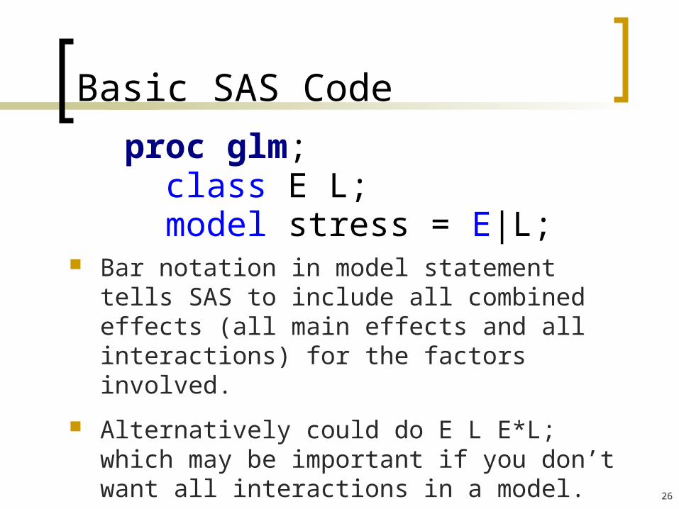
Basic SAS Code
Bar notation in model statement tells SAS to include all combined effects (all main effects and all interactions) for the factors involved.
Alternatively could do E L E*L; which may be important if you don’t want all interactions in a model.
proc glm; class E L; model stress = E|L;

27
Output from interaction model
Source DF SS MS F Value Pr > F Model 3 37.58 12.53 12.30 0.0002 Error 16 16.30 1.02 Total 19 53.88 Source DF Type I SS MS F Value Pr > F E 1 18.59 18.59 18.25 0.0006 L 1 12.83 12.83 12.60 0.0027 E*L 1 6.16 6.16 6.05 0.0257
Note: Type III SS will be the same, since balanced design.

28
Create “Extended” Table
Source DF SS MS F Value Pr > F E 1 18.59 18.59 18.25 0.0006 L 1 12.83 12.83 12.60 0.0027 E*L 1 6.16 6.16 6.05 0.0257 Error 16 16.30 1.02 Total 19 53.88
The Type I SS lines replace the model line. This makes it easy to see not only that there are significant effects, but which effects in particular are important.

29
Where next?
Interaction is significant, so we will want to study that.
Because main effects are also significant, we will be able to distinguish them to some extent from the interaction.
Our statements about the main effects, however, will be less useful than they would be if there were no interaction.

30
Computing main the effects
The means for each combination are
Compare Levorphanol (average out epin.)
Low E High E
L Absent 2.246 5.284
L Present 1.754 2.572
1.754 2.572 2.246 5.2841.602
2 2

31
Main Effects (2)
Adding L results in a significant decrease in stress levels for the animals.
Compare Epinephrine (average out lev.)
Higher levels of E result in significant increases in the stress levels.
5.284 2.572 2.246 1.7541.928
2 2

32
Interaction
What about the interaction?
Difference in effect of L between low E and high E:
This says that the effect size for the use of L is much larger when E levels are high. You get a greater reduction in stress (or more bang for your buck).
2.572 5.284 1.754 2.2462.712 0.492 2.220

33
Interaction (2)
You could go the other way and consider:
Difference in effect of E when L is used (vs. not used):
Interpretation: The effect size for having higher levels of E is smaller when the drug L is used.
2.572 1.754 5.284 2.2460.818 3.038 2.220

34
Conclusions
Higher levels of E result in greater stress (as we might expect).
The drug L seems to effectively lower stress levels regardless of E levels. But it works more efficiently at higher levels of E and lowers stress levels by a greater amount.

35
Interactions
When there is significant interaction, the key to the analysis is studying the interaction and interpreting it.

36
Interaction Plots
Two choices:
Plot MEAN Response vs. Factor B by Factor A
Plot MEAN Response vs. Factor A by Factor B
Possible outcomes include Main Effects but No Interaction One Main Effect but No Interaction Same Direction Interaction (as in example; increase
or decrease, but not by same amount) Reverse Interaction See Section 19-6-2.

37
Interaction Plots
We’ll now take a look at a number of 2 x 2 interaction plots to get an idea of what to look for.
Once you learn to look at the plots, you will be able to:
Determine if interaction is present
Estimate effect sizes from the plots

38
Interaction Plots (1)
Main Effects, No Interaction
39
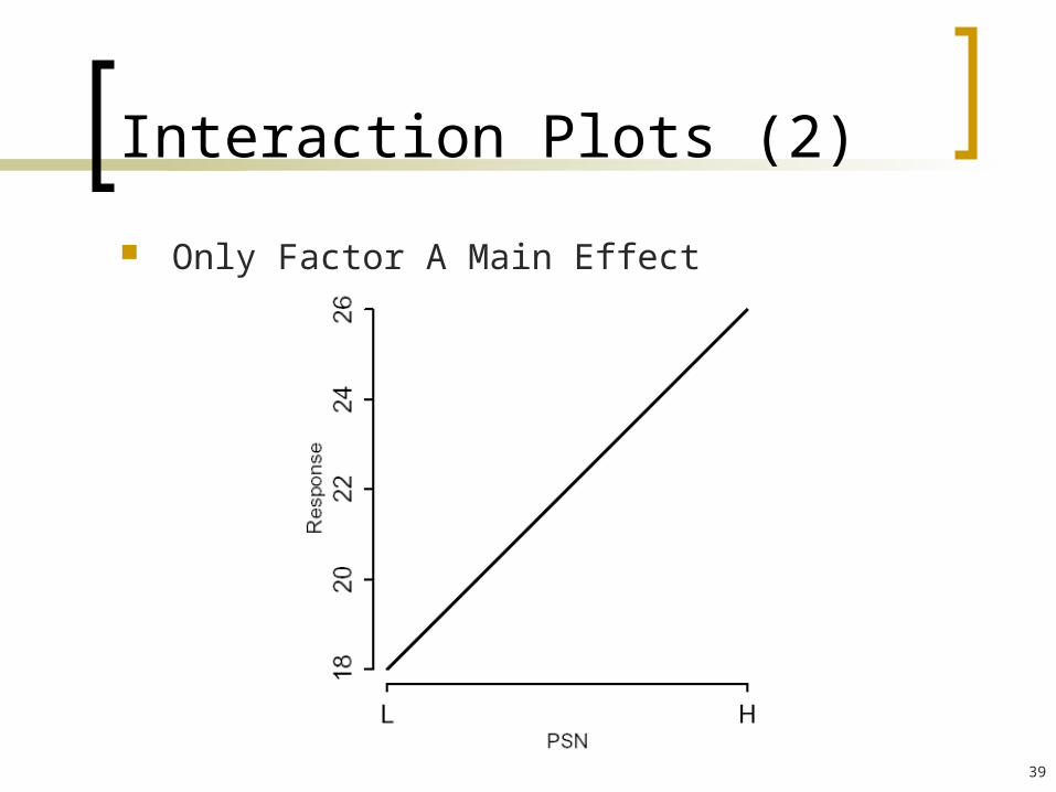
Interaction Plots (2)
Only Factor A Main Effect

40
Interaction Plots (3)
Decreasing A effect, but not by same amt.

41
Interaction Plots (4)
Reverse Interaction (Main effects likely appear insignificant due to the interaction)

42
Key to Interpretation
If interaction is present, then the effect of one factor depends on the level of the other factor. Hence main effects carry explicit meaning only if
we have no interaction.
If opposite behavior (as on the previous slide), main effect might be cancelled out by the interaction and appear insignificant.
When interaction is present, you need to discuss the effect of each variable at a specific level of the other (cannot separate).

43
Example
We return to our example
Difference in effect of L based on E = high or low:
Can we test for significance?
Need to develop standard errors.
2.712 0.492
High E Low E

44
Example (2)
From ANOVA table, MSE = 1.019 on 16 degrees of freedom. For any two-sided t-test, the critical value for significance level 0.05 will be 2.12.
For E = low, the estimated L effect is -0.492 (see previous slide). The standard error for that difference would be
So T = -0.492/0.6384 = -0.77. We conclude that the L effect is not significantly different from 0 for low E.
For E = high, estimated effect of L is -2.712 with SE of 0.6384. Hence T = -4.25. and we conclude that the L effect is a significant decrease for high E.
1.019 1/ 5 1/ 5 0.6384

45
Obtaining these tests from SAS
First note that the minor calculations we’ve done in the notes you should be able to put together by hand.
In SAS, we’ll use the LSMEANS statement in PROC GLM, and can get all the numbers we have computed.
New: As an option in LSMeans for the interaction A*B, use SLICE = <B> to obtain tests for the significance of Factor A at fixed levels of Factor B.
46
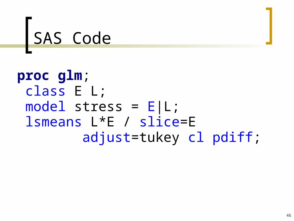
SAS Code
proc glm; class E L; model stress = E|L; lsmeans L*E / slice=E adjust=tukey cl pdiff;

47
Studying Interaction
Recall: Since the interaction was significant, we must study this data at the interaction level.
We were able to examine main effects (also significant), but that analysis must be taken with a grain of salt (you’ll see why in a moment).
Our LSMEANS statement will produce output for the L effect at each level of E.

48
Basic LSMeans Output Stress LSMEAN E L LSMEAN Number High Absent 5.28400000 1 High Present 2.57200000 2 Low Absent 2.24600000 3 Low Present 1.75400000 4 i/j 1 2 3 4 1 0.0031 0.0011 0.0002 2 0.0031 0.9553 0.5870 3 0.0011 0.9553 0.8664 4 0.0002 0.5870 0.8664

49
L Effect sliced by E levels
Conclusions
If the epinephrine level is high, then the drug is effective.
But if the epinephrine level is low, the drug doesn’t do anything that is statistically significant.
E*L Effect Sliced by E for Stress E DF SS MS F Value Pr > F High 1 18.39 18.39 18.05 0.0006 Low 1 0.61 0.61 0.59 0.4521

50
Could “slice” on Levorphanol
E*L Effect Sliced by L for y L DF SS MS F Value Pr > F 0 1 23.07 23.07 22.65 0.0002 1 1 1.67 1.67 1.64 0.2183
Conclusions
If the drug is not used, higher epinephrine levels result in a significant stress level increase.
If the drug is used, then higher epinephrine levels don’t change the stress level significantly.

51
Conclusions
Even though the main effects are “significant” – the presence of interaction means we must talk about the combined effects (as on the previous two slides).
The conclusions based on main effects would be inaccurate.
Main: Drug is effective (wrong!)
Interaction: Drug is effective for those with high levels of epinephrine (correct!)
52
Interaction Plots
Interaction plots provide another useful way to look at interaction effects.
An interaction plot is a plot of the treatment means at each level of one factor for each level of the other factor.
The plots are overlaid so that you wind up with a plot in which the different lines represent the different levels of the 2nd factor.

53
Interaction Plots (2)
To obtain an interaction plot:
1. Use the SORT procedure to sort the data by each treatment.
2. Use the MEANS procedure to obtain the means for each combination.
3. Use the GPLOT procedure (and associated statements) to produce the plot

54
SAS Code
proc sort; by E L; proc means; output out=iplot mean=means; by E L; proc print; run;
Note: Produces only the combined means which are the ones you actually want.

55
Output Data Set
Obs E L _TYPE_ _FREQ_ means 1 0 0 0 5 2.246 2 0 1 0 5 1.754 3 1 0 0 5 5.284 4 1 1 0 5 2.572

56
Alternative Code (class stmt)
proc sort; by E L; proc means; output out=iplot mean=means; class E L; proc print; run;
Note: Produces means for individual variables as well as combinations.

57
Output Data Set (class stmt)
Obs E L _TYPE_ _FREQ_ means 1 . . 0 20 2.964 2 . 0 1 10 3.765 3 . 1 1 10 2.163 4 0 . 2 10 2.000 5 1 . 2 10 3.928 6 0 0 3 5 2.246 7 0 1 3 5 1.754 8 1 0 3 5 5.284 9 1 1 3 5 2.572

58
Interesting Tidbit
Means from CLASS statement can be used to produce effect sizes (which you should be able to calculate as we did in 1-way ANOVA).
¶( ),
ˆ 2.964
ˆ 2.000 2.964 0.964
ˆ 2.163 2.964 0.801
1.754 2.163 2.000 2.964 0.555
E low
L pres
low pres
m
a
b
ab
=
=
=
= - = -
= - = -
= - - + =+

59
Plotting the Combined Means
symbol1 v=dot i=join; axis1 offset=(5,5) order=('Low' 'High') label=('Epinephren'); axis2 label=( angle=90 'Mean Cortical Sterone Level') order=(0,1,2,3,4,5,6); proc gplot data=iplot; plot means*E=L /haxis=axis1 vaxis=axis2; where _Type_ = 3;

60
Interaction Plot
L Absent Pr esent
0
1
2
3
4
5
6
Epi nephr en
Low Hi gh

61
Conclusions (as before)
Higher levels of epinephrine increase stress levels.
Levorphenol brings stress levels back into normal range. (It is not effective for anything if stress levels are already normal).
Levorphenol appears to be useful in animals with abnormally high stress levels.

62
CLG Activity
Examine some interaction plots.
Perform a two-way ANOVA.