1

Machine Learning:Experimental Evaluation

•2

Motivation

• Evaluating the performance of learning systems is important because:

– Learning systems are usually designed to predict the class of “future” unlabeled data points.

– In some cases, evaluating hypotheses is an integral part of the learning process (example, when pruning a decision tree)

Issues

3

Performances of a given hypothesis

4

n=TP+TN+FP+FN

Performances of a given hypothesis

• Precision, Recall, F-measure

• P=TP/(TP+FP)

• R=TP/(TP+FN)

• F=2(P×R)/(P+R)

5

ROC curves plot precision and recall

6

Receiver Operating Characteristic curve (or ROC curve.) It is a plot of the true positive rate against the false positive rate different possible cutpoints of a diagnostic test. (e.g. increasing learning set, usingdifferent algorithm parameters..)

Evaluating an hypothesis

• ROC and accuracy not enough

• How well will the learned classifier perform on novel data?

• Performance on the training data is not a good indicator of performance on future data

7

Example

8

Learning setLearning set

Testing on the training data is not appropriate.If we have a limited set of training examples, possibly the system will misclassifynew unseen istances.

•9

• Bias in the estimate: The observed accuracy of the learned hypothesis over the training examples is a poor estimator of its accuracy over future examples ==> we must test the hypothesis on a test set chosen independently of the training set and the hypothesis.

• Variance in the estimate: Even with a separate test set, the measured accuracy can vary from the true accuracy, depending on the makeup of the particular set of test examples. The smaller the test set, the greater the expected variance.

Difficulties in Evaluating Hypotheses when only limited data are available

Variance

10

•11

Questions to be Considered

• Given the observed accuracy of a hypothesis over a limited sample of data, how well does this estimate its accuracy over additional examples?

• Given that one hypothesis outperforms another over some sample data, how probable is it that this hypothesis is more accurate, in general?

• When data is limited what is the best way to use this data to both learn a hypothesis and estimate its accuracy?

•12

Estimating Hypothesis Accuracy

Two Questions of Interest:– Given a hypothesis h and a data sample containing n

examples drawn at random according to distribution D, what is the best estimate of the accuracy of h over future instances drawn from the same distribution? => sample error vs. true error

– What is the probable error in this accuracy estimate? => confidence intervals= error in estimating error

•13

Sample Error and True Error

• Definition 1: The sample error (denoted errors(h) ore eS(h)) of hypothesis h with respect to target function f and data sample S is:

errors(h)= 1/n× xS(f(x),h(x))=r/n

where n is the number of examples in S, and the quantity (f(x),h(x)) is 1 if f(x) h(x), and 0, otherwise.

• Definition 2: The true error (denoted errorD(h), or p) of hypothesis h with respect to target function f and distribution D, is the probability that h will misclassify an instance drawn at random according to D.

errorD(h)= p=PrxD[f(x) h(x)]

Example

14

errorD is a random variable

• Compare: – Toss a coin n times and it turns up heads r times with probability

of each toss turning heads p = P(heads).(Bernoulli trial)

– Randomly draw n samples, and h (the learned hypothesis) misclassifies r over n samples with probability of misclassification p = errorD(h). What is the (apriori) probability of r misclassifications over n trials?

15

P(r) is the probability of r misclassifications and (n-r) good classifications. However it depends on the value of errorD= p which is unknown!

# of ways in whichwe can select r itemsfrom a population of n

# of ways in whichwe can select r itemsfrom a population of n

Binomial distribution

16

But again, p = errorD(h), the probability that a single item is misclassified is UNKNOWN!

But again, p = errorD(h), the probability that a single item is misclassified is UNKNOWN!

Bias and variance

17

Notice that also the estimator errorS(h) of p is a random variable! Ifwe perform many experiments we could get different values!

Notice that also the estimator errorS(h) of p is a random variable! Ifwe perform many experiments we could get different values!

= p

the bias of an estimator is the difference between this estimator's expected value and the true value of the parameter being estimated

More details

18

Why is this true??

Binomial

19

p

In other words, if you perform several experiments, E(errorS(h))p

• p is the unknown expected error rate.

• Green bars are the results of subsequent experiments

• The average of these results tend to p as the number of experiments grows

P(n/r)

r/n

20

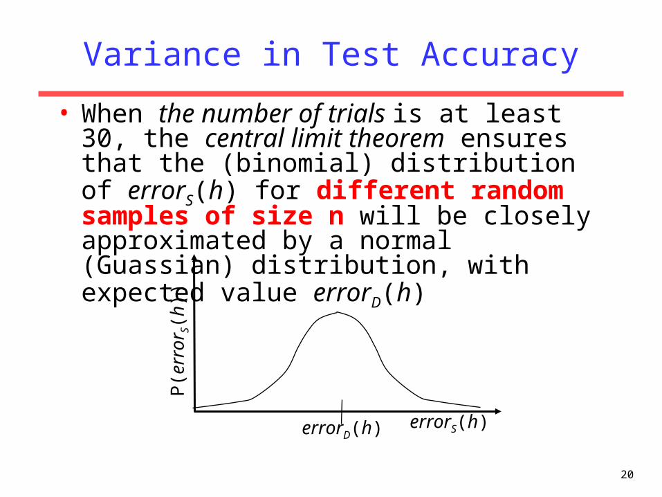
Variance in Test Accuracy

• When the number of trials is at least 30, the central limit theorem ensures that the (binomial) distribution of errorS(h) for different random samples of size n will be closely approximated by a normal (Guassian) distribution, with expected value errorD(h)

P(e

rror

S(h)

)

errorS(h)errorD(h)

Central Limit Theorem (μ=expected value of the true distribution)

21

In this experiment,each figure shows the distribution of values with a growing number of dices (from 1 to 50), and a large number of tosses.X axis is the sum of dices’ values when tossing n dices, and Y is the frequency of occurrence of that value

Summary

• Number of dicesnumber of examples to test

• Outcome of tossing n diceserrors of the classifier over n test examples

• The sample error errorS=r /n is a random variable following a Binomial distribution: if we repeat the experiment on different samples of the same dimension n we would obtain different values for errorSi with probability Pbinomial(ri /n )

• The expected value of errorS (for different experiments) equals np, where p is the real (unknown) error rate

• If the number of examples n is >30, then the underlying binomial distribution approximates a Gaussian distribution with same expected value

22

Confidence interval for an error estimate

• Confidence interval

• Provides a measure of the minimum and maximum expected discrepancy between the measured and real error rate

• Def: an N% confidence interval for an estimate e is an interval [LB,UB] that includes e with probability N% (with probability N% we have LBeUB)

• In our case, e= is a random variable representing the difference between true and estimated error (e is the error in estimating the error!!)

• If e obeys a gaussian distribution, the confidence interval can be easily estimated

23

Confidence interval

• Given an hypothesis h(x), if errorS(h(x)) obeys a gaussian with mean =errorD(h(x))=p and variance (which we said is approximately true for n>30) then the estimated value errorS(h(x)) on a sample S of n examples , r/n, with probability N% will lie in the following interval:

• zN is half of the lenght of the interval around μ that includes N% of the total probability mass

zN

Again, remember that theGaussian shows the probabilitydistribution of our outcomes(outcomes are the measured error values r/n)

Of course, we don’t knowwhere our estimator r/n is placedin this distribution, because we don’tactually know p nor , we only knowthat r/n lies somewhere in a gaussian-shaped distribution

Probability mass in a gaussian distribution

25

probability mass as a function of σ

probability mass as a function of ZN (with average 0 and standard deviation 1 )

So, what we actually KNOW is that WHEREVER our estimated error is in this Gaussian, it will be with 68% probability at a distance +-1 from the true error rate p, with 80% probability at a distance +-1.28 , with 98% probability at a distance +-2.33 , etc. And even though we don’t know , we have seen that it can be approximated with:

Finding the confidence interval

26

• N% of the mass lies between zN

• 80% lies in 1,28

• For a Gaussian with average 0 and standard deviation 1:

Finding the confidence interval

27

Calculating the N% Confidence Interval: Example

28

Example 2

29

Solution

30

Precision is 0.78 hence error rate r/n is 0.22; the test set has 50 instances, hence n=50

Choose e.g. to compute the N% confidence interval with N=0.95

One sided bound

31

a=(100-95)%=5% is the percentage of the gaussian areaoutside lower and upper extremes of the curve; a/2=2.5%a=(100-95)%=5% is the percentage of the gaussian areaoutside lower and upper extremes of the curve; a/2=2.5%

One sided two sided bounds

32

Upper bound

33

Evaluating error

• Evaluating the error rate of an hypothesis

• Evaluating alternative hypotheses

• Evaluating alternative learning algorithms

34

35

Comparing Two Learned Hypotheses

• When evaluating two hypotheses, their observed ordering with respect to accuracy may or may not reflect the ordering of their true accuracies.– Assume h1 is tested on test set S1 of size n1

– Assume h2 is tested on test set S2 of size n2

P(e

rror

S(h)

)

errorS(h)

errorS1(h1) errorS2(h2)

Observe h1 more accurate than h2

36

Comparing Two Learned Hypotheses

• When evaluating two hypotheses, their observed ordering with respect to accuracy may or may not reflect the ordering of their true accuracies.– Assume h1 is tested on test set S3 of size n1

– Assume h2 is tested on test set S4 of size n2

P(e

rror

S(h)

)

errorS(h)

errorS3(h1) errorS4(h2)

Observe h1 less accurate than h2

37

Z-Score Test for Comparing Learned Hypotheses

• Assumes h1 is tested on test set S1 of size n1 and h2 is tested on test set S2 of size n2.

• Compute the difference between the accuracy of h1 and h2

• Compute the standard deviation of the sample’s estimate of the difference.

2

22

1

11 ))(1()())(1()(2211

n

herrorherror

n

herrorherror SSSSd

Z-Score Test for Comparing Learned Hypotheses

• d^ ZNerrorS1(h1)(1-errorS1(h1))/n1 + errorS2(h2)(1-errorS2(h2))/n2 =d^ ZNσ

• Contrary to the previous case, where only one value of the difference was know (i.e. we did know the sample error, but not the true error) we now know both vales of the difference (both sample errors of the two hypotheses). Therefore, d is known, and d can be approximated, as before.

• We can then compute ZN

38

39

Z-Score Test for Comparing Learned Hypotheses (continued)

• Determine the confidence in the estimated difference by looking up the highest confidence, C, for the given z-score in a table.

confidencelevel

50% 68% 80% 90% 95% 98% 99%

z-score 0.67 1.00 1.28 1.64 1.96 2.33 2.58

40

Example

Assume we test two hypotheses on different test sets of size 100 and observe:

30.0)( 20.0)( 21 21 herrorherror SS

1.03.02.0)()( 21 21 herrorherrord SS

0608.0100

)3.01(3.0

100

)2.01(2.0

))(1()())(1()(

2

22

1

11 2211

n

herrorherror

n

herrorherror SSSSd

644.10608.0

1.0

d

dz

From table, if z=1.64 confidence level is 90%

confidencelevel

50% 68%

80%

90% 95% 98%

99%

z-score 0.67 1.00 1.28 1.64 1.96 2.33 2.58

41

Example 2

Assume we test two hypotheses on different test sets of size 100 and observe:

25.0)( 20.0)( 21 21 herrorherror SS

05.025.02.0)()( 21 21 herrorherrord SS

0589.0100

)25.01(25.0

100

)2.01(2.0

))(1()())(1()(

2

22

1

11 2211

n

herrorherror

n

herrorherror SSSSd

848.00589.0

05.0

d

dz

Confidence between 50% and 68%

confidencelevel

50% 68% 80% 90% 95% 98% 99%

z-score 0.67 1.00 1.28 1.64 1.96 2.33 2.58

42

Z-Score Test Assumptions: summary

• Hypotheses can be tested on different test sets; if same test set used, stronger conclusions might be warranted.

• Test set(s) must have at least 30 independently drawn examples (to apply central limit theorem).

• Hypotheses must be constructed from independent training sets.

• Only compares two specific hypotheses regardless of the methods used to construct them. Does not compare the underlying learning methods in general.

Evaluating error

• Evaluating the error rate of an hypothesis

• Evaluating alternative hypotheses

• Evaluating alternative learning algorithms

43

44

Comparing 2 Learning Algorithms

• Comparing the average accuracy of hypotheses produced by two different learning systems is more difficult since we need to average over multiple training sets. Ideally, we want to measure:

where LX(S) represents the hypothesis learned by learning algorithm LX from training data S.

• To accurately estimate this, we need to average over multiple, independent training and test sets.

• However, since labeled data is limited, generally must average over multiple splits of the overall data set into training and test sets (K-fold cross validation).

)))(())((( SLerrorSLerrorE BDADDS

K-fold cross validation of an hypothesis

45

Partition the test set in k equally sized random samples

K-fold cross validation (2)

46

At each step, learn from Li and test on Ti, then compute the error

Li Ti

e1

e2

e3

47

K-FOLD CROSS VALIDATION

48

K-Fold Cross Validation Comments

• Every example gets used as a test example once and as a training example k–1 times.

• All test sets are independent; however, training sets overlap significantly.

• Measures accuracy of hypothesis generated for [(k–1)/k]|D| training examples.

• Standard method is 10-fold.• If k is low, not sufficient number of train/test trials;

if k is high, test set is small and test variance is high and run time is increased.

• If k=|D|, method is called leave-one-out cross validation (at each step, you leave out one example).

49

Use K-Fold Cross Validation to evaluate different learners

Randomly partition data D into k disjoint equal-sized (N) subsets P1…Pk

For i from 1 to k do: Use Pi for the test set and remaining data for training Si = (D – Pi) hA = LA(Si) hB = LB(Si) δi = errorPi(hA) – errorPi(hB) Return the average difference in error:

t has the same role as zt has the same role as z

Error bound iscomputed as: Error bound iscomputed as:

50

Sample Experimental Results

SystemA SystemB

Trial 1 87% 82%

Trail 2 83% 78%

Trial 3 88% 83%

Trial 4 82% 77%

Trial 5 85% 80%

Average 85% 80%

Experiment 1

SystemA SystemB

Trial 1 90% 82%

Trail 2 93% 76%

Trial 3 80% 85%

Trial 4 85% 75%

Trial 5 77% 82%

Average 85% 80%

Experiment 2

Diff

+5%

+5%

+5%

+5%

+5%

+5%

Diff

+8%

+17%

–5%

+10%

– 5%

+5%

Which experiment provides better evidence that SystemA is better than SystemB?

Experiment 1 has σ=0, therefore we have a perfect confidence in the estimate of δExperiment 1 has σ=0, therefore we have a perfect confidence in the estimate of δ

51

Learning Curves

• Plots accuracy vs. size of training set.

• Has maximum accuracy (“Bayes optimal”) nearly been reached or will more examples help?

• Is one system better when training data is limited?

• Most learners eventually converge to Bayes optimal given sufficient training examples.

Tes

t Acc

urac

y

# Training examples

100%Bayes optimal

Random guessing

52

Noise Curves

• Plot accuracy versus noise level to determine relative resistance to noisy training data.

• Artificially add category or feature noise by randomly replacing some specified fraction of category or feature values with random values.

Tes

t Acc

urac

y

% noise added

100%

53

Experimental Evaluation Conclusions

• Good experimental methodology is important to evaluating learning methods.

• Important to test on a variety of domains to demonstrate a general bias that is useful for a variety of problems. Testing on 20+ data sets is common.

• Variety of freely available data sources– UCI Machine Learning Repository

http://www.ics.uci.edu/~mlearn/MLRepository.html– KDD Cup (large data sets for data mining)

http://www.kdnuggets.com/datasets/kddcup.html– CoNLL Shared Task (natural language problems)

http://www.ifarm.nl/signll/conll/

• Data for real problems is preferable to artificial problems to demonstrate a useful bias for real-world problems.

• Many available datasets have been subjected to significant feature engineering to make them learnable.