Embed Size (px)
Citation preview

1

<Insert Picture Here>
Best Practices for Extreme Performance with Data Warehousing on Oracle Database
Maria ColganSenior Principal Product Manager
3
<Insert Picture Here>
Agenda
• The three Ps of Data Warehousing– Power– Partitioning– Parallel
• Workload Management on a Data Warehouse

4
Best Practices for Data Warehousing3 Ps - Power, Partitioning, Parallelism
• Power – A Balanced Hardware Configuration– Weakest link defines the throughput
• Partition larger tables or fact tables– Facilitates data load, data elimination and join performance – Enables easier Information Lifecycle Management
• Parallel Execution should be used– Instead of one process doing all the work multiple processes
working concurrently on smaller units– Parallel degree should be power of 2
Goal is to minimize the amount of data accessed and use the most efficient joins

5
DiskArray 1
DiskArray 2
DiskArray 3
DiskArray 4
DiskArray 5
DiskArray 6
DiskArray 7
DiskArray 8
FC-Switch1 FC-Switch2H
BA
1
HB
A2
HB
A1
HB
A2
HB
A1
HB
A2
HB
A1
HB
A2
Balanced Configuration “The weakest link” defines the throughput
CPU Quantity and Speed dictate number of HBAs capacity of interconnect
HBA Quantity and Speed dictate number of Disk Controllers Speed and quantity of switches
Controllers Quantity and Speed dictatenumber of DisksSpeed and quantity of switches
Disk Quantity and Speed

6
Monitoring for a Balanced System• No Database Installed or running 10g or lower– Download Orion tool from Oracle.com– Run
• When Database is Installed– Run DBMS_RESOURCE_MANAGER.CALIBRATE_IO
./orion –run advanced –testname mytest –num_small 0 –size_large 1024 –type rand –simulate contact –write 0 –duration 60 –matrix column
SET SERVEROUTPUT ON
DECLARE
lat INTEGER; Iops INTEGER; Mbps INTEGER;
BEGIN
DBMS_RESOURCE_MANAGER.CALIBRATE_IO(<DISKS>,<MAX_LATENCY>,iops,mbps,lats);
DBMS_OUTPUT.PUT_LINE(‘Max_mbps = ‘|| mbps);
END;
/

7
<Insert Picture Here>
Agenda
• Data Warehousing Reference Architecture• The three Ps of Data Warehousing– Power– Partitioning– Parallel
• Workload Management on a Data Warehouse
8
Partitioning
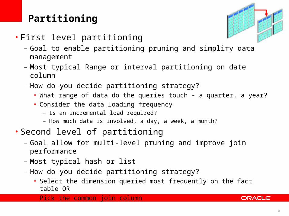
• First level partitioning– Goal to enable partitioning pruning and simplify data management– Most typical Range or interval partitioning on date column– How do you decide partitioning strategy?• What range of data do the queries touch - a quarter, a year?• Consider the data loading frequency
– Is an incremental load required? – How much data is involved, a day, a week, a month?
• Second level of partitioning– Goal allow for multi-level pruning and improve join performance – Most typical hash or list– How do you decide partitioning strategy?• Select the dimension queried most frequently on the fact table OR• Pick the common join column

9
Sales TableSales Table
SALES_Q3_199SALES_Q3_19988
SELECT sum(s.amount_sold)
FROM sales s
WHERE s.time_id BETWEEN
to_date(’01-JAN-1999’,’DD-MON-YYYY’)
AND
to_date(’01-JAN-2000’,’DD-MON-YYYY’);
Q: What was the total sales for the year
1999?
Partition Pruning
SALES_Q4_1998SALES_Q4_1998
SALES_Q1_1999SALES_Q1_1999
SALES_Q2_1999SALES_Q2_1999
SALES_Q3_1999SALES_Q3_1999
SALES_Q4_1999SALES_Q4_1999
SALES_Q1_2000SALES_Q1_2000

10
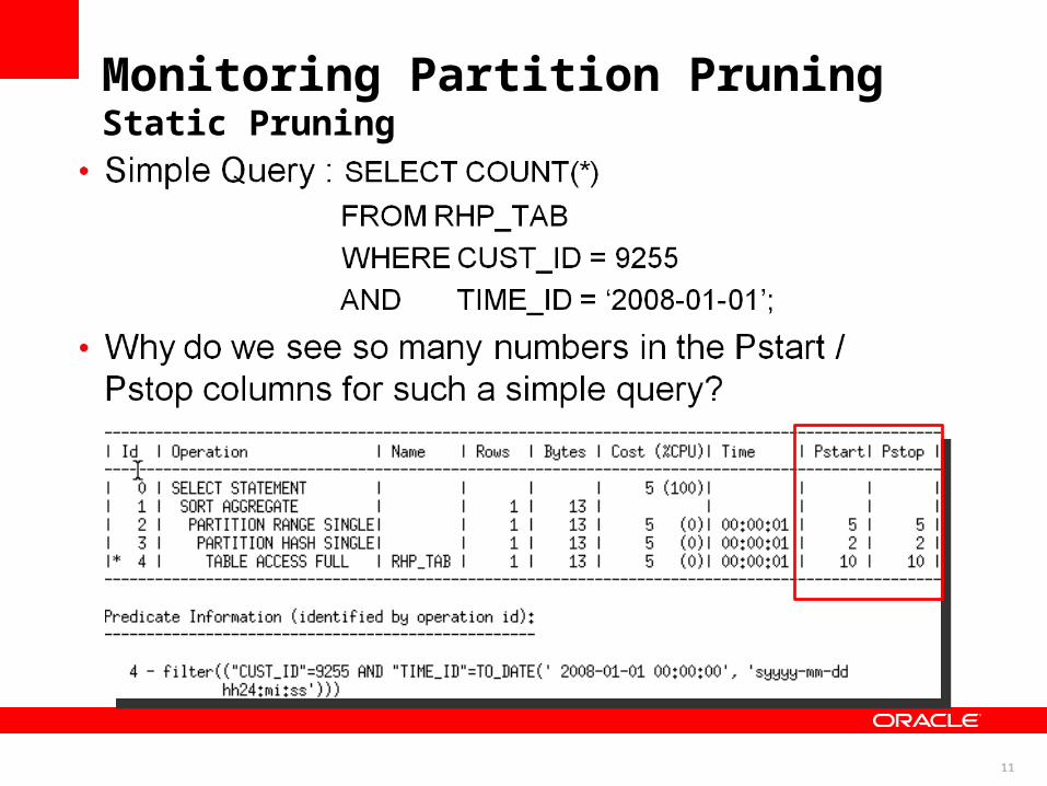
Monitoring Partition PruningStatic Pruning
• Sample plan
11
Monitoring Partition PruningStatic Pruning
12
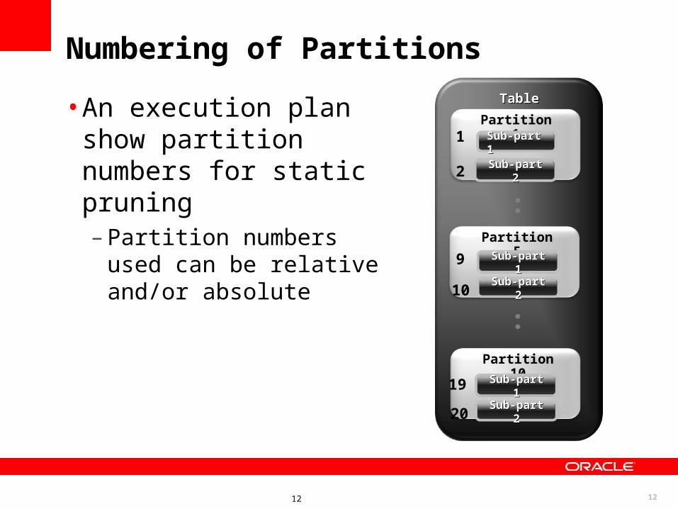
Numbering of Partitions
• An execution plan show partition numbers for static pruning– Partition numbers used can
be relative and/or absolute
12
TableTable
Partition 1
Partition 5
Partition 10
Sub-part 1Sub-part 1
Sub-part 2Sub-part 2
Sub-part 1Sub-part 1
Sub-part 2Sub-part 2
Sub-part 1Sub-part 1
Sub-part 2Sub-part 2
:
:
1
2
9
10
19
20

13
Monitoring Partition PruningStatic Pruning
Overall partition #
Overall partition #
range partition #
range partition #
Sub-partition #
Sub-partition #
14
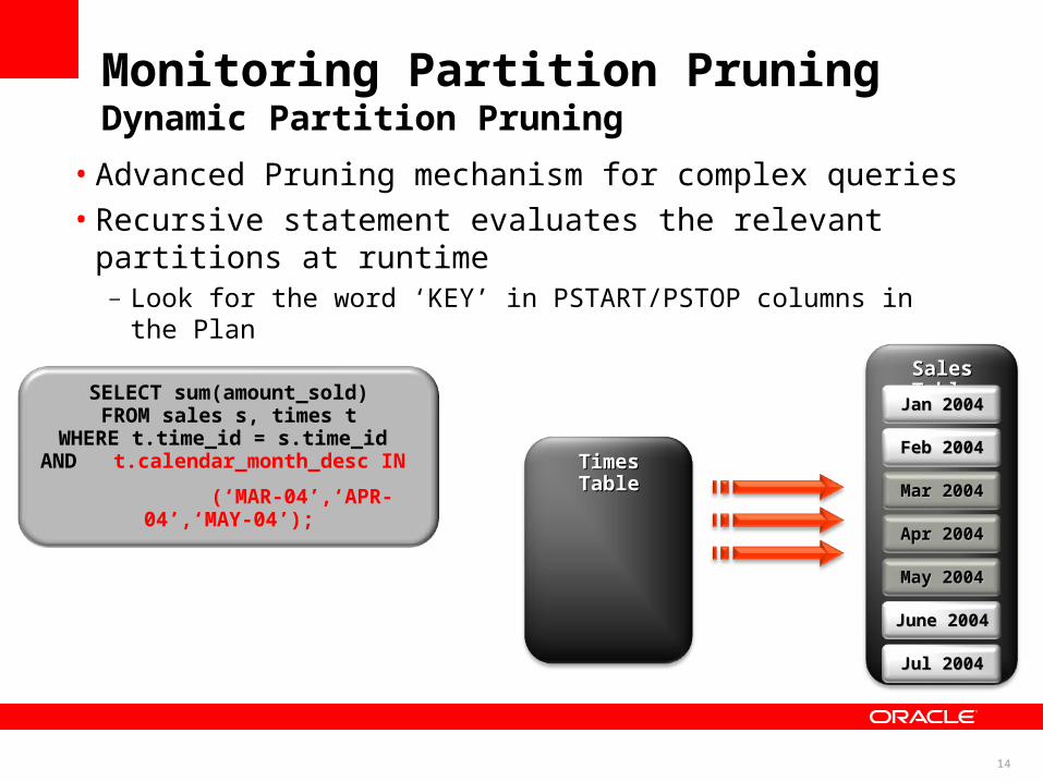
Monitoring Partition PruningDynamic Partition Pruning
• Advanced Pruning mechanism for complex queries• Recursive statement evaluates the relevant partitions at
runtime– Look for the word ‘KEY’ in PSTART/PSTOP columns in the Plan
SELECT sum(amount_sold)FROM sales s, times t
WHERE t.time_id = s.time_id AND t.calendar_month_desc IN
(‘MAR-04’,‘APR-04’,‘MAY-04’);
Sales TableSales Table
May 2004May 2004
June 2004June 2004
Jul 2004Jul 2004
Jan 2004Jan 2004
Feb 2004Feb 2004
Mar 2004Mar 2004
Apr 2004Apr 2004
Times TableTimes Table

15
Sample explain plan output
Monitoring Partition PruningDynamic Partition Pruning
• Sample plan
16
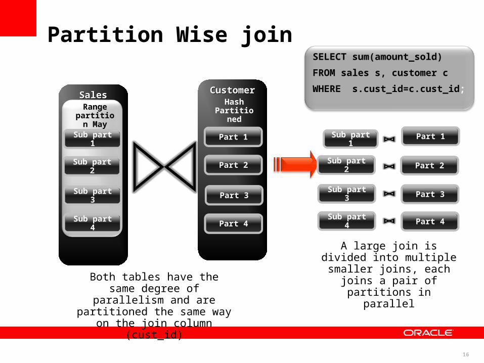
SELECT sum(amount_sold)
FROM sales s, customer c
WHERE s.cust_id=c.cust_id;
Both tables have the same degree of parallelism and are
partitioned the same way on the join column (cust_id)
SalesSalesRange
partition May 18th
2008
CustomerCustomerHash
Partitioned
Sub part 1
A large join is divided into multiple smaller joins, each joins a pair of partitions in
parallel
Part 1
Sub part 2
Sub part 3
Sub part 4
Part 2
Part 3
Part 4
Sub part 2
Sub part 3
Sub part 4
Sub part 1 Part 1
Part 2
Part 3
Part 4
Partition Wise join
17
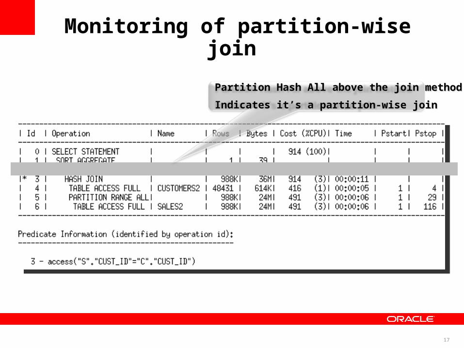
Monitoring of partition-wise join
Partition Hash All above the join methodPartition Hash All above the join method
Indicates it’s a partition-wise joinIndicates it’s a partition-wise join
18
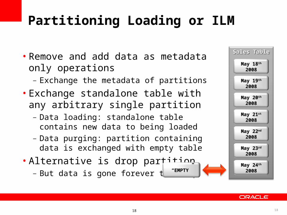
Partitioning Loading or ILM
• Remove and add data as metadata only operations– Exchange the metadata of partitions
• Exchange standalone table with any arbitrary single partition– Data loading: standalone table contains new data
to being loaded– Data purging: partition containing data is
exchanged with empty table
• Alternative is drop partition – But data is gone forever this way
18
Sales TableSales Table
May 22May 22ndnd 20082008
May 23May 23rdrd 20082008
May 24May 24thth 20082008
May 18May 18thth 20082008
May 19May 19thth 20082008
May 20May 20thth 20082008
May 21May 21stst 20082008
““EMPTY”EMPTY”

19
Sales TableSales Table
May 22May 22ndnd 20082008
May 23May 23rdrd 20082008
May 24May 24thth 2008 2008
May 18May 18thth 2008 2008
May 19May 19thth 2008 2008
May 20May 20thth 2008 2008
May 21May 21stst 2008 2008
DBA
1. Create external table for flat files
2. Use CTAS command to create non-partitioned table TMP_SALES
Tmp_ sales Tmp_ sales TableTable
4. Alter table Sales exchange partition May_24_2008 with table tmp_sales
May 24May 24thth 20082008
Sales table now has all the data
3. Create indexes
Tmp_ sales Tmp_ sales TableTable
Partition Exchange Loading
5. Gather Statistics

20
Incremental Global Statistics
Sales TableSales Table
May 22May 22ndnd 20082008
May 23May 23rdrd 20082008
May 18May 18thth 20082008
May 19May 19thth 20082008
May 20May 20thth 20082008
May 21May 21stst 20082008
Sysaux Tablespace
S1
S2
S3
S4
S5
S6
1. Partition level stats are gathered & synopsis
created
Global Statistic
2. Global stats generated by aggregating partition
synopsis

21
Incremental Global Statistics Cont’d
Sales TableSales Table
May 22May 22ndnd 20082008
May 23May 23rdrd 20082008
May 24May 24thth 20082008
May 18May 18thth 20082008
May 19May 19thth 20082008
May 20May 20thth 20082008
May 21May 21stst 20082008
Sysaux Tablespace
3. A new partition is added to the table & Data is
Loaded
May 24May 24thth 20082008
S7 4. Gather partition statistics for new
partition
S1
S2
S3
S4
S5
S6
5. Retrieve synopsis for each of the other
partitions from Sysaux
Global Statistic
6. Global stats generated by aggregating the original
partition synopsis with the new one

22
Things to keep in mind when using partition
• Partition pruning on hash partitions only works for equality or in-list where clause predicates• Partition pruning on multi-column hash partitioning
only works if there is a predicate on all columns used• To get a partition-wise join when using parallel query
make sure the DOP is equal to or a multiple of the number of partitions• If you load data into a new partition every day and
users immediately start querying it, copy the statistics from the previous partition until you have time to gather stats (DBMS_STATS.COPY_TABLE_STATS)
23
<Insert Picture Here>
Agenda
• Data Warehousing Reference Architecture• The three Ps of Data Warehousing– Power– Partitioning– Parallel
• Workload Management on a Data Warehouse
24
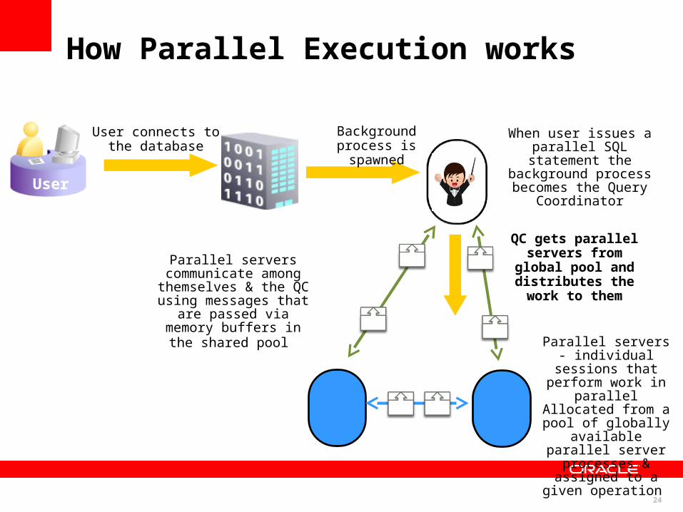
How Parallel Execution works
User connects to the database
User
Background process is spawned
When user issues a parallel SQL statement the
background process becomes the Query
Coordinator
QC gets parallel servers from global pool and distributes
the work to them
Parallel servers - individual sessions that perform work in parallel Allocated from a pool of
globally available parallel server
processes & assigned to a given operation
Parallel servers communicate among
themselves & the QC using messages that are passed via memory buffers in the
shared pool
25
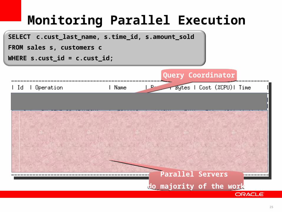
Parallel Servers
do majority of the work
Parallel Servers
do majority of the work
Monitoring Parallel ExecutionSELECT c.cust_last_name, s.time_id, s.amount_sold
FROM sales s, customers c
WHERE s.cust_id = c.cust_id;
Query CoordinatorQuery Coordinator
26
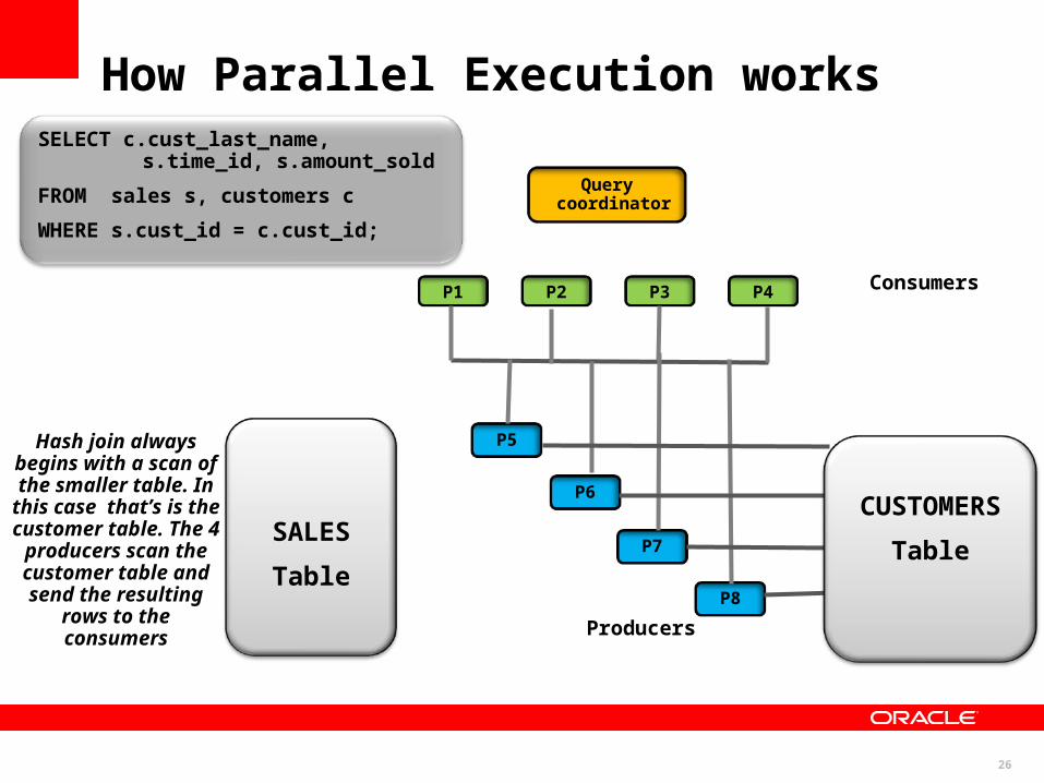
Producers
Consumers
Query coordinator
P1 P2 P3 P4
Hash join always begins with a scan of the smaller table. In this case that’s is the customer table.
The 4 producers scan the customer table
and send the resulting rows to the
consumers
P8
P7
P6
P5
SALES
Table
CUSTOMERS
Table
SELECT c.cust_last_name, s.time_id, s.amount_sold
FROM sales s, customers c
WHERE s.cust_id = c.cust_id;
How Parallel Execution works

27
Producers
Consumers
Query coordinator
P1 P2 P3 P4
Once the 4 producers finish scanning the customer table, they
start to scan the Sales table and send the resulting rows to
the consumersP8
P7
P6
P5
SALES
Table
CUSTOMERS
Table
SELECT c.cust_last_name, s.time_id, s.amount_sold
FROM sales s, customers c
WHERE s.cust_id = c.cust_id;
How Parallel Execution works
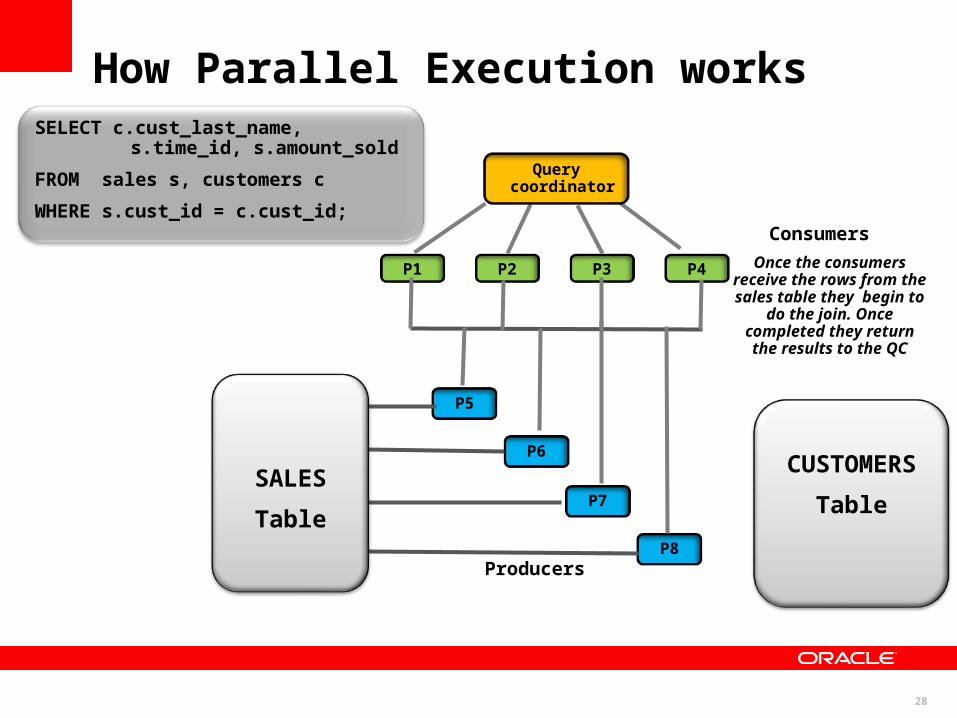
28
Producers
Consumers
P1 P2 P3 P4
P8
P7
P6
P5
Once the consumers receive the rows from the sales table they begin to
do the join. Once completed they return the results to the QC
Query coordinator
SALES
Table
CUSTOMERS
Table
SELECT c.cust_last_name, s.time_id, s.amount_sold
FROM sales s, customers c
WHERE s.cust_id = c.cust_id;
How Parallel Execution works
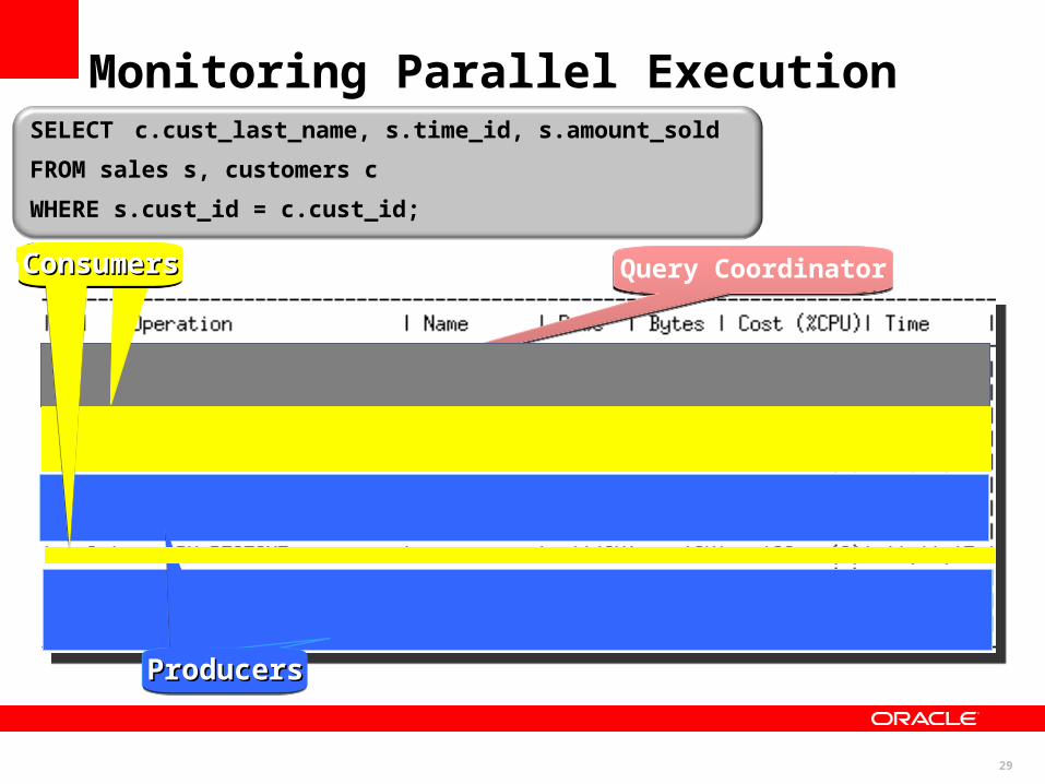
29
SELECT c.cust_last_name, s.time_id, s.amount_sold
FROM sales s, customers c
WHERE s.cust_id = c.cust_id;
Query CoordinatorQuery Coordinator
ProducersProducersProducersProducersProducersProducers
ConsumersConsumersConsumersConsumersConsumersConsumers
Monitoring Parallel Execution

30
Best Practices for using Parallel Execution
Current Issues• Difficult to determine ideal DOP for each table without manual tuning• One DOP does not fit all queries touching an object• Not enough PX server processes can result in statement running serial• Too many PX server processes can thrash the system• Only uses IO resources
Solution
• Oracle automatically decides if a statement
–Executes in parallel or not and what DOP it will use
–Can execute immediately or will be queued
–Will take advantage of aggregated cluster memory or not

31
Auto Degree of Parallelism
Enhancement addressing:• Difficult to determine ideal DOP for each table without manual tuning• One DOP does not fit all queries touching an object
SQLstatement
Statement is hard parsedAnd optimizer determines
the execution plan
Statement executes in parallel
Actual DOP = MIN(PARALLEL_DEGREE_LIMIT, ideal DOP)
Statement executes serially
If estimated time less than threshold*
Optimizer determines ideal DOP based on all scan operations
If estimated time greater than threshold*
* Threshold set in parallel_min_time_threshold (default = 10s)
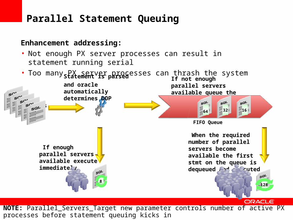
SQLstatements
Statement is parsed
and oracle automatically determines DOP
If enough parallel servers available execute immediately
If not enough parallel servers available queue the statement
128163264
8
FIFO Queue
When the required number of parallel servers become available the first stmt on the queue is dequeued and executed
128
163264
Parallel Statement Queuing
Enhancement addressing:• Not enough PX server processes can result in statement running serial• Too many PX server processes can thrash the system
NOTE: Parallel_Servers_Target new parameter controls number of active PX processes before statement queuing kicks in

Simple Example of Queuing
8 Statements run before queuing kicks in
Queued stmts are indicated by the clock
34
<Insert Picture Here>
Agenda
• Data Warehousing Reference Architecture• The three Ps of Data Warehousing– Power– Partitioning– Parallel
• Workload Management on a Data Warehouse
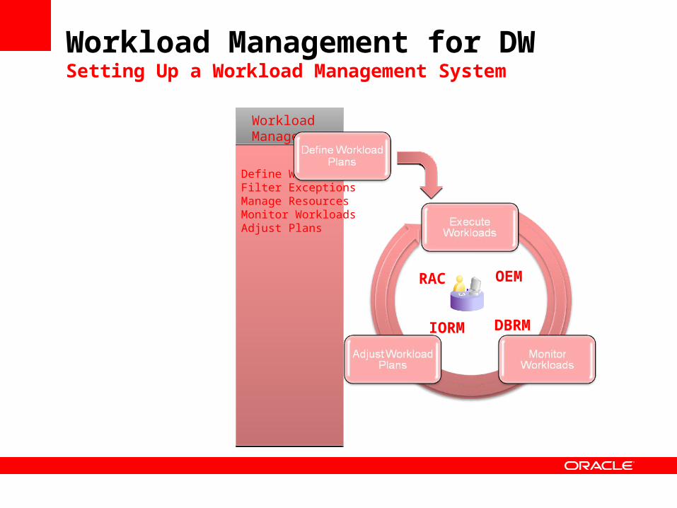
Workload Management for DWSetting Up a Workload Management System
WorkloadManagement
Define WorkloadsFilter ExceptionsManage ResourcesMonitor WorkloadsAdjust Plans
IORM
RAC OEM
DBRM

Workload Management for DWOracle Database Resource Manager
• Traditionally you were told to use Resource Management if data warehouse is CPU bound
• Protects critical tasks from interference from non-critical tasks• Allows CPU to be utilized according to a specific ratio• Prevents thrashing and system instability that can occur with
excessive CPU loads
• But did you know Resource Manager can• Control DOP for each group of users• Control the number of concurrent queries for each group• Prevent runaway queries
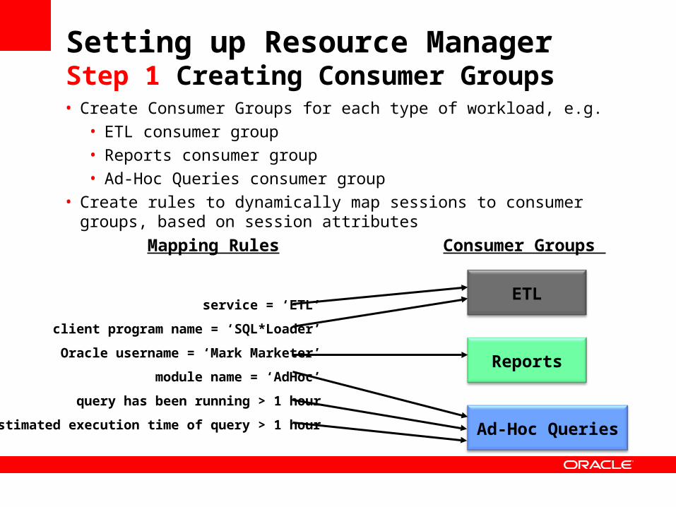
Setting up Resource Manager Step 1 Creating Consumer Groups• Create Consumer Groups for each type of workload, e.g.
• ETL consumer group
• Reports consumer group
• Ad-Hoc Queries consumer group
• Create rules to dynamically map sessions to consumer groups, based on session attributes
ETL
Reports
Ad-Hoc Queries
service = ‘ETL’
client program name = ‘SQL*Loader’
Oracle username = ‘Mark Marketer’
module name = ‘AdHoc’
query has been running > 1 hour
estimated execution time of query > 1 hour
Mapping Rules Consumer Groups
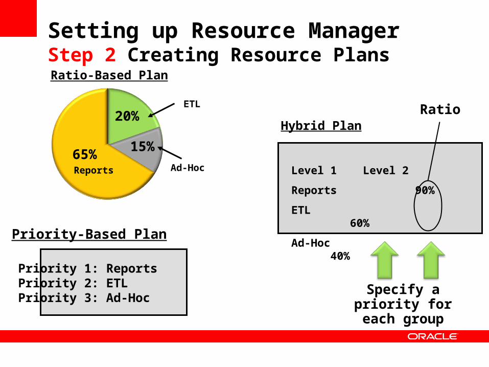
Setting up Resource Manager Step 2 Creating Resource Plans
Ratio-Based Plan
Priority 1: ReportsPriority 2: ETLPriority 3: Ad-Hoc
Level 1 Level 2
Reports 90%
ETL 60%
Ad-Hoc 40%
Specify a priority for each group
Ratio
65%
20%
15%
Ad-Hoc
ETL
Reports
Priority-Based Plan
Hybrid Plan
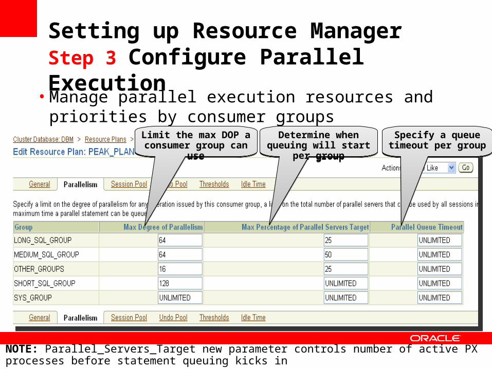
Setting up Resource Manager Step 3 Configure Parallel Execution
• Manage parallel execution resources and priorities by consumer groups
Limit the max DOP a consumer group can
use
Limit the max DOP a consumer group can
use
Determine when queuing will start per
group
Determine when queuing will start per
group
Specify a queue timeout per groupSpecify a queue
timeout per group
NOTE: Parallel_Servers_Target new parameter controls number of active PX processes before statement queuing kicks in
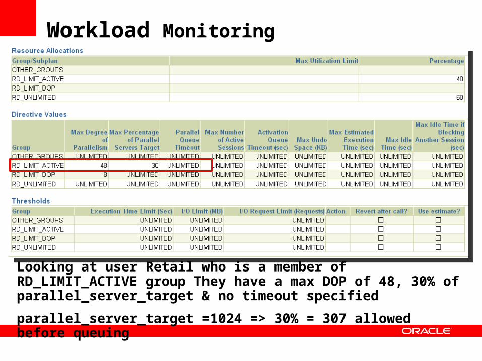
Workload Monitoring
Looking at user Retail who is a member of RD_LIMIT_ACTIVE group They have a max DOP of 48, 30% of parallel_server_target & no timeout specified
parallel_server_target =1024 => 30% = 307 allowed before queuing

Workload Monitoring
DOP Limited to 48
DOP Limited to 48
Only 3 sessions allowed to run before queue
Only 3 sessions allowed to run before queue
3 X 48 = 144 not 307 so why are stmts being queued?
3 X 48 = 144 not 307 so why are stmts being queued?
Remaining stmts are queued until PX resources are freed up
Remaining stmts are queued until PX resources are freed up
Statements require two sets of PX process for producers & consumers

Resource Manager - Statement Queuing
Request
Assign
Static Reports
Tactical Queries
Ad-hocWorkload
Queue
Queue
Queue25%
25%
50%
256
256
512
• Queuing is embedded with DBRM• One queue per consumer group
<Insert Picture Here>
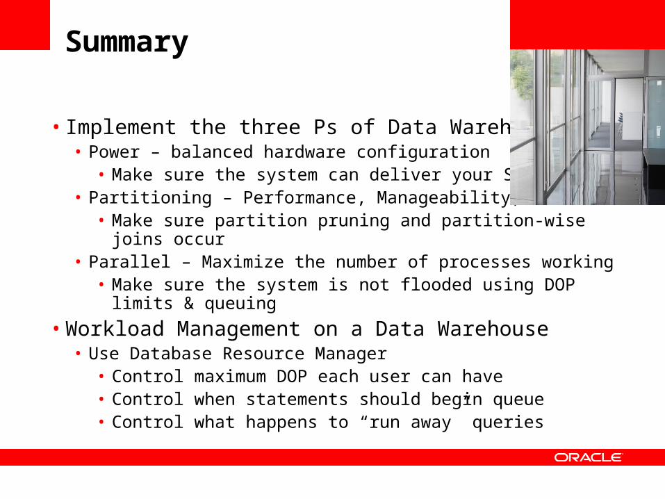
Summary
• Implement the three Ps of Data Warehousing• Power – balanced hardware configuration
• Make sure the system can deliver your SLA• Partitioning – Performance, Manageability, ILM
• Make sure partition pruning and partition-wise joins occur • Parallel – Maximize the number of processes working
• Make sure the system is not flooded using DOP limits & queuing
• Workload Management on a Data Warehouse• Use Database Resource Manager
• Control maximum DOP each user can have• Control when statements should begin queue• Control what happens to “run away” queries

44
Q & A
45
The preceding is intended to outline our general product direction. It is intended for information purposes only, and may not be incorporated into any contract. It is not a commitment to deliver any material, code, or functionality, and should not be relied upon in making purchasing decisions.The development, release, and timing of any features or functionality described for Oracle’s products remains at the sole discretion of Oracle.