1

Aggregate Expenditure Components

CHAPTER

9

© 2003 South-Western/Thomson Learning

2

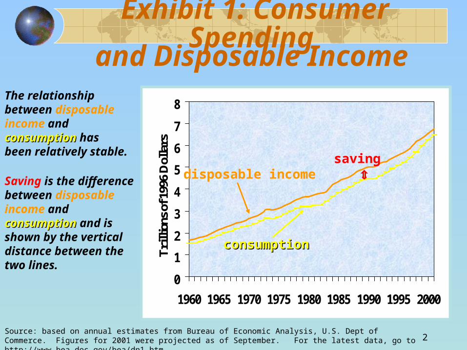
Exhibit 1: Consumer Spending

The relationship between disposable income and consumptionconsumption has been relatively stable.

Saving is the difference between disposable income and consumptionconsumption and is shown by the vertical distance between the two lines.

and Disposable Income

0

1

2

3

4

5

6

7

8

1960 1965 1970 1975 1980 1985 1990 1995 2000

Trill

ions

of 1

996

Dol

lars

consumptionconsumption

disposable incomesaving

Source: based on annual estimates from Bureau of Economic Analysis, U.S. Dept of Commerce. Figures for 2001 were projected as of September. For the latest data, go to http://www.bea.doc.gov/bea/dn1.htm.

3

Exhibit 2: Dependence of Consumer Spending on Disposable Income

There is a clear and direct relationship between consumption and disposable income.

012345678

0 1 2 3 4 5 6 7Real Disposable Income

Rea

l Con

sum

er S

pen

din

g

Source: based on estimates from the Bureau of Economic Analysis, U.S. Dept of Commerce. Point for 2001 was projected as of September. For the latest data, go to http://www.bea.doc.gov/bea/dn1.htm.

1970

1986

1995

2001

4

Exhibit 3: The Consumption Function

Both disposable income and consumption are measured in real terms, or in inflation-adjusted dollars .

0123456789

10

1 2 3 4 5 6 7 8 9Real Disposable Income

(trillions of dollars)

Rea

l C

on

sum

pti

on

(tr

illi

ons

of

do

llars

)

5

Marginal Propensities to Consume and Save

What happens to consumption and saving when income changes?

Marginal Propensity to Consume, MPC equals the change in consumption divided by the change in incomeMarginal Propensity to Save, MPS equals the change in saving divided by the change in income

MPC + MPS = 1This equality exists because all disposable income must either be spent on consumption or saved

6

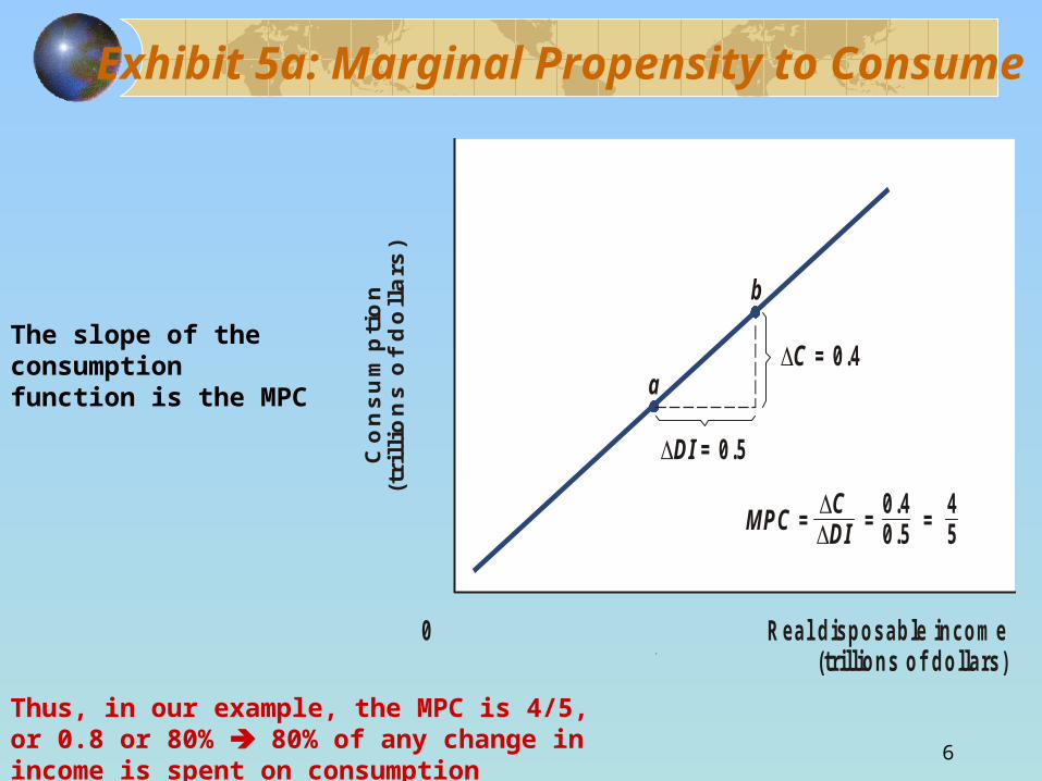
Exhibit 5a: Marginal Propensity to Consume

Real disposable income (trillions of dollars)

a

b

0

C = 0.4

DI = 0.5

0.4 4 0.5 5MPC = = =

C DI

Co

ns

um

pti

on

(t

rill

ion

s o

f d

olla

rs)

The slope of the consumption function is the MPC

Thus, in our example, the MPC is 4/5, or 0.8 or 80% 80% of any change in income is spent on consumption

7

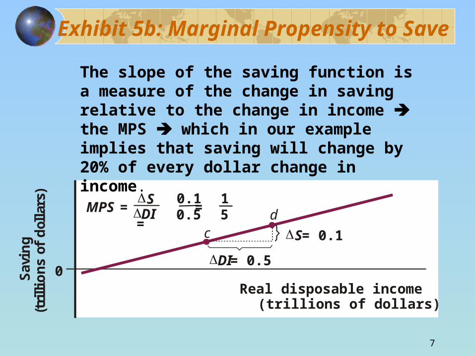
Exhibit 5b: Marginal Propensity to Save

cd

0Real disposable income

(trillions of dollars)

DI = 0.5

S = 0.1

MPS = = =S DI

Sav

ing

(t

rilli

on

s o

f d

olla

rs)

0.10.5

15

The slope of the saving function is a measure of the change in saving relative to the change in income the MPS which in our example implies that saving will change by 20% of every dollar change in income.

8

Nonincome DeterminantsAlong a given consumption function, consumer spending depends on the level of disposable income in the economy, other things constantWhat are these factors that could cause the entire consumption function to shift?

Net WealthPrice LevelInterest RateExpectations

9

Net Wealth

Net wealth is the value of all assets that households own minus any liabilities, or debts owed

A decrease in net wealth would make consumers less inclined to spend – more inclined to save

10

Price LevelSome household wealth is held in dollar-denominated assets such as bank accounts and cash

Whenever the price level changes, the real value of these dollar-denominated financial assets changes

Increase in the price level reduces the purchasing power of wealth held in fixed dollar assets households consume less and save moreDecreases in the price level increase the purchasing power of wealth held in fixed assets households consume more and save less

11

Interest Rate

InterestThe reward savers earn for deferring consumption and, the cost paid by borrowers for current spending power

The higher the interest ratehigher the interest rate, the less is spent on items purchased on credit households save more and borrow less consumption function shifts downward

12

ExpectationsExpectations influence economic behavior in a variety of ways

Changing expectations about price levels, interest rates, job security and other such factors influence consumer behavior

If expectations become more pessimistic consumption function shifts downward

If expectations become more optimistic consumption function shifts upward

13

InvestmentInvestment consists of spending on

New factories and new equipmentNew housingNet change in inventories

Firms invest in capital goods now in the expectation of a future return

The expected rate of return equals the annual dollar earnings expected from the investment divided by the purchase price

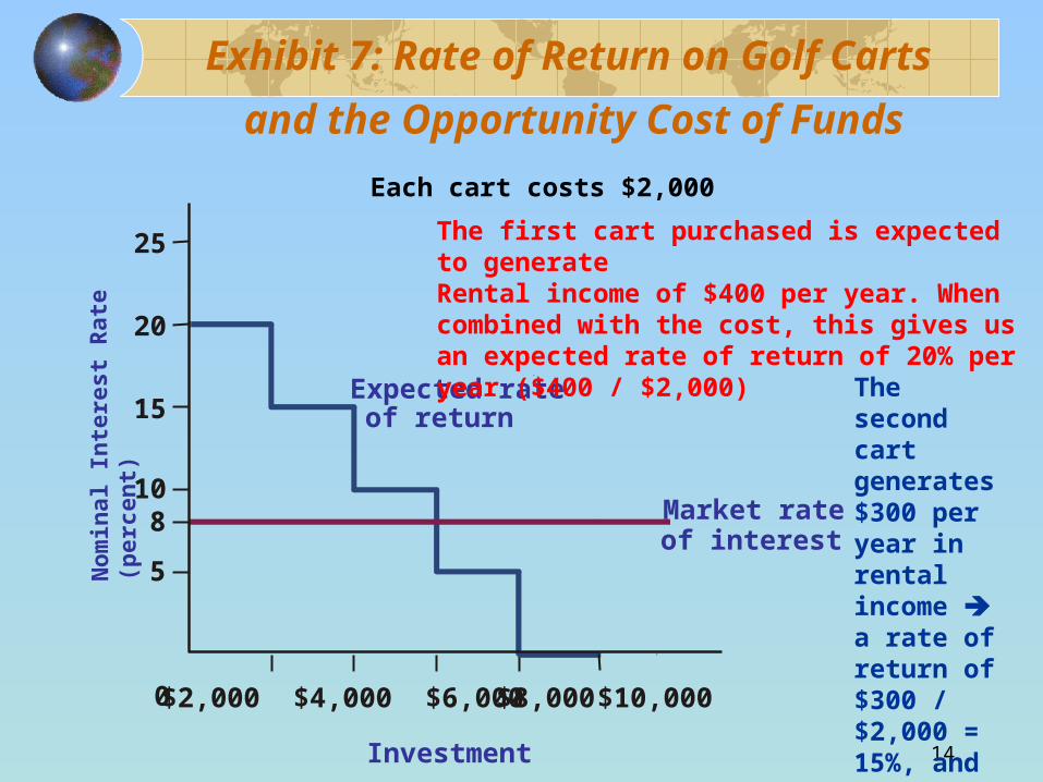
14

Exhibit 7: Rate of Return on Golf Carts

and the Opportunity Cost of Funds

$2,000 $4,000 $6,000 $10,000

25

20

15

10

5

Expected rate of return

0

8 Market rate of interest

$8,000

Each cart costs $2,000

The first cart purchased is expected to generateRental income of $400 per year. When combined with the cost, this gives us an expected rate of return of 20% per year ($400 / $2,000)

The second cart generates $300 per year in rental income a rate of return of $300 / $2,000 = 15%, and so on .

Investment

No

min

al In

tere

st R

ate

(per

cen

t)

15

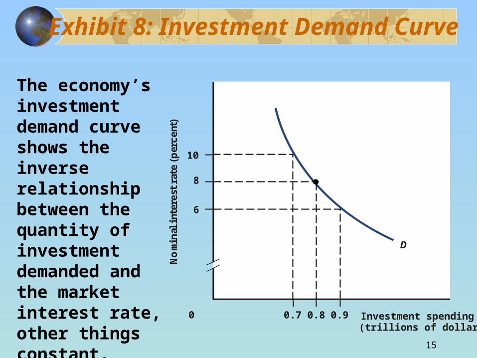
Exhibit 8: Investment Demand Curve

D

0

8

6

10

Investment spending (trillions of dollars)

No

min

al i

nte

rest

rat

e (p

erc

ent)

0.7 0.90.8

The economy’s investment demand curve shows the inverse relationship between the quantity of investment demanded and the market interest rate, other things constant.

16

Planned Investment and Income

Investment depends more on interest rates and on business expectations than on the prevailing level of income

One reason for this is that some investments take years to completeAdditionally, investment, once in place, is expected to last for years

Thus, the investment decision is said to be “forward looking,” based more on expected profit than on current levels of income and output

17

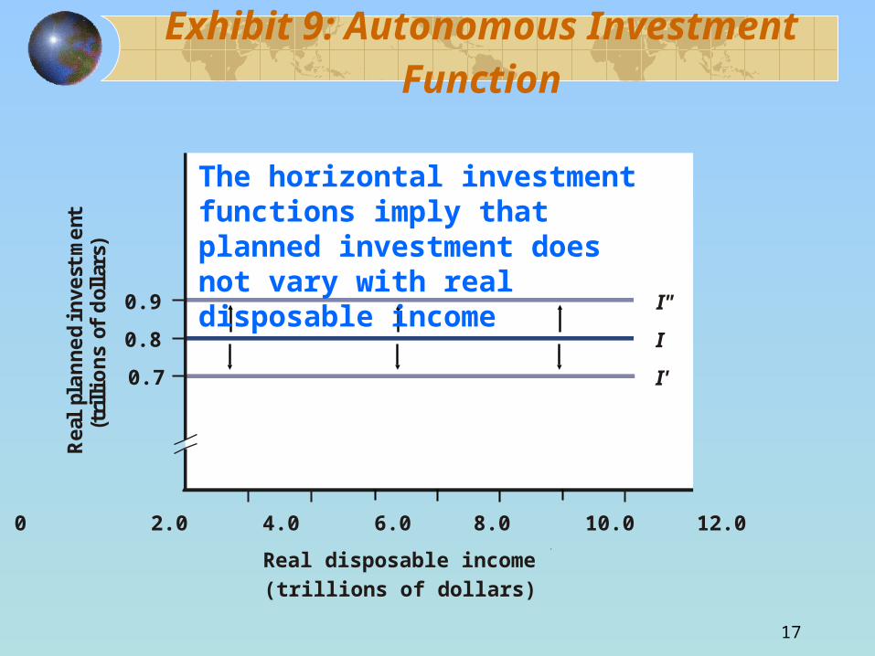
Exhibit 9: Autonomous Investment FunctionR

ea

l p

lan

ne

d i

nv

es

tme

nt

(tri

llio

ns

of

do

lla

rs)

0.8

0 2.0 4.0 6.0 8.0 10.0 12.0

Real disposable income

(trillions of dollars)

I

0.9 I"

0.7 I'

The horizontal investment functions imply that planned investment does not vary with real disposable income

18

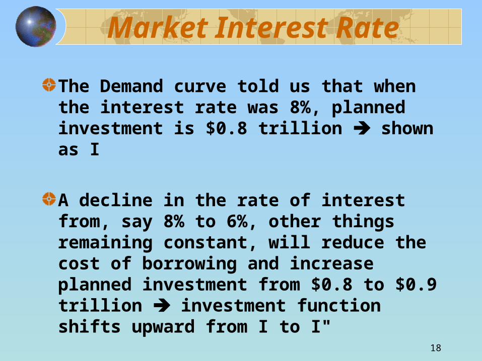
Market Interest Rate

The Demand curve told us that when the interest rate was 8%, planned investment is $0.8 trillion shown as I

A decline in the rate of interest from, say 8% to 6%, other things remaining constant, will reduce the cost of borrowing and increase planned investment from $0.8 to $0.9 trillion investment function shifts upward from I to I"

19

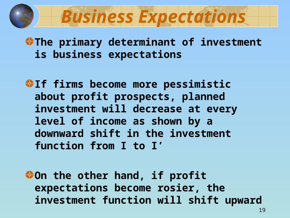
Business ExpectationsThe primary determinant of investment is business expectations

If firms become more pessimistic about profit prospects, planned investment will decrease at every level of income as shown by a downward shift in the investment function from I to I’

On the other hand, if profit expectations become rosier, the investment function will shift upward

20For the latest data, go to http://www.bea.gov

Exhibit 10: Annual Percentage Change in US Real GDP, Consumption, and Investment

21

Government Purchase Function

Government purchases in 2001 accounted for about 18% of GDP

One-third of the total was by the federal governmentTwo-thirds by state and local governments

The government purchase function relates government purchases to the level of income in the economy, other things constant

22

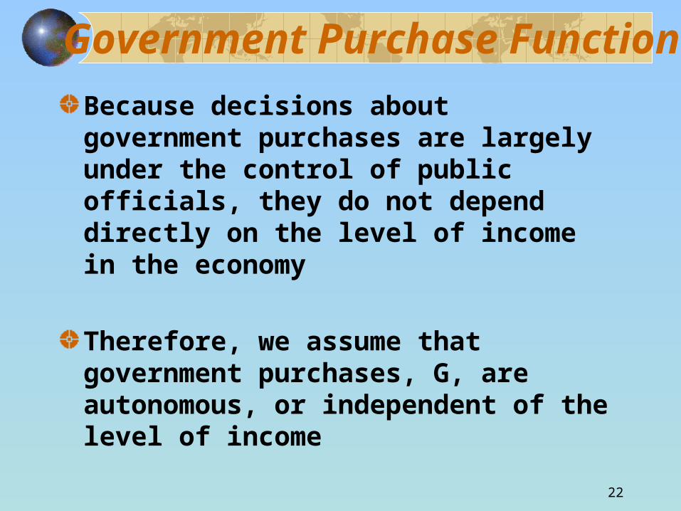
Government Purchase Function

Because decisions about government purchases are largely under the control of public officials, they do not depend directly on the level of income in the economy

Therefore, we assume that government purchases, G, are autonomous, or independent of the level of income

23

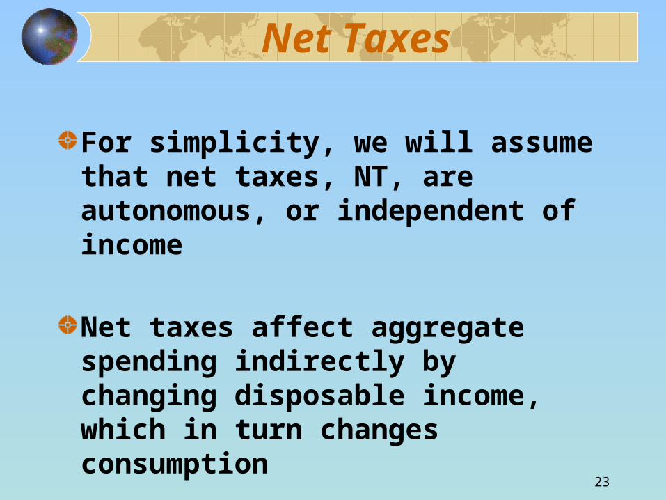
Net Taxes

For simplicity, we will assume that net taxes, NT, are autonomous, or independent of income

Net taxes affect aggregate spending indirectly by changing disposable income, which in turn changes consumption

24

Net Exports

The rest of the world affects aggregate expenditure through imports and exports

The United States, with only one-twentieth of the world’s population – accounts for about one-sixth of the world’s imports and one-eighth of the world’s exports

25

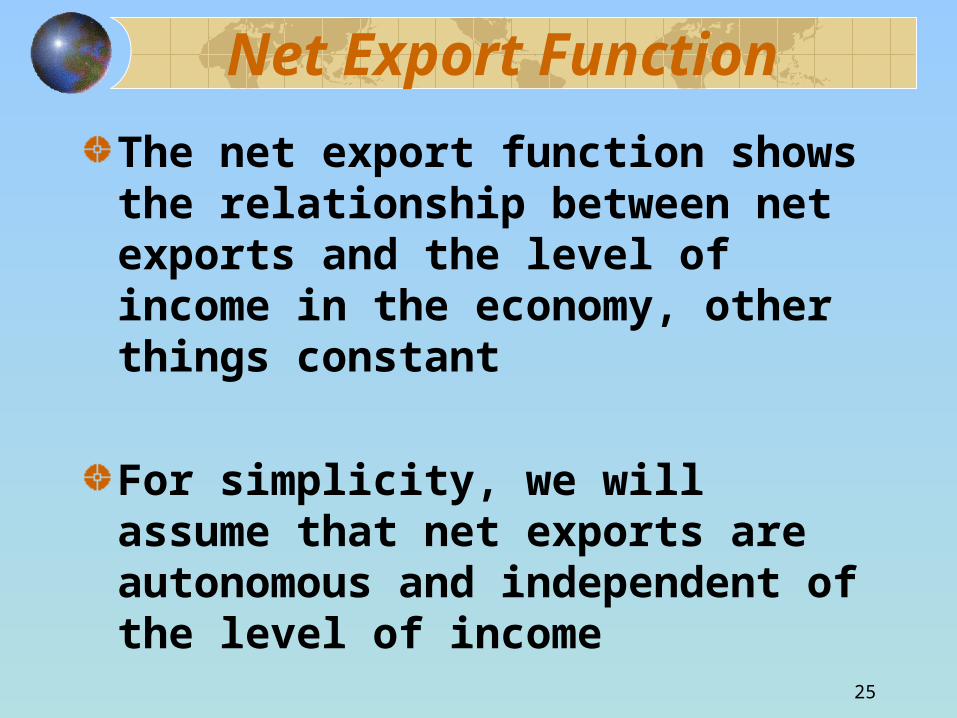
Net Export Function

The net export function shows the relationship between net exports and the level of income in the economy, other things constant

For simplicity, we will assume that net exports are autonomous and independent of the level of income

26

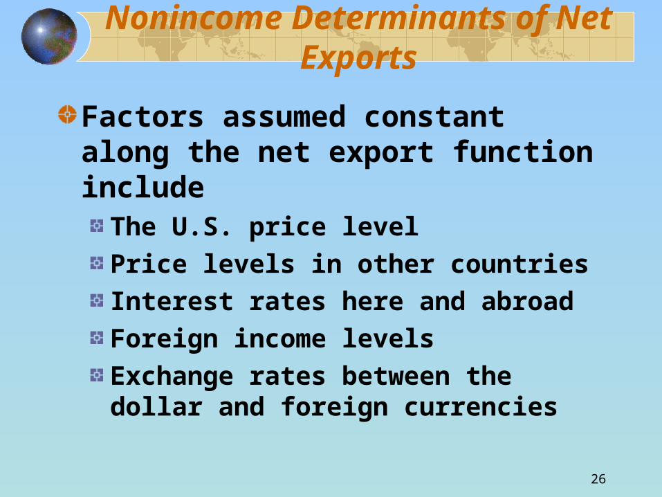
Nonincome Determinants of Net Exports

Factors assumed constant along the net export function include

The U.S. price levelPrice levels in other countriesInterest rates here and abroadForeign income levelsExchange rates between the dollar and foreign currencies

27

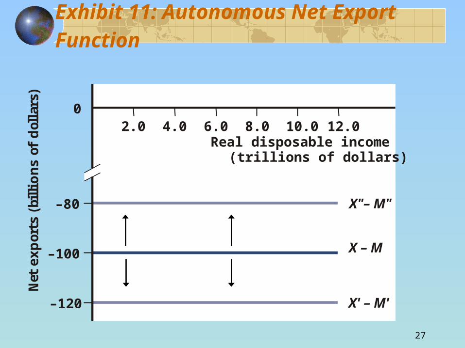
Exhibit 11: Autonomous Net Export Function

–80

–100

–120

0

Ne

t e

xp

ort

s (b

illi

on

s o

f d

oll

ars

)

X"– M"

X – M

X' – M'

2.0 4.0 6.0 8.0 10.0 12.0Real disposable income

(trillions of dollars)