1

Aggregate R&D Expenditure

and Endogenous Economic Growth*

Mª Jesús Freire-Serén**

Universitat Autònoma de Barcelonaand

Universidade de Vigo

Feb. 1999

WP 436.99

JEL Classification: O30, O40, O47.Keywords : Technological change, endogenous growth, aggregateR&D-expenditure, empiricalevidence.

* I am indebted to Angel de la Fuente, Jaime Alonso and Lorenzo Serrano for their very helpfuldiscussions and comments. Of course, all errors that remain are entirely my own. Financialsupport from DGICYT grant PB95-130 is gratefully acknowlwedge.** Mailing address: M. Jesús Freire-Serén, Universidade de Vigo, Facultade de CienciasEconómicas, Lagoas, Marcosende s/n, 36200 Vigo (Pontevedra), Spain. Phone: +34986812524. Fax:+34986812401. E-Mail: mjfreire@uvigo.es.

2

Resumen

El objetivo de este trabajo es analizar teórica y empíricamente el papel que juega el gasto

agregado en actividades de I+D en el crecimiento económico. Para ello, se propone una tecnología

de innovación definida en unidades de gasto. De este modo se obtiene crecimiento endógeno

sostenido aunque no exista crecimiento de la población. Esto nos permite analizar el efecto de

ciertas políticas fiscales. Para la estimación econométrica utilizaremos una especificación

obtenida directamente del modelo teórico. Más en concreto, dicha especificación se obtiene a

partir de la condición de libre entrada del sector de innovacion y de la solución de la ecuacion

dinámica que describe la evolución del precio de las patentes.

Abstract

The aim of this paper is to theoretically and empirically analyze the role that aggregate R&D-

expenditures play in economic growth. We introduce a technology of innovation based on R&D-

expenditures instead of labor to see how this consideration generates sustainable growth

determined endogenously, even if population growth does not exist. Therefore, it seems relevant

to analyze the effects of different fiscal policies. For the empirical analysis we make use of an

econometric model obtained from the decentralized equilibrium. More precisely, the

specification is obtained using the free-entry condition that the competitive equilibrium states

for the R&D-activity and the policy function defining the dynamic evolution of patentees' price.

3

1. Introduction.

This paper presents an R&D-based model of economic growth in the line of those proposed

by Romer (1990), Grossman-Helpman (1991) and Aghion-Howitt (1992). In this type of models

the research and development efforts made by profit-maximizing agents are the basis for

technological advance, which underlies sustained growth. Moreover, these models adopt some

kind of monopolistic power to generate a surplus that can be assigned to the innovation activity.

In particular, this activity creates non-rival ideas that are used in the form of patents to produce

new capital goods by monopolistic firms. Finally, these goods will be complementary inputs in

the production of consumption goods. In this way, the introduction of new capital goods does not

reduce the marginal productivity of the pre-existing ones, and so the innovation activity

generates perpetual growth through the increase in the number of capital goods.

The aim of the paper is to theoretically and empirically analyze the role that aggregate

R&D-expenditures play in the growth of per capita income. Generally, the R&D-based growth

models consider an R&D technology that uses (skilled) labor as the unique input, so that the

quantity and the quality of labor determines the production of R&D, and therefore the growth

rate of the economy. We instead are interested in analyzing the effects of expenditures in this

activity, i.e., we investigate whether the income that individuals devoted to finance the

innovation activity translates into a growth of per capita income. Actually, the innovation

process is intensive in human capital. However, we are interested in analyzing the private

choice of investing income in this process. The economy must channel the individuals' savings to

finance the R&D-activity. The question is what are the determinants of this decision.

Therefore, by R&D-expenditure we understand the income devoted to finance the total cost of

the R&D-activity, i.e., wages, infrastructure, capital and so on used in the innovative process.

In the present model, the endogenous accumulation of wealth is the source of perpetual

growth of per capita income. The fraction of savings that individuals allocate to finance the

innovation process generates some number of intermediate capital goods. These capital goods

finally increase the production of consumption goods and the profits obtained by the monopolistic

firms producing the capital goods. This increase of profits is absorbed by the innovative firms

through the patents, so that the return by unit of R&D-expenditure also increases. Therefore, the

increase in monopoly profits encourages investment in the R&D-activity, and so in the R&D-

expenditures as well. In other words, our model exhibits endogenous and sustained growth, and

R&D-expenditure together with monopoly power are the key to this growth.

4

Moreover, following Jones (1995), we adopt a specification for the R&D-technology that

incorporates two kinds of externalities. First, the productivity of the R&D-expenditure depends

on the level of ideas discovered in the economy. The second externality considered in the paper

comes from the aggregate R&D-expenditure. The latter externality makes the assumption that

the marginal productivity of the aggregate R&D-expenditure decreases when this expenditure

grows. This means that the higher the aggregate R&D-expenditure is, the larger the number of

firms developing the innovation activity will be, and so the smaller the probability that each

firm has of discovering new ideas will be as well.

This R&D-technological specification also permits us to avoid the problem of the scale

effects common in the R&D-based models of economic growth. If we assume a growth rate of ideas

that is linear in the R&D-expenditures, the growth rate of per capita income increases in the

same proportion as the level of resources devoted to the R&D-activity. The latter assumption,

which is used in most of the literature to generate sustained growth, is hard to reconcile with the

empirical evidence. The R&D-expenditures of the developed countries have grown drastically

in the last three decades, but their growth rates have been roughly constant. Therefore, we

assume that the growth rate of ideas in the total economy is strictly concave in the aggregate

R&D-expenditure and inversely related to the aggregate stock of ideas. However, the growth

rate of ideas in a particular firm is linear in its own R&D-expenditure.

In this paper, we analytically characterize the steady-state equilibrium and the dynamic

behavior of the economy. Thus, we state the structural or parameter conditions that guarantee

the existence, uniqueness and stability of equilibrium, together with the conditions under which

the endogenous saving decisions generate sustained growth of income per capita. In this sense, it

seems relevant to analyze the effects of different fiscal policies on the long-run growth rate of

per capita income. In particular, we must investigate if the fiscal policies directly affecting

R&D-expenditure decisions are not neutral for growth. We must theoretically contrast if a tax on

wealth reduces the long-run growth rate or if a tax-credit to the physical capital investment and

a tax-credit to R&D-expenditure increase this rate.

Another goal of the paper is to analyze how R&D-expenditure affects productivity

growth using cross-country data. To that purpose, we make use of an econometric model derived

from the theoretical one. In particular, we estimate an equation obtained from the solution of the

dynamic system that describes the behavior of the economy. This equation expresses the growth

of income as a function of the growth rates of human capital, physical capital and R&D-

expenditure, and some temporal and fixed components. Moreover, this empirical work permits us

to estimate the parameter of the production technologies and R&D-activity.

5

As Busom (1994) points out, there have been many studies that have estimated the impact

of R&D-investment on productivity at the firm and industry level. However, there are not

enough papers that contrast the evidence of those endogenous models, analyzing the effect of

R&D using international data. These previous cross-country empirical studies are based either on

“ad-hoc” equations about the Total Factor Productivity [see Coe and Helpman (1995), Coe,

Helpman and Hoffmaister (1995), Engelbrecht (1997)] or on convergence equations approximately

similar to the one developed by Mankiw, Romer and Weil (1992), [see, e.g., Lichtenberg (1992),

de la Fuente (1995)]. In the present paper we estimate an econometric specification that is not a

convergence equation. Furthermore, the econometric model is obtained from the decentralized

equilibrium derived from the optimizing behavior of consumers and the profit maximization of

firms. Thus, one contribution of our analysis is that we directly derive a structural econometric

model from an R&D endogenous growth model.

The paper is organized as follows. In Section 2 we present the model. The market

equilibrium is defined in Section 3. Section 4 characterizes the balanced growth equilibria,

whereas Section 4 analyzes the local stability of these equilibria. The effects of fiscal policy on

the long-run growth rate are analyzed in Section 6. In Section 7 we build an econometric model

which relates the growth rate of per capita income with the level and the growth rate of R&D-

expenditures. In Section 8 we present and discuss the empirical results obtained from the

estimation of the previous model. We present the summary of the main findings of the paper in

Section 9.

2. The Model.

We consider an R&D-based growth model with an infinite horizon and continuous time.

The economy consists of five types of economic agents: the producers of the final good, the

discoverers of new ideas, the intermediate firms, the consumers, and finally, the Government.

We now present the behavior of each of these five types of agents in more detail.

2.1. Final good sector.

Consider a Cobb-Douglas production function that in each moment of time is represented

by:

Yt = H t

β Lt1− α −β X it

α0

N t∫ di , (2.1)

where Yt is the final output in period t , and the production factors are Ht , Lt , X it which

represent the human capital level, the labor force and the total variety of intermediate goods.

6

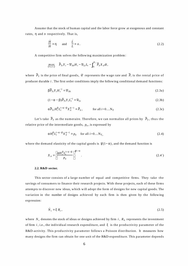
Assume that the stock of human capital and the labor force grow at exogenous and constant

rates, η and n respectively. That is,

˙ H

H= η and

˙ L

L= n . (2.2)

A competitive firm solves the following maximization problem:

maxH tLtXt

P YtYt − w HtH t − w LtLt − P itX itdi

0

N t∫ ,

where P Y is the price of final goods, w represents the wage rate and P i is the rental price of

producer durable i . The first order conditions imply the following conditional demand functions:

βP YtYtH t−1 = w Ht (2.3a)

(1 − α − β)P YtYtLt−1 = w Lt (2.3b)

αP YtHtβ Lt

1−α −β X itα −1 = P it , for all i=0....Nt (2.3c)

Let’s take P Y as the numeraire. Therefore, we can normalize all prices by P Y , thus the

relative price of the intermediate goods, pit , is expressed by

αHtβ Lt

1−α −β X itα −1 = pit for all i=0....Nt, (2.4)

where the demand elasticity of the capital goods is 1 (1− α) , and the demand function is

X it =αH t

β Lt1− α −β

pit

1 1 −α

. (2.4´)

2.2. R&D sector.

This sector consists of a large number of equal and competitive firms. They take the

savings of consumers to finance their research projects. With these projects, each of these firms

attempts to discover new ideas, which will adopt the form of designs for new capital goods. The

variation in the number of designs achieved by each firm is then given by the following

expression:

˙ N it = ξ Rit , (2.5)

where Nit denotes the stock of ideas or designs achieved by firm i , Rit represents the investment

of firm i , i.e., the individual research expenditure, and ξ is the productivity parameter of the

R&D-activity. This productivity parameter follows a Poisson distribution. It measures how

many designs the firm can obtain for one unit of the R&D-expenditure. This parameter depends

7

on the aggregate R&D-expenditure Rt and the aggregate stock of designs Nt . On the one hand,

the aggregate R&D-expenditure encourages the R&D effort, and so too the entry of firms in the

R&D sector. In this way, the aggregate R&D-expenditure increases the competition for

discovering new ideas, so that the number of designs obtained for each unit of expenditure

decreases. On the other hand, the stock of ideas increases the productivity of the R&D activity.

Hence, the productivity parameter ξ can be parameterized as

ξ = γRt

λ −1N t

φ , (2.6)

where λ and φ belong to (0,1) .

In the aggregate, the variation on the total number of designs is then given by the

following expression:

˙ N = γRt

λ Ntφ . (2.7)

From now on, we will assume that the R&D process exhibits constant returns to scale at the

aggregate level, i.e., λ + φ = 1.

Before closing this subsection, we must note that the stock of ideas or designs is now

determined by intentional R&D-expenditure made by the households. Consumers are owners of

the R&D firms. After having invested Rt units of income, they are the owners of the new design

that this investment produces. Thus, the return of this investment will be the flows that the

designs will yield. Each design is sold at a price PDt to an intermediate or capital-goods

producer. Therefore the free-entry condition can be stated as follows:

Rt (1− sR ) = PDt˙ N , (2.8)

where sR is the rate at which the government subsidizes investment in research.

2.3. Intermediate goods sector.

The intermediate sector is composed of an infinite number of firms on the interval 0, Nt[ ]that have purchased a design from the R&D sector. These firms transform a part of the

consumer’s savings into physical capital. This sector produces the durable goods that are

available to be used in final goods production at any time. Consider the simplest production

function:

X it = Sit , (2.9)

8

where Sit represents savings, which are rented at a rate rt , driven to the production of the

intermediate good i at time t . We are assuming that the capital is putty-putty, so that the firm

transforms units of durable goods back into general capital.

These goods X i are everlasting and do not depreciate. Firm i is the only seller of capital

good i , that is, each capital good producer is a local monopoly. Therefore, the monopoly price is

a simple markup over marginal cost, determined by the positive elasticity of demand 1 (1− α) ,

according to (2.4). This means:

pit = rt α . (2.10)

Government subsidizes the physical capital accumulation reducing the production cost of

these intermediate goods by sk . Note that a subsidy to physical capital accumulation might be

imposed directly on consumers as subsidy on investment or on producers as subsidy on investment

cost. Since the price pit is the same for all firms, and the output in equilibrium is also equal for

each different good, the net profits obtained for each monopolist are identical and given by:

Π it = pit Xit − rit Sit (1 − sk ) = Xt rt α − rt (1 − sk )( ) = rtX t

1− α(1 − sk)

α

= Πt . (2.11)

The decision to produce a new capital good also depends on a comparison between the price

that the firms must pay for the use of the design, PDt , and the discounted stream of net revenue.

Because the market for designs is competitive, their price will be bid down until it is equal to the

present value of the monopolist’s net profit. Therefore, at every moment in time the following

must hold:

PDt = e

− r sdst

τ∫ Πτ dτ

t

∞

∫ . (2.12)

Because of symmetry, each firm sets the same price and sells the same quantity of its

producer durable goods. Therefore we can express the total physical capital stock of economy Kt

by:

Kt = NtXt . (2.13)

2.4. Households.

We consider a representative household which has time-separable preferences with a

constant subjective rate of time preferences, ρ , and an instantaneous utility function

U(C) = C1−σ − 1( ) (1 − σ) , (2.14)

9

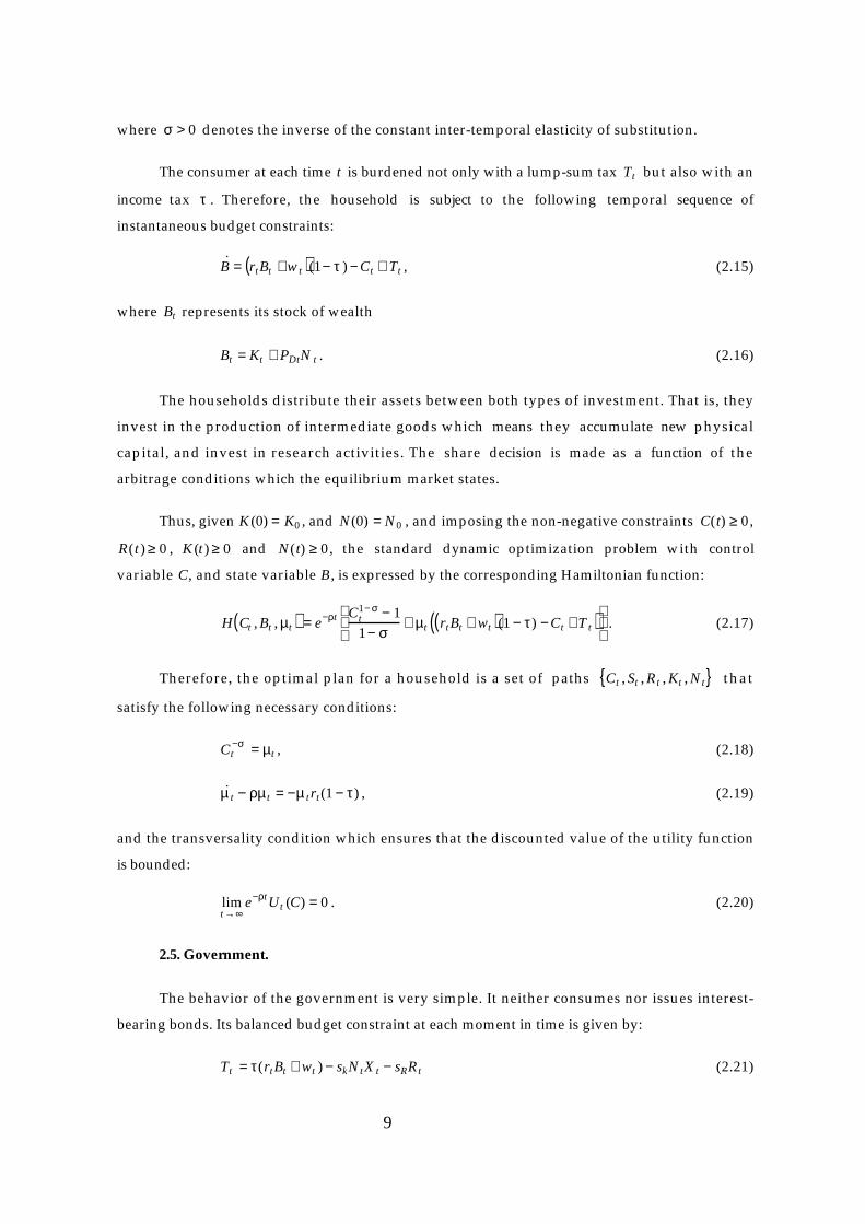
where σ > 0 denotes the inverse of the constant inter-temporal elasticity of substitution.

The consumer at each time t is burdened not only with a lump-sum tax Tt but also with an

income tax τ . Therefore, the household is subject to the following temporal sequence of

instantaneous budget constraints:

˙ B = rtBt + w t( )(1− τ ) − Ct + Tt , (2.15)

where Bt represents its stock of wealth

Bt = Kt + PDtN t . (2.16)

The households distribute their assets between both types of investment. That is, they

invest in the production of intermediate goods which means they accumulate new physical

capital, and invest in research activities. The share decision is made as a function of the

arbitrage conditions which the equilibrium market states.

Thus, given K (0) = K0 , and N(0) = N0 , and imposing the non-negative constraints C(t) ≥ 0,

R(t) ≥ 0 , K (t) ≥ 0 and N(t) ≥ 0, the standard dynamic optimization problem with control

variable C, and state variable B , is expressed by the corresponding Hamiltonian function:

H Ct , Bt , µt( ) = e −ρt Ct

1− σ − 1

1− σ+ µt rtBt + wt( )(1 − τ) − Ct + T t( )

. (2.17)

Therefore, the optimal plan for a household is a set of paths Ct , St , Rt , Kt , Nt that

satisfy the following necessary conditions:

Ct−σ = µt , (2.18)

˙ µ t − ρµ t = −µ trt(1 − τ) , (2.19)

and the transversality condition which ensures that the discounted value of the utility function

is bounded:

limt→∞

e −ρtUt (C) = 0 . (2.20)

2.5. Government.

The behavior of the government is very simple. It neither consumes nor issues interest-

bearing bonds. Its balanced budget constraint at each moment in time is given by:

Tt = τ(rtBt + wt ) − skNtX t − sRRt (2.21)

10

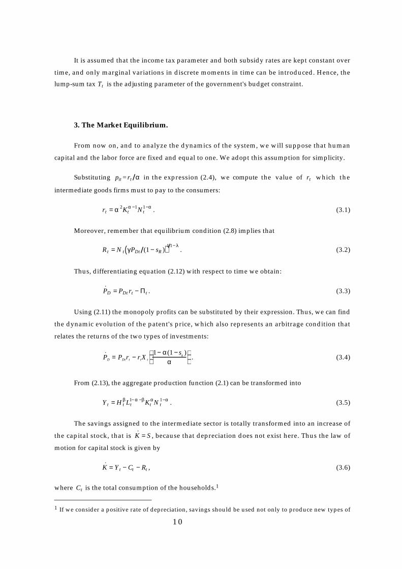
It is assumed that the income tax parameter and both subsidy rates are kept constant over

time, and only marginal variations in discrete moments in time can be introduced. Hence, the

lump-sum tax Tt is the adjusting parameter of the government's budget constraint.

3. The Market Equilibrium.

From now on, and to analyze the dynamics of the system, we will suppose that human

capital and the labor force are fixed and equal to one. We adopt this assumption for simplicity.

Substituting pit = rt α in the expression (2.4), we compute the value of rt which the

intermediate goods firms must to pay to the consumers:

rt = α 2Ktα −1Nt

1−α . (3.1)

Moreover, remember that equilibrium condition (2.8) implies that

Rt = N t γPDt (1 − sR )( )1 1− λ. (3.2)

Thus, differentiating equation (2.12) with respect to time we obtain:

˙ P D = PDt rt − Πt . (3.3)

Using (2.11) the monopoly profits can be substituted by their expression. Thus, we can find

the dynamic evolution of the patent's price, which also represents an arbitrage condition that

relates the returns of the two types of investments:

˙ P D = PDtrt − rtX t

1− α(1 − sk)

α

. (3.4)

From (2.13), the aggregate production function (2.1) can be transformed into

Yt = H tβ Lt

1− α −β KtαN t

1−α . (3.5)

The savings assigned to the intermediate sector is totally transformed into an increase of

the capital stock, that is ˙ K = S , because that depreciation does not exist here. Thus the law of

motion for capital stock is given by

˙ K = Yt − Ct − Rt , (3.6)

where Ct is the total consumption of the households.1

1 If we consider a positive rate of depreciation, savings should be used not only to produce new types of

11

Therefore according to equilibrium conditions (3.1) and (3.2), and the dynamical equations

(3.4) and (3.6), jointly with the first order condition (2.16), the dynamic system that defines the

equilibrium paths of the economy is composed of four differential equations that describe the

optimal behavior of the physical capital stock, the number of designs, the consumption and the

patent’s price, respectively. In other words, given the initial endowments of both designs and

physical capital, the market equilibrium of the economy is defined by the following system of

differential equations:

˙ K

K= Kt

α −1Nt1− α − Ct Kt − (Nt Kt ) γPDt (1 − sR )( )1 1 −λ

, (3.7a)

˙ N

N= γ γPDt (1− sR )( )1 1 − λ

, (3.7b)

˙ C

C=

1

σ(1 − τ )α 2Kt

α− 1Nt1−α − ρ( ) , (3.7c)

˙ P D

PD

= α 2Kt

α −1Nt

1−α − α 1− α(1 − sk )( )Kt

α Nt

−αPDt

−1 . (3.7d)

The dynamic system (3.17) reaches the steady state when N , K and C grow at a constant

rate, and PD is constant over time. Thus, to simplify the study of the transitional dynamics, we

transform the previous system (3.7) into one that presents a stationary equilibrium. Thus, we

consider the following two ratios: K N and C K , that will not grow in the steady state. In order

to check that, we first rewrite (3.7a) as follows:

ρ + σ

˙ C

C= α 2Kt

α −1Nt1−α . (3.8)

In the balanced growth path the consumption grows at a constant rate. Therefore, the expression

(3.8) only holds in the balanced growth path when the stock of capital and the number of designs

grow at the same rate.

On the other hand, from (3.2), (3.5), and using the previous conclusion, we can show that

R , Y and K also grow at the same rate in the balanced growth path. Thus, rewriting the

household’s budget constraint as Y K = ˙ K K + C K + R K , we can conclude that the ratio C K is

constant in the steady state.

Therefore, defining X = K N , Z = C K the dynamic behavior of the economy can also be

represented by the following reduced dynamic system in X , Z and PD

˙ X = Xα − ZX − γPD (1− sR )( )( 1 1 −λ )

− γ 1 1 −λ PD (1 − sR )( )(λ 1− λ )X , (3.9a)

capital goods, but also to replace the depreciation. However, the results of this paper would still remain valid.

12

˙ Z =

Z

σα 2X (α− 1) (1− τ ) − ρ( ) − ZX (α− 1) + Z2 + γ PD (1 − sR )( )1 1− λ

ZX −1 , (3.9b)

˙ P D = α 2X (α −1)PD − α 1− α(1 − sk)( )X α . (3.9c)

Since the initial value of X is totally defined by the initial stocks of physical capital

and the number of designs, given these initial stocks the dynamic system (3.9) and the

transversality condition (2.20) define the market equilibrium paths. They completely

characterize both the transitional dynamics and the steady-state equilibrium of the economy.

4. The Balanced Growth Path.

The long run equilibrium of this economy is given by Balance Growth Paths along which,

as we saw above, N , K , C , R , and Y grow at a constant and equal rate, and PD is constant over

time. In terms of the reduced system, this means that X , Z , PD stay constant over time.

Therefore, the steady state ( X , Z , P D ) can be computed by equating the growth rates of these

three variables to zero, from which the following system of equations is obtained:

X α −1 − Z − γP D (1 − sR )( )( 1 1 −λ )

X −1 − γ γP D (1 − sR )( )(λ 1− λ )= 0 , (4.1)

1

σα 2X (α −1) (1 − τ ) − ρ( ) − X (α −1) + Z + γP D (1− sR )( )( 1 1 − λ )

X −1 = 0 , (4.2)

α2X (α−1) − α 1− α (1− sk )( )X αP D

−1 = 0 . (4.3)

It is difficult to calculate the analytical solution of this system of equations. However, we

can still analyze the properties of it. The following result proves the existence and the

uniqueness of the steady-state equilibrium.

PROPOSITION 4.1. (i) If σ ≥ 1 , there always exists a unique balanced growth path. (ii)

When σ ∈(0,1) , a balanced growth path exists if the following condition holds:

ρσ(1 − σ )

1− α(1 − sk)

(1− α)

(1−α)

− γ 1 1−λ (1− α)

α (1− sR)

α 2 (1− σ)(1 − τ)

ρ

1 ( 1 −α)

(λ 1−λ )

−ρσ

> 0 .

Otherwise, no balanced growth path exists.

Proof: See Appendix A

13

Note that in this model there is endogenously determined sustainable growth, even if

there is no population growth.2 From (3.7b) we can affirm that the growth rate in the steady-

state equilibrium is given by the following expression:

g* = γ

γ P D(1 − sR )

1 1− λ

, (4.4)

which is directly obtained from equation (3.7b).

5. Stability of the Balanced Growth Path.

To examine the stability of the balanced equilibrium path, we set the fiscal parameters

equal to zero. Let us define x = ln(K N ), z = ln(C K ) and P = ln(PD) , then the dynamic behavior

of the economy can also be represented by the transformed dynamic system in x , z and P :

x = e (α− 1)x − e z − γ 1 1− λ e − x+ P( 1 1 − λ ) − γ 1 1 − λ e P (λ 1− λ ) ≡ Ψ(x , z, P) , (5.1a)

˙ z =

1

σα 2e(α −1) x − ρ( ) − e(α −1)x + e z + γ 1 1 −λ e− x+ P ( 1 1 −λ ) ≡ Ω(x , z, P), (5.1b)

˙ P = α 2e(α −1) x − α(1 − α )e αx− P ≡ Φ(x , z, P) . (5.1c)

Therefore, to study the local stability of the Balanced Growth Path, we will use the log-

linearization of the three dimensional dynamic system around the steady state equilibrium:

˙ x

˙ z

˙ P

=

Ψx Ψ z ΨP

Ω x Ωz Ω P

Φ x Φ z ΦP

x − x

z − z

P − P

. (5.2)

The elements of the coefficient matrix are the partial derivatives of ( x , ˙ z , ˙ P ) with respect

to x , z and P evaluated in the steady state. The sign of the eigenvalues of this matrix

determines the dynamics around the steady state. The following result characterizes the

convergence of the economy to its steady-state equilibrium.

2 In Jones' model sustainable growth only exists if the rate of population growth is positive. This model hasbeen dubbed the "semi-endogenous" growth model for this reason because economic policies do not affect thelong run growth rate.

14

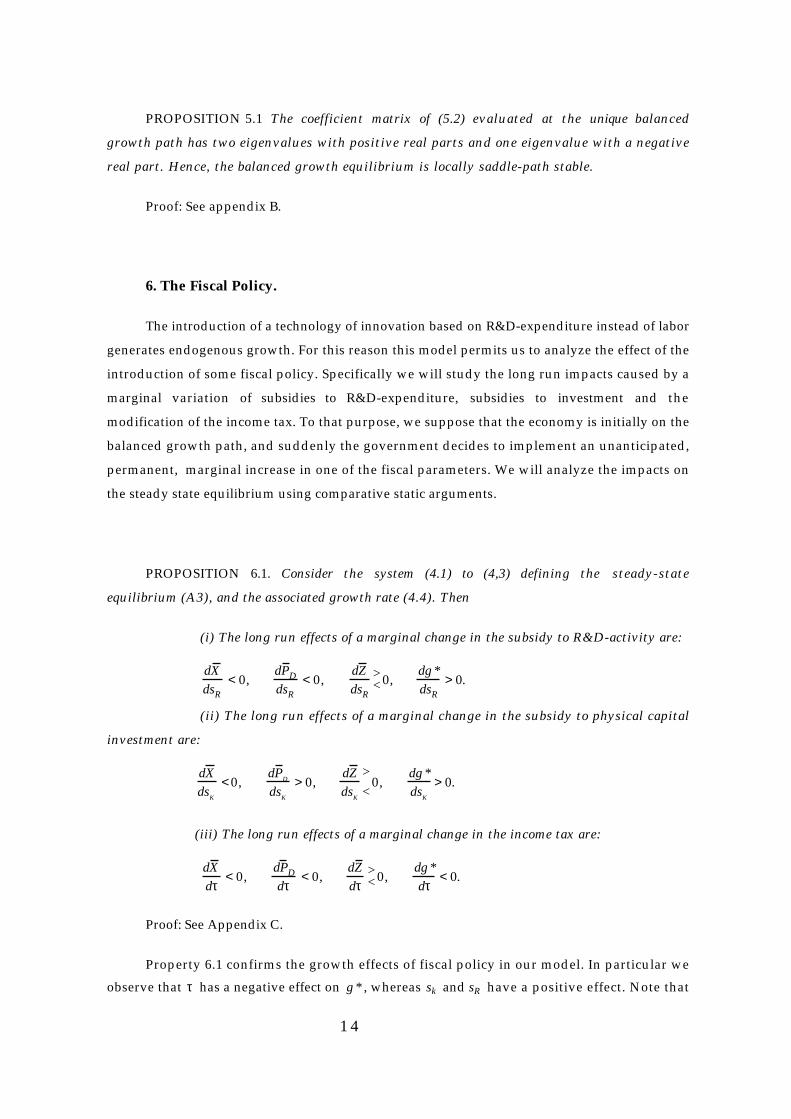
PROPOSITION 5.1 The coefficient matrix of (5.2) evaluated at the unique balanced

growth path has two eigenvalues with positive real parts and one eigenvalue with a negative

real part. Hence, the balanced growth equilibrium is locally saddle-path stable.

Proof: See appendix B.

6. The Fiscal Policy.

The introduction of a technology of innovation based on R&D-expenditure instead of labor

generates endogenous growth. For this reason this model permits us to analyze the effect of the

introduction of some fiscal policy. Specifically we will study the long run impacts caused by a

marginal variation of subsidies to R&D-expenditure, subsidies to investment and the

modification of the income tax. To that purpose, we suppose that the economy is initially on the

balanced growth path, and suddenly the government decides to implement an unanticipated,

permanent, marginal increase in one of the fiscal parameters. We will analyze the impacts on

the steady state equilibrium using comparative static arguments.

PROPOSITION 6.1. Consider the system (4.1) to (4,3) defining the steady-state

equilibrium (A3), and the associated growth rate (4.4). Then

(i) The long run effects of a marginal change in the subsidy to R&D-activity are:

dX

dsR

< 0, dP DdsR

< 0, dZ

dsR

><0,

dg *

dsR

> 0.

(ii) The long run effects of a marginal change in the subsidy to physical capital

investment are:

dX

dsK

< 0, dP

D

dsK

> 0, dZ

dsK

>

<0,

dg *

dsK

> 0.

(iii) The long run effects of a marginal change in the income tax are:

dX

dτ< 0,

dP Ddτ

< 0, dZ

dτ><0,

dg *

dτ< 0.

Proof: See Appendix C.

Property 6.1 confirms the growth effects of fiscal policy in our model. In particular we

observe that τ has a negative effect on g * , whereas sk and sR have a positive effect. Note that

15

the government can stimulate long run growth either directly through a subsidy to R&D-

expenditure, or indirectly by means of a subsidy to physical capital accumulation.

The growth effects of τ and sR are quite trivial, however it seems necessary to add some

comments about the effects of sk . The subsidy to physical capital accumulation reduces the

production cost of the intermediate capital goods. Hence, the net profits obtained by

monopolistic firms producing each good increase. This can induce two opposite, in some sense,

type of behaviors from intermediate firms. They can increase either the quantity produced of the

existing capital good or the demand of new designs. Since in this kind of models the intermediate

capital goods are complementary in the final production, increase the variety of these goods is

better for growth than increase the quantity produced of the existing ones. Therefore, the subsidy

to physical capital has positive effect on the demand of designs, which translates into an

increase in the patentee's price, and then, in a rise in the R&D effort. Observe that this subsidy

may also increase the production of the actual capital goods, however the result states that,

even in this case, the growth in the variety of capital goods is larger than the increase in

quantity produced of each capital good. Furthermore, we can show that there exists a

relationship between the growth effects of both subsidies, and these effects depend on the size of

those subsidies.

PROPOSITION 6.2. Let sR > 0 and sk > 0 . Consider a marginal change in both sR and sk .

Then,

dg *

dsR

≥<

dg *

dsk

if sR ≥

< 2α − 1

α− sk .

Proof: See Appendix C.

Notice that for the traditional estimated value α ≈ 0.36 , the inequality

sR > (2α − 1) α( ) − sk holds. This fact can easily be shown with the following corollary.

COROLLARY 6.3. There exists an α = 1 2 − sk( ) , such that for all values of α smaller than

α , dg * dsR > dg * dsk .

Finally, from the above results, the following states a negative impact that the taxes on

both types of investment have on economic growth.

16

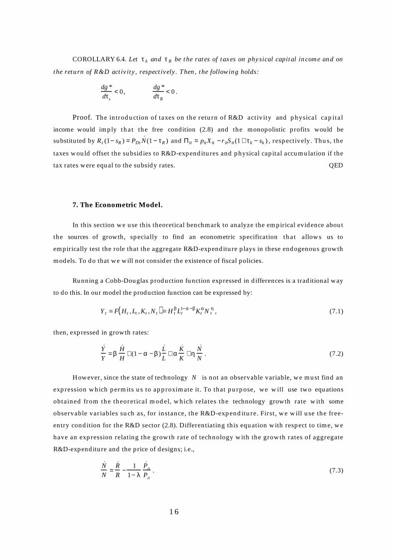
COROLLARY 6.4. Let τ k and τ R be the rates of taxes on physical capital income and on

the return of R&D activity, respectively. Then, the following holds:

dg *

dτk

< 0 , dg *

dτR

< 0 .

Proof. The introduction of taxes on the return of R&D activity and physical capital

income would imply that the free condition (2.8) and the monopolistic profits would be

substituted by Rt (1− sR ) = PDt˙ N (1 − τR ) and Πit = pitXit − r itSit(1 + τk − sk ) , respectively. Thus, the

taxes would offset the subsidies to R&D-expenditures and physical capital accumulation if the

tax rates were equal to the subsidy rates. QED

7. The Econometric Model.

In this section we use this theoretical benchmark to analyze the empirical evidence about

the sources of growth, specially to find an econometric specification that allows us to

empirically test the role that the aggregate R&D-expenditure plays in these endogenous growth

models. To do that we will not consider the existence of fiscal policies.

Running a Cobb-Douglas production function expressed in differences is a traditional way

to do this. In our model the production function can be expressed by:

Yt = F Ht , Lt , Kt , Nt( ) = H tβ Lt

1− α −β KtαN t

η , (7.1)

then, expressed in growth rates:

˙ Y

Y= β

˙ H

H+ (1 − α − β )

˙ L

L+ α

˙ K

K+ η

˙ N

N. (7.2)

However, since the state of technology N is not an observable variable, we must find an

expression which permits us to approximate it. To that purpose, we will use two equations

obtained from the theoretical model, which relates the technology growth rate with some

observable variables such as, for instance, the R&D-expenditure. First, we will use the free-

entry condition for the R&D sector (2.8). Differentiating this equation with respect to time, we

have an expression relating the growth rate of technology with the growth rates of aggregate

R&D-expenditure and the price of designs; i.e.,

˙ N

N=

˙ R

R−

1

1− λ

˙ P D

PD

. (7.3)

17

Hence, we will use this relationship to approximate the evolution of technology. From the

market equilibrium we observe that the growth rate of technology depends on how much firms

increase their expenditure on research and how the price of these new designs rises. Note that we

also introduce the role of the R&D-expenditure, which does not participate directly in the

production function. On the other hand, the growth rate of the patentee's price is one of the

equations of the dynamic system that describes the behavior of the economy. Thus, the second

step to obtain the approximation of the growth rate of technology (that we will estimate) is to

solve this system. In particular, we will use the policy function of the prices with respect to the

transformed variable x = ln(K N ).3 Then, after some calculations we can write the technology

growth rate as a linearly approximated function of the R&D-expenditure growth rate and a

dynamic factor. This last component depends on the distance between the initial level and the

steady state of the ratio from capital stock to the number of designs:

˙ N

N≈

˙ R

R−

1

1− λ(Φ x −Φ x )

1

eP

(x0 − x )exp(−θt) . (7.4)

In this expression θ denotes the absolute value of the stable eigenvalue of the dynamic

system (5.1), 1 e p( )′ is the associated eigenvector, and Φ x is an element of the Jacobian matrix

(5.2).4

Note that the second part of the right hand side is a number which depends on the time t .

Therefore we can approximate the growth rate of the technology, using a directly observable

component, which is controlled by economic agents, that is the R&D-expenditure growth rate

˙ R R , and a temporal component, ai exp(−θt) . Note that this temporal component includes a

constant factor, ai , which depends on the initial level and the steady state value of the ratio

capital stock-technology. Thus, if

− η

1

1− λ(Φx − Φx )

1

eP

(x0 − x )exp( −θt) = ai exp(−θt) ,

we can then transform (7.2) into

˙ Y

Y= β

˙ H

H+ (1 − α − β )

˙ L

L+ α

˙ K

K+ η

˙ R

R+ ai exp(−θt) . (7.5)

The fixed effect ai is different for each country, for this reason to estimate it we will

divide the total sample of countries into seven homogeneous subsamples, and then we will use one

dummy for each of them. These groups are the following, North America (USA and Canada),

3 This policy function tells us that the patentee's price level is determined by the distance between the initiallevel and the steady state of the ratio from capital stock to the number of designs.4 See Appendix D for a detailed explanation.

18

Oceania (New Zealand and Australia), Japan, the poorest EC countries (Greece, Portugal,

Ireland and Spain), the central EC countries (Belgium, Italy, Netherlands, France, Germany,

UK, Denmark and Austria) the Scandinavian EC countries (Finland and Sweden) and finally the

European non-EC countries (Norway and Switzerland). We include these seven dummies to

estimate ai because its value depends on the difference between the initial value and the steady

state of the ratio x on each country.

The following step is to try to analyze which elements determine this component

ai exp(−θt) . To that purpose, we use the same equations of the model used to derive equation

(7.5), but without considering the policy functions, i.e., we directly substitute in the dynamic

equation of prices as Appendix D shows. In this way, we approximate the growth rate of

technology by

˙ N

N=

˙ R

R−

α 2e(α −1)x

(1 − λ )(1 − λ )ln( R) + λ ln(N ) − ln(K) − ln γ + ln(α (1 − α ))[ ]. (7.6)

Finally, substituting (7.6) into (7.2), and using (3.5) to replace ln(N ) , we obtain

˙ Y

Y= β

˙ H

H+ (1 − α − β )

˙ L

L+ α

˙ K

K+ η

˙ R

R−

−

α 2e (α−1)x

(1− λ )λ ln(Y ) + λβ ln(H ) + λ (1− α − β )ln(L)(

+ η + αλ( )ln(K ) − η(1 − λ )ln( R) + (1 − α) ln γ − ln(α (1 − α ))( )) . (7.7)

Note that this equation is similar to (7.5) where the temporal component of the

technology, ai exp(−θt) , is determined by the initial levels of income, physical capital stock,

total human capital stock, the total labor, the R&D-expenditure, and the technology

parameters. We also include dummies for each group of countries as before because we must

estimate e(α −1) x which depends on the steady state of the ratio x of each country.

Next, we will present the results of the different estimations. We use the Non Linear

Squares Method.

8. The Empirical Results.

The model is estimated using pooled cross-section data for a sample of 21 OECD countries

with five observations for each country, which correspond to the differences for the years 1965,

1970, 1975, 1980, 1985 and 1990.

19

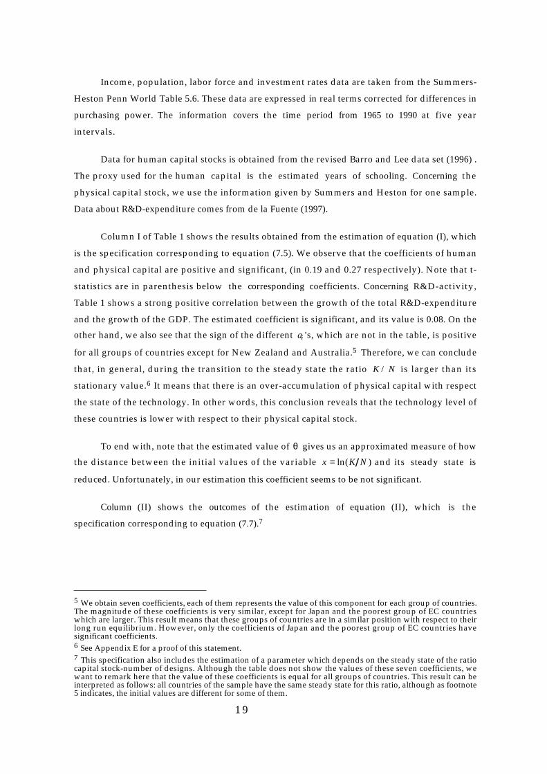
Income, population, labor force and investment rates data are taken from the Summers-

Heston Penn World Table 5.6. These data are expressed in real terms corrected for differences in

purchasing power. The information covers the time period from 1965 to 1990 at five year

intervals.

Data for human capital stocks is obtained from the revised Barro and Lee data set (1996) .

The proxy used for the human capital is the estimated years of schooling. Concerning the

physical capital stock, we use the information given by Summers and Heston for one sample.

Data about R&D-expenditure comes from de la Fuente (1997).

Column I of Table 1 shows the results obtained from the estimation of equation (I), which

is the specification corresponding to equation (7.5). We observe that the coefficients of human

and physical capital are positive and significant, (in 0.19 and 0.27 respectively). Note that t-

statistics are in parenthesis below the corresponding coefficients. Concerning R&D-activity,

Table 1 shows a strong positive correlation between the growth of the total R&D-expenditure

and the growth of the GDP. The estimated coefficient is significant, and its value is 0.08. On the

other hand, we also see that the sign of the different ai 's, which are not in the table, is positive

for all groups of countries except for New Zealand and Australia.5 Therefore, we can conclude

that, in general, during the transition to the steady state the ratio K / N is larger than its

stationary value.6 It means that there is an over-accumulation of physical capital with respect

the state of the technology. In other words, this conclusion reveals that the technology level of

these countries is lower with respect to their physical capital stock.

To end with, note that the estimated value of θ gives us an approximated measure of how

the distance between the initial values of the variable x = ln(K N ) and its steady state is

reduced. Unfortunately, in our estimation this coefficient seems to be not significant.

Column (II) shows the outcomes of the estimation of equation (II), which is the

specification corresponding to equation (7.7).7

5 We obtain seven coefficients, each of them represents the value of this component for each group of countries.The magnitude of these coefficients is very similar, except for Japan and the poorest group of EC countrieswhich are larger. This result means that these groups of countries are in a similar position with respect to theirlong run equilibrium. However, only the coefficients of Japan and the poorest group of EC countries havesignificant coefficients.6 See Appendix E for a proof of this statement.7 This specification also includes the estimation of a parameter which depends on the steady state of the ratiocapital stock-number of designs. Although the table does not show the values of these seven coefficients, wewant to remark here that the value of these coefficients is equal for all groups of countries. This result can beinterpreted as follows: all countries of the sample have the same steady state for this ratio, although as footnote5 indicates, the initial values are different for some of them.

20

Table 1. NLS Estimation Results.

(I) (II)

β 0.19(2.5)

β 0.05(1.3)

α 0.27(2.6)

α 0.22(3.1)

η 0.08(2.2)

η 0.08(2.6)

θ 0.36(1.1)

λ 0.94(1.1)

(I) ∆yit = β∆hit + (1 − α − β)∆lit + α∆k it + η∆rit + exp(−θt) a i∑ dum + ε t

(II) ∆yit = β∆hit + (1 − α − β)∆lit + α∆k it + η∆rit −

α 2 e (α −1)x i dum∑(1− λ )

λy t−5 + λβht−5 + λ (1 − α − β)lt−5(

+ η + αλ( )kt−5 − η(1 − λ )rt−5 + (1 − α) ln γ − ln(α (1 − α ))( )) + ε t .

With respect to this second estimation, we can see that the coefficient of human capital is

smaller than before and not significant. However, this result is not quite surprising. There are

recent empirical articles where the evidence on the relation between human capital and

economic growth is puzzling [see de la Fuente (1996), Freire-Serén (1999)]. Regarding the growth

rate of the aggregate R&D-expenditure, it has a significant and positive coefficient like in the

first estimation. Hence, we can conclude that the results about the coefficient of the aggregate

R&D-expenditure is robust to the specification. From this equation (7.7) we also estimate the

value of λ (and the outcome is 0.94). Note that λ represents the elasticity of the R&D-

expenditure with respect to the state of technology. Thus, a high value of λ means there is not

decreasing return on the R&D-expenditure. Therefore, the value of λ tells us that the R&D-

expenditure is very important for the generation of new technologies, and the evidence would

confirm that R&D-expenditure affects economic growth through its participation in the

production of new designs. However, this estimated coefficient is not significant.

21

9. Conclusion.

In this paper we have shown that the introduction of R&D-expenditure can generate

sustainable growth in the traditional R&D-based models of economic growth. Thus, the

continuous growth of the per capita income of countries can partially depend on the individuals'

choice of the amount of income devoted to finance the total cost of the R&D-activity. The

introduction of a technology of innovation based on R&D-expenditure instead of labor, generates

endogenous growth. For this reason this model has permitted us to analyze the growth effects of

some fiscal policies. More specifically, we have found that not only the introduction of a tax-

deduction to the R&D investment will encourage the innovation activity, but also the

introduction of a tax-deduction to the physical capital production. Thus, in the environment

defined for our model, the physical capital subsidy positively affects the long run growth rate

because it provides incentives to increase the variety of capital goods.

The paper also has empirically analyzed how R&D-expenditure affects productivity

growth. To that purpose, we have made use of an econometric model derived from the theoretical

one. More precisely, we have found an expression that can approximate the growth rate of

technology through the R&D-expenditure and other dynamical components. This expression has

been obtained using the free-entry condition that the competitive equilibrium states for the

R&D-activity and the policy function defining the dynamic evolution of patentees' price. At

this point, using cross-country data, we have found a positive and significant effect, and this

evidence seems to be quite robust. Then, the estimated coefficient corresponding to the R&D

regressor reveals a strong positive relationship between the growth of total R&D-expenditure

and the growth of the GDP. The estimated value of this coefficient tells us that a 1% rise in the

aggregate R&D-expenditure will increase the real GDP by 0.08%. Finally, we have tried to

estimate the value of the parameters defining the innovation technology. The results suggest

that the elasticity of the R&D-expenditure is close to one. Nevertheless, this estimated

coefficient does not appear significant.

APPENDICES

A. Proof of Proposition 4.1.

From (4.3) we derive the steady-state value X as a function of P D , i.e.,

X =

α1 − α(1 − s

k)( ) P D . (A1)

22

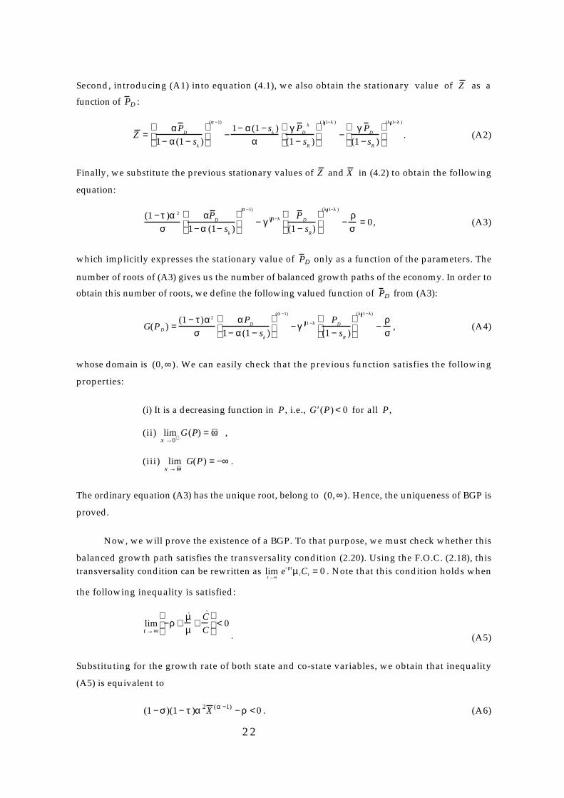
Second, introducing (A1) into equation (4.1), we also obtain the stationary value of Z as a

function of P D :

Z =

αP D

1− α(1 − sk)

(α −1)

−1− α(1 − s

k)

αγ P

D

λ

(1 − sR)

( 1 1−λ )

−γ P

D

(1 − sR)

(λ 1−λ )

. (A2)

Finally, we substitute the previous stationary values of Z and X in (4.2) to obtain the following

equation:

(1 − τ )α 2

σαP

D

1− α (1− sk)

(α −1)

− γ 1 1−λ P D

(1 − sR)

(λ 1−λ )

−ρσ

= 0, (A3)

which implicitly expresses the stationary value of P D only as a function of the parameters. The

number of roots of (A3) gives us the number of balanced growth paths of the economy. In order to

obtain this number of roots, we define the following valued function of P D from (A3):

G(PD ) =

(1 − τ)α2

σαP

D

1− α(1 − sk)

(α −1)

− γ 11 −λ PD

(1 − sR)

(λ 1−λ)

−ρσ

, (A4)

whose domain is (0, ∞). We can easily check that the previous function satisfies the following

properties:

(i) It is a decreasing function in P , i.e., G ′(P) < 0 for all P ,

(ii) lim

x →0+G(P) = +∞ ,

(iii) lim

x →+∞G(P) = −∞ .

The ordinary equation (A3) has the unique root, belong to (0, ∞). Hence, the uniqueness of BGP is

proved.

Now, we will prove the existence of a BGP. To that purpose, we must check whether this

balanced growth path satisfies the transversality condition (2.20). Using the F.O.C. (2.18), this

transversality condition can be rewritten as limt→∞

e−ρtµ tCt = 0 . Note that this condition holds when

the following inequality is satisfied:

limt→∞

−ρ +˙ µ µ

+˙ C

C

< 0

. (A5)

Substituting for the growth rate of both state and co-state variables, we obtain that inequality

(A5) is equivalent to

(1 − σ)(1 − τ )α 2X (α −1) − ρ < 0 . (A6)

23

When σ ≥ 1 inequality (A6) always holds, so that the transversality condition (2.18) is

satisfied. However, when σ ∈(0,1) , inequality (A6) holds if and only if

X > α 2 (1 − σ)(1 − τ) ρ( )1 ( 1 −α )

. (A7)

Using (A1) inequality (A7) can be expressed in terms of P D as follows:

P D >

(1 − α )

αα 2 (1 − σ)(1 − τ) ρ( )1(1−α)

. (A8)

Therefore, when σ ∈(0,1) the tranversality condition holds if the unique root of equation (A3)

satisfies inequality (A8). In other words, denote by A :

A =

(1 − α )

αα2 (1 − σ )(1 − τ ) ρ( )1 ( 1−α )

,

since G' (⋅) < 0 , and G(P D ) = 0, we know that G(A) > 0 . By substituting A for P D in (A4), we

obtain:

ρσ(1 − σ )

1− α(1 − sk)

(1− α)

(1−α)

− γ 1 1−λ (1− α)

α (1− sR)

α 2 (1− σ)(1 − τ)

ρ

1 ( 1 −α)

(λ 1−λ )

−ρσ

> 0 . (A9)

Hence when σ ∈(0,1) the root of equation (A3) defines a BGP if condition (A9) holds. Otherwise,

no BGP exists. The proposition is then proved. QED

B. Proof of Proposition 5.1.

We first calculate the coefficients of Jacobian matrix (5.2). Differentiating the dynamic

equations in system (5.1) with respect to x , z and P , and evaluating these derivatives at

x , z , P ( ) , we obtain

Ψx =

∂ ˙ x

∂x (x ,z , P )

= −(1 − α )e (α− 1)x + (γα (1 − α ))1 1− λ e x (λ 1−λ ) ,

Ψ z =

∂ ˙ x

∂z (x , z , P )

= −e z ,

ΨP =

∂ ˙ x

∂P (x ,z ,P )

= −(1 + λ )

(1 − λ )(γα (1 − α))1 1 −λ ex (λ 1− λ ) ,

Ωx =

∂ ˙ z

∂x (x , z ,P )

= −(1− α)

σα2e (α− 1)x + (1 − α)e(α −1)x − (γα (1 − α ))1 1− λ e x (λ 1− λ ) ,

24

Ω z =

∂ ˙ z

∂z (x , z ,P )

= ez ,

Ω P =

∂ ˙ z

∂P (x , z ,P )

=1

(1 − λ )(γα (1 − α))1 1 −λ ex (λ 1− λ ) ,

Φ x =∂ ˙ P

∂x(x , z , P )

= −α 2e(α −1)x ,

Φ z =∂ ˙ P

∂z(x , z ,P )

= 0 ,

Φ P =∂ ˙ P

∂P(x , z , P )

= α2 e(α− 1)x .

We now compute the three eigenvalues of Jacobian matrix (5.2), which are the solutions θ i

of the associated characteristic polynomial

−θ 3 + Aθ2 − Bθ + C = 0, (B1)

where A and C are respectively the trace and the determinant of Jacobian matrix (5.2), and

B = Ψx Ωz + Ψx ΦP + Ωz Φ P −Φ x ΨP − Ψ z Ωx . (B2)

In order to characterize the local stability of system (5.1), we must determine the sign of

the real parts of each θ i . To that purpose, we will use Routh's theorem.8 In this particular case,

the theorem says that the number of roots with positive real parts is equal to the number of

variations of sign in the following sequence: −1, A , −B + C A , C . Hence, to apply Routh's

theorem, we first consider the following results:

RESULT 1. The determinant of Jacobian matrix (5.2) is always negative.

Proof: From the Jacobian matrix we know that the determinant is given by

C = Ψx Ωz Φ P +Ψ z ΩP Φx − ΨP Ωz Φ x − Ψz Ω x ΦP . (B3)

Substituting for the derivatives computed at the beginning of this Appendix in (B3), we can

obtain

C = −

(1 − α)

σα2α 2e 2(α −1) x e z −

λ(1 − λ )

(γα (1 − α ))1 1− λ α 2e(α −1)x e z e x (λ 1−λ ) ,

8 See Grantmacher (1960) for more details.

25

which is negative. QED

RESULT 2. The trace of Jacobian matrix (5.2) is positive if σ > (1 − α ) .

Proof: From the Jacobian matrix we calculate the trace as follows:

A = Ψx + Ωz + ΦP . (B4)

Substituting for the derivatives computed at the beginning of this Appendix in (B4), we can

obtain

A = −(1 − α)e(α −1)x + (γα (1 − α ))1 1 −λ e x (λ 1− λ ) + e z + α 2e(α −1)x . (B5)

We know from (4.2) that the following relation holds:

−(1 − α )e (α− 1)x

= −

(1 − α)

σα 2e (α −1) x +

ρ(1 − α )

σ− (1 − α)ez − (1 − α)(γα (1− α))1 1 − λ e x (λ 1−λ ).

Therefore, introducing the previous equality in (B5), we can rewrite the trace as

A =

ρ(1 − α )

σ+ αe z + α(γα (1− α))1 1 − λ e x (λ 1−λ ) + α 2e (α −1) x σ − (1− α)

σ

,

which is positive when σ > (1 − α ) . QED

RESULT 3. B is negative if σ < (1 − α ) .

Proof: Substituting for the derivatives computed at the beginning of this Appendix in (B2),

we can rewrite B as follows:

B = −(1 − α)α 2e2( α −1)x

−α 2 (γα (1 − α ))1 1 −λ 2λ

(1 − λ )e x (λ 1−λ )e(α− 1)x − α2 e(α− 1)x ez (1 − α) − σ

σ

,

which is negative when σ < (1 − α ) . QED

Therefore, using the previous three results, we can prove Proposition 5.1. To this purpose,

we analyze the following two cases:

26

(i) σ > (1 − α ) . Since the trace and the determinant of Jacobian matrix (5.2) are

respectively positive and negative, two changes of sign in Routh's sequence always occur. Hence,

we have only one eigenvalue with a negative real part, so that the steady state is a saddle

point.

(ii) σ < (1 − α ) . In this case, the determinant of Jacobian matrix (5.2) and B are

both negative, whereas the trace can be either positive or negative. If the trace were positive,

we know from case (i) that the steady state is a saddle point. On the other hand, if the trace

were negative, the third element of Routh's sequence is positive, so that the same result holds.

C. Proof of Propositions 6.1 and 6.2.

First, applying the Implicit Function Theorem to equation (A3), we can calculate the impact of

the subsidies to investments in R&D and physical capital accumulation, and the income tax on

P D as follows

dP D

dsR

= −δG(P D ) δsR

δG(P D

) δP D

=λ γ

(1 − sR)

1 1−λ

P D

(λ 1−λ)

(1− λ )DP

< 0 , (C1)

dP D

dsk

= −δG(P D ) δsk

δG(P D) δP

=(α − 1)α 3 (1 − τ )

σ 1− α(1 − sk)( )DP

αP D

1− α(1 − sk)( )

(α −1)

> 0 , (C2)

dP D

dτ= −

δG(P D ) δτδG(P

D) δP

D

=α2 (1 − τ)(1 − s

k)1−α

σDP

α(1 − α )

P D

(α −1)

< 0 , (C3)

where

DP =δG(P

D)

δP D

=(α − 1)α2 (1 − τ)

σα

1− α(1 − sk)( )

(α −1)

P D(α −2)

−

λ1 − λ

γ 11 −λ (1− sR )−λ 1−λ P D( ) 2λ−11−λ( )

< 0 .

Using (A1) we can also compute the impact of the three fiscal policies on X as follows:

dX

dsR

=α

(1 − α)(1 − sk )

dP DdsR

< 0 , (C4)

dX

dsk

=α

1− α (1− sk)( )

dP D

dsk

−α 2

1− α(1 − sk)( )2 P D

27

=α 2λγ 1 1 −λ (1 − s

R)−λ 1−λ P

D

2λ−1 1− λ

1 − α(1 − sk)( )2

(1− λ )DP

< 0 , (C5)

dX

dτ=

α1− α (1− s

k)( )

dP D

dτ< 0. (C6)

With respect to the effect of the fiscal policies on Z , we differentiate (A2) with respect to

sR , sk and τ . However, one can easily check that the signs of the derivatives are ambiguous.

Finally, to analize the impact of the fiscal policies on the steady-state growth rate, we

differentiate (4.4) with respect to sR , sk and τ . Hence, using the previous results, we can prove

that

dg *

dsR

=γ

1− λγ P D

(1− sR )(λ − 2)

1 1 − λ

+γ

1− λγ P D

(2− λ )

(1 − sR )

1 1 −λdP DdsR

=α 2 (α − 1)(1− τ )

σ(1− λ )DP

γ(1 − s

R)

(2−λ ) ( 1−λ )

α1 − α(1 − s

k)( )

α −1

P D(α −2)+( 1 1−λ ) > 0, (C7)

dg *

dsk

=γ

1− λγ P

D

λ

(1− sR)

( 1 1−λ )

dP D

dsk

> 0, (C8)

dg *

dτ=

γ1− λ

γ P Dλ

(1− sR )

( 1 1− λ )dP Ddτ

< 0. (C9)

Before closing this section, we establish the relationship between the growth effects of sR

and sk . After some trivial algebra, we can write:

dg *

dsR

−dg *

dsk

=

γα 2(α − 1)(1 − τ)

σ(1− λ )DP

γ

(1 − sR)

1 1−λα

1− α(1 − sk)

α −1

P Dα −2+( 1 1−λ ) 1

(1 − sR)

−α

1− α (1− sk)( )

,

hence, the following can be checked:

Sing

dg *

dsR

−dg *

dsk

= Sing (1 − 2α ) + αsk + αsR[ ] . (C10)

D. The Econometric Model.

28

In this Appendix, we derive expressions (7.5) and (7.7) used in the econometric model. We

start with expression (7.4). From the main text we know that the production function is given by:

Yt = F Ht , Lt , Kt , Nt( ) = H tβ Lt

1− α −β KtαN t

η , (D1)

where N is an empirically unobservable variable. We will use relations (2.7) and (3.2) to obtain

an approximation for ˙ N N . In particular, to facilitate the explanation we consider the

following notation mt = Rt Nt . Thus, differentiating with respect to time (3.2) we obtain

˙ m

m=

1

1 − λ

˙ P DPD

=1

1− λ˙ P . (D2)

Introducing (5.1c) into (D2), we can rewrite:

˙ m

m=

1

1 − λα 2e(α −1)x − α(1 − α)eα x− P( ) ≡ G(x , P). (D3)

At this point, we make the first order Taylor approximation of (D3) around the steady

state, i.e.,

G(x , P) ≈ G(x , P ) + Gx GP ( ) x − x

P − P

, (D4)

where Gx GP ( ) is the Jacobian of G(x , P) evaluated in the steady state. We also note that

G(x , P ) is zero. Moreover, from (5.1c) we can write

G(x , P) =

1

1− λΦ(x , z, P), (D5)

where from Appendix B we know that Φ z is zero and Φ P = −Φx . Hence, we can rewrite (D4) as

follows

G(x , P) ≈

1

1− λΦx −Φ x ( ) x − x

P − P

. (D6)

We also know from the stability properties of Section 5 that the linear approximation of

the policy function of P is given by:

(P − P ) = (x0 − x )eP exp(−θt) , (D7)

where θ denotes the absolute value of the stable eigenvalue of Jacobian matrix (5.2), and

e P = Φx (−θ +Φx ) is the third component of the associated eigenvector. Thus, equation (D5)

transforms into

29

G(x , P) ≈

1

1− λΦx −Φ x ( ) (x0 − x )exp( −θt)

(x0 − x )e P exp(−θt)

. (D8)

Using (D3) and (D8), m m can be approximated by

˙ m

m≈

1

1 − λ(Φx −Φ x )

1

eP

(x0 − x )exp(−θt). (D9)

Moreover, since m m = ˙ R R − ˙ N N , we can state that

˙ N

N≈

˙ R

R−

1

1− λ(Φ x −Φ x )

1

eP

(x0 − x )exp(−θt) . (D10)

Therefore, expression (7.5) in the main text was obtained.

We now derive equation (7.7) used in the econometric model. From (5.2), and using

Appendix B, we can see that

˙ P = α 2e(α −1) x (P − x ) − (P − x )( ). (D11)

Furthermore, differentiating with respect to time (3.2), we also obtain

˙ P = (1 − λ )˙ R

R−

˙ N

N

. (D12)

Hence, introducing (D12), (3.2) and (A1) into (D11), and noting that x = ln(K ) − ln(N ) , we obtain

after simple algebra

˙ N

N=

˙ R

R−

α 2e(α −1)x

(1 − λ )(1 − λ )ln( R) + λ ln(N ) − ln(K) − ln γ + ln(α (1 − α ))[ ]. (D13)

Therefore, expression (7.6) in the main text was obtained.

E. The over-accumulation of physical capital during the transition.

In this Appendix, we show that the empirical result of a positive fixed effect implies

that there is an over-accumulation of physical capital with respect to the level of technology

during the transition to the steady-state equilibrium. In other words, we want to prove the if

ai > 0 then (x − x ) > 0 . First, we note from Appendix B that

˙ m

m≈

1

1 − λΦx −Φ x ( ) x − x

P − P

=

1

1 − λΦx (x − x ) − (P − P )( ). (E1)

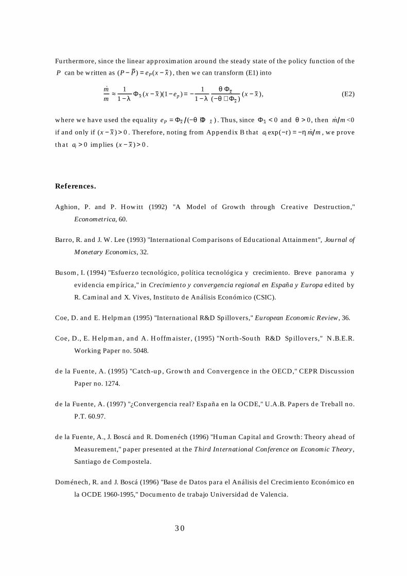
30

Furthermore, since the linear approximation around the steady state of the policy function of the

P can be written as (P − P ) = e P(x − x ) , then we can transform (E1) into

˙ m

m≈

1

1 − λΦ x (x − x )(1 − e p ) = −

1

1 − λθ Φx

(−θ + Φx )(x − x ), (E2)

where we have used the equality e P = Φx (−θ +Φx ) . Thus, since Φ x < 0 and θ > 0, then m m <0

if and only if (x − x ) > 0 . Therefore, noting from Appendix B that ai exp(−t) = −η ˙ m m , we prove

that ai > 0 implies (x − x ) > 0 .

References.

Aghion, P. and P. Howitt (1992) "A Model of Growth through Creative Destruction,"

Econometrica, 60.

Barro, R. and J. W. Lee (1993) "International Comparisons of Educational Attainment", Journal of

Monetary Economics, 32.

Busom, I. (1994) "Esfuerzo tecnológico, política tecnológica y crecimiento. Breve panorama y

evidencia empírica," in Crecimiento y convergencia regional en España y Europa edited by

R. Caminal and X. Vives, Instituto de Análisis Económico (CSIC).

Coe, D. and E. Helpman (1995) "International R&D Spillovers," European Economic Review, 36.

Coe, D., E. Helpman, and A. Hoffmaister, (1995) "North-South R&D Spillovers," N.B.E.R.

Working Paper no. 5048.

de la Fuente, A. (1995) "Catch-up, Growth and Convergence in the OECD," CEPR Discussion

Paper no. 1274.

de la Fuente, A. (1997) "¿Convergencia real? España en la OCDE," U.A.B. Papers de Treball no.

P.T. 60.97.

de la Fuente, A., J. Boscá and R. Domenéch (1996) "Human Capital and Growth: Theory ahead of

Measurement," paper presented at the Third International Conference on Economic Theory,

Santiago de Compostela.

Doménech, R. and J. Boscá (1996) "Base de Datos para el Análisis del Crecimiento Económico en

la OCDE 1960-1995," Documento de trabajo Universidad de Valencia.

31

Engelbrecht, H.-J (1997). "International R&D Spillovers, Human Capital and Productivity in

OECD Economies: An empirical Investigation" European Economic Review, 41.

Freire-Serén, M.J., (1999) "Human Capital Accumulation and Economic Growth," U.A.B.-I.A.E.

Working paper nº WP 435.99.

Gantmacher, F.R. (1960) "The Theory of Matrices," New York, Chelsea, vol II.

Grossman, G. and E. Helpman (1991a) "Innovation and Growth in the Global Economy," MIT

Press, Cambridge.

Grossman, G. and E. Helpman (1991b) "Quality Ladders in the Theory of Growth," Review of

Economic Studies, 58.

Grossman, G. and E. Helpman (1991c) "Quality Ladders and Product Cycles," Quarterly Journal of

Economics, 106.

Jones, C. (1991) "Empirical Evidence on R&D-Based Growth Models," Journal of Political

Economy , 58.

Jones, C. (1995) "Time Series Tests of Endogenous Growth Models," Quarterly Journal of

Economics, 110.

Lichtenberg, F. (1992) "R&D Investment and International Productivity Differences," NBER

Working Paper No. 4161.

Mankiw, G., D. Romer and D. Weil (1992) "A Contribution to the Empirics of Economic Growth,"

Quarterly Journal of Economics .

Romer, P. (1990) "Endogenous Technological Change," Journal of Political Economy, 98, no. 5.

Summers, R. and A. Heston, "The Penn World Table 5.6".