Embed Size (px)
Citation preview

© 2013 Pearson© 2013 Pearson

© 2013 Pearson
Aggregate Expenditure Multiplier
30CHECKPOINTS
Click on the button to go to the problem
© 2013 Pearson
Problem 1Problem 1
Problem 2Problem 2
Problem 1Problem 1
Problem 2Problem 2
In the newsIn the news
Checkpoint 30.1 Checkpoint 30.3
Problem 1Problem 1
Checkpoint 30.2
Clickerversion
Clickerversion
Clickerversion
Clickerversion
Clickerversion
Clickerversion
Problem 3Problem 3
Problem 2Problem 2
Problem 3Problem 3
Problem 4Problem 4
Problem 3Problem 3Clickerversion
Clickerversion
Clickerversion
ClickerversionIn the newsIn the news
In the newsIn the news

Click on the button to go to the problem
© 2013 Pearson
Problem 2Problem 2
Problem 1Problem 1
Checkpoint 30.4
In the newsIn the news

© 2013 Pearson
Practice Problem 1 The marginal propensity to consume is 0.8.
If disposable income increases by $0.5 trillion, by how much will consumption expenditure change?
CHECKPOINT 30.1
© 2013 Pearson
SolutionThe marginal propensity to consume is the fraction of a change in disposable income that is spent on consumption.
Consumption expenditure will increase by 0.8 multiplied by the change in disposable income of $0.5 trillion.
Consumption expenditure will increase $0.4 trillion.
CHECKPOINT 30.1
© 2013 Pearson
Practice Problem 2 Explain how each of the following events influences the U.S. consumption function:
• The marginal propensity to consume decreases.
• U.S. autonomous consumption decreases.
• Americans expect an increase in future income.
CHECKPOINT 30.1
© 2013 Pearson
SolutionThe marginal propensity to consume equals the slope of the consumption function.
So when the marginal propensity to consume decreases, the consumption function becomes flatter.
Autonomous consumption is the y-axis intercept of the consumption function.
So when autonomous expenditure decreases, the consumption function shifts downward.
CHECKPOINT 30.1
© 2013 Pearson
When expected future income increases, current consumption expenditure increases.
The consumption function shifts upward.
CHECKPOINT 30.1
© 2013 Pearson
Study Plan ProblemWhen the marginal propensity to consume decreases, the U.S. consumption function ___________.
CHECKPOINT 30.1
A. becomes flatter
B. becomes steeper
C. shifts upward
D. shifts downward
© 2013 Pearson
When when autonomous expenditure decreases, the U.S. consumption function ___________.
CHECKPOINT 30.1
A. becomes flatter
B. becomes steeper
C. shifts upward
D. shifts downward
© 2013 Pearson
When expected future income increases, the U.S. consumption function ___________.
CHECKPOINT 30.1
A. becomes flatter
B. becomes steeper
C. shifts upward
D. shifts downward
© 2013 Pearson
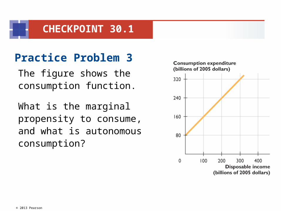
Practice Problem 3 The figure shows the consumption function.
What is the marginal propensity to consume, and what is autonomous consumption?
CHECKPOINT 30.1
© 2013 Pearson
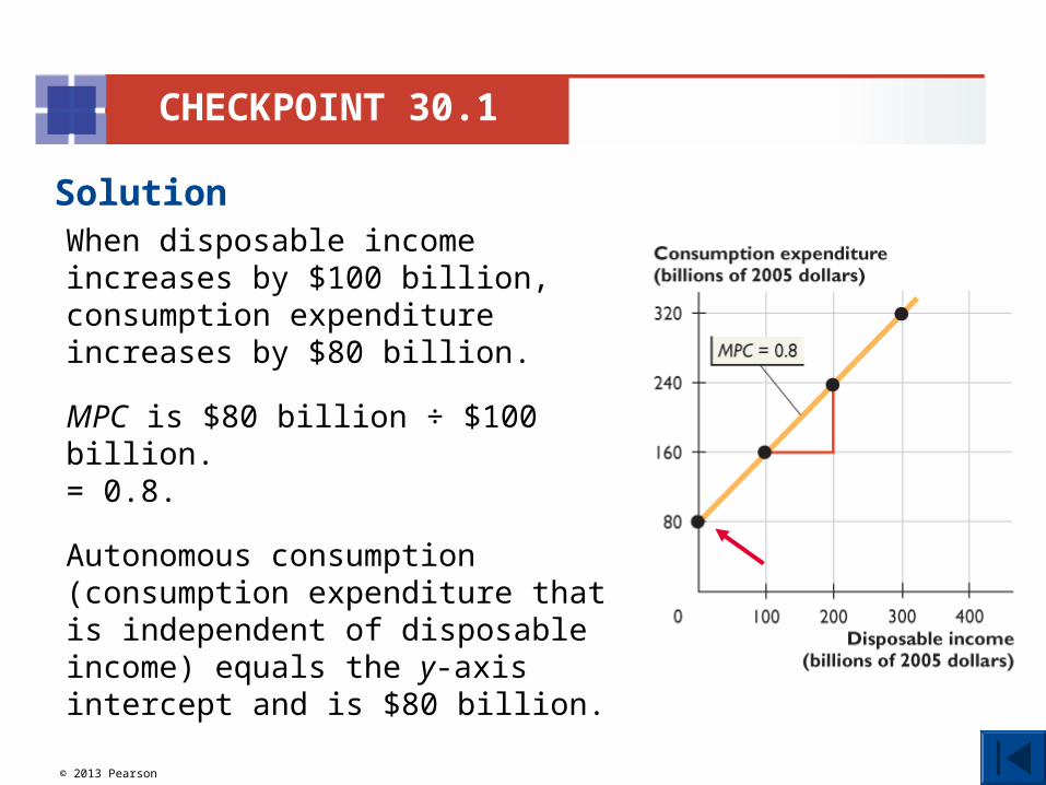
SolutionWhen disposable income increases by $100 billion, consumption expenditure increases by $80 billion.
MPC is $80 billion ÷ $100 billion. = 0.8.
Autonomous consumption (consumption expenditure that is independent of disposable income) equals the y-axis intercept and is $80 billion.
CHECKPOINT 30.1
© 2013 Pearson
In the newsPersonal income falls as spending rises
Personal income fell 0.1% in August, after increasing 0.1% in July, while personal spending rose just 0.2% in August, after rising 0.8% in July.
Source: CNN Money, September 30, 2011
How can consumers increase spending when personal income falls?
Does the rise in consumer spending arise from a movement along the consumption function or a shift of the consumption function? Explain your answer.
CHECKPOINT 30.1
© 2013 Pearson
SolutionOther things remaining the same, a fall in personal income brings a fall in consumption expenditure in a movement along the consumption function.
When an incraese in consumption expenditure occurs at the same time that personal income decreases, the consumption function has shifted upward.
Autonomous consumption expenditure has increased as households spent part of their past savings.
CHECKPOINT 30.1
© 2013 Pearson
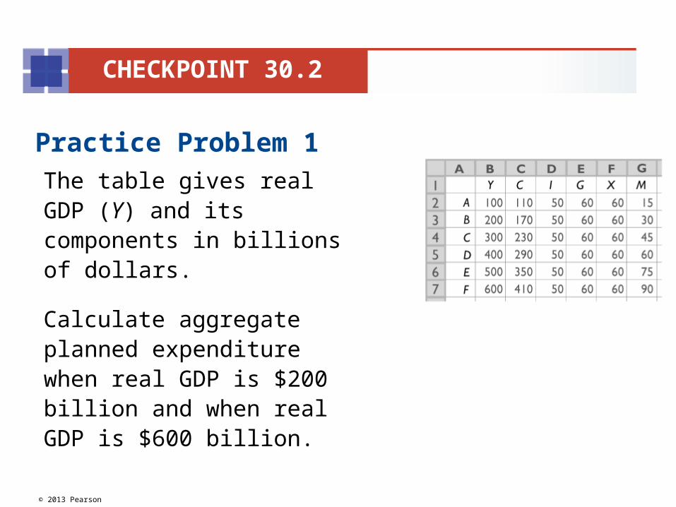
Practice Problem 1 The table gives real GDP (Y) and its components in billions of dollars.
Calculate aggregate planned expenditure when real GDP is $200 billion and when real GDP is $600 billion.
CHECKPOINT 30.2
© 2013 Pearson
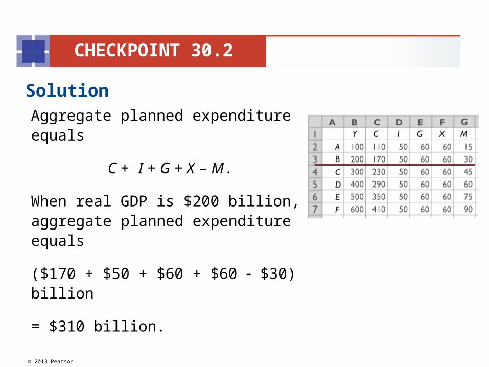
SolutionAggregate planned expenditure equals
C + I + G + X – M.
When real GDP is $200 billion, aggregate planned expenditure equals
($170 + $50 + $60 + $60 $30) billion
= $310 billion.
CHECKPOINT 30.2
© 2013 Pearson
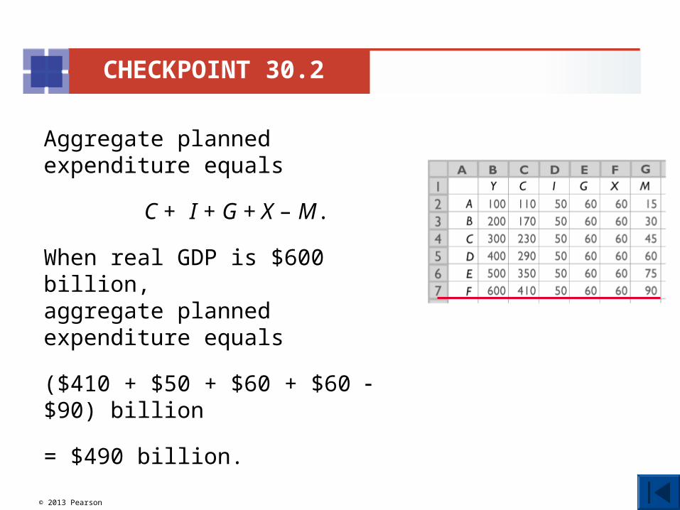
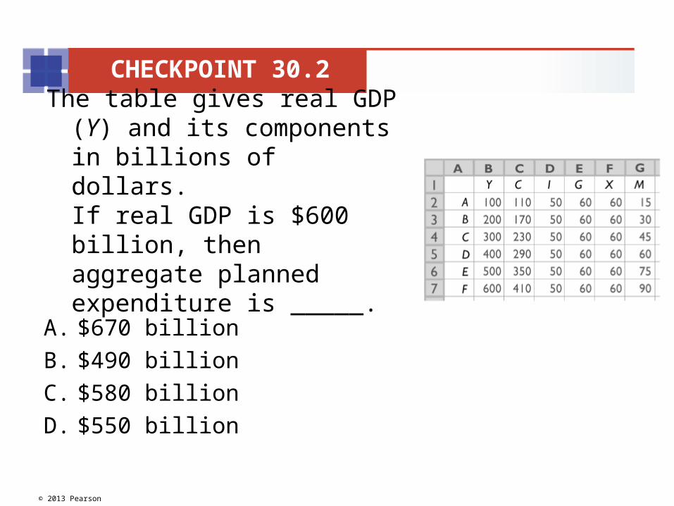
Aggregate planned expenditure equals
C + I + G + X – M.
When real GDP is $600 billion, aggregate planned expenditure equals
($410 + $50 + $60 + $60 $90) billion
= $490 billion.
CHECKPOINT 30.2
© 2013 Pearson
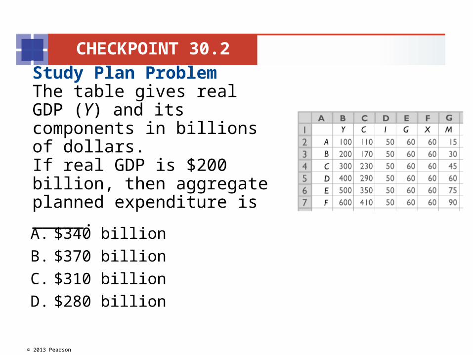
Study Plan Problem The table gives real GDP (Y) and its components in billions of dollars.If real GDP is $200 billion, then aggregate planned expenditure is _____.
CHECKPOINT 30.2
A. $340 billion
B. $370 billion
C. $310 billion
D. $280 billion
© 2013 Pearson
The table gives real GDP (Y) and its components in billions of dollars.If real GDP is $600 billion, then aggregate planned expenditure is _____.
CHECKPOINT 30.2
A. $670 billion
B. $490 billion
C. $580 billion
D. $550 billion
© 2013 Pearson
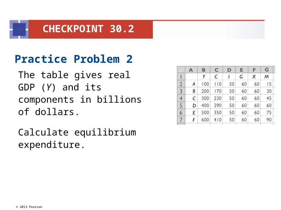
Practice Problem 2 The table gives real GDP (Y) and its components in billions of dollars.
Calculate equilibrium expenditure.
CHECKPOINT 30.2
© 2013 Pearson
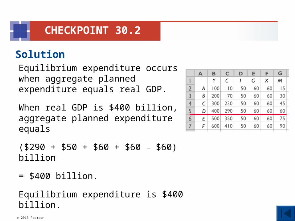
SolutionEquilibrium expenditure occurs when aggregate planned expenditure equals real GDP.
When real GDP is $400 billion, aggregate planned expenditure equals
($290 + $50 + $60 + $60 – $60) billion
= $400 billion.
Equilibrium expenditure is $400 billion.
CHECKPOINT 30.2
© 2013 Pearson
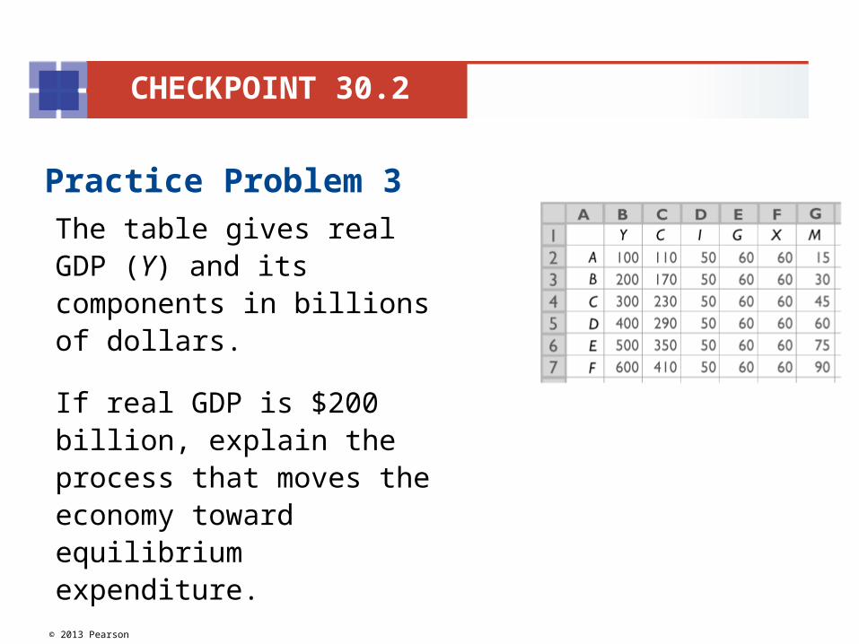
Practice Problem 3 The table gives real GDP (Y) and its components in billions of dollars.
If real GDP is $200 billion, explain the process that moves the economy toward equilibrium expenditure.
CHECKPOINT 30.2
© 2013 Pearson
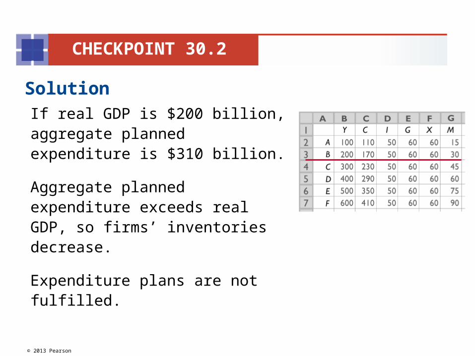
SolutionIf real GDP is $200 billion, aggregate planned expenditure is $310 billion.
Aggregate planned expenditure exceeds real GDP, so firms’ inventories decrease.
Expenditure plans are not fulfilled.
CHECKPOINT 30.2
© 2013 Pearson
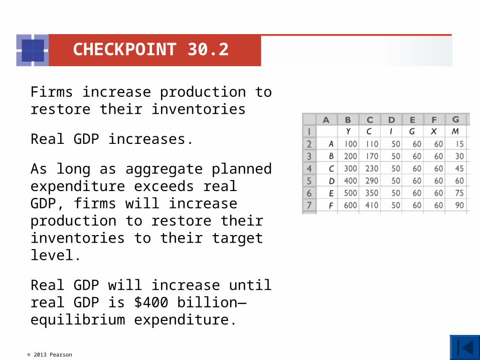
Firms increase production to restore their inventories
Real GDP increases.
As long as aggregate planned expenditure exceeds real GDP, firms will increase production to restore their inventories to their target level.
Real GDP will increase until real GDP is $400 billion—equilibrium expenditure.
CHECKPOINT 30.2
© 2013 Pearson
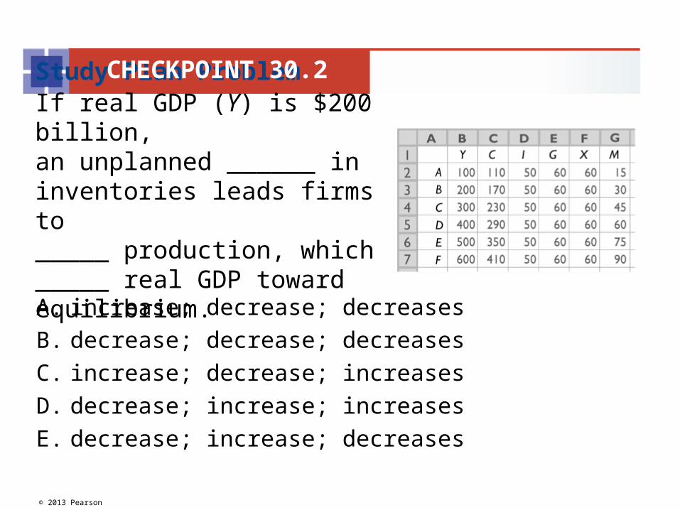
Study Plan Problem If real GDP (Y) is $200 billion, an unplanned ______ in inventories leads firms to_____ production, which _____ real GDP toward equilibrium.
CHECKPOINT 30.2
A. increase; decrease; decreases
B. decrease; decrease; decreases
C. increase; decrease; increases
D. decrease; increase; increases
E. decrease; increase; decreases

© 2013 Pearson
Practice Problem 4 The table gives real GDP (Y) and its components in billions of dollars.
If real GDP is $600 billion, explain the process that moves the economy toward equilibrium expenditure.
CHECKPOINT 30.2
© 2013 Pearson
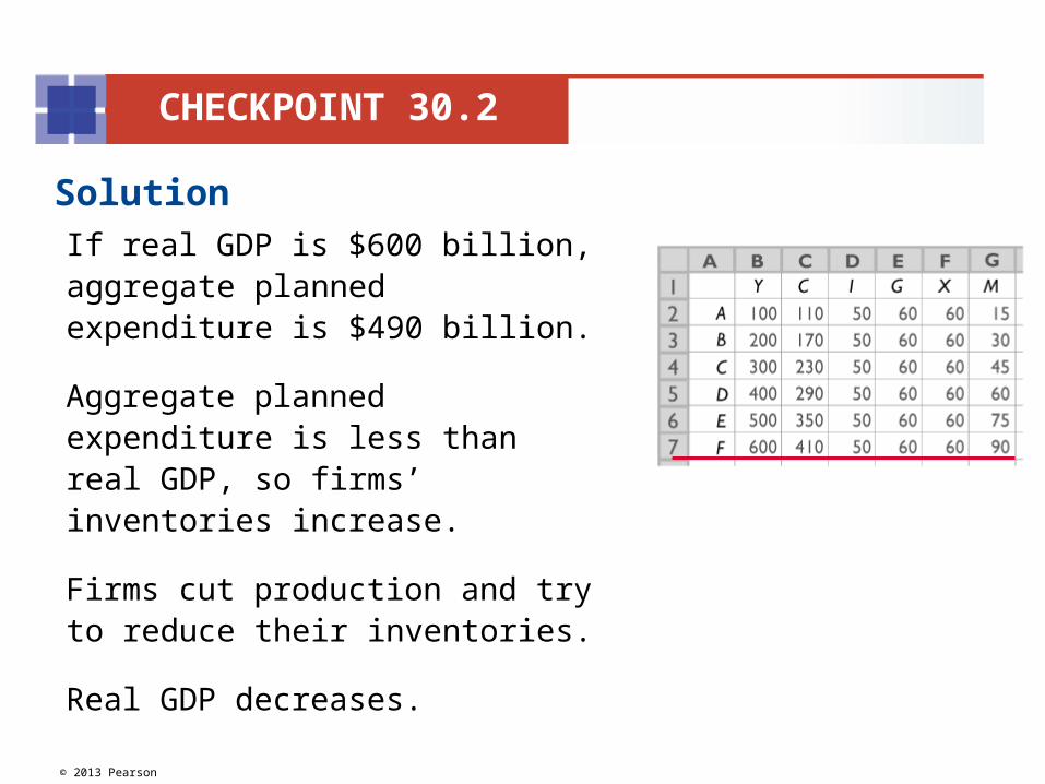
SolutionIf real GDP is $600 billion, aggregate planned expenditure is $490 billion.
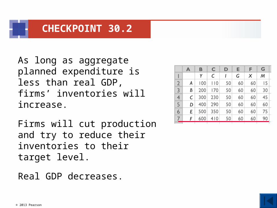
Aggregate planned expenditure is less than real GDP, so firms’ inventories increase.
Firms cut production and try to reduce their inventories.
Real GDP decreases.
CHECKPOINT 30.2
© 2013 Pearson
As long as aggregate planned expenditure is less than real GDP, firms’ inventories will increase.
Firms will cut production and try to reduce their inventories to their target level.
Real GDP decreases.
CHECKPOINT 30.2
© 2013 Pearson
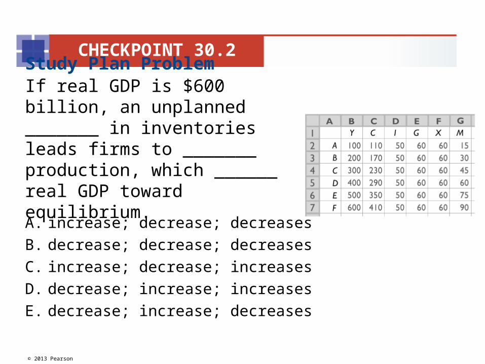
Study Plan Problem If real GDP is $600 billion, an unplanned _______ in inventories leads firms to _______ production, which ______ real GDP toward equilibrium.
CHECKPOINT 30.2
A. increase; decrease; decreases
B. decrease; decrease; decreases
C. increase; decrease; increases
D. decrease; increase; increases
E. decrease; increase; decreases
© 2013 Pearson
In the newsWholesale inventories decline, sales rise
Wholesale inventories fell 1.3 percent in August, which helped depress economic output during the recession. Rising sales might encourage businesses to begin restocking their inventories, which would help boost economic growth.
Source: The New York Times, October 8, 2009
Explain why a fall in inventories is associated with recession and a restocking of inventories might bolster economic growth.
CHECKPOINT 30.2
© 2013 Pearson
SolutionWhen firms reduce their target level of inventories, planned investment falls and equilibrium expenditure and real GDP decrease—as occurred during the year to August 2009.
When firms plan to restock their inventories, the reverse occurs. Equilibrium expenditure and real GDP increase.
CHECKPOINT 30.2
© 2013 Pearson
Practice Problem 1An economy has no imports and no income taxes, MPC is 0.80, and real GDP is $150 billion.
Businesses increase investment by $5 billion.
Calculate the multiplier and the change in real GDP.
CHECKPOINT 30.3
© 2013 Pearson
SolutionThe multiplier equals 1/(1 – MPC).
MPC is 0.8, so the multiplier is 5.
The multiplier = Change in real GDP ÷ Investment
Change in real GDP = Investment × Multiplier
= $5 billion × 5.
Real GDP increases by $25 billion.
The increase in investment increases real GDP by the multiplier (5) times the change in investment ($5 billion).
CHECKPOINT 30.3
© 2013 Pearson
Practice Problem 2An economy has no imports and no income taxes, MPC is 0.80, and real GDP is $150 billion.
Businesses increase investment by $5 billion.
Calculate the new level of real GDP and explain why real GDP increases by more than $5 billion.
CHECKPOINT 30.3
© 2013 Pearson
SolutionThe multiplier equals 1/(1 – MPC).
MPC is 0.8, so the multiplier is 5.
The increase in investment increases real GDP by the multiplier (5) times the change in investment ($5 billion).
Real GDP increases by $25 billion to $175 billion.
Real GDP increases by more than $5 billion because the increase in investment induces an increase in consumption expenditure.
CHECKPOINT 30.3
© 2013 Pearson
Practice Problem 3An economy has no imports and no income taxes.
An increase in autonomous expenditure of $2 trillion increases equilibrium expenditure by $8 trillion.
Calculate the multiplier and the marginal propensity to consume.
CHECKPOINT 30.3
© 2013 Pearson
SolutionThe multiplier equals the increase in equilibrium expenditure ($8 trillion) divided by the increase in autonomous expenditure ($2 trillion).
The multiplier is 4.
The multiplier is 1/(1 – MPC).
So 4 = 1/(1 – MPC), and MPC is 0.75.
The marginal propensity to consume is 0.75.
CHECKPOINT 30.3
© 2013 Pearson
Study Plan Problem In an economy has no imports and no income taxes, an increase in autonomous expenditure of $2 trillion increases equilibrium expenditure by $8 trillion.Calculate the multiplier and the marginal propensity to consume.
CHECKPOINT 30.3
A. 4; 0.25
B. 0.25; –3.0
C. 4; 0.75
D. 0.75; 4

© 2013 Pearson
In the newsKeystone XL pipeline—Alberta to the Gulf of Mexico
TransCanada says building the $7 billion pipeline would put 20,000 Americans directly to work during the construction phase and add an expected 118,000 spin-off jobs. The project would also pump $20 billion into the U.S. economy.
Source: CNN Money, September 30, 2011
Explain how TransCanada’s investment of $7 billion could create spin-off jobs and pump $20 billion into the U.S. economy.
CHECKPOINT 30.3
© 2013 Pearson
SolutionThe investment of $7 billion will increase real GDP by more than $7 billion because the investment multiplier exceeds 1.
When construction begins, new jobs are created and these workers will receive an income.
They will spend part of it on consumption goods and services, which in turn will create jobs in other industries—spin-off jobs.
CHECKPOINT 30.3

© 2013 Pearson
These workers will earn an income.
They will spend part of the income on consumption goods and services.
TransCanada says that the multiplier is $20 billion ÷ $7 billion, which is almost 3, an optimistic estimate.
CHECKPOINT 30.3
© 2013 Pearson
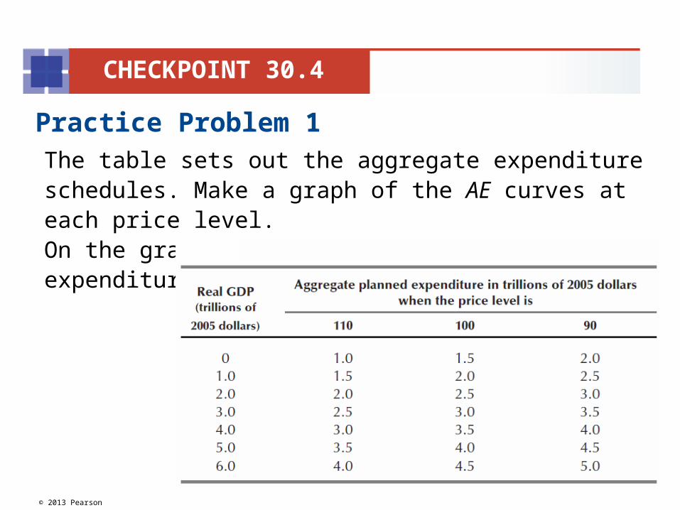
Practice Problem 1The table sets out the aggregate expenditure schedules. Make a graph of the AE curves at each price level.On the graph, mark the equilibrium expenditure at each price level.
CHECKPOINT 30.4
© 2013 Pearson
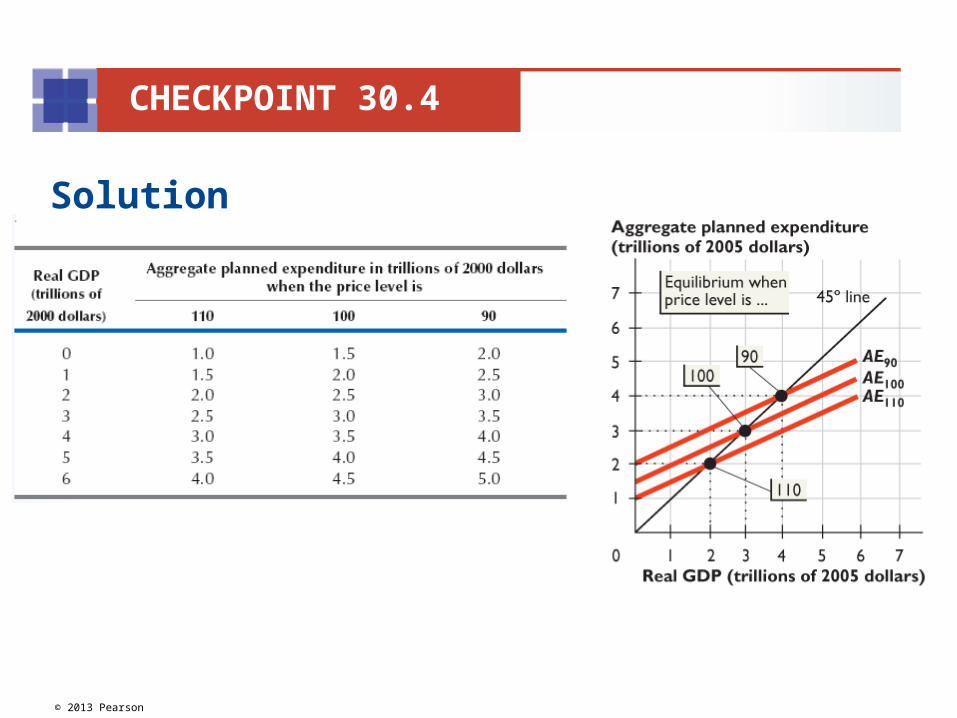
Solution
CHECKPOINT 30.4
© 2013 Pearson
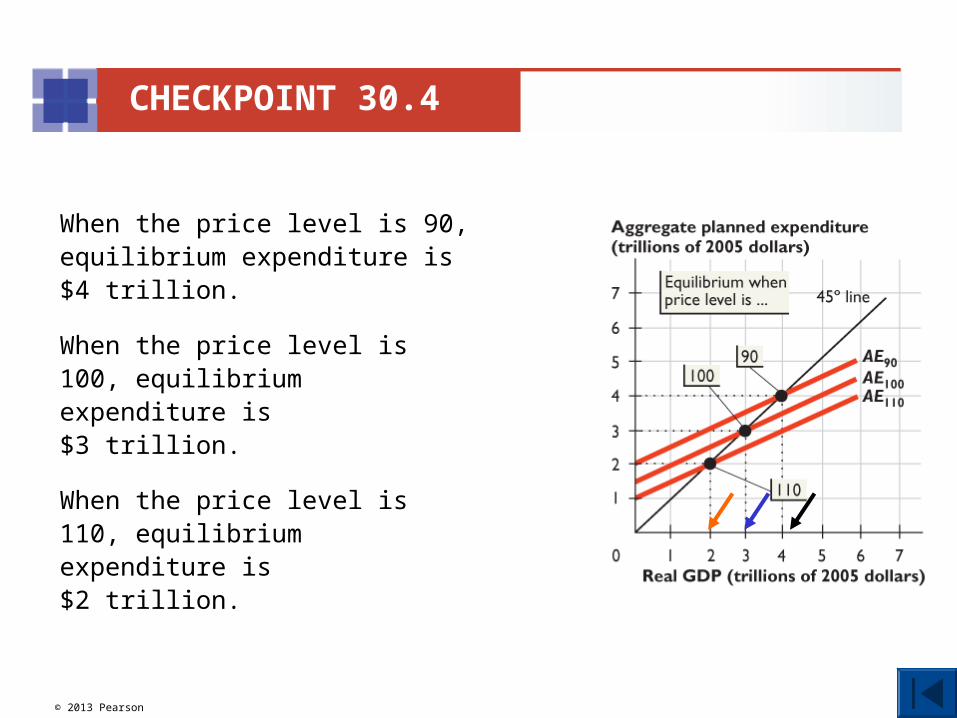
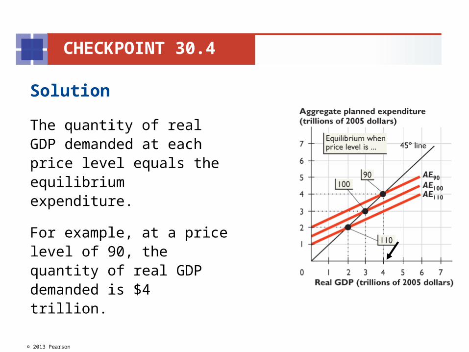
When the price level is 90, equilibrium expenditure is $4 trillion.
When the price level is 100, equilibrium expenditure is $3 trillion.
When the price level is 110, equilibrium expenditure is $2 trillion.
CHECKPOINT 30.4
© 2013 Pearson
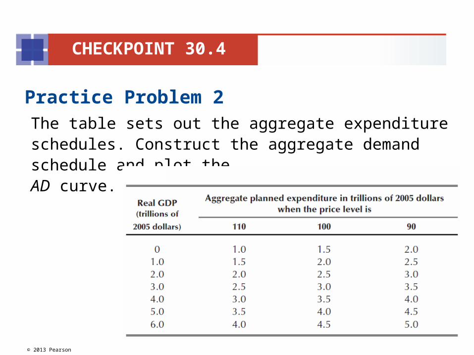
Practice Problem 2The table sets out the aggregate expenditure schedules. Construct the aggregate demand schedule and plot the AD curve.
CHECKPOINT 30.4
© 2013 Pearson
Solution
The quantity of real GDP demanded at each price level equals the equilibrium expenditure.
For example, at a price level of 90, the quantity of real GDP demanded is $4 trillion.
CHECKPOINT 30.4
© 2013 Pearson
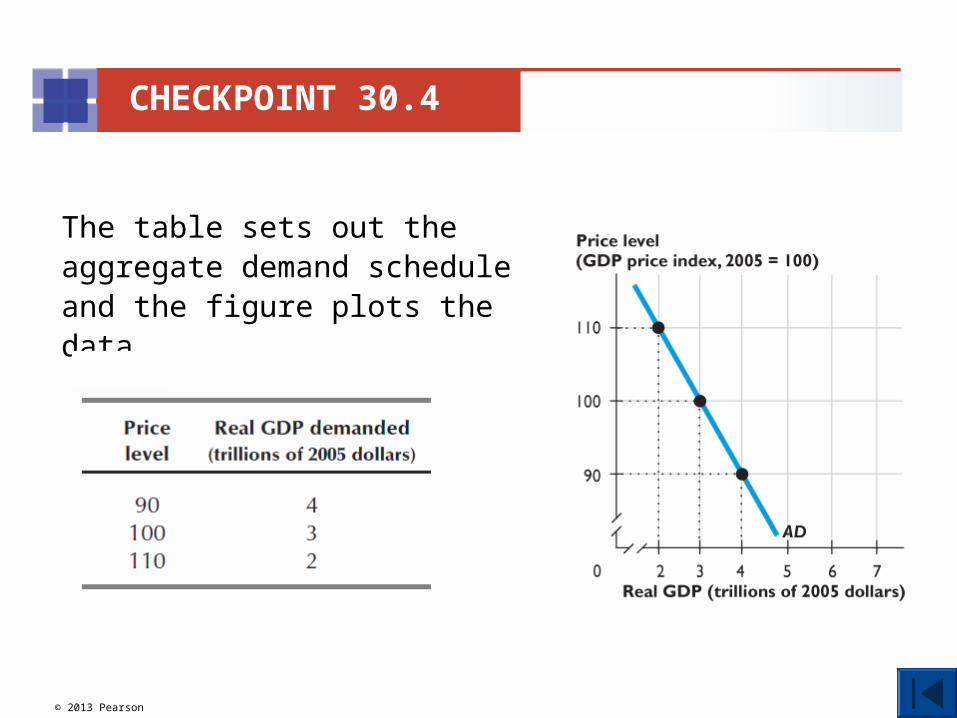
The table sets out the aggregate demand schedule and the figure plots the data.
CHECKPOINT 30.4
© 2013 Pearson
In the newsPrice jump worst in 3 yearsAn increase in the price of essentials such as oil, food and cotton left U.S. consumers struggling with the highest inflation rate in three years.
Source: CNN Money, September 26, 2011
Explain the effect of a rise in the price level on equilibrium expenditure.
CHECKPOINT 30.4

© 2013 Pearson
Solution
A rise in the price level decreases consumption expenditure, which decreases aggregate planned expenditure and shifts the AE curve downward.
Equilibrium expenditure decreases.
CHECKPOINT 30.4