Embed Size (px)
DESCRIPTION
Lecture (7): Matlab Graphics - Sulaimani University - College of Science - Physics Department
Citation preview
1
Matlab Graphics
Introduction to Matlab 7
Omed Ghareb AbdullahSulaimani UniversitySulaimani UniversityCollege of SciencesCollege of SciencesPhysics DepartmentPhysics Department
1
3D graphIn this section we will focus on the basic MATLAB i t ti f l tti 3 D h MATLAB instructions for plotting a 3-D graph and controlling its appearance.Ref: help graph3d
2
2
meshgrid• meshgrid generates x and y grid coordinates of a
rectangular mesh.g• Example:
x=linspace(-5,5,30);
y=linspace(-2,2,20);
[X,Y]=meshgrid(x,y);
ill d t 5 b 6 t i i d iwill produce two 5 by 6 matrices xi and yiwhich contain the x and y coords, respectively, of a 5 by 6
rectangular grid. xi and yi can now be used as templates when interpolating randomly
scattered data into a uniform grid for contour and surface plotting routines as shown by the next slide.
3
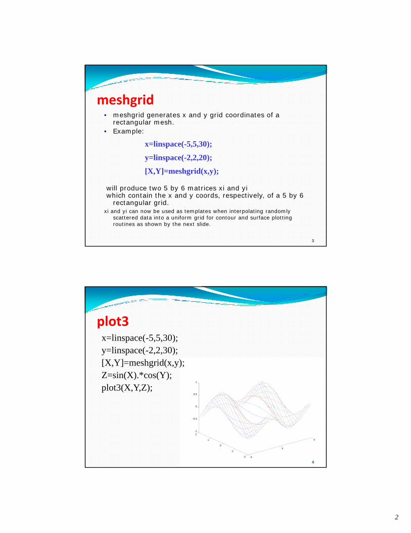
plot3x=linspace(-5,5,30);
li ( )
0
0.5
1
y=linspace(-2,2,30);[X,Y]=meshgrid(x,y);Z=sin(X).*cos(Y);plot3(X,Y,Z);
-5
0
5
-2
-1
0
1
2-1
-0.5
4
3
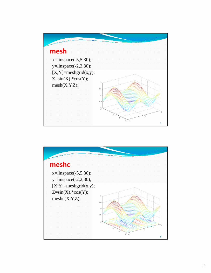
meshx=linspace(-5,5,30);
li ( )y=linspace(-2,2,30);[X,Y]=meshgrid(x,y);Z=sin(X).*cos(Y);mesh(X,Y,Z);
5
meshcx=linspace(-5,5,30);
li ( )y=linspace(-2,2,30);[X,Y]=meshgrid(x,y);Z=sin(X).*cos(Y);meshc(X,Y,Z);
6
4
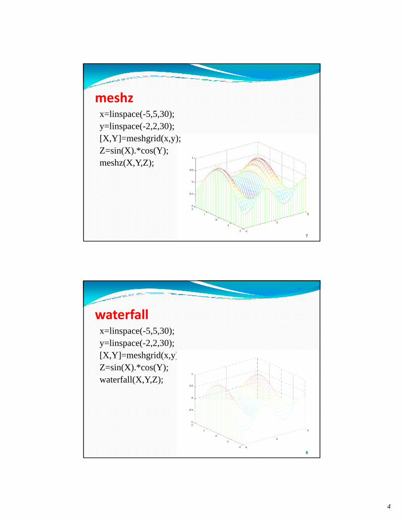
meshzx=linspace(-5,5,30);
li ( )y=linspace(-2,2,30);[X,Y]=meshgrid(x,y);Z=sin(X).*cos(Y);meshz(X,Y,Z);
7
waterfallx=linspace(-5,5,30);
li ( )y=linspace(-2,2,30);[X,Y]=meshgrid(x,y);Z=sin(X).*cos(Y);waterfall(X,Y,Z);
0
0.5
1
-5
0
5
-2
-1
0
1
2-1
-0.5
8
5
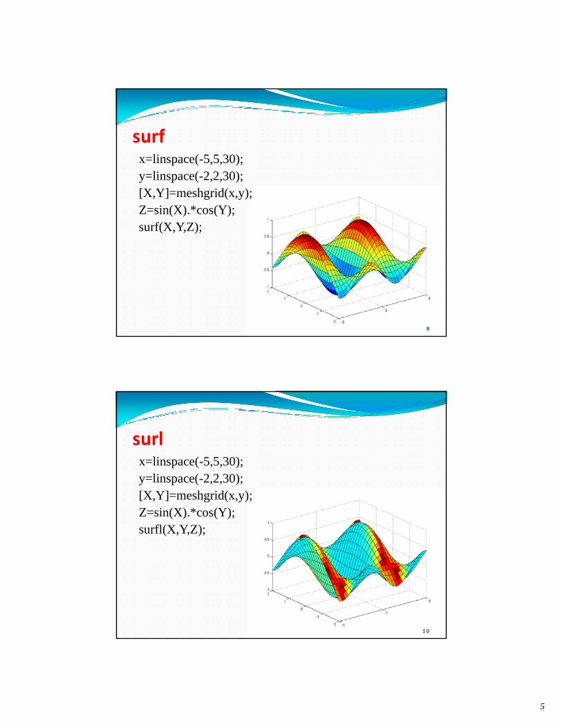
surfx=linspace(-5,5,30);
li ( )y=linspace(-2,2,30);[X,Y]=meshgrid(x,y);Z=sin(X).*cos(Y);surf(X,Y,Z);
9
surlx=linspace(-5,5,30);
li ( )y=linspace(-2,2,30);[X,Y]=meshgrid(x,y);Z=sin(X).*cos(Y);surfl(X,Y,Z);
10
6
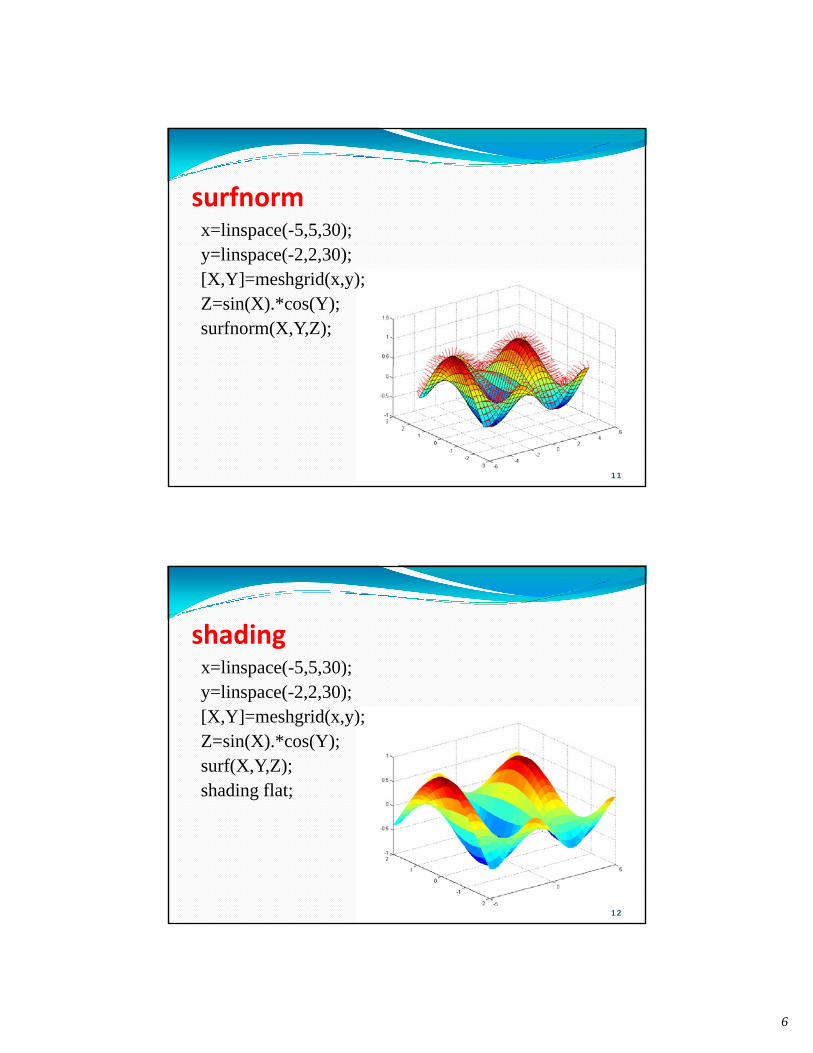
surfnormx=linspace(-5,5,30);
li ( )y=linspace(-2,2,30);[X,Y]=meshgrid(x,y);Z=sin(X).*cos(Y);surfnorm(X,Y,Z);
11
shadingx=linspace(-5,5,30);
li ( )y=linspace(-2,2,30);[X,Y]=meshgrid(x,y);Z=sin(X).*cos(Y);surf(X,Y,Z);shading flat;
12
7
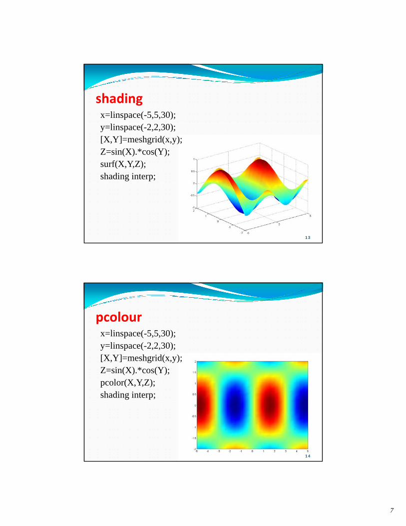
shadingx=linspace(-5,5,30);
li ( )y=linspace(-2,2,30);[X,Y]=meshgrid(x,y);Z=sin(X).*cos(Y);surf(X,Y,Z);shading interp;
13
pcolourx=linspace(-5,5,30);
li ( )y=linspace(-2,2,30);[X,Y]=meshgrid(x,y);Z=sin(X).*cos(Y);pcolor(X,Y,Z);shading interp;
14
8
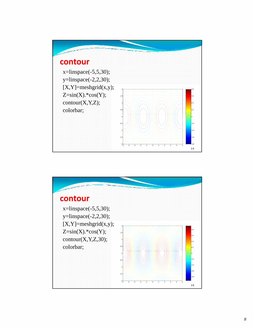
contourx=linspace(-5,5,30);
li ( )
0.5
1
1.5
2
0.2
0.4
0.6
0.8
y=linspace(-2,2,30);[X,Y]=meshgrid(x,y);Z=sin(X).*cos(Y);contour(X,Y,Z); colorbar;
-5 -4 -3 -2 -1 0 1 2 3 4 5-2
-1.5
-1
-0.5
0
-0.8
-0.6
-0.4
-0.2
0
15
contourx=linspace(-5,5,30);
li ( )
0.5
1
1.5
2
0.2
0.4
0.6
0.8
y=linspace(-2,2,30);[X,Y]=meshgrid(x,y);Z=sin(X).*cos(Y);contour(X,Y,Z,30); colorbar;
-5 -4 -3 -2 -1 0 1 2 3 4 5-2
-1.5
-1
-0.5
0
-0.8
-0.6
-0.4
-0.2
0
16
9
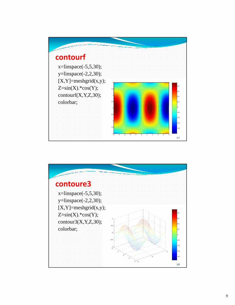
contourfx=linspace(-5,5,30);
li ( )
0.5
1
1.5
2
0.2
0.4
0.6
0.8
y=linspace(-2,2,30);[X,Y]=meshgrid(x,y);Z=sin(X).*cos(Y);contourf(X,Y,Z,30); colorbar;
-5 -4 -3 -2 -1 0 1 2 3 4 5-2
-1.5
-1
-0.5
0
-0.8
-0.6
-0.4
-0.2
0
17
contoure3x=linspace(-5,5,30);
li ( )
0
0.5
1
0.2
0.4
0.6
0.8
y=linspace(-2,2,30);[X,Y]=meshgrid(x,y);Z=sin(X).*cos(Y);contour3(X,Y,Z,30);colorbar;
-5
0
5
-2
-1
0
1
2-1
-0.5
-0.8
-0.6
-0.4
-0.2
0
18
10
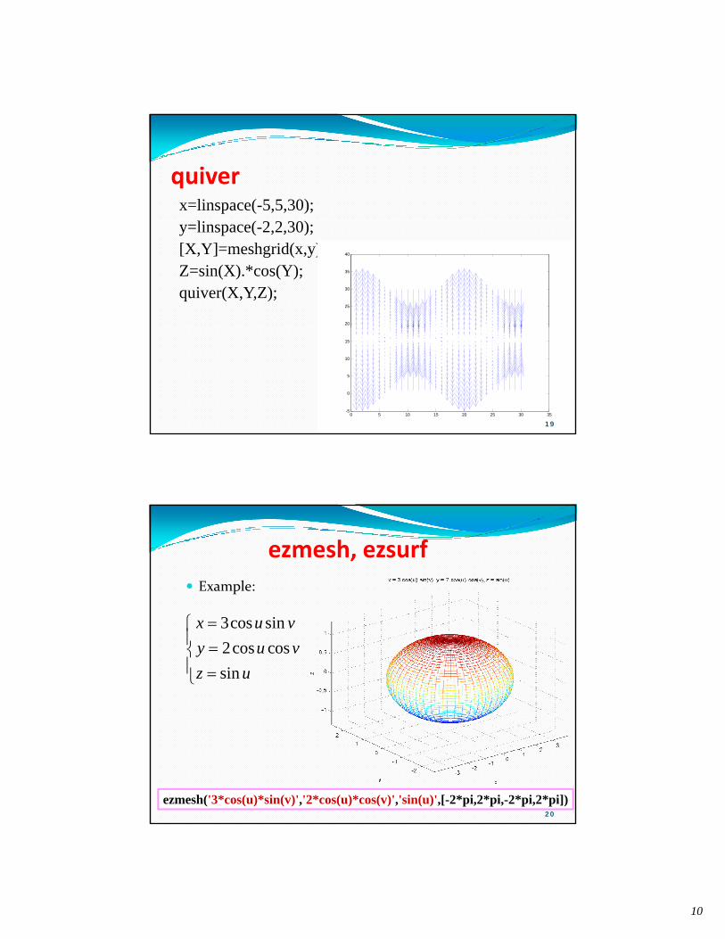
quiverx=linspace(-5,5,30);
li ( )y=linspace(-2,2,30);[X,Y]=meshgrid(x,y);Z=sin(X).*cos(Y);quiver(X,Y,Z);
20
25
30
35
40
0 5 10 15 20 25 30 35-5
0
5
10
15
19
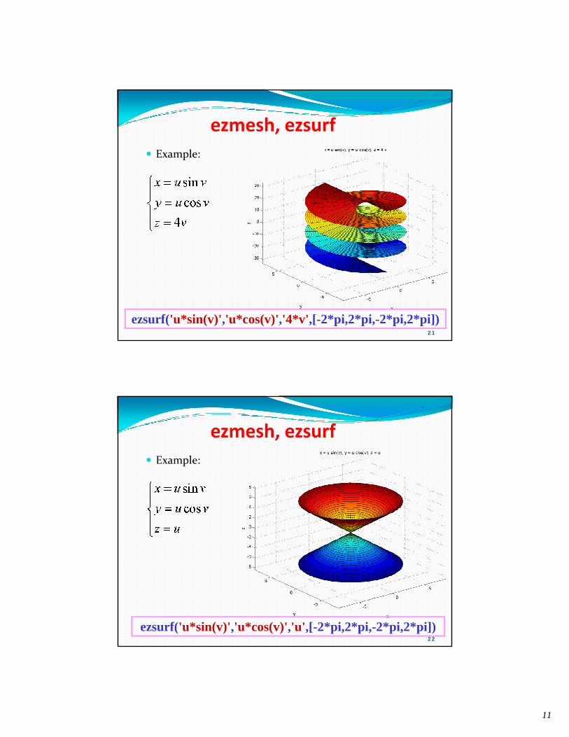
ezmesh, ezsurfExample:
3cos sin2cos cossin
x u vy u vz u
=⎧⎪ =⎨⎪ =⎩
ezmesh('3*cos(u)*sin(v)','2*cos(u)*cos(v)','sin(u)',[-2*pi,2*pi,-2*pi,2*pi])20
11
Example:
ezmesh, ezsurf
ezsurf('u*sin(v)','u*cos(v)','4*v',[-2*pi,2*pi,-2*pi,2*pi])21
Example:
ezmesh, ezsurf
ezsurf('u*sin(v)','u*cos(v)','u',[-2*pi,2*pi,-2*pi,2*pi])22
12
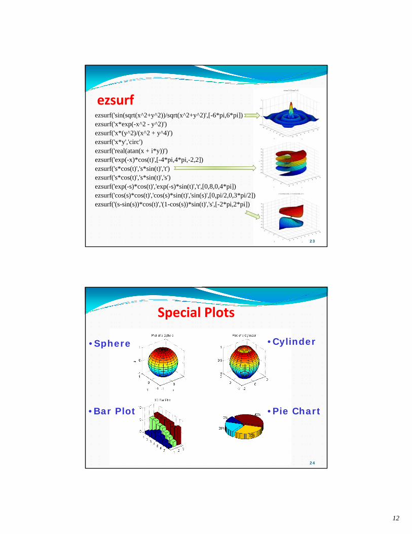
ezsurfezsurf('sin(sqrt(x^2+y^2))/sqrt(x^2+y^2)',[-6*pi,6*pi])ezsurf('x*exp(-x^2 - y^2)')ezsurf( x exp( x 2 y 2) )ezsurf('x*(y^2)/(x^2 + y^4)')ezsurf('x*y','circ')ezsurf('real(atan(x + i*y))')ezsurf('exp(-x)*cos(t)',[-4*pi,4*pi,-2,2])ezsurf('s*cos(t)','s*sin(t)','t')ezsurf('s*cos(t)','s*sin(t)','s')ezsurf('exp( s)*cos(t)' 'exp( s)*sin(t)' 't' [0 8 0 4*pi])ezsurf( exp(-s)*cos(t) , exp(-s)*sin(t) , t ,[0,8,0,4*pi])ezsurf('cos(s)*cos(t)','cos(s)*sin(t)','sin(s)',[0,pi/2,0,3*pi/2])ezsurf('(s-sin(s))*cos(t)','(1-cos(s))*sin(t)','s',[-2*pi,2*pi])
23
Special Plots
•Sphere •Cylinderp
B Pl t Pi Ch t•Bar Plot •Pie Chart
24
13
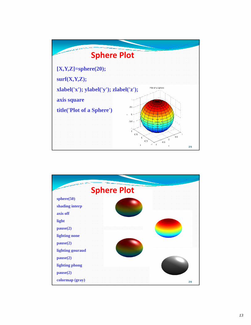
Sphere Plot [X,Y,Z]=sphere(20);
surf(X,Y,Z);
xlabel('x'); ylabel('y'); zlabel('z');
axis square
title('Plot of a Sphere')
25
Sphere Plot sphere(50)
shading interp
axis off
light
pause(2)
lighting none
pause(2)
lighting gouraud
pause(2)
lighting phong
pause(2)
colormap (gray) 26
14
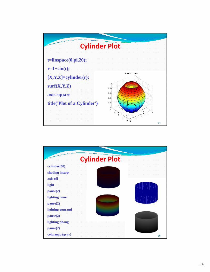
Cylinder Plot
t=linspace(0,pi,20);
r=1+sin(t);
[X,Y,Z]=cylinder(r);
surf(X,Y,Z)
axis squareaxis square
title('Plot of a Cylinder')
27
cylinder(50)
shading interp
Cylinder Plot
axis off
light
pause(2)
lighting none
pause(2)
lighting gouraud
pause(2)
lighting phong
pause(2)
colormap (gray) 28
15
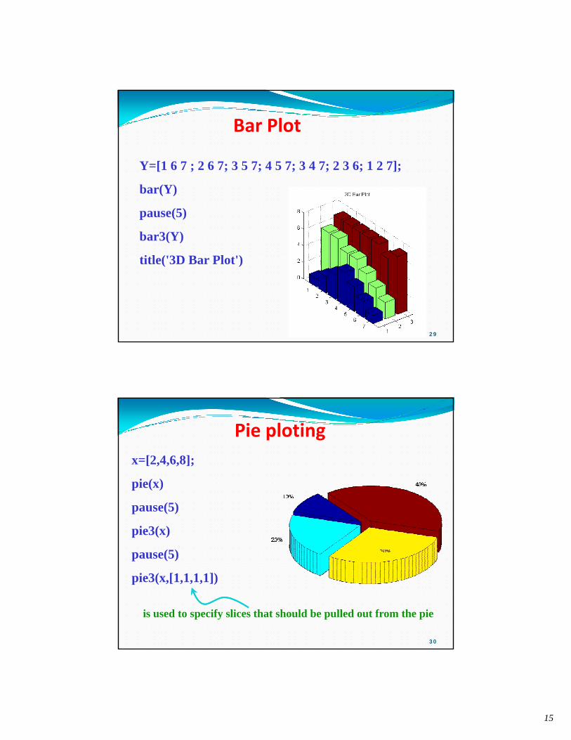
Bar Plot
Y=[1 6 7 ; 2 6 7; 3 5 7; 4 5 7; 3 4 7; 2 3 6; 1 2 7];
bar(Y)
pause(5)
bar3(Y)
title('3D Bar Plot')title('3D Bar Plot')
29
Pie plotingx=[2,4,6,8];
i ( )pie(x)
pause(5)
pie3(x)
pause(5)
pie3(x,[1,1,1,1])
is used to specify slices that should be pulled out from the pie
30
16
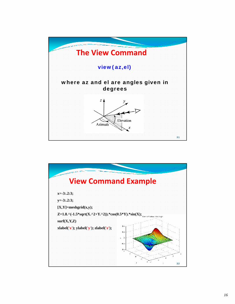
The View Command
view(az,el)
where az and el are angles given in degrees
31
x=-3:.2:3;
View Command Example
y=-3:.2:3;
[X,Y]=meshgrid(x,y);
Z=1.8.^(-1.5*sqrt(X.^2+Y.^2)).*cos(0.5*Y).*sin(X);
surf(X,Y,Z)
xlabel('x'); ylabel('y'); zlabel('z');
32
17
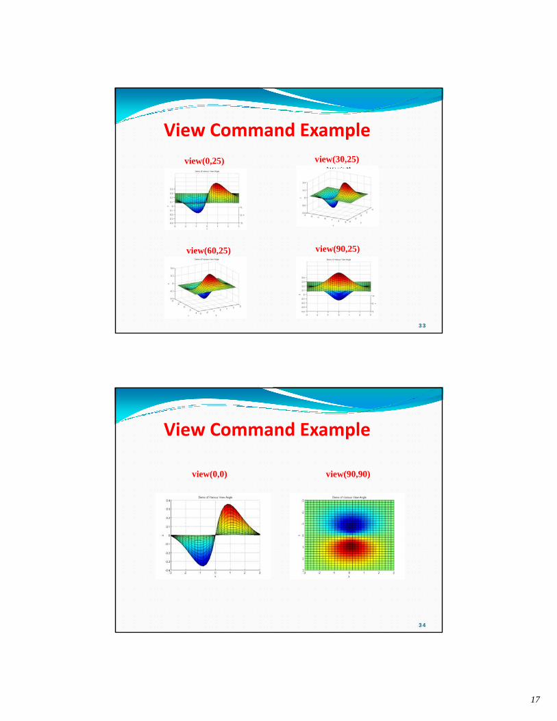
view(0,25) view(30,25)
View Command Example
view(60 25) view(90,25)view(60,25) view(90,25)
33
View Command Example
view(0,0) view(90,90)
34
18
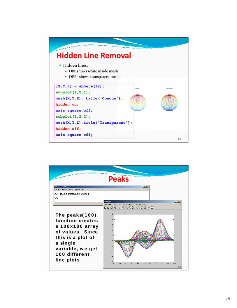
Hidden Line RemovalHidden lines:
ON: shows white inside mesh
[X,Y,Z] = sphere(12);
subplot(1,2,1);
mesh(X,Y,Z), title('Opaque');
hidden on;
OFF: shows transparent mesh
axis square off;
subplot(1,2,2);
mesh(X,Y,Z),title('Transparent');
hidden off;
axis square off;35
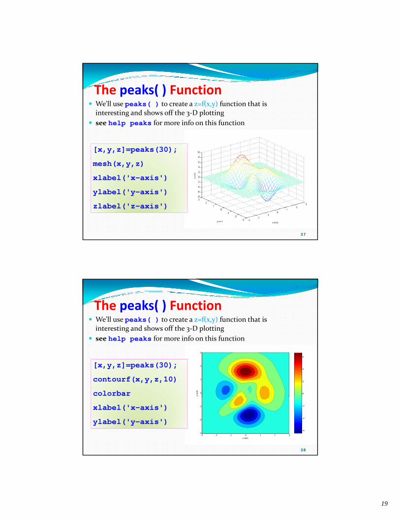
Peaks
The peaks(100) function creates a 100x100 array of values. Since this is a plot of a single variable, we get 100 different line plots
36
19
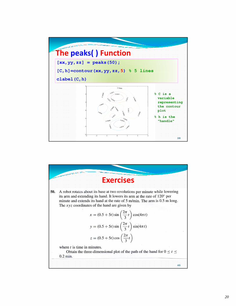
The peaks( ) FunctionWe'll use peaks( ) to create a z=f(x,y) function that is interesting and shows off the 3‐D plottingsee help peaks for more info on this functionsee help peaks for more info on this function
[x,y,z]=peaks(30);
mesh(x,y,z)
xlabel('x-axis')( )
ylabel('y-axis')
zlabel('z-axis')
37
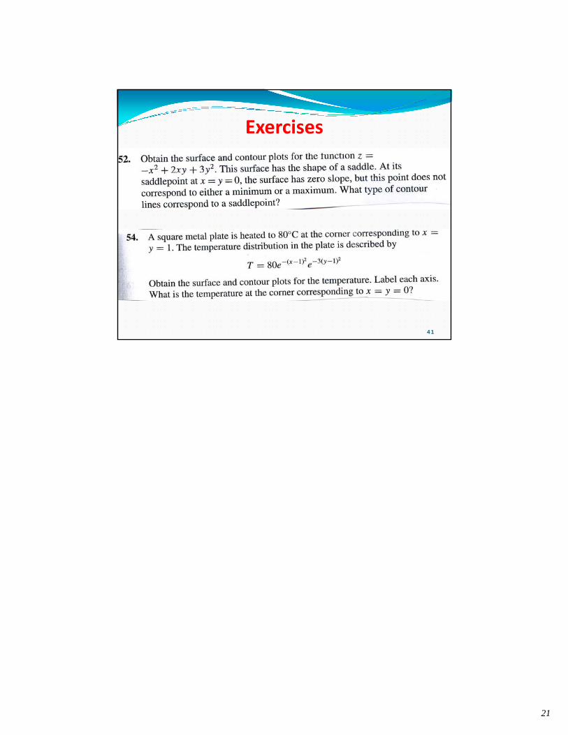
The peaks( ) FunctionWe'll use peaks( ) to create a z=f(x,y) function that is interesting and shows off the 3‐D plottingsee help peaks for more info on this function
0
1
2
3
y-ax
is
0
2
4
6
see help peaks for more info on this function
[x,y,z]=peaks(30);
contourf(x,y,z,10)
colorbar
-3 -2 -1 0 1 2 3-3
-2
-1
x-axis
-6
-4
-2xlabel('x-axis')
ylabel('y-axis')
38
20
The peaks( ) Function[xx,yy,zz] = peaks(50);
[C,h]=contour(xx,yy,zz,5) % 5 lines
1
2
3
-1.6694
5
0.75
885
0.75885
0.75885
3.1871
3.18
713.1871
5.6153
5.6153
[C,h] contour(xx,yy,zz,5) % 5 lines
clabel(C,h)
% C is a variable representing the contour
-3 -2 -1 0 1 2 3-3
-2
-1
0
-4.0976
-4.0976
-1.6694
-1.6694
-1.6694
-1.6694
0.75
885
0.75885
0.75885
0.75885
0.758
85 3.1871
3.187
1
the contour plot
% h is the "handle"
39
Exercises
40
21
Exercises
41