Embed Size (px)
Citation preview
©KHALID AZIZ 2011
Demand, supply and the market

©KHALID AZIZ 2011
JOIN KHALID AZIZ• ECONOMICS OF ICMAP, ICAP, MA-ECONOMICS,
B.COM.• FINANCIAL ACCOUNTING OF ICMAP STAGE 1,3,4
ICAP MODULE B, B.COM, BBA, MBA & PIPFA.• COST ACCOUNTING OF ICMAP STAGE 2,3 ICAP
MODULE D, BBA, MBA & PIPFA.
• CONTACT:• 0322-3385752• 0312-2302870• 0300-2540827• R-1173,ALNOOR SOCIETY, BLOCK 19,F.B.AREA,
KARACHI, PAKISTAN.

©KHALID AZIZ 2011
Join khalid aziz
•FRESH CLASSES• ICMAP STAGE 1,2 & 3•FUNDAMENTALS OF
FA,COST ACCOUNTING ,APPRAISAL & FA
• INDIVIDUAL & GROUPS
©KHALID AZIZ 20114
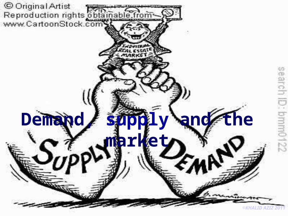
Some key terms• Market
– a set of arrangements by which buyers and sellers are in contact to exchange goods or services
• Demand– the quantity of a good buyers wish to purchase at each
conceivable price
• Supply– the quantity of a good sellers wish to sell at each
conceivable price
• Equilibrium price– price at which quantity supplied = quantity demanded
©KHALID AZIZ 2011
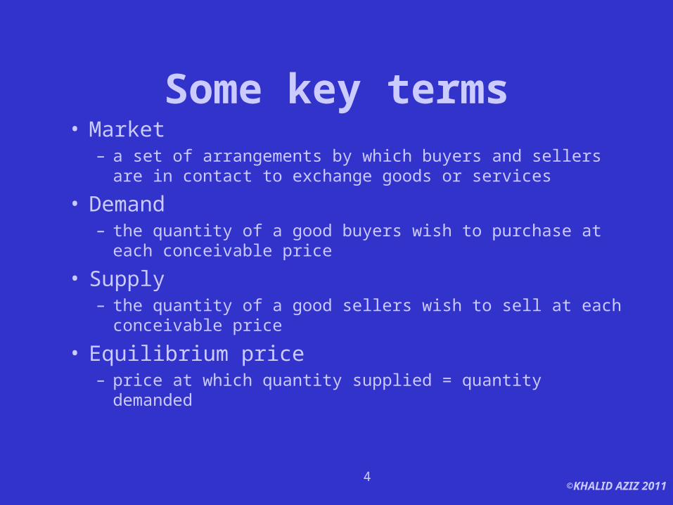
Catherine’s Demand Schedule The demand schedule is a table that shows the
relationship between the price of the good and the
quantity demanded.

©KHALID AZIZ 2011
Figure 1 Catherine’s Demand Schedule and Demand Curve (The demand curve is a graph of the relationship between the price of a good and the quantity demanded.)
Copyright © 2004 South-Western
Price ofIce-Cream Cone
0
2.50
2.00
1.50
1.00
0.50
1 2 3 4 5 6 7 8 9 10 11 Quantity ofIce-Cream Cones
$3.00
12
1. A decrease in price ...
2. ... increases quantity of cones demanded.

©KHALID AZIZ 2011
0
D
Price of Ice-Cream Cones
Quantity of Ice-Cream Cones
A tax that raises the price of ice-cream cones results in a movement along the
demand curve.
A
B
8
1.00
$2.00
4
Changes in Quantity DemandedMovement along the demand curve caused by a
change in the price of the product.

©KHALID AZIZ 2011
Market Demand versus Individual Demand
• Market demand refers to the sum of all individual demands for a particular good or service.
• Graphically, individual demand curves are summed horizontally to obtain the market demand curve.

©KHALID AZIZ 20119
The Demand curve shows the relation between price and quantity
demanded holding other things constant
• “Other things” include:– the price of related
goods– consumer incomes– consumer
preferences• Changes in these other
things affect the position of the demand curve
D
Quantity
Price

©KHALID AZIZ 201110
Prices of related goods and Effect on Demand
Substitute Goods: coffee for tea; train ride for driving your own auto; coal for natural gas
If Price of coffee increases then Demand for tea increases
Complimentary Goods:tea and sugar; coffee and milk; gas and car; coal and coal heaters
If Price of gas increases, then Demand for automobiles decreases

©KHALID AZIZ 201111
Effect of Consumer Income on Demand:
Normal Goods versus Inferior GoodsNormal Goods:
For normal goods, demand increases when consumer income increases.
Most goods are normal goods.
Inferior Goods: For inferior goods, demand decreases when consumer income increases.
Second-hand cars, second-hand clothing, bus rides (versus driving your own auto or cab rides)

©KHALID AZIZ 2011
Ben’s Supply Schedule (The supply schedule is a table that shows the relationship between the price of the good and the quantity supplied.)

©KHALID AZIZ 2011
Figure 5 Ben’s Supply Schedule and Supply Curve (The supply curve is the graph of the relationship between the price
of a good and the quantity supplied.)
Copyright©2003 Southwestern/Thomson Learning
Price ofIce-Cream
Cone
0
2.50
2.00
1.50
1.00
1 2 3 4 5 6 7 8 9 10 11 Quantity ofIce-Cream Cones
$3.00
12
0.50
1. Anincrease in price ...
2. ... increases quantity of cones supplied.

©KHALID AZIZ 2011
Market Supply versus Individual Supply
• Market supply refers to the sum of all individual supplies for all sellers of a particular good or service.
• Graphically, individual supply curves are summed horizontally to obtain the market supply curve.

©KHALID AZIZ 201115
The Supply curve shows the relation between price and quantity supplied
holding other things constant
• “Other things” include:– technology– input costs– government
regulations• Changes in these
other things affect the position of the demand curve
Quantity
Price S
©KHALID AZIZ 2011
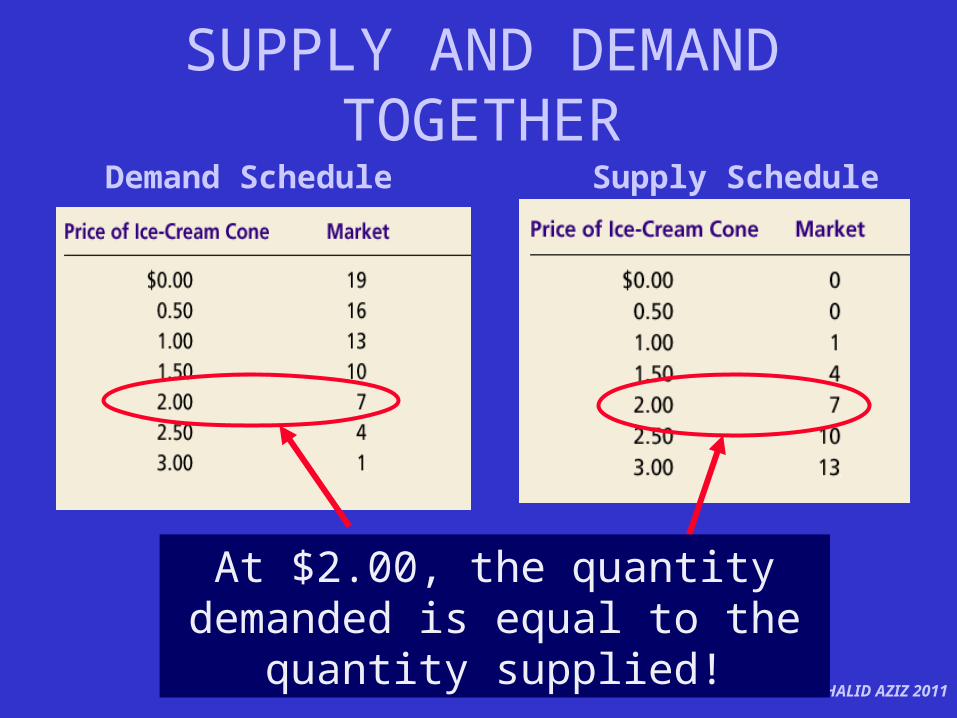
At $2.00, the quantity demanded is equal to the quantity supplied!
SUPPLY AND DEMAND TOGETHER
Demand Schedule
Supply Schedule

©KHALID AZIZ 201117
Market equilibrium (1)
• Market equilibrium is at E0 where quantity demanded equals quantity supplied
D0
D0 S
S
Price
QuantityQ0
P0 E0– with price P0 and
quantity Q0
©KHALID AZIZ 201118
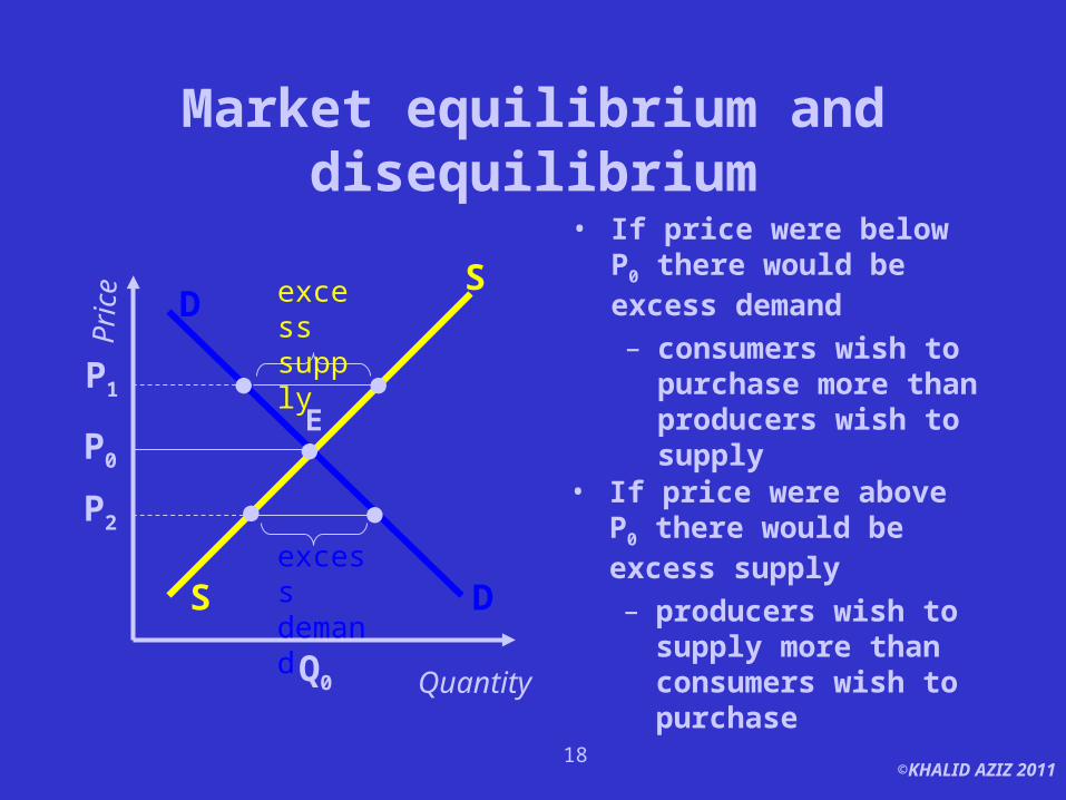
Market equilibrium and disequilibrium
• If price were below P0 there would be excess demand– consumers wish to
purchase more than producers wish to supply
D
DS
S
Q0
P0
E
Price
Quantity
P1
excess supply
P2 excess demand
• If price were above P0 there would be excess supply– producers wish to
supply more than consumers wish to purchase
©KHALID AZIZ 201119
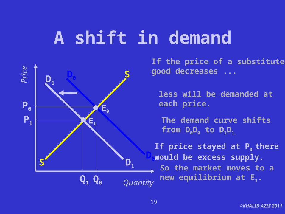
A shift in demand
S
S
E1
Price
Quantity
If the price of a substitute good decreases ...
less will be demanded ateach price.
D0
D0
E0
Q0
P0
The demand curve shiftsfrom D0D0 to D1D1.
D1
D1
Q1
P1
So the market moves to a new equilibrium at E1.
If price stayed at P0 there would be excess supply.

©KHALID AZIZ 201120
A shift in supply
D
D
Q0
P0 E0
Price
Quantity
Suppose safety regulations are tightened, increasing producers’ costs
S0
S0
S1
S1
The supply curve shifts to S1S1
If price stayed at P0 there would be excess demand
Q1
P1
E2
So the market moves to a new equilibrium at E2

©KHALID AZIZ 201121
Two ways in which demand may increase (1)
• (1) A movement along the demand curve from A to B
• represents consumer reaction to a price change
• could follow a supply shift
AP0
Q0 Quantity
Price
D
BP1
Q1

©KHALID AZIZ 201122
Two ways in which demand may increase (2)
• (2) A movement of the demand curve from D0 to D1
• leads to an increase in demand at each price
• e.g. at P0 quantity demanded increases from Q0 to Q2: at P1 quantity demanded increases from Q1 to Q3
A
B
P0
Q0 Q1
D0
Quantity
Price
P1
C
D1
F
Q2 Q3

©KHALID AZIZ 201123
A market in disequilibrium
• Suppose a disastrous harvest moves the supply curve to SS
• government may try to protect the poor, setting a price ceiling at P1
• which is below P0, the equilibrium price level
• The result is excess demand
Quantity
Price
P0
Q0QS
DS
P1
E
A B
P2
excess demand
QD
D S
RATIONING is needed to cope with the resulting excess demand

©KHALID AZIZ 201124
Price and quantity changes
• In practice, we cannot plot ex ante demand curves and supply curves
• So we use historical data and the supposition that the observed values are equilibrium ones
• Since other things are often not constant, some detective work is required
• This is where our theory comes in useful

©KHALID AZIZ 201125
What, how and for whom
• The market:– decides how much of a good should be produced
• by finding the price at which the quantity demanded equals the quantity supplied
– tells us for whom the goods are produced• those consumers willing to pay the equilibrium price
– determines what goods are being produced• there may be goods for which no consumer is prepared
to pay a price at which firms would be willing to supply

©KHALID AZIZ 2011
JOIN KHALID AZIZ• ECONOMICS OF ICMAP, ICAP, MA-ECONOMICS,
B.COM.• FINANCIAL ACCOUNTING OF ICMAP STAGE 1,3,4
ICAP MODULE B, B.COM, BBA, MBA & PIPFA.• COST ACCOUNTING OF ICMAP STAGE 2,3 ICAP
MODULE D, BBA, MBA & PIPFA.
• CONTACT:• 0322-3385752• 0312-2302870• 0300-2540827• R-1173,ALNOOR SOCIETY, BLOCK 19,F.B.AREA,
KARACHI, PAKISTAN.