Embed Size (px)
Citation preview

0
Yield Curve Premia
JORDAN BROOKS AND TOBIAS J. MOSKOWITZ∗
Preliminary draft: January 2017 Current draft: July November 2017
Abstract
We examine return premia associated with the level, slope, and curvature of the yield curve over time and across countries from a novel perspective by borrowing pricing factors from other asset classes. Measures of value, momentum, and carry, when applied to bonds, provide a rich description of bond return premia: subsuming pricing information from the yield curve’s first three principal components, as well as priced factors unspanned by yield information, such as macroeconomic growth, inflation, and the Cochrane and Piazzesi (2005) factor. These characteristics provide new economic intuition for what drives bond return premia, where value, measured by a bond’s yield relative to a fundamental anchor of expected inflation, subsumes a “level” factor. Momentum, which reveals recent yield trends, and carry, which captures expected future yields if the yield curve does not change, subsume information about expected returns from the slope and curvature of the yield curve. These characteristics describe both the cross-section and time-series of yield curve premia and connect to return predictability in other asset classes, suggesting a unifying asset pricing framework.
∗Brooks is at AQR Capital, email: [email protected] and Moskowitz is at Yale SOM, Yale University, NBER, and AQR Capital, email: [email protected]. We thank Cliff Asness, Attakrit Asvanunt, Paolo Bertolotti, Andrea Eisfeldt, Antti Ilmanen, Ronen Israel, Michael Katz, John Liew, Lasse Pedersen, Monika Piazzesi, Scott Richardson, Zhikai Xu, and seminar participants at the NBER Asset Pricing Summer Institute for valuable comments. We also thank Paolo Bertolotti and Anton Tonev for outstanding research assistance. Moskowitz thanks the International Finance Center at Yale University for financial support.

1
What drives expected returns of assets in the economy? This central question in asset pricing has
received much attention, where the literature has propagated seemingly different models for different
asset classes. Government bonds in particular have often evolved their own, seemingly separate set
of factors, largely motivated by affine models that describe yields (due to their lack of cash flow risk
and very strong factor structure). In other asset classes, such as equities, expected returns are often
described by empirical characteristics such as value, momentum, and carry.1
An essential element of all asset pricing models, however, is the level and dynamics of the
riskless rate of interest. Hence, connecting return predictors across asset classes, particularly
government bonds, should be a primary goal of asset pricing research. Attempts to explain return
predictability through macroeconomic risks offer a general connection across asset classes, but with
limited success. We take a more direct approach by applying return predictors ubiquitous in other
asset classes to the yield curve to potentially identify links across asset class return premia that help
improve our understanding of what drives asset price dynamics in the global economy.
We seek two main objectives. The first is to better understand the return premia associated
with the term structure of interest rates, both over time and across geographies (countries). Are the
same factors that describe cross-maturity variation in yields the ones that drive return premia, as the
structure of unrestricted affine models predict? Do the same predictors for time-variation in a single
asset’s expected return also explain the international cross-section of expected returns? The second
goal is to link yield curve return premia to those from other asset classes. Are there connections to
return predictors from equity and other markets that help explain bond returns? How do these return
predictors relate to traditional bond market yield factors and unspanned sources of returns? Both
goals serve to improve our understanding of asset pricing specific to government bonds and, more
generally, to connect return premia across diverse assets.
Most of the evidence on bond risk premia comes from U.S. Treasuries focusing on time-
variation in expected returns, and the more limited international evidence supports the U.S. findings.2
We expand the sample of international bond markets and look at both the time series and cross-
section of government bond returns. Using both data on international zero coupon rates with 1 Value, momentum, and carry characteristics have been shown to price assets in equities (Jegadeesh and Titman (1993), Fama and French (1996, 2012), Asness, Moskowitz, and Pedersen (2013)), equity indices, fixed income, currencies, commodities, and credit (Asness, Moskowitz, and Pedersen (2013), Koijen, Moskowitz, Pedersen, and Vrugt (2016), Asness, Ilmanen, Israel, and Moskowitz (2015), Israel, Palhares, and Richardson (2016)). 2 A well-cited but non-exhaustive list for US treasuries includes Fama and Bliss (1987), Campbell and Shiller (1991), Bekaert and Hodrick (2001), Dai and Singleton (2002), Dai, Singleton, and Yang (2004), Gürkaynak, Sack, and Wright (2007), Cochrane and Piazzesi (2005, 2008), Wright (2011), Joslin, Priebsch, and Singleton (2014), Bauer and Hamilton (2015), Cochrane (2015) and Cieslak and Povala (2017). International evidence can be found in Kessler and Scherer (2009), Hellerstein (2011), Sekkel (2011), and Dahlquist and Hasseltoft (2015).

2
synthetically constructed returns (as is standard in the literature), as well as a unique sample of
international tradeable bonds with live returns, we investigate the drivers of return premia across
countries and maturities, and assess whether the same variables that drive time-variation in expected
returns also explain the cross-section of expected returns. In addition to looking at the level of the
yield curve, which the literature almost exclusively focuses on,3 we examine return premia associated
with the slope and curvature of the yield curve, where the 10-year bond, the difference between the
10- and 2-year bonds, and the difference between the 5- and an average of the 2- and 10-year bonds
represents our “level”, “slope”, and “butterfly” portfolios, respectively.
We first consider traditional bond market factors, such as the first three principal
components (PCs) of the yield curve motivated by affine term structure models. We then consider a
set of factors not commonly used to price bonds, but used extensively to describe returns in other
asset classes – “style” factors or characteristics related to value, momentum, and carry. We show that
these style characteristics capture the time-series and cross-section of yield curve premia better than
the PCs, despite the first three PCs describing nearly all (99.9%) of the variation in yields across
maturities in every country and being highly correlated across countries. The first PC, which captures
the average level of yields across maturities, forecasts returns to the level portfolios through time,
consistent with the literature (Cochrane and Piazzesi (2005, 2008), Joslin, Priebsch, and Singleton
(2014)), but also captures returns across countries. The second PC, related to the slope of the yield
curve, has predictive power for both the level and slope portfolios across countries, and the third PC,
related to the curvature of the yield curve, forecasts the returns to the butterfly portfolios. Adding the
style characteristics value, momentum, and carry, however, we find significant style return premia
for all three categories of bond portfolios (level, slope, and butterfly), even after controlling for the
principal components that fully describe all cross-maturity variation in the yield curve. The styles
pick up significant unspanned pricing information. But perhaps most intriguing, is that the styles also
subsume the pricing information from the PCs, capturing information from the yield curve as well.
We use measures of value, momentum, and carry from the literature, where value is the yield
on the bond minus (maturity-matched) expected inflation (“real bond yield”), momentum is the past
12-month return on the bond (both used by Asness, Moskowitz, and Pedersen (2013)), and carry is
defined similar to Koijen, Moskowitz, Pedersen, and Vrugt (2016), as the “term spread,” or the yield
on the bond minus the local short rate. There is a natural economic interpretation to these style
characteristics that relates to yields in an intuitive way. Value, measured by the real bond yield, 3 Duffee (2011) is the lone exception, who looks at time-variation in expected returns for the slope of US treasuries, but does not look at cross-sectional, international, or curvature returns.

3
provides information about the level of yields in relation to a fundamental anchor – expected
inflation; momentum provides information about recent trends in yield changes; and carry provides
information about expected future yields assuming the yield curve stays the same. For example, for
the level portfolios across countries, value strategies are long high real yield countries and short low
real yield countries, which is a profitable strategy if yields revert to fundamental levels, like expected
inflation. Momentum strategies will be profitable if recent yield changes continue in the same
direction, and carry strategies will be profitable if the current yield curve stays approximately the
same. Consistent with this interpretation, we find that value subsumes the pricing information from
the first principal component of the yield curve, but also provides additional explanatory power
because inflation expectations seem to matter, too, for expected returns. Bond pricing seems to
depend more on the level of yields relative to some fundamental anchor rather than simply the
absolute level of yields. Carry subsumes information from the second principal component, tied to
the slope of yields, and although momentum’s explanatory power for returns by itself is weak, the
combination of value, momentum, and carry subsumes the information in the third PC.
While the cross-sectional evidence of style premia for level portfolios is consistent with
Asness, Moskowitz, and Pedersen (2013) and Koijen, Moskowitz, Pedersen, and Vrugt (2016), the
time-series evidence and the evidence of style premia for slope and butterfly portfolios is novel.
Moreover, the style characteristics subsume the cross-sectional and time-series pricing information
from the PCs and provide additional explanatory power for return premia.
Since the style factors are not spanned by the PCs yet appear to contain incremental
information about excess returns, we also consider other “unspanned” sources of returns from the
literature, such as output growth and inflation (Joslin, Priebsch, and Singleton (2014), Bauer and
Hamilton (2015), and Cochrane (2015)), the Cochrane and Piazzesi (2005, CP) factor, a tent-shaped
linear combination of forward rates, and the cycle factor of Cieslak and Povala (2017). While
evidence on these unspanned factors is generally confined to the U.S. time series, we examine them
in an international context, allowing us to test their efficacy in explaining the cross-section of
government bond returns as well. Unspanned macroeconomic factors price assets across countries
similar to the time-series evidence shown in the U.S. We also find evidence consistent with Cochrane
and Piazzesi (2005) that a single factor constructed from forward rates captures time-varying
expected returns in each of our international bond markets. However, we also show that the
explanatory power of these variables is subsumed by the style factors, and that the styles continue to
provide additional pricing information beyond these sources, even in the presence of the PCs.

4
The style characteristics provide additional intuition for what drives bond returns. For
example, Joslin, Priebsch, and Singleton (2014) and Bauer and Hamilton (2015) show that inflation
is a statistically significant forecaster of bond level excess returns in the presence of the PCs. We
confirm that finding internationally, but when adding the value factor, we find it subsumes the
explanatory power of inflation for pricing. This finding is consistent with Cochrane’s (2015)
conjecture that inflation’s predictive power derives essentially from providing a baseline or “anchor”
from which to compare yields. We also show that the Cochrane-Piazzesi (CP) factor, which prices
bonds over time in each international market we study, is also captured by our value measure. The
intuition is that the CP factor picks up future pricing information from forward rates that seem to be
well represented by the concept of value – the level of yields relative to expected inflation.
Consistent with this interpretation, Cieslak and Povala (2017) decompose bond premia into two
components: expected inflation and variation in yields unrelated to expected inflation, which they use
to form their “cycle factor” that also captures the CP factor. This factor is an average of 2- to 20-year
maturity bonds minus the short rate, which is very similar to our value factor.
Importantly, however, our style factors do not just subsume these other factors and relabel
them, but provide additional explanatory power for return premia beyond these other factors.
Moreover, while the macro, CP, and cycle factors are only used to explain the time-series of level
returns (in the U.S.), we show that the concepts of value, momentum, and carry also capture cross-
sectional return premia in levels, slope, and curvature of the yield curve. Taken together, the three
style characteristics value, momentum, and carry deliver a better and more comprehensive fit for
yield curve premia in general, explaining more of the time-series and cross-sectional variation in
bond level returns than the PCs and other unspanned sources of returns found in the literature, and
also capturing return premia associated with the slope and curvature of the term structure.
We also apply these style concepts to unique data on live tradeable bonds across 13 countries,
which allows us to 1) calculate actual returns that address possible measurement issues with synthetic
zero coupon returns commonly used in the literature, 2) provide an out of sample test of the various
predictors of bond returns found here and in the literature, and 3) relate bond style returns to style
returns from other asset classes. We find that real-time level, slope, and butterfly trading strategies
for value, momentum, and carry indeed deliver positive abnormal returns. We also find positive
correlation among value strategies and among carry strategies across the level, slope, and butterfly
portfolios, indicating that their returns share common variation across the yield curve.
In addition to providing stronger return predictability and further intuition for what drives
yield curve premia, another virtue of the style factors is that they directly connect to asset pricing

5
factors from other asset classes. Using the live bond return data we find a significant positive relation
between style premia in government bond level returns and style premia in other asset classes. Value,
momentum, and carry in government bonds share common variation with value, momentum, and
carry in other asset classes, hinting at a common framework linking return predictability across asset
classes. Such a link adds to a growing list of empirical facts suggesting that these styles represent
common sources of return premia across many asset classes (Asness, Moskowitz, and Pedersen
(2013), Fama and French (2012), Koijen, Moskowitz, Pedersen, and Vrugt (2016), Zaremba and
Czapkiewicz (2016)), including fixed income, which has largely eschewed these factors.4
Our results have important implications for asset pricing theory. Our evidence suggests a new
framework for thinking about yield curve return premia, but one that is commonly used to describe
return premia in many other asset classes. However, while a simple style factor model appears to be a
good and parsimonious empirical description of return premia, much theoretical debate remains on
the underlying economic drivers of these style premia. Whether return premia associated with these
characteristics are driven by unknown sources of risk or by mispricing from correlated investor
behavior remains an open question. Nevertheless, their connection across diverse asset classes seems
to be an important feature for any theory to accommodate, including fixed income models that have
previously appeared “disconnected” from other asset classes.
The rest of the paper is organized as follows. Section I describes the international bond data
and the variation in yields and returns. Section II examines the cross-section and time-series of
expected returns across maturities and countries, and how they relate to affine factors and style
characteristics. Section III considers unspanned sources of returns and how they relate to the style
factors. Section IV constructs portfolios of tradeable bonds based on the style characteristics and
examines their commonality across moments of the term structure and across different asset classes.
Section V concludes with a discussion of the implications of our findings for asset pricing theory.
I. International Bond Data and Yield Curves
We describe the set of zero coupon yields we use across countries and present summary statistics on
their implied yield curves. We also describe our data on tradeable bonds.
A. Zero Coupon Yield Data
4 Zaremba and Czapkiewicz (2016) examine the cross-section of government bond returns internationally using a shorter but broader sample of bonds from developed and emerging markets, where they find that a four factor model based on volatility, credit, value, and momentum explains bond returns well. They make no attempt, however, to connect these factors to other yield curve dynamics or other bond factors in the literature, nor do they connect their factors to those from other asset classes.

6
We examine zero curves for seven international government bond markets: Australia, Germany,
Canada, Japan, Sweden, UK, and US. The data come from Wright (2011) and can be downloaded
from Jonathan Wright’s website http://econ.jhu.edu/directory/jonathan-wright/. The data are
monthly, but we aggregate yields to quarterly to mitigate the influence of data errors or liquidity
issues. The zero coupon yields begin at various dates per country and end in May 2009.5
We supplement Wright’s (2011) data, with bond price data from Reuters DataScope Fixed-
Income (DSFI) database, obtained from AQR Capital, to provide yields from June 2009 to March
2016. The bond prices are checked and consolidated using secondary sources such as Bloomberg.
Although Wright’s (2011) data also covers Switzerland, Norway, and New Zealand, due to the small
number of issuances of bonds from those countries post-2009, we drop those three countries from our
database and hence have seven countries with zero coupon yields across maturities from 1 to 30
years dating as far back as December 1971 through March 2016.6
To form yields from the DSFI database, we first group bonds in each country into different
tenors (2, 3, 5, 7, 10, 15, 20, 30) by their time-to-maturity as of their most recent issuance. We
remove the newly issued bond for each tenor as well as the aged ones (e.g., a 7-year bond having a
time to maturity shorter than any of the 5-year bonds). We then apply a bootstrap procedure for the
bonds with linear forward rate interpolation using a set of liquid bonds which span the full curve to
obtain zero curves. While we exclude the aged illiquid bonds based on issuance and re-issuance
calendars, we do not smooth the curves after bootstrapping. From the zero-coupon yields we take log
yields and compute log forward rates and quarterly log returns (annualized) in excess of the three-
month yield following Cochrane and Piazzesi (2005).
B. Summary Statistics
Figure 1 plots the mean and standard deviation of yields to zero-coupon bonds by country
corresponding to maturities of one to ten years. Average (log) yields vary across maturities within 5 The data sources and methodology used by Wright (2011) to compute zero coupon yields are: Country Start Date Source Methodology Australia 3/31/1987 Datastream and Wright's calculations Nelson-Siegel Germany 3/30/1973 Bundesbank and BIS database Svensson Canada 3/31/1986 Bank of Canada and BIS database Spline Japan 3/29/1985 Datastream and Wright's calculations Svensson Sweden 12/31/1992 Riksbank and BIS database Svensson UK 3/30/1979 Anderson and Sleath (1999) Spline US 12/31/1971 Gürkaynak, Sack, and Wright (2007) Svensson 6 In the appendix, we provide a set of our main results including these three countries despite their small number of issuances and show that the results are quantitatively similar.

7
each country and vary substantially across countries. The slopes of yields across maturities also vary
by country. The second plot in Figure 1 graphs the mean and standard deviation of total returns,
where there is more variation across maturities and countries.
For each country, we extract the first three principal components (PCs) of the yield curve
(from maturities 1 through 10). Panel A of Table I reports the fraction of the covariance matrix of
yields across maturities in each country explained by each of the first three PCs as well as the total
amount of variation explained by all three PCs. The first three PCs capture nearly all of the variation
in yields across maturities within each country, capturing a minimum of 99.7% (CN) to 99.9% (AU)
of yield variation, a fact first documented in U.S. data by Litterman and Scheinkman (1991).
Figure 2 plots the loadings of each bond on the principal components in each country. The
first plot shows the loadings for the first PC across countries, which captures the level of interest
rates. The second plot shows loadings on the second PC, which uniformly seems to capture the slope
of the yield curve, and the third plot shows that loadings on the third PC exhibit a hump-shaped
pattern, with negative loadings on the short and long-term yields and positive loadings on
intermediate horizon yields, capturing some of the “curvature” of the yield curve. The patterns of all
three PCs are similar across countries, with some variation in the coefficients for PC3.
Figure 3 plots the quarterly time series of each PC for each country over time. The first plot
shows that PC1 is highly correlated across countries, averaging 0.94, with most pairwise correlations
above 0.90. The second plot shows the time series variation in PC2, which is also fairly highly
correlated across countries, averaging 0.44. The third plot shows the results for PC3, which is the
least correlated across countries, but still has an average pairwise correlation of 0.27.
C. Level, Slope, and Curvature Portfolios
We wish to understand the factors that drive the dynamics of the yield curve over time and across
countries. We focus on forecasting excess returns to three simple portfolios designed to span most of
the economically interesting variation in the yield curve. The first portfolio is a “level” portfolio that
consists simply of the 10-year bond in each country. The second portfolio is a“slope” portfolio that is
long the 10-year bond and short the 2-year bond, adjusted to be duration neutral. The third portfolio
is a “curvature” or “butterfly” portfolio that is long the 5-year bond and short an equal-duration
weighted average of the 2- and 10-year bonds in each country.
We use these simple portfolios to concisely represent the moments of the yield curve based
on the first three principal components of the yield curve capturing virtually all economically
meaningful variation across maturities. We form these portfolios rather than use the PCs themselves

8
because PC weights change over time and can overfit each time period’s yield curve, whereas our
simple portfolios weights remain constant and economically intuitive.7 Essentially, we reduce the
information from each country’s yield curve into these three portfolios due to the strong factor
structure in yields, allowing us to parsimoniously examine yield dynamics.
Highlighting the ability of these portfolios to represent the moments of the yield curve, Panel
B of Table I reports the correlations between the PCs and the yields on the level, slope, and butterfly
portfolios. The first row reports the correlation between PC1 and the yield on the level portfolio by
country, which is 1.00 for every country in our sample. The second row reports the correlations
between PC2 and the yield on the slope portfolio, which ranges from 0.84 (US) to 0.98 (AU, JP, SD)
and averages 0.94. The third row reports correlations between PC3 and the yield on the butterfly
portfolio for each country, which ranges from 0.73 (BD, CN) to 0.98 (UK) and averages 0.85. Hence,
the three portfolios are highly correlated to the principal components.
Panel A of Table II reports the mean, standard deviation, and t-statistic of the yields for the
level, slope, and curvature portfolios in each country, and Panel B reports summary statistics for their
excess returns across countries. The average correlation of excess returns among the level portfolios
is 0.65, smaller than that obtained for yields, which is intuitive since excess returns are driven in part
by changes in yields. For perspective, the average correlation of the excess returns to each of our
country’s value-weighted aggregate equity market portfolio is around 0.60 over the same time period.
For the slope portfolios’ excess returns, we find wide variation across countries, but also positive
correlation of 0.38 on average, slightly lower than the average correlation in yields (0.46). For the
butterfly portfolios, excess returns also vary widely, but the correlations of excess returns across
countries are 0.25 on average, which again is only slightly lower than the average yield correlation.
Tables I and II show that the yields on level, slope, and curvature portfolios across countries
mirror the first three principal components from each country, where yields and returns of each
dimension of the yield curve are positively correlated across countries, but also exhibit substantial
cross-sectional variation. We seek to understand the time-series and cross-sectional variation in
excess returns for each of the three dimensions of the yield curve across countries.
D. Tradeable Bond Universe
7 Alternatively, we could have taken an equal-weighted average of all maturities for the level portfolio, or used an average of long-end bonds minus short-end bonds for the slope, or similarly taken an average of intermediate horizon bonds minus an average of long and short-end bonds for curvature. All of our results are consistent with various portfolios that capture the same information from the yield curve, which given the strong factor structure of yields across maturities is not surprising.

9
In addition to analyzing the set of zero-coupon yields, where we calculate synthetic returns, we also
examine a set of tradable bonds covered by the JP Morgan Government Bond Index (GBI) to provide
a set of live returns on tradeable portfolios. These data address any concerns of return mis-
measurement, offer a broader cross-section of bonds, provide a new sample test, and generate returns
that can be compared to other asset classes.
The JPM GBI contains a broader cross-section of markets, but a more limited time series than
our zero coupon data. Specifically, it contains a market cap weighted index of all liquid government
bonds across 13 markets: Australia (AU), Belgium (BD), Canada (CN), Denmark (DM), France (F),
Germany (GR), Italy (IT), Japan (JP), Netherlands (ND), Spain (SP), Sweden (SD), the United
Kingdom (UK), and the United States (US), excluding securities with time to maturity less than 12
months, illiquid securities, and securities with embedded optionality (e.g., callable bonds).
The data is sub-divided into country-maturity partitions, where bonds with 1-5 year time-to-
maturity (TTM), 5-10 year TTM, and 10-30 year TTM are grouped. For each maturity bucket, JP
Morgan provides total returns (we dollar hedge all returns), duration, average TTM, and yield to
maturity. In our analysis we take these country-maturity groups to be our primitive assets. The assets
that form the basis of our portfolios in Section IV are portfolios of liquid, underlying bonds within
the above three maturity buckets within each of the 13 countries, producing 3x13 = 39 test assets.
E. Macroeconomic Data
We also use macroeconomic data on expected inflation and output growth from Consensus
Economics. Expected inflation is used in the construction of real bond yield measures, while both
expected inflation and output growth are used as potential unspanned macroeconomic factors. CPI
inflation forecasts are for the current year and the subsequent ten years, and are median forecasts
across a panel of respondents. Output growth is the percent change in industrial production over the
next year, and likewise is the median across the panel of respondents. Consensus forecasts begin in
1990. Prior to 1990, we use realized year-on-year inflation and industrial production growth (both
from Datastream) as proxies for expected inflation and output growth. To account for reporting lags,
we lag each series by an additional quarter.
II. The Cross-Section and Time-Series of Yield Curve Premia
We begin by examining the cross-section of level returns, and then proceed to the cross-section of
slope and butterfly returns across countries. As argued previously, these three portfolios characterize
all yield-maturity variation, reducing the number of parameters to be estimated, and lend themselves

10
easily to portfolio formation to match the live bond portfolio data in Section IV. We then examine
time-series variation in level, slope, and butterfly returns.
A. Yield Curve Factors and the Cross-Section
The first column of Panel A of Table III reports results from predictive regressions of quarterly
excess returns of the cross-section of country government bonds on the first three principal
components of the yield curve from the previous quarter. The dependent variable in Panel A is the
excess return on the level portfolio in each country (10-year maturity bond return in excess of the 3-
month short rate) in quarter t+1. To isolate the cross-sectional differences in returns across countries,
we include time fixed effects in the regression. Formally, the regression equation is,
rtt
Levelt PCBrx 11 F.E. Time ++ ++′= ε (1)
where rxLevelt+1 is the excess return on the 10-year bond in each country. We compute t-statistics that
account for cross-correlation of the residuals.
As the first column of Panel A of Table III shows, the first two principal components are
significantly positively related to future average returns of the level portfolios in each country. The
positive coefficients imply that a relatively high average yield (PC1) and a relatively steep curve
(PC2) jointly predict higher 10-year bond excess returns in the country over the next quarter.
B. Style Factors and the Cross-Section
The PC factors are motivated by affine models that (implicitly) assume the same factors that drive
cross-maturity variation in yields also drive time series variation in excess returns. Since the first
three PCs capture 99.9% of the cross-maturity variation in yields, the PCs should be sufficient for
describing expected returns according to these models. Other models can give rise to factors not
contained in yields driving bond risk premia, consistent with the empirical findings of Cochrane and
Piazzesi (2005), Ludvigson and Ng (2010), Duffee (2011), and Joslin, Priebsch, and Singleton
(2014). In this subsection, we examine a set of factors motivated by asset pricing models from other
asset classes. Specifically, we look at empirical characteristics that explain expected returns in many
other asset classes: value, momentum, and carry, which capture expected returns in equities, fixed
income, credit, currencies, commodities, and options (Asness, Moskowitz, and Pedersen (2013),
Fama and French (2012), and Koijen, Moskowitz, Pedersen, and Vrugt (2016)).
To measure value, momentum, and carry we use the simplest, and to the extent a standard
exists, most standard indicators of each. For value, we use the “real bond yield,” which is the

11
nominal yield on the bond minus a maturity-matched CPI inflation forecast from Consensus
Economics as described previously. The idea behind this measure is to capture the relative valuation
of a bond by comparing its current yield to expected inflation, which compares the bond’s current
market value to a “fundamental” anchor. This measure is similar in spirit to examining the ratio of a
stock’s fundamental value (such as its book equity) to its market value, which the literature studying
equity risk premia has used as its chief value indicator (Fama and French (1992, 1993, 1996, 2012),
Asness, Moskowitz, and Pedersen (2013), and many others). For momentum, we use the one-year
past return on the bond, which has become the standard price momentum measure used in equities
and other asset classes (Asness, Moskowitz, and Pedersen (2013)). Finally, for carry we use the term
spread or 10-year yield minus the local short (3-month) rate similar to Koijen, Moskowitz, Pedersen,
and Vrugt (2016).8 The idea behind this measure is to define carry as the return an investor receives
if market conditions remain constant; in this case assuming the yield stays the same.
The second through fourth columns of Panel A of Table III report univariate forecasting
regression results of the time t+1 excess bond return across countries on each of the style
characteristics just defined – value, momentum, and carry. The results indicate that both carry and
value capture significant and positive risk premia in the cross-section of government bond returns,
with carry having a 0.25 coefficient (t-stat = 2.11) and value a 0.53 coefficient (t-stat = 3.56).
However, momentum does not exhibit a significant risk premium. We later assess the economic
magnitude of these results by looking at live portfolios of value, carry, and momentum.
Column (5) reports the multivariate results when all three style characteristics are included in
the regression. Here, both carry and value remain positive and actually increase in significance (carry
having a coefficient of 0.30 with a t-stat = 2.64 and value having a coefficient of 0.50 with a t-stat =
3.72), which suggests that carry, value, and momentum are diversifying and complement rather than
subsume each other. Momentum remains insignificant and actually has a negative point estimate.
Comparing column (5), which uses the three style characteristics, to column (1), which uses
the principal components, the R-square is substantially larger for the styles than the PC factors. The
styles capture more of the cross-sectional variation in bond expected returns than the PCs, even
8 Koijen, Moskowitz, Pedersen, and Vrugt (2016) define carry as the (synthetic) futures excess return assuming market conditions – the yield curve – stays the same. Under this definition, carry is the term spread plus the “roll down” component of the yield curve as the bond approaches maturity. We simply use the term spread as our measure of carry because we do not have a simple yield curve of our tradeable bond portfolios to compute the roll down component. However, in the appendix we approximate the roll down component using our tradeable bonds sample and the zero coupon yields and show that this component has a negligible effect on the results.

12
though the PCs span nearly all of the variation in yields across maturities. Below we conduct a
formal test comparing the explanatory power of the style characteristics versus the affine factors.
Columns (6) through (8) of Panel A examine each style factor in conjunction with the three
principal components, by adding the style characteristics to equation (1):
rttttt
Levelt Mom CarryValSPCBrx 11 F.E. Time][ ++ ++′+′= ε . (2)
Both value and carry remain significantly positive (and momentum insignificant) even in the
presence of the three PCs. Looking at the coefficients on the PCs, it appears that PC1 is subsumed by
value, dropping from a significant coefficient of 0.089 (t-stat = 2.63) to an insignificant coefficient of
0.039 (t-stat = 1.05) in the presence of value. However, PC2 remains significant in the presence of
value. Carry, on the other hand, seems to completely subsume PC2, whose coefficient drops from
0.254 (t-stat = 2.42) to 0.015 (t-stat = 0.08) when carry is added, but has little effect on PC1.
Momentum, which does not appear related to the cross-section of country-level returns, does not
affect any of the PCs. Finally, the last column of Panel A of Table III (column (9)) reports the full
forecasting regression that includes all three PCs and all three styles. The results confirm and
summarize our findings: significant positive risk premia associated with value and carry exist that
seem to subsume the information in expected returns coming from the principal components of the
yield curve, where value captures PC1 and carry captures PC2. The last row of Panel A reports the p-
value of a nested F-test that tests whether the additional style factors add significant explanatory
power beyond the principal components. The test soundly rejects the null that the principal
components are sufficient descriptors of bond risk premia in favor of a model that includes these
style characteristics.9
C. Cross-Section of Slope Returns
Panel B of Table III examines the slope returns across countries by repeating the regressions above,
but using the excess returns on the slope portfolio in each country instead of the level returns.
Specifically, we run the following regression,
rttttt
Slopet Mom CarryValSPCBrx 11 F.E. Time][ ++ ++′+′= ε , (3)
where rxSlopet+1 is the excess return to the slope portfolio in each country, which is the 10-year bond
minus the 2-year bond , where we adjust for duration of the two bonds. Forecasting duration-neutral
9 Our results are nearly identical if we define the level portfolio for each country as the average yield across all maturity bonds (1 – 10 years) within the country – where we weight the bonds equally or by constant duration or by liquidity – or simply use the 5-year bond in each country instead of the 10-year bond to define levels, or use the 2-year bond to define country levels.

13
slope returns is essentially equivalent to forecasting the change in the slope of the yield curve. Hence,
the duration adjustment simply isolates the change in slope separately from any change in levels,
making these set of portfolios largely independent from the level portfolios we already examined.
Value for the slope portfolio in each country is simply the difference in real bond yields
between the 10-and 2-year bonds, and carry is the difference in yields relative to the short-rate
between the two bonds, where we adjust for duration. Since value is about yield convergence we do
not duration-adjust (a duration adjustment would have no impact on the signal). For carry, however,
the duration adjustment is economically important because carry is essentially a return (difference in
yields) assuming the yield curve does not change, and we want to model the carry on the portfolio of
bonds whose returns we are actually predicting. For the same reason, we will also make our
momentum measure duration neutral so that the past duration-neutral return is used to forecast the
future duration-neutral return. Specifically, the style measures for slope returns are therefore:
)])2([()])10([(Value 210 iEyiEy ty
tty
tSlopet −−−= (4)
)(2
)(10
Carry .32.310 mot
yt
mot
yt
Slopet yyDyyD
−−−= (5)
)(2
)(10
Mom 21,12
101,12
ytt
ytt
Slopet retDretD
−−−− −= (6)
where ytn is the yield at time t on the n-maturity government bond, Et[i(n)] is expected inflation at
time t for horizon n, and retnt-12,t-1 is the past 12-month return on the n-maturity bond. The duration
adjustment scales all durations to a constant D years, where we arbitrarily set D = 10.
As the first column of Panel B of Table III shows, the second principal component captures
some of the cross-sectional variation in slope returns across countries. The coefficient on PC2 is
positive indicating that a relatively steep curve predicts relatively high returns to holding a “flattener”
portfolio (e.g., long ten-year, short two-year bonds) over the next quarter. The first and third PCs do
not capture any significant variation in slope returns across countries. Looking at columns (2)
through (5), we find that value and carry also generate positive risk premia in slope returns. As
evident from equations (4) and (5), value and carry can be very different, and as column (5) of Panel
B shows, value and carry both contribute significantly to explaining the cross-section of government
bond slope returns. Alas, momentum fails to predict slope returns across.
Examining the styles and PCs together in columns (6) through (9), we find that value and
carry both deliver positive risk premia, even controlling for the principal components, while
momentum remains insignificant. In the last column, where we include all factors, carry remains a

14
strong positive predictor of returns, value a weaker but still positive predictor of returns, momentum
a negative but insignificant predictor, and none of the principal components capture any significant
variation in the cross-section of slope returns. F-tests reported in the last row of the panel confirm
that a pricing model with principal component factors only is rejected in favor of one with style
factors. The results are consistent with those we found for the cross-section of level returns – value
and carry deliver positive risk premia that subsume the information in yields from the principal
components, while momentum is insignificant in predicting returns.10
D. Cross-Section of Curvature/Butterfly Returns
Panel C of Table III examines the cross-section of curvature returns across countries by repeating the
regressions for the excess returns of the butterfly portfolio in each country. Specifically,
rttttt
Curvaturet Mom CarryValSPCBrx 11 F.E. Time][ ++ ++′+′= ε , (7)
where rxCurvaturet+1 is the excess return on the 5-year bond minus the average of the 10-year and 2-
year bonds in each country.
The butterfly portfolio in each country is also adjusted for duration in order to isolate
curvature variation from yield levels. Following our definitions above, the style measures for the
butterfly portfolios are computed as:
∑∈
−−−=}10,2{
5 )])([(21)])5([(Value
nt
nytt
yt
Curvaturet niEyiEy (8)
∑∈
−−−=}10,2{
.3.35 )(21)(
5Carry
n
mot
nyt
mot
yt
Curvaturet yy
nDyyD
(9)
∑∈
−−−− −=}10,2{
2,125
2,12 )(21)(
5Mom
n
nytt
ytt
Curvaturet ret
nDretD
. (10)
The first column of Panel C of Table III shows that the third principal component captures
significant cross-sectional variation in country butterfly returns. The coefficient on the third PC is
positive indicating that a relatively convex curve predicts high returns to being long the “belly”
(intermediate portion of the curve) versus the “wings” (extreme short and long-ends of the curve)
over the next quarter. The first two principal components do not explain any variation in butterfly
returns across countries. Columns (2) through (5) show results for the style characteristics on
curvature returns across countries. Consistent with what we find for the level and slope returns, we
10 Results are similar defining the slope return using the 10-year minus 1-year bond or an average of the 9- and 10-year bonds minus an average of the 1- and 2-year bonds, averaging equally, by constant duration, or by liquidity.

15
find that both carry and value generate significant risk premia in the cross-section of curvature
returns across countries, while momentum is negative and insignificant. Again, carry and value each
generate significant premia among curvature returns when both are present, suggesting that they pick
up different sources of returns.
Examining the styles and PCs together in columns (6) through (9) of Panel C, we find that
value and carry both deliver consistent positive risk premia, even after controlling for the principal
components, while momentum remains insignificant. Moreover, the style measures also subsume the
explanatory power of the principal components. In the case of curvature returns, only PC3 is
significant by itself, but it is completely captured by the value factor. F-tests reported in the last row
of the panel confirm that a model containing the principal components only is rejected in favor of one
that includes the style factors.11
Overall, the forecasting regressions in Table III in all three panels show the same patterns –
value and carry deliver significant return premia in the cross-section of returns for level, slope, and
curvature returns that are not explained by the principal component factors, and, moreover, subsume
the information in the PCs for yield curve return premia.
E. Time-Variation in Yield Curve Premia
The literature on bond risk premia primarily focuses on time series variation in excess returns,
usually focusing on U.S. data (see, for example, Cochrane and Piazzesi (2005, 2008), Joslin,
Priebsch, and Singleton (2014), Bauer and Hamilton (2015), and Cieslak and Povala (2017)), with
similar results found internationally (Kessler and Scherer (2009), Hellerstein (2011), Sekkel (2011),
and Dahlquist and Hasseltoft (2015)). Equation (1), by contrast, isolates cross-sectional (i.e., cross-
country) variation in excess returns. In our international panel data setting, we can examine time-
variation in expected returns by replacing the time fixed effects in equation (1) with country fixed
effects, and running a pooled time-series regression. We repeat all of the regressions looking at time-
series variation in expected returns to see if the same factors describing the cross-section of returns
also capture time-varying expected returns.
Table IV reports results for the pooled time-series regressions. The results are quite similar to
those in Table III that emphasize cross-sectional variation. Time variation in country level returns
appears to be related to the first two principal components of the yield curve, but are even more
strongly related to value and carry, which subsume the pricing information in the first two PCs. Time
11 These results are robust to defining different curvature portfolios, such as using an average of 4-, 5-, and 6-year bonds minus an average of 1-, 2-, 9-, and 10-year bonds, averaging equally, by constant duration, or by liquidity.

16
variation in country slope returns is correlated with the second principal component, which is also
driven out by value and carry, where each exhibit even stronger slope premia. Momentum is also a
positive predictor of slope returns, but is insignificant with a t-stat of about 1.5. Finally, time
variation in the expected return of curvature portfolios is related to the third principal component, but
value and carry, which also strongly predict returns, completely capture the information in PC3 for
explaining curvature returns. These results mirror those for the cross-section, indicating that the
factors that drive the cross-section of expected yield curve returns also capture time-variation in
expected returns, where in both cases the style factors better capture return dynamics and subsume
the pricing information from the PCs.
III. Spanned and Unspanned Sources of Returns
The style characteristics value, momentum, and carry capture cross-sectional and time-series pricing
information from the PCs that fully characterize the yield curve and contain incremental predictive
power for returns beyond the first three principal components. In this section we investigate the
nature of the additional information contained in these styles and how they relate to the PCs and
other unspanned pricing factors from the literature.
A. How Are Styles Related to Yield Principal Components?
Table V reports contemporaneous regression estimates of the styles on the first three principal
components of the yield curve in each country for level (Panel A), slope (Panel B), and curvature
(Panel C) returns. The first four columns of Table V report results for pooled regressions across
countries and time that include time fixed effects to isolate the cross-sectional variation in styles and
yields. The next four columns report results that include country fixed effects to emphasize time-
series variation. As the first four columns of Panel A of Table V show, carry of the level portfolio is
strongly positively related to PC2. This makes sense as PC2 is highly correlated with the slope of the
yield curve, which is essentially the carry of our level portfolios, and is also consistent with the
results from Table III. Momentum is positively related to PC2 and PC3, although they jointly explain
only a relatively small amount of its variation. Momentum captures information in recent yield
trends, which seems to be related in part to PC2 and PC3, where strong prior one-year returns
coincide with a steeper yield curve and greater term structure curvature. The negative loading on PC1
for momentum suggests that past returns are lower when the level of rates is high. Value, on the other
hand, strongly positively correlates with PC1, which is intuitive since value is the level of yields
relative to expected inflation. An elevated yield curve tends to coincide with attractive valuations.

17
We report the marginal R-squares of each regression after removing the fixed effects, which
indicates how much of the remaining variation in the styles (after accounting for the fixed effects) is
captured by the principal components. The marginal R-squares from the regressions are 59%, 9%,
and 18%, for carry, momentum, and value, respectively. Intuitively, the current yield curve, captured
by its first three principal components, conveys a meaningful amount of information about carry.
However, the current shape of the yield curve is much less informative about value and not very
informative about momentum or recent trends in yields.
The last four columns of Panel A of Table V report results isolating time-series variation in
the styles. The results are similar: carry is related primarily to PC2 and value is strongly related to
PC1. In the time-series, the principal components capture 75.1% of the variation in carry through
time and nearly 45% of the variation in value over time. For momentum, the R-square is much
smaller at just under 15%. These results are largely consistent with those from the first four columns
that focus on cross-sectional variation in styles. We conclude that the principal components capture
significant variation in the styles across bonds as well as for a given bond over time. However, there
also remains significant variation in these styles that the principal components do not capture, which
we investigate in the next subsection.
Panel B of Table V reports the same regression results for the carry, momentum, and value of
the slope strategies. For the carry of the slope portfolio, the principal components only capture 6.8%
of the cross-sectional variation and 29.4% of its time-series variation. For momentum, the PCs
capture 25.5% and 40.7%, respectively, of its cross-sectional and time-series variation, and for value,
the PCs account for 83% of its cross-sectional and 96% of its time-series variation. Thus, for the
slope portfolios, the principal components capture most of value, partially momentum, and some of
carry. For each style, however, there remains significant independent variation from the PCs.
The results have an intuitive economic interpretation. Value for the slope portfolio, which is
the real bond yield of the 10-year minus that of the 2-year bond (see equation (4)), should load
strongly on PC2 since PC2 captures the slope of the yield curve. For example, if the term structure of
inflation expectations is flat, value for the slope portfolio is simply the ten-year yield minus the two-
year yield, which is highly correlated with PC2. For momentum, higher past returns of the 10- versus
2-year bond, generally associated with a curve that has flattened, are related to flatter slopes and less
curvature in the yield curve. Finally, the carry of the 10-year minus 2-year portfolio, which is the
duration-adjusted spread in yields (net of the short rate) between the 10- and 2-year bond, is only

18
weakly explained by the PCs.12 Once again, the factors that explain the cross-sectional variance of
these styles also explain their time-series variation.
Finally, Panel C of Table V examines the carry, momentum, and value of the butterfly
portfolios. Value is positively related to all three PCs, especially PC3. When the curvature factor PC3
is high, the yield on intermediate bonds relative to the yields on short- and long-term bonds is
likewise high. Assuming a flat term structure of inflation expectations, intermediate bonds will look
cheap relative to short- and long-term bonds based on our value factor. Momentum is strongly
negatively related to PC3, which indicates past returns on intermediate bonds are lower relative to
short- and long-term bonds when curvature is high. Finally, carry is slightly positively related to the
PCs, but the relation is weaker than momentum or value. The carry of the curvature portfolio
(equation (9)) is not easily captured by knowledge of the current yield curve moments, and hence its
strong return predictability is coming from additional information.
Combining these results with those from the previous section, the styles are related to but not
fully captured by the PC factors, and add incremental explanatory power for returns. An
interpretation of these findings is that the yield curve, summarized by its principal components,
indicates where yields are today, but does not indicate how yields have recently changed (e.g.,
momentum) or how yields compare to a relevant benchmark or fundamental anchor (e.g., value). We
investigate next what other information the style characteristics provide about return premia not
spanned by the current yield curve. We start with information from past yields and then examine
other unspanned sources of returns found in the literature.
B. Are Styles Related to Information in Past Yields?
Does adding information from past yield curves, in addition to the current yield curve, matter for
pricing and are the style characteristics picking up some of that information?
Panel A of Table VI reports the same cross-sectional return predictability regressions as in
Table III, but adds the first three principal components from the yield curve one-year prior (which we
call PCt-1) and the first three principal components from the yield curve five years ago (PCt-5). These
lagged PCs capture recent changes in yields over the past one and five years. Time fixed effects are
included in the regression to isolate cross-sectional information in return premia (the appendix
contains results using country fixed effects to focus on time-series variation – the results are similar).
12 The value measure for the slope portfolio is given by equation (4) and is very close to the slope of the yield curve, which is why it loads significantly on PC2 and why the current yield curve provides a lot of information about value. The duration-adjusted carry of the slope portfolio, however, is more complicated, and according to equation (5) is yt
10y – 5yt2y + 4yt
3mo., which is not obviously or easily captured by simply knowing the level, slope, and curvature of the current yield curve. Hence, the R-square from the PC regressions is low for carry but extremely high for value.

19
The first two columns of Panel A of Table VI report results for the level portfolio returns,
where information from lagged yields does not appear to be significantly related to bond returns and
adding information from lagged yields does not seem to alter the relationship between current yields
and expected returns. In addition, the style characteristics maintain their same predictive power for
expected returns, even in the presence of lagged yield information, as both carry and value retain
significantly positive return premia of similar magnitude to those estimated in Table III. The next
two columns repeat the regressions for the slope portfolio returns, where lagged yield information
does not seem to predict bond slope returns, with the exception of PC3t-5, and both carry and value
continue to have strong, positive coefficients that are not explained by current or lagged information
in yields. The last two columns report results for the butterfly returns, where none of the lagged PC
factors seem to predict returns, and both carry and value continue to show positive premia.
Panel B of Table VI repeats this exercise using a moving average of principal components
over the last year and over the last five years (skipping the last year) to capture information in lagged
yield curves. Specifically, every quarter we extract the first three PCs from the yield curve and
average them over the last year and over the last two to five years and use those as regressors along
with the current yield curve’s first three principal components.13 As Panel B shows, the moving
averages of lagged yields explain returns slightly better as the R-squares increase slightly relative to
Panel A, but the coefficients on the style characteristics are hardly altered. Value and carry continue
to predict returns positively across level, slope, and curvature portfolios even in the presence of
current and lagged yield information. Adding information from past yields does not explain why the
styles are related to expected bond returns.
C. Unspanned Macro Factors
The fixed income literature finds several unspanned factors that predict returns in the presence of
yield curve factors. For example, the “hidden” factor of Duffee (2011) , the macro factor of
Ludvigson and Ng (2010), and the inflation and production growth factors of Joslin, Priebsch, and
Singleton (2014), and examined by Bauer and Hamilton (2015) and Cochrane (2015), have been
shown to be important for pricing bonds and are not captured by current yield information.
To examine the relation between our style measures and these unspanned factors, Table VII
reports results from predictive return regressions that include the macro factors from the literature
simultaneously with the principal components and the style characteristics. We examine the macro 13 We have also first taken an average of yields over the last year and over the last five years and then extracted the PCs from those moving average yield curves. The results, not reported, are nearly identical to those in Panel B of Table VI. In the appendix, we also report results using moving averages over each year over the past five years, and find similar results.

20
factors described previously in Section I: one-year ahead forecasts of inflation and industrial
production growth. Joslin, Priebsch, and Singleton (2014) find inflation captures bond risk premia in
the presence of the PCs, which Bauer and Hamilton (2015) and Cochrane (2015) debate. These
studies only examine time-variation in level returns in the U.S.
Panel A of Table VII reports results from return forecasting regressions for the level of bond
returns across countries using these macro variables. The first column of Panel A reports results
using only the macro factors as forecasting variables for returns, which on their own do not predict
bond returns. Adding the principal components from the yield curve to the regression, however, the
second column of Panel A shows that inflation carries a significant negative risk premium in the
cross-section, consistent with Joslin, Priebsch, and Singleton (2014). The third column of Panel A
adds the style characteristics carry, momentum, and value to the regression. Carry and value continue
to capture positive risk premia, even in the presence of the principal components and the unspanned
macro factors. A formal F-test on whether the style characteristics add explanatory power for returns
in the presence of the PCs and macro factors is easily rejected, and the incremental R2 after taking out
the time fixed effects goes up from 4.3% to 6.6%. Furthermore, the significant coefficient on
inflation disappears once we add the style characteristics, suggesting that carry, momentum, and
value subsume the information in expected inflation that is related to bond expected returns. The
styles not only capture the information in yields for pricing bonds, but also seem to capture other
documented unspanned sources of returns.
Panel B of Table VII uses the slope returns as the dependent variable across countries. Here,
none of the macroeconomic factors contribute to returns, even in the presence of the principal
components. However, value and especially carry continue to exhibit strong positive return premia.
Finally, Panel C of Table VII repeats the same regressions using butterfly returns across countries as
the dependent variable. Again, the macroeconomic factors have no predictive power at explaining
curvature returns with or without the principal components factors present. However, carry and value
continue to capture significant positive return premia.
D. Cochrane and Piazzesi Factor
Cochrane and Piazzesi (2005) find that a single factor, created from a linear combination of forward
rates that exhibits a tent-shaped pattern, summarizes all information in the term structure for

21
predicting excess returns across maturities, and that this level factor is not spanned by the first three
PCs that capture all variation in the yield curve.14
We examine the Cochrane and Piazzesi (2005) factor for our sample of international bond
markets from 1971 to 2016 to see if our style characteristics are related to this other source of
unspanned returns, since both the styles and the CP factor seem to capture pricing information not
contained in the current yield curve. Cochrane and Piazzesi (2005) examine time-series predictability
in returns for U.S. Treasuries. Other studies replicating their results in international markets or
subsequent time periods (see Kessler and Scherer (2009), Hellerstein (2011), Dahlquist and
Hasseltoft (2015)) have shown mixed results for the tent-shaped pattern in forward rates, but the
main findings that a single factor summarizes all information in the yield curve useful for predicting
returns, and that this factor is not fully spanned by the first three PCs of the curve, appear to be
robust features of the data. Keeping in mind that these results pertain only to time-series variation in
returns and only to the level returns, we focus on time-variation in our level portfolios here.
Figure B1 in Appendix B plots the coefficients from a regression of every bond’s excess
return, ranging from 2- to 10-year maturities on the 1-, 3-, and 5-year forward rates in each country
using our zero coupon data from 1971 to 2016.15 The familiar tent-shaped pattern is evident for most
countries, except Germany. However, the main point – that a single level factor captures return
variation across maturities – is clearly present for all countries.16
From this evidence and following Cochrane and Piazzesi (2005, 2008), we construct a single
factor country-by-country by regressing the average return of the 2- to 10-year maturity bonds in
each country on the 1-, 3-, and 5-year forward rates in each country. Table B1 in Appendix B reports
the coefficient estimates, t-statistics, and R-squares from these regressions. We also include the
14 Brooks (2011) also shows that the component of the Cochrane and Piazzesi (2005) factor that is orthogonal to the first three principal components behaves like an unspanned factor that prices bonds. 15 Cochrane and Piazzesi (2005) regress excess returns of 2- to 5-year zeros on 1- to 5-year forward rates and find a consistent tent-shaped pattern of coefficients on the forward rates for all maturities, with longer maturities having larger coefficients in magnitude. Motivated by this pattern, they use a single factor to forecast returns across all maturities by regressing the average return across maturities 2- to 5-years on 1- to 5-year forward rates and using the fitted value as their single return forecasting factor to forecast excess returns. We include only three forward rates in our regressions because the zero coupon data from Wright (2011) is smoothed using a three-factor model and hence putting more than three variables as independent variables results in perfect multicollinearity. 16 We also plot the regression coefficients using the Fama and Bliss (1987) portfolios that Cochrane and Piazzesi (2005) originally used, updated from 1964 to 2013. Here, we see the very strong tent-shaped pattern they uncovered. We also plot regression coefficients using our live tradable bonds from JP Morgan, which begin in 1993. The tent-shape is no longer evident, but a single factor still captures all the return variation. The remaining plots in Figure B1 show the coefficients using the U.S. Wright (2011) data post-1993 and the Fama and Bliss (1987) data post-1993, which also do not exhibit the tent-shape pattern, but do show that a single factor describes returns. Hence, while the tent-shaped pattern of forward rates may be sample dependent and not present in more recent data, in every case the evidence points to a single factor capturing returns across maturities.

22
results for the Fama and Bliss (1987) bonds that Cochrane and Piazzesi (2005) used, labeled US(FB),
which averages returns across the 2- to 5-year bonds, for comparison. The fitted values from these
regressions provide a single level factor similar to Cochrane and Piazzesi (2005) for each country,
which we label CP factor. Alternatively, we also estimate the CP factor through a panel regression
that stacks all country’s average level returns (average returns of 2- to 10-year maturity bonds) on the
forward rates in each country including country fixed effects. The last row of Table B1 reports the
results from the panel regression. The resulting CP factors from the country by country regressions
and from the panel regression are nearly identical, having an average correlation of 0.96 across
countries, and ranging from 0.912 for Australia to 0.998 for Japan and the U.S. Figure B2 plots the
coefficient estimates for the CP factor by country and for the panel. The pairwise correlations of the
CP factors by country are reported at the bottom of the figure and average 0.59, indicating substantial
positive correlation in the CP factors across countries.
Using these CP factors, we examine their ability to forecast level portfolio returns in each
country and whether they are related to the style characteristics. Table VIII reports results from time-
series regressions of the 10-year government bond in each country (the level portfolio) on each
country’s CP factor. The first column reports a univariate regression of the t+1 quarter return on the
CP factor estimated at quarter t, with country fixed effects to focus on time variation in bond
expected returns. As the first column shows, the CP factor explains time-varying expected returns
quite significantly with a coefficient of 1.53 and t-statistic of 5.22. The R-square from this regression
is also of the same magnitude (12.25%) as the regression of bond returns on forward rates from the
panel regression (last row of Table B1, 12.48%), indicating that the single CP factor captures all of
the pricing information from the forward rates across all of the countries in our sample.
The second column of Table VIII adds the first three PCs from the yield curve. Despite being
highly collinear with the three PCs, the CP factor continues to price bonds, while the PCs are
insignificant. These results are consistent with Cochrane and Piazzesi (2005) who find that their level
factor forecasts returns even in the presence of the PCs for U.S. bonds. We find the same results
across seven countries.
The third column of Table VIII adds our value factor to the regression. Value continues to
show up significantly (with a t-stat of 2.70), even in the presence of the CP factor and the PCs.
Hence, the CP factor does not account for the value premium we find. Moreover, value seems to
capture the explanatory power of the CP factor, whose coefficient drops from 1.82 to 0.90 with an
insignificant t-stat of 1.04. This result suggests that the CP factor is related to value and that value is
a stronger predictor for bond expected returns.

23
Columns four and five add momentum and carry separately as regressors and columns six
and seven add all three style characteristics simultaneously with and without the PCs. Value
continues to have strong explanatory power for predicting country level returns no matter what the
specification. Carry has weak, but positive impact on returns, and momentum has a negative effect
on returns in the time series. Looking at the last column, which includes all factors including the PCs,
we see that the CP factor is reduced to an insignificant 0.52 coefficient with a t-stat of 0.48, while
value continues to command a strong positive return premium of 1.36 with a t-stat of 2.49. In
addition, the regression R-square jumps from 12.5% (with the CP factor and PCs) to 20.2% when
adding the style factors, indicating that the styles capture substantially more time-variation in bond
expected returns than the CP factor or PCs. A formal F-test clearly rejects that the style factors have
no additional explanatory power for pricing bond level returns.
The result that value captures the pricing information from the CP factor for the level of bond
returns is intuitive. Future pricing information from forward rates seems to be well represented by the
concept of value – the level of yields relative to a benchmark of expected inflation. Consistent with
this interpretation, Cieslak and Povala (2017) break down U.S. bond premia into two components:
expected inflation and variation in yields unrelated to expected inflation, which they then use to form
a factor called the “cycle factor” that also seems to capture the CP factor in U.S. bond returns. Their
cycle factor loads positively on an average of the 2- through 20-year maturity bonds (which is very
similar to our “level” portfolios) and short the short rate, which is highly correlated to inflation
expectations. In essence, their cycle factor is a value factor. Cieslak and Pavola (2017) essentially
provide a time-series model for extracting bond risk premia that is very related to value. Rather than
decompose variation into expected and unexpected inflation components and estimate loadings of
bonds on these two pieces, we find that a very simple value metric – yield minus expected inflation –
prices bonds better than the CP factor or PCs. Moreover, this simple value concept has a direct
connection to asset pricing factors used in other asset classes.
In summary, simple style characteristics, in particular value and carry, appear to capture
cross-sectional and time-series return premia for bond level, slope, and curvature portfolios that do
not appear to be spanned by the principal components of the yield curve nor captured by other
unspanned sources of returns such as macroeconomic factors or the linear combination of forward
rates of Cochrane and Piazzesi (2005). Even more interestingly, the styles also seem to subsume the
information in the PCs and the unspanned macro and CP factors for bond returns. These results
suggest that a simple style factor model, analogous to those used for equities and other asset classes,
provides a better and more robust description of yield curve premia. In addition to providing further

24
out-of-sample evidence on the success of these style factors more generally, these findings provide a
common link for return predictability across different asset classes, which we now investigate.
IV. Tradeable Portfolios, Economic Magnitudes, and Linking to Other Risk Premia
We use unique data on tradeable bonds to form live portfolio returns of level, slope, and curvature
based on the style characteristics. The live returns offer empirical evidence on the real-world efficacy
of style investing in government bonds using actual rather than synthetic returns (which the previous
sections and the literature focus on), which allows us to measure the economic magnitudes of these
style premia, examine their efficacy out of sample, compare them to other style premia in other asset
classes, and evaluate whether these yield curve premia are related to economic risks, such as market,
volatility, credit, and liquidity risks.
A. Tradeable Bond Universe and Style Portfolio Construction
Our tradable bond sample comes from the JP Morgan Government Bond Index, as described earlier,
and covers six more countries than our zero coupon data, though the time series is more limited
(March 1995 to April 2016).
Using the live returns from the tradeable bonds, we form trading strategies based on value,
momentum, and carry to trade the level, slope, and curvature of each country’s yield curve using
level, slope, and butterfly portfolios as before. Specifically, in each country we form a level portfolio
as an equal duration-weighted portfolio across 1-5 year, 5-10 year and 10-30 year country-maturity
portfolios. For each style we then form a “level-neutral” long-short portfolio long some countries and
short others, with no aggregate duration exposure. We also form a slope portfolio for each country
that is long the 10-30 year country-maturity portfolio and short the 1-5 year country-maturity
portfolio, in a duration-neutral manner. This is a duration-neutral “flattener” that, to a first order
approximation, should generate positive returns if the yield curve flattens and negative returns if the
yield curve steepens, but has no aggregate duration exposure. Of course, the choice of which leg to
be long is arbitrary – we could just as easily form duration-neutral “steepeners.” For each style we
then form a “slope-neutral” long-short portfolio across countries. Finally, we also form a butterfly
portfolio that is long the 5-10 year country-maturity portfolio and short an average of the 1-5 year
and 10-30 year country-maturity portfolios. We construct the butterflies to have zero duration and
minimal slope exposure. The butterfly portfolio will be profitable if term structure curvature
decreases and will lose money if term structure curvature increases, but has no aggregate duration
exposure and minimal exposure to the slope of the term structure as well. Again, the choice of being

25
long the 5-10 year country-maturity portfolio (the “belly”) is arbitrary. For each style we form a
“curvature-neutral” long-short portfolio across butterfly portfolios.
The styles used to determine which countries we are long and short are the same measures for
value, momentum, and carry from Section II, where the style measure for the portfolio is the
weighted average of the style measures for the underlying country-maturity assets in the portfolio.
For example, the carry of the duration neutral flattener is (1/Duration of 10-30 year) x Carry of 10-30
year minus (1/Duration of 1-5 year) x Carry of 1-5 year. For each style and each strategy (level,
slope, butterfly), we first rank the universe of securities by the raw measure of a given style, and then
standardize the ranks by subtracting the mean rank and dividing by the standard deviation of ranks to
convert into standardized weights.
carry} momentum, value,{ )(
)()(∈∀
−= style
rankstdrankavgstylerankwt , (10)
where wt is the weight applied to an asset in each strategy at time t for each style measure. This
transformation creates a set of positive weights and a set of negative weights that sum to zero.
Moskowitz, Ooi, and Pedersen (2012) and Koijen, Moskowitz, Pedersen, and Vrugt (2016) use
similar weighting schemes, arguing that they mitigate the influence of outliers and allow for easier
comparisons across styles and assets, as well as provide better diversification than simple long x%
short x% cutoffs. We scale each side (i.e., long and short) of these strategies to a dollar long and a
dollar short, and to a constant duration of seven, arbitrarily chosen for scale, but roughly
approximating the duration of a ten-year government bond.
We also combine our style long-short strategies across two aspects: 1) a “multi-style”
composite portfolio that diversifies across value, momentum, and carry for each of level, slope, and
butterfly portfolios separately, and 2) an individual style that diversifies across the three yield curve
dimensions of level, slope, and butterfly (“multi-dimension”). For example, the multi-style slope
strategy is a weighted average of value, momentum, and carry strategies among the slope portfolios,
whereas the value multi-dimension composite is the weighted average of value strategies in level,
slope, and butterfly portfolios, where we weight each strategy so that they each have equal volatility
contribution to the overall portfolio, scaled to 10% annualized volatility in sample. This weighting
scheme allows each strategy to contribute equally to the composite’s volatility, whereas an equal-
dollar weighting would have the composite’s risk dominated by level portfolios relative to slope and
butterfly portfolios, as the latter has one-tenth the volatility as level strategies for a given level of
leverage. Finally, we form an overall composite portfolio that diversifies across styles and moments

26
of the yield curve, which is a constant volatility-weighted average of value, momentum, and carry
across level, slope, and butterfly portfolios.
B. Out of Sample Tests of Style Performance
Table IX reports summary statistics on the live return performance of the style strategies for level,
slope, and butterfly portfolios. We use the live bond sample to construct trading strategies that could
be deployed in real time. This exercise produces an out of sample test of the styles that measures the
economic magnitude of the style premia and also addresses some econometric issues raised in the
literature. For example, Hamilton and Wu (2017) argue that the significance of unspanned factors
(such as styles) may be overstated by in-sample regressions that include the PC factors since some of
those factors (i.e., PC1) are very persistent. An out of sample test from a real-time trading strategy is
immune to such concerns since the trading strategy depends solely on ex ante information.
We also compare the real returns of the style strategies to those based on PCs, by using the
estimated coefficients from Table III on the first three PCs to construct trading strategy weights on
the JPM tradeable bonds. Specifically, we extract PCs on the 1-5, 5-10, and 10-30 bond portfolios
and weight them based on the estimates from Table III. So, for example, if the regression for level
returns on the PCs in Table III produced a positive coefficient on PC1 and PC2 and a negative
coefficient on PC3, then the level strategy using the JPM bonds would go long countries with
relatively high PC1s and PC2s and short countries with high PC3s. We repeat this procedure for
slope and curvature returns as well using the slope and curvature regression estimates on the PCs.
We examine each PC in isolation as well as the combination of all three PCs performs in
forming portfolios. We also regress the style portfolio returns on the PC portfolio returns and vice
versa to see if either set of factors span the other. The regression estimates in Table III use the full
sample of zero coupon return data, so the PC portfolios are actually not implementable in real-time,
since information from the full sample is used in forming the PC weights. However, this is likely to
bias our results toward finding a more significant return premium for the PCs relative to the style
factors, since the latter uses only ex ante information.
Panel A of Table IX reports results for level portfolios, where the first column reports results
for the value strategy, which produces a return premium of 3.8% per year, with an annual standard
deviation of 5.9% (Sharpe ratio of 0.65), and a significant t-statistic of 3.0. The correlation of value
to a long-only bond market benchmark (the GBI) is only 0.13 and the value strategy’s alpha to that
benchmark is 3.0% with a t-statistic of 2.3 (information ratio of 0.52), and exhibits no skewness and
only slight excess kurtosis. Regressing the value strategy’s returns on the returns to the PC portfolios,

27
the results are intuitive in that value loads strongly on PC1 (the “level factor”) and positively on the
returns to PC2 and PC3. However, value maintains a significant alpha, outperforming the PC factors
by 1.67% per year with a t-stat of 2.94. This result is consistent with those found for the zero coupon
synthetic returns in Section II.
The second column of Panel A of Table IX reports results for the momentum strategy for
level portfolios, which earns positive returns of 2.1%, but is not statistically different from zero (t-
statistic = 1.6). However, regressing momentum’s returns on the PC factor returns produces an alpha
of 5.02% per year with a t-stat of 2.46, indicating that momentum delivers a significant return
premium for level returns controlling for the returns to the first three principal components of the
yield curve. The momentum strategy has a negative coefficient on the PC factors, particularly PC1,
which is consistent with momentum being negatively correlated with value (Asenss, Moskowitz, and
Pedersen (2013)) and providing a hedge to the first common factor of the yield curve. This out of
sample evidence of a momentum premium in governments is stronger than what we found for the
synthetic returns and suggests that momentum is an important unspanned source of returns.
The third column of Panel A reports results for the carry strategy, which exhibits
significantly positive returns, with a Sharpe ratio similar to the value strategy and an alpha with
respect to the PC factors of 3.47% with a t-stat of 2.46. The coefficients on the PC factors make
intuitive sense as well, with carry loading positively on PC1 and especially PC2. This result also
corroborates our earlier evidence.
The fourth column of Panel A of Table IX reports the multi-style combination of value,
momentum, and carry among country level portfolios that produces a Sharpe ratio of 1.01, which is
quite a bit larger than any of the individual style Sharpe ratios and much larger than the average
Sharpe ratio, suggesting valuable diversification benefits from combining different styles. The multi-
style strategy produces a premium of 3.1% with a t-stat of 4.6, with little skewness or excess kurtosis.
Relative to the PC factors, the multi-style strategy generates an alpha of 6.58% with t-stat of 4.56.
The remaining four columns of Panel A of Table IX report the same summary statistics on
the returns to the PC strategies formed on level returns. As Panel A shows, the strategy using PC1 to
form weights is the only one that produces significantly positive returns (2.94% with a t-stat of 2.4),
but even this strategy has a Sharpe ratio below those generated from the style characteristics.
Moreover, regressing the returns to the PC strategies on the style factors, the PC returns are
subsumed by the style returns. This evidence provides out of sample confirmation that the styles are
more strongly related to return predictability than the PCs of the yield curve. The live returns not
only provide out of sample tests on the efficacy of the style factors, but also help address

28
measurement issues from using synthetic returns or econometric concerns with typical in-sample
regressions (Hamilton and Wu (2017)).
Panels B, C, and D repeat the same analysis for slope, butterfly, and multi-dimension (across
level, slope, and butterfly) returns. Panel B of Table IX reports value, momentum, and carry returns
among slope portfolios. A value strategy that selects countries based on their real slope produces a
positive return premium with a Sharpe ratio of 0.43. A momentum strategy employed on slope
returns across countries also produces positive returns, with a Sharpe ratio of 0.26. A carry strategy
among slope portfolios generates the strongest performance, with a 1.5% premium (t-stat = 3.2) and a
Sharpe ratio of 0.69. Combining all three styles across the slope strategies produces a multi-style
slope strategy return of 0.9% on only 1.2% volatility, yielding a Sharpe ratio of 0.73, and indicating
significant diversification benefits across the styles. This strategy also exhibits large positive
skewness and very large excess kurtosis. Regressing the slope style returns on the PC slope returns,
all three styles produce positive alphas, but only carry is significantly different from zero (alpha of
5.8% and a t-stat of 3.4). The multi-style portfolio also delivers a strong positive alpha (5.35%, t-stat
= 3.2) not explained by the PC factor returns.
Looking at the PC factors among slope returns in the last four columns of Panel B, none of
the PC factors generate positive return premia out of sample. The style factors appear to be a better
descriptor of return premia than PCs of the yield curve for bond slope returns, too. This evidence is
consistent with our earlier results from zero coupon bond returns.
Panel C of Table IX reports results among the butterfly portfolios. Value and carry exhibit
significantly positive return premia that are not spanned by the PC factors, while momentum does not
seem to produce a positive premium among butterfly returns. The returns to PC1 and PC2 among
butterfly portfolios are insignificant, but the returns to PC3 are positive and significant, producing a
Sharpe ratio of 0.65 and t-stat of 3.0. However, when regressing PC3’s returns on the style factor
returns, the carry and value factors completely subsume the pricing information from PC3, yielding
an insignificant alpha of 0.76% with a t-stat of 0.46. These results match those from the zero coupon
returns and further support the style characterstics subsuming the return predictability from the PC
factors. The diversified multi-style butterfly strategy returns produce a 7.6% premium (t-stat = 3.98)
to the PC factors, providing additional pricing information above and beyond those factors.17
17 All returns are reported gross of transaction costs. As the long-short butterfly portfolios require considerably more leverage per unit of volatility than either country or slope strategies, the portfolio is likely to incur higher transaction costs.
29
Finally, Panel D of Table IX reports performance results for the diversified combination of
level, slope, and butterfly portfolios for each style. The first column reports the returns to a
diversified value strategy across all three dimensions of the yield curve that is long high value level,
slope, and butterfly portfolios and short low value ones (weighted inversely by their in-sample
volatility). The multi-dimension value strategy produces an impressive 0.95 Sharpe ratio (t-stat of
mean returns = 4.4). Relative to the PCs applied to all dimensions of the yield curve, this portfolio
has an 8.2% alpha (t-stat = 4.38) and is positively correlated to PC1 and PC3. The second column
reports results for a multi-dimension momentum strategy, which produces a 2.1% return premium (t-
stat = 1.6), a Sharpe ratio of 0.34, and a positive alpha of 3.35% (t-stat of 1.62) to the three PCs. The
third column reports results for the multi-dimension carry strategy, which generates a Sharpe ratio of
1.09 and a significant alpha of 10.38% (t-stat = 5.14) with respect to the PC factors.18
The multi-style strategy applied to level, slope, and curvature bond portfolio returns produces
an alpha of 12.3% per year (t-stat = 5.95) relative to the PC factors used to select level, slope, and
curvature portfolios. Conversely, we find no evidence that the PC factors produce positive return
premia in the presence of the style factors. This evidence strongly suggests style characteristics
provide important pricing information for all aspects of the yield curve above and beyond the
information from the principal components, and subsume the pricing information from the PCs.
These results, which are based on live tradeable bond returns in out of sample tests, confirm the
robustness of our findings and provide a compelling case for the importance of style characteristics in
explaining yield curve premia.
The live returns also provide a measure of the economic magnitude of the style premia. First
the Sharpe ratios of the style premia are similar across the three dimensions of the yield curve – level
slope, and curvature. Second, sharpe ratios on the multi-style and multi-dimensional portfolios are
consistent with the economic magnitudes of style premia in other asset classes (Asness, Moskowitz,
and Pedersen (2013) and Koijen, Moskowitz, Pedersen, and Vrugt (2016)). While the results
highlight the empirical relevance and importance of style characteristics for the yield curve, their
underlying economic sources remain a mystery. We now begin to investigate the common variation
among style returns and their correlation to other known risk factors.
C. Correlation Across Styles Within Yield Curve Dimension
18 The carry strategy does not exhibit negative skewness, unlike the classic carry strategy in currencies (Brunnermeier, Nagel, and Pedersen (2008)), but consistent with other carry strategies (Koijen, Moskowitz, Pedersen, and Vrugt (2016)).

30
We examine the common variation of style factors for the yield curve. We first examine how these
style premia relate to each other within and across the dimensions of the yield curve, and then
examine how they relate to style premia in other asset classes. Finally, we examine how the style
premia relate to other risk premia in global markets.
Table X reports the correlations of the style strategies within each yield curve dimension
category. Panel A reports the correlations of carry, momentum, and value within the level portfolios.
Carry is negatively correlated with momentum (-0.45) and positively correlated with value (0.55).
Value and momentum are negatively correlated (-0.36), which is consistent with Asness, Moskowitz,
and Pedersen (2013) who show consistent negative correlation between value and momentum across
a host of asset classes. Panel B of Table X reports correlations of style returns for slope portfolios.
Carry and momentum are positively correlated (0.36) and carry and value have close to zero
correlation (0.07), while value and momentum are again negatively correlated (-0.13). Panel C
reports correlations for the butterfly portfolios, where again carry and momentum are strongly
positively correlated (0.45), value and carry are negatively correlated (-0.16), and value and
momentum are strongly negatively correlated (-0.51).
Panel E of Table X reports results from regressions of each style strategy’s returns on the
other style strategy returns within each yield curve dimension category to test if any of the styles are
spanned by the other styles. For the level portfolios, each of value, momentum, and carry produce
positive and significant alphas with respect to the other style factors, indicating that each style
strategy provides a significant return premium not captured by the other styles. Of particular note, is
momentum’s significant alpha of 55 basis points (t-stat = 3.33). Momentum as a stand-alone strategy
does not deliver a consistently significant premium, but because momentum is strongly negatively
correlated to value and carry among level portfolios, its alpha, or its returns after hedging out these
other factors, is significantly positive. Value and carry produce alphas of 34 and 32 basis points,
respectively, relative to each other and momentum. The last column of Panel E reports the in-sample
optimal portfolio weight of each strategy that maximizes the Sharpe ratio. Value, momentum, and
carry have 0.30, 0.39, and 0.31 weights, respectively, in the optimal portfolio, indicating that despite
momentum’s poor performance stand-alone, an optimal portfolio that combines momentum with
value and carry actually wants more weight on momentum than the other two factors.
For the slope portfolios, value, momentum, and carry all produce positive alphas as well,
though momentum’s alpha is only 5 basis points and statistically insignificant from zero. An optimal
portfolio wants 39, 7, and 54 percent in value, momentum, and carry, respectively. For the butterfly
portfolios, value and carry deliver very large alphas of 58 and 89 basis points, respectively (t-stats of

31
3.49 and 5.27). However, momentum fails to deliver a significant alpha with respect to the other
factors. Optimal portfolio weights, therefore, split roughly evenly between value and carry.
Finally, the style strategies diversified across level, slope, and butterfly portfolios (multi-
dimension) produce positive alphas for all three styles, with value and carry delivering about 60 basis
points per month and momentum about 30 bps. An optimal portfolio places 44% in value, 21% in
momentum, and 35% in carry, indicating that all three style strategies applied across all three
dimensions of the yield curve contribute positively and each provide distinct sources of returns.
D. Correlation Across Yield Curve Dimensions Within Style
Table XI reports correlations across the yield curve dimensions for a given style. Panel A reports the
correlations for value strategies across level, slope, and butterfly portfolios. The correlation of the
value strategy in levels with the value strategy in slope portfolios is 0.16, the correlation of value in
levels with value in butterflies is 0.13, and the correlation of value in slopes with value in butterflies
is 0.09. Hence, value strategies exhibit small, positive correlations across the different yield curve
categories. Panel B of Table XI reports the correlation of momentum strategies across the different
bond portfolios. The momentum returns among the level portfolios are uncorrelated to those of the
slope and butterfly portfolios, but momentum strategies among slope and butterfly portfolios have a
0.32 correlation. Panel C of Table XI reports correlations among carry strategies applied to level,
slope, and butterfly portfolios. Carry exhibits the strongest correlations across the yield curve, where
a carry strategy in level portfolios is 0.58 correlated to a carry strategy in slope portfolios, and the
carry returns of slope portfolios have a 0.32 correlation with the carry returns of butterfly portfolios.
The carry returns of the level portfolios are only 0.07 correlated to those of butterfly portfolios.
Finally, Panel D of Table XI reports correlations of multi-style strategies across dimensions
of the yield curve. Here, the return correlations are all positive and fairly significant. A multi-style
strategy of level portfolios is 0.44 correlated to multi-style returns in slope portfolios and 0.10
correlated to multi-style returns in butterfly portfolios. Slope and butterfly multi-style returns are
0.36 correlated. These correlations are small enough that significant diversification benefits of
applying style strategies across different dimensions of the yield curve exist, but are large enough to
indicate that style returns share some common risk across different aspects of the curve.
To put these correlations into perspective, we also calculate the correlations of an equal-
weighted index of all level portfolios with an equal-weighted index of all slope portfolios and an
equal-weighted index of all butterfly portfolios. The correlations of these equal-weighted indices
provide a benchmark of what passive exposure to level, slope, and curvature portfolios across

32
countries provides in terms of common variation. The correlation of the equal-weighted level and
slope portfolios is -0.22. Hence, the positive correlation of styles in level portfolios and styles in
slope portfolios (which is 0.44 on average) indicates that there is much stronger common risk
associated with styles across these moments of the yield curve than simply passive exposure to level
and slope. Similarly, the correlation between passive slope exposure and passive curvature exposure
is 0.26, which is lower than the 0.36 correlation in multi-style strategies across slope and curvature.
Finally, the correlation between passive level and passive curvature portfolios is 0.23. The common
variation in passive bets on level, slope, and curvature is smaller than the common variation shared
by style strategies in level, slope, and curvature, particularly for value and carry, the two styles that
consistently generate positive risk premia across all dimensions of the yield curve. Style strategies,
therefore, seem to generate additional common structure across the yield curve portfolios.
E. Style Factors in Other Asset Classes
In addition to providing more explanatory power for yield curve premia, another virtue of our style
factors is that they provide a direct connection to asset pricing factors used in other asset classes. The
efficacy and consistency of value, momentum, and carry concepts in pricing an array of diverse
assets, suggests a unifying framework for pricing assets generally. Here, we investigate how our
bond style factors relate to the same style factors from other asset classes.
Table XII reports regression results of our bond style returns for level, slope, and butterfly
strategies on the same style returns from the following other asset classes: equity index futures,
currencies, and commodities. One of the added benefits of the JPM tradeable bond data is that it
allows us to calculate live returns that we can match to similar live returns in other asset classes. The
synthetic returns from zero curves commonly used in the literature may not be directly comparable to
real returns in other asset classes. We also control for the global bond market portfolio, GBI, in
excess of the T-bill rate (Mkt – rf). The value and momentum strategies in other asset classes are
those from Asness, Moskowitz, and Pedersen (2013), and the carry strategies from other asset classes
are from Koijen, Moskowitz, Pedersen, and Vrugt (2016).19 All series, including our bond factors,
19 Asness, Moskowitz, and Pedersen (2013) form an equity value strategy across country index futures based on the country’s aggregate book-to-price ratio by forming a zero-cost strategy long high value countries and short low ones, form a currency value strategy based on five year changes in purchasing power parity (changes in the prices of a common basket of goods denoted in each currency, where the strategy is long “cheap” and short “expensive” currencies), and form a commodity value strategy based on the past five year returns of commodity futures (long commodity futures with low past five year returns and short those with high past five year returns). The momentum strategies in all other asset classes are formed by simply ranking assets on their past 12-month return skipping the most recent month. Koijen, Moskowitz, Pedersen, and Vrugt (2016) calculate carry for equities using the expected

33
are scaled to 10% annualized volatility using the full sample estimate of each strategy’s standard
deviation.20
Panel A of Table XII reports results for value strategies. The first row shows that a value
strategy in bond levels is significantly positively related to a value strategy in country equity indices
as well as a value strategy in currencies. An F-test on the joint significance of these factors relative to
a model that just contains the bond market portfolio is easily rejected. The R2 reported in the last
column is the marginal R2 relative to a regression where the bond market is the only factor. The
positive loadings on other value factors indicate positive correlation structure in value returns across
asset classes. The returns to buying cheap bonds and shorting expensive ones are significantly
correlated to the returns to buying cheap equities and shorting expensive ones and also to buying
cheap currencies and shorting expensive ones. The connection across value strategies signals a
common thread in value’s performance across diverse assets.
The next two rows of Panel A report results for value slope and butterfly strategies. Here,
none of the style factors from other asset classes seem to be related to value returns in slope and
butterfly portfolios, which also do not exhibit any aggregate bond market exposure. Consequently,
the alphas of the value slope and butterfly strategies are significant. Finally, the value combination
portfolio (multi-dimension) that combines the value strategies across all three dimensions of the yield
curve, produces a robust 68 basis point alpha with a t-statstic of 3.68.
Panel B of Table XII reports results for momentum strategies. A momentum strategy
selecting yield level portfolios across countries also generates returns that are positively correlated to
momentum strategies that select equity indices, currencies, and commodities. Hence, there is strong
common variation among momentum strategies, too, across asset classes. The result that value and
momentum strategies in one asset class are correlated to value and momentum strategies in other
asset classes further supports the findings in Asness, Moskowitz, and Pedersen (2013). The alpha of
the momentum strategy for country level portfolios is insignificant. The slope and butterfly
momentum strategies do not exhibit much correlation with momentum in other asset classes.
Panel C of Table XII reports results for carry strategies. The carry returns for level portfolios
are highly related to returns from equity and currency carry strategies. The carry returns of the cross-
section of the slope portfolios are also positively related to equity and currency carry returns, though
the coefficients are not significant. The carry returns to butterfly portfolios are not related to carry dividend yield from futures prices minus the risk-free rate, for currencies using the short-term Libor local interest rate, and for commodities using the slope of the commodity futures curve or the “convenience curve.” 20 Similar to Asness, Moskowitz, and Pedersen (2013) and Daniel and Moskowitz (2015), we find that using an ex ante volatility estimate to scale each series makes little difference.

34
strategies from the other asset classes, however. A combination of carry strategies across country
level, slope, and butterfly portfolios produces a 69 basis point alpha with a t-statistic of 3.63.
Finally, Panel D of Table XII examines the multi-style returns for each yield curve strategy
regressed on multi-style returns for equities, currencies, and commodities (plus the global bond
market). The first row shows that multi-style returns in yield curve level portfolios are highly and
significantly related to multi-style returns in all other asset classes – equities, currencies, and
commodities. An F-test on the joint significance of the other asset class factors is easily rejected. In
particular, the loading on currency multi-style returns is economically strong and highly significant.
This result indicates common variation in style returns across asset classes. Despite part of the multi-
style yield curve level strategy being captured by multi-style premia in other asset classes, the alpha
of the yield curve style strategy remains significant at 39 basis points (t-stat = 2.14), indicating some
unique premium associated with bonds as well. The multi-style returns for slope and butterfly
portfolios do not load significantly on diversified style returns from other asset classes, but both load
significantly on the bond market index, and both provide positive and significant alphas not
explained by these other factors. Finally, the multi-dimension, multi-style strategy across level, slope,
and butterfly portfolios has positive but marginally significant exposure to multi-style premia in other
asset classes, and produces a large and significant alpha of 79 basis points with a t-statistic of 4.13.
Overall, we find some interesting positive correlations between yield curve value,
momentum, and carry returns and other asset class value, momentum, and carry returns, especially
for strategies based on the level of yields. This common thread between style premia from vastly
different asset classes hints that some common underlying economic sources may be driving these
returns generally, and point to a potential unifying asset pricing framework across asset classes.
However, the style factors from other asset classes only partially capture the yield curve style premia,
with all three bond strategies – level, slope, and butterfly – exhibiting significant style alphas not
fully explained by style returns in other asset classes. We turn now to other risk factors in the
economy to see if they relate to and partially capture the yield curve style premia.21
F. Other Market Risk Factors
21 Clarke (2015) conducts a related exercise, but in reverse, for equities by extracting the principal components of expected returns from equities and forming a three-factor model based on level, slope, and curvature to price assets. One issue with this analysis, however, is that the PCs of equity yields do not explain all of their variation. An interesting exercise would be to examine the relation between level, slope, and curvature factors from different asset classes and relate them to characteristics across asset classes. We focus on this question for bonds and its relation to styles in other asset classes, but a fuller characterization of every asset class’ expected return decomposition could be interesting, though is beyond the scope of this paper.

35
Table XIII reports regression results for the multi-style level, slope, and butterfly strategies that
diversify across the styles as well as value, momentum, and carry strategies that diversify across the
three dimensions of the yield curve using level, slope, and butterfly portfolios, and the strategy that
diversifies across both styles and yield curve portfolios (multi-dimension, multi-style). The
independent variables include equity volatility (EQVOL) and bond volatility (FIVOL), designed to
approximate the returns to selling volatility, which the literature shows generates a positive risk
premium (Coval and Shumway (2001), Driessen and Manhout (2006), Eraker (2007), Bakshi and
Kapadia (2003), Brodie, Chernov, and Johannes (2007), Ilmanen (2011), Israelov and Nielsen
(2014)). EQVOL are the returns to selling front-month at-the-money S&P500 straddles sized to a
constant notional amount, delta-hedged daily, and held until expiration and FIVOL are the returns to
selling front-month at-the-money U.S. 10-year Treasury futures straddles sized to a constant notional
amount, delta-hedged daily, and held until expiration. These two factors generate positive risk premia
in the sample. We also include the GBI, which is the U.S. dollar hedged excess returns of the JP
Morgan Government Bond Index, the Barclays Global High-Yield Index (below investment grade
corporate debt) in excess of duration-matched Treasuries (HY), and the excess returns on the S&P
500 index (SPX). We also include the on-the-run versus off-the-run Treasury spread (OTR), which is
the difference in returns between the most recent 10-year off-the-run US Treasury and the on-the-run
10-year Treasury matched in duration and financed by the 3-month Treasury bill rate. Krishnamurthy
(2002) and Asness, Moskowitz, and Pedersen (2013) show that this spread is related to illiquidity.
The first row of Table XIII shows that the multi-style yield curve level strategy has a
significant coefficient on the bond market index and a small and marginally significant positive
coefficient on SPX, but no relation to equity or bond volatility, high yield, or the on-the-run, off-the-
run spread. The alpha of the multi-style strategy is highly significant at 58 basis points per month
with a t-stat of 2.87, suggesting that these factors do not capture bond level style premia.
The second row reports results for the multi-style slope strategy. There is a marginally
positive coefficient on FIVOL and a significant coefficient on the GBI, with no reliable exposure to
any of the other factors. The positive coefficient on fixed income volatility suggests that style premia
in slope returns rise when selling volatility in the bond market is profitable. The positive coefficient
on GBI also indicates that style slope returns have positive betas.22 The alpha of the slope style
strategy is 27 bps, but is statistically indistinguishable from zero, indicating that the positive
22 Our strategies are designed to be duration-neutral, but not necessarily beta-neutral. In fact, Table XI shows that all of our style strategies have positive market betas.

36
exposures to bond market volatility and bond market returns is enough to reduce the slope style
strategy’s average returns to statistical insignificance.
The third row examines the multi-style butterfly strategy. There is a positive and significant
beta to the bond market, but also a positive loading on the high yield index, suggesting that style
returns for butterfly portfolios are larger when returns to high yielding bonds are higher, which is
when credit spreads contract. The multi-style butterfly strategy still exhibits a large and significant
alpha of 81 basis points per month with a t-stat of 3.99.
The next three rows examine value, momentum, and carry strategies separately, diversified
across level, slope, and butterfly portfolios. The only significant coefficients are on the bond market
index for all three style strategies and a strong positive coefficient for the carry strategy on high yield
returns. This last result suggests that carry does well when high yield returns are high, or when credit
spreads are low. This is consistent with carry doing well when the world “stays the same”, and the
positive, though insignificant, coefficient on FIVOL is consistent with that notion, too. However, the
alphas on the value and carry strategies are still significantly positive at 63 and 58 bps, respectively,
with t-stats of 3.16 and 2.88.
Finally, the combination of all styles across all yield portfolios (multi-dimension, multi-style)
loads significantly positively on the GBI and high yield index. Despite these factor loadings, the
combination of all styles across all bond portfolios produces an impressive 76 basis points per month
alpha with a t-stat of 3.79. Hence, the style premia we document across different components of the
yield curve are not spanned by other known sources of returns.23
V. Conclusion: Implications for Theory
Our results have important implications for asset pricing theory. First, the same style factors
that capture time-varying expected returns also explain the cross-section of returns, providing an
important insight into what drives yield curve premia generally. Second, the fact that style
characteristics better describe variation in yield curve returns than the principal components that
capture all cross-maturity variation in yields, is at odds with the predictions of most affine term
structure pricing models. Third, the style characteristics also subsume pricing information from other 23The style characteristics we examine can also be applied to other features of the fixed income market. For example, Brooks and Moskowitz (2017) apply these style concepts to selecting maturities across bonds and countries. They also look at other styles known to price securities in other asset classes such as “fundamental momentum” in addition to simple price momentum (Chan, Jegadeesh, and Lakonishok (1996), Novy-Marx (2015)), using past forecast revisions of changes in GDP and inflation to predict level, slope, and butterfly returns as well as “defensive” styles such as low volatility, low beta (Frazzini and Pedersen (2012)), or high quality characteristics (Asness, Frazzini, and Pedersen (2016)) to forecast country level and maturity returns.

37
unspanned sources of returns, such as macroeconomic growth and inflation, and the Cochrane and
Piazzesi (2005) factor. These results suggest that a simple style factor model does a significantly
better job explaining yield curve returns than a combination of traditional yield and unspanned
factors from the literature.
In addition to stronger empirical predictability, the styles also provide further economic
intuition for what drives yield curve return premia. Value provides information about the level of
yields relative to a fundamental anchor of expected inflation that captures both the information in the
level of the yield curve, represented by the first principal component, as well as unspanned macro
factors such as inflation that seem to pick up long-term trends in the data that matter for pricing
(Cochrane (2015)). Momentum provides information about recent trends in yield changes, and carry
provides information about expected future yields assuming the yield curve stays the same. Together,
these simple style factors capture the information in forward rates identified by Cochrane and
Piazzesi (2005), subsuming their common level factor, and provide intuition for the results in Cieslak
and Povala (2017). These insights point to the types of models needed to explain yield curve premia.
For example, the concept of value and carry as priced factors may naturally arise from a model where
long-run yields relative to short rates and expected inflation matter to investors. These simple
constructs seem to capture and reinterpret many return predictor variables in fixed income. However,
identifying the underlying economic sources of these style premia is an important next step.
Finally, the simple style factors not only provide an intuitive and parsimonious description of
bond returns, but offer an enticing and direct link to return predictability from other asset classes.
Value, momentum, and carry are chief empirical sources of return premia in many other asset
classes, and we find that style returns across dimensions of the yield curve are positively correlated
with similar style returns in equities, currencies, and commodities. This evidence suggests a common
link between these return premia across asset classes that connects the seemingly disjointed fixed
income literature to asset pricing models more broadly.
Whether the common return predictability associated with these styles is driven by unknown
sources of risk or common mispricing remains an open question. Connecting these factors across
diverse asset classes is a challenge for future theory that we hope our findings help guide.

38
REFERENCES
Anderson, Nicola and John Sleath (1999): New Estimates of the U.K. Real and Nominal Yield Curves, Bank of England Quarterly Bulletin, November 1999, pp.384-392. Asness, Clifford, Tobias J. Moskowitz, and Lasse Pedersen (2013), “Value and Momentum Everywhere,” Journal of Finance 68 (3), 929-985.
Asness, Clifford, Andrea Frazzini, and Lasse Pedersen (2016), “Quality Minus Junk,” AQR Capital Working paper.
Bauer, Michael D., and James D. Hamilton, 2015. “Robust Bond Risk Premia” Federal Reserve Bank of San Francisco Working Paper. Brooks, Jordan (2011), Ph.D. Thesis New York University, “Unspanned Macro Risks in the Term Structure of Interest Rates” NYU Working Paper.
Brooks, Jordan and Tobias J. Moskowitz (2017), “Investing with Style(s) in Government Bonds,” AQR Capital and Yale University Working paper.
Cieslak, Anna and Pavol Povala, 2017. “Expected Returns in Treasury Bonds.” Review of Financial Studies 28 (10) 2859-2901.
Clarke, Charles, 2015. “The Level, Slope, and Curve Factor for Stocks.” University of Connecticut Working Paper.
Cochrane, John H. (2015), “Comments on ‘Robust Bond Risk Premia’ by Michael Bauer and Jim Hamilton,” Hoover Institute Working Paper.
Cochrane, John H. and Monika Piazzesi (2005), “Bond Risk Premia.” American Economic Review 95, 138-160.
Cochrane, John H. and Monika Piazzesi (2008), “Decomposing the Yield Curve.” University of Chicago Working Paper.
Daniel, Kent and Tobias J. Moskowitz (2016), “Momentum Crashes,” Journal of Financial Economics 122 (2), 221-247.
Duffee, Greg (2011), “Information in (and not in) the term structure,” Review of Financial Studies 24, 2895-2934. Fama, Eugene F. and Kenneth R. French (1993), “Common Risk Factors in the Returns on Stocks and Bonds,” The Journal of Financial Economics, vol. 33, pp. 3-56.
Fama, Eugene F. and Kenneth R. French (1996), Multifactor explanations of asset pricing anomalies. Journal of Finance 51, 55–84.
Fama, Eugene F. and Kenneth R. French (2012), Size, value, and momentum in international stock returns. Journal of Financial Economics.

39
Frazzini, Andrea, and Lasse H. Pedersen (2013), “Betting against beta,” Journal of Financial Economics 111 (1) 1-25.
Gürkaynak, Refet S., Brian Sack and Jonathan H. Wright (2007): The U.S. Treasury Yield Curve: 1961 to the Present,” Journal of Monetary Economics, 54, pp.2291-2304. Ilmanen, Antti, 2011, Expected Returns, Wiley. Israel, Ronen, Diogo Palhares, and Scott A. Rochardson (2016): “Common Factors in Corporate Bond and Bond Fund Returns,” AQR Capital Management Working paper.
Jegadeesh, Narasimhan and Sheridan Titman (1993), “Returns to Buying Winners and Selling Losers: Implications for Stock Market Efficiency,” Journal of Finance, vol. 48, pp. 65-91.
Joslin, Scott, Marcel Priebsch, and Kenneth J. Singleton (2014). “Risk Premiums in Dynamic Term Structure Models with Unspanned Macro Risks,” Journal of Finance 69, 1197-1233.
Krishnamurthy, Arvind (2002), “The Bond/Old-Bond Spread,” Journal of Financial Economics 66(2), 463-506.
Koijen, Ralph, Tobias J. Moskowitz, Lasse Pedersen, and Evert Vrugt (2017), “Carry,” forthcoming Journal of Financial Economics.
Ludvigson, Sydney and Serena Ng (2010), “A Factor Analysis of Bond Risk Premia” in Handbook of Empirical Economics and Finance, 2010, e.d. by Aman Ulah and David E. A. Giles, vol. 1, pp. 313-372.
Moskowitz, Tobias J., Yao Hua Ooi, and Lasse Pedersen, 2012. “Time Series Momentum.” Journal of Financial Economics 104 (2), 228-250. Wright, Jonathan H. (2011). “Term Premia and Inflation Uncertainty: Empirical Evidence from an International Panel Dataset.” American Economic Review, 101(4): 1514-34.

40
-25.00%
-20.00%
-15.00%
-10.00%
-5.00%
0.00%
5.00%
10.00%
15.00%
20.00%
25.00%
30.00%
Realized Returns in US
1-year 2-year 3-year 4-year 5-year 6-year 7-year 8-year 9-year 10-year
Avg. Correlation = 0.94

41
0.000
0.010
0.020
0.030
0.040
0.050
0.060
0.070
0.080
AU#0
1AU
#02
AU#0
3AU
#04
AU#0
5AU
#06
AU#0
7AU
#08
AU#0
9AU
#10
BD#0
1BD
#02
BD#0
3BD
#04
BD#0
5BD
#06
BD#0
7BD
#08
BD#0
9BD
#10
CN#0
1CN
#02
CN#0
3CN
#04
CN#0
5CN
#06
CN#0
7CN
#08
CN#0
9CN
#10
JP#0
1JP
#02
JP#0
3JP
#04
JP#0
5JP
#06
JP#0
7JP
#08
JP#0
9JP
#10
SD#0
1SD
#02
SD#0
3SD
#04
SD#0
5SD
#06
SD#0
7SD
#08
SD#0
9SD
#10
UK#
01U
K#02
UK#
03U
K#04
UK#
05U
K#06
UK#
07U
K#08
UK#
09U
K#10
US#
01U
S#02
US#
03U
S#04
US#
05U
S#06
US#
07U
S#08
US#
09U
S#10
YieldsMean Stdev

42
Figure 1. Yields and Returns Across Maturities and Countries. Plotted are the average and standard deviation of yields and total returns to ten zero-coupon government bonds (estimated from yields) for maturities from 1 to 10 years in one-year increments for each of seven countries: Australia (AU), Germany (BD), Canada (CN), Japan (JP), Sweden (SD), United Kingdom (UK), and United States (US), from 1972 to 2015. We use zero-coupon bond data from Wright (2011) (www.econ.jhu.edu, which ends in May 2009), augmented with zero curve data from AQR Capital from 2009 to 2016. From the zero-coupon bond data we construct log yields, log forward rates, and quarterly log returns (annualized), where all definitions follow Cochrane and Piazzesi (2005).
0.000
0.010
0.020
0.030
0.040
0.050
0.060
0.070
AU#0
1AU
#02
AU#0
3AU
#04
AU#0
5AU
#06
AU#0
7AU
#08
AU#0
9AU
#10
BD#0
1BD
#02
BD#0
3BD
#04
BD#0
5BD
#06
BD#0
7BD
#08
BD#0
9BD
#10
CN#0
1CN
#02
CN#0
3CN
#04
CN#0
5CN
#06
CN#0
7CN
#08
CN#0
9CN
#10
JP#0
1JP
#02
JP#0
3JP
#04
JP#0
5JP
#06
JP#0
7JP
#08
JP#0
9JP
#10
SD#0
1SD
#02
SD#0
3SD
#04
SD#0
5SD
#06
SD#0
7SD
#08
SD#0
9SD
#10
UK#
01U
K#02
UK#
03U
K#04
UK#
05U
K#06
UK#
07U
K#08
UK#
09U
K#10
US#
01U
S#02
US#
03U
S#04
US#
05U
S#06
US#
07U
S#08
US#
09U
S#10
ReturnsMean Stdev

43
Table I: First Three Principal Components of Yields and Level, Slope, and Curvature Portfolios Across Countries
Panel A reports the fraction of the covariance matrix of yields across 1 to 10 year maturity zero coupon bonds in each country explained by each of the first three principal components, as well as the total amount of covariation explained by all three principal components. Panel B reports the correlation between the first principal component, PC1, and the yield on the “level” portfolio (10-year bond) for each country, the correlation between the second principal component, PC2, and the yield on the “slope” portfolio (10-year minus 2-year bond) in each country, and the correlation between the third principal component, PC3, and the yield on the curvature or butterfly portfolio (5-year minus an average of 10- and 2-year bonds) in each country.
AU BD CN JP SD UK US Avg.
PC1 97.6% 95.4% 96.7% 96.6% 97.8% 96.7% 96.8% 96.8%PC2 1.9% 3.8% 2.5% 2.9% 1.6% 2.7% 2.7% 2.6%PC3 0.4% 0.5% 0.4% 0.4% 0.4% 0.4% 0.4% 0.4%Total 99.9% 99.7% 99.7% 99.9% 99.9% 99.8% 99.9% 99.8%
PC1, Level 1.00 1.00 1.00 1.00 1.00 1.00 1.00 1.00PC2, Slope 0.98 0.96 0.92 0.98 0.98 0.91 0.84 0.94PC3, Butterfly 0.81 0.73 0.73 0.89 0.96 0.98 0.84 0.85
Panel A: Percent of Covariation Captured by PCs
Panel B: Correlation between PC and Level, Slope, and Butterfly Portfolios

44
0
0.05
0.1
0.15
0.2
0.25
0.3
0.35
0.4
1 2 3 4 5 6 7 8 9 10Maturity (years)
PC1 Loadings
AU BD CN JP SD UK US
-0.8
-0.6
-0.4
-0.2
0
0.2
0.4
0.6
1 2 3 4 5 6 7 8 9 10Maturity (years)
PC2 Loadings
AU BD CN JP SD UK US

45
Figure 2. Principal Component Loadings of Yields Across Maturities and Countries. Plotted are the loadings of each zero coupon yield across maturities and countries to the first three principal components of every country’s yield curve, where the principal components are estimated country by country across the 1 to 10 year maturity yields.
-0.8
-0.6
-0.4
-0.2
0
0.2
0.4
0.6
1 2 3 4 5 6 7 8 9 10Maturity (years)
PC3 Loadings
AU BD CN JP SD UK US

46
-10%
0%
10 %
20 %
30 %
40 %
50 %
60 %
PC1
AU BD CN JP SD UK US
AU BD CN JP SD UK US1.00 0.88 0.95 0.92 0.96 0.96 0.93
1.00 0.95 0.88 0.96 0.95 0.851.00 0.93 0.98 0.98 0.98
1.00 0.91 0.96 0.901.00 0.97 0.91
1.00 0.96average pairwise correlation = 0.94 1.00
-4%
-2%
0%
2%
4%
6%
8%
10 %
12 %
PC2
AU BD CN JP SD UK US
AU BD CN JP SD UK US1.00 0.27 0.69 0.46 0.53 0.47 0.55
1.00 0.47 0.52 0.64 0.28 0.101.00 0.53 0.66 0.61 0.69
1.00 0.16 0.27 0.081.00 0.48 0.35
1.00 0.44average pairwise correlation = 0.44 1.00

47
Figure 3. Time Series Plot of Principal Components Across Countries. Plotted are the time series of the first three principal components of yields in each country over time. A correlation matrix of each principal component across countries is reported as well.
-4%
-3%
-2%
-1%
0%
1%
2%
3%
4%
5%
PC3
AU BD CN JP SD UK US
AU BD CN JP SD UK US1.00 0.17 0.38 0.11 0.51 0.52 0.06
1.00 0.16 0.20 0.71 0.13 0.341.00 0.18 0.45 0.26 0.10
1.00 0.13 0.23 0.211.00 0.31 0.12
1.00 0.29average pairwise correlation = 0.27 1.00

48
Table II: Summary Statistics of Yields and Returns Across Maturities and Countries
The table reports summary statistics on the level (10 year zero rate), slope (10 year minus 2-year rate), and curvature or “butterfly” (5 year minus an average of 10 and 2 year rates), of the term structure of interest rates in each country: Australia (AU), Belgium (BD), Canada (CN), Japan (JP), Sweden (SD), United Kingdom (UK), and United States (US). We use zero-coupon bond data from Wright (2011) (www.econ.jhu.edu, which covers US and UK), augmented with zero curve data from AQR Capital for the other countries, from 1972 to 2015, and compute log yields, forward rates, and returns following Cochrane and Piazzesi (2005). Panel A reports the mean, standard deviation, t-statistic, and correlation of yields across countries, and Panel B reports the mean, standard deviation, t-statistic, and correlation of excess returns, which are defined as total returns in excess of the local 3-month government rate in each market.
AU BD CN JP SD UK US AU BD CN JP SD UK US
Level (10 year)mean 6.93% 5.92% 5.77% 2.76% 4.63% 7.11% 6.66% 1.31% 1.08% 1.26% 1.14% 1.59% 0.88% 1.07%stdev 2.98% 2.52% 2.67% 2.02% 2.49% 4.15% 2.87% 5.62% 4.63% 4.74% 3.93% 5.06% 6.14% 6.31%t -stat 25.09 30.78 23.65 15.18 17.93 24.46 30.90 2.50 3.06 2.90 3.21 3.01 1.76 2.24
AU 1.00 1.00 0.60 0.66 0.31 0.67BD 0.88 1.00 0.60 1.00 0.75 0.55 0.67CN 0.95 0.96 1.00 0.66 0.75 1.00 0.60 0.76 0.77 0.85JP 0.92 0.88 0.93 1.00 0.31 0.55 0.60 1.00 0.31 0.60 0.50SD 0.96 0.96 0.98 0.91 1.00 0.79 0.81 0.76 0.31 1.00 0.78 0.66UK 0.96 0.95 0.98 0.96 0.98 1.00 0.68 0.67 0.77 0.60 0.78 1.00 0.60US 0.93 0.84 0.98 0.90 0.91 0.96 1.00 0.67 0.67 0.85 0.50 0.66 0.60 1.00
Slope (10 year - 2 year)mean 0.65% 1.08% 0.91% 0.98% 1.04% 0.55% 1.02% 0.92% 0.75% -0.05% 0.67% -0.02% 1.97% -1.05%stdev 0.76% 0.94% 0.82% 0.61% 0.57% 1.06% 1.01% 5.40% 5.00% 4.27% 2.69% 3.68% 4.90% 5.20%t-stat 9.21 15.10 12.26 17.74 17.71 6.32 13.43 1.83 1.97 -0.13 2.76 -0.05 4.87 -2.68
AU 1.00 0.24 0.66 0.44 0.53 1.00 0.46 0.49 0.18 0.45BD 0.24 1.00 0.49 0.47 0.30 0.46 1.00 0.40 0.30 0.14CN 0.66 0.49 1.00 0.46 0.70 0.73 0.74 0.49 0.40 1.00 0.17 0.35 0.34 0.55JP 0.44 0.47 0.46 1.00 0.16 0.28 -0.02 0.18 0.30 0.17 1.00 0.28 0.28 0.23SD 0.49 0.72 0.70 0.16 1.00 0.44 0.34 0.43 0.69 0.35 0.28 1.00 0.64 0.47UK 0.51 0.42 0.73 0.28 0.44 1.00 0.57 0.51 0.41 0.34 0.28 0.64 1.00 0.29US 0.53 0.30 0.74 -0.02 0.34 0.57 1.00 0.45 0.14 0.55 0.23 0.47 0.29 1.00
Butterfly (5 year - avg. of 10 year and 2 year)mean 0.03% 0.03% -0.01% -0.08% 0.03% 0.03% 0.00% 0.15% 0.19% 0.04% 0.14% 0.12% 0.28% -0.05%stdev 0.15% 0.18% 0.13% 0.11% 0.12% 0.19% 0.16% 1.13% 1.07% 1.09% 1.01% 1.11% 1.82% 1.30%t-stat 2.34 2.33 (0.45) (8.52) 2.59 1.83 0.10 1.46 2.29 0.39 1.59 1.01 1.88 -0.52
AU 1.00 0.35 0.59 0.20 0.33 1.00 0.18 0.42 -0.06 0.25BD 0.35 1.00 0.37 0.42 0.45 0.18 1.00 0.27 0.18 0.11CN 0.59 0.37 1.00 0.21 0.52 0.47 0.36 0.42 0.27 1.00 0.23 0.35 0.38 0.47JP 0.20 0.42 0.21 1.00 0.12 0.35 0.19 -0.06 0.18 0.23 1.00 -0.06 0.17 0.08SD 0.42 0.67 0.52 0.12 1.00 0.34 0.18 0.39 0.59 0.35 -0.06 1.00 0.41 0.40UK 0.60 0.18 0.47 0.35 0.34 1.00 0.33 0.26 0.09 0.38 0.17 0.41 1.00 0.03US 0.33 0.45 0.36 0.19 0.18 0.33 1.00 0.25 0.11 0.47 0.08 0.40 0.03 1.00
average = 0.36 average = 0.25
Correlations Correlations
Correlations
average = 0.94 average = 0.65
average = 0.46 average = 0.38
Panel A: Yields Panel B: Excess Returns
Correlations Correlations
Correlations

49
Table III: The Cross-Section of Expected Bond Returns on Principal Components and Style Characteristics
The table reports predictive regression estimates of quarterly excess returns of country government bonds on the first three principal components of the yield curve in each country, estimated from the term structure of zero coupon rates in the previous quarter. The dependent variable in Panel A is the cross-section of country level returns using the 10-year zero coupon bond in excess of the three month short rate in each country. The dependent variable in Panel B is the cross-section of country slope returns (10 year minus 2 year bond returns in each country), and the dependent variable in Panel C is the cross-section of curvature or butterfly spread returns (5 year bond minus an average of 10 and 2 year bond returns). In addition to regressing these excess returns on the first three principal components of the yield curve from each country, we also regress them on measures of value, momentum, and carry, where value is defined as the real bond yield (yield on the bond minus analyst consensus of expected inflation), momentum is the past 12-month return on the bond, and carry is the yield on the bond minus the 3-month short rate (e.g., the return an investor receives if the term structure remains constant). The returns cover Australia (AU), Belgium (BD), Canada (CN), Japan (JP), Sweden (SD), United Kingdom (UK), and United States (US) from 1972 to 2015. All regressions use non-overlapping quarterly returns and both the dependent and independent variables are demeaned cross-sectionally (e.g., removing time fixed effects). Standard errors account for cross-correlation of the residuals and t-statistics are in parentheses. The p-values of nested F-tests on the joint significance of the additional variables beyond the first three principal components (regression (1)) are reported at the bottom of each panel. The regressions estimated are of the form:
rtttttt ValMomCarrySPCBrx 11 F.E.Time] ['' ++ +++= ε
Where rxt+1 is excess return of the bond portfolios (in excess of the 3-month rate) and PCt are the first three principal components of the yield curve at time t.

50
(1) (2) (3) (4) (5) (6) (7) (8) (9) (10) (11) (12)
PC1 0.089 0.039 0.075 0.111 0.029 0.063 0.099 0.055(2.63) (1.05) (2.37) (3.01) (0.85) (1.65) (2.79) (1.49)
PC2 0.254 0.226 0.286 0.015 0.250 0.031 0.024 0.027(2.42) (2.17) (2.70) (0.08) (2.44) (0.18) (0.15) (0.16)
PC3 -0.066 -0.044 -0.084 -0.228 -0.062 -0.174 -0.258 -0.207(-0.31) (-0.21) (-0.43) (-0.90) (-0.32) (-0.71) (-1.15) (-0.93)
Carry 0.246 0.304 0.333 0.279 0.367 0.318(2.11) (2.64) (1.75) (1.55) (1.93) (1.70)
Mom -0.001 -0.021 -0.013 -0.019 -0.015 -0.019(-0.03) (-0.98) (-0.63) (-0.92) (-0.74) (-0.91)
Val 0.525 0.498 0.439 0.466 0.380 0.401(3.56) (3.72) (2.61) (3.12) (2.45) (2.88)
R 2 after F.E. 3.2% 3.7% 0.0% 1.0% 5.3% 5.1% 3.2% 3.9% 5.4% 5.6% 4.1% 6.1%p -value of nested F -test versus (1) (0.000) (0.499) (0.000) (0.000) (0.000) (0.001) (0.000)
(1) (2) (3) (4) (5) (6) (7) (8) (9) (10) (11) (12)
PC1 0.026 0.077 0.029 -0.014 0.068 0.019 -0.004 0.019(0.87) (2.35) (0.93) (-0.49) (2.11) (0.64) (-0.14) (0.62)
PC2 0.205 -0.634 0.172 0.354 -0.574 -0.072 0.227 -0.109(1.89) (-3.00) (1.36) (3.37) (-2.79) (-0.33) (1.91) (-0.49)
PC3 0.069 -0.370 0.061 0.265 -0.310 0.003 0.169 -0.018(0.26) (-1.38) (0.22) (1.11) (-1.14) (0.01) (0.68) (-0.07)
Carry 0.265 0.277 0.292 0.259 0.307 0.269(5.52) (6.21) (6.07) (5.49) (6.10) (5.51)
Mom -0.027 -0.036 -0.009 0.004 -0.053 -0.036(-1.18) (-1.54) (-0.37) (0.15) (-2.17) (-1.49)
Val 0.620 0.533 1.828 1.712 0.843 0.756(2.86) (2.43) (3.73) (3.56) (1.79) (1.60)
R 2 after F.E. 0.9% 1.9% 0.3% 9.5% 10.4% 3.7% 0.9% 11.7% 3.3% 11.2% 11.7% 10.4%p -value of nested F -test versus (1) (0.000) (0.938) (0.000) (0.000) (0.000) (0.000) (0.000)
(1) (2) (3) (4) (5) (6) (7) (8) (9) (10) (11) (12)
PC1 0.003 -0.001 0.005 -0.005 -0.002 -0.006 0.000 -0.003(0.35) (-0.11) (0.55) (-0.51) (-0.26) (-0.69) (-0.02) (-0.39)
PC2 0.042 -0.056 0.047 0.024 -0.052 -0.072 0.018 -0.051(1.03) (-1.30) (1.13) (0.63) (-1.17) (-1.69) (0.47) (-1.12)
PC3 0.414 -0.025 0.381 0.353 -0.025 -0.068 0.250 -0.031(3.02) (-0.20) (2.99) (3.00) (-0.19) (-0.59) (2.75) (-0.25)
Carry 0.336 0.320 0.298 0.280 0.378 0.319(3.63) (3.07) (4.10) (3.62) (4.02) (3.12)
Mom -0.061 -0.033 -0.029 0.042 -0.088 -0.026(-1.66) (-0.91) (-0.99) (1.41) (-2.47) (-0.63)
Val 2.973 2.207 3.096 3.316 2.922 2.417(4.29) (4.78) (4.55) (4.87) (4.61) (3.49)
R 2 after F.E. 6.3% 11.4% 1.2% 7.6% 16.1% 11.8% 6.5% 11.9% 11.7% 16.5% 14.4% 16.5%p -value of nested F -test versus (1) (0.000) (0.082) (0.000) (0.000) (0.000) (0.000) (0.000)
Panel A: Excess returns of country levels
Panel B: Excess returns of country slopes
Panel C: Excess returns of country butterfly spreads

51
Table IV: Time-Variation in Expected Bond Returns on Principal Components and Style Characteristics
This table reports estimates of the same regression in Table III, but uses country fixed effects rather than time fixed effects to isolate time variation in bond expected returns rather than the cross-section. The table reports predictive regression estimates of quarterly excess returns of country government bonds on the first three principal components of the yield curve in each country, estimated from the term structure of zero coupon rates in the previous quarter. The dependent variable in Panel A is the cross-section of country level returns using the 10-year zero coupon bond in excess of the three month short rate in each country. The dependent variable in Panel B is the cross-section of country slope returns (10 year minus 2 year bond returns in each country), and the dependent variable in Panel C is the cross-section of curvature or butterfly spread returns (5 year bond minus an average of 10 and 2 year bond returns). In addition to regressing these excess returns on the first three principal components of the yield curve from each country, we also regress them on measures of value, momentum, and carry, where value is defined as the real bond yield (yield on the bond minus analyst consensus of expected inflation), momentum is the past 12-month return on the bond, and carry is the yield on the bond minus the 3-month short rate (e.g., the return an investor receives if the term structure remains constant). The returns cover Australia (AU), Belgium (BD), Canada (CN), Japan (JP), Sweden (SD), United Kingdom (UK), and United States (US) from 1972 to 2015. All regressions use non-overlapping quarterly returns and both the dependent and independent variables are demeaned by country (e.g., removing country fixed effects). Standard errors account for cross-correlation of the residuals and t-statistics are in parentheses. The p-values of nested F-tests on the joint significance of the additional variables beyond the first three principal components (regression (1)) are reported at the bottom of each panel. The regressions estimated are:
rtttttt ValMomCarrySPCBrx 11 E.Country F.] ['' ++ +++= ε
Where rxt+1 is excess return of the bond portfolios (in excess of the 3-month rate) and PCt are the first three principal components of the yield curve at time t.

52
(1) (2) (3) (4) (5) (6) (7) (8) (9) (10) (11) (12)
PC1 0.045 0.013 0.039 0.090 -0.001 0.076 0.085 0.063(1.03) (0.23) (0.91) (1.93) (-0.03) (1.20) (1.85) (1.08)
PC2 0.535 0.482 0.583 -0.236 0.538 -0.214 -0.185 -0.145(2.80) (2.55) (3.05) (-0.96) (2.80) (-0.84) (-0.76) (-0.59)
PC3 0.264 0.086 0.247 -0.734 0.032 -0.748 -0.733 -0.753(0.50) (0.18) (0.47) (-1.30) (0.07) (-1.35) (-1.31) (-1.36)
Carry 0.590 0.575 0.985 0.932 0.971 0.894(2.82) (2.82) (3.67) (3.14) (3.63) (3.12)
Mom -0.005 -0.025 -0.020 -0.027 -0.017 -0.020(-0.16) (-0.85) (-0.69) (-0.97) (-0.57) (-0.72)
Val 0.320 0.248 0.218 0.256 0.082 0.116(1.99) (1.54) (1.09) (1.35) (0.38) (0.57)
R 2 after F.E. 2.9% 1.6% 0.0% 2.9% 4.1% 3.3% 3.1% 4.7% 3.6% 4.7% 4.8% 4.9%p -value of nested F -test versus (1) (0.059) (0.211) (0.000) (0.043) (0.000) (0.000) (0.000)
(1) (2) (3) (4) (5) (6) (7) (8) (9) (10) (11) (12)
PC1 -0.022 0.032 -0.021 -0.025 0.032 -0.003 -0.024 -0.002(-0.90) (1.02) (-0.86) (-1.05) (1.00) (-0.09) (-1.01) (-0.06)
PC2 0.273 -0.597 0.413 0.321 -0.436 -0.036 0.429 0.068(2.39) (-1.50) (3.04) (2.88) (-1.07) (-0.09) (3.25) (0.17)
PC3 -0.714 -1.000 -0.522 -0.079 -0.804 -0.224 0.045 -0.102(-1.83) (-2.64) (-1.31) (-0.18) (-2.08) (-0.52) (0.10) (-0.24)
Carry 0.202 0.200 0.209 0.200 0.201 0.191(3.59) (3.60) (3.27) (3.08) (3.08) (2.89)
Mom 0.017 0.037 0.047 0.046 0.036 0.036(0.74) (1.48) (1.80) (1.76) (1.39) (1.39)
Val 0.495 0.769 1.591 1.549 0.649 0.657(2.22) (3.18) (2.10) (2.02) (0.89) (0.89)
R 2 after F.E. 2.8% 1.4% 0.1% 3.5% 6.0% 3.2% 3.4% 5.5% 3.9% 5.6% 5.9% 6.0%p -value of nested F -test versus (1) (0.032) (0.014) (0.000) (0.005) (0.000) (0.000) (0.000)
(1) (2) (3) (4) (5) (6) (7) (8) (9) (10) (11) (12)
PC1 -0.001 -0.012 -0.001 -0.003 -0.012 -0.007 -0.003 -0.007(-0.15) (-1.45) (-0.11) (-0.42) (-1.51) (-0.85) (-0.48) (-0.79)
PC2 -0.022 -0.089 -0.025 -0.083 -0.105 -0.105 -0.081 -0.103(-0.64) (-2.23) (-0.70) (-2.30) (-2.44) (-2.65) (-2.24) (-2.41)
PC3 0.495 -0.057 0.542 0.591 -0.022 0.374 0.551 0.374(3.89) (-0.32) (4.45) (4.66) (-0.13) (1.89) (5.12) (1.89)
Carry 0.312 0.328 0.422 0.399 0.429 0.404(3.80) (3.59) (4.95) (4.62) (4.60) (3.99)
Mom -0.070 -0.042 0.019 0.045 -0.017 -0.007(-2.09) (-1.21) (0.60) (1.41) (-0.52) (-0.18)
Val 1.882 1.417 2.458 2.793 0.942 0.874(3.64) (3.57) (3.18) (3.52) (1.34) (1.04)
R 2 after F.E. 5.6% 5.7% 1.7% 4.3% 9.9% 7.2% 5.7% 12.7% 7.5% 12.9% 12.8% 13.0%p -value of nested F -test versus (1) (0.000) (0.392) (0.000) (0.000) (0.000) (0.000) (0.000)
Panel C: Excess returns of country butterfly spreads
Panel A: Excess returns of country levels
Panel B: Excess returns of country slopes

53
Table V: How Are Styles Related to Principal Components?
The table reports contemporaneous regression estimates of the styles: carry, momentum, and value on the first three principal components of the yield curve in each country for level, slope, and curvature returns. The dependent variable in Panel A is the style measure (carry, momentum, or value) for the level of the yield curve in each country (10 year maturity bond in each country). The dependent variable in Panel B is the style measure for the slope of the yield curve in each country (10 year minus 2 year bond spread in each country), and the dependent variable in Panel C is the style measure for the curvature of the yield curve in each country (5 year bond minus an average of the 10 year and 2 year bonds in each country). Standard errors account for cross-correlation of the residuals and t-statistics are in parentheses. Regressions are run using carry, momentum, and value at time t as dependent variables regressed on the first three principal components derived from the time t yield curve in each country. The first four columns reports results for regressions that include time fixed effects and the last four columns report results for regressions that include country fixed effects.
Factor PC1 PC2 PC3 R 2 PC1 PC2 PC3 R 2
Carry -0.07 0.72 0.48 59.3% -0.05 0.80 1.13 75.1%(-6.17) (28.24) (7.47) (-10.97) (35.98) (10.71)
Mom -0.12 1.36 1.16 8.9% -0.30 2.41 -0.71 14.9%(-2.06) (7.09) (3.89) (-3.54) (6.84) (-0.78)
Val 0.10 0.06 -0.03 17.7% 0.14 0.24 0.84 44.9%(8.16) (1.73) (-0.55) (11.87) (6.12) (5.71)
Carry 0.14 -0.51 -0.66 6.8% 0.05 -0.33 -3.57 29.4%(2.96) (-4.43) (-2.27) (2.57) (-3.52) (-8.06)
Mom 0.08 -2.27 -1.78 25.5% 0.00 -3.13 -4.23 40.7%(1.82) (-12.46) (-5.75) (0.05) (-14.26) (-8.13)
Val -0.03 0.45 0.25 82.8% -0.03 0.55 0.17 96.3%(-13.57) (58.47) (15.50) (-36.71) (167.71) (13.63)
Carry 0.03 0.06 0.21 5.2% 0.01 0.12 -0.37 10.3%(2.34) (2.17) (2.65) (2.48) (4.90) (-3.11)
Mom 0.04 -0.07 -0.78 7.4% -0.01 0.13 -2.45 40.8%(2.48) (-1.10) (-6.38) (-1.39) (2.45) (-17.78)
Val 0.00 0.03 0.14 55.2% 0.00 0.03 0.22 83.6%(0.11) (10.21) (26.74) (13.85) (12.57) (37.45)
Panel A: Level of yield curve
Panel B: Slope of yield curve
Panel C: Curvature of yield curve
Time Fixed Effects Country Fixed Effects
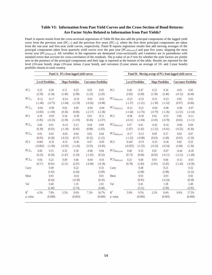
54
Table VI: Information from Past Yield Curves and the Cross-Section of Bond Returns: Are Factor Styles Related to Information from Past Yields?
Panel A reports results from the cross-sectional regressions of Table III that also add the principal components of the lagged yield curve from the previous year (PC t-1) and the previous five years (PC t-5), where the first three principal components are taken from the one-year and five-year yield curves, respectively. Panel B reports regression results that add moving averages of the principal components taken from quarterly yield curves over the past year (PCMA(1year)) and past five years, skipping the most recent year (PCMA(5year)). All variables in the regression are demeaned cross-sectionally and t-statistics are in parentheses with standard errors that account for cross-correlation of the residuals. The p-value of an F-test for whether the style factors are jointly zero in the presence of the principal components and their lags is reported at the bottom of the table. Results are reported for the level (10-year bond), slope (10-year minus 2-year bond), and curvature (5-year minus an average of 10- and 2-year bonds) portfolio returns in each country.
PC1 0.22 0.30 0.11 0.23 0.03 0.05 PC1 0.40 0.47 0.23 0.34 -0.01 0.02(2.59) (1.34) (1.40) (2.98) (1.23) (2.20) (2.82) (2.69) (1.58) (2.46) (-0.12) (0.44)
PC1t-1 -0.12 -0.17 -0.14 -0.19 -0.01 -0.02 PC1MA(1year) -0.23 -0.23 -0.21 -0.23 0.05 0.03(-1.40) (-0.75) (-1.64) (-2.19) (-0.26) (-0.98) (-1.37) (-1.21) (-1.30) (-1.52) (0.97) (0.66)
PC1t-5 -0.04 -0.09 0.02 0.00 -0.04 -0.04 PC1MA(5year) -0.12 -0.21 -0.04 -0.06 -0.06 -0.07(-0.82) (-1.69) (0.36) (0.06) (-2.17) (-2.58) (-1.64) (-2.76) (-0.79) (-1.26) (-2.51) (-3.14)
PC2 0.29 -0.05 0.34 -0.39 0.01 -0.11 PC2 -0.06 -0.30 0.62 -0.31 0.06 -0.11(1.85) (-0.23) (2.39) (-1.03) (0.26) (-2.07) (-0.21) (-1.04) (2.03) (-0.78) (0.65) (-1.11)
PC2t-1 0.06 0.01 -0.14 0.13 0.04 0.09 PC2MA(1year) 0.57 0.41 -0.45 -0.16 -0.06 0.04(0.39) (0.03) (-1.18) (0.45) (0.88) (1.83) (1.87) (1.42) (-1.32) (-0.41) (-0.52) (0.36)
PC2t-5 0.01 0.03 -0.05 0.04 0.02 0.04 PC2MA(5year) -0.17 -0.13 0.09 0.27 0.03 0.07(0.05) (0.28) (-0.55) (0.37) (0.52) (1.25) (-1.32) (-0.98) (0.63) (1.68) (0.65) (1.59)
PC3 -0.001 -0.32 -0.31 -0.46 0.47 -0.05 PC3 -0.447 -0.74 -0.23 -0.36 0.82 0.25(-0.002) (-1.06) (-0.92) (-1.43) (3.55) (-0.45) (-0.925) (-1.55) (-0.32) (-0.54) (3.68) (1.36)
PC3t-1 0.06 0.15 0.35 0.30 -0.08 0.04 PC3MA(1year) 0.40 0.33 0.01 -0.07 -0.44 -0.28(0.23) (0.58) (1.47) (1.29) (-1.05) (0.32) (0.73) (0.60) (0.02) (-0.11) (-2.21) (-1.49)
PC3t-5 0.04 0.22 0.49 0.46 -0.04 -0.01 PC3MA(5year) 0.25 0.60 0.93 0.84 -0.15 -0.03(0.17) (0.91) (2.21) (2.07) (-0.49) (-0.18) (0.78) (1.83) (2.91) (2.45) (-1.43) (-0.30)
Carry 0.49 0.22 0.35 Carry 0.48 0.21 0.32(1.92) (2.64) (3.09) (2.08) (2.98) (3.22)
Mom 0.03 -0.02 0.01 Mom 0.03 -0.01 0.02(0.42) (-0.38) (0.16) (0.95) (-0.24) (0.58)
Val 0.40 1.35 2.61 Val 0.41 1.58 2.40(2.40) (2.74) (4.48) (2.51) (2.90) (3.95)
R2 4.3% 7.8% 3.2% 9.0% 7.3% 16.7% R2 5.9% 9.5% 3.2% 9.4% 9.6% 17.5%p -value (0.089) (0.003) (0.000) p -value (0.000) (0.003) (0.000)
Curvature Portfolios
Panel A: PCs from lagged yield curves Panel B: Moving averge of PCs from lagged yield curves
Level Portfolios Slope PortfoliosLevel Portfolios Slope Portfolios Curvature Portfolios

55
Table VII: Unspanned Macroeconomic Factors Across Countries
The table reports results from the cross-sectional regressions of Table III that also add two macroeconomic variables: growth in industrial production and inflation for each country. The regressions test whether the unspanned factors of growth and inflation are priced in the cross-section of government bond excess returns in the presence of the first three principal components from the term structure of yields in each country. In addition, we add the style characteristics of carry, value, and momentum as additional unspanned factors and test whether they are spanned by the principal components and the macro variables and vice versa. All variables in the regression are demeaned cross-sectionally and t-statistics are in parentheses with standard errors that account for cross-correlation of the residuals. The p-values of nested F-tests for each successive model are reported at the bottom of the table. Panel A reports results for the level (10-year bond), Panel B for the slope (10-year minus 2-year bond), and Panel C for the curvature (5-year minus an average of 10- and 2-year bonds) of the yield curve in each country.
(1) (2) (3) (1) (2) (3) (1) (2) (3)
Growth -0.010 -0.050 -0.100 0.010 0.004 0.067 -0.032 -0.033 -0.014(-0.14) (-0.75) (-1.48) (0.18) (0.08) (1.18) (-1.61) (-1.60) (-0.62)
Inflation -0.035 -0.260 -0.071 0.018 -0.019 -0.010 0.022 -0.004 0.068(-0.40) (-2.74) (-1.32) (0.24) (-0.20) (-0.11) (0.77) (-0.16) (2.54)
PC1 0.140 0.083 0.024 0.013 0.002 -0.017(3.82) (2.06) (0.69) (0.38) (0.17) (-1.69)
PC2 0.244 -0.012 0.190 -0.055 0.046 -0.059(2.34) (-0.07) (1.75) (-0.25) (1.11) (-1.30)
PC3 -0.058 -0.245 0.079 0.021 0.416 -0.071(-0.27) (-1.07) (0.30) (0.08) (2.99) (-0.57)
Carry 0.367 0.279 0.313(1.94) (5.48) (3.04)
Mom -0.021 -0.038 -0.025(-1.02) (-1.58) (-0.62)
Val 0.357 0.645 2.710(2.35) (1.41) (3.87)
R2 0.04% 4.32% 6.57% 0.01% 0.82% 10.67% 0.58% 6.69% 17.30%p -value of nested F -test (0.000) (0.000) (0.065) (0.000) (0.000) (0.000)
vs (1) vs (2) vs (1) vs (2) vs (1) vs (2)
Panel A: Level Panel B: Slope Panel C: Curvature

56
Table VIII: Unspanned Cochrane-Piazzesi Factors Across Countries
The table reports results from time-series regressions of the 10-year government bond in each country on the single factor from Cochrane and Piazzesi (2005). The Cochrane and Piazzesi (2005) factor is formed from a panel regression of the average returns across 2 to 10-year maturity bonds in each country on the 1, 3, and 5-year forward rates in each country, estimated across all countries over the full sample period. The coefficients from this regression (detailed in Appendix B and exhibiting the familiar tent-shaped pattern) are used to form the single factor. Subsequent columns below add the first three principal components from the term structure of yields in each country, and the style characteristics of value, momentum, and carry. The sample is from Wright (2011) and covers the period 1971 to 2016.
CP 1.53 1.82 0.90 1.69 1.27 0.71 0.52CP#T-Sta (5.22) (2.09) (1.04) (1.83) (1.29) (1.37) (0.48)PC1 -0.08 -0.16 -0.09 0.03 -0.14PC1#T-Stat (-0.55) (-1.11) (-0.62) (0.20) (-0.73)PC2 -0.26 0.71 0.27 -0.38 1.24PC2#T-Stat (-0.23) (0.62) (0.22) (-0.34) (1.03)PC3 -0.45 0.53 -0.05 -0.30 1.01PC3#T-Stat (-0.29) (0.32) (-0.03) (-0.19) (0.58)Val 1.30 0.95 1.36Val#T-Stat (2.70) (2.05) (2.49)Mom -0.17 -0.16 -0.19Mom#T-Stat (-2.30) (-2.38) (-2.68)Carry 0.95 1.34 0.37Carry#T-Stat (1.25) (1.91) (0.41)Intercept -1.98% -1.39% -1.63% -0.88% -1.63% -1.60% -0.96%Intercept (-1.48) (-0.67) (-0.78) (-0.42) (-0.78) (-1.03) (-0.45)
R 2 12.25% 12.50% 16.21% 16.51% 13.03% 19.23% 20.18%
Dependent variable = 10-year bond excess return, rx t+1(10)

57
Table IX: Out of Sample Tests Using Tradeable Bond Portfolios The table reports summary statistics on the performance of the style strategies as well as strategies based on the first three principal components of the yield curve using tradeable bond portfolios and live returns for country selection based on level, slope, and butterfly returns. In each country we form a “country asset” as an equal duration-weighted portfolio across 1y-5y, 5y-10y and 10y-30y country-maturity portfolios. For each style we form a duration-neutral long-short portfolio across country assets. In each country we form a “slope asset” that is long the 10y-30y country-maturity portfolio and short the 1y-5y country-maturity portfolio, in a duration neutral manner. For each style we form a “slope neutral” long-short portfolio across country slope assets. In each country we form a “butterfly asset” that is long the 5y-10y country-maturity portfolio and short the 1y-5y and 10y-30y country-maturity portfolios. We construct the butterflies such that the total has duration of zero and the 1y-5y country-maturity portfolio has the same duration as the 10y-30y country-maturity portfolio. For each style and each selection strategy (country level, slope, butterfly), we first rank the universe of securities by the raw measure of a given style. We then standardize the ranks by subtracting the mean rank from each rank and dividing by the standard deviation of ranks to convert them into a set of standardized weights. We also form portfolios based on PC1 through PC3 using the JPM live bond portfolios, where we compute the PCs on the 1-5, 5-10, and 10-30 yield data and sign the PCs based on the coefficient estimates from Tables III and IV, which uses the entire sample to estimate the regression coefficients. We also combine our style long-short strategies to produce a multi-style composite portfolio that diversifies across value, momentum, and carry and combine our PC-based strategies as well across all three PC weightings (“combo”). We report results for level, slope, and butterfly portfolio returns in Panels A, B, and C, respectively, and we report in Panel D results that diversify across level, slope, and butterfly returns (“multi-dimension”).
Value Momentum Carry Multi-style PC1 PC2 PC3 Combo
Average 3.82% 2.11% 3.35% 3.10% 2.94% 0.69% -0.63% 1.00%Stdev 5.9% 6.2% 5.7% 3.1% 5.7% 4.4% 3.8% 3.4%t -stat 3.0 1.6 2.7 4.6 2.4 0.7 -0.8 1.4Sharpe 0.65 0.34 0.58 1.01 0.52 0.16 -0.17 0.30Correl to market 0.13 0.09 0.10 0.20 0.19 0.15 0.03 0.18Alpha to market 3.02% 1.57% 2.79% 2.46% 1.87% 0.01% -0.76% 0.37%t -stat 2.3 1.1 2.1 3.6 1.5 0.0 -0.9 0.5Info ratio 0.52 0.26 0.49 0.82 0.33 0.00 -0.20 0.11Skewness -0.07 0.52 -0.66 0.25 0.30 -0.32 -0.49 -0.79Kurtosis 4.4 5.1 7.6 5.9 3.6 3.4 3.5 5.1Autocorrelation 0.05 0.05 0.05 0.13 0.02 0.13 -0.07 -0.01
Beta to PC1 0.94 -0.32 0.29 0.57 Beta to Carry -0.06 0.77 0.27 0.40(54.60) (-5.14) (6.84) (12.97) (-2.86) (14.04) (3.56) (9.88)
Beta to PC2 0.06 -0.08 0.60 0.36 Beta to Mom -0.03 0.12 -0.05 0.01(3.10) (-1.28) (13.35) (7.69) (-1.75) (2.38) (-0.70) (0.38)
Beta to PC3 0.06 -0.11 0.05 0.00 Beta to Val 0.98 0.00 0.07 0.58(3.25) (-1.72) (1.24) (-0.06) (48.18) (-0.02) (0.90) (14.90)
Alpha to PCs 1.67% 5.02% 3.47% 6.58% Alpha to Styles -0.75% -3.33% -3.49% -3.18%(2.94) (2.46) (2.46) (4.56) (-1.24) (-2.12) (-1.62) (-2.75)
Value Momentum Carry Multi-style PC1 PC2 PC3 Combo
Average 0.77% 0.48% 1.47% 0.91% -0.57% 0.19% -0.75% -0.37%Stdev 1.8% 1.9% 2.1% 1.2% 2.3% 1.7% 1.7% 1.0%t -stat 2.0 1.2 3.2 3.4 -1.1 0.5 -2.0 -1.7Sharpe 0.43 0.26 0.69 0.73 -0.25 0.11 -0.44 -0.36Correl to market -0.04 0.18 0.14 0.15 -0.16 -0.15 0.16 -0.11Alpha to market 0.85% 0.14% 1.17% 0.72% -0.20% 0.44% -1.02% -0.26%t -stat 2.1 0.3 2.5 2.6 -0.4 1.2 -2.7 -1.1Info ratio 0.47 0.08 0.56 0.59 -0.09 0.26 -0.61 -0.25Skewness 1.92 0.53 1.25 3.82 -1.58 0.64 0.73 -1.56Kurtosis 13.3 3.8 8.6 30.3 10.3 3.7 7.2 10.1Autocorrelation -0.02 -0.05 -0.04 -0.19 -0.01 0.04 -0.07 0.04
Beta to PC1 -0.59 -0.15 -0.54 -0.67 Beta to Carry -0.53 -0.35 0.14 -0.50(-14.70) (-2.57) (-10.89) (-13.86) (-11.24) (-7.05) (2.15) (-9.03)
Beta to PC2 0.61 -0.33 -0.29 -0.03 Beta to Mom -0.06 -0.14 -0.02 -0.14(15.11) (-5.38) (-5.71) (-0.69) (-1.33) (-2.85) (-0.36) (-2.46)
Beta to PC3 -0.07 -0.06 -0.03 -0.08 Beta to Val -0.45 0.55 -0.15 -0.12(-1.85) (-0.93) (-0.53) (-1.63) (-10.21) (11.65) (-2.38) (-2.21)
Alpha to PCs 1.83% 2.29% 5.80% 5.35% Alpha to Styles 3.27% 1.57% -4.72% 0.71%(1.34) (1.11) (3.42) (3.23) (2.13) (0.96) (-2.14) (0.39)
Panel A: Level returns
Panel B: Slope returns

58
Value Momentum Carry Multi-style PC1 PC2 PC3 Combo
Average 0.41% 0.02% 0.72% 0.38% -0.23% 0.18% 0.35% 0.10%Stdev 0.5% 0.6% 0.6% 0.3% 0.6% 0.6% 0.5% 0.4%t -stat 3.5 0.2 5.3 5.3 -1.6 1.4 3.0 1.3Sharpe 0.77 0.04 1.15 1.16 -0.36 0.30 0.65 0.28Correl to market 0.06 0.06 0.10 0.13 0.02 0.40 -0.04 0.21Alpha to market 0.38% -0.01% 0.66% 0.34% -0.24% -0.06% 0.38% 0.02%t -stat 3.1 -0.1 4.6 4.6 -1.6 -0.5 3.0 0.3Info ratio 0.71 -0.02 1.05 1.04 -0.37 -0.12 0.69 0.07Skewness -0.45 0.31 1.12 1.34 -1.07 0.63 0.31 0.22Kurtosis 6.4 4.4 8.9 10.3 6.8 4.2 4.1 13.8Autocorrelation -0.19 -0.12 -0.10 -0.08 -0.18 -0.16 -0.03 -0.31
Beta to PC1 0.39 -0.56 -0.55 -0.49 Beta to Carry -0.37 -0.18 0.18 -0.23(9.23) (-10.95) (-10.17) (-9.04) (-7.25) (-2.68) (3.29) (-4.64)
Beta to PC2 0.17 0.07 -0.04 0.11 Beta to Mom -0.26 0.22 -0.01 -0.04(3.90) (1.43) (-0.74) (2.03) (-4.53) (2.83) (-0.18) (-0.66)
Beta to PC3 0.58 -0.17 0.14 0.29 Beta to Val 0.29 0.22 0.64 0.62(13.70) (-3.31) (2.56) (5.35) (5.56) (3.04) (11.16) (11.95)
Alpha to PCs 4.79% -0.76% 8.74% 7.63% Alpha to Styles -1.50% 3.39% -0.46% 0.76%(3.22) (-0.42) (4.63) (3.98) (-0.88) (1.46) (-0.25) (0.46)
Value Momentum Carry Multi-style PC1 PC2 PC3 Combo
Average 6.14% 2.11% 8.07% 9.67% -0.29% 1.90% 0.13% 0.73%Stdev 6.5% 6.2% 7.4% 7.3% 5.3% 5.4% 6.9% 5.7%t -stat 4.4 1.6 5.0 6.1 -0.2 1.6 0.1 0.6Sharpe 0.95 0.34 1.09 1.32 -0.05 0.35 0.02 0.13Correl to market 0.08 0.17 0.15 0.22 0.03 0.25 0.07 0.17Alpha to market 5.65% 1.03% 6.95% 8.05% -0.45% 0.52% -0.37% -0.24%t -stat 3.8 0.7 4.2 5.0 -0.4 0.4 -0.2 -0.2Info ratio 0.87 0.17 0.95 1.13 -0.08 0.10 -0.05 -0.04
Skewness 1.34 0.03 1.62 2.71 -0.48 0.67 0.35 -1.19Kurtosis 7.3 3.5 14.2 21.7 5.5 4.9 11.1 13.9Autocorrelation -0.05 0.01 0.03 0.02 -0.10 -0.17 -0.06 -0.19
Beta to PC1 0.21 -0.27 -0.32 -0.22 Beta to Carry -0.34 -0.05 0.25 -0.16(3.89) (-4.57) (-5.50) (-3.69) (-5.68) (-0.76) (3.88) (-2.75)
Beta to PC2 0.39 -0.02 0.08 0.22 Beta to Mom -0.13 0.08 -0.21 -0.15(7.11) (-0.28) (1.42) (3.76) (-2.07) (1.33) (-3.24) (-2.52)
Beta to PC3 0.23 -0.18 0.24 0.17 Beta to Val 0.29 0.45 0.16 0.45(4.33) (-3.08) (4.19) (2.87) (4.79) (7.20) (2.44) (7.65)
Alpha to PCs 8.20% 3.35% 10.38% 12.29% Alpha to Styles 0.84% -0.53% -3.26% -0.77%(4.38) (1.62) (5.14) (5.95) (0.40) (-0.25) (-1.49) (-0.38)
Panel C: Butterfly returns
Panel D: Multi-dimension returns

59
Table X: Correlation Across Styles within Yield Curve Dimension The table reports the correlations of the style strategies – value, momentum, and carry – within each asset category. Panel A reports the correlations within the country level portfolios, Panel B reports correlations of style returns for country slope portfolios, Panel C reports correlations for the butterfly portfolios across countries and Panel D reports correlations of style strategies that combine the multiple dimensions of the yield curve across the level, slope, and butterfly portfolios (multi-dimension). Panel E reports results from regressions of each style strategy’s returns on the other style strategy returns within each asset category.
Carry Momentum Value Carry Momentum ValueCarry 1.00 1.00Momentum -0.45 1.00 0.36 1.00Value 0.55 -0.36 1.00 0.07 -0.13 1.00
Carry Momentum Value Carry Momentum ValueCarry 1.00 1.00Momentum 0.45 1.00 0.22 1.00Value -0.16 -0.51 1.00 0.23 -0.27 1.00
Value Momentum Carry Alpha R 2 Optimal weightLevelValue -0.14 0.49 0.34% 32.2% 29.7%
(-2.46) (8.38) (2.22)Momentum -0.17 -0.36 0.55% 21.9% 39.2%
(-2.46) (-5.31) (3.33)Carry 0.45 -0.28 0.32% 37.6% 31.1%
(8.38) (-5.31) (2.18)SlopeValue -0.17 0.13 0.32% 3.1% 39.1%
(-2.60) (1.95) (1.74)Momentum -0.15 0.37 0.05% 15.5% 6.9%
(-2.60) (6.41) (0.30)Carry 0.12 0.38 0.46% 14.5% 53.9%
(1.95) (6.41) (2.67)ButterflyValue -0.54 0.08 0.58% 26.2% 46.8%
(-8.93) (1.28) (3.49)Momentum -0.45 0.37 -0.04% 39.2% 0.0%
(-8.93) (7.44) (-0.26)Carry 0.08 0.49 0.89% 20.3% 53.2%
(1.28) (7.44) (5.27)Multi-DimensionValue -0.34 0.30 0.61% 16.3% 43.9%
(-5.76) (5.12) (3.50)Momentum -0.34 0.30 0.29% 15.9% 21.2%
(-5.76) (4.98) (1.60)Carry 0.31 0.30 0.57% 13.8% 34.9%
(5.12) (4.98) (3.22)
Panel E: Factor Portfolio Regressions on Other Factors
Panel B: SlopePanel A: Level
Panel C: Butterfly/Curvature Panel D: Multi-Dimension

60
Table XI: Correlation Across Yield Curve Dimensions within Style
The table reports correlations across the asset categories for a given style. Panel A reports the correlations for value strategies across level, slope, and butterfly portfolios, Panel B reports the correlation of momentum strategies across the asset categories, and Panel C reports correlations among carry strategies. Panel D reports correlations of multi-style strategies – diversified across value, momentum, and carry – in each of the asset categories.
Level value Slope value Butterfly value Level momentum Slope momentum Butterfly momentumLevel value 1.00 Level momentum 1.00Slope value 0.16 1.00 Slope momentum -0.08 1.00Butterfly value 0.13 0.09 1.00 Butterfly momentum -0.01 0.32 1.00Multi-dimension value 0.67 0.64 0.63 Multi-dimension momentum 0.49 0.67 0.70
Level carry Slope carry Butterfly carry Level multi-style Slope multi-style Butterfly multi-styleLevel carry 1.00 Level multi-style 1.00Slope carry 0.58 1.00 Slope multi-style 0.44 1.00Butterfly carry 0.07 0.32 1.00 Butterfly multi-style 0.10 0.36 1.00Multi-dimension carry 0.74 0.85 0.63 Multi-dimension, multi-style 0.71 0.82 0.67
Panel A: Value Correlations Panel B: Momentum Correlations
Panel C: Carry Correlations Panel D: Multi-Style Correlations

61
Table XII: Regression on Style Factors from Other Asset Classes
The table reports regression results of our bond style returns for level, slope, and butterfly portfolios on style returns from other asset classes: equity index futures, currencies, and commodities, as well as the global bond market portfolio, GBI in excess of the T-bill rate (Mkt – rf). The value and momentum strategies in other asset classes are those from Asness, Moskowitz, and Pedersen (2013), and the carry strategies are from Koijen, Moskowitz, Pedersen, and Vrugt (2016). All series, including our bond factors, are scaled to 10% annualized volatility using the full sample estimate of each strategy’s standard deviation. Panel A reports results for value strategies among country portfolios based on level, slope, butterfly, and their combination (multi-dimension), and Panels B and C report results for momentum and carry, respectively. Panel D reports the diversified multi-style returns for each government bond strategy regressed on the multi-style returns for equities, currencies, and commodities (plus the global bond market). The R2 reported in the last column is the marginal R2 relative to a regression with the bond market only.
EQ value FX value Com value Mkt-rf Alpha Marginal R 2
Level value 0.28 0.23 -0.01 0.46 0.33% 13.0%(4.69) (3.96) (-0.09) (2.38) (1.87)
Slope value -0.03 0.05 -0.02 -0.15 0.38% 0.3%(-0.42) (0.74) (-0.31) (-0.73) (2.01)
Butterfly value 0.06 -0.09 0.00 0.20 0.61% 1.1%(0.95) (-1.34) (0.07) (0.97) (3.19)
Multi-dimension value 0.16 0.10 -0.01 0.26 0.68% 3.5%(2.55) (1.61) (-0.17) (1.28) (3.62)
EQ mom FX mom Com mom Mkt-rf Alpha Marginal R 2
Level mom 0.12 0.21 0.18 0.28 0.10% 10.9%(1.91) (3.34) (3.00) (1.43) (0.56)
Slope mom 0.00 0.06 0.04 0.59 0.04% 0.5%(-0.06) (0.88) (0.63) (2.85) (0.21)
Butterfly mom 0.01 -0.08 0.03 0.19 -0.01% 0.8%(0.13) (-1.29) (0.48) (0.93) (-0.04)
Multi-dimension mom 0.07 0.10 0.13 0.57 0.07% 3.8%(1.04) (1.51) (2.18) (2.81) (0.39)
EQ carry FX carry Com carry Mkt-rf Alpha Marginal R 2
Level carry 0.15 0.30 -0.06 0.30 0.29% 12.5%(2.57) (5.11) (-0.97) (1.48) (1.56) (0.00)
Slope carry 0.11 0.08 -0.05 0.40 0.44% 2.2%(1.71) (1.34) (-0.79) (1.90) (2.31) (0.13)
Butterfly carry -0.02 -0.01 0.11 0.38 0.82% 1.2%(-0.35) (-0.14) (1.69) (1.76) (4.25) (0.40)
Multi-dimension carry 0.11 0.17 0.00 0.48 0.70% 4.3%(1.73) (2.75) (-0.00) (2.32) (3.69) (0.01)
EQ all FX all Com all Mkt-rf Alpha Marginal R 2
Level multi-style 0.15 0.27 0.12 0.70 0.39% 11.8%(2.58) (4.61) (2.09) (3.58) (2.14) (0.00)
Slope multi-style 0.04 0.08 0.00 0.49 0.42% 0.8%(0.60) (1.26) (0.06) (2.32) (2.14) (0.55)
Butterfly multi-style 0.05 -0.12 0.07 0.41 0.91% 2.2%(0.84) (-1.92) (1.14) (1.97) (4.68) (0.14)
Multi-dimension, multi-style 0.11 0.11 0.09 0.73 0.78% 3.3%(1.80) (1.71) (1.47) (3.57) (4.13) (0.03)
Panel A: Value
Panel B: Momentum
Panel C: Carry
Panel D: Multi-Style

62
Table XIII: Regression on Other Risk Factors
The table reports regression results for level, slope, and butterfly strategies that diversify across the three styles – value, momentum, and carry, denoted “multi-style” – as well as value, momentum, and carry strategies that diversify across yield curve portfolios – level, slope, and butterfly, denoted “multi-dimension” – and a strategy that diversifies across both styles and yield curve dimensions. The independent variables are a host of global bond, equity, volatility, and liquidity factors. We use a measure of equity volatility (EQVOL) and bond volatility (FIVOL) designed to approximate the returns to selling volatility. EQVOL are the returns to selling front-month at-the-money S&P500 straddles sized to a constant notional amount, delta-hedged daily, and held until expiration and FIVOL are the returns to selling front-month at-the-money US 10-year Treasury futures straddles sized to a constant notional amount, delta-hedge daily, and held until expiration. We also include the GBI, which is USD hedged excess returns of the JP Morgan Government Bond Index, the Barclays Global High-Yield Index (below investment grade corporate debt) in excess of duration-matched Treasuries (HY), and the excess returns on the S&P 500 index (SPX). We also include the on-the-run versus off-the-run Treasury spread (OTR), which is the difference in returns between the most recent 10-year off-the-run US Treasury and the on-the-run 10-year Treasury matched in duration and financed by the 3-month Treasury bill rate.
EQVOL FIVOL GBI HY OTR SPX Alpha R 2
Level multi-style -0.02 0.69 0.95 0.10 -1.41 0.10 0.58% 5.4%(-0.06) (0.60) (4.05) (1.14) (-0.58) (1.91) (2.87)
Slope multi-style 0.32 2.17 0.59 0.10 3.01 0.02 0.27% 4.6%(0.83) (1.84) (2.48) (1.08) (1.21) (0.32) (1.28)
Butterfly multi-style -0.05 0.33 0.87 0.33 -2.06 -0.07 0.81% 6.9%(-0.12) (0.29) (3.73) (3.79) (-0.85) (-1.30) (3.99)
Multi-dimension value 0.23 0.09 0.48 0.13 -3.02 0.07 0.63% 6.0%(0.63) (0.08) (2.08) (1.48) (-1.26) (1.38) (3.16)
Multi-dimension mom -0.05 1.11 0.56 0.01 -0.77 0.00 0.15% 0.5%(-0.14) (0.97) (2.42) (0.09) (-0.32) (0.09) (0.72)
Multi-dimension carry 0.06 1.60 0.91 0.28 3.03 -0.03 0.58% 8.2%(0.15) (1.41) (3.92) (3.28) (1.26) (-0.58) (2.88)
Multi-dimension, multi-style 0.12 1.46 1.10 0.24 -0.21 0.02 0.76% 7.8%(0.31) (1.28) (4.78) (2.79) (-0.09) (0.44) (3.79)

63
Appendix A
Table A1: More Information from Past Yield Curves on Bond Returns
The table reports results from the cross-sectional regressions of Table III that also add the principal components of the lagged yield curve from each of the previous k-years (PC t-k) over the last five years, where the first three principal components are taken from the one-year average of quarterly yield curves each year over the past five years. All variables in the regression are demeaned cross-sectionally and t-statistics are in parentheses with standard errors that account for cross-correlation of the residuals. The p-value of an F-test for whether the style factors are jointly zero in the presence of the principal components and their lags is reported at the bottom of the table. Results are reported for the level (10-year bond), slope (10-year minus 2-year bond), and curvature (5-year minus an average of 10- and 2-year bonds) portfolio returns in each country.
PC1 0.47 0.49 0.22 0.32 -0.03 0.00(3.19) (2.75) (1.35) (2.23) (-0.43) (0.07)
PC1t-1 -0.39 -0.33 -0.20 -0.19 0.10 0.08(-1.93) (-1.74) (-0.85) (-0.87) (1.06) (0.91)
PC1t-2 0.14 0.07 0.01 -0.01 -0.07 -0.07(0.94) (0.41) (0.04) (-0.09) (-1.10) (-1.18)
PC1t-3 -0.25 -0.21 0.01 -0.01 0.05 0.04(-1.51) (-1.32) (0.05) (-0.07) (0.86) (0.76)
PC1t-4 0.21 0.18 -0.11 -0.07 -0.04 -0.03(1.47) (1.29) (-1.07) (-0.73) (-0.82) (-0.70)
PC1t-5 -0.13 -0.17 0.05 0.00 -0.02 -0.03(-1.34) (-1.81) (0.69) (0.06) (-0.95) (-1.48)
PC2 -0.16 -0.38 0.72 -0.38 0.11 -0.05(-0.52) (-1.21) (1.92) (-0.92) (0.97) (-0.49)
PC2t-1 0.71 0.58 -0.65 -0.37 -0.17 -0.08(1.92) (1.63) (-1.27) (-0.78) (-1.10) (-0.58)
PC2t-2 -0.12 -0.18 0.13 0.37 0.09 0.13(-0.57) (-0.81) (0.41) (0.99) (1.10) (1.63)
PC2t-3 0.03 0.11 0.11 0.07 0.03 0.01(0.14) (0.58) (0.41) (0.26) (0.37) (0.17)
PC2t-4 -0.36 -0.32 0.10 0.15 -0.02 -0.02(-1.90) (-1.72) (0.42) (0.69) (-0.34) (-0.26)
PC2t-5 0.29 0.26 -0.18 -0.11 0.00 0.03(1.80) (1.61) (-1.15) (-0.68) (-0.02) (0.50)
PC3 -0.71 -0.98 -0.05 -0.22 0.93 0.36(-1.50) (-2.10) (-0.06) (-0.28) (3.63) (1.78)
PC3t-1 0.95 0.89 -0.43 -0.46 -0.62 -0.45(1.56) (1.51) (-0.46) (-0.51) (-2.24) (-1.81)
PC3t-2 -0.47 -0.46 0.64 0.46 0.14 0.13(-1.09) (-1.06) (1.38) (1.09) (0.89) (0.82)
PC3t-3 0.70 0.87 -0.06 -0.02 -0.18 -0.08(1.59) (1.96) (-0.13) (-0.05) (-1.25) (-0.61)
PC3t-4 -0.23 -0.21 0.17 0.16 -0.08 -0.05(-0.58) (-0.56) (0.48) (0.47) (-0.68) (-0.46)
PC3t-5 0.05 0.18 0.41 0.45 0.06 0.05(0.16) (0.58) (1.29) (1.44) (0.64) (0.57)
Carry 0.47 0.22 0.34(1.95) (2.74) (3.21)
Mom 0.02 -0.04 0.01(0.57) (-0.87) (0.32)
Val 0.40 1.63 2.23(2.47) (3.04) (3.82)
R2 7.4% 10.7% 4.4% 10.5% 10.9% 18.5%p -value (0.001) (0.015) (0.000)
Level Portfolios Slope Portfolios Curvature Portfolios

64
Appendix B
Table B1: Cochrane-Piazzesi Regressions by Country
The table reports regression coefficient estimates from Cochrane and Piazzesi (2005) type regressions for each country that regress the average of 2 to 10-year government bonds in each country on the one, three, and five-year forward rates in each country. Country bond returns come from Wright (2011), which are smoothed data using a three factor model and hence only three forward rates can be used as regressors otherwise the regression is overidentified, for seven coutnries: AU, BD, CN, JP, SD, UK, and the US covering the period 1971 to 2016 that varies by country (see the table in footnote 5). In addition, results are reported for US-only government bond data from Fama and Bliss (1987) that covers one to five-year maturities and the period 1964 to 2013, labeled US (FB). Finally, results are reported for a panel regression of all countries bond returns (averaged across 2 to 10-year maturities) on the forward rates, including country fixed effects.
f (1) f (3) f (5) Intercept R 2 T
AU -1.69 2.71 -0.35 -2.13% 10.99% 113AU (-1.87) (1.49) (-0.16) (-0.60)BD -1.25 -0.14 1.67 -0.66% 8.21% 169BD (-1.15) (-0.06) (0.90) (-0.26)CN -2.05 1.93 0.38 0.13% 12.92% 117CN (-2.39) (0.93) (0.21) (0.06)JP -3.27 3.29 0.60 -0.75% 23.98% 121JP (-1.88) (0.70) (0.19) (-0.60)SD -2.30 3.29 -0.15 -1.47% 15.33% 90SD (-1.69) (0.99) (-0.06) (-0.52)UK -2.20 2.69 -0.23 -0.37% 11.46% 145UK (-3.00) (2.16) (-0.19) (-0.14)US -2.76 1.83 1.66 -4.69% 18.13% 174US (-2.24) (0.65) (0.74) (-1.21)
US (FB) -4.21 7.86 -3.50 -0.05% 27.77% 169US (-5.43) (4.90) (-3.04) (-0.02)
Panel -2.09 1.68 0.86 12.48% 929(-4.52) (1.62) (1.01)
19�𝑟𝑥(𝑛)
𝑡+1
10
𝑛=2
= 𝛽0 + 𝛽1𝑓(1)𝑡 + 𝛽2𝑓(3)
𝑡 + 𝛽3𝑓(5)𝑡 + 𝜀�̅�+1

65
Figure B1: Forward Rate Coefficients from Cochrane-Piazzesi Regressions by Country and Maturity. Plotted are the regression coefficient estimates from Cochrane and Piazzesi (2005) type regressions for each country that regress each bond from 2 to 10-year maturities in each country on the one, three, and five-year forward rates in each country. Country bond returns come from Wright (2011), which are smoothed data using a three factor model and hence only three forward rates can be used as regressors otherwise the regression is overidentified, for seven coutnries: AU, BD, CN, JP, SD, UK, and the US covering the period 1971 to 2016 that varies by country (see the table in footnote 5). In addition, results are reported for US-only government bond data from Fama and Bliss (1978) that covers one to five-year maturities and the period 1964 to 2013, labeled US (FB), as well as live U.S. returns from the JP Morgan tradeable bond data beginning in 1993 and the U.S. data from Wright (2011) and from Fama-Bliss post-1993.
-3.0
-2.0
-1.0
0.0
1.0
2.0
3.0
4.0
F_01 F_03 F_05
AU
2
3
4
5
6
7
8
9
10
-3.0
-2.0
-1.0
0.0
1.0
2.0
3.0
4.0
5.0
F_01 F_03 F_05
BD
2
3
4
5
6
7
8
9
10
-4.0
-3.0
-2.0
-1.0
0.0
1.0
2.0
3.0
F_01 F_03 F_05
CN
2
3
4
5
6
7
8
9
10-5.0
-4.0
-3.0
-2.0
-1.0
0.0
1.0
2.0
3.0
4.0
5.0
F_01 F_03 F_05
JP
2
3
4
5
6
7
8
9
10
-5.0
-4.0
-3.0
-2.0
-1.0
0.0
1.0
2.0
3.0
4.0
5.0
F_01 F_03 F_05
SD
2
3
4
5
6
7
8
9
10
-4.0
-3.0
-2.0
-1.0
0.0
1.0
2.0
3.0
4.0
F_01 F_03 F_05
UK
2
3
4
5
6
7
8
9
10

66
-5.0
-4.0
-3.0
-2.0
-1.0
0.0
1.0
2.0
3.0
4.0
5.0
F_01 F_03 F_05
US (Wright Data, 1971-)
2
3
4
5
6
7
8
9
10
-10.0
-5.0
0.0
5.0
10.0
15.0
F_01 F_03 F_05
US (Fama-Bliss, 1964-)
2
3
4
5
6
7
8
9
10-6.0
-4.0
-2.0
0.0
2.0
4.0
6.0
8.0
F_01 F_03 F_05
US (Live Returns, 1993-)
2
3
4
5
6
7
8
9
10
-3.0
-2.0
-1.0
0.0
1.0
2.0
3.0
4.0
5.0
F_01 F_03 F_05
US (Fama-Bliss, 1993-)
2
3
4
5
6
7
8
9
10-6.0
-4.0
-2.0
0.0
2.0
4.0
6.0
8.0
F_01 F_03 F_05
US (Wright Data, 1993-)
2
3
4
5
6
7
8
9
10

67
Figure B2: Forward Rate Coefficients from Cochrane-Piazzesi Regressions by Country. Plotted are the regression coefficient estimates from Cochrane and Piazzesi (2005) type regressions for each country that regresses the average of 2 to 10-year government bonds in each country on the one, three, and five-year forward rates in each country. Country bond returns come from Wright (2011), which are smoothed data using a three factor model and hence only three forward rates can be used as regressors otherwise the regression is overidentified, for seven coutnries: AU, BD, CN, JP, SD, UK, and the US covering the period 1971 to 2016 that varies by country (see the table in footnote 5). In addition, coefficients are plotted for US-only government bond data from Fama and Bliss (1987) that covers one to five-year maturities and the period 1964 to 2013, labeled US (FB). Finally, coefficients are plotted from a panel regression of all countries’ bond returns (averaged across 2 to 10-year maturities) on the forward rates, including country fixed effects. A correlation matrix of the resulting Cochrane-Piazzesi factors across countries is reported at the bottom of the figure.
-6.0
-4.0
-2.0
0.0
2.0
4.0
6.0
8.0
10.0
Forward (1 year) Forward (3 year) Forward (5 year)
AU BD CN JP SD UK US US (FB) Panel
AU BD CN JP SD UK US1.00 0.53 0.75 0.66 0.71 0.71 0.68
1.00 0.60 0.63 0.86 0.39 0.321.00 0.54 0.76 0.70 0.70
1.00 0.67 0.46 0.231.00 0.59 0.41
1.00 0.531.00
Correlation of Cochrane-Piazzesi Factor Across Countries

68
Disclosure: AQR Capital is a global investment manager who may or may not use the ideas in this paper. The views and opinions expressed are those of the authors and do not necessarily reflect the views of AQR Capital Management.


