Waveform modeling of historical seismograms of the 1930 Irpinia earthquake provides insight on “blind” faulting in Southern Apennines (Italy

Waveform modeling of historical seismograms of the 1930 Irpinia

earthquake provides insight on ‘‘blind’’ faulting in Southern

Apennines (Italy)

N. A. Pino,1 B. Palombo,2 G. Ventura,3 B. Perniola,4 and G. Ferrari5

Received 7 June 2007; revised 27 September 2007; accepted 22 January 2008; published 6 May 2008.

[1] The Southern Apennines chain is related to the west-dipping subduction of theApulian lithosphere. The strongest seismic events mostly occurred in correspondence ofthe chain axis along normal NW–SE striking faults parallel to the chain axis. Thesestructures are related to mantle wedge upwelling beneath the chain. In the foreland,faulting develops along E–W strike-slip to oblique-slip faults related to the roll-backof the foreland. Similarly to other historical events in Southern Apennines, theI0 = XI (MCS intensity scale) 23 July 1930 earthquake occurred between the chainaxis and the thrust front without surface faulting. This event produced more than1400 casualties and extensive damage elongated approximately E-W. The analysis of thehistorical waveforms provides the chance to study the fault geometry of this ‘‘anomalous’’event and allow us to clarify its geodynamic significance. Our results indicate thatthe MS = 6.6 1930 event nucleated at 14.6 ± 3.06 km depth and ruptured a north dipping,N100�E striking plane with an oblique motion. The fault propagated along the fault strike32 km to the east at about 2 km/s. The eastern fault tip is located in proximity of theVulture volcano. The 1930 hypocenter, similarly to the 1990 (MW = 5.8) SouthernApennines event, is within the Mesozoic carbonates of the Apulian foredeep and therupture developed along a ‘‘blind’’ fault. The 1930 fault kinematics significantly differsfrom that typical of large Southern Apennines earthquakes, which occur in a distinctseismotectonic domain on late Pleistocene to Holocene outcropping faults.These results stress the role played by pre-existing, ‘‘blind’’ faults in the Apenninessubduction setting.

Citation: Pino, N. A., B. Palombo, G. Ventura, B. Perniola, and G. Ferrari (2008), Waveform modeling of historical seismograms of

the 1930 Irpinia earthquake provides insight on ‘‘blind’’ faulting in Southern Apennines (Italy), J. Geophys. Res., 113, B05303,

doi:10.1029/2007JB005211.

1. Introduction

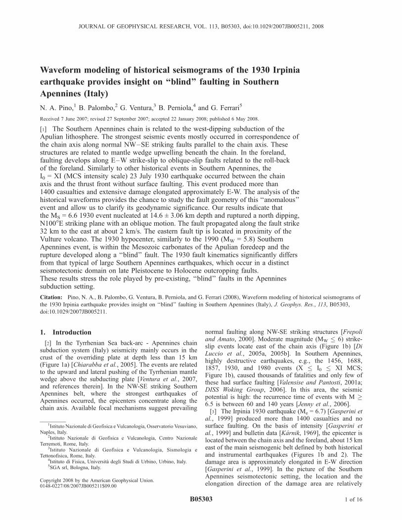
[2] In the Tyrrhenian Sea back-arc - Apennines chainsubduction system (Italy) seismicity mainly occurs in thecrust of the overriding plate at depth less than 15 km(Figure 1a) [Chiarabba et al., 2005]. The events are relatedto the upward and lateral pushing of the Tyrrhenian mantlewedge above the subducting plate [Ventura et al., 2007,and references therein]. In the NW-SE striking SouthernApennines belt, where the strongest earthquakes ofApennines occurred, the epicenters concentrate along thechain axis. Available focal mechanisms suggest prevailing

normal faulting along NW-SE striking structures [Frepoliand Amato, 2000]. Moderate magnitude (MW � 6) strike-slip events locate east of the chain axis (Figure 1b) [DiLuccio et al., 2005a, 2005b]. In Southern Apennines,highly destructive earthquakes, e.g., the 1456, 1688,1857, 1930, and 1980 events (X � I0 � XI MCS;Figure 1b), caused thousands of fatalities and only few ofthese had surface faulting [Valensise and Pantosti, 2001a;DISS Woking Group, 2006]. In this area, the seismicpotential is high: the recurrence time of events with M �6.5 is between 60 and 140 years [Jenny et al., 2006].[3] The Irpinia 1930 earthquake (Me = 6.7) [Gasperini et

al., 1999] produced more than 1400 casualties and nosurface faulting. On the basis of intensity [Gasperini etal., 1999] and bulletin data [Karnik, 1969], the epicenter islocated between the chain axis and the foreland, about 15 kmeast of the main seismogenic belt defined by both historicaland instrumental earthquakes (Figures 1b and 2). Thedamage area is approximately elongated in E-W direction[Gasperini et al., 1999]. In the picture of the SouthernApennines seismotectonic setting, the location and theelongation direction of the damage area are relatively

JOURNAL OF GEOPHYSICAL RESEARCH, VOL. 113, B05303, doi:10.1029/2007JB005211, 2008

1Istituto Nazionale di Geofisica e Vulcanologia, Osservatorio Vesuviano,Naples, Italy.

2Istituto Nazionale di Geofisica e Vulcanologia, Centro NazionaleTerremoti, Rome, Italy.

3Istituto Nazionale di Geofisica e Vulcanologia, Sismologia eTettonofisica, Rome, Italy.

4Istituto di Fisica, Universita degli Studi di Urbino, Urbino, Italy.5SGA srl, Bologna, Italy.

Copyright 2008 by the American Geophysical Union.0148-0227/08/2007JB005211$09.00

B05303 1 of 16

anomalous. For these reasons, the 1930 earthquake repre-sents a key-event for (a) the characterization of the activetectonic processes in the peculiar subduction setting ofSouthern Apennines and (b) a better constrained evaluationof the seismic hazard.[4] The scarcity of instrumental seismicity in the epicen-

tral zone of the 1930 event prevents a precise definition ofthe seismotectonic picture of this area (Figure 2) and forces

the analysis of the historical seismograms recorded bymechanical and early electromagnetic instruments. As dem-onstrated by other studies [e.g., Kanamori, 1988; Pino etal., 2000; Baroux et al., 2003; Alvarado and Beck, 2006],these seismograms, although hard to collect and analyze,represent an invaluable source of information for the sourcecharacterization of important past earthquakes.

Figure 1. (a) Schematic geodynamic picture of Italy and epicentral distribution of events occurredbetween 1981 and 2002 (simplified and modified from Chiarabba et al. [2005] and Ventura et al.[2007]). (b) Structural map and focal mechanisms (Ml > 3.5) from Regional Centroid Moment Tensorcatalogue http://www.ingv.it/seismoglo/RCMT/) and Ventura et al. [2007] (and references therein).Seismogenic sources of MS � 5.5 historical earthquakes are from DISS Working Group [2006].

B05303 PINO ET AL.: 1930 IRPINIA EARTHQUAKE

2 of 16

B05303

[5] In this paper, we study the 1930 Irpinia earthquakesource by using original records from European stations. Weapply modern analysis tools to obtain information on thelocation, magnitude, focal mechanism, seismic moment,directivity function, and slip distribution along the faultstrike. We analyze the results in light of the availablegeological and seismological data, provide a seismotectonicpicture of this area of the Apennine subduction, and discussthe geodynamic implications.

2. Geological Setting

[6] The Apennines chain is an east-verging thrust beltrelated to the west-dipping subduction of the Apulianlithosphere [Doglioni et al., 1996, 1999]. The subductionsystem includes the Tyrrhenian back-arc basin to the west of

the chain and the Apulia foredeep to the east (Figure 1a).The basin–thrust belt–foredeep-foreland system migratedeastward from Late Tortonian to Lower–Middle Pleistocenedue to the rollback of the subducting slab [Malinverno andRyan, 1986; Patacca and Scandone, 1989; Patacca et al.,1990]. The Apennines consists of two main segments: thearc-shaped Northern Apennines and the NW-SE strikingSouthern Apennines, which was affected by out-of-sequence thrust-propagation processes (Figure 1a). InLower-Middle Pleistocene, WNW-ESE striking left-lateralstrike-slip faults dissected the Southern Apennines, includ-ing the Mesozoic carbonates of the western platform and theoverlying accretionary wedge terrains [Cinque et al., 1993;Monaco et al., 2001; Catalano et al., 2004]. These faultsmoved in response to a NE-SW compression [Hippolyte etal., 1994]. From Middle-Late Pleistocene up to now, the

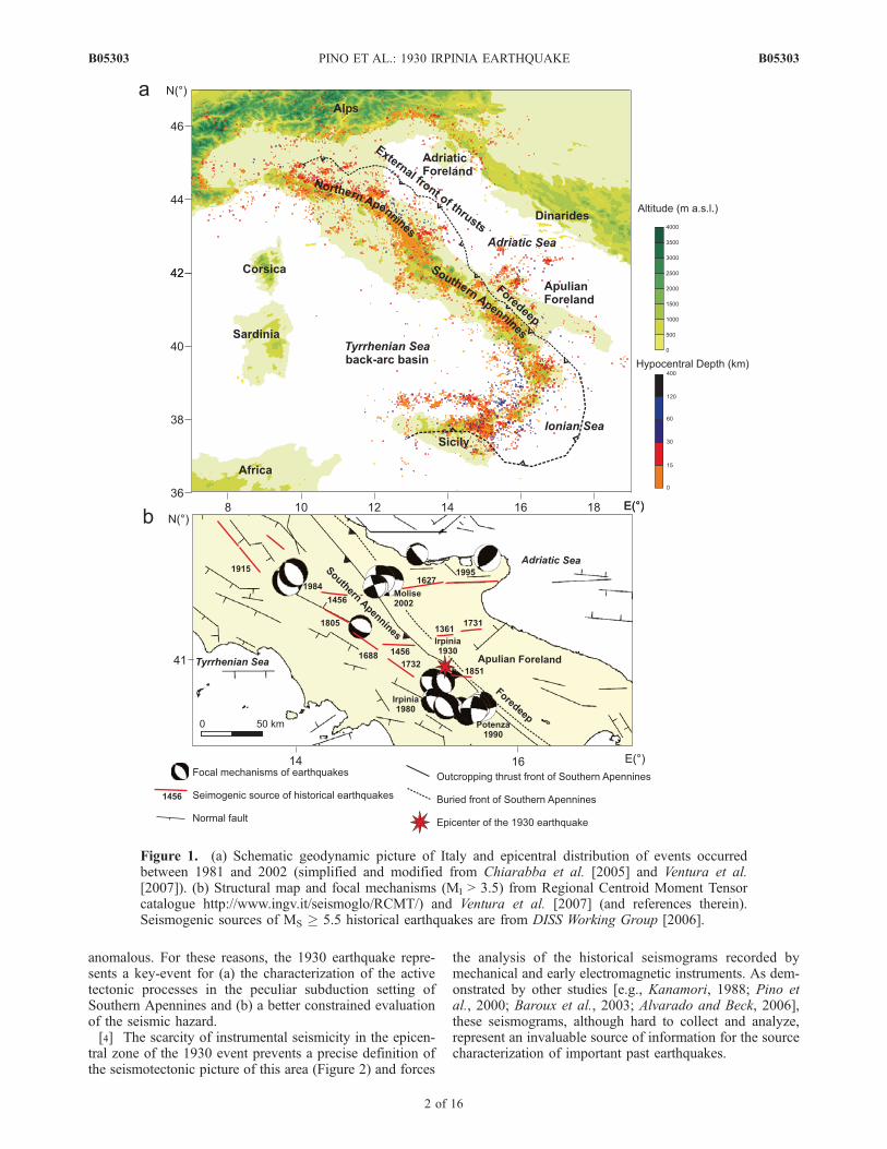
Figure 2. Geological sketch map of the Irpinia region of Southern Apennines. Geology is from Improtaet al. [2003], epicenter and fault of the 1930 earthquake are from this study, faults and directions ofextension are from Hippolyte et al. [1994], epicenters of historical earthquakes are from DISS WorkingGroup [2006], epicenters of 1981–2002 instrumental earthquakes are from Ventura et al. [2007].


3 of 16

B05303

axial zone of Southern Apennines underwent uplift and aNE–SW extensional tectonics, which is responsible forformation of NW–SE striking faults [Cinque et al., 1993;Hippolyte et al., 1994]. This change in the stress regime inPleistocene times is believed to be related to a detachment ofthe slab below the Southern Apennines [Hippolyte et al.,1994; Ventura et al., 2007]. As indicated by boreholebreakouts analysis [Amato and Montone, 1997] and focalmechanism of large earthquakes in Southern Apennines(MW up to 6.9) [Chiarabba et al., 2005], the NE–SWextensional stress regime is still active.[7] The Southern Apennine seismicity concentrates in the

uppermost 15–20 km of the crust along the chain axis(Figure 1a) [Chiarabba et al., 2005; Ventura et al., 2007].Paleoseismological, historical [Valensise and Pantosti,2001b], and slip data on faults affecting Holocene terrains[Hippolyte et al., 1994] confirm the above reported seismo-tectonic picture and reveal that the historical Apennineseismicity also concentrates along the axial zone of the chain(Figure 1b). To east, in the Apulian foreland, the seismicactivity is more widespread, deeper (up to 20–30 km depth),and develops along WNW–ESE to WSW–ENE striking,right-lateral strike-slip faults. These faults are related to thelarger hinge rollback rate of the Adriatic lithosphere to thenorth, with respect to the Apulian lithosphere to the south(Figure 1a) [Di Luccio et al., 2005b; Milano et al., 2005].The seismogenic WNW–ESE striking structures whichaffect the easternmost sectors of the Southern Apennineschain at lat 41�.5, e.g., the fault responsible for the 1456earthquake (Figure 1b) are interpreted as splays of the majorE-W striking faults of the Apulian foreland [Fracassi andValensise, 2007].[8] The 1930 epicentral zone is located in the outer thrust

system of the Southern Apennines, in an area where the

deposits of the thrust sheet–top clastic sequences [Upper-Messinian–Early Pleistocene], the Miocene siliciclasticflysch, the Tertiary sequence of the Lagonegro Basin, andthe vulcanites of the Vulture edifice diffusely outcrop(Figure 2). This area is one of the most active seismiczones of the Southern Apennines and large seismic eventsoccurred in historical and more recent times: earthquakesoccurred in 989, 1466, 1561, 1694, 1702, 1732, 1851, 1857,1930, 1962, and 1980 [Galli et al., 2006]. The 1466, 1694[I0 = X MCS], 1930 [Mw = 6.6] and 1980 [Mw = 6.9]events are the largest ones. In this area, the now inactiveApennine thrusts strike between WNW-ESE and NW-SE.The outcropping normal faults, including that responsiblefor the 1980 earthquake, strike NW-SE and affect the LatePleistocene to Holocene deposits. The available gravitymodeling [Improta et al., 2003] of this area of SouthernApennines shows that the 1930 event epicentral zone over-lies a synform-like structure characterized by an eastwardthickening of the Miocene flysch deposits.

3. Waveform Data and Instrument Responses

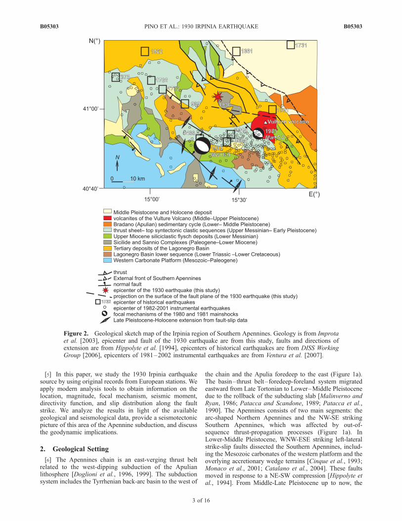
[9] We collected seismograms from the 1930 Irpiniaevent in the frame of the EuroSeismos project [Ferrariand Pino, 2003]. The project itself is aimed at the digitalpreservation of recordings from earthquakes in the Euro-Mediterranean area and relevant station bulletins. It sawinitially the participation of researchers from 15 countries,soon extended to 29 and, by the end of 2005, has beencapable to put together about 25,000 historical seismogramsfrom a list of 611 earthquakes chosen by the participants.More information can be found at http://storing.ingv.it/es_web/index.htm.[10] For the present study we gathered 96 seismograms

from 29 stations (Figure 3). Not all of the recordings aresuitable for waveform digitization and analysis because ofpoor image quality, scarce information on the instrumentresponse, or too slow paper speed to distinguish distinctoscillations. Sometimes the amplitude of first P wavearrivals is too low to be useful. Also, due to amplitudeclipping, some waveforms are usable for source study fromanalysis of first arrivals but not for magnitude estimate.Overall, we digitized 28 seismograms from 15 stations. Theepicentral distances are comprised between 4.7� and 20�,with a single station at 35�, while the azimuthal coverage isabout 190�, with most stations being in 40�, between N325�and N5� (Table 1). The relative high density of stations incentral/northern Europe provides redundant coverage whichis particularly desirable to cross check possible errors in thedata, such as wrong component polarity and instrumentalconstants.[11] When possible, we recovered instrument response

parameters from the original station bulletins relative to thetime of the studied event, otherwise we used the instrumentconstants reported for closest available time period. Theinstrument characteristics of the stations used in the presentanalysis are summarized in Table 2. The set of seismometersconsists of a few electromagnetic Galitzin and mostly ofdifferent types of Wiechert, very common in Europe andproviding good quality recordings. In some cases, theseinstruments have been operating for about a century, until a

Figure 3. The great circle path to the stations where atleast one seismogram was digitized and analyzed.


4 of 16

B05303

few years ago (e.g., Uppsala, up to 1998 [Bodvarsson,1999]) or are still in use (e.g., Gottingen [Ritter, 2002]).

4. Source Analysis

4.1. Location

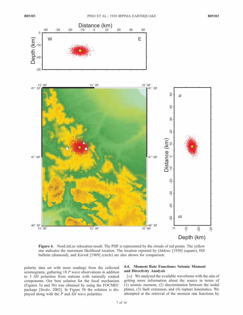
[12] The ISS (International Seismological Summary) bul-letin reports 112 station arrival time observations (109 Pphase and 95 S phase) for the 23 July 1930 Irpiniaearthquake. We used these readings and located the hypo-center of the 23 July 1930 Irpinia earthquake by means ofthe computer program NonLinLoc (NLL) [Lomax, 2005].The code performs a probabilistic location by using animportance-sampling method based on an efficient globalcascading grid-search, to obtain an estimate of the posteriorprobability density function (PDF) in 3D space. The cellwith highest probability is divided in eight cells and thisspace is resampled. This procedure is repeated until atermination criterion is reached. As a result, where theprobability is higher the sampling is denser. The PDF isobtained by means of an equal differential-time formulationof the likelihood function, containing the calculated andobserved differences between two stations, summed overall the pairs of observations. This likelihood definitionmakes the algorithm independent on any origin time esti-mate, then the hypocenter location is reduced to a 3Dproblem, increasing the robustness of the method. Themaximum likelihood point may be assumed as the ‘‘optimal’’location. In case of a single, well defined, maximum, thisrepresents a reliable estimate of the hypocenter. The proce-dure is applied iteratively, with automated and manualreassociation of the arrival phases and elimination of theoutliers. However, due to the definition of the PDF [Lomax,2005], the method is not sensitive to the presence ofoutliers. This feature makes NLL particularly suitable forthe location of historical earthquakes, usually displaying arelatively large number of outliers, which in turn couldresult from phase mis-identification and difficulties inreading arrival times on analog, possibly smoked, paperrecordings, and from poor clock synchronization.[13] We used P and S waves adopting the 1D ak135

model [Kennett et al., 1995] and a specific crustal model

[Basili et al., 1984] for traveltime computations of tele-seismic and local observations, respectively. The predictedtimes were assigned 1 s error in order to account for 3Dstructural complexities. The search for the hypocentralsolution was performed over the region 30�N to 50�N inlatitude, 5�E to 25�E in longitude, down a depth of 700 km.We used arrival time data from the ISS bulletin and appliedthe procedure starting with 100 phases from 57 stations. Byiteratively reassociating the phases and removing all obser-vations with residuals greater than 3 s, the final solution(Figure 4 and Table 3) was obtained after 5 iterations, with63 phases (38 P and 25 S) from 42 stations, with anazimuthal gap of 66�. The zone of highest PDF is wellconstrained in space, with a single maximum locatedapproximately in the center. The RMS associate to thislocation along with the expectation hypocenter and the68% confidence ellipsoid approximation to the PDF arealso reported in Table 3. The ellipsoid represents theformal error of our hypocentral location, which gives anuncertainty of ±3.06 km in depth, ±4.9 km in the NNEdirection and about ±7.7 km in the ESE direction, at anangle of 101�.

4.2. Magnitude

[14] For this earthquake, Karnik [1969] obtained a mag-nitude MS = 6.5, in accordance with the value MS = 61=2reported by Gutenberg and Richter [1954]. More recently, afurther instrumental estimate of MS = 6.6 [Margottini et al.,1993] and an equivalent moment magnitude Me = 6.7[Gasperini et al., 1999] have been also published. By takingadvantage of the relatively high number of seismogramscollected for this study, not available before, we computedthe event magnitude on each suitable waveform. Theinstrument parameters of Table 2 have been used to obtainthe ground displacement from the original seismograms. Aspreviously mentioned, not all the available waveforms couldbe used for evaluating the magnitude. On the contrary, somefor which the magnitude was computed could not be usedfor moment rate retrieval from first P wave arrivals.Because of the multiple sources of error, mainly associatedwith uncertainties in the instrumental parameters, we pre-ferred to compute the magnitude on each waveform, sepa-

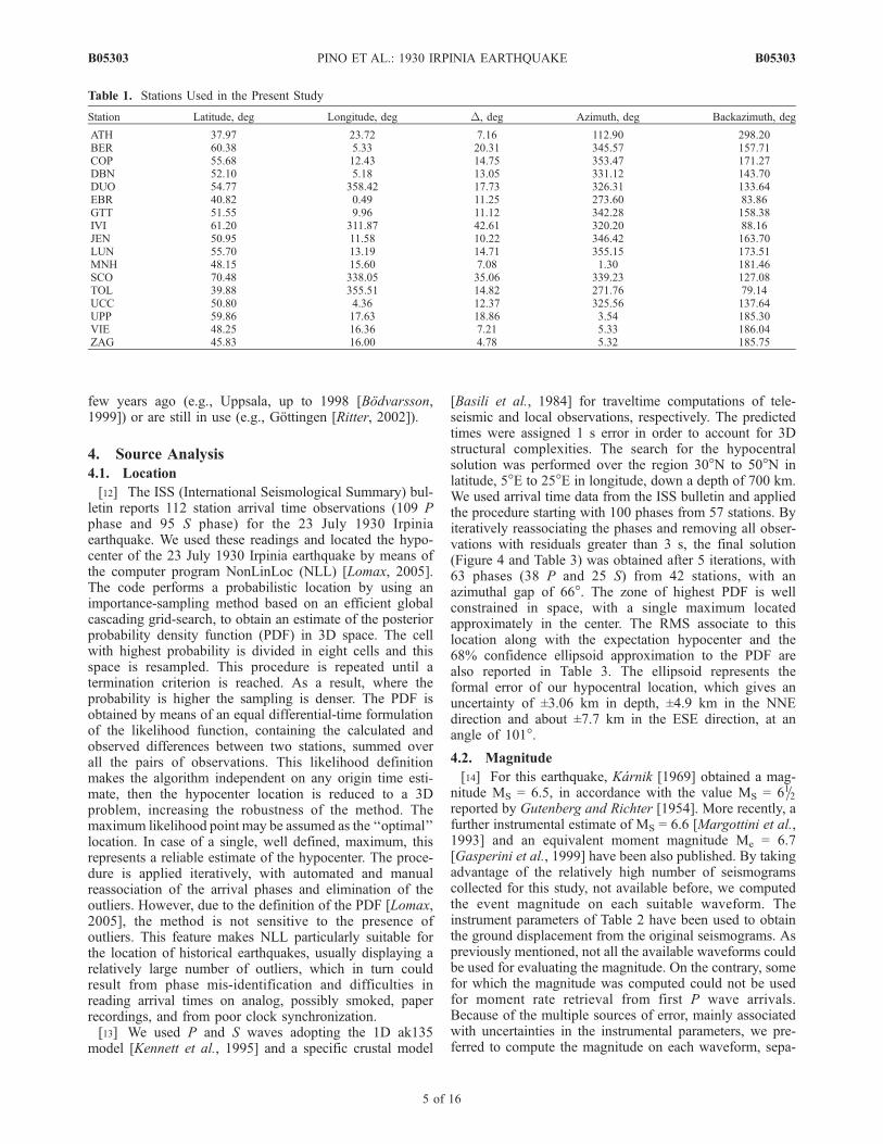
Table 1. Stations Used in the Present Study

Station Latitude, deg Longitude, deg D, deg Azimuth, deg Backazimuth, deg

ATH 37.97 23.72 7.16 112.90 298.20BER 60.38 5.33 20.31 345.57 157.71COP 55.68 12.43 14.75 353.47 171.27DBN 52.10 5.18 13.05 331.12 143.70DUO 54.77 358.42 17.73 326.31 133.64EBR 40.82 0.49 11.25 273.60 83.86GTT 51.55 9.96 11.12 342.28 158.38IVI 61.20 311.87 42.61 320.20 88.16JEN 50.95 11.58 10.22 346.42 163.70LUN 55.70 13.19 14.71 355.15 173.51MNH 48.15 15.60 7.08 1.30 181.46SCO 70.48 338.05 35.06 339.23 127.08TOL 39.88 355.51 14.82 271.76 79.14UCC 50.80 4.36 12.37 325.56 137.64UPP 59.86 17.63 18.86 3.54 185.30VIE 48.25 16.36 7.21 5.33 186.04ZAG 45.83 16.00 4.78 5.32 185.75


5 of 16

B05303

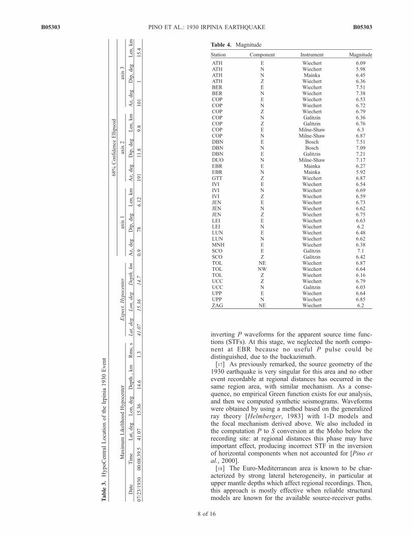
rately. We estimated MS on 41 seismograms obtaining theresults displayed in Table 4. Assuming the mean value asthe magnitude of the 1930 event, we obtained MS = 6.6.

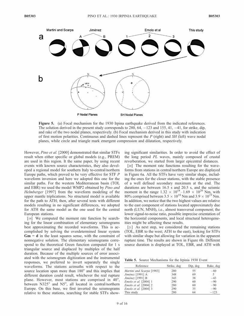
4.3. Focal Mechanism

[15] Several authors have computed a focal mechanismfor the 1930 Irpinia event (Figure 5a and Table 5). Inparticular, the first analysis was made by Martini andScarpa [1983] who inverted 11 first motion polarities fromEuropean stations, obtaining a normal fault mechanism withabout NS tensional axis. Their solution displays a consid-erable amount of strike slip component and nodal planesstriking at N54� and N280�. Successively, Jimenez [1991]inverted horizontal waveforms of single station data from

JEN (Germany). She tested two different crustal models inthe source region, deriving different solutions: one almostpure strike slip and the other, more stable, displaying anormal fault with important strike slip component. Morerecently, Emolo et al. [2004] used 8 polarities from Martiniand Scarpa [1983] data set and applied a couple of differentmethods, obtaining two solutions only differing by 10� instrike with roughly ESE–WNW striking planes. Based onforward modeling of the intensity field, they elaborate athird solution displaying same planes strike but substantiallydifferent dip, proposing the south dipping surface as the oneassociate to the rupture. It should be noted that the latterfocal mechanism visibly does not satisfy the polarities ofMartini and Scarpa [1983]. We integrated the first motion

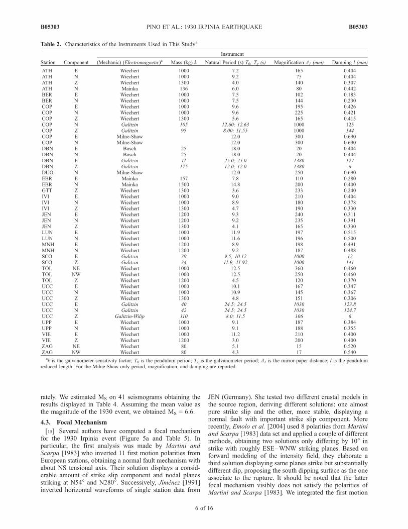
Table 2. Characteristics of the Instruments Used in This Studya

Station Component

Instrument

(Mechanic) (Electromagnetic)a Mass (kg) k Natural Period (s) T0; Tg (s) Magnification A1 (mm) Damping l (mm)

ATH E Wiechert 1000 7.2 165 0.404ATH N Wiechert 1000 9.2 75 0.404ATH Z Wiechert 1300 4.0 140 0.307ATH N Mainka 136 6.0 80 0.442BER E Wiechert 1000 7.5 102 0.183BER N Wiechert 1000 7.5 144 0.230COP E Wiechert 1000 9.6 195 0.426COP N Wiechert 1000 9.6 225 0.421COP Z Wiechert 1300 5.6 165 0.415COP N Galitzin 105 12.60; 12.63 1000 125COP Z Galitzin 95 8.00; 11.55 1000 144COP E Milne-Shaw 12.0 300 0.690COP N Milne-Shaw 12.0 300 0.690DBN E Bosch 25 18.0 20 0.404DBN N Bosch 25 18.0 20 0.404DBN E Galitzin 11 25.0; 25.0 1380 127DBN Z Galitzin 175 12.0; 12.0 1380 6DUO N Milne-Shaw 12.0 250 0.690EBR E Mainka 157 7.8 110 0.280EBR N Mainka 1500 14.8 200 0.400GTT Z Wiechert 1300 3.6 233 0.240IVI E Wiechert 1000 9.0 210 0.404IVI N Wiechert 1000 8.9 180 0.378IVI Z Wiechert 1300 4.7 190 0.330JEN E Wiechert 1200 9.3 240 0.311JEN N Wiechert 1200 9.2 235 0.391JEN Z Wiechert 1300 4.1 165 0.330LUN E Wiechert 1000 11.9 197 0.515LUN N Wiechert 1000 11.6 196 0.500MNH E Wiechert 1200 8.9 198 0.491MNH N Wiechert 1200 9.2 187 0.488SCO E Galitzin 39 9.5; 10.12 1000 12SCO Z Galitzin 34 11.9; 11.92 1000 141TOL NE Wiechert 1000 12.5 360 0.460TOL NW Wiechert 1000 12.5 250 0.460TOL Z Wiechert 1200 4.5 120 0.370UCC E Wiechert 1000 10.1 167 0.347UCC N Wiechert 1000 10.9 145 0.367UCC Z Wiechert 1300 4.8 151 0.306UCC E Galitzin 40 24.5; 24.5 1030 123.8UCC N Galitzin 42 24.5; 24.5 1030 124.7UCC Z Galitzin-Wilip 110 8.0; 11.5 106 6UPP E Wiechert 1000 9.1 187 0.384UPP N Wiechert 1000 9.1 188 0.355VIE E Wiechert 1000 11.2 210 0.400VIE Z Wiechert 1200 3.0 200 0.400ZAG NE Wiechert 80 5.1 15 0.520ZAG NW Wiechert 80 4.3 17 0.540

ak is the galvanometer sensitivity factor; T0 is the pendulum period; Tg is the galvanometer period; A1 is the mirror-paper distance; l is the pendulumreduced length. For the Milne-Shaw only period, magnification, and damping are reported.


6 of 16

B05303

polarity data set with more readings from the collectedseismograms, gathering 18 P wave observations in additionto 3 SH polarities from stations with naturally rotatedcomponents. Our best solution for the focal mechanism(Figures 5a and 5b) was obtained by using the FOCMECpackage [Snoke, 2002]. In Figure 5b the solution is dis-played along with the P and SH wave polarities.

4.4. Moment Rate Functions: Seismic Momentand Directivity Analysis

[16] We analyzed the available waveforms with the aim ofgetting more information about the source in terms of(1) seismic moment, (2) discrimination between the nodalplanes, (3) fault extension, and (4) rupture kinematics. Weattempted at the retrieval of the moment rate functions by

Figure 4. NonLinLoc relocation result. The PDF is represented by the clouds of red points. The yellowstar indicates the maximum likelihood location. The location reported by Oddone [1930] (square), ISSbulletin (diamond), and Karnik [1969] (circle) are also shown for comparison.


7 of 16

B05303

inverting P waveforms for the apparent source time func-tions (STFs). At this stage, we neglected the north compo-nent at EBR because no useful P pulse could bedistinguished, due to the backazimuth.[17] As previously remarked, the source geometry of the

1930 earthquake is very singular for this area and no otherevent recordable at regional distances has occurred in thesame region area, with similar mechanism. As a conse-quence, no empirical Green function exists for our analysis,and then we computed synthetic seismograms. Waveformswere obtained by using a method based on the generalizedray theory [Helmberger, 1983] with 1-D models andthe focal mechanism derived above. We also included inthe computation P to S conversion at the Moho below therecording site: at regional distances this phase may haveimportant effect, producing incorrect STF in the inversionof horizontal components when not accounted for [Pino etal., 2000].[18] The Euro-Mediterranean area is known to be char-

acterized by strong lateral heterogeneity, in particular atupper mantle depths which affect regional recordings. Then,this approach is mostly effective when reliable structuralmodels are known for the available source-receiver paths.T

able

3.HypoCentral

LocationoftheIrpinia

1930Event

Maxim

um

LikelihoodHypocenter

Expect.Hypocenter

68%

Confidence

Ellipsoid

axis1

axis2

axis3

Date

Tim

eLat,deg

Lon,deg

Depth

,km

Rms,s

Lat,deg

Lon,deg

Depth,km

Az,

deg

Dip,deg

Len,km

Az,

deg

Dip,deg

Len,km

Az,

deg

Dip,deg

Len,km

07/23/1930

00:08:39.5

41.07

15.36

14.6

1.3

41.07

15.36

14.7

0.9

78

6.12

191

11.8

9.8

101

115.4

Table 4. Magnitude

Station Component Instrument Magnitude

ATH E Wiechert 6.09ATH N Wiechert 5.98ATH N Mainka 6.45ATH Z Wiechert 6.36BER E Wiechert 7.51BER N Wiechert 7.38COP E Wiechert 6.53COP N Wiechert 6.72COP Z Wiechert 6.79COP N Galitzin 6.36COP Z Galitzin 6.76COP E Milne-Shaw 6.3COP N Milne-Shaw 6.87DBN E Bosch 7.51DBN N Bosch 7.09DBN E Galitzin 7.21DUO N Milne-Shaw 7.17EBR E Mainka 6.27EBR N Mainka 5.92GTT Z Wiechert 6.87IVI E Wiechert 6.54IVI N Wiechert 6.69IVI Z Wiechert 6.59JEN E Wiechert 6.73JEN N Wiechert 6.62JEN Z Wiechert 6.75LEI E Wiechert 6.63LEI N Wiechert 6.2LUN E Wiechert 6.48LUN N Wiechert 6.62MNH E Wiechert 6.38SCO E Galitzin 7.1SCO Z Galitzin 6.42TOL NE Wiechert 6.87TOL NW Wiechert 6.64TOL Z Wiechert 6.16UCC Z Wiechert 6.79UCC N Galitzin 6.03UPP E Wiechert 6.64UPP N Wiechert 6.85ZAG NE Wiechert 6.2


8 of 16

B05303

However, Pino et al. [2000] demonstrated that similar STFsresult when either specific or global models (e.g., PREM)are used in this region. It the same paper, by using recentevents with known source characteristics, they also devel-oped a regional model for southern Italy to-central/northernEurope paths, which proved to be very effective for STF Pwaveform inversion and here we adopted this one for thesimilar paths. For the western Mediterranean basin (TOLand EBR) we used the model WMP2 obtained by Pino andHelmberger [1997] from the waveform modeling of theupper mantle triplications. No structural model is availablefor the path to ATH; then, after several tests with differentmodels resulting in no significant differences, we adoptedfor ATH the same model as the one used for the centralEuropean stations.[19] We computed the moment rate function by search-

ing for the linear combination of elementary seismogramsbest approximating the recorded waveforms. This is ac-complished by solving the overdetermined linear systemGm = d in the least squares sense, with the constraint ofnonnegative solution. The elementary seismograms corre-spond to the theoretical Green function computed for 1 striangular source and displaced by multiples of the halfduration. Because of the multiple sources of error associ-ated with the seismogram digitization and the instrumentalresponses, we preferred to invert separately the singlewaveforms. The stations azimuths with respect to thesource location span more than 180� and this implies thatdifferent duration could result, whichever the real ruptureplane. However, most stations are comprised in 40�,between N325� and N5�, all located in central/northernEurope. On this base, we first inverted the seismogramsrelative to these stations, searching for stable STFs show-

ing significant similarities. In order to avoid the effect ofthe long period PL waves, mainly composed of crustalreverberation, we started from larger epicentral distances.[20] The moment rate functions resulting for the wave-

forms from stations in central/northern Europe are displayedin Figure 6a. All the STFs have very similar shape, includ-ing the ones for the closer stations, with the stable presenceof a well defined secondary maximum at the end. Thedurations are between 16.5 s and 20.5 s, and the seismicmoment in the range 1.32 � 1018–1.69 � 1020 Nm, with80% comprised between 3.5� 1018 Nm and 3.9� 1019 Nm.In addition, we notice that the two highest values are relativeto the east component of stations located approximately duenorth (LUN, MNH), i.e., almost transversal component; thelower signal-to-noise ratio, possible imprecise orientation ofthe horizontal components, and local structural heterogene-ities might be affecting these results.[21] As next step, we considered the remaining stations

(TOL, EBR to the west; ATH to the east), looking for STFswith similar shape but allowing for variation in the apparentrupture time. The results are shown in Figure 6b. Differentsource duration is displayed at TOL, EBR, and ATH with

Figure 5. (a) Focal mechanism for the 1930 Irpina earthquake derived from the indicated references.The solution derived in the present study corresponds to 280, 64, �123 and 155, 41, �41, for strike, dip,and rake of the two nodal planes, respectively. (b) Focal mechanism derived in this study with indicationof first motion polarities. Continuous and dashed lines represent the P (right) and SH (left) wave nodalplanes, while circle and triangle mark emergent compression and dilatation, respectively.

Table 5. Source Mechanisms for the Irpinia 1930 Event

Reference Strike, deg Dip, deg Rake, deg

Martini and Scarpa [1983] 280 55 �60Jimenez [1991] A 348 69 5Jimenez [1991] B 343 38 �43Emolo et al. [2004] 1 290 60 �90Emolo et al. [2004] 2 280 60 �90Emolo et al. [2004] 3 290 35 �90This study 280 64 �123


9 of 16

B05303

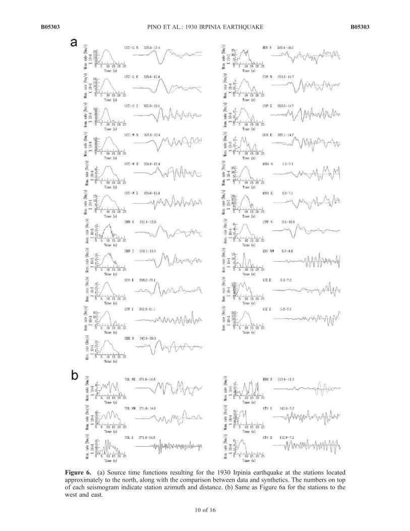
Figure 6. (a) Source time functions resulting for the 1930 Irpinia earthquake at the stations locatedapproximately to the north, along with the comparison between data and synthetics. The numbers on topof each seismogram indicate station azimuth and distance. (b) Same as Figure 6a for the stations to thewest and east.


10 of 16

B05303

respect to station to the north, with about 22 s to the westand 11 s to the east, with M0 in a comparable range. Theoverall variability of the seismic moment for the closerstations is probably due to the structural model approxima-tion and the effect of PL waves. As a matter of fact, thelargest scatter results at shorter distances. In particular, M0

relative to stations located at less than 12� are distributed inan approximately double range than the ones beyond 12�.[22] By dropping the results for the east component of the

stations located almost due north (LUN, MNH, VIE), weassumed the average value as a good estimate of the seismicmoment getting 1.16 (±0.43) � 1019 Nm, corresponding toMW = 6.64. This results is in very good agreement with thecomputed MS (Table 4), but also very similar to whatobtained by Gasperini et al. [1999] from the analysis ofthe felt reports.[23] As for the apparent durations of the resulting STFs, a

clear decrease from west to east is displayed. This patterncould derive from a rupture along an approximately E-Wstriking plane, with mostly unilateral rupture propagationtoward east. If true, this would candidate the north dippingplane (strike N280�) of the focal mechanism as the oneassociated to the fault. We tested this hypothesis by invert-ing the deduced durations for fault parameters. We adopteda simple Haskell [1964] unilateral rupture of length L, withconstant velocity vr. Then, the apparent duration is given by:

t ¼ Lð1=vr � cosqr=cÞ ð1Þ

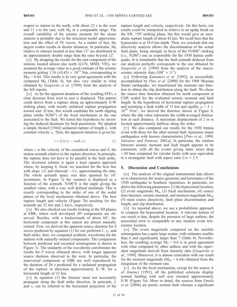
where c is the velocity of the considered waves and qr thestation azimuth relative to the rupture direction. In principle,the rupture does not have to be parallel to the fault strike.The inversion scheme is again a least squares approachwhere, by keeping qr fixed, we searched for the best linewith slope 1/L and intercept �1/vr approximating the data.The whole azimuth space was then spanned by 10�increments. In Figure 7a the variance is displayed as afunction of the azimuth. N100�E is the angle giving thesmallest value, with a very well defined minimum. This isexactly corresponding to the strike of one of the nodalplanes of the focal mechanism obtained above. The bestrupture length and velocity (Figure 7b) resulting for thisazimuth are 32 km and 2 km/s, respectively.[24] We also checked our results looking at the SH phases

at EBR, where well developed SH components are ob-served. Besides, with a backazimuth of about 84�, thehorizontal component at this station are almost naturallyrotated. First, we derived the apparent source duration for Swaves predicted by equation (1) for our preferred L, vr, andfault strike; then, we computed synthetic waveforms for thestations with naturally rotated components. The comparisonbetween predicted and recorded seismograms is shown inFigure 7c. The similarity of the waveforms corroborates theresults for P waves obtained above, with longer apparentsource duration observed to the west. In particular, thetransversal component at EBR are well reproduced bythe duration of 26 s predicted for a unilateral propagationof the rupture in direction approximately E–W, for ahorizontal length of 32 km.[25] In equation (1) the fracture must not necessarily

propagate along the fault strike direction. In principle, Land vr can be referred to the horizontal projection of the

rupture length and velocity, respectively. On this basis, ourresults could be interpreted as relative to an updip break onthe SW, 158�-striking plane, but this would give an unre-alistic rupture length of about 42 km. We recall here that thehypocenter is at 14.6 km depth. Then, we conclude that ourdirectivity analysis allows the discrimination of the actualfault plane, being strongly in favor of the N100E�-striking(i.e., N280�) one as responsible for the 1930 Irpinia earth-quake. It is remarkable that the fault azimuth deduced fromour analysis perfectly corresponds to the one obtained byGasperini et al. [1999] from the analysis of the macro-seismic intensity data (108� ± 11�).[26] Following Kanamori et al. [1992], as successfully

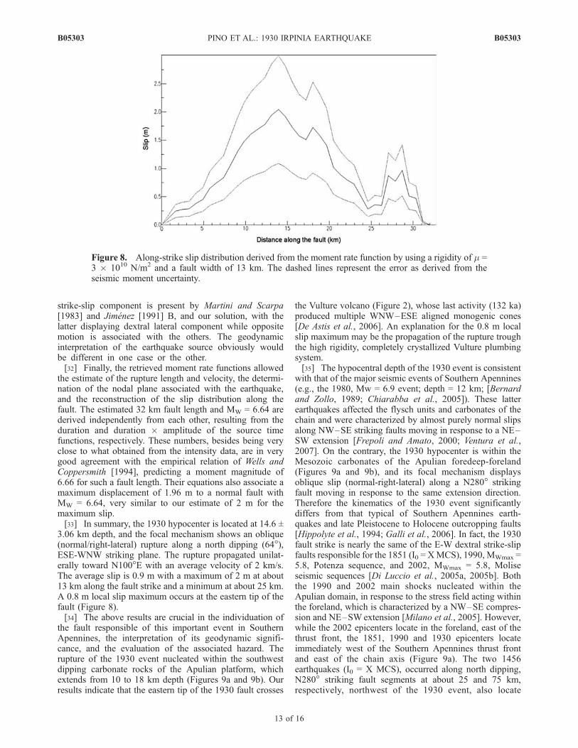
accomplished by Pino et al. [2000] for the 1908 MessinaStraits earthquake, we transformed the moment rate func-tion to obtain the slip distribution along the fault. We chosethe source time function obtained for north component atCOP, scaled for the evaluated seismic moment and faultlength. In the hypothesis of horizontal rupture propagationand assuming a fault width of 13 km and rigidity m = 3 �1010 N/m2, we derived the function shown in Figure 8,where the slip value represents the width-averaged disloca-tion at each distance. A maximum displacement of 2 m islocated approximately halfway along the strike.[27] We also compared our results for the 1930 Irpinia

event with those for the other normal fault Apenninic majorearthquakes with known characteristics [Pino et al., 1999;Valensise and Pantosti, 2001a]. In particular, the relationbetween seismic moment and fault length appears to beconsistent, with all the events giving static stress drop�30 bars computed for circular faults with area equivalentto a rectangular fault with aspect ratio L/w = 2.5.

5. Discussion and Conclusions

[28] The analysis of the original instrumental data allowsus to characterize the source geometry and kinematics of the1930 earthquake in Southern Apennines. In particular, wederive the following parameters: (1) the hypocentral location,(2) event magnitude MS, (3) focal mechanism, (4) sourcetime function, seismic moment, and moment magnitude MW,(5) main source directivity, fault plane discrimination andlength, and slip distribution.[29] As reported above, we use a probabilistic approach

to compute the hypocentral location. A relevant feature ofour result is that, despite the presence of large outliers, theassociated error is comparable to any modern event tele-seismic location.[30] The event magnitude computed on the suitable

seismograms has a quite large scatter, with estimates smallerthan 6 and significantly larger than 7 (Table 4). Neverthe-less, the resulting average MS = 6.6 is in good agreementwith what computed by other authors and with the equiv-alent magnitude derived from intensity data [Gasperini etal., 1999]. Moreover, it is almost coincident with our resultfor the moment magnitude (MW = 6.64) obtained from theintegration of the moment rate.[31] As for the focal mechanism, except for the source A

of Jimenez [1991], all the published solutions displaynormal faulting with null axis oriented approximatelyE-W (Figure 5a). More in detail, the sources from Emoloet al. [2004] are purely normal fault whereas a significant


11 of 16

B05303

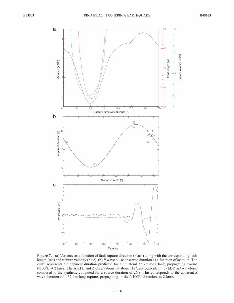
Figure 7. (a) Variance as a function of fault rupture direction (black) along with the corresponding faultlength (red) and rupture velocity (blue). (b) P wave pulse observed duration as a function of azimuth. Thecurve represents the apparent duration predicted for a unilateral 32 km-long fault, propagating towardN100�E at 2 km/s. The ATH E and Z observations, at about 112�, are coincident. (c) EBR SH waveformcompared to the synthetic computed for a source duration of 26 s. This corresponds to the apparent Swave duration of a 32 km-long rupture, propagating in the N100E� direction, at 2 km/s.


12 of 16

B05303

strike-slip component is present by Martini and Scarpa[1983] and Jimenez [1991] B, and our solution, with thelatter displaying dextral lateral component while oppositemotion is associated with the others. The geodynamicinterpretation of the earthquake source obviously wouldbe different in one case or the other.[32] Finally, the retrieved moment rate functions allowed

the estimate of the rupture length and velocity, the determi-nation of the nodal plane associated with the earthquake,and the reconstruction of the slip distribution along thefault. The estimated 32 km fault length and MW = 6.64 arederived independently from each other, resulting from theduration and duration � amplitude of the source timefunctions, respectively. These numbers, besides being veryclose to what obtained from the intensity data, are in verygood agreement with the empirical relation of Wells andCoppersmith [1994], predicting a moment magnitude of6.66 for such a fault length. Their equations also associate amaximum displacement of 1.96 m to a normal fault withMW = 6.64, very similar to our estimate of 2 m for themaximum slip.[33] In summary, the 1930 hypocenter is located at 14.6 ±

3.06 km depth, and the focal mechanism shows an oblique(normal/right-lateral) rupture along a north dipping (64�),ESE-WNW striking plane. The rupture propagated unilat-erally toward N100�E with an average velocity of 2 km/s.The average slip is 0.9 m with a maximum of 2 m at about13 km along the fault strike and a minimum at about 25 km.A 0.8 m local slip maximum occurs at the eastern tip of thefault (Figure 8).[34] The above results are crucial in the individuation of

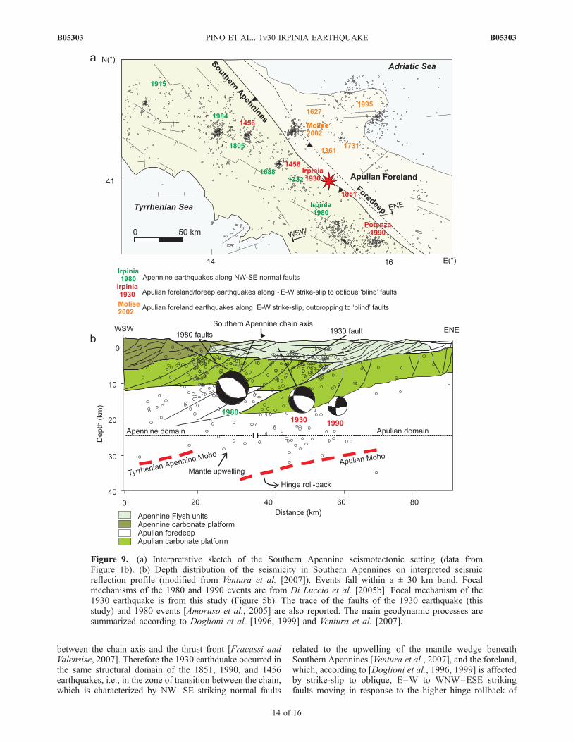
the fault responsible of this important event in SouthernApennines, the interpretation of its geodynamic signifi-cance, and the evaluation of the associated hazard. Therupture of the 1930 event nucleated within the southwestdipping carbonate rocks of the Apulian platform, whichextends from 10 to 18 km depth (Figures 9a and 9b). Ourresults indicate that the eastern tip of the 1930 fault crosses

the Vulture volcano (Figure 2), whose last activity (132 ka)produced multiple WNW–ESE aligned monogenic cones[De Astis et al., 2006]. An explanation for the 0.8 m localslip maximum may be the propagation of the rupture troughthe high rigidity, completely crystallized Vulture plumbingsystem.[35] The hypocentral depth of the 1930 event is consistent

with that of the major seismic events of Southern Apennines(e.g., the 1980, Mw = 6.9 event; depth = 12 km; [Bernardand Zollo, 1989; Chiarabba et al., 2005]). These latterearthquakes affected the flysch units and carbonates of thechain and were characterized by almost purely normal slipsalong NW–SE striking faults moving in response to a NE–SW extension [Frepoli and Amato, 2000; Ventura et al.,2007]. On the contrary, the 1930 hypocenter is within theMesozoic carbonates of the Apulian foredeep-foreland(Figures 9a and 9b), and its focal mechanism displaysoblique slip (normal-right-lateral) along a N280� strikingfault moving in response to the same extension direction.Therefore the kinematics of the 1930 event significantlydiffers from that typical of Southern Apennines earth-quakes and late Pleistocene to Holocene outcropping faults[Hippolyte et al., 1994; Galli et al., 2006]. In fact, the 1930fault strike is nearly the same of the E-W dextral strike-slipfaults responsible for the 1851 (I0 = XMCS), 1990, MWmax =5.8, Potenza sequence, and 2002, MWmax = 5.8, Moliseseismic sequences [Di Luccio et al., 2005a, 2005b]. Boththe 1990 and 2002 main shocks nucleated within theApulian domain, in response to the stress field acting withinthe foreland, which is characterized by a NW–SE compres-sion and NE–SW extension [Milano et al., 2005]. However,while the 2002 epicenters locate in the foreland, east of thethrust front, the 1851, 1990 and 1930 epicenters locateimmediately west of the Southern Apennines thrust frontand east of the chain axis (Figure 9a). The two 1456earthquakes (I0 = X MCS), occurred along north dipping,N280� striking fault segments at about 25 and 75 km,respectively, northwest of the 1930 event, also locate

Figure 8. Along-strike slip distribution derived from the moment rate function by using a rigidity of m =3 � 1010 N/m2 and a fault width of 13 km. The dashed lines represent the error as derived from theseismic moment uncertainty.


13 of 16

B05303

between the chain axis and the thrust front [Fracassi andValensise, 2007]. Therefore the 1930 earthquake occurred inthe same structural domain of the 1851, 1990, and 1456earthquakes, i.e., in the zone of transition between the chain,which is characterized by NW–SE striking normal faults

related to the upwelling of the mantle wedge beneathSouthern Apennines [Ventura et al., 2007], and the foreland,which, according to [Doglioni et al., 1996, 1999] is affectedby strike-slip to oblique, E–W to WNW–ESE strikingfaults moving in response to the higher hinge rollback of

Figure 9. (a) Interpretative sketch of the Southern Apennine seismotectonic setting (data fromFigure 1b). (b) Depth distribution of the seismicity in Southern Apennines on interpreted seismicreflection profile (modified from Ventura et al. [2007]). Events fall within a ± 30 km band. Focalmechanisms of the 1980 and 1990 events are from Di Luccio et al. [2005b]. Focal mechanism of the1930 earthquake is from this study (Figure 5b). The trace of the faults of the 1930 earthquake (thisstudy) and 1980 events [Amoruso et al., 2005] are also reported. The main geodynamic processes aresummarized according to Doglioni et al. [1996, 1999] and Ventura et al. [2007].


14 of 16

B05303

the Adriatic lithosphere with respect to the Apulian litho-sphere (Figure 9b). The seismic belt depicted by the 1456,1851, 1930, and 1990 earthquakes is within this back-rolling, hinge zone of the Apulian lithosphere, which ischaracterized by WNW–ESE to E–W striking faults thatdate back to the Mesozoic age [Chilovi et al., 2000]. Wepropose that the above reported events developed alongthese faults, which, on the basis of the 1930 and 1990 focalmechanisms, move with oblique or strike-slip kinematicsdepending on depth and locally prevailing Apennines orforeland stress fields. Finally, it is worth nothing that surfacefailure is not reported for any of these earthquakes, suggest-ing that the seismogenic faults underlying the externalsector of Southern Apennines mainly affect the Apuliancarbonates. This observation rules out the possibility thatthe 1456, 1930, and 1990 events represent the re-activationof the outcropping WNW–ESE striking strike-slip faultsthat dissected the flysch and underlying carbonates of theSouthern Apennines chain in Lower-Middle Pleistocene[Catalano et al., 2004] (see also section 2). We concludethat the sector of the Apulian foreland-foredeep underlyingthe Southern Apennines chain is affected by WNW–ESE‘‘blind’’ faults capable of highly destructive events like the1930 earthquake. Geophysical and geochemical investiga-tions are needed to detect the possible occurrence of otherseismogenic ‘‘blind’’ structures.

[36] Acknowledgments. We thank R. Console, R. Scarpa, andJ. Batllo for comments and suggestions, L. Arcoraci for help with seismo-grams digitations, and C. Piromallo, L. Improta, F.R. Cinti, U. Fracassi,R. Di Giovambattista, and G. Milano for the numerous discussions on thegeodynamic significance of the Southern Apennine seismicity. This work issupported by INGV funds.

ReferencesAlvarado, P., and S. Beck (2006), Source characterization of the San Juan(Argentina) crustal earthquakes of 15 January 1944 (Mw 7.0) and 11 June1952 (Mw 6.8), Earth Planet. Sci. Lett., doi:10.1016/j.epsl.2006.01.015.

Amato, A., and P. Montone (1997), Present day stress field and activetectonics in southern peninsular Italy, Geophys. J. Int., 130, 519–534.

Amoruso, A., L. Crescentini, and R. Scarpa (2005), Faulting geometry forthe complex 1980 Campania-Lucania earthquake from levelling data,Geoph. J. Int., 162, 156–168, doi:10.1111/j.1365-246X.2005.02652.x.

Baroux, E., N. A. Pino, G. Valensise, O. Scotti, and M. E. Cushing (2003),Source parameters of the 11 June 1909, Lambesc (Provence, southeasternFrance) earthquake: A reappraisal based on macroseismic, seismological,and geodetic observations, J. Geophys. Res., 108(B9), 2454, doi:10.1029/2002JB002348.

Basili, A., G. Smriglio, and G. Valensise (1984), Procedure di determina-zione ipocentrale in uso presso l’Istituto Nazione di Geofisica, Atti IIIConvegno G.N.G.T.S., Roma, 875–884.

Bernard, P., and A. Zollo (1989), The Irpinia (Italy) 1980 earthquake:Detailed analysis of a complex normal faulting, J. Geophys. Res.,94(B2), 1631–1647.

Bodvarsson, R. (1999), The new Swedish seismic network, ORFEUSNewslett., l(3), 22.

Catalano, S., C. Monaco, L. Tortorici, W. Paltrinieri, and N. Steel (2004),Neogene-quaternary tectonic evolution of the southern Apennines, Tec-tonics, 23, TC2003, doi:10.1029/2003TC001512.

Chiarabba, C., L. Jovane, and R. Di Stefano (2005), A new view of Italianseismicity using 20 years of instrumental recordings, Tectonophysics,395, 251–268, doi:1016/j.tecto.2004.09.013.

Chilovi, C., A. J. De Feyter, and A. Pompucci (2000), Wrench zone reacti-vation in the Adriatic Block: The example of the Mattinata fault system(SE Italy), Boll. Soc. Geol. It., 119, 3–8.

Cinque, A., E. Patacca, P. Scandone, and M. Tozzi (1993), Quaternarykinematic evolution of the Southern Apennines. Relationship betweensurface geological features and deep lithospheric structures, Ann. Geo-phys., 36, 249–260.

De Astis, G., P. D. Kempton, A. Peccerillo, and T. W. Wu (2006), Traceelement and isotopic variations from Mt. Vulture to Campanian volca-

noes: Constraints for slab detachment and mantle inflow beneath south-ern Italy, Contrib. Mineral. Petrol., 151, 331–351, doi:10.1007/s00410-006-0062-y.

Di Luccio, F., E. Fukuyama, and N. A. Pino (2005a), The 2002 Moliseearthquake sequence: What can we learn about the tectonics of SouthernItaly?, Tectonophysics, 405, 141–154, doi:10.1016/j.tecto2005.05.024.

Di Luccio, F., A. Piscini, N. A. Pino, and G. Ventura (2005b), Reactivationof deep faults beneath Southern Apennines: Evidence from the 1990–1991 Potenza seismic sequences, Terra Nova, 17, 586–590, doi:10.1111/j.1365-3121.2005.00653.x.

DISS Working Group (2006), Database of Individual Seismogenic Sources(DISS), Version 3.0.2: A compilation of potential sources for earthquakeslarger than M 5.5 in Italy and surrounding areas. http://www.ingv.it/DISS/

Doglioni, C., P. Harabaglia, G. Martinelli, F. Mongelli, and G. Zito (1996),A geodynamic model of the southern Apennines, Terra Nova, 8, 540–547.

Doglioni, C., E. Gueguen, P. Harabaglia, and F. Mongelli (1999), On theorigin of W-directed subduction zones and applications to the westernMediterranean, Geol. Soc. Am. Spec. Pap., 156, 541–561.

Emolo, A., G. Iannaccone, A. Zollo, and A. Gorini (2004), Inferences onthe source mechanisms of the 1930 Irpinia (southern Italy) earthquakefrom simulations of the kinematic rupture process, Ann. Geophys., 47,1743–1754.

Ferrari, G., and N. A. Pino (2003), Euroseismos 2002-2003, a project forsaving and studying historical seismograms in the Euro-Mediterraneanarea, Geophys. Res. Abstr., 5, 05274.

Fracassi, U., and G. Valensise (2007), Unveiling the sources of the cata-strophic 1456 multiple earthquake: Hints to an unexplored tectonic me-chanism in southern Italy, Bull. Seismol. Soc. Am., 97, 725 –748,doi:10.1785/0120050250.

Frepoli, A., and A. Amato (2000), Stress tensor orientation in peninsularItaly from background seismicity, Tectonophysics, 317, 109–124.

Galli, V. Bosi, S. Piscitelli, A. Giocoli, and V. Scionti (2006), Late Holoceneearthquakes in southern Apennine, paleoseismology of the Caggiano fault,Int. J. Earth. Sci., 95, 855–870, doi:10.1007/s00531-005-0066-2.

Gasperini, P., F. Bernardini, G. Valensise, and E. Boschi (1999), Definingseismogenic sources from historical felt reports, Bull. Seismol. Soc. Am.,78, 94–110.

Gutenberg, B., and C. F. Richter (1954), Seismicity of the Earth and Asso-ciated Phenomena, 2nd ed., Princeton University Press, Princeton, NewJersey.

Haskell, N. A. (1964), Total energy and energy spectral density of elasticwave radiation from propagating faults, Bull. Seismol. Soc. Am., 54,1811–1842.

Helmberger, D. V. (1983), Theory and application of synthetics seismo-grams, in Earthquakes: Observation, Theory and Interpretation, Proc.Int. Sch. Phys. Enrico Fermi, Course LXXXV, edited by H. Kanamoriand E. Boschi, pp. 174–222, North-Holland, Amsterdam.

Hippolyte, J. C., J. Angelier, and F. Roure (1994), A major geodynamicchange revealed by Quaternary stress patterns in the Southern Apennines(Italy), Tectonophysics, 230, 199–210.

Improta, L., M. Bonagura, P. Capuano, and G. Iannaccone (2003), Anintegrated geophysical investigation of the upper crust in the epicentralarea of the 1980, Ms = 6.9, Irpinia earthquake (Southern Italy), Tectono-physics, 361, 139–169, doi:10.1016/S0040-1951(02)00588-7.

Jenny, S., S. Goes, D. Giardini, and H. G. Kahle (2006), Seismic potentialof Southern Italy, Tectonophysics, 415, 81–101, doi:10.1016/jtecto.2005.12.003.

Jimenez, E. (1991), Focal mechanism of some European earthquakesfrom the analysis of single station long-periods record, in Seismicity,Seismotectonics and Seismic Risk of the Ibero-Maghrebian Region, editedby J. Mezcua and A. Udias, pp. 87–96, Monografia N� 8, IGN, Madrid.

Kanamori, H. (1988), Importance of historical seismograms for geophysicalresearch, in Historical Seismograms and Earthquakes of the World, editedby W. H. K. Lee et al., pp. 16–33, Academic Press, San Diego.

Kanamori, H., H.-K. Thio, D. Dreger, E. Hauksson, and T. Heaton (1992),Initial inverstigation of the Landers, California earthquake of 28 June1992 using TERRAscope, Geophys. Res. Lett., 19(22), 2267–2270.

Karnik, V. (1969), Seismicity of the European Area, Part 1, D, ReidelPublishing Company, Doordrecht, Holland.

Kennett, B. L. N, E. R. Engdahl, and R. Buland (1995), Constraints onseismic velocities in the Earth from travel times, Geophys. J. Int., 122,108–124.

Lomax, A. (2005), A reanalysis of the hypocentral location and relatedobservations for the great 1906 California earthquake, Bull. Seismol.Soc. Am., 95, 861–877, doi:10.1785/0120040141.

Malinverno, A., and B. F. Ryan (1986), Extension in the Tyrrhenian Seaand shortening in the Apennines as result of arc migration driven bysinking of the lithosphere, Tectonics, 5(2), 227–245.


15 of 16

B05303

Margottini, N. N. Ambraseys, and A. Screpanti (1993), La magnitudo deiterremoti italiani del XX secolo, Internal Publication, E.N.E.A., Rome,Italy.

Martini, M., and R. Scarpa (1983), Earthquake in the Italy in last century, inEarthquakes: Observation, Theory and Interpretation, Proc. Int. Sch.Phys. Enrico Fermi, Course LXXXV, edited by H. Kanamori andE. Boschi, pp. 479–492, North-Holland, Amsterdam.

Milano, G., R. Di Giovambattista, and G. Ventura (2005), Seismic con-straints on the present-day kinematics of the Gargano foreland, Italy, atthe transition zone between the southern and northern Apennine belts,Geophys. Res. Lett., 32, L24308, doi:10.1029/2005GL024604.

Monaco, C., L. Tortorici, S. Catalano, W. Paltrinieri, and N. Steel (2001),The role of Pleistocene strike-slip tectonics in the Neogene-Quaternaryevolution of the Southern Apennine orogenic belt: Implications for oiltrap development, J. Petrol. Geol., 24, 339–359.

Oddone, E. (1930), Studio sul terremoto avvenuto il 23 luglio 1930 nell’Ir-pinia, Relazione a il Ministro dell’Agricoltura e Foreste, S.E., 13. LaMeteorologiaPratica, Regio Ufficio Centrale di Meteorologia e Geofisica.

Patacca, E., and P. Scandone (1989), Post-Tortonian mountain building inthe Apennines. The role of the passive sinking of a relic lithospheric slab,in The Lithosphere in Italy, Advances in Earth Science Research, Atti deiConvegni Lincei, vol. 80, edited by A. Boriani et al., pp. 157–176,Accademia Nazionale dei Lincei, Roma.

Patacca, E., R. Sartori, and P. Scandone (1990), Tyrrhenian Basin andApenninic arcs: Kinematic relations since Late Tortonian times, Mem.Soc. Geol. It., 45, 425–451.

Pino, N. A., and D. V. Helmberger (1997), Upper mantle compressionalvelocity model beneath the western Mediterranean basin, J. Geophys.Res., 102(B2), 2953–2967.

Pino, N. A., S. Mazza, and E. Boschi (1999), Rupture directivity of themajor shocks in the 1997 Umbria-Marche (central Italy) sequence fromregional broadband waveforms, Geophys. Res. Lett., 26(14), 2101–2104.

Pino, N. A., D. Giardini, and E. Boschi (2000), The December 28, 1908,Messina Straits, southern Italy, earthquake: Waveform modeling of re-gional seismograms, J. Geophys. Res., 105(B11), 25,473–25,492.

Ritter, J. R. R. (2002), On the recording characteristics of the originalWiechert seismographs at Gottingen (Germany), J. Seismol., 6, 477–486.

Snoke, J. A. (2002), FOCMEC: FOcal MEChanism determinations, inInternational Handbook of Earthquake and Engineering Seismology,Part B, edited by W. H. K. Lee et al., chap. 85.12, pp. 1629–1630,Academic Press, San Diego.

Valensise, G., and D. Pantosti (2001a), Database of potential sources forearthquakes of magnitude larger than M 5.5 in Italy, Ann. Geophys., 44,suppl. 4, 175.

Valensise, G., and D. Pantosti (2001b), The investigation of potential earth-quake sources in peninsular Italy: A review, J. Seismol., 5, 287–306.

Ventura, G., F. R. Cinti, F. Di Luccio, and N. A. Pino (2007), Mantle wedgedynamics versus crustal seismicity in the Apennines (Italy), Geochem.Geophys. Geosyst., 8, Q02013, doi:10.1029/2006GC001421.

Wells, D. L., and K. J. Coppersmith (1994), New empirical relationshipsamong magnitude, rupture length, rupture width, rupture area, and sur-face displacement, Bull. Seismol. Soc. Am., 84, 974–1002.

��G. Ferrari, SGA srl, Via del Battiferro 10/b, 40129 Bologna, Italy.B. Palombo, Istituto Nazionale di Geofisica e Vulcanologia, Centro

Nazionale Terremoti, Via di Vigna Murata 605, 00143 Rome, Italy.B. Perniola, Istituto di Fisica, Universita degli Studi di Urbino, Via S.

Chiara, 27, 61029 Urbino, Italy.N. A. Pino, Istituto Nazionale di Geofisica e Vulcanologia, Osservatorio

Vesuviano, Via Diocleziano 328, 80124 Naples, Italy. ([email protected])G. Ventura, Istituto Nazionale di Geofisica e Vulcanologia, Sismologia e

Tettonofisica, Via di Vigna Murata 605, 00143 Rome, Italy.


16 of 16

B05303

Documents

Waveform modeling of historical seismograms of the 1930 Irpinia earthquake provides insight on “blind” faulting in Southern Apennines (Italy