1

Paper submitted to Journal of Geophysical Research:

Dynamic Shear Rupture Interactions with

Fault Bends and Off-Axis Secondary Faulting

Alexei N. B. Poliakov1, Renata Dmowska2 and James R. Rice2,3

1. Laboratoire de Geophysique et Tectonique, CNRS case 060, Université Montpellier II,

34095 Montpellier Cedex 5, France

2. Department of Earth and Planetary Sciences and Division of Engineering and Applied

Sciences, Harvard University, Cambridge, MA 02138 USA

3. Corresponding author.

12 April 2001

Abstract

We consider the stress field near a dynamically propagating shear rupture and address

two questions: (1) If the rupturing fault is intersected by another fault, providing a possible

bend in the failure path, when will the stressing be consistent with rupture along the bend

path? (2) Assuming that there is a highly faulted damage region bordering a major fault,

what regions and fault orientations in that zone will be stressed to failure as the main rupture

propagates by? We develop preliminary answers based on dynamic stress fields for elastic

singular crack models and for non-singular slip-weakening models of propagating ruptures.

We show that the stressing which could initiate rupture on a bend or branched path, when

intersected by the crack tip, increases dramatically with crack speed, especially as that speed

is driven towards its limiting value (Rayleigh speed for mode II, shear speed for mode III).

Whether a bend path, once begun, can be continued to larger scales depends on principal

stress directions and stress ratios in the pre-stress field, and also in a stress field which is a

modification of that pre-stress due to decrease of the fault-activating shear stress component

to its residual value on the sliding rupture. We show that conditions should often be met in

mode II faulting for which the bend paths that are encouraged by stressing very near the

rupture tip are discouraged by the larger scale stressing, suggesting a basis for intermittent

rupture propagation and for spontaneous arrest of rupture. Activation of secondary failures

in the damage zone is likewise predicted to increase markedly as the above mentioned

limiting speed is approached. It is argued that such may set the actual limit to propagation

2

speed and may determine the inferred fracture energy, which could then be much greater

than that for slip on a single fault surface. Also, the extent of such damage zone activation

is strongly affected by the ratio of the fault-parallel to the fault-normal component of pre-

stress and by the ratio of residual strength of the sliding rupture to the peak strength for

initiation of slip weakening. For the mode II case, that fault-parallel to fault-normal pre-

stress ratio controls whether activation occurs primarily on the extensional side of the fault,

which we show to be the typical case, or on the compressional side too, which occurs when

the ratio is large. Natural examples are discussed; these seem to be consistent with the

concepts developed.

1. Introduction

1.1 Observations. Earthquakes seldom rupture along single planar faults. Instead

there exist geometric complexities, including fault bends, branches and stepovers, which

affect the rupture process, including nucleation and arrest. The importance of such

complexities for determining the final size (magnitude) of an earthquake, as well as for

strong motion generation, is more and more appreciated. It was only in the 1970’s and

80’s that systematic field observations of the role of complexities in earthquake rupture

were made. The role of fault bends in the initiation and termination of rupture was

noted, with many examples, by King and Nabelek (1985), who proposed that rupture in

individual earthquakes is often limited to regions between bends in faults. The Ms 6.5

1966 Parkfield earthquake had its epicenter located close to a 5˚ bend, and rupture

stopped after propagation past a bend and offset in the faulting. The Ms 7.5 1973

earthquake in Luhuo, China, had an epicenter near a bend. The Ms 6.7 1975 Lice,

Turkey, earthquake started near a bend in the fault and terminated near another one. The

Ms 7.8 1976 Tangshan, China, earthquake had an epicenter located at a bend in the

aftershock distribution. The rupture was bilateral, and terminated at the southern end by

thrust faulting. The Ms 7.4 Caldiran, Turkey, earthquake started at a pronounced 40˚

bend. The Ms 5.7 1979 Coyote Lake, California, earthquake had an epicenter near a

bend in Calaveras fault; the rupture terminated adjacent to a dilational jog.

More field observations of rupture interaction with fault jogs were discussed by King

(1986) and Sibson (1985, 1986). These include the ML 6.6 1979 Imperial Valley

earthquake which ruptured unilaterally northwestward and terminated at a large scale

dilational jog. During the failure the rupture also branched to its extensional side onto

subsidiary Brawley fault. Detailed analysis of the main rupture (Archuleta, 1984) shows

3

that the amount of strike-slip, the slip rate and the rupture velocity all diminish after the

branching. The 1992 Landers, California, earthquake began on the Johnson Valley fault

and branched, again to the extensional side, onto the Landers, or Kickapoo fault . It

subsequently branched or jumped over jogs between arrays of fault traces involved. These

events and others are discussed in the closing section of the paper. Another case of the

control of the strike-slip rupture by fault jogs is the 1968 Ms 7.2 Dasht-e-Bayaz earthquake

in NE Iran, where the rupture continued through two 1-km broad dilational jogs in a highly

irregular manner, decelerating and pausing at the jogs, so the overall average rupture velocity

was only 0.5 km/sec (Niazi, 1969).

Broad observations of strike-slip fault complexities in the fault systems of Turkey have

been collected by Barka and Kadinsky-Cade (1988) and worldwide by Knuepfer (1989)

and Aydin and Schultz (1990). Dynamic 2D and 3D finite difference modeling of vertical

strike-slip ruptures jumping an offset was introduced, just in time for the 1992 Landers

event, by Harris et al. (1991) and Harris and Day (1993, 1999). That has recently been

extended to a dynamic model of the rupture of the complex Mw 7.4 1999 Izmit, Turkey,

earthquake (Harris et al., 2000). The models confirmed the highly irregular rupture velocity

and slip in the progression of strike-slip failure through fault offsets, as well as the

importance of fault steps in rupture arrest. The modeling also recognized the importance of

past earthquake history, which contributes to the pre-stress and can be decisive for

determining if a given offset is breached.

At depth, in dip-slip regimes, less information is usually available about the processes

that occur and the geometrical complexities involved, however the rupture process of some

modern continental thrust earthquakes are known, or inferred, from mapped surface

ruptures complemented by seismological observations. The M 7.6 1952 Kern County

earthquake exhibited a 1-km strike-slip offset between two thrust segments (Buwalda and

St. Amand, 1955). The M 6.8 1968 Meckering, Australia, earthquake jumped a 3-km right

step via a strike-slip fault that displayed surface rupture (Gordon and Lewis, 1980). Surface

rupture of the M 6.4 1971 San Fernando earthquake showed a 1.5-km offset between thrust

segments (Tsutsumi and Yeats, 1999). Aftershocks and geological mapping define a 5-km

lateral ramp offset in the fault plane that apparently confined the mainshock rupture. The M

7.3 1980 El Asnam, Algeria, earthquake jumped a 2-km tear fault offset defined by surface

rupture and aftershock focal mechanisms (King and Yielding, 1984). The M 5.5 1982 New

Idria, M 6.5 1983 Coalinga, and M 6.1 1985 Kettleman Hills thrust earthquakes were single

segment events on an blind thrust fault (Ekström et al., 1992). Folds above the thrust are

4

offset by 2 and 4 km, suggesting similar offsets in the thrust faults; aftershock focal

mechanisms suggest that a lateral ramp occupies the 4 km wide offset (Eaton, 1990). The

M 5.9 1987 Whittier Narrows earthquake was a single segment blind thrust mainshock with

aftershocks illuminating a strike-slip fault along the edge of the mainshock rupture zone.

The strike-slip fault apparently confined the mainshock rupture. The M 6.7 1994

Northridge earthquake may have been confined in the 7- to 15-km depth range by two

lateral ramps that offset the Santa Susanna fault zone by 2- and 5-km at the surface (Yeats et

al., 1994, Hauksson et al., 1995).

The presence of lateral ramps or tear faults joining the thrust segments is not always

certain. Assuming, however, the existence of such joining fault segments, Magistrale and

Day (1999) performed 3D finite difference simulations of earthquake rupture in such

situations, to evaluate the effectiveness of those offsets in retarding rupture. They

concluded that with a tear fault or lateral ramp present, and necessarily being modeled as

being orthogonal to the main fault due to constraints in their finite difference procedure,

offsets up to 2-km wide usually present little impediment to rupture, and offsets 2- to 5-km

are more significant barriers that may or may not rupture. Absent a tear fault, the maximum

offset that can be breached is an order of magnitude smaller. More simulations of this kind

are presented by Magistrale (2000), investigating the influence of fault strength, stress drop,

hypocenter location, stress heterogeneity, etc., on the rupture of two thrust segments

connected by an orthogonal tear fault. There is also evidence for the branching of rupture

path in crustal thrust events as a deeply nucleated event propagates up dip. e.g., in the 1971

San Fernando earthquake as suggested by Heaton and Helmberger (1979).

1.2 Stress around a fast propagating fracture. Dynamic effects strongly distort

elastically predicted stress fields near rapidly propagating crack tips. The generic effect

is that of the maximum off-fault shear stress increases, relative to that on the main fault

plane, with the velocity vr of rupture propagation. This increase becomes strikingly

large at high speeds. Here high speed means vr approaching the "limiting speed" clim ,

which is the shear speed cs for mode III conditions, and the Rayleigh speed cR

( . )≈ 0 92cs for mode II. It has long been suggested (e.g., Kostrov, 1978; Rice, 1980)

that these high off-fault stresses could play a central role in the dynamics of the rupture

process. They should contribute to secondary faulting within the damaged border zones

which are known to occur along major faults (Wallace and Morris, 1986; Power et al.,

1988), like along the exhumed San Gabriel (Chester et al., 1993) and Punchbowl

(Chester and Chester, 1998) faults. They may also contribute to bifurcation of the

5

fracture along a kinked path or, at least, generation of a highly intermittent rupturepropagation. The expected scenario is for the rupture to speed up towards clim , which

is the basic fate of a rupture confined to a plane (e.g., Freund, 1990), but in so doing to

generate the high off-fault stress which make the rupture tip susceptible to bending or

forking. That bifurcation can either stop the rupture completely, or can lead to a

temporary slowdown until something more resembling the static stress distribution gets

established again, and re-nucleates continuing rupture on the main fault plane. That

provides new ways of thinking about the origin of small earthquakes and the frequency-

magnitude relation, because it provides a way to stop ruptures without recourse to

assuming strong heterogeneity along the main fault zone itself, and provides a route to

understanding the enriched high frequency content of strong ground motion. Also,

dissipation in secondary faulting provides a way of understanding why the inferred

fracture energy of large earthquakes is orders of magnitude larger than what is inferred

from laboratory shear failure even of initially intact rock (Rice, 1980; Wong, 1982), and

indeed why the earthquake fracture energies are so large (Rice, 2000) that we cannot

easily explain from them how small earthquakes could even nucleate.

1.3 Numerical modeling of dynamic rupture. The effect of those high off-fault stresses

is well illustrated in simulation by boundary integral methodology of the spontaneous

growth of a dynamic shear crack without constraints on the crack tip path, as performed by

Kame and Yamashita (1999a, b). The methodology enables them to handle complicated

fault geometries such as bends and branches. Kame and Yamashita base the choice of the

orientation of each new increment of crack path on the maximum shear stress along radial

directions very near the crack tip, explicitly including the high-speed distortion of the stress

field. It remains an open issue of how to properly include effects of normal stress in that

description. Nevertheless, the results based on the near-tip shear stress are very interesting;

they find that when high speed is attained, the crack tip forks and each fork bends, so much

so that the rupture ultimately arrests. The nature of their crack-tip-focused procedure does

not allow for the possibility of renucleation of rupture on the main fault plane, which we

think is a critical feature for the overall rupture dynamics. That, as well as inclusion of

normal stress effects in the failure criterion, and the channeling of allowable paths along

pre-existing planes of a fault network, are important additional issues to address.

Previous 2D works that simulated spontaneous dynamic rupture propagation on pre-

existing non-planar faults, with different boundary integral equation formulations, were

done by Koller et al. (1992), Tada and Yamashita (1996, 1997), Kame and Yamashita

6

(1997), Bouchon and Streiff (1997). Seelig and Gross (1999) did analogous studies of

branching tensile cracks. Tada et al. (2000) have formulated boundary integral equations

for arbitrary 3D non-planar faults removing any singularities in the time domain, and Aochi

et al. (2000b,c) simulated spontaneous rupture process on a complex branching fault.

Aochi and Fukuyama (2000) applied such an approach to understanding the 1992 Landers

earthquake. That work also based the failure criterion on only the shear stress at the rupture

tip, although very recently Aochi et al. (2000a, 2001) have extended this approach to include

the effects of normal stresses as well.

Finite element procedures have also been developed for predominantly tensile failures

with dynamically self-chosen rupture paths, allowing the possibility of multiple paths

and path competition. These include models in which elements lose stiffness with

deformation (Johnson, 1992) and those in which all or some subset of element

boundaries are potential failure surfaces on which coupled tensile decohesion and slip

weakening can take place (Xu and Needleman, 1994; Camacho and Ortiz, 1996). It has

recently been shown (Falk et al., 2001) that whether or not the latter type of model

predicts high-speed tensile crack branching is sensitive to the details of the cohesive

formulation, and this same feature may be true as such models are extended to dynamic

fault ruptures.

1.4 Objectives of the present work. The preceding discussion points to the major

problem in rupture dynamics of understanding propagation through geometrically

complex fault systems containing bends, branches, stepovers and, in the case of major

faults, an array of smaller faults or fractures in damaged border regions. Our aim here

is to study the stress field near a dynamically propagating rupture, as described by both

singular elastic crack models and by a version of slip-weakening rupture models

(analyzed in a preliminary way by Rubin and Parker, 1994). We use those results to

suggest what may control whether a rupture will branch along a kinked path and to

identify the nature and extent of secondary faulting expected in damaged border zones.

We find that important parameters are the rupture speed as well as the principal

directions and ratios of components in the pre-stress field through which the rupture

propagates.

2. Elastodynamic Singular Crack Solutions and Application to Fault Bends

7

We will consider both mode II and mode III rupture propagation. We consider the

special, but reasonably general, situation in which the state of tectonic pre-stress σ ijo is such

that the fault plane (y = 0) is parallel to the intermediate principal stress direction. Further,

we assume that the direction of slip aligns with the shear traction direction on that plane and

hence is perpendicular to the intermediate principal direction. The direction of rupture

propagation in the fault plane may take any orientation relative to the slip direction. We

label that propagation direction as the x direction and make two simple choices for it.

Those are as follows: (a) A mode II configuration (Figure 1a) in which the rupture

direction and slip direction coincide, both in the x direction, so that the pre-stress has the

form

σσ σσ σ

σijo

xxo

yxo

yxo

yyo

zzo

=

0

0

0 0

where the z direction is the intermediate principal stress direction; (b) A mode III

configuration in which the rupture direction (x ) and slip direction (z ) are perpendicular to

one another, so that pre-stress is

σσ

σ σσ σ

ijo

xxo

yyo

yzo

yzo

zzo

=

0 0

0

0

and now the x direction is the intermediate principal stress direction.

For simplicity we start from the study of elastic singular solutions around a shear crack

tip propagating with velocity vr (Figure 1a for mode II) and sustaining a uniform residual

stress shear stress τ r along the slipping rupture surface.

2.1 Mode II:

Mode II rupture occurs at the extremities of the slipping zone along strike for strike-slip

faulting, and along dip for dip-slip faulting. The initial stress field σ ijo (before crack

propagation) in the mode II case is depicted on the right in Figure 1a). The stress change

8

due to presence of the crack is the sum of the shear stress drop ∆τ σ τ= −yxo

r and the

stress change around the crack tip:

∆∆

∆σ

πθ

ττij

IIijII

rK

rF v O r= +

−−

+2

0

0( , ) ( )

where here the reduced matrix represents just the xx yy, and xy components, K LII ∝ ∆τis the stress intensity factor, L is the length of the slipping region, and r ,θ are polarcoordinates with origin at the crack tip (Figure 1b). The exact form of the F vij r( , )θ are

given in the Appendix , equations (A10), and by Freund (1990). The symbol O r( )

represents additional terms, which are part of the full solution but which vanish at least as

fast as r at the crack tip.

The final stress σ ij is the sum of the initial σ ijo and stress change ∆σ ij :

σ σ σπ

θσ ττ σij ij

oij

IIijII

rxxo

r

r yyo

K

rF v O r= + = +

+∆2

( , ) ( ).

With inclusion of the O r( ) terms, this would of course agree with σ ijo far from the crack.

We shall later use the notation σ ij1 to denote the finite stress state, like in the middle term

above, which provides the first correction near the rupture tip to the 1/ r singular term.

In order to discuss potential bending or forking of the crack, it is relevant to consider thenormal and tangential stresses ( , )σ σθθ θr on a potential plane originated at the crack tip at

angle θ (Figure 1b). To find how much shear stress σθr is different from the critical stress

needed to overcome shear resistance − fσθθ (f is the friction coefficient) on the crack, we

also plot the Coulomb stress, equal to σ σ σθ θ θθrCoul

r f= + , where a positive value of

σθrCoul means that slip is encouraged.

2.1.1 Influence of the rupture velocity on the near-tip stress: The initiation of a

bifurcation of the rupture path onto a bend direction will presumably be controlled by

stresses very near the rupture tip, and hence by characteristics of the 1/ r singular field, in

such crack models. Features of the stress field at larger scales will, however, determine

whether the rupture, once nucleated on a bend path, can continue long distances along it.

Because the singular part of the stress depends only on θ for fixed r , all stresses are

9

normalized by K rIII / 2π . The singular term is strongly influenced by rupture velocity.

Figure 2 shows the dependence of normalized σ σθθ θ, r and σθrCoul , including the singular

1/ r terms only, on the angle θ for different velocities of crack propagation, measured asfractions of the shear (cs ) or Rayleigh (cR) velocities. The main feature of dynamic crack

propagation is that the stresses off the main fault plane grow relative to those on it as thecrack velocity increases. The normal stress σθθ does not qualitatively change very much

with the increase of vr (it is asymmetric; more extensional for negative θ and more

compressive for positive θ ). At the same time, the shear stress σθr evolves from having

one maximum at θ = °0 for vr = +0 to having two maxima at θ ≈ ± °70 for higher velocities

( v cr R> 0 85. ), as shown already by Kame and Yamashita (1999a,b). These maxima grow

strongly with increase of vr . As a result the Coulomb stress σθrCoul also has a one

maximum for v cr R< −0 9 0 95. . (Figure 3) suggesting that the propagating fault will bend

at this regime at angles − ° < < − °10 70θ depending on the velocity of propagation. The

higher the velocity is, the higher the most favored bending angle is. While σθrCoul is highest

on the extensional side of the rupture (negative θ ), it is also elevated on the compressional

side. If v cr R> 0 95. there will be two strong maxima at θ ≈ ± °70 suggesting that there

could be a fracture bifurcation, or forking.

2.1.2 Influence of the stress field at larger scales: This can be crucial for the

continuation of rupture, once begun, along a kinked path. Consider a volume of rock undermaximum and minimum compressive principal stresses, Smax and Smin, like in Figure 4.

The ratio of Smin to Smax defines an angle φ (not to be confused with a critical Mohr-

Coulomb failure angle, with which it would coincide only if the rock was non-cohesive and

was stressed to failure). Relative to the principal directions, there are two quadrants of fault

orientations for which right-lateral slip is encouraged by the shear stress, as marked in

Figure 4. Also, the orientation sustaining the maximum ratio of right lateral shear stress, τ ,

to compressive normal stress, −σ , makes an angle of ( / ) ( / )π φ4 2− with the direction of

maximum compression.

Now let us apply that concept to stressing along a bend path. We observe that the first

correction to the 1/ r singular term involves the uniform stress field

σσ ττ σij

xxo

r

r yyo

1 =

10

and so we could identify Smin and Smax as the principal stresses of that field, to

understand how that correction σ ij1 influences the stresses that drive faulting. At larger

distances from the crack tip the stress field approaches the pre-stress σ ijo, so at such

distances we would wish to identify Smin and Smax with principal values of σ ijo .

With either interpretation there are two distinct limiting regimes, depending on the ratio

of the fault parallel pre-compression, −σ xxo , to the fault-normal pre-compression, −σ yy

o .

The fault-parallel compression is greater in Figure 5a, and the fault-normal in Figure 5b. To

see what divides these cases, first consider the situation σ σxxo

yyo= . In that case both the

Smax for the pre-stress σ ijo, and the Smax for the first-correction stress σ ij

1 , make an angle

ψ = 45˚ angle with the fault plane.

However, when ( ) ( )− < −σ σyyo

xxo , like in Figure 5a, the Smax based on σ ij

o makes an

angle ψ smaller than 45˚ with the fault plane, and the Smax based on σ ij1 makes a yet

smaller angle ψ (since τ σr yxo< ). Indeed, if the residual stress τ r during earthquake slip

approaches zero, which means complete stress drop, then the angle with fault of the Smax

based on σ ij1 approaches zero.

In comparison, when the fault-normal pre-compression is dominant, so that

( ) ( )− > −σ σyyo

xxo like in Figure 5b, then the Smax based on σ ij

o makes an angle ψ greater

than 45˚ with the fault, and the Smax based on σ ij1 makes a yet steeper angle. That latter

angle ψ approaches 90˚ in the limit of complete stress drop.

Those differences mean that different angular zones experience right-lateral shear stress,

depending on whether the fault-normal pre-compression is smaller or larger than the fault-

parallel component. Those differences are illustrated in Figure 5. They become most

striking when we consider the first-correction stress state σ ij1 , especially in the limit of

complete stress drop; then the difference between the Smax orientations for the two cases

approaches 90˚.

We expect that the stresses σ ij1 determine, or at least strongly affect, whether the rupture

along the bend path can be continued beyond the immediate vicinity of the rupture tip, where

11

it nucleated under stresses like those plotted Figures 2 and 3. Similarly, the stresses σ ijo

should control whether propagation can be continued far from the tip. Figure 5 thus

predicts that when the fault-parallel pre-compression is large compared to the fault-normal

(Figure 5a), the stress state could allow rupture to continue along bend paths primarily to

the compressional side (even though the compressional side is less favored for nucleation

along a bend path), but would inhibit continuation on the extensional side. When the fault-

normal pre-compression is instead the larger (Figure 5b), the stress state could encourage

ruptures to continue on bend paths to the extensional side and inhibit that to the

compressional side.

Because the dictates of the strongly velocity-dependent stress very near the rupture tip

(Figures 2 and 3) will often be inconsistent with what the stress at larger scales (Figure 5)

can sustain as a rupture, it is plausible to expect that there will be many failed attempts to

follow bend faults where they are available. Hence rupture propagation may be intermittent

and subject to spontaneous self-arrest, e.g., in a manner analogous to that shown by Kame

and Yamashita (1999a,b).

The above discussion has focused on the sign of the shear components (say, σθr1 and

σθro ) of σ ij

1 and σ ijo. However, their magnitudes are also important. Slip at locations along

the branch path will be initiated by the strongly concentrated stresses at the rupture tip, but

for rupture propagation to continue the driving shear stress, given approximately by σθr1 or

σθro depending on scale, must be greater than the residual shear strength along the branch

path.

Because our considerations here have not explicitly modeled the alterations of the stress

field due to actual rupture growth along a bend path, our conclusions are speculative.

Nevertheless, they provide predictions, which could be tested by field observations and by

detailed numerical simulation methods like those mentioned in the Introduction, of how

rupture velocity and the nature of the pre-stress may control the propensity of rupture to

follow a bend path. [A recent manuscript by Aochi et al. (2001) reports simulations which

show that the direction of branching is favored to the compressional side when faults are

loaded close to the Coulomb frictionally optimal principal stressing directions relative to the

main fault. In that case the Smax direction for σ ijo makes a shallow angle of ( / )π 4 –

arctan( ) /f 2 with the fault, so that their simulation corresponds to the case shown in Figure

5a and the branching they found is consistent with the predictions made.]

12

2.2 Mode III:

Mode III rupture occurs at the extremities of the slipping zone along strike for dip-slip

faulting, and along depth for vertical dip-slip faulting. Consider a mode III crack

propagating with velocity vr (Figure 6a). The initial stress field, given earlier, is depicted on

the right in the figure. The stress change associated with the crack is,

∆ ∆∆

σπ

θ ττ

ijIII

ij rK

rF v O r= + −

−

+2

0 0 0

0 0

0 0

( , ) ( )

where with shear stress drop ∆τ σ τ= −yzo

r , K LIII ∝ ∆τ is the stress intensity factor of

a crack of size L and r ,θ are defined as before (Figure 6b). The exact form of theF vij r( , )θ is given in the Appendix in equations (A14), and by Erdogan (1968) and Freund

(1990).

The final stress σ ij is the result of the initial stress σ ijo and of the stress change ∆σ ij :

σ σ σπ

θσ

σ ττ σ

ij ijo

ijIII

ijIII

r

xxo

yyo

r

r zzo

K

rF v O r= + = +

+∆2

0 0

0

0

( , ) ( )

where now the middle term provides the first correction σ ij1 to the 1/ r singular terms.

In particular, to explore the possibility of crack forking or bending, we calculate the anti-

plane Coulomb stress σθzCoul on a potential bend plane originating at the crack tip at an

angle θ as

σ σ σθ θ θθzCoul

z f= + .

The term proportional to 1/ r contains no diagonal elements and as a result, theσθθ stress

does not contribute into the singular term, so that σ σθ θzCoul

z= for that term. To study the

dependence on θ , we normalize the stress by K rIII / 2π and plot the singular term for

13

different v cr s/ values in Figure 7a. Similarly to the mode II fracture, σθz has one

maximum for lower velocities (approximately for v cr s/ .< 0 7) , while at higher velocities

( v cr s/ .> 0 7) it has two maxima at θ ≈ ± °90 . Because, these maxima are symmetric, the

propagating fracture may fork rather than bend (in contrast to the mode II fracture where

the maximum shear stress on the extensional side is always higher than on the

compressional side).

The origin of these two maxima is made evident from the Appendix, equations (A14), bycomparing the shear stress on the fault plane σ θ σ θθz yzr r( , ) ( , )= ° = = °0 0 with the shear

stress on the plane perpendicular to the fault σ θ σ θθz xzr r( , ) ( , )= ° = − = °90 90 . Whileσ yz does not grow with the increase of crack velocity, σ xz does and their ratio is

σ θσ θ

σ θσ θ

θ

θ

z

z

xz

yz r s

r

r

r

r v c

( , )

( , )( , )( , ) /

/= °= °

= − = °= °

=−( )

90

0900

1

2 1 2 2 3 4 ,

when only the 1/ r terms are considered. That ratio becomes unbounded as v cr s→ . A

related result refers to the anti-plane shear magnitude τ σ σ= +xz yz2 2 which, again when

only the 1/ r terms are considered, behaves as

τ θτ θ( , )( , )

/

/

/

/r

r

v c

v c

r s

r s

= °= °

=−( )−( )

900

1 2

1

2 2 1 2

2 2 3 4

This growth of out-plane stress may be a source of branching bifurcation of fracture, as

well as of intermittency in its propagation and spontaneous arrest, like discussed in the case

of the mode II crack.

3. Slip-Weakening Dynamic Model

The underlying assumption of the singular stress models is that inelastic breakdown

processes are confined to the immediate vicinity of the rupture tip. That model does not

allow description of the stress field on the scale of those processes. The non-singular slip-

weakening model introduced by Ida (1972) and Palmer and Rice (1973) in analogy to

cohesive models of tensile cracks by Barenblatt (1962) and Dugdale (1960) does, inprinciple, allow such a description. In that model the fault shear the stress τ (= σ yx in

14

mode II slip, or σ yz in mode III) is assumed to undergo a weakening process which begins

when τ first reaches a finite peak strength τ p on an as yet unslipped part of the fault, and

then as slip δ begins, τ decreases with δ , approaching a residual strength τ r at sufficiently

large δ . That results in a variation of τ with position x along the fault somewhat like what

we show in Figure 8 (although in general τ will not vary linearly with x as shown there).

We will link τ p and τ r to the fault-normal compressive stress −σ yyo by writing

τ σ φp yyo

p= −( ) tan , and τ σ φr yyo

r= −( ) tan .

Here tanφp is the friction coefficient for onset of rapid sliding on the fault, and we set it to

0.577 (φp = °30 ) in subsequent numerical illustrations. It is less clear what to take for

tanφr , or how reasonable it is to regard it as actually constant at large earthquake slip,

especially when the possibility of thermal weakening and fluidization of the rapidly shearingfault zone is considered. We will show results for relatively high and low values of τ τr p/

= tan / tanφ φr p (0.8 and 0.2, respectively).

Unfortunately, the detailed stress distribution near the tip is not readily tractable unless

one makes simplifying assumptions about the relation between shear strength τ and slip δ .

To approximately determine the stress, and also to approximately relate the length R of the

slip weakening zone to properties of the slip-weakening relation, Palmer and Rice (1973)

proposed to focus on the particular relation which would result in a linear variation of τwith spatial coordinate x along the fault in the slip-weakening zone. That is, like shown in

the Figure 8, the stress distribution is

τ τ τ ττ= + +( ) − − < <

< −î

r p r

r

x R R xx R

1 0/ ( ), for , for

A unique slip-weakening relation corresponds to that and the length R can then be

related to the fracture energy G, interpretable as Palmer and Rice (1973) showed as the area

under a plot of τ τ− r versus δ ; see Appendix, equation (A16). At least that is so in the

asymptotic limit case, which we consider too, when R is much less than other length

dimensions like overall slipping zone length L. In that limit case, the stress drop

∆τ σ τ= −yxo

r is assumed to be much less than the strength drop τ τp r− . That was

studied for quasi-static rupture growth by Palmer and Rice. Rice (1980) later pointed out

that the solution for dynamic rupture propagation, for the same slip-weakening law, would

15

be provided if R was made a certain function of rupture velocity, which diminished with

velocity in a particular way. He thus showed that

RR

f vII r= 0

( ) where R

G

p r0 2

916 1

=− −π

νµ

τ τ( ) ( )

for mode II rupture, and

RR

f vIII r= 0

( ) where R

G

p r0 2

916

=−

π µτ τ( )

for mode III. We explain the origin of those expression below and in the Appendix. Here

the functions f vr( ) are given by

f v f vII rs s

d s sIII r

s( )

( )

( )[ ( ) ], ( )= −

− − +=α α

ν α α α α1

1 4 1

12

2 2

where α d r dv c= −1 2 2/ and α s r sv c= −1 2 2/ , cd and cs are the dilational and shear

body wave speeds, and the term D D vr d s s= ≡ − +( ) ( )4 1 2 2α α α in the denominator of

f vII r( ) vanishes at the Rayleigh speed cR. Both of the functions f vr( ) =1 when vr = +0 ,

but they increase without limit (so that slip-weakening zone contract in length) asv cr → lim . We follow an earlier study by Rubin and Parker (1994) in applying that

dynamic near tip solution to study off-fault stressing. Rice (1980) observed that the averagefault-parallel stress alteration along the walls of the slip-weakening zone, i.e., ∆σ xx for

mode II and ∆σ xz for mode III, was proportional to f vII r( ) and f vIII r( ), respectively,times τ τp r− . Thus those averaged off-fault stress alterations are predicted to become

indefinitely large as v cr → lim .

Essentially, in the above expressions, the size R is obtained from the condition that the

net stress singularity at the crack tip is zero, due to the KII or KIII of the singular crack

model being balanced by the intensity factor due to the shear stress excess τ τ− r which

provides resistance to displacements in the slip-weakening zone (equation (A19) of the

Appendix). That gives

K RII III p r II III, ,( )− − =43

20τ τ

π,

16

and the result for RII III, is then expressed in terms of G by using (e.g., Rice, 1980)

G f v KII r II= −12

2νµ

( ) , or G f v KIII r III= 12

2

µ( ) .

The invariant slip-weakening relation between τ τ− r and δ , consistent with any specified

value of G, is then obtained by solving for the displacement field under the loading as in

Figure 8, and is shown in Palmer and Rice (1973) and Rice (1980).

The values for the fracture energy G for natural earthquakes vary greatly depending on

the method of calculation. Rice (2000) used parameters reported for seven large earthquake

by Heaton (1990), interpreting them with use of a self-healing crack model by Freund

(1979), to infer average G values for the individual events which range from 0.5 to 5

MJ/m2.

It is reasonable to assume, at least as a limit case, that everywhere except at some places

of locally high shear stress, or of locally low effective normal stress, where earthquakes can

readily nucleate, the shear pre-stress in the crust along major faults is much less than thestress τ p to initiate slip. Assuming that τ p is related to the fault-normal pre-compression

like in laboratory friction studies, with a coefficient of friction in the range 0.5 to 0.7, andthat the fault-normal stress is comparable to the overburden, we will then expect τ p to

generally be of the order of 50 to 100 MPa at crustal seismogenic depths. On the other

hand, to meet heat flow constraints, one is driven to assume that τ r <10 MPa to sustain slipduring major ruptures. Thus τ τp r− would be of the order 50 to 100 MPa. That is much

larger than a typical seismic stress drop, which is ∆τ σ τ= −yxo

r in mode II or

∆τ σ τ= −yzo

r in mode III, and is typically inferred to be just a few MPa. That scenario

with large τ τp r− describes what has been called a "strong but brittle" fault (Rice, 1996);

"strong" because of the high τ p but "brittle" because of the low τ r to sustain large

earthquake slip. Assuming that abundant regions are present where the effective stress is

locally low enough to allow nucleation (say, due to locally low normal stress regions created

by variations of the fault surfaces from perfect planarity, or to local pore pressure elevation),

models of such strong but brittle faults can allow fault operation at low overall driving

stress, and low heat generation, while still agreeing with laboratory friction estimates of

strength at the onset of slip (Rice, 1996). Slip-weakening models of that type, with∆τ τ τ<< −p r and, correspondingly, R0 much smaller than any macroscopic length scale,

17

like length of the rupture, pose a great challenge for numerical simulations. That is becausethey require extreme grid refinement. At least partly for that reason, cases with τ τp r−

only modestly greater than ∆τ are most commonly presented (e.g., Andrews, 1976, Aochi

et al., 2001).

Assuming that τ τp r− is indeed of the order of 50 to 100 MPa, and using the estimates

of G cited above, we can estimate the low-speed length R0 of the slip weakening zone to be

in the range 5-100 m. Nevertheless, we will soon argue that the inferred G values may

include significant energy dissipation in secondary faulting off the main rupture plane, and

thus would not correspond to slip on just a single fault, so that the slip weakening zone size

could be less than that estimate. At yet another extreme, if we assumed that for someunspecified reason the strength drop τ τp r− was not large like in the above discussion, but

was only modestly greater than typical seismic stress drops, say τ τp r− = 10 to 20 MPa,

then the estimates of R0 would be about 25 times larger than those just cited.

3.1 Mode II

Consider a mode II crack tip with the slip-weakening zone moving in the far-field stress

σ σ σxxo

yyo

yxo, , . The system of coordinates x y, moves with the crack tip at velocity vr . As

is shown in the Appendix, the solution depends on two complex variables, z x i ys s= + αand z x i yd d= + α and the function

M zz

R

z

R

z

Rp r( ) ( ) tan/ /

= − +

−

−−2

1 11 2 1 2

πτ τ .

The stress tensor is given by

σ α α α α σ

σ α α σ

σ α α α τ

xx s s d d s s xxo

yy s s d s yyo

yx s d d s s r

M z M z D

M z M z D

M z M z D

= − + − + + +

= − + − + +

= − + + +

2 1 2 1

2 1

4 1

2 2 2

2

2 2

Im[( ) ( ) ( ) ( )] / ...

( ) Im[ ( ) ( )] / ...

Re[ ( ) ( ) ( )] / ...

where Re and Im denote real and imaginary parts. The terms represented by the dots vanish

for the particular asymptotic model that we have considered, in which we treat the slipping

zone as if it extended semi-infinitely to x = − ∞ on a fault in a full space, with a stress drop

18

that is a negligible fraction of the strength drop (σ τ τ τyxo

r p r− << − ). Thus, at that level of

approximation, we do not distinguish between σ yzo and τ r . Those dots would represent

other terms which become important at distances much larger than R for a finite slipping

zone which is, nevertheless, much longer than R. Our simple slip-weakening model is

therefore sensible for a strong but brittle fault operating at low overall driving stress, as in

the discussion above, but not for a fault with a seismic stress drops that is a significantfraction of τ τp r− .

3.1.1 Parameterization of the model. The stresses depend only on the non-dimensionalvelocity v cr s/ if the Poisson ratio ν is fixed. We have chosen ν = 0.25 which results in

c cd s/ = 3 , α d r sv c= −1 32 2/ , and c cR s/ .= 0 919. The rest of the parameters,

namely initial normal stresses σ σxxo

yyo, , as well as peak τ p and residual τ r stresses are

shown in Figure 9. For convenience, we have chosen τ τr p/ and σ σxxo

yyo/ ratios

together with v cr s/ to parameterize the model.

However, if we impose the condition that the residual stress state far behind the rupture

tip must cause a maximum shear stress τ σ σ τmax ( ) /= − +xxo

yyo

r2 24 in the material

adjoining the fault which is lower than the Coulomb critical stress of

− +( )sin( ) /σ σ φxxo

yyo

p 2 , there is a limitation on the choice of σ σxxo

yyo/ for given τ τr p/ .

This condition,

( ) / ( ) sin ( ) /σ σ τ σ σ φxxo

yyo

r xxo

yyo

p− + < +2 2 2 24 4,

gives limits for the initial stress ratio of

( / ) [ sin sin ( / ) ] / cosmin,maxσ σ φ φ τ τ φxxo

yyo

p p r p p= + ± −1 2 12 2 2

which reduce when φp = °30 to

( / ) ( / ) ( / ) ( / )min,maxσ σ τ τxxo

yyo

r p= ± −5 3 4 3 1 2 .

3.1.2 Explanation of the figures. Figure 10 explains the notation used in subsequent

plots. To demonstrate how close the stress state is to the failure, it is useful to plot the ratio

19

of maximum shear stress τ σ σ σmax ( ) /= − +xx yy xy2 24 to the Coulomb limit stress

τ σ σ φCoulomb xx yy p= − +( )sin( ) / 2 (see Figure 10a for a Mohr circle representation).

Figure 10b is a typical plot of the ratio of τ τmax / Coulomb isolines in a box around the tip

of a right-lateral shear crack, where the coordinates x y, are non-dimensionalized with the

low-speed size Ro of the slip-weakening zone. The area where stress is above the peak

stress (i.e. τ τmax / Coulomb >1 ) is shown in gray. Directions of potential secondary

faulting are drawn at the angles ± ° − = ± °( )452

30φp to the most compressive principal

stress. These planes are shown by thin solid lines for left-lateral and by thick solid lines

for right-lateral slip.

The influence of crack velocity and the initial stress is shown in the Figure 11 for

τ τr p/ .= 0 2. Isolines of τ τmax / Coulomb demonstrate that the stress level and size of

the damage zone (i.e. where Coulomb stress exceeds the peak stress) grow as crackvelocity increases (Figure 11). At v cr s/ .≈ 0 9 the size of the damage zone becomes

comparable to the size of the low-speed slip-weakening zone Ro or can exceed it, like in

the example in Figure 11b for which the size of the secondary faulting zone is around5Ro . The explanation of damage zone growth with vr is the following. The peak stress

τ p should vary with normal compressive stress −σ yyo , and σ σyy yy

o= at all positions

along the fault, due to the mode II symmetry. As Figure 12a shows, the shear stressσ yx along the fault plane ahead of the rupture rises to τ p because of the stress

concentration. The Mohr circle for stress states along that plane will, generally, pass

outside the Mohr-Coulomb failure envelope at any vr . Once slip-weakening begins,σ yx reduces in size. However, when vr → cR , the size R diminishes towards zero;

since the same critical slip-weakening displacement is attained over distance R, that

causes strong extensional or compressive straining of the two fault walls (Rice, 1980).The result is very large changes in σ xx along the fault, further driving the stress along

the fault itself outside the failure envelope. Much more complex changes in stress state

occur off the fault plane.

A striking feature in Figure 11 is that the shape of the damage zone also crucially

depends on σ σxxo

yyo/ . In our discussion with Figures 4 and 5, the qualitative influence of

the initial stress ratio on the fracture pattern has already been suggested. When

− < −σ σyyo

xxo like in Figure 11a, secondary faulting consistent with bending was predicted

20

to be encouraged at larger scales on the compressional side, and when − > −σ σyyo

xxo like in

Figure 11b, on the extensional. Here we can be more quantitative. The very small angle ψof the principal stress associated with Figure 11a allows equal activation of secondary

faulting on both sides of the rupture. Somewhat larger ψ values, and especially values of ψ> 45º like in Figure 11b, strongly favor secondary faulting on the extensional side.

The mathematical solution shows that σ σxxo

yyo, do not change along the fault plane ahead

of the rupture tip while the shear stress increases to its peak (Figure 12, insert at the top). If

σσ

φφ

xxo

yyo

p

p=

+

−≈

1

11 7

2

2

sin

sin. the Coulomb failure condition is achieved only along the fault

plane but at no orientations tilted away from it (because the Mohr circle then makes

tangential contact with the failure line). If, on the other hand, σσ

φφ

xxo

yyo

p

p>

+

−

1

1

2

2

sin

sin , then for

σ τyx p→ ahead of the rupture, surfaces of anti-clock-wise orientation relative to the main

fault plane will be stressed above the Coulomb failure line (Figure 12a). For

σσ

φφ

xxo

yyo

p

p<

+

−≈

1

11 7

2

2

sin

sin. , the same is true of surfaces of clockwise orientation (Figure 12b).

This also shows an influence of the pre-stress ratio.

The influence of the residual strength ratio τ τr p/ : This is shown in Figure 13 for the

velocity v cr s/ .≈ 0 9. We have chosen σ σxxo

yyo= in order to keep the direction of

principal stresses constant (45° with the fault direction) with change of τ τr p/ . Figure 13

the size of the damage zone increases with increase of τ τr p/ , which can be explained by

growth of shear part of σ ij1 term. Another interesting observation in this set of cases is that

the secondary faults are more nearly perpendicular to the main fault for low τ τr p/

because the stress field is dominated by the tip stresses, and more nearly parallel to the fault

at high τ τr p/ , because the stress is controlled by the residual stress τ r

3.2 Mode III

21

Consider a mode III crack tip with the slip-weakening zone propagating within the stress

field σ ijo . The reference frame x y, again moves with the crack tip at velocity vr . The tip

stresses can be calculated as

σ α σπ

τ τ τyz s xz p rs s s

riz

R

z

R

z

R+ = − +

−

+ +−−2

1 11 2 1 2

( ) tan .../ /

(see Appendix). As for the mode II slip-weakening model, we have neglected terms

(represented by the dots) that only become important at distances >> R , and the assumption

is again that σ τ τ τyzo

r p r− << − .

Parameterization of the model. For simplicity, we assume that σ σxxo

yyo= . It is easy to

see that the solution above may be characterized by two non-dimensional parameters,namely α s , which is a function of velocity v cr s/ , and the ratio of residual stress to peak

stress τ τr p/ . The influence of these parameters on fracture propagation is discussed

below.

Explanation of the figures. To demonstrate how close the stress to failure in following

figures we plot isolines of the ratio of maximum stress τ σ σ= +yz xz2 2 to the peak stress

.τ τ= p, as shown in Figure 14. The coordinates x y, , like in the mode II case, are non-

dimensionalized with the low-speed size Ro of the slip-weakening zone. The area whereτ τ/ p > 1 is shown in gray. The directions of maximum shear stress,

θ σ σmax tan ( / )= −−1xz yz , along which secondary faults may be activated, are shown in

black.

The effects of the crack velocity and of the residual strength ratio: These are shown in

Figure 15. As in the singular model, the maximum shear stress grows with increasing crackvelocity. τ τr p/ appears to be quite important in this case for branching and secondary

faulting. For τ τr p/ .= 0 8 (Figure 15b), the off-axis stress has not yet attained the peak

value τ p , even at a velocity as high as v cr s/ .= 0 9. Secondary faulting and branching are

then unlikely to take place at that speed and a rupture would propagate along its own plane

until reaching yet higher fractions of cs . For τ τr p/ .= 0 2, Figure 15a, the zone of damage

reaches the low-speed slip-weakening sizeR0 at v cr s/ .= 0 9, and forking is likely to

22

occur. In contrast to mode II, the geometry of the secondary faulting zone is completely

symmetric relative to the main fault.

4. Discussion

4.1 In this paper we addressed several phenomena related to fault dynamics. These

include the following: (1) bending and bifurcation of the rupture path, (2) intermittency in

fracture propagation, (3) high fracture energy observed for natural earthquakes, and (4)

activation of secondary faulting regions within damage zones bordering a major fault.

These issues are discussed further below.

Crack acceleration and dynamic growth of off-plane stresses at high velocities: The

hypothesis of our work is that the dynamic stress field near the tip of a rapidly propagating

rupture plays a major role in all above mentioned phenomena. Theoretical elastodynamic

models of non-uniform crack extension (Kostrov, 1966, 1975; Eshelby, 1969; Freund,

1972; Fossum and Freund, 1975) have shown that fractures which remain on a plane have a

tendency to accelerate to their limiting speed (shear wave speed for mode III and Rayleigh

speed for mode II). However, studies of high-speed crack tip stresses (Yoffe (1951) for

mode I, Erdogan (1968) for mode III, Kostrov (1978) and Rice (1980) for mode II) clearly

demonstrate that off-fault stresses rapidly grow as the crack speed approaches the limiting

speed.

Intermittency of rupture propagation: These strong off-fault stresses may cause

extensive local failures near the main rupture tip, and may force the rupture to bend or fork

at the conditions discussed. However, continued slip on a fault bend may be incompatible

with the larger scale stress field. In such cases, propagating ruptures may be self-

destabilizing near the limiting speed. That is, having begun along a path that the larger scale

stress state cannot sustain, they may be subject to arrest or to discontinuous propagation.

We think it is likely that shear fault dynamics will ultimately be understood in ways that

have recently been quite productive for dynamic tensile (mode I) cracking (e.g., Rice, 2001).

In that case cracks do not reach their theoretical terminal speed cR because extensive

secondary cracking develops off the main crack plane (Ravi-Chandar and Knauss, 1984;

Sharon et al., 1995, 1996). We have argued here that analogous effects should occur for

shear cracks. The effect of further increase in applied force, which would drive vr for a

tensile crack towards cR if the crack stayed on a plane, is instead to increase the density of

secondary cracking and thus to increase the net fracture energy G (Sharon et al., 1996).

23

There is very little further increase in the average vr , although the local vr becomes even

more highly oscillatory (Ravi-Chandar and Knauss, 1984; Sharon et al., 1995). At yet

further increase of applied force, macroscale forking of the fracture path occurs. We are

suggesting a similar source of highly intermittent rupture propagation in shear, with similar

highly oscillatory vr , that should be a source enriched high frequency seismic radiation

from faults (compared to what one would expect for smooth rupture propagation).

High values of fracture energy: Figures 11, 13 and 15 show the growth of the off-fault region where material undergoes inelastic response as v cr → lim . Like for tensile

cracks, that seems likely to make the net fracture energy G increase significantly over

the part of G ascribable to the slip-weakening process on the main fault plane. This has

a potential connection to two important problems: The expected rapid increase of G

with increase of vr , at speeds very near cR, makes the barrier at cR harder to pass than

for the ordinary slip weakening model (Andrews, 1976; Burridge et al., 1979). That

may help explain why seismic inferences of super-Rayleigh propagation speeds are

relatively rare. Also, the very large G values inferred for major earthquakes, typically

averaging 0.5 to 5 MJ/m2 for individual events (e.g., Rice, 2000), must be expected to

involve significant contributions to the energy dissipation from outside the main fault

surface. The same G values would not apply to ruptures moving only modestly sloweron the same fault (compare extent of off-fault activity predicted for vr = 0.7 cs with 0.9

cs in Figs. 11 and 15), and neither would they apply to ruptures in the early phases of

growth as they are nucleated. So there is no longer necessarily the paradox that the G

values are so large that we could not reconcile them with lab values or understand how

small earthquakes with only 10s of meters overall rupture dimension could occur.

Size of secondary faulting zone: The structure of a mature seismogenic fault is

complex. It typically contains a narrow core (less than tens of centimeters thick) where the

major part of tectonic slip is accommodated, with the possibility that individual slip events

occupy only a few mm of width within it (Chester and Chester, 1998). The fault core is

bounded by a zone of damaged host rock of the order of 100 m thick (Chester et al, 1993).

Our models do not explain the formation of the whole damage zone, which probably

involves the modeling of the history of repeated deformations in shear along fractally mis-

matched surfaces (Power et al., 1988). However, our models demonstrate stressing whichshould activate a secondary faulting zone where τ τ/ p >1 (which is shown in gray in

Figures 11, 13 and 15). We suggest that during earthquakes some part of the deformation

is accommodated in this zone. The predicted size of the activated region strongly depends

24

on all studied parameters. However, the dependence on the velocity of propagation isstraightforward: it grows with v cr / lim because of the increase of off-fault stresses. For

high velocities (i.e. v cr / .lim = 0 9 ) its size reaches the size of slip-weakening region ≈ R0

which was roughly estimated to be around 5-100 m, but possibly less depending on how

much of the inferred G corresponds to slip-weakening on the main fault plane. Thus the

estimated size of the zone of secondary faulting is smaller or at most equal to the size of the

damage zone.

Influence of the residual and initial stresses: The illustrations in Figure 11 for two

ratios of σ σxxo

yyo/ hint at the remarkably large effect of that pre-stress ratio, which is

well illustrated in Figs. 4 and 5. The case σ σxxo

yyo/ = 2 in Figure 11a is close to

having the fault plane itself be optimally oriented for rupture, in the Mohr-Coulombsense, when σ yx first reaches τ p . Comparable regions on both the extensional (y < 0)

and compressional ( y > 0) side are then activated. However, laboratory (Savage et al.,

1996) and seismicity-based (Hardebeck and Hauksson, 1999) inferences suggest that

pre-stress states are closer to the σ σxxo

yyo/ = 1 case of Figure 13, for which the off-

plane activity is very different, and almost completely confined to the extensional side.

4.2 Natural observations and comparisons with theory. Despite the fact that the

directions of principal stresses in nature are generally not well constrained we can compare

our theoretical results with some natural examples. These are discussed in connection with

Figure 16 and are as follows:

1. The San Fernando 1971 earthquake zone is sketched in Figure 16a following Heaton

and Helmberger, 1979. It is a reasonable assumption that the maximum compression is

horizontal. Because the earthquake took place on the reverse 53˚ dip fault, the angle

between the maximum compressive stress and main fault (as in the case with Figure 11b) is

high. Consistent with our model, the main fault bends (at 24˚) to the extensional side.

2. The Kettleman Hills earthquake (Figure 16b, from Ekstrom et al, 1992) took place as

a low angle thrust fault and represents an example where most compressive stress makes a

low angle to the fault like in Figure 11a. In this case our results suggest a secondary

faulting zone on the compressional and extensional side from the main fault which is

consistent with the observed aftershock activity, although there is no evidence on whether

dynamic branching occurred in this case.

25

3. The Landers 1992 earthquake jumped from a main (the Johnson Valley) fault to the

Kickapoo, or Landers, fault located on the extensional side (Figure 16c, from Sowers et al,

1994). Based on inference of principal stress directions from microseismicity by

Hardebeck and Haukson (2001), the principal stress direction near the bifurcation of the

rupture path is approximately 30˚ east of north. On the other hand, the tangent direction to

the Johnson Valley fault is about 30˚ west of north. Thus there is an approximately 60˚

angle between the most compressive stress and the main fault. This is like the case shown

in the Figure 11b, demonstrating extensive above-peak stresses on the extensional side, and

so the observed branching is consistent with our theoretical concepts.

It is also interesting to compare the presence and geometry of small slip-accumulating

faults that curve off the main fault and then stop, as mapped in detail by Sowers et al.

(1994) along the most northern branch of Johnson Valley fault, and the southern reach of

Homestead Valley fault. Both fault segments ruptured in the Landers 1992 earthquake and

are almost parallel to each other (see our Figure 16c and, especially, Plate 2 in Sowers et al.,

1994). However, the rupture along the most northern branch of the Johnson Valley fault

was a right-lateral NNW slip that continued only around 4 km past the junction with the

Kickapoo fault, with less and less slip as detailed by Sowers et al. (1994). It had small, also

unsuccessful, faults branching off to its eastern, extensional side. By contrast the rupture

on the southern reach of Homestead Valley fault, also unsuccessful in itself, was a right-

lateral slip that started presumably at the junction with the Kickapoo fault and went SSE,

also approximately over a distance around 4 km, with diminishing slip as also detailed by

Sowers et al. (1994). It had a pattern of off-branching small faults again to its extensional

side, which is then its western side. Thus the pattern of secondary activity along both of

these faults is correlated with their rupture directions in the manner that would be expected

from our analysis. Such correlations in other cases may be useful for paleoseismological

inferences of rupture directivity.

4. Another branching case is the 1979 Imperial Valley earthquake shown in Figure 16d

(our drawing is based on the map of Archuleta, 1984). The approximate maximum stress

direction is north-south if we judge from the stress directions inferred by Hardebeck and

Haukson (1999) along their most southern traverse which passes somewhat to the north-

west of the bifurcation. While their results average to north-south, individual estimates vary

as much as 14º to the east or west of north. That average principal direction would be at

approximately 35˚ to the main fault. The angle is steep enough for the main off-fault

26

activity to take place on the extensional side, as found in simulations of cases which we did

not show here. So once again the branching seems interpretable in terms of the concepts

developed.

Appendix: Stresses near a propagating shear rupture

We consider the two-dimensional plane strain and/or anti-plane strain problem of a shear

rupture moving with velocity vr in an elastic material (Figures 1, 6, 8), and assume that in

the vicinity of the rupture tip the field is steady in the sense that it depends only on x v tr−and y. Following the analysis of Kostrov and Nikitin (1970), reviewed also in Rice (1980)

and Dmowska and Rice (1986), the in-plane components of the displacement vector

u u ux y z, , may be split into dilational and shear parts, u u u u u ux xd

xs

y yd

ys= + = +, ,

which satisfy

∂∂

∂∂

∂∂

∂∂

u

y

u

x

u

x

u

yxd

yd

xs

ys

− = + = 0. (A1)

The equations of motion for the elastic solid in the moving coordinate system can then be

written as

α∂

∂∂

∂

α∂

∂∂

∂

dxd

yd

xd

yd

sxs

ys

z xs

ys

z

u u

x

u u

y

u u u

x

u u u

y

22

2

2

2

22

2

2

2

0

0

( , ) ( , )

( , , ) ( , , )

+ =

+ =

, and

(A2)

where α d r dv c= −1 2 2/ , α s r sv c= −1 2 2/ and c cs d, are shear and dilatational wave

speeds.

These equations (A1) and (A2) have subsonic solutions in the form

u F z G z

u i F z i G z

u H z

x d s

y d d s s

z s

= += +

=

Re[ ( ) ( )],

Re[ ( ) ( / ) ( )],

Re[ ( )]

α α (A3).

27

where the F G, and H are analytic functions of the complex variables indicated, defined by

z x i y z x i yd d s s= + = +α α, , (A4)

and Re means the real part.

Using (A3) in the isotropic elastic stress strain relations, the stress alterations ∆σαβ

from the uniform pre-stress state σαβo are then

∆

∆

∆

∆ ∆

σ µ α α

σ µ α

σ µ α α α

σ σ α µ

xx s d d s

yy s d s

yx d d s s s

xz yz s s

F z G z

F z G z

F z G z

i H z

= − + ′ + ′

= − + ′ − ′

= ′ + + ′

− = ′

Re[( ) ( ) ( )],

Re[ ( ) ( ) ( )],

Im[ ( ) (( ) / ) ( )],

/ ( ),

1 2 2

1 2

2 1

2 2

2

2(A5)

and ∆ ∆ ∆σ σ σzz xx yy= +ν( ) where ν is the Poisson ratio.

In order to find the relation between the F and G functions, note that anti-symmetry andlinearity require that the normal stress alteration ∆σ yy = 0 on y = 0. Because, z z xs d= =

on y = 0, that means

′ = − + ′G z F zs( ) ( ) ( ) /1 22α (A6)

on the real z axis, a relation which must also be satisfied at z = ∞. It then follows from the

theory of analytic functions that (A6) is true everywhere. Defining a new analytic function

M z( ) by M z i D F zs( ) ( / ) ( )= ′2α µ , where D s d s= − +4 1 2 2α α α( ) is the Rayleigh function,

the alteration ∆σ yx of the in-plane shear component of stress along the x axis is given as

∆σ yx x y M x( , ) Re[ ( )]= =0 (A7)

and the alterations of the in-plane stresses at general locations are

28

∆

∆

∆

σ α α α α

σ α α

σ α α α

xx s s d d s s

yy s s d s

yx s d d s s

M z M z D

M z M z D

M z M z D

= − + − +

= − + −

= − +

2 1 2 1

2 1

4 1

2 2 2

2

2 2

Im[( ) ( ) ( ) ( )] / ,

( ) Im[ ( ) ( )] / ,

Re[ ( ) ( ) ( )] / .

(A8)

An appropriate analytic function for the singular crack tip solution (e.g., Kostrov and

Nikitin, 1970; Freund, 1990), including also the only non-singular term of the stress

alteration which is non-zero at the tip, is

M zK

zK

eII II i( ) / /= − = −− −2 2

1 2 2

πτ

πρτφ∆ ∆ (A9)

Here ρ α= +( ) /x y2 2 2 1 2 = r(cos sin )2 2 2θ α θ+ and φ α= −tan ( / )1 y x = tan ( tan )−1 α θwhere the variables α ρ φ, , will have either d or s as subscript, KII is the mode II stress

intensity factor, and ∆τ σ τ= −yxo

r is the stress drop on the rupture. Finally, the crack tip

stress alterations are

∆

∆

∆

σπ

α α α φρ

α α φρ

σπ

α α φρ

φρ

σπ

α

xxII s s d d

d

s s s

s

yyII s s d

d

s

s

yxII s

K

D D

K

D

K

= − − + − +

= + −

=

22 1 2 2 2 1 2

22 1 2 2

24

2 2 2

2

( ) sin( / ) ( ) sin( / ),

( ) sin( / ) sin( / ),

αα φρ

α φρ

τd d

d

s s

sD D

cos( / ) ( ) cos( / ).

2 1 22 2− +

− ∆

(A10)

The singular (1/ r ) part of this was used for the plots in Figures 2 and 3.

For anti-plane strain we can put the equations in an analogous form by defining

M z i H zs( ) ( )= ′µα , so that the anti-plane shear stress alteration ∆σ yz along the x axis is

∆σ yz x y M x( , ) Re[ ( )]= =0 , (A11)

and the full field is

∆ ∆σ σ αyz s xz s sM z M z= =Re[ ( )], Im[ ( ) / ] (A12)

29

The analogous singular crack tip solution, again including also the only non-singular term

of the stress alteration which is non-zero at the tip, is

M zK

zK

eIII III i( ) / /= − = −− −2 2

1 2 2

πτ

πρτφ∆ ∆ (A13)

where now KIII is the mode III stress intensity factor and the stress drop term is

∆τ σ τ= −yzo

r . In this case the crack tip stress alterations are

∆ ∆ ∆σα πρ

φ σπρ

φ τxzIII

s ss yz

III

ss

K K= = −2

22

2sin( / ), cos( / ) . (A14)

In order to minimize the number of parameters in this first study, the slip weakening

analysis has been done for the case in which the size R of the slip weakening zone is

negligibly small compared to the overall slipping length of the fault. That corresponds tothe case in which the stress drop ∆τ is a negligible fraction of the strength drop τ τp r− .

Here τ p is the peak strength at which sliding is assumed to begin and τ r is the residual

stress at large sliding. Thus, at this level of approximation, we do not distinguish between

τ r and σ yxo or between τ r and σ yz

o . In general, the distribution of shear stress τ (= σ yx

for in-plane, σ yz for anti-plane; Figure 8) with position x along the rupture must be

determined by specifying a constitutive relation, τ τ δ= ( ), between τ and the slip δ .

However, we follow the simpler procedure of Palmer and Rice (1973) and Rice (1980) in

assuming a simple linear distribution of τ with position (Figure 8),

τττ τ τ=

− ∞ < < −+ + − − < <

î

r

r p r

x R

x R R x

for

for ( / )( )1 0(A15)

and accept whatever τ δ( ) relation which results, choosing R to be consistent with a given

fracture energy G related to it by (Palmer and Rice, 1973)

G dr= −∞∫0 [ ( ) ]τ δ τ δ . (A16)

The external loading, characterized by KII or KIII , must be consistent with that G and the

net singularity of stress must be removed at the tip. Palmer and Rice (1973) did that in the

30

quasi-static situation (vr = +0 ), in which case we denote R asR0, and showed that a

plausible form of slip weakening relation, τ τ δ= ( ), resulted. Rice (1980) then showed that

the solution could be obtained for the dynamic case, of interest here, in a way whichsatisfied that same τ τ δ= ( ) if R was related to R0, and hence to G and τ τp r− , in a

specific, speed-dependent manner as described in the text.

Thus to develop a solution, remembering that we do not distinguish between τ r and σ yxo

(or σ yzo ) at this level of approximation, we wish to find an analytic function M z( ) that is cut

along − ∞ < <x 0, that satisfies

Re[ ( )]( / )( )

M xx R

x R R xp r=

− ∞ < < −+ − − < <

î

0

1 0

for

for τ τ (A17)

(since the shear stress alteration must equal Re[ ( )]M x ), that satisfies M z K z( ) ~ / 2π as

| |z → ∞ (where K denotes KII or KIII ), and that is non-singular at z = 0. The solution,

corresponding to that of Palmer and Rice (1973) and Rice (1980), is

M zz

R

z

R

z

Rp r( ) ( ) tan/ /

= − +

−

−−2

1 11 2 1 2

πτ τ (A18)

where

K Rp r− − =43

20( )τ τ

π, or R K p r= −9 322 2π τ τ/ ( ) (A19)

to remove the singularity. This solution is further expressed in terms of rupture speed vr ,fracture energy G, and strength drop τ τp r− as described in the text.

Acknowledgment

The work was supported at Harvard University by grants from the Southern California

Earthquake Center and the U. S. Geological Survey. A visit to Harvard by A.N.B.P. for

participation in the study was supported by a NATO Fellowship and French CNRS

funding.

31

References

Andrews, D. J., Rupture velocity of plane strain shear cracks, J.Geophys. Res., 81, 5679-5687, 1976.

Aochi, H., and E. Fukuyama, 3D non-planar simulation of the 1992 Landers earthquake,submitted to J. Geophys. Res., November 2000.

Aochi, H., E. Fukuyama, and R. Madariaga, Effect of normal stress on a dynamic rupturealong non-planar fault, EOS Trans. Amer. Geophys. Union, 81, Fall Mtg. Suppl.,p.F1227, 2000a.

Aochi, H., E. Fukuyama, and M. Matsu'ura, Spontaneous rupture propagation on a non-planar fault in 3D elastic medium, Pure appl. Geophys., 157, N.11/12, 2003-2027, 2000b

Aochi, H., E. Fukuyama and M. Matsu'ura, Selectivity of spontaneous rupture propagationon a branched fault, Geophys. Res. Lett., 27, 3635-3638, 2000c.

Aochi, H., R. Madariaga, and E. Fukuyama, Effect of normal stress during rupturepropagation along non-planar faults, submitted to J. Geophys. Res., February 2001.

Archuleta, R. J., A faulting model for the 1979 Imperial Valley earthquake, J. Geophys.Res., 89, 4559-4585, 1984.

Aydin, A., and R. A. Schultz, Effect of mechanical interaction on the development of strike-slip faults with echelon patterns, J. Struct. Geol., 12, 123-129, 1990.

Barenblatt, G.I., The mathematical theory of equilibrium cracks in brittle fracture, Adv. Appl.Mech., 7, 55-80, 1962.

Barka, A. and K. Kadinsky-Cade, Strike-slip fault geometry in Turkey and its influence onearthquake activity, Tectonics, 7, 663-684, 1988.

Bouchon, M., and D. Streiff, Propagation of a shear crack on a nonplanar fault: A methodof calculation, Bull. Seism. Soc. Am., 87, 61-66, 1997.

Burridge, R., G. Conn, and L. B. Freund, The instability of a rapid mode II shear crack withfinite cohesive traction, J. Geophys. Res., 84, 2210-2222, 1979.

Buwalda, J. P., and P. St. Amand, Geological effects of the Arvin-Tehachapi earthquake, inEarthquakes in Kern County, California during 1952, Bulletin 171, edited by G. B.Oakeshott, pp. 41-56, Division of Mines, San Francisco CA, 1955.

Camacho, G. T., and M. Ortiz , Computational modelling of impact damage in brittlematerials, Int. J. Solids Structures, 33, 2899-2938, 1996.

Chester, F. M., J. P. Evans and R. L. Biegel, Internal structure and weakening mechanismsof the San Andreas fault, J. Geophys. Res., 98, 771-786, 1993.

Chester, F. M. and J.S. Chester, Ultracataclasite structure and friction processes of thePunchbowl Fault, San Andreas System, California, Tectonophysics, vol.295, no.1-2,pp.199-221, 1998.

Dmowska, R. and J. R. Rice, Fracture theory and its seismological application, inContinuum Theories in Solid Earth Physics, (Vol. 3 of series Physics and Evolution ofthe Earth's Interior; ed. R. Teisseyre), Elsevier, 187-255, 1986.

Dugdale, D. S., Yielding of steel sheets containing slits, J. Mech. Phys. Solids, 8, 100-115,1960.

Eaton, J. P., The earthquake aftershocks from May 2 through September 30, 1983, in TheCoalinga, California, earthquake of May 2, 1983, U.S. Geol. Surv., Prof. Paper 1487,edited by M. J. Rymer and W. L. Ellsworth, pp. 113-170, U.S.G.S., Washington DC,1990.

Ekstrom, G., R. S. Stein, J. P. Eaton and D. Eberhart-Phillips, Seismicity and geometry of a110-km-long blind thrust fault 1. The 1985 Kettleman Hills, California, earthquake, J.Geophys. Res., 97, 4843-4864, 1992.

Erdogan, F., Crack propagation theories, Chapter 5 of Fracture: An Advanced Treatise (Vol.2, Mathematical Fundamentals) (ed. H.Liebowitz), Academic Press, N.Y., pp. 497-590,1968.

Eshelby, J. D., The elastic field of a crack extending non-uniformly under general anti-planeloading, J. Mech. Phys. Solids, 17, 177, 1969.

32

Falk, M.L., A. Needleman, and J. R. Rice, A critical evaluation of dynamic fracturesimulations using cohesive surfaces. Proceedings of the 5th European Mechanics ofMaterials Conference, Delft, 5-9 March 2001 (in press).

Fossum, A. F. and Freund, L. B., Non-uniformly moving shear crack model of a shallowfocus earthquake mechanism, J. Geophys. Res., 80, 3343-3347, 1975.

Freund, L. B., Crack propagation in an elastic solid subject to general loading, I, Constantrate of extension, II, Non-uniform rate of extension, J. Mech. Phys. Solids, 20, 129-140,141-152, 1972.

Freund, L. B., The mechanics of dynamic shear crack propagation, J.Geophys. Res., 84,2199-2209, 1979.

Gordon, F. R., and J. D. Lewis, The Meckering and Calingiri earthquakes October 1968and March 1970, Geol. Surv. of Western Australia Bull., 126, 229 p., 1980.

Hardebeck, J. L., and E. Hauksson, Role of fluids in faulting inferred from stress fieldsignatures, Science, 285, 236-239, 1999.

Hardebeck, J. L., and E. Hauksson, The crustal stress field in southern California and itsimplications for fault mechanics, submitted to J. Geophys. Res., 2001.

Harris, R.A., R. J. Archuleta, and S. M. Day, Fault steps and the dynamic rupture process:2-d numerical simulations of a spontaneusly propagating shear fracture, Geophys. Res.Lett., 18, 893-896, 1991.

Harris, R. A., and S. M. Day, Dynamics of fault interaction: parallel strike-slip faults, J.Geophys. Res., 98, 4461-4472, 1993.

Harris, R. A., and S. M. Day, Dynamic 3D simulations of earthquakes on en echelon faults,Geophys. Res. Lett., 26, 2089-2092, 1999.

Harris, R. A., J. F. Dolan, R. Hartleb, and S. M. Day, The 1999 Izmit, Turkey earthquake -A test of the dynamic stress transfer model for intra-earthquake triggering, submitted toBull. Seism. Soc. Am., August 2000.

Heaton, T.H., and D.V. Helmberger, Generalized ray models of the San-Fernandoearthquake, Bull. Seismol. Soc. Am., 69, 1311-1341, 1979.

Heaton, T. H., Evidence for and implications of self-healing pulses of slip in earthquakerupture, Phys. Earth and Planet. Inter., 64, 1-20, 1990.

Hauksson, E., L. M. Jones, and K. Hutton, The 1994 Northridge earthquake sequence inCalifornia: Seismological and tectonic aspects, J. Geophys. Res., 100, 12335-12356,1995.

Ida, Y., Cohesive force across the tip of a longitudinal shear crack and Grifith’s crackspecific surface energy, J. Geophys. Res., 77, 3796-3805, 1972.

Johnson, E. Process region changes for rapidly propagating cracks. Int. J. of Fracture, 55,47-63, 1992

Kame, N., and T. Yamashita, Dynamic nucleation process of shallow earthquake faulting ina fault zone, Geophys. J. Int., 128, 204-216, 1997.

Kame, N., and T. Yamashita, Simulation of the spontaneous growth of a dynamic crackwithout constraints on the crack tip path, Geophys. J. Int., 139, 345-358, 1999a.

Kame, N., and T. Yamashita, A new light on arresting mechanism of dynamic earthquakefaulting, Geophys. Res. Lett., 26, 1997-2000, 1999b.

Kostrov, B. V., Unsteady propagation of longitudinal shear cracks, J. Appl. Math. Mech.,30, 1241-1248, 1966.

Kostrov, B. V., On the crack propagation with variable velocity, Int. J. Fracture, 11, 47-56,1975.

Kostrov, B. V., orally-reported results, Bad Honnef, Germany, 1978 (referenced in Rice,1980).

Kostrov, B. V., and L. V. Nikitin, Some general problems of mechanics of brittle fracture,Archiwum Mechaniki Stosowanej, 22, 749-775, 1970.

King, G.C.P., Speculations on the geometry of the initiation and termination processes ofearthquake rupture and its relation to morphology and geological structure, Pure Appl.Geophys., 124, 567-585, 1986.

33

King, G., and J. Nabelek, Role of fault bends in the initiation and termination of earthquakerupture, Science, 228, 984-987, 1985.

King, G., and G. Yielding, The evolution of a thrust fault system: processes of ruptureinitiation, propagation and termination in the 1980 El Asnam (Algeria) earthquake,Geophys. J. R. Astr. Soc., 77, 915-933, 1984.

Knuepfer, P. L. K., Implications of the characteristics of end-points of historical surfacefault ruptures for the nature of fault segmentation, U. S. Geol. Surv. Open-File Rep. 89-315, 193-228, 1989.

Koller, M. G., M. Bonnet and R. Madariaga, Modeling of dynamical crack propagationusing time-domain boundary integral equations, Wave Motion, 16, 339-366, 1992.

Magistrale, H., 3D simulations of discontinuous thrust faults with orthogonal segmentation,EOS Trans. Amer. Geophys. Union, 81, Fall Mtg. Suppl., p. F886, 2000.

Magistrale, H., and S. Day, 3D simulations of multi-segment thrust fault rupture, Geophys.Res. Lett., 26, 2093-2096, 1999.

Niazi, M., Source dynamics of the Dasht-e-Bayaz earthquake of August 31, 1968, Bull.Seism. Soc. Am., 59, 1843-1861, 1969.

Palmer, A.C., and J.R. Rice, The growth of slip surfaces in the progressive failure of over-consolidated clay, Proc. Roy. Soc. London, A 332, 527-548, 1973.

Power, W. L., T. E. Tullis and J. D. Weeks, Roughness and wear during brittle faulting, J.Geophys. Res., 93, 15268-15287, 1988.

Ravi-Chandar, K., and W. G. Knauss, An experimental investigation into dynamic fracture,I, Crack initiation and crack arrest, II, Microstructural aspects, III, Steady state crackpropagation and crack branching, IV, On the interaction of stress waves with propagatingcracks, Int. J. Fracture, 25, 247-262, and 26, 65-80, 141-154, and 189-200, 1984.

Rice, J. R., The mechanics of earthquake rupture, in Physics of the Earth's Interior (Proc.International School of Physics 'Enrico Fermi'; ed. A. M. Dziewonski and E. Boschi),Italian Physical Society and North-Holland Publ. Co., pp. 555-649, 1980.

Rice, J. R., Low-stress faulting: Strong but brittle faults with local stress concentrations,EOS Trans. Amer. Geophys. Union, 77, Fall Mtg. Suppl., p. F471, 1996.

Rice, J. R., Fracture energy of earthquakes and slip-weakening rupture parameters, EOSTrans. Amer. Geophys. Union, 81, Fall Mtg. Suppl., p.F1227, 2000.

Rice, J. R., New perspectives in crack and fault dynamics, in Proceedings of the 20thInternational Congress of Theoretical and Applied Mechanics, eds. H. Aref and J.Phillips, Kluwer Academic Publishers, in press, 2001.

Rubin, A. M., and C. B. Parker, Near-tip stress fields for dynamically propagating mode-IIfractures, in The Mechanical Involvement of Fluids in Faulting, USGS Open-File Report94-228, pp. 399-405, 1994.

Savage, J. C., D. A. Lockner, and J. D. Byerlee, Failure in laboratory fault models in triaxialtests, J. Geophys. Res., 101, 22215-22224, 1996.

Seelig, Th., and D. Gross, On the interaction and branching of fast running cracks - anumerical investigation, J. Mech. Phys. Solids, 47, 935-952, 1999.

Sharon, E., S. P. Gross and J. Fineberg, Local crack branching as a mechanism forinstability in dynamic fracture, Phys. Rev. Lett., 74, 5096-5099, 1995.

Sharon, E., S. P. Gross and J. Fineberg, Energy dissipation in dynamic fracture, Phys. Rev.Lett., 76, 2117-2120, 1996.

Sibson, R. H., Stopping of earthquake ruptures at dilational fault jogs, Nature, 316, 248-251,1985.

Sibson, R. H., Rupture interactions with fault jogs, in Earthquake Source Mechanics,Geophysical Monographs, Maurice Ewing Series, 6, Am. Geophys. Un., 157-167, 1986.

Sowers, J. M., J. R. Unruh, W. R. Lettis, and T. D. Rubin, Relationship of the Kickapoofault to the Johnson Valley and Homestead Valley Faults, San Bernandino County,California, Bull. Seismol. Soc. Am., 84, 528-536, 1994.

Tada, T., E. Fukuyama, and R. Madariaga, Non-hypersingular boundary integral equationsfor 3-D non-planar crack dynamics, Computational Mechanics, 25, 613-626, 2000.

34

Figure Captions

Figure 1. (a) Singular elastic crack model of a mode II shear rupture propagating with

velocity vr . Stress field shown far behind the tip (left) and far ahead the tip (right). (b)

Normal and tangential stresses ( , )σ σθθ θr on a plane originating at the crack tip at angle θ ,

to study bending or bifurcation of the main rupture path.

Figure 2. Dynamic crack tip singular fields, for right-lateral mode II rupture at differentrupture speeds vr . Shear and tensile stress amplitudes along potential bend faults at angle θ,

and their Coulomb combination σ σ σθ θ θθrCoul

r f= + with f = 0.6 are shown. The normal

stress σθθ does not qualitatively change much with the increase of vr (it is asymmetric; more

extensional for negative θ and more compressive for the positive θ ). At the same time, the

shear stress σθr evolves from having one maximum at θ = °0 for vr = +0 to having two

maxima at θ ≈ ± °70 for higher velocities (v cr R> 0 85. ).

Figure 3. Coulomb stress σ σ σθ θ θθrCoul

r f= + of dynamic crack tip singular fields, for right-

lateral mode II rupture at different rupture speeds vr . These stress changes always favor

bends to the extensional side, more so at high vr , but also favor bends to the compressional

side at high vr .

Figure 4. General stress state under maximum and minimum compressive principal stresses,Smax and Smin. The ratio of Smin to Smax defines an angle φ, not to be confused with the

critical Mohr-Coulomb angle . Quadrants stressed for right-lateral slip versus left-lateral slip,

and directions sustaining the maximum ratio of shear stress, τ , to compressive normal stress,

−σ , are indicated.

Figure 5. Qualitative prediction of the directions over which the larger scale stress states (σ ij1

or σ ijo) favor right-lateral shear along bend paths. (a) Fault-parallel compression is

predominant so that ( ) ( )− < −σ σyyo

xxo . The maximum principal stress Smax makes an angle

ψ smaller than 45˚ with the fault plane and the stress state could allow rupture to continue

along bend paths primarily to the compressional side. (b) Fault-normal pre-compression is

dominant, so that ( ) ( )− > −σ σyyo

xxo . The Smax makes an angle ψ greater than 45˚ with the

fault and the stress state could encourage ruptures to continue on bend paths primarily to the

extensional side.

35

Figure 6. Singular elastic crack model of a mode III rupture propagating with velocity vr , and

shear stress σθz on a plane originating at the crack tip at angle θ to study potential

bifurcation of the main rupture path.

Figure 7. Dynamic singular fields for mode III at different vr . Anti-plane shear traction

along potential bend faults is shown. It favors forking with at angles θ = ± °90 at high

enough vr .

Figure 8. Non-singular slip-weakening rupture model with linear variation of shear stress(from peak strength τ p to residual strength τ r ) with the spatial coordinate along the slip-

weakening zone. Used to estimate regions of off-plane inelastic response for mode II and III

faulting.

Figure 9. Residual stress field (σ σ τxxo

yyo

r, , ) along the fault plane far from the tip. The mode

II model is parameterized by the ratio of initial normal stresses σ σxxo

yyo/ , and ratio of initial

shear stress to the peak stress τ τr p/ .

Figure 10. Figure legend for mode II results which follow. (a) Mohr circle representation

of maximum shear stress τ σ σ σmax ( ) /= − +xx yy xy2 24 and the Coulomb limit stress

τ σ σ φCoulomb xx yy p= − +( )sin( ) / 2 . (b) Typical plot of τ τmax / Coulomb isolines where

the coordinates x y, are non-dimensionalized with the low-speed size R0 of the slip-

weakening zone. The secondary faulting area where stress is above the peak stress (i.e.τ τmax / Coulomb >1 ) is shown in gray. Directions of potential secondary faulting are

drawn at the angles ± ° − = ± °( )452

30φp to the most compressive principal stress for left-

lateral (thin lines) and right-lateral (thick lines) slip.

Figure 11. Right-lateral failure at different rupture speeds vr , with τ τr p= 0 2. and

τ σp yyo= × −0 6. ( ). (a) σ σxx

oyyo/ = 2; the maximum principal stress Smax makes an angle

smaller than 45º with the fault plane (ψ ≈ °7 for σ τ σyx r yxo= ≈ , although ψ p ≈ °25 for

σ τyx p= ). (b) σ σxxo

yyo/ .= 0 8; the Smax makes an angle higher than 45º with the fault

plane (ψ ≈ °50 for σ τ σyx r yxo= ≈ , and ψ p ≈ °65 for σ τyx p= ). Off-plane secondary

faulting is limited to the extensional side.

36

Figure 12. Graphical explanation of results for different σ σxxo

yyo/ in Figure. 11. Mohr

circle pairs show increase of shear stress τ τ→ p (following solid arrow) along the fault

plane in front of the crack tip (insert on the top explains the location). Very substantial

increases or decreases (depending on side of fault) of σ xx from σ xxo , but no change of σ yy

from σ yyo , occur along the fault as σ yx reduces from τ p to τ r within the slip weakening zone

(Figure 8), especially when vr is near to cR . Much more complicated changes of the Mohr

circles occur off the fault plane. (a) For σ σxxo

yyo/ .>1 7, as σ τyx p→ ahead of the rupture,

surfaces of anti-clock-wise orientation relative to the main fault plane will be stressed above

the Coulomb failure line. (b) For σ σxxo

yyo/ .<1 7, the same is true of surfaces of clockwise

orientation.

Figure 13. Effect of ratio of residual strength, τ r , to peak strength,τ σp yyo= × −0 6. ( ), shown

for a high rupture speed, v cr s/ .= 0 9, and for σ σxx

oyyo/ =1 (so that ψ = °45 ).

Figure 14 Explanation of subsequent mode III failure results. The isolines of the ratio of

maximum stress τ σ σ= +yz xz2 2 to the peak stress τ p are shown to demonstrate the

closeness to the failure. The gray area where τ τ/ p > 1 and the directions of maximum

shear stress, θ σ σmax tan ( / )= −−1xz yz , along which, secondary faulting may develop, are

shown.

Figure 15. Mode III failure at different rupture speeds vr , with τ τr p= 0 2. and

τ τr p= 0 8. . At high velocity (v cr s/ .= 0 9) and low residual stress (τ τr p= 0 2. ),

bifurcation of the fracture may take place.

Figure 16. Natural fault systems exhibiting off-main-fault activity. (a) San Fernando 1971

earthquake. The maximum compressive stress, if horizontal, makes a 53º angle with the

main fault (Heaton and Helmberger, 1979). The fault bends to the extensional side

consistent with our model. (b) Kettleman Hills 1985 earthquake (Ekstrom et al, 1992). The

most compressive stress makes a low angle (≤ °20 ) with the main thrust fault. Aftershock

activity takes place on the extensional and compressional sides as suggested in Figure 11a.

(c) Johnson Valley 1992 rupture, at start of the Landers 1992 earthquake, bending along the

Kickapoo (or Landers) fault zone (Sowers et al., 1994). (d) Imperial Valley 1979 rupture

bending onto the Brawley fault zone (Archuleta, 1984).

37

σθθσθr

σyx

x

−σyyo

−σxxo

σ yxo

vr

y

σ yxo

Figure 1a

Figure 1b

θvr

x

y

τ r

−σyyo

−σ xxo

τ r

r

Figure 1

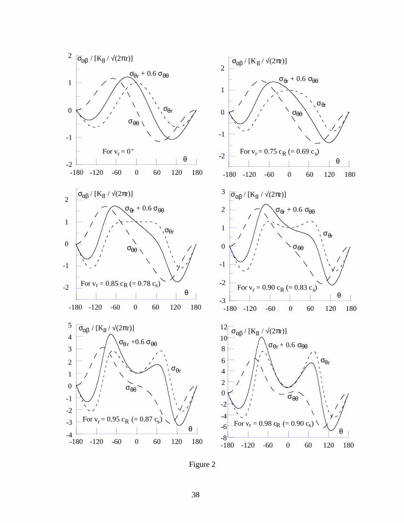
38

-2

-1

0

1

2

-180 -120 -60 0 60 120 180

θFor vr = 0+

σαβ / [KII / √(2πr)]

σθr

σθr + 0.6 σθθ

σθθ

-2

-1

0

1

2

-180 -120 -60 0 60 120 180

θFor vr = 0.75 cR (= 0.69 cs)

σαβ / [K II / √(2πr)]

σθr

σθr + 0.6 σθθ

σθθ

-2

-1

0

1

2

-180 -120 -60 0 60 120 180

θFor vr = 0.85 cR (= 0.78 cs)

σθr + 0.6 σθθ

σαβ / [KII / √(2πr)]

σθr

σθθ

-3

-2

-1

0

1

2

3

-180 -120 -60 0 60 120 180

θFor vr = 0.90 cR (= 0.83 cs)

σαβ / [KII / √(2πr)]

σθr

σθr + 0.6 σθθ

σθθ

-4

-3

-2

-1

0

1

2

3

4

5

-180 -120 -60 0 60 120 180

For vr = 0.95 cR (= 0.87 cs)θ

σθ r +0.6 σθθ

σθ r

σθθ

σαβ / [KII / √(2πr)]

-8

-6

-4

-2

0

2

4

6

8

10

12

-180 -120 -60 0 60 120 180

For vr = 0.98 cR (= 0.90 cs)θ

σαβ / [KII / √(2πr)]

σθr + 0.6 σθθ

σθr

σθθ

Figure 2

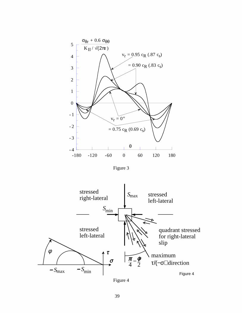
39

- 4

- 3

- 2

- 1

0

1

2

3

4

5

-180 -120 -60 0 60 120 180

θ

vr = 0+

= 0.75 cR (0.69 cs)

σθr + 0.6 σθθK II / √(2πr )

vr = 0.95 cR (.87 cs)

= 0.90 cR (.83 cs)

Figure 3

Smin

Smax

σ π φ4 2

−

φ

quadrant stressedfor right-lateral slip

stressedleft-lateral

stressedright-lateral

stressedleft-lateral

maximum τ/(−σ) direction

Figure 4

τ

−Smax −Smin

Figure 4

40

quadrant stressedfor right-lateral slip

maximum τ/(−σ) direction

Smax

Case with

−σyyo < −σ

xxo

(Low inclination

of Smax with fault)

quadrant stressedfor right-lateral slip

maximum τ/(−σ) direction

Smax

Case with

−σyyo > −σ

xxo

(High inclination

of Smax with fault)

Figure 5a

Figure 5b

ψ

ψ

Figure 5

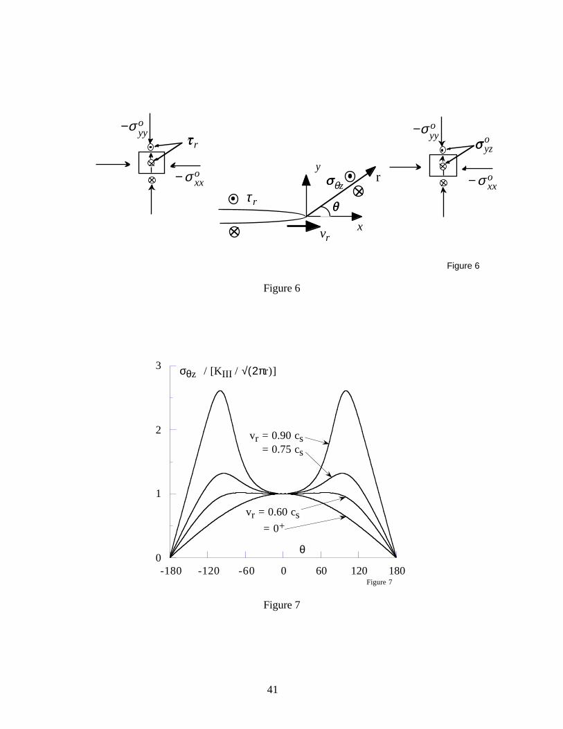
41

σθz

θ

r

vrx

y

Figure 6

τ r

−σyyo

−σ xxo

σ yzo

−σ yyo

−σ xxo

τ r

Figure 6

0

1

2

3

-180 -120 -60 0 60 120 180

θ

σθz / [KIII / √(2πr)]

vr = 0.90 cs = 0.75 cs

vr = 0.60 cs

= 0+

Figure 7

Figure 7

42

τ p

r

R

τ r

xvrFigure 8

( )σ σyx yz or τ

Figure 8

σ

τ r

τ σp p yyof= −

φpo= 30

Figure 9

τPeakStress

σxxo σyy

o

Figure 9

43

peak stress

a� )

P�

lanes of potential failures:

-1 0 1-1

0

1

x� /R�

0

y/R

0

Secondary faulting zone

- right lateral slip

Figure 10

b)

- left lateral slip

max Coulomb > 1)

Isolines of max Coulomb

Coulomb

max

Figure 10

44

−2 0 2−2

−1

0

1

2y/

Ro

vr/c

s =0

0.6

0.8

0.8

−2 0 2−2

−1

0

1

2v

r/c

s =0.7

0.6 0.6

0.8

0.8 1

−2 0 2−2

−1

0

1

2v

r/c

s =0.9

0.20.4

0.4

0.6

0.60.6

0.8

0.8

0.81

1

−2 0 2−2

−1

0

1

2

x/R0

y/R

o

vr/c

s =0

0.4

0.6

0.60.8

0.8

1

−2 0 2−2

−1

0

1

2

x/R0

vr/c

s =0.7

0.4

0.4

0.6

0.60.8

0.8

1

−2 0 2−2

−1

0

1

2

x/R0

vr/c

s =0.9

0.2 0

.4

0.4

0.4

0.6

0.6 0.6

0.8

0.8

0.8

1

1 1

σxxo /σ

yyo =0.8

Figure 13

Figure 11

a)

b)

σxxo /σ

yyo =2

Figure 11

45

r

Figure 12a

Figure 12b

σσ

φφ

xxo

yyo

p

p<

+−

≈1

11 7

2

2

sin

sin.

σσ

φφ

xxo

yyo

p

p>

+−

≈1

11 7

2

2

sin

sin.

vr

−σyyo

σ yxo

Initial stress

Initial stress

σ xxo

σ xxo

σ yyo

σ yyo

σ yxo

σ yxo

τ p

τ p

τ

τ

Peak stress

Peak stress

τ σp pf=−

τ σp pf=−

Figure 12

46

−2 0 2−2

−1

0

1

2

x/R0

y/R

o

τr / τ

p =0.2

0.2

0.2

0.2 0.2

0.2

0.4

0.4

0.4

0.40.4

0.4

0.4

0.6

0.6

0.6

0.6

0.6

0.6

0.6

0.8

0.8

0.8

0.8

0.8

11

1

1

−2 0 2−2

−1

0

1

2

x/R0

τr / τ

p =0.5

0.2

0.2

0.20.4

0.4

0.4

0.4 0.4

0.6 0.6

0.6

0.6

0.8

0.8

0.8

1

1−2 0 2

−2

−1

0

1

2

x/R0

τr / τ

p =0.8

0.6

0.8

0.8

0.8

0.8

0.8

1

11

vr/c

s=0.9 σ

xxo /σ

yyo =1

Figure 13

Figure 13

-0.5 0 0.5-0.5

0

0.5

Isolines of shear stress p

Damage zone ( p > 1)

Planes of maximum shear(potential secondary faults)

Figure 14x/R0

y/R0

Figure 14

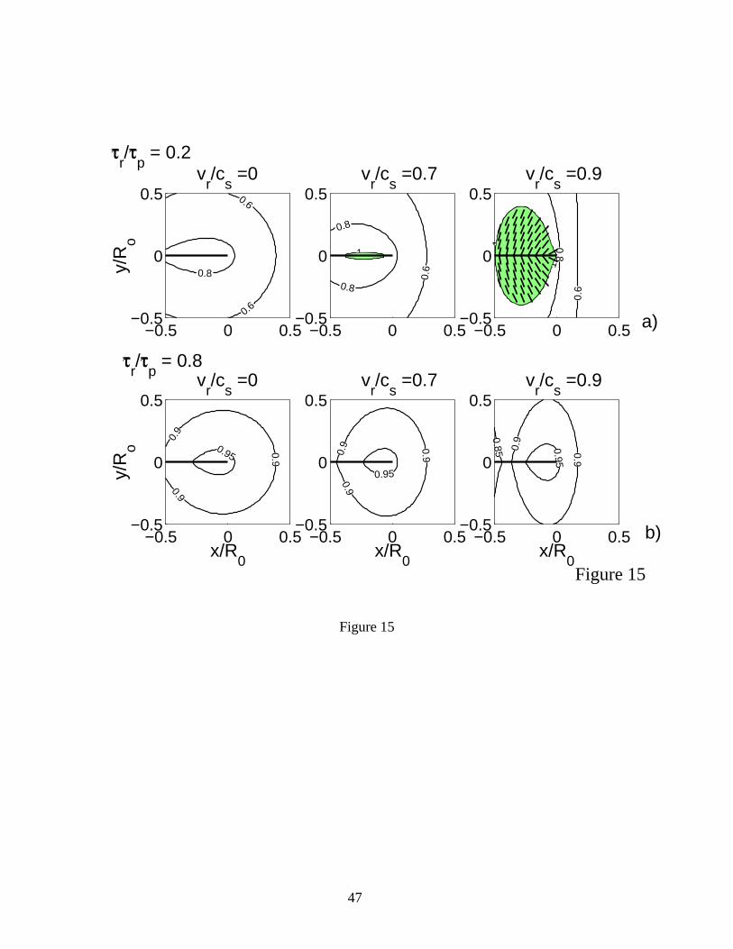
47

−0.5 0 0.5−0.5

0

0.5

y/R

o

vr/c

s =0

0.6

0.6

0.8

−0.5 0 0.5−0.5

0

0.5v

r/c

s =0.7

0.6

0.8

0.8

1

−0.5 0 0.5−0.5

0

0.5v

r/c

s =0.9

0.6

0.8

1

1

−0.5 0 0.5−0.5

0

0.5

x/R0

y/R

o

vr/c

s =0

0.9

0.9

0.9

0.95

−0.5 0 0.5−0.5

0

0.5

x/R0

vr/c

s =0.7

0.9 0.9

0.9

0.95

−0.5 0 0.5−0.5

0

0.5

x/R0

vr/c

s =0.9

0.85 0.9

0.9

0.95

τr/τ

p = 0.8

Figure 15

a)

b)

τr/τ

p = 0.2

Figure 15

48

a)b� )

c)d)

29˚

53˚

5 km

9 km

San

Fern

ando

197

1K

ettle

man

Hill

s 19

85

Lan

ders

199

2Im

peri

al V

alle

y 19

79

Sm

ax

Sm

ax

M=

6

M=

2M

=4

Sm

ax

Sm

ax

1 km

Johnson Val.Kickapoo

6 km

US-

Mex

ico

Impe

rial F

ault

N

Brawley F.Z.

Homestead Val.

rup

ture

propa

gatio

n

propagation

rupture

0 km 5 10

-10

km0

km10

km

Figu

re 1

6

400

m

0 m

Figure 16