Volterrafaces: Discriminant Analysis using Volterra Kernels ∗

Ritwik Kumar, Arunava Banerjee, Baba C. VemuriDepartment of Computer and Information Science and Engineering, University of Florida

{rkkumar,arunava,vemuri}@cise.ufl.edu

Abstract

In this paper we present a novel face classification sys-tem where we represent face images as a spatial arrange-ment of image patches, and seek a smooth non-linear func-tional mapping for the corresponding patches such that inthe range space, patches of the same face are close to oneanother, while patches from different faces are far apart,in L2 sense. We accomplish this using Volterra kernels,which can generate successively better approximations toany smooth non-linear functional. During learning, foreach set of corresponding patches we recover a Volterrakernel by minimizing a goodness functional defined overthe range space of the sought functional. We show thatfor our definition of the goodness functional, which mini-mizes the ratio between intra-class distances and inter-classdistances, the problem of generating Volterra approxima-tions, to any order, can be posed as a generalized eigen-value problem. During testing, each patch from the test im-age that is classified independently, casts a vote towardsimage classification and the class with the maximum votesis chosen as the winner. We demonstrate the effectivenessof the proposed technique in recognizing faces by extensiveexperiments on Yale, CMU PIE and Extended Yale B bench-mark face datasets and show that our technique consistentlyoutperforms the state-of-the-art in learning based face dis-crimination.

1. PrologueWorld events, specially in the last decade, have lead to

an increased interest in the field of biometrics based personidentification. Face recognition in particular, has attractedprolific research in the computer vision and pattern recogni-tion community. Even though impressive strides have beenmade towards providing an ultimate solution to this prob-lem, significant and interesting problems remain.

If we try to organize the epitome of literature present inthis field, a dichotomy of approaches emerges. The first

∗This work was supported in part by the UF Alumni Fellowship to RKand NIH grant NS46812 to BCV.

class of these tries to capture the physical processes of im-age formation under various scene parameter variations likeillumination (e.g. Generic ABRDF [3]), pose (e.g. Mor-phable Models[5]), expression(e.g. Geometry-Texture [16])etc. In contrast, the second class of approaches invokesmathematical and statistical tools to capture the structure ofthe oft-invisible relations among the numbers that make upthe face images. These techniques explore the intrinsic datageometry assuming images to be either vectors (e.g. Eigen-faces [17], Fisherfaces [4], Laplacianfaces [13], orthogo-nal Laplacianfaces (OLAP) [7], Locality Preserving Projec-tions [11], Kernel Locality Preserving Projections with SideInformation (KLPPSI) [2], MLASSO [18], Kernel RidgeRegression (KRR) [1]), or higher dimensional tensors (e.g.Tensor Subspace Analysis [12], 2-Dimensional Linear Dis-criminant Analysis [24], Orthogonal Rank One Tensor Pro-jection (ORO) [14], Tensor Average Neighborhood MarginMaximization (TANMM) [23], Correlation Tensor Analysis(CTA) [10], Spectral Regression [6], Regularized Discrimi-nant Analysis [6], Smooth LDA [8]).

A major advantage of the techniques in the first classcomes from their being generative in nature. This propertyallows these methods to accomplish tasks like face relight-ing (e.g. [3]) or novel pose generation or complete 3D im-age reconstruction (e.g. [5]) in addition to recognition. Atthe same time, methods in the first class tend to demandmore side information from the data as compared to thesecond class of methods (e.g. [3] requires illumination di-rection for the training set, [5] requires facial feature pointsfor initialization etc). The second class of methods are ina sense more versatile as they can be seamlessly applied toa variety of different image sets without any significant re-quirement of side information.

The method that we propose in this paper loosely fallsinto the second category of techniques. We seek a mappingof face image patches such that in the range space, discrimi-nation among different classes is easier. We choose Volterrakernels to accomplish this because it allows us to system-atically build progressively better approximations to sucha mapping. Furthermore, Volterra kernels can be learnt ina data driven fashion which relieves us from being predis-

150978-1-4244-3991-1/09/$25.00 ©2009 IEEE

Figure 1. Structure of A1i and A2

i for an image of size 5× 5 and kernel of size 3× 3. In the first row, 9 neighborhoods of the image Ii arehighlighted. For first order approximation, each of of these neighborhoods become a row in A1

i . For the second order case, we take all thesecond order combinations of pixel values in each neighborhood and use them as the first 81 (b4) elements of a row in A2

i . The remaining9 (b2) elements are simply the pixel values. Rows are numbered to show which neighborhood they correspond to.

posed towards any fixed kernel form (e.g. Gaussian, RadialBasis Function etc). The face images in the range space arecalled Volterrafaces in this paper.

2. Volterra Kernel Approximations

From signal processing theory we know that a lineartranslation invariant (LTI) functional = : H → H, whichmaps the function x(t) to the function y(t), can be com-pletely described by a function h(t) as

=(x(t)) = y(t) = x(t)⊗h(t) =∫ ∞−∞

h(τ)x(t−τ)dτ. (1)

Volterra theory generalizes this concept and states that anynon-linear translation invariant functional ℵ : H → H,which maps the function x(t) to the function y(t), can bedescribed by a sequence of functions hn(·) as

=(x(t)) = y(t) =∞∑

n=1

yn(t) (2)

where yn(t) =∫ ∞−∞· · ·

∫ ∞−∞

hn(τ1, . . . , τn)x(t−τ1) . . . x(t−τn)dτ1 · · · dτn(3)

Here hn(τ1, . . . , τn) are called the Volterra Kernels of thefunctional. It must be noted that the above equation can beseamlessly generalized to 2 dimensional functions, I(u, v),which for instance, can be images. It should be noted thateq. (1) is just a special case of the more general eq. (3) ifthe first order terms are the only ones taken into account.

Since we are interested in computing using this theory,we would be using the following discrete form of eq. (3).

yn(m) =∞∑

q1=−∞· · ·

∞∑qn=−∞

hn(q1, . . . , qn)x(m− q1) . . . x(m− qn).

(4)The infinite series form in eq. (4) does not lend itself wellfor practical implementations. Further, for a given applica-tion, only the first few terms may give the desired approxi-mation of the functional. Thus, we need a truncated form ofthe Volterra series, which is denoted in this paper by

=p(x(m)) =p∑

n=1

yn(m) = x(m)⊗p h(m) (5)

where p denotes the maximal order of the terms taken intoaccount for the approximation. Note that in this truncatedVolterra series representation, h(m) is a placeholder for allthe different orders of the kernels.

In general, given a set of input functions I, we are in-terested in finding a functional ℵ, such that ℵ(I) has somedesired property. This desired property can be captured bydefining a goodness functional on the range space of ℵ. Incases when the explicit equation relating the input set I toℵ(I) is known, various techniques like the harmonic inputmethod, direct expansion etc. ([9]) can be used to com-pute kernels of the unknown functional. In the absence ofsuch an explicit relation, we propose that the Volterra ker-nels be learnt from the data using the goodness functional.The translation invariance property of the Volterra kernelsensures that if the images are translated by a fixed amountin the domain, the mapped images are also translated bythe same amount, and hence the Volterra kernel mapping isstable.

In this framework, the problem of pattern classificationcan be posed as follows. Given a set of input data I = {gi}

151

where i = 1 . . . N , a set of classes C = {ck} wherek = 1 . . .K, and a mapping which associates each gi toa class ck, find a functional such that in the range space,the data ℵ(I) is easily classifiable. Here the goodness func-tional could be a measure of the separability of classes inthe range space. Once the Volterra kernels have been deter-mined, a new data point can be classified using the learntfunctional. ℵ(I) can be approximated to an appropriate ac-curacy based on computational efficiency and the classifica-tion accuracy constraints.

3. Kernel computation as Generalized Eigen-value problem

For the specific task of image classification, we definethe problem as follows. Given a set of input images (2Dfunctions) I, a training set, where each image belongs to aparticular class ck ∈ C, compute the Volterra kernels forthe unknown functional N which map the images in sucha manner that the goodness functional O is minimized inthe range space of N . Functional O measures the depar-ture from the complete separability of the data in the rangespace. In this paper we seek a functional N that maps allthe images from the same class in a manner such that theintraclass L2 distance is minimized while the interclass L2

distance is maximized. Once N has been determined, anew image can be classified using any of the methods likethe Nearest Centroid Classifier, Nearest Neighbor Classi-fiers etc. in the mapped space. With this observation, wedefine the goodness functional O as,

O(I) =

∑ck∈C

∑i,j∈ck

‖N (Ii)−N (Ij)‖2∑ck∈C

∑m∈ck,n/∈ck

‖N (Im)−N (In)‖2(6)

where the numerator measures the aggregate intraclass dis-tance for all the classes and the denominator measures theaggregate distance of class ck from all other classes in C.Equation (6) can be further expanded as

Ok(I) =

∑ck∈C

∑i,j∈ck

‖Ii ⊗p K − Ij ⊗p K‖2∑ck∈C

∑m∈ck,n/∈ck

‖In ⊗p K − Im ⊗p K‖2

(7)where K, like h(t) in eq. (5), is a placeholder for all thedifferent orders of the convolution kernels.

At this juncture we make the linear nature of convolutionexplicit by converting the convolution operation to multi-plication. This conversion to an explicit linear transforma-tional form can be done in many ways, but as the convolu-tion kernel is the unknown in our setup, we wish to keep itas a vector and thus we transform the image Ii into a newrepresentation Ap

i such that

Figure 2. Training images from each class are stacked up and di-vided into equal sized patches. Corresponding patches from eachclass are then used to learn Volterra kernels by minimizing intra-class distance over interclass distance. We end up with one Volerrakernel per group of spatially corresponding patches.

Ii ⊗p K = Api ·K (8)

whereK is the vectorized form of the 2D masks representedby K.

The exact form of Api depends on the order of the convo-

lutions p. In Section 5 we have presented results for up tothe second order approximations and thus the structure ofAp

i is explained for only up to second order, but it should benoted that the recognition framework using volterra kernelsthat we propose is very general and the structure of Ap

i forany order can be analogously derived.

3.1. First Order Approximation

For an image Ii of size m × n pixels and a first orderkernel K1 of size b × b, the transformed matrix Ap

i has di-mensions mn × b2. It is built by taking neighborhoods ofb × b dimensions at each pixel in Ii, vectorizing and thenstacking them one on top of the other. This procedure is il-lustrated for an image of size 5× 5 and kernel of size 3× 3in Figure 1. Border pixels can be ignored or taken into ac-count during convolution by padding the image with zeroswithout affecting the performance significantly.

Substituting the above defined representation for convo-lution in eq. (7), we obtain

O(I) =

∑ck∈C

∑i,j∈ck

‖Api ·K1 −Ap

j ·K1‖2∑

ck∈C∑

m∈ck,n/∈ck‖Ap

n ·K1 −Ami ·K1‖

2 .

(9)This can be written as

O(I) =K

T

1 SWK1

KT

1 SBK1

(10)

where SW =∑

ck∈C∑

i,j∈ck(Ap

i −Apj )

T (Api −A

pj ) and

SB =∑

ck∈C∑

m∈ck,n/∈ck(Ap

i −Apj )

T (Api −A

pj ).

152

Here SW and SB are symmetric matrices of dimensionsb2 × b2. Seeking the minimum of eq. (10) leads to solvingthe generalized eigenvalue problem and thus the minimumof O(I) is given by the minimum eigenvalue of SB

−1SW

and it is attained when K1 equals the corresponding eigen-vector.

3.2. Second Order Approximation

The second order approximation of the sought functionalcontains two terms

y(m) =∞∑

q1=−∞h1(q1)x(m− q1) +

∞∑q1=−∞

∞∑q2=−∞

h2(q1, q2)x(m− q1)x(m− q2)

(11)

The first term in eq. (11) corresponds to a weighted sumof the first order terms, x(m − q1), while the second termcorresponds to a weighted sum of the second order terms,x(m − q1)x(m − q2). For an image Ii of size m × n pix-els and kernels of size b × b, the transformed matrix A2

i

for the second order approximation in eq. (8) has dimen-sions mn × (b4 + b2) and the kernel vector that multipliesit, K2, has dimensions (b4 + b2)× 1. A2

i is built by takinga neighborhood of size b × b at each pixel in Ii, generat-ing all second degree combinations from the neighborhood,vectorizing them, concatenating the first degree terms andthen stacking them one on top of the other. K2 is formedby concatenating vectorized second and first order kernels.The structure of A2

i for a 5 × 5 image and 3 × 3 kernelsis illustrated in Figure 1. It must noted that the problem isstill linear in the variables being solved for and in fact byuse of this formulation we have ensured that regardless ofthe order of the approximation, the problem is linear in thecoefficients of the Volterra convolution kernels.

With this definition of A2i we proceed like the first or-

der approximation to obtain analogous equations (9) and(10) with the difference being that the matrices SB andSW now have dimensions (b4 + b2) × (b4 + b2). Herewe must point out an important modification to the struc-ture of A2

i which allows us to reduce the size of the matri-ces. The second order convolution kernels in the Volterraseries are required to be symmetrical ([9]) and this symme-try also manifests itself into the structure of A2

i . By allow-ing only unique entries in A2

i we can reduce the dimensionsof A2

i to mn × b4+3b2

2 and the dimensions of the matricesSB and SW to b4+3b2

2 × b4+3b2

2 . Now as in the first orderapproximation, the minimum ofOk(I) is given by the mini-mum eigenvalue of SB

−1SW, which it is attained whenK2

equals the corresponding eigenvector.

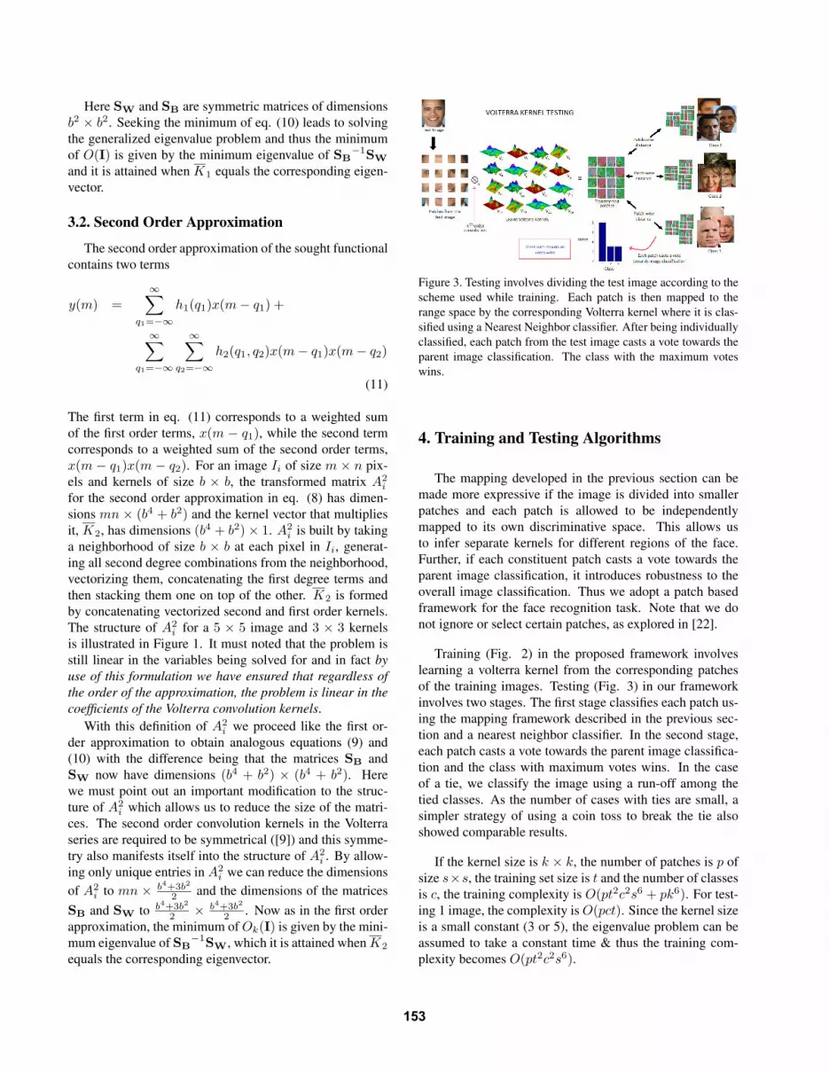
Figure 3. Testing involves dividing the test image according to thescheme used while training. Each patch is then mapped to therange space by the corresponding Volterra kernel where it is clas-sified using a Nearest Neighbor classifier. After being individuallyclassified, each patch from the test image casts a vote towards theparent image classification. The class with the maximum voteswins.

4. Training and Testing Algorithms

The mapping developed in the previous section can bemade more expressive if the image is divided into smallerpatches and each patch is allowed to be independentlymapped to its own discriminative space. This allows usto infer separate kernels for different regions of the face.Further, if each constituent patch casts a vote towards theparent image classification, it introduces robustness to theoverall image classification. Thus we adopt a patch basedframework for the face recognition task. Note that we donot ignore or select certain patches, as explored in [22].

Training (Fig. 2) in the proposed framework involveslearning a volterra kernel from the corresponding patchesof the training images. Testing (Fig. 3) in our frameworkinvolves two stages. The first stage classifies each patch us-ing the mapping framework described in the previous sec-tion and a nearest neighbor classifier. In the second stage,each patch casts a vote towards the parent image classifica-tion and the class with maximum votes wins. In the caseof a tie, we classify the image using a run-off among thetied classes. As the number of cases with ties are small, asimpler strategy of using a coin toss to break the tie alsoshowed comparable results.

If the kernel size is k × k, the number of patches is p ofsize s×s, the training set size is t and the number of classesis c, the training complexity is O(pt2c2s6 + pk6). For test-ing 1 image, the complexity isO(pct). Since the kernel sizeis a small constant (3 or 5), the eigenvalue problem can beassumed to take a constant time & thus the training com-plexity becomes O(pt2c2s6).

153

Method Yale A CMU PIE Ext. Yale B2008 CVPR, An et al. (KLPPSI) [2] - 5 10 20 30 5 10 20 302008 CVPR, Pham et al. (MLASSO) [18] - 2 3 4 2 3 42008 CVPR, Shan et al. (UVF) [20] 2 - 8 - -2008 TIP, Fu et al. (CTA) [10] - 5 10 15 20 5 10 20 302008 TIP, Fu et al. (Lap,Eig,Fis) [10] - - 5 10 20 302007 CVPR, An et al. (KRR) [1] - 5 10 20 30 5 10 20 302007 CVPR, Hua et al. (ORO) [14] 5 30 202007 CVPR, Cai et al. (S-LDA) [8] 2 3 4 5 - -2007 CVPR, Wang et al. (TANMM) [23] 2 3 4 5 10 20 -2007 ICCV, Cai et al. (SR, RDA) [6] - 30 40 10 20 30 402006 TIP, Cai et al. (OLAP) [7] 2 3 4 5 5 10 20 30 -2006 TIP, Cai et al. (Lap,Eig,Fis) [7] 2 3 4 5 5 10 20 30 -

Table 1. State-of-the-art methods with which we compare our tech-nique, along with the training set sizes used in their experiments.

4.1. Parameter Selection

Like any other learning algorithm, there are parametersthat need to be set before using this method. But unlikemost state-of-the-art algorithms where parameters are cho-sen from a large discrete or continuously varying domain(e.g. initialization and λ in [18], parameter α ∈ [0, 1] in [8],dimensionality D in [20], reduced dimensionality in TSA[12], 2D-LDA [24] , energy threshold in [19] etc.), Volterradiscriminant analysis has a smaller discrete set of param-eter choices. We use one of the widely used ([8],[1]) andaccepted methods, cross validation, for parameter selection.

Foremost is the selection of the patch size, and for this,starting with the whole face image we define a quad-tree ofsub-images. We progressively go down the tree stoppingat the level beyond which there is no improvement in therecognition rates as computed using cross validation. Em-pirically we found that a patch size of 8× 8 pixels providesthe best results in all cases. Next, we allow patches to beoverlapping or non-overlapping. The Volterra kernel sizecan be of size 3 × 3 or 5 × 5 pixels (anything bigger thanthis severely over-fits a patch of size 8×8). Lastly, the orderof the kernel can be quadratic or linear.

In this paper we have presented results for both quadraticand linear kernels. The rest of the parameters were set usinga 20-fold leave-one-out cross validation on the training set.It can be noted from the results presented in the next sectionthat the best parameter configuration is fairly consistent notonly within a particular database but also across databases.

5. Experiments

In order to evaluate our technique and compare it withexisting state-of-the-art methods in learning based facerecognition, we have identified 11 recent (Table 1) pub-lications which present the best results on the benchmarkdatabases using very similar (to that in [7]) experimentalsetups. All of these are embedding methods mentioned inthe prologue with the exception of [20] which builds on theconcept of Universal Visual Features (UVF). In our study,

we present results on Yale A, CMU PIE and Extended YaleB benchmark face databases partly because they are someof the most popular databases which makes a comparativestudy easy. In addition to the recent methods we also pro-vide comparisons with the traditional baseline methods -Eigenfaces, Fisherfaces and Laplacianfaces. Table. 1 liststhese methods along with the number of training imagesused by them on the above mentioned databases in theirexperiments. We have presented our results for the wholerange of training set sizes so that comparisons with a maxi-mum number of techniques can be made.

For the Yale A 1 face database we used 11 images eachof the 15 individuals with a total of 165 images. For theCMU PIE database ([21]) we used all 170 images (ex-cept a few corrupted images) from 5 near frontal poses(C05,C07,C09,C27,C29) for each of the 68 subjects. Forthe Extended Yale B database ([15]) we used 64 (except fora few corrupted images) images each (frontal pose) of 38individuals present in the database. Note that the methodsin Table. 1 used the same subset of images. We obtained thedata from the website of the authors of [8] 2. These imageswere manually aligned (two eyes were aligned at the sameposition) and cropped to extract faces, with 256 gray valuelevels per pixel.

The results (average recognition error rates) on the YaleA, the CMU PIE and the Extended Yale B databases arepresented in Table. 1(a), Table. 1(b) and Table. 1(c), re-spectively. Rows titled Train Set Size indicate the numberof training images used and the rows below them list therates reported by various state-of-the-art and our method(Volterrafaces). Each experiment was repeated 10 times for10 random choices of the training set. All images other thanthe training set were used for testing. Specific experimentalsetup used for Volterrafaces is mentioned below each ta-ble. We have reported results with both linear and quadraticmasks for the sake of completeness. Best results for a par-ticular training set size are highlighted in bold.

5.1. Discussion

It can be noted that our proposed method (Volterrafaces)consistently outperforms the state-of-the-art and traditionalmethods on all the three benchmark datasets. On allthe three databases, linear masks outperform the quadraticmasks but in most cases quadratic masks also provided bet-ter performance than the existing methods. For the compet-ing methods we have reported the error rates as mentionedin the original publications (listed next to the method namesin the tables). Since we want to present only the best resultsreported by the competing methods, some of the entries inthe tables are left empty because no results for those train-ing set sizes were reported in the original publications.

1http://cvc.yale.edu/projects/yalefaces/yalefaces.html2http://www.cs.uiuc.edu/homes/dengcai2/Data/data.html

154

(a) Yale ATrain Set Size 2 3 4 5S-LDA [8] 42.4 27.7 22.2 18.3S-LDA [8] (updated) 37.5 25.5 19.3 14.7UVF [20] 27.11 17.38 11.71 8.16TANMM [23] 44.69 29.57 18.44 -OLAP [7] 44.3 29.9 22.7 17.9Eigenfaces [7] 56.5 51.1 47.8 45.2Fisherfaces [7] 54.3 35.5 27.3 22.5Laplacianfaces [7] 43.5 31.5 25.4 21.7Volterrafaces (Linear) 15.70 12.33 9.47 6.11Volterrafaces (Quad) 22.15 13.36 15.78 10.19

Train Set Size 6 7 8 9S-LDA [8] (updated) 12.3 10.3 8.7 -UVF [20] 6.27 5.07 3.82 -Volterrafaces (Linear) 5.78 3.96 2.61 1.43Volterrafaces (Quad) 10.04 9.66 9.49 8.74

(b) CMU PIETrain Set Size 5 10 20 30KLPPSI [2] 27.88 12.32 5.48 3.62KRR [1] 26.4 13.1 5.97 4.02ORO [14] - - - 6.4TANMM [23] 26.98 17.22 5.68 -SR [6] - - - 6.1OLAP [7] 21.4 11.4 6.51 4.83Eigenfaces [7] 69.9 55.7 38.1 27.9Fisherfaces [7] 31.5 22.4 15.4 7.77Laplacianfaces [7] 30.8 21.1 14.1 7.13Volterrafaces (Linear) 20.26 10.24 4.94 2.85Volterrafaces (Quad) 25.29 11.94 5.45 4.60

Train Set Size 2 3 4 40SR [6] - - - 5.2MLASSO [18] 54.0 43.0 34.0 -Volterrafaces (Linear) 43.0 36.30 23.98 2.37Volterrafaces (Quad) 50.48 39.66 32.67 3.04

(c) Extended Yale BTrain Set Size 5 10 20 30ORO [14] - - - 9.0SR [6] - 12.0 4.7 2.0RDA [6] - 11.6 4.2 1.8KLPPSI [2] 24.74 9.93 3.15 1.39KRR [1] 23.9 11.04 3.67 1.43CTA [10] 16.99 7.60 4.96 2.94Eigenfaces [10] 54.73 36.06 31.22 27.71Fisherfaces [10] 37.56 18.91 16.87 14.94Laplacianfaces [10] 34.08 18.03 30.26 20.20Volterrafaces (Linear) 6.35 2.67 0.90 0.42Volterrafaces (Quad) 13.0 3.98 1.27 0.58

Train Set Size 2 3 4 40MLASSO [18] 58.0 54.0 50.0 -SR [6] - - - 1.0RDA [6] - - - 0.9Volterrafaces (Linear) 26.23 18.23 9.33 0.34Volterrafaces (Quad) 40.81 20.47 14.42 0.43

Table 2. Yale A Training set size: 2-9, Linear kernel size: 5 × 5, Quadratic kernel size: 3 × 3, overlapping patches size: 8 × 8, imagessize: 64× 64. CMU PIE: Training set size: 2-9, Linear kernel size: 5× 5, Quadratic kernel size: 3× 3, overlapping patches size: 8× 8,images size: 32× 32. Extended Yale B, Training set size: 2-5, 5, 10, 20, 30 & 40 Linear kernel size: 3× 3, Quadratic kernel size: 3× 3,non-overlapping patches size: 8× 8, images size: 32× 32. For other methods, best results as reported in the respective papers are used.

6. Conclusion

We have introduced the use of Volterra kernel approxi-mations for image recognition functionals in this paper. Thekernel learning is driven by the training data, based on agoodness functional defined in the range space of the recog-nition functional. It is shown that for a goodness functionalthat tries to minimize intraclass distances while maximizinginterclass distances, the kernel computation reduces to thegeneralized eigenvalue problem which translates to a veryefficient computation of kernels for any order of approxi-mation of the functional. Effectiveness of this technique forface recognition is demonstrated by experiments on threebenchmark databases and the results are compared to tradi-tional as well as the state of the art techniques in discrim-inant analysis for faces. From the results presented in thispaper it can be concluded that Volterra kernel approxima-tions show great promise for applications in image recogni-tion tasks.

References[1] S. An, W. Liu, and S. Venkatesh. Face recognition using

kernel ridge regression. In CVPR, 2007.[2] S. An, W. Liu, and S. Venkatesh. Exploiting side information

in locality preserving projection. In CVPR, 2008.[3] A. Barmpoutis, R. Kumar, B. C. Vemuri, and A. Baner-

jee. Beyond the lambertian assumption: A generative modelfor apparent brdf fields of faces using anti-symmetric tensorsplines. CVPR, pages 1–6, 24 - 26 June 2008.

[4] P. N. Belhumeur, J. Hespanha, and D. J. Kriegman. Eigen-faces vs. fisherfaces: Recognition using class specific linearprojection. PAMI, 19(7):711–720, 1997.

[5] V. Blanz and T. Vetter. Face recognition based on fitting a 3dmorphable model. PAMI, 25(9):1063–1074, 2003.

[6] D. Cai, X. He, and J. Han. Spectral regression for efficientregularized subspace learning. In ICCV, 2007.

[7] D. Cai, X. He, J. Han, and H. J.Zhang. Orthogonal laplacian-faces for face recognition. TIP, 15(11), 2006.

[8] D. Cai, X. He, Y. Hu, J. Han, and T. Huang. Learning aspatially smooth subspace for face recognition. In CVPR,2007.

[9] J. A. Cherry. Introduction to volterra methods. DistortionAnalysis of Weakly Nonlinear Filters Using Volterra Series,1994.

[10] Y. Fu and T. S. Huang. Image classification using correlationtensor analysis. IEEE TIP, 17(2), 2008.

[11] X. He, D. Cai, and P. Niyogi. Locality preserving projec-tions. In NIPS, 2003.

[12] X. He, D. Cai, and P. Niyogi. Tensor subspace analysis. InNIPS, 2005.

[13] X. He, S. Yan, Y. Hu, P. Niyogi, and H. Zhang. Face recog-nition using laplacianfaces. IEEE PAMI, 27(3), 2005.

[14] G. Hua, P. Viola, and S. Drucker. Face recognition using dis-criminatively trained orthogonal rank one tensor projections.In CVPR, 2007.

[15] K. Lee, J. Ho, and D. J. Kriegman. Acquiring linear sub-spaces for face recognition under variable lighting. PAMI,27(5):684–698, 2005.

[16] X. Li, G. Mori, and H. Zhang. Expression-invariant facerecognition with expression classification. Third CanadianConference on Computer and Robot Vision, 2006.

[17] A. Pentland, B. Moghaddam, and T. Starner. View-based andmodular eigenfaces for face recognition. CVPR, 1994.

[18] D.-S. Pham and S. Venkatesh. Robust learning of discrimina-tive projection for multicategory classification on the stiefelmanifold. In CVPR, 2008.

[19] S. Rana, W. Liu, M. Lazarescu, and S. Venkatesh. Recog-nising faces in unseen modes: a tensor based approach. InCVPR, 2008.

[20] H. Shan and G. W. Cottrell. Looking around the backyardhelps to recognize faces and digits. In CVPR, 2008.

[21] T. Sim and T. Kanade. Combining models and exemplars forface recognition: An illuminating example. In CVPR Work-shop on Models versus Exemplars in Comp. Vision 2001.

[22] Y. Su, S. Shan, X. Chen, and W. Gao. Patch-based gaborfisher classifier for face recognition. In ICPR, 2006.

[23] F. Wang and C. Zhang. Feature extraction by maximizing theaverage neighborhood margin. In CVPR, 2007.

[24] J. Ye, R. Janardan, and Q. Li. Two-dimensional linear dis-criminant analysis. In NIPS, 2004.

155