Vine variety discrimination with airborne imaging

spectroscopy

M. Ferreiro-Armana, J. L. Alba-Castroa, S. Homayounib, J. P. da Costab and J.

Martın-Herreroa

aDept. de Teorıa do Sinal e Comunicacions, ETSET, Universidade de Vigo, E-36310, SpainbLAPS - UMR 5131 CNRS - Universite Bordeaux 1, F-33405 Talence, France ∗

ABSTRACT

We aim at the discrimination of varieties within a single plant species (Vitis vinifera) by means of airbornehyperspectral imagery collected using a CASI-2 sensor and supervised classification, both under constant andvarying within-scene illumination conditions. Varying illumination due to atmospheric conditions (such as clouds)and shadows cause different pixels belonging to the same class to present different spectral vectors, increasingthe within class variability and hindering classification. This is specially serious in precision applications suchas variety discrimination in precision agriculture, which depends on subtle spectral differences. In this study,we use machine learning techniques for supervised classification, and we also analyze the variability within andamong plots and within and among sites, in order to address the generalizability of the results.

Keywords: Vine variety discrimination, support vector machines, supervised classification, remote sensing,hyperspectral imagery

1. INTRODUCTION

The interest in the application of remote sensing to precision agriculture has been growing in the recent yearsthanks to recent advances in remote sensing devices. Airborne multispectral and hyperspectral imagery hasallowed a mapping of yield, soil properties, or diseases1–6 in the framework of precision viticulture. The vineyardcanopy has been accurately characterized recently by using affordable hyperspectral devices, including varietymapping. Though several studies have demonstrated the suitability of remotely sensed data for the discriminationof plant species,7–9 the capability of these remotely sensed hyperspectral data for grape variety mapping has notbeen given a big deal of attention.10–13 Grape variety discrimination is seen as a useful tool for vine growers todetect misplantings and to manage inner field species variability. Additionally, varietal discrimination enablesthe regional mapping of vine varieties, which can be used for planning and inventory purposes. For instance, inthe Bordeaux wine producing area in France, vine producer unions need tools to help in the certification of winegrowers. Varietal mapping is thus a valuable help in the certification of wine productions.

On the other hand, modern hyperspectral remote sensing devices allow images of natural scenes to be ac-quired with high radiometric, spatial, and spectral resolutions. This implies an enhanced resolving capability forvine variety discrimination within a given species13,14 but, however, these higher resolutions also imply a greaterinfluence of the context (atmosphere, illuminant, interferences) on the analytical results. Atmospheric influencehas been paid a great deal of attention since the early times of satellital remote sensing, with the developmentof detailed physical models (parametric and non parametric).15–17 Sensor calibration has received also a similar

∗This work has been cofinanced with ERDF funds through the Interreg IIIb “Atlantic Area” program within the PIMHAI project.

Further author information: (Corresponding author M.F.-A.)M.F.-A.: E-mail: mferreir@gts.tsc.uvigo.es, Telephone: +34 986 812155J.-L.A.-C.: E-mail: jalba@gts.tsc.uvigo.es, Telephone: +34 986 812680S.H.: E-mail: Saeid.Homayouni@laps.u-bordeaux1.fr

J.P.d.C.: E-mail: jean-pierre.dacosta@laps.ims-bordeaux.fr

J.M.-H.: E-mail: julio@gts.tsc.uvigo.es, Telephone: +34 986 812126

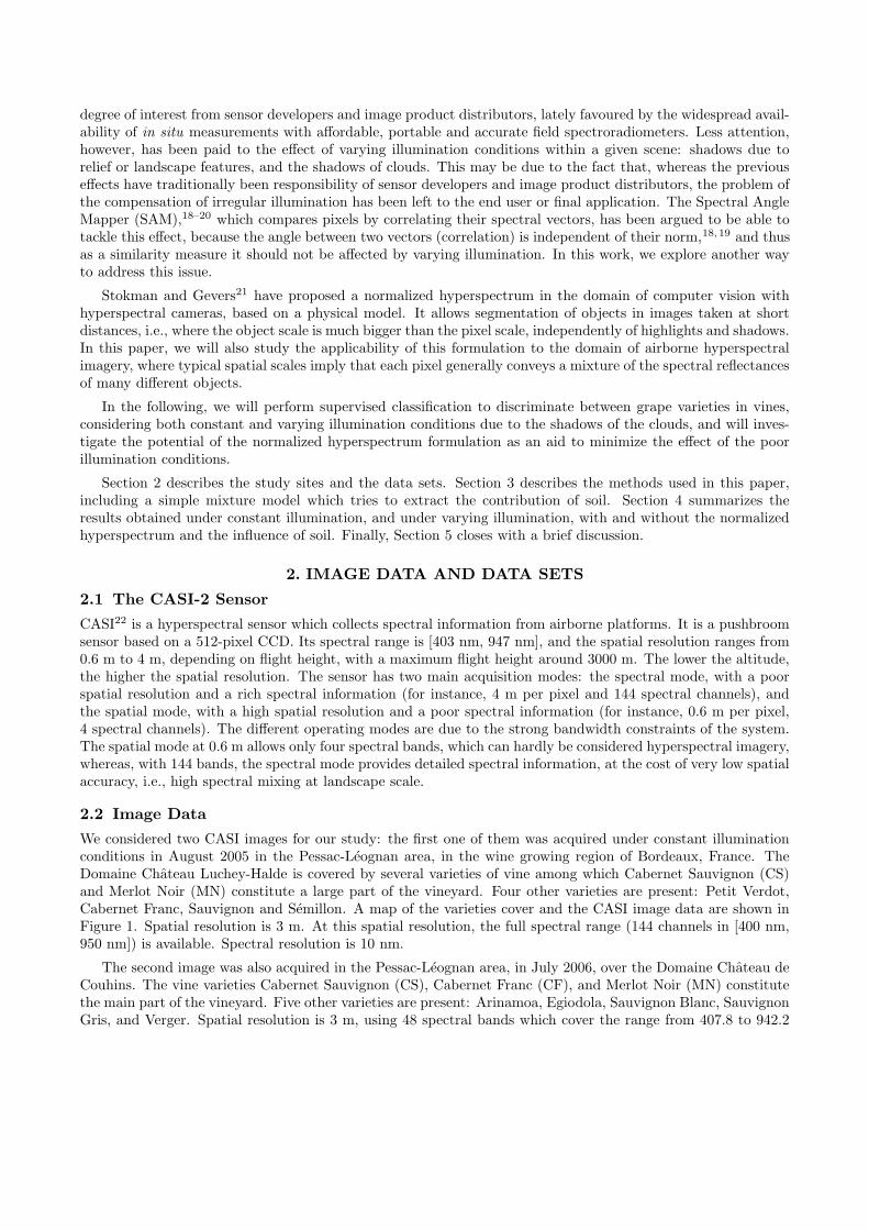
degree of interest from sensor developers and image product distributors, lately favoured by the widespread avail-ability of in situ measurements with affordable, portable and accurate field spectroradiometers. Less attention,however, has been paid to the effect of varying illumination conditions within a given scene: shadows due torelief or landscape features, and the shadows of clouds. This may be due to the fact that, whereas the previouseffects have traditionally been responsibility of sensor developers and image product distributors, the problem ofthe compensation of irregular illumination has been left to the end user or final application. The Spectral AngleMapper (SAM),18–20 which compares pixels by correlating their spectral vectors, has been argued to be able totackle this effect, because the angle between two vectors (correlation) is independent of their norm,18,19 and thusas a similarity measure it should not be affected by varying illumination. In this work, we explore another wayto address this issue.

Stokman and Gevers21 have proposed a normalized hyperspectrum in the domain of computer vision withhyperspectral cameras, based on a physical model. It allows segmentation of objects in images taken at shortdistances, i.e., where the object scale is much bigger than the pixel scale, independently of highlights and shadows.In this paper, we will also study the applicability of this formulation to the domain of airborne hyperspectralimagery, where typical spatial scales imply that each pixel generally conveys a mixture of the spectral reflectancesof many different objects.

In the following, we will perform supervised classification to discriminate between grape varieties in vines,considering both constant and varying illumination conditions due to the shadows of the clouds, and will inves-tigate the potential of the normalized hyperspectrum formulation as an aid to minimize the effect of the poorillumination conditions.

Section 2 describes the study sites and the data sets. Section 3 describes the methods used in this paper,including a simple mixture model which tries to extract the contribution of soil. Section 4 summarizes theresults obtained under constant illumination, and under varying illumination, with and without the normalizedhyperspectrum and the influence of soil. Finally, Section 5 closes with a brief discussion.

2. IMAGE DATA AND DATA SETS

2.1 The CASI-2 Sensor

CASI22 is a hyperspectral sensor which collects spectral information from airborne platforms. It is a pushbroomsensor based on a 512-pixel CCD. Its spectral range is [403 nm, 947 nm], and the spatial resolution ranges from0.6 m to 4 m, depending on flight height, with a maximum flight height around 3000 m. The lower the altitude,the higher the spatial resolution. The sensor has two main acquisition modes: the spectral mode, with a poorspatial resolution and a rich spectral information (for instance, 4 m per pixel and 144 spectral channels), andthe spatial mode, with a high spatial resolution and a poor spectral information (for instance, 0.6 m per pixel,4 spectral channels). The different operating modes are due to the strong bandwidth constraints of the system.The spatial mode at 0.6 m allows only four spectral bands, which can hardly be considered hyperspectral imagery,whereas, with 144 bands, the spectral mode provides detailed spectral information, at the cost of very low spatialaccuracy, i.e., high spectral mixing at landscape scale.

2.2 Image Data

We considered two CASI images for our study: the first one of them was acquired under constant illuminationconditions in August 2005 in the Pessac-Leognan area, in the wine growing region of Bordeaux, France. TheDomaine Chateau Luchey-Halde is covered by several varieties of vine among which Cabernet Sauvignon (CS)and Merlot Noir (MN) constitute a large part of the vineyard. Four other varieties are present: Petit Verdot,Cabernet Franc, Sauvignon and Semillon. A map of the varieties cover and the CASI image data are shown inFigure 1. Spatial resolution is 3 m. At this spatial resolution, the full spectral range (144 channels in [400 nm,950 nm]) is available. Spectral resolution is 10 nm.

The second image was also acquired in the Pessac-Leognan area, in July 2006, over the Domaine Chateau deCouhins. The vine varieties Cabernet Sauvignon (CS), Cabernet Franc (CF), and Merlot Noir (MN) constitutethe main part of the vineyard. Five other varieties are present: Arinamoa, Egiodola, Sauvignon Blanc, SauvignonGris, and Verger. Spatial resolution is 3 m, using 48 spectral bands which cover the range from 407.8 to 942.2

Figure 1. Domaine Chateau Luchey-Halde: CASI image data (left) and varieties cover (right).

nm. Spectral resolution is 6.3 nm. Figure 2 shows at the top a real colour image of the domain obtained fromthe CASI hyperspectral data, which is badly affected by cloud shadows. The corresponding variety map is shownat the bottom of the figure.

2.3 Data Sets

We built a series of data sets for testing the discriminability of the main aforementioned vine varieties in theCASI data by means of supervised classification, considering the different illumination conditions. In the case ofconstant illumination (Chateau Luchey-Halde), we discriminated between varieties CS and MN. For this purpose,we built two different data sets, each split into a training set and a testing set. Pixels within the MN and CSvarieties were selected in specific parcels. These two data sets were built to see whether the parcels where thetraining and testing pixels are picked from had or not a noticeable impact on the classification outcomes.

Tables 1 and 2 show the composition of each data set.

Table 1. Data set 1 for Chateau Luchey-Halde.

Class Training TestingMN 100

Plateau 2

400Conservatoire 2, Chenil 1, 2, Marroniers, Chenes 3a, 3b, 5

CS 100Essai PG E (left)

400Platanes, Plateau 1, Luchey 1, 4

Soil 50 200Trees 50 200

For the case of varying illumination (Chateau de Couhins), we tried to discriminate the three main varieties(CS, CF, and MN) by pairs: CS vs. CF, CS vs. MN, and CF vs. MN. For each pair, we tested the discriminationpotential among plots with different illumination conditions: in (“dark”) and out (“light”) of the cloud shadow.We also tested the discrimination in the pooled data. Thus, we generated three datasets for each variety (“dark”,“light”, and “joint”). Each of the sets was subsequently normalized according to the normalized hyperspectrumformulation of Stokman and Gevers21 and subjected to a simple unmixing strategy (see Section 3), in order togenerate the collection of train and test sets required for the comparisons. Table 3 lists the datasets, accordingto their illumination conditions. The labels refer to the plot codes in Figure 2.

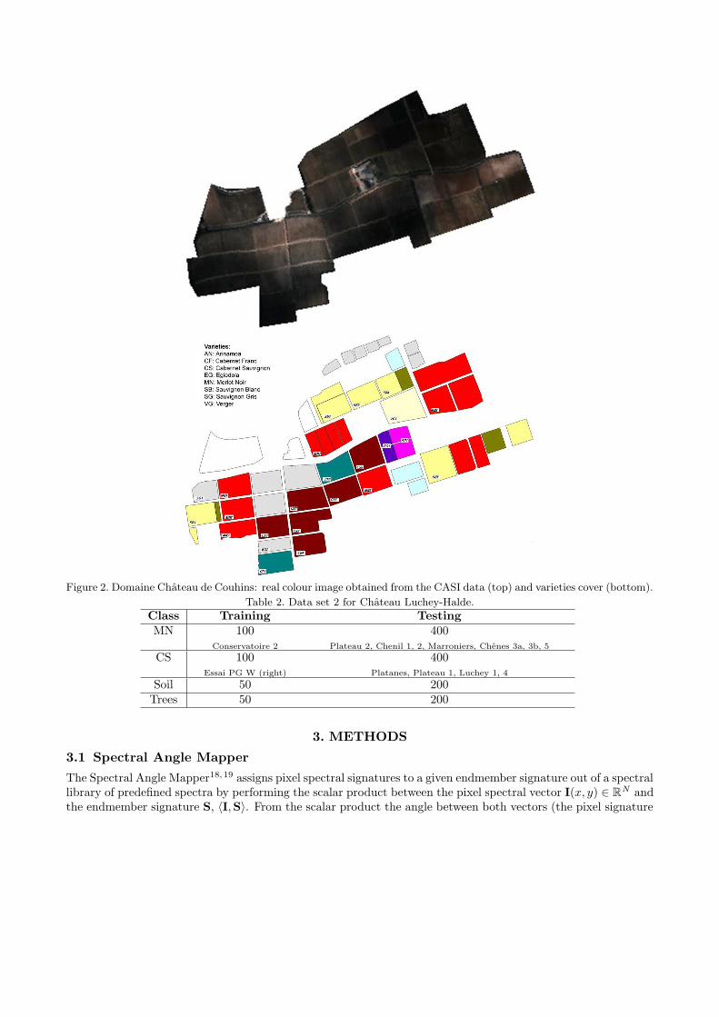
Figure 2. Domaine Chateau de Couhins: real colour image obtained from the CASI data (top) and varieties cover (bottom).

Table 2. Data set 2 for Chateau Luchey-Halde.

Class Training TestingMN 100

Conservatoire 2

400Plateau 2, Chenil 1, 2, Marroniers, Chenes 3a, 3b, 5

CS 100Essai PG W (right)

400Platanes, Plateau 1, Luchey 1, 4

Soil 50 200Trees 50 200

3. METHODS

3.1 Spectral Angle Mapper

The Spectral Angle Mapper18,19 assigns pixel spectral signatures to a given endmember signature out of a spectrallibrary of predefined spectra by performing the scalar product between the pixel spectral vector I(x, y) ∈ R

N andthe endmember signature S, 〈I,S〉. From the scalar product the angle between both vectors (the pixel signature

Table 3. Selected plots for each variety according to the illumination conditions, and joint datasets, without regard as tothe illumination. The size of each dataset is shown.

Illumination Variety Plot code Train TestLight CF CF2 68 61

MN MN1 81 67CS CS2 88 72

Dark CF CF1 61 46MN MN4 103 92

MN5 70 58CS CS5 86 81

Joint CF 129 107MN 463 397CS 490 433

and the endmember spectrum) is obtained,

θ = arccos

(

〈I,S〉

‖I‖ ‖S‖

)

, (1)

where ‖·‖ denotes the Euclidean norm. The smaller the angle, the closer (the more similar) the pixel is consideredto be to the endmember’s class. SAM assumes that hyperspectral image data have been reduced to “apparentreflectance”, with all dark current and path radiance biases removed. It has been argued that the independence ofthe spectral angle from the vector norm ensures independence of the similarity measure from varying illuminationconditions, an assumption that is usually taken for granted in the studies using SAM.

3.2 Hyperspectrum Normalization

According to Stokman and Gevers,21 given a hyperspectral image consisting of N image channels {Ii}Ni=1, we

can model each image channel as the output of a narrow filter with spectral response hi(λ) and input the albedoand Fresnel reflectances ra(λ) and rf(λ), of a surface patch viewed with an angle α, illuminated by a spectralpower distribution e(λ) with incidence angle ρ, and subjected to the geometric influence of the patch, ga(ρ) andgf(ρ, α),

Ii =

∫

λ

hi(λ)e(λ)[ga(ρ)ra(λ) + gf(ρ, α)rf(λ)]dλ. (2)

Matte objects only show albedo reflection, whereas the Fresnel reflectance present in shiny objects can beassumed to be independent of the wavelength in the range of interest, rf(λ) = rf , according to the neutralinterface reflection model.

The normalized hyperspectrum for albedo reflectance is defined as

Ii =Ii

∑N

j=1 Ij

, (3)

which can be easily shown to be invariant of the geometry (shading and shape) for matte objects. If we letki =

∫

λhi(λ)e(λ)ra(λ)dλ, then, assuming rf(λ) = 0,

Ii =ga(ρ)ki

∑N

j=1 ga(ρ)kj

=ki

∑N

j=1 kj

. (4)

In airborne imaging, Fresnel reflectance of shiny surfaces such as water can be decreased below significance bysuitable selection of flight paths with respect to solar incidence. In any case, assuming radiometrically correcteddata and sufficiently narrow bands (hyperspectral image), if we compute

Ii = Ii − minj=1,...N

{Ij}, (5)

we obtain a spectrum invariant to highlights.

Just let Ii = ga(ρ)ra(λi) + gf(ρ, α)rf = ga(ρ)ki + gf(ρ, α)rf , then

Ii = ga(ρ)ki + gf(ρ, α)rf − minj

{ga(ρ)kj + gf(ρ, α)rf}

= ga(ρ)ki + gf(ρ, α)rf − (ga(ρ)kmin + gf(ρ, α)rf)

= ga(ρ)(ki − kmin). (6)

By combining the two steps, we get the normalized hyperspectrum

Ii =Ii − min{Ij}

∑N

k=1 Ik − N min{Ij}. (7)

3.3 A Simple Spectral Unmixing Model

Given the moderate resolution we are using with respect to plant size in the Couhins image (3 metres), andthe scarcity of the canopy of prunned quality vines, soil backscatter is likely to have a significant impact onthe spectral signature of the image pixels. In order to attenuate this contribution, we implemented a simplespectral unmixing strategy, aiming at reducing as much as possible the fraction of the typical soils signature inthe spectral vectors of the datasets.

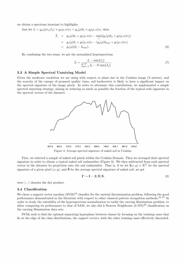
Figure 3. Average spectral signature of naked soil in Couhins.

First, we selected a sample of naked soil pixels within the Couhins Domain. Then we averaged their spectralsignature in order to obtain a typical naked soil endmember (Figure 3). We then subtracted from each spectralvector in the datasets its projection onto the soil endmember. That is, if we let I(x, y) ∈ R

N be the spectral

signature of a given pixel (x, y), and S be the average spectral signature of naked soil, we get

I∗ = I − 〈I, S〉 S, (8)

were 〈·, ·〉 denotes the dot product.

3.4 Classification

We chose a support vector machine (SVM)23 classifier for the varietal discrimination problem, following the goodperformance demonstrated in the literature with respect to other classical pattern recognition methods.24–27 Inorder to study the suitability of the hyperspectrum normalization to tackle the varying illumination problem, toallow comparing its performance to that of SAM, we also did k-Nearest Neighbours (k-NN)28 classification onthe varying illumination data sets.

SVMs seek to find the optimal separating hyperplane between classes by focusing on the training cases thatlie at the edge of the class distributions, the support vectors, with the other training cases effectively discarded.

Many hyperplanes could be fitted to separate the classes, but there is only one optimal separating hyperplane,that minimizes the separating margin, which is expected to generalize well in comparison to other hyperplanes.

The k-NN classification rule is a simple technique for non-parametric supervised classification. Given theknowledge of n prototype patterns and their correct classification into several classes, it assigns an unclassifiedpattern to the class that is most heavily represented among its k nearest neighbours in the pattern space.

4. RESULTS

This section presents the variety discrimination results obtained under constant illumination conditions, andunder varying illumination conditions. In this last case, we present the results obtained with the original andthe normalized data, and with and without the contribution of soil. For constant illumination, we used SVMwith a Gaussian kernel (C = 100 and γ = 0.1), while for varying illumination we used 5-NN and the same SVMas in the constant illumination case.

To quantify the goodness of the classification, we computed the overall accuracy (OA) and the κ statistic.29

κ measures how far from chance the results are, with a value in [0, 1]: when there is no agreement other thanthat which would be expected by chance, κ is zero. When there is total agreement, κ is one.

4.1 Constant Illumination Conditions

As we saw in Section 2, in this case we discriminated between the vine varieties CS and MN. Table 4 shows theclassification outcomes obtained from data sets 1 and 2 (Tables 1 and 2, respectively).

Table 4. Classification results obtained under constant illumination conditions using the SVM classifier.

Data Set κ (%) OA (%)1 86.8 90.52 83.6 88.2

Figure 4 shows the thematic maps obtained for the whole image.

Figure 4. Thematic maps for the Luchey image over data set 1 (left), and over data set 2 (right).

4.2 Varying Illumination Conditions

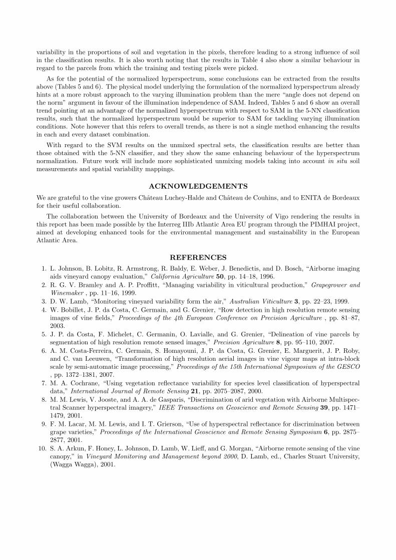
We considered in this experiment three varieties: CS, CF, and MN, following the strategy presented in Section2. Table 5 shows the results obtained using 5-NN with SAM on the original data, 5-NN with Euclidean distanceon the normalized data, SVM on the original data, and SVM on the normalized data, for the complete (notunmixed) spectra. Table 6 shows the same for the unmixed spectra.

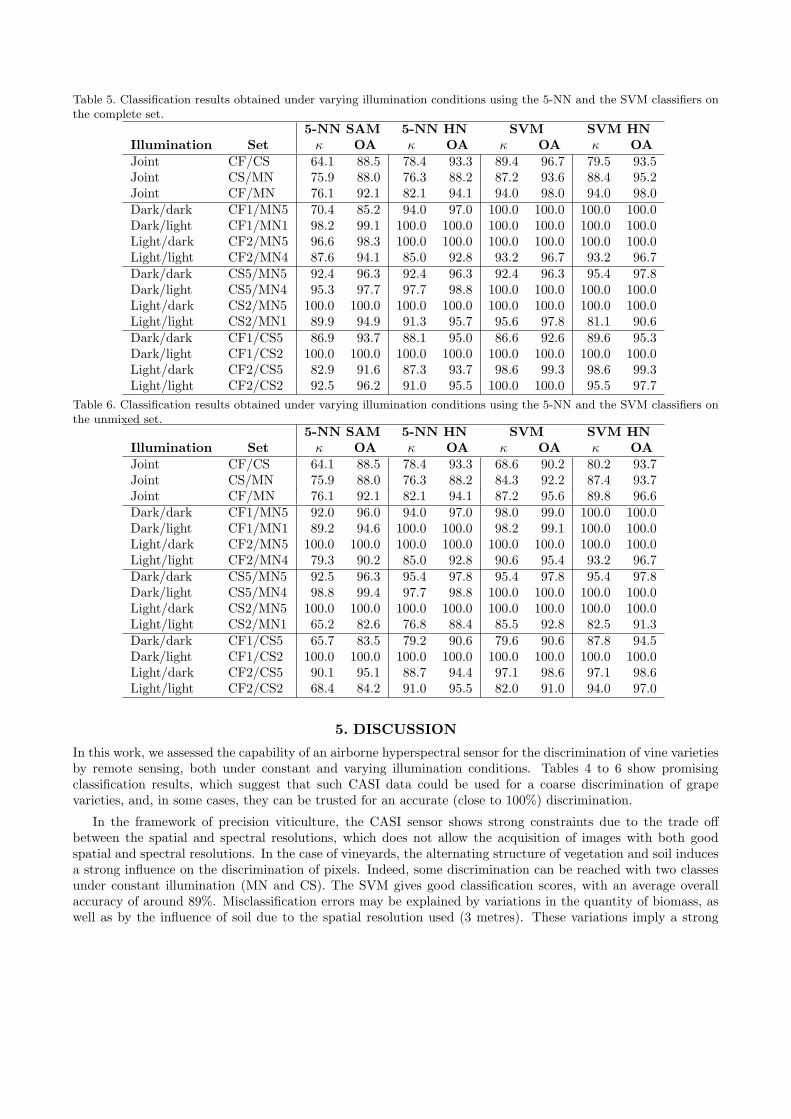
Table 5. Classification results obtained under varying illumination conditions using the 5-NN and the SVM classifiers onthe complete set.

5-NN SAM 5-NN HN SVM SVM HNIllumination Set κ OA κ OA κ OA κ OAJoint CF/CS 64.1 88.5 78.4 93.3 89.4 96.7 79.5 93.5Joint CS/MN 75.9 88.0 76.3 88.2 87.2 93.6 88.4 95.2Joint CF/MN 76.1 92.1 82.1 94.1 94.0 98.0 94.0 98.0Dark/dark CF1/MN5 70.4 85.2 94.0 97.0 100.0 100.0 100.0 100.0Dark/light CF1/MN1 98.2 99.1 100.0 100.0 100.0 100.0 100.0 100.0Light/dark CF2/MN5 96.6 98.3 100.0 100.0 100.0 100.0 100.0 100.0Light/light CF2/MN4 87.6 94.1 85.0 92.8 93.2 96.7 93.2 96.7Dark/dark CS5/MN5 92.4 96.3 92.4 96.3 92.4 96.3 95.4 97.8Dark/light CS5/MN4 95.3 97.7 97.7 98.8 100.0 100.0 100.0 100.0Light/dark CS2/MN5 100.0 100.0 100.0 100.0 100.0 100.0 100.0 100.0Light/light CS2/MN1 89.9 94.9 91.3 95.7 95.6 97.8 81.1 90.6Dark/dark CF1/CS5 86.9 93.7 88.1 95.0 86.6 92.6 89.6 95.3Dark/light CF1/CS2 100.0 100.0 100.0 100.0 100.0 100.0 100.0 100.0Light/dark CF2/CS5 82.9 91.6 87.3 93.7 98.6 99.3 98.6 99.3Light/light CF2/CS2 92.5 96.2 91.0 95.5 100.0 100.0 95.5 97.7

Table 6. Classification results obtained under varying illumination conditions using the 5-NN and the SVM classifiers onthe unmixed set.

5-NN SAM 5-NN HN SVM SVM HNIllumination Set κ OA κ OA κ OA κ OAJoint CF/CS 64.1 88.5 78.4 93.3 68.6 90.2 80.2 93.7Joint CS/MN 75.9 88.0 76.3 88.2 84.3 92.2 87.4 93.7Joint CF/MN 76.1 92.1 82.1 94.1 87.2 95.6 89.8 96.6Dark/dark CF1/MN5 92.0 96.0 94.0 97.0 98.0 99.0 100.0 100.0Dark/light CF1/MN1 89.2 94.6 100.0 100.0 98.2 99.1 100.0 100.0Light/dark CF2/MN5 100.0 100.0 100.0 100.0 100.0 100.0 100.0 100.0Light/light CF2/MN4 79.3 90.2 85.0 92.8 90.6 95.4 93.2 96.7Dark/dark CS5/MN5 92.5 96.3 95.4 97.8 95.4 97.8 95.4 97.8Dark/light CS5/MN4 98.8 99.4 97.7 98.8 100.0 100.0 100.0 100.0Light/dark CS2/MN5 100.0 100.0 100.0 100.0 100.0 100.0 100.0 100.0Light/light CS2/MN1 65.2 82.6 76.8 88.4 85.5 92.8 82.5 91.3Dark/dark CF1/CS5 65.7 83.5 79.2 90.6 79.6 90.6 87.8 94.5Dark/light CF1/CS2 100.0 100.0 100.0 100.0 100.0 100.0 100.0 100.0Light/dark CF2/CS5 90.1 95.1 88.7 94.4 97.1 98.6 97.1 98.6Light/light CF2/CS2 68.4 84.2 91.0 95.5 82.0 91.0 94.0 97.0

5. DISCUSSION

In this work, we assessed the capability of an airborne hyperspectral sensor for the discrimination of vine varietiesby remote sensing, both under constant and varying illumination conditions. Tables 4 to 6 show promisingclassification results, which suggest that such CASI data could be used for a coarse discrimination of grapevarieties, and, in some cases, they can be trusted for an accurate (close to 100%) discrimination.

In the framework of precision viticulture, the CASI sensor shows strong constraints due to the trade offbetween the spatial and spectral resolutions, which does not allow the acquisition of images with both goodspatial and spectral resolutions. In the case of vineyards, the alternating structure of vegetation and soil inducesa strong influence on the discrimination of pixels. Indeed, some discrimination can be reached with two classesunder constant illumination (MN and CS). The SVM gives good classification scores, with an average overallaccuracy of around 89%. Misclassification errors may be explained by variations in the quantity of biomass, aswell as by the influence of soil due to the spatial resolution used (3 metres). These variations imply a strong

variability in the proportions of soil and vegetation in the pixels, therefore leading to a strong influence of soilin the classification results. It is also worth noting that the results in Table 4 also show a similar behaviour inregard to the parcels from which the training and testing pixels were picked.

As for the potential of the normalized hyperspectrum, some conclusions can be extracted from the resultsabove (Tables 5 and 6). The physical model underlying the formulation of the normalized hyperspectrum alreadyhints at a more robust approach to the varying illumination problem than the mere “angle does not depend onthe norm” argument in favour of the illumination independence of SAM. Indeed, Tables 5 and 6 show an overalltrend pointing at an advantage of the normalized hyperspectrum with respect to SAM in the 5-NN classificationresults, such that the normalized hyperspectrum would be superior to SAM for tackling varying illuminationconditions. Note however that this refers to overall trends, as there is not a single method enhancing the resultsin each and every dataset combination.

With regard to the SVM results on the unmixed spectral sets, the classification results are better thanthose obtained with the 5-NN classifier, and they show the same enhancing behaviour of the hyperspectrumnormalization. Future work will include more sophisticated unmixing models taking into account in situ soilmeasurements and spatial variability mappings.

ACKNOWLEDGEMENTS

We are grateful to the vine growers Chateau Luchey-Halde and Chateau de Couhins, and to ENITA de Bordeauxfor their useful collaboration.

The collaboration between the University of Bordeaux and the University of Vigo rendering the results inthis report has been made possible by the Interreg IIIb Atlantic Area EU program through the PIMHAI project,aimed at developing enhanced tools for the environmental management and sustainability in the EuropeanAtlantic Area.

REFERENCES

1. L. Johnson, B. Lobitz, R. Armstrong, R. Baldy, E. Weber, J. Benedictis, and D. Bosch, “Airborne imagingaids vineyard canopy evaluation,” California Agriculture 50, pp. 14–18, 1996.

2. R. G. V. Bramley and A. P. Proffitt, “Managing variability in viticultural production,” Grapegrower and

Winemaker , pp. 11–16, 1999.

3. D. W. Lamb, “Monitoring vineyard variability form the air,” Australian Viticulture 3, pp. 22–23, 1999.

4. W. Bobillet, J. P. da Costa, C. Germain, and G. Grenier, “Row detection in high resolution remote sensingimages of vine fields,” Proceedings of the 4th European Conference on Precision Agriculture , pp. 81–87,2003.

5. J. P. da Costa, F. Michelet, C. Germanin, O. Lavialle, and G. Grenier, “Delineation of vine parcels bysegmentation of high resolution remote sensed images,” Precision Agriculture 8, pp. 95–110, 2007.

6. A. M. Costa-Ferreira, C. Germain, S. Homayouni, J. P. da Costa, G. Grenier, E. Marguerit, J. P. Roby,and C. van Leeuwen, “Transformation of high resolution aerial images in vine vigour maps at intra-blockscale by semi-automatic image processing,” Proceedings of the 15th International Symposium of the GESCO

, pp. 1372–1381, 2007.

7. M. A. Cochrane, “Using vegetation reflectance variability for species level classification of hyperspectraldata,” International Journal of Remote Sensing 21, pp. 2075–2087, 2000.

8. M. M. Lewis, V. Jooste, and A. A. de Gasparis, “Discrimination of arid vegetation with Airborne Multispec-tral Scanner hyperspectral imagery,” IEEE Transactions on Geoscience and Remote Sensing 39, pp. 1471–1479, 2001.

9. F. M. Lacar, M. M. Lewis, and I. T. Grierson, “Use of hyperspectral reflectance for discrimination betweengrape varieties,” Proceedings of the International Geoscience and Remote Sensing Symposium 6, pp. 2875–2877, 2001.

10. S. A. Arkun, F. Honey, L. Johnson, D. Lamb, W. Lieff, and G. Morgan, “Airborne remote sensing of the vinecanopy,” in Vineyard Monitoring and Management beyond 2000, D. Lamb, ed., Charles Stuart University,(Wagga Wagga), 2001.

11. F. M. Lacar, M. M. Lewis, and I. T. Grierson, “Use of hyperspectral imagery for mapping grape varietiesin the barossa valley, south australia,” Proceedings of the International Geoscience and Remote Sensing

Symposium 6, pp. 2878–2880, 2001.

12. A. Hall, J. Louis, and D. Lamb, “Characterizing and mapping vineyard canopy using high-spatial-resolutionaerial multispectral images,” Computers and Geosciences 29, pp. 813–822, 2003.

13. M. Ferreiro-Arman, J. P. da Costa, S. Homayouni, and J. Martın-Herrero, “Hyperspectral image analysisfor precision viticulture,” Lecture Notes in Computer Science 4142, pp. 730–741, 2006.

14. P. Martin, P. J. Zarco-Tejada, M. R. Gonzalez, and A. Berjon, “Using hyperspectral remote sensing to mapgrape quality in ’tempranillo’ vineyards affected by iron deficiency chlorosis,” Vitis 46(1), pp. 7–14, 2007.

15. A. Berk, L. S. Bernstein, and D. C. Robertson, “MODTRAN: a Moderate Resolution Model for LOWTRAN7,” Tech. Rep. GL-TR-89-0122, USAF Phillips Laboratory, Hanscom Air Force Base, Massachusetts, 1989.

16. H. Rahman and G. Dedieu, “SMAC: A simplified method for the atmospheric correction of satellite mea-surements in the solar spectrum,” International Journal of Remote Sensing 15, pp. 123–143, 1994.

17. E. F. Vermote, D. Tanre, J. L. Deuze, M. Herman, and J. J. Morcrette, “Second simulation of satellitesignal in the solar spectrum, an overview,” IEEE Transactions on Geoscience and Remote Sensing 35,pp. 675–686, 1997.

18. F. A. Kruse, J. W. Boardman, A. B. Lefkoff, K. B. Heidebrecht, A. T. Shapiro, P. J. Barloon, and A. F. H.Goetz, “The Spectral Image Processing System (SIPS) interactive visualization and analysis of imagingspectrometer data,” Remote Sensing of Environment 44, pp. 145–163, 1993.

19. A. P. Crosta, C. Sabine, and J. V. Taranik, “Hydrothermal alteration mapping at Bodie, California, usingAVIRIS hyperspectral data,” Remote Sensing of Environment 65, pp. 309–319, 1998.

20. J. Schwarz and K. Staenz, “Adaptive threshold for spectral matching of hyperspectral data,” Canadian

Journal of Remote Sensing 27, pp. 216–224, 2001.

21. H. Stockman and T. Gevers, “Detection and classification of hyperspectral edges,” Proceedings of the British

Machine Vision Conference , pp. 643–651, 1999.

22. S. K. Babey and C. D. Anger, “A Compact Airborne Spectrographic Imager (CASI),” Proceedings of the

IGARSS , pp. 1028–1031, 1989.

23. V. N. Vapnik, The nature of statistical learning theory, Springer, 1995.

24. M. Brown, S. R. Gunn, and H. G. Lewis, “Support vector machines for optimal classification and spectralunmixing,” Ecological Modelling 120, pp. 167–179, 1999.

25. C. Huang, L. S. Davis, and J. R. G. Townsend, “An assessment of support vector machines for land coverclassification,” International Journal of Remote Sensing 23, pp. 725–749, 2002.

26. G. Camps-Valls, L. Gomez-Chova, J. Calpe, E. Soria, J. D. Martın, L. Alonso, and J. Moreno, “Robustsupport vector method for hyperspectral data classification and knowledge discovery,” IEEE Transactions

on Geoscience and Remote Sensing 42, pp. 1530–1542, 2004.

27. G. Camps-Valls and L. Bruzzone, “Kernel-based methods for hyperspectral image classification,” IEEE

Transactions on Geoscience and Remote Sensing 43, pp. 1351–1362, 2005.

28. E. Fix and J. L. Hodges, “Discriminatory analysis, non-parametric discrimination,” Tech. Rep. 4, USAFSchool of Aviation Medicine, Randolf Field, Texas, 1951.

29. J. R. Landis and G. G. Koch, “The measurement of observer agreement for categorical data,” Biometrics 33,pp. 159–174, 1977.