Norm expansion along a zero variety

Journal of Functional Analysis 254 (2008) 1601–1625

www.elsevier.com/locate/jfa

Norm expansion along a zero variety ✩

Håkan Hedenmalm ∗, Serguei Shimorin, Alan Sola

Department of Mathematics, The Royal Institute of Technology, S-100 44 Stockholm, Sweden

Received 17 July 2007; accepted 14 September 2007

Available online 22 October 2007

Communicated by Paul Malliavin

Abstract

The reproducing kernel function of a weighted Bergman space over domains in Cd is known explicitly

in only a small number of instances. Here, we introduce a process of orthogonal norm expansion along asubvariety of (complex) codimension 1, which also leads to a series expansion of the reproducing kernelin terms of reproducing kernels defined on the subvariety. The problem of finding the reproducing kernelis thus reduced to the same kind of problem when one of the two entries is on the subvariety. A completeexpansion of the reproducing kernel may be achieved in this manner. We carry this out in dimension d = 2for certain classes of weighted Bergman spaces over the bidisk (with the diagonal z1 = z2 as subvariety)and the ball (with z2 = 0 as subvariety), as well as for a weighted Bargmann–Fock space over C

2 (with thediagonal z1 = z2 as subvariety).© 2007 Elsevier Inc. All rights reserved.

Keywords: Norm expansion; Bergman kernel expansion

1. Introduction

The general setup. Let Ω be an open connected set in Cd (d = 1,2,3, . . .). A separable Hilbertspace H(Ω) (over the complex field C) of holomorphic functions on Ω is given, such that thepoint evaluations at points of Ω are bounded linear functionals on H(Ω). By a standard result in

✩ Research supported by the Göran Gustafsson Foundation.* Corresponding author.

E-mail addresses: [email protected] (H. Hedenmalm), [email protected] (S. Shimorin),[email protected] (A. Sola).

0022-1236/$ – see front matter © 2007 Elsevier Inc. All rights reserved.doi:10.1016/j.jfa.2007.09.011

1602 H. Hedenmalm et al. / Journal of Functional Analysis 254 (2008) 1601–1625

Hilbert space theory, then, to each point w ∈ Ω , there corresponds an element kw ∈ H(Ω) suchthat

f (w) = 〈f, kw〉H(Ω), f ∈H(Ω).

Usually, we write k(z,w) = kw(z), and when we need to emphasize the space, we write kH(Ω)

in place of k. The function kH(Ω) is the reproducing kernel of H(Ω). It is in general a difficultproblem to calculate the reproducing kernel explicitly. Of course, in terms of an orthonormalbasis e1, e2, e3, . . . for H(Ω), the answer is easy:

k(z,w) =+∞∑n=1

en(z)en(w).

In most situations where no obvious orthogonal basis is present, this requires application of therather complicated Gram–Schmidt orthogonalization procedure. Here, we introduce a methodwhich has the potential to supply the reproducing kernel in a more digestible form. The methodalso supplies an expansion of the norm in H(Ω) in terms of norms of “generalized restrictions”along an analytic variety of codimension 1.

Let p : Cd → C be a nontrivial polynomial of d variables, and let Zp be the variety

Zp = {z ∈ Ω: p(z) = 0

},

which we assume to be nonempty. We also assume that p has nonvanishing gradient along Zp .This assures us that a holomorphic function in Ω that vanishes on Zp is analytically divisibleby p in Ω . The assumptions made here are excessive, and may be relaxed substantially with-out substantially altering the assertions made in the sequel. For instance, Ω might instead be ad-dimensional complex manifold, and p an arbitrary analytic function on Ω with nonvanishinggradient along its zero set. For N = 0,1,2,3, . . . , the subspace of H(Ω) consisting functionsholomorphically divisible in Ω by pN is denoted by NN(Ω); it is easy to show that NN(Ω) is aclosed subspace of H(Ω). We also need the difference space

MN(Ω) = NN(Ω) �NN+1(Ω),

which is a closed subspace of NN(Ω). Let PN stand for the orthogonal projection H(Ω) →NN(Ω), while QN is the orthogonal projection H(Ω) → MN(Ω). Let HN(Ω) be the Hilbertspace of analytic functions f on Ω such that pNf ∈H(Ω), with norm

‖f ‖HN(Ω) = ∥∥pNf∥∥H(Ω)

.

Clearly, the operator MNp of multiplication by pN is an isometric isomorphism HN(Ω) →

NN(Ω).

The norm expansion. We obtain a natural orthogonal decomposition

g =+∞∑

QNg, ‖g‖2H(Ω) =

+∞∑‖QNg‖2

H(Ω), (1.1)
N=0 N=0

H. Hedenmalm et al. / Journal of Functional Analysis 254 (2008) 1601–1625 1603

since

+∞⋂N=0

NN(Ω) = {0}, (1.2)

which expresses the fact that no analytic function on Ω may be holomorphically divisible by pN

for all positive integers N unless the function vanishes identically. In other words, we have anorthogonal decomposition

H(Ω) =+∞⊕N=0

MN(Ω).

If we introduce the operator RN : H(Ω) →HN(Ω) defined by RNg = (QNg)/pN , it is possibleto write the above decomposition in the form

g =+∞∑N=0

pNRNg, ‖g‖2H(Ω) =

+∞∑N=0

‖RNg‖2HN (Ω).

The space of restrictions to Zp of the functions in HN(Ω) is denoted by HN(Zp). It is suppliedwith the induced Hilbert space norm

‖f ‖HN (Zp) = inf{‖g‖HN(Ω): g ∈ HN(Ω) with g|Zp = f

}.

Let GN(Ω) denote the closed subspace of HN(Ω) consisting of g with pNg ∈ MN(Ω). Also,let p denote the operation of taking the restriction to Zp of a function defined on Ω . It is easyto see that we have

‖g‖HN(Ω) = ‖pg‖HN(Zp) (1.3)

if and only if g ∈ GN(Ω) (we recall that g ∈ HN(Ω) means that pNg ∈ NN(Ω)). By polariz-ing (1.3), we find that

〈f,g〉HN(Ω) = 〈pf,pg〉HN (Zp), f, g ∈ GN(Ω). (1.4)

We may now rewrite the orthogonal decomposition in yet another guise (for g ∈H(Ω)):

g =+∞∑N=0

pNRNg, ‖g‖2H(Ω) =

+∞∑N=0

‖pRNg‖2HN(Zp). (1.5)

In a practical situation, if we want to make use of this norm decomposition, we need to beable to characterize the restriction spaces HN(Zp) in terms of a condition on Zp (which hascodimension 1), and also to characterize the operators RN = pRN . This is quite often possible.


Expansion of the reproducing kernel. The above orthogonal decomposition corresponds to areproducing kernel decomposition

kH(Ω)(z,w) =+∞∑N=0

kMN (Ω)(z,w) =+∞∑N=0

p(z)N p(w)NkGN(Ω)(z,w). (1.6)

Sometimes it is possible to characterize the restriction of kHN (Ω) to Ω ×Zp (and hence, by sym-metry, to Zp ×Ω as well). One way this may happen is as follows. Firstly, there is a certain pointw0 ∈ Zp for which it is easy to calculate the function z �→ kHN(Ω)(z,w0) explicitly. Secondly,the automorphism group of Ω is fat enough, in the sense that to each w ∈ Zp there exists an au-tomorphism of Ω which sends w0 to w. Moreover, to each automorphism we need an associatedunitary operator on HN(Ω) of composition type (in more detail, it should be of the type MF Cφ ,where Cφf = f ◦ φ and φ is the automorphism in question, while MF denotes multiplicationby a zero-free analytic function F ). The automorphisms allow us to calculate kHN(Ω)(z,w) forw ∈ Zp knowing kHN(Ω)(z,w0). Note that on the set Ω × Zp , the two reproducing kernelskHN (Ω) and kGN(Ω) coincide.

Our goal is to express kH(Ω). Consider for a moment the following inner product:

lN (z,w) = ⟨pkHN (Ω)w ,pkHN (Ω)

z

⟩HN (Zp)

, (z,w) ∈ Ω × Ω. (1.7)

Clearly, lN (z,w) is analytic in z and antianalytic in w. Since kHN (Ω) and kGN (Ω) coincide onthe set Ω × Zp , we have

lN (z,w) = ⟨pkGN(Ω)w ,pkGN(Ω)

z

⟩HN (Zp)

,

and if we apply (1.4), we get

lN (z,w) = ⟨kGN (Ω)w , kGN(Ω)

z

⟩HN (Ω)

= kGN (Ω)(z,w). (1.8)

By (1.6), we may now write down the desired explicit formula for kH(Ω), valid on Ω × Ω :

kH(Ω)(z,w) =+∞∑N=0

p(z)N p(w)N⟨pkHN (Ω)

w ,pkHN (Ω)z

⟩HN (Zp)

. (1.9)

Applications. In Section 2, we carry out this program for classes of weighted Bergman spaceson the bidisk (with p(z1, z2) = z1 − z2), while in Section 3, we do the same thing for the ballsin C

2 (with p(z1, z2) = z2). Finally, in Section 4, we apply the technique to weighted Bargmann–Fock spaces on C

2 (with p(z1, z2) = z1 − z2).We remark that the first norm decomposition of this type for the bidisk was obtained by

Hedenmalm and Shimorin [4], who used it to substantially improve the previously known esti-mates of the integral means spectrum for conformal maps.


A trivial example. Let dA denote the normalized area element in the plane,

dA(z) = 1

πdx dy, where z = x + iy, (1.10)

and for α, −1 < α < +∞, we consider the following weighted area element in the unit diskD = {z ∈ C: |z| < 1}:

dAα(z) = (α + 1)(1 − |z|2)α dA(z). (1.11)

It is a probability measure in D. The Hilbert space A2α(D) consists of all analytic functions g in

D subject to the norm boundedness condition

‖g‖2α =

∫D

∣∣g(z)∣∣2 dAα(z) < +∞. (1.12)

Fix α, and consider the space H(D) = A2α(D) and the polynomial p(z) = z. Then the space

NN(D) consists of all functions that have a zero of order N at the origin, while NN(D) �NN+1(D) is just the linear span of the function zN . We readily find that the orthogonal ex-pansion (1.5) condenses to the familiar

g(z) =+∞∑N=0

cnzn, ‖g‖2

α =+∞∑N=0

N !(α + 2)N

|cN |2,

where (x)n is the familiar Pochhammer symbol. The reproducing kernel for the space A2α(D) is

well known:

k(z,w) =+∞∑N=0

(α + 2)N

N ! zNwN = (1 − zw)−2−α.

The interesting thing is that the method outlined above applies to give the indicated representationof the reproducing kernel.

For background material on the weighted Bergman spaces A2α(D), see [3].

Quotient Hilbert modules. Under some natural additional assumptions, Douglas and Misra[2] characterize the quotient space (module, if we assume the existence of a natural algebra ofmultipliers)

H(Ω)/NN(Ω) ∼= H(Ω) �NN(Ω)

in terms of vector bundles over Zp . In our setting, let Dp be the complex derivation (f ∈ H(Ω))

Dpf (z) = ⟨∇f (z),∇p(z)⟩Cd , z ∈ Ω.

Here,

∇ =(

∂, . . . ,

∂)

∂z1 ∂zd


is the complex-analytic gradient. We should then expect that f ∈H(Ω) �NN(Ω) may be iden-tified with the vector-valued function (section of the vector bundle)(

f (z),Dpf (z),D2pf (z), . . . ,DN−1

p f (z)), z ∈ Zp.

Indeed, it is easy to see that the above section vanishes on Zp if and only if f ∈ NN(Ω).Moreover, the corresponding partial sum of the norm expansion (1.5) (with f in place of g)may then be viewed as a norm on the section. This will become clearer in the applications (seeSections 2–4).

Notation. In the rest of the paper, the notation for reproducing kernels is slightly different(with letters P and Q instead of k). Also, we should point out that in the sequel, the notation isconsistent within each section, but not necessarily between sections. This mainly applies to thespaces and their reproducing kernels, as we intentionally use very similar notation to demonstratethe analogy between the three cases we study (bidisk, ball, Bargmann–Fock).

2. Weighted Bergman spaces in the bidisk

Preliminaries. The unit bidisk in C2 is the set

D2 = {

z = (z1, z2) ∈ C2: |z1| < 1, |z2| < 1

}.

For a survey of the function theory of the bidisk, we refer to [6]; see also [5] and [1]. Fix realparameters α,β, θ,ϑ with −1 < α,β, θ,ϑ < +∞. We consider the Hilbert space L2

α,β,θ,ϑ (D2)

of all (equivalence classes of) Borel measurable functions f in the bidisk subject to the normboundedness condition

‖f ‖2α,β,θ,ϑ =

∫D2

∣∣f (z1, z2)∣∣2|1 − z2z1|2ϑ |z1 − z2|2θ dAα(z1)dAβ(z2) < +∞,

where the notation is as in (1.11); we let 〈·,·〉α,β,θ,ϑ denote the associated sesquilinear innerproduct. The weighted Bergman space A2

α,β,θ,ϑ (D2) is the subspace of L2α,β,θ,ϑ (D2) consisting

of functions holomorphic in the bidisk. We need to impose a further restriction on the parametersα,β, θ,ϑ :

α + β + 2θ + 2ϑ + 3 > 0;then the constant function 1 will belong to the space A2

α,β,θ,ϑ (D2).

The reproducing kernel for A2α,β,θ,ϑ (D2) will be denoted by

Pα,β,θ,ϑ = Pα,β,θ,ϑ (z,w),

where we adhere to the notational convention

z = (z1, z2), w = (w1,w2)

for points in C2. The kernel defines an orthogonal projection of the space L2

α,β,θ,ϑ (D2) onto theweighted Bergman space via the formula


Pα,β,θ,ϑ [f ](z) = ⟨f,Pα,β,θ,ϑ (·, z)⟩

α,β,θ,ϑ

=∫D2

f (w)Pα,β,θ,ϑ (z,w)|1 − w2w1|2ϑ |w1 − w2|2θ dAα(w1)dAβ(w2); (2.1)

as indicated, we shall write Pα,β,θ,ϑ [f ] for the projection of a function f ∈ L2α,β,θ,ϑ (D2).

In the case θ = ϑ = 0, the reproducing kernel is readily computed:

Pα,β,0,0(z,w) = 1

(1 − w1z1)α+2(1 − w2z2)β+2.

We consider the polynomial p(z1, z2) = z1 − z2 in the context of the introduction. In par-ticular, for non-negative integers N , we consider the subspaces Nα,β,θ,ϑ,N (D2) of functions inA2

α,β,θ,ϑ (D2) that vanish up to order N along the diagonal

diag(D) = {(z1, z2) ∈ D

2: z1 = z2}.

Being closed subspaces of a reproducing kernel space, the spaces Nα,β,θ,ϑ,N (D2) possess repro-ducing kernels of their own. We shall write

Pα,β,θ,ϑ,N = Pα,β,θ,ϑ,N (z,w)

for these kernel functions. The operators associated with the kernels project the spaceL2

α,β,θ,ϑ (D2) orthogonally onto Nα,β,θ,ϑ,N (D2). As before, we write Pα,β,θ,ϑ,N [f ] for the pro-jection of a function.

Next, we define the spaces Mα,β,θ,ϑ,N (D2) by setting

Mα,β,θ,ϑ,N

(D

2) = Nα,β,θ,ϑ,N

(D

2) �Nα,β,θ,N+1(C

2).The spaces Mα,β,θ,ϑ,N (D2) also admit reproducing kernels, and their kernel functions are of theform

Qα,β,θ,ϑ,N (z,w) = Pα,β,θ,ϑ,N (z,w) − Pα,β,θ,ϑ,N+1(z,w).

We shall write Qα,β,θ,ϑ for the kernel Qα,β,θ,ϑ,0.We begin with the following observation.

Lemma 2.1. We have

Pα,β,θ,ϑ,N (z,w) = (z1 − z2)N(w1 − w2)

NPα,β,θ+N,ϑ (z,w) (2.2)

for z,w ∈ C2.

Proof. After multiplying both sides of (2.1) by (z1 − z2)N and using the fact that |w1 −w2|2N =

(w1 − w2)N(w1 − w2)

N , we see that


(z1 − z2)Nf (z) =

∫D2

{(z1 − z2)

N(w1 − w2)NPα,β,θ+N,ϑ (z,w)

}

× {(w1 − w2)

Nf (w)}|1 − w2w1|2ϑ |w1 − w2|2θ dAα(w1)dAβ(w2)

for every f ∈ A2α,β,θ+N,ϑ (D2). From this it follows that (z1 − z2)

N(w1 − w2)NPα,β,θ+N,ϑ (z,w)

has the reproducing property for the space Nα,β,θ,ϑ,N (D2), and the proof is complete. �If we write, as in the introduction,

H(D

2) = A2α,β,θ,ϑ

(D

2),the argument of the proof of Lemma 2.2 actually shows that we have identified the spacesHN(D2),

HN

(D

2) = A2α,β,θ+N,ϑ

(D

2), N = 0,1,2, . . . .

At the same time, we have also identified the spaces GN(D2),

GN

(D

2) = Mα,β,θ+N,ϑ,0(D

2), N = 0,1,2, . . . .

As a consequence, we get that

Qα,β,θ,ϑ,N (z,w) = (z1 − z2)N(w1 − w2)

NQα,β,θ+N,ϑ (z,w). (2.3)

By (1.6), we have the kernel function expansion

Pα,β,θ,ϑ (z,w) =+∞∑N=0

Qα,β,θ,ϑ,N (z,w), (2.4)

while the orthogonal norm expansion (1.1) reads

‖f ‖2α,β,θ,ϑ =

+∞∑N=0

∥∥Qα,β,θ,ϑ,N [f ]∥∥2α,β,θ,ϑ

, f ∈ A2α,β,θ,ϑ

(D

2). (2.5)

Our next objective is to identify the Hilbert space of restrictions to the diagonal ofHN(D2) = A2

α,β,θ+N,ϑ (D2), as well as to calculate the reproducing kernel of HN(D2) on the set

D2 × diag(D).

Unitary operators. The rotation operator Rφ (for a real parameter φ) defined for f ∈A2

α,β,θ,ϑ (D2) by

Rφ[f ](z1, z2) = f(eiφz1, e

iφz2)

is clearly unitary, and we shall make use of it shortly. The following lemma supplies us with yetanother family of unitary operators.


Lemma 2.2. For every λ ∈ D, the operator

Uλ[f ](z1, z2) = (1 − |λ|2)α/2+β/2+θ+ϑ+2

(1 − λz1)α+θ+ϑ+2(1 − λz2)β+θ+ϑ+2f

(λ − z1

1 − λz1,

λ − z2

1 − λz2

)(2.6)

is unitary on the space A2α,β,θ,ϑ (D2), and U2

λ [f ] = f holds for every f ∈ A2α,β,θ,ϑ (D2).

Proof. For real parameters p and q , we define the operator

Uλ[f ](z1, z2) =(

1 − |λ|2(1 − λz1)2

)p(1 − |λ|2

(1 − λz2)2

)q

f

(λ − z1

1 − λz1,

λ − z2

1 − λz2

).

We want to choose p and q so that Uλ becomes unitary. A change of variables shows that

∫D2

∣∣Uλ[f ](z1, z2)∣∣2|1 − z2z1|2ϑ |z1 − z2|2θ dAα(z1)dAβ(z2)

=∫D2

∣∣f (ζ, ξ)∣∣2 (1 − |λ|2)α+β+2θ+2ϑ+4−2(p+q)

|1 − λζ |2α+2θ+2ϑ+4−4p|1 − λξ |2β+2θ+2ϑ+4−4q

× |1 − ξ ζ |2ϑ |ζ − ξ |2θ dAα(ζ )dAβ(ξ)

and we see that p = 1 + (α + θ + ϑ)/2 and q = 1 + (β + θ + ϑ)/2 are the correct choices.The proof of the second assertion is straightforward and therefore omitted. �

The reproducing kernel on the diagonal. We now use the operators Rφ and Uλ to compute thereproducing kernel on the set D

2 × diag(D). We recall the standard definition of the generalizedGauss hypergeometric function

3F2

(a1 a2 a3

b1 b2

∣∣∣∣x)

= 1 ++∞∑n=1

(a1)n(a2)n(a3)n

(b1)n(b2)nn! xn.

Theorem 2.3. We have that

Pα,β,θ,ϑ

((z1, z2), (w1,w1)

) = Qα,β,θ,ϑ

((z1, z2), (w1,w1)

)= σ(α,β, θ,ϑ)

(1 − w1z1)α+θ+ϑ+2(1 − w1z2)β+θ+ϑ+2

for z1, z2,w1 ∈ D. Here, σ(α,β, θ,ϑ) is the positive constant given by

1

σ(α,β, θ,ϑ)=

∫ ∫|1 − z2z1|2ϑ |z1 − z2|2θ dAα(z1)dAβ(z2)

D D


= (β + 1)�(α + 2)�(θ + 1)

(α + β + 2θ + 2ϑ + 3)�(α + θ + 2)

× 3F2

(θ + 1 α + θ + ϑ + 2 α + θ + ϑ + 2

α + θ + 2 α + β + 2θ + 2ϑ + 4

∣∣∣∣1)

.

Proof. By the reproducing property of Pα,β,θ,ϑ , we have

f (0) = ⟨f,Pα,β,θ,ϑ (·,0)

⟩α,β,θ,ϑ

,

where 0 this time denotes the origin in C2. The unitarity of Rφ gives us

f (0) = ⟨Rφ[f ],Rφ[Pα,β,θ,ϑ ](·,0)

⟩α,β,θ,ϑ

,

and since f (0,0) = Rφ[f ](0,0), we see from the uniqueness of the reproducing kernel that

Pα,β,θ,ϑ

((eiφz1, e

iφz2), (0,0)

) = Pα,β,θ,ϑ

((z1, z2), (0,0)

) = Pα,β,θ,ϑ (z,0).

The function Pα,β,θ,ϑ (z,0) is holomorphic in D2 and can be expanded in a power series. After

comparing the series expansion for the expressions on both sides of the above equality, we con-clude that Pα,β,θ,ϑ (z,0) must be a (positive) constant, which we denote by σ(α,β, θ,ϑ).

Next, take λ ∈ D and f ∈ A2α,β,θ,ϑ (D2). Since the operators Uλ are unitary and since

U2λ [f ] = f we obtain that

(1 − |λ|2)α/2+β/2+θ+ϑ+2

f (λ,λ) = Uλ[f ](0) = ⟨Uλ[f ],Pα,β,θ,ϑ (·,0)

⟩α,β,θ,ϑ

= ⟨U2

λ [f ],Uλ

[Pα,β,θ,ϑ (·,0)

]⟩α,β,θ,ϑ

= σ(α,β, θ)⟨f,Uλ[1]⟩

α,β,θ,ϑ.

This equality together with the uniqueness of reproducing kernels establishes that

Pα,β,θ,ϑ

((z1, z2), (λ,λ)

) = σ(α,β, θ,ϑ)(1 − |λ|2)−α/2−β/2−θ−ϑ−2

Uλ[1](z1, z2),

which is the desired result. The explicit expression for the constant in terms of an integral overthe bidisk follows if we apply the reproducing property of the kernel applied to the constantfunction 1; the evaluation of the integral in terms of the hypergeometric function is done byperforming the change of variables

z1 = z2 − ζ

1 − z2ζ, z2 = z2,

and by carrying out some tedious but straightforward calculations. �


Restrictions of reproducing kernels. From the previous subsection, we have that

Pα,β,θ,ϑ

((z1, z2), (w1,w1)

) = σ(α,β, θ,ϑ)

(1 − w1z1)α+θ+ϑ+2(1 − w1z2)β+θ+ϑ+2.

For continuous functions f ∈ L2α,β,θ,ϑ (D2), we use the notation f for the restriction to the

diagonal of the function, that is,

(f )(z1) = f (z1, z1).

We fix (w1,w1) and apply this operation to the kernel function of A2α,β,θ,ϑ (D2). We obtain

Pα,β,θ,ϑ

(z1, (w1,w1)

) = σ(α,β, θ,ϑ)

(1 − w1z1)α+β+2θ+2ϑ+4

and we see that the restriction of the kernel coincides with a multiple of the kernel function forthe space A2

α+β+2θ+2ϑ+2(D). By the theory of reproducing kernels (see [8]), this means that

the induced norm for the space Mα,β,θ,ϑ,0(D2) coincides with a multiple of the norm in the

aforementioned weighted Bergman space in the unit disk. An immediate consequence of thisfact is the inequality

1

σ(α,β, θ,ϑ)‖f ‖2

α+β+2θ+2ϑ+2 � ‖f ‖2α,β,θ,ϑ , f ∈ A2

α,β,θ,ϑ

(D

2), (2.7)

and, more importantly, the equality

1

σ(α,β, θ,ϑ)‖f ‖2

α+β+2θ+2ϑ+2 = ∥∥Qα,β,θ,ϑ [f ]∥∥2α,β,θ,ϑ

, f ∈Mα,β,θ,ϑ,0(D

2). (2.8)

The notation on the left-hand sides of (2.7) and (2.8) is in conformity with (1.12).The next step in our program is to compute the kernel function Qα,β,θ,ϑ . In fact, we can

determine the kernel in terms of an integral formula.

Lemma 2.4. The kernel function for the space Mα,β,θ,ϑ,0(D2) is given by

Qα,β,θ,ϑ (z,w) =∫D

σ(α,β, θ,ϑ)dAα+β+2θ+2ϑ+2(ξ)

[(1 − ξ z1)(1 − ξw1)]α+θ+ϑ+2[(1 − ξ z2)(1 − ξw2)]β+θ+ϑ+2

for z,w ∈ D2.

Proof. In the notation of the introduction, this is the identity (with N = 0)

kGN (Ω)(z,w) = ⟨pkHN(Ω)w ,pkHN(Ω)

z

⟩HN (Zp)

,

which follows from (1.7) and (1.8). �We may now replace the terms on the right-hand side in (2.5) by norms taken in weighted

spaces in the unit disk.


Lemma 2.5. For each N = 0,1,2, . . . , we have the equality of norms

∥∥Qα,β,θ,ϑ,N [f ]∥∥2α,β,θ,ϑ

= 1

σ(α,β, θ + N,ϑ)

∥∥∥∥[Pα,β,θ,ϑ,N [f ](z1 − z2)N

]∥∥∥∥2

α+β+2θ+2ϑ+2N+2,

for all f ∈ A2α,β,θ,ϑ (D2).

Proof. The statement follows from a combination of (2.2) and (2.8). �We need one more result in order to complete the norm expansion for the bidisk. In what

follows, we use the notation ∂z1f for the partial derivative of f with respect to the variable z1.

Lemma 2.6. For k = 0,1,2, . . . , we have, for each f ∈ A2α,β,θ,ϑ (D2),

[∂kz1

f] =

k∑n=0

n!(

k

n

)(α + θ + ϑ + n + 2)k−n

(α + β + 2θ + 2ϑ + 2n + 4)k−n

∂k−nz1

[Pα,β,θ,ϑ,n[f ](z1 − z2)n

].

Proof. We recall that

Pα,β,θ,ϑ (z,w) =+∞∑N=0

(z1 − z2)N(w1 − w2)

NQα,β,θ+N,ϑ (z,w),

whence it follows that

∂kz1

Pα,β,θ,ϑ

(z1, (w1,w2)

) =k∑

n=0

n!(

k

n

)(w1 − w2)

N ∂k−nz1

Qα,β,θ+n,ϑ

(z1, (w1,w2)

). (2.9)

Differentiation of the integral formula of Lemma 2.4 and taking the diagonal restriction leads tothe equality

∂k−nz1

Qα,β,θ+n,ϑ

(z1, (w1,w2)

)= (α + θ + ϑ + n + 2)k−nσ (α,β, θ + n,ϑ)

×∫D

ξ k−ndAα+β+2θ+2ϑ+2n+2(ξ)

(1 − ξ z1)α+β+2θ+2ϑ+2n+4−(k−n)(1 − ξw1)α+θ+ϑ+n+2(1 − ξw2)β+θ+ϑ+n+2.

We now note that the expression

ξ k−n

(1 − ξ z1)α+β+2θ+2ϑ+2n+4+(k−n)

is a multiple of the reproducing kernel of the space A2α+β+2θ+2ϑ+2(D), differentiated k−n times.

Invoking the reproducing property of this kernel, we obtain that


∂k−nz1

Qα,β,θ+n,ϑ

(z1, (w1,w2)

)= (α + θ + ϑ + n + 2)k−n

(α + β + 2θ + 2ϑ + 2n + 4)k−n

∂k−nz1

[Pα,β,θ+n,ϑ ](z1, (w1,w2)).

This result, together with the identities (2.9) and (2.2), yields the desired equality, and the proofis complete. �

We remark that Lemma 2.6 is rather the opposite to what we need; it expresses the knownquantity [∂k

z1f ] in terms of the quantities we should like to understand. Nevertheless, it is

possible to invert the assertion of Lemma 2.6 and express the unknown quantities in terms ofknown quantities.

The diagonal norm expansion for the bidisk. The above lemma finally allows us to expresseach term in the right-hand side of (2.5) in terms of diagonal restrictions of derivatives of theoriginal function.

Lemma 2.7. Put

ak,N = (−1)N−k

k!(N − k)!(α + θ + ϑ + k + 2)N−k

(α + β + 2θ + 2ϑ + N + k + 3)N−k

.

Then, for all N = 0,1,2, . . . , the equality

[Pα,β,θ,ϑ [f ](z1 − z2)N

]=

N∑k=0

ak,N∂N−kz1

[∂kz1

f],

holds for each f ∈ A2α,β,θ,ϑ (D2).

Proof. In view of the previous lemma it is enough to check that

N∑k=n

ak,Nn!(

k

n

)(α + θ + ϑ + n + 2)k−n

(α + β + 2θ + 2ϑ + 2n + 4)k−n

= δn,N ,

where δn,N is the Kronecker delta. This amounts to performing some rather straight-forwardcalculations. First we note that

(α + θ + ϑ + k + 2)N−k(α + θ + ϑ + n + 2)k−n = (α + θ + ϑ + 2 + n)N−n

and since this last expression does not depend on k, we can factor it out from the above sum.This reduces our task to showing that

N∑k=n

(−1)N−k

(N − k)!(k − n)!(α + β + 2θ + 2ϑ + N + k + 3)N−n(α + β + 2θ + 2ϑ + 2n + 4)k−n

= δn,N .


We note that this is true when n = N . It remains to show that the left-hand side vanishes whenevern < N . Next, the fact that

(α + β + 2θ + 2ϑ + N + k + 3)N−k(α + β + 2θ + 2ϑ + 2n + 4)k−n

= (α + β + 2θ + 2ϑ + 2n + 4)2N−2n−1

(α + β + 2θ + 2ϑ + k + n + 4)N−n−1

implies that we need only study the sum

N∑k=n

(−1)N−k

(N − k)!(k − n)! (α + β + 2θ + 2ϑ + k + n + 4)N−n−1.

Shifting the sum by setting j = k − n and M = N − n, introducing the variable

λ = α + β + 2θ + 2ϑ + 2n + 4,

and performing some manipulations, we find that the above sum transforms to

(−1)M

M!M∑

j=0

(−1)j(

M

j

)(λ + j)M−1.

This is an iterated difference of order M , and as (λ)M−1 is a polynomial of degree M − 1, theiterated difference vanishes whenever M > 0. The proof is complete. �

We now combine our results and obtain the norm expansion for the unit bidisk.

Theorem 2.8. For any f ∈ A2α,β,θ,ϑ (D2), we have

‖f ‖2α,β,θ,ϑ =

+∞∑N=0

1

σ(α,β, θ + N,ϑ)

∥∥∥∥∥N∑

k=0

ak,N∂N−kz1

[∂kz1

f]∥∥∥∥∥

2

α+β+2θ+2ϑ+2N+2

,

where

1

σ(α,β, θ,ϑ)= (β + 1)�(α + 2)�(θ + 1)

(α + β + 2θ + 2ϑ + 3)�(α + θ + 2)

× 3F2

(θ + 1 α + θ + ϑ + 2 α + θ + ϑ + 2

α + θ + 2 α + β + 2θ + 2ϑ + 4

∣∣∣∣1)

and

ak,N = (−1)N−k

k!(N − k)!(α + θ + ϑ + k + 2)N−k

(α + β + 2θ + 2ϑ + N + k + 3)N−k

.


The expression for the reproducing kernel of A2α,β,θ,ϑ (D2)A2α,β,θ,ϑ (D2)A2α,β,θ,ϑ (D2). We now combine (2.3), (2.4)

and the integral expression for Qα,β,θ,ϑ given in Lemma 2.4 and supply an explicit series andintegral expression for the full reproducing kernel function of A2

α,β,θ,ϑ (D2).

Theorem 2.9. The reproducing kernel function of the space A2α,β,θ,ϑ (D2) is

Pα,β,θ,ϑ (z,w) =+∞∑N=0

σ(α,β, θ + N,ϑ)(z1 − z2)N(w1 − w2)

N

×∫D

dAα+β+2θ+2ϑ+2N+2(ξ)

[(1 − ξ z1)(1 − w1ξ)]α+θ+ϑ+N+2[(1 − ξ z2)(1 − w2ξ)]β+θ+ϑ+N+2.

The weighted Hardy space case. We look at a special case of the identity of Theorem 2.9.First, we set ϑ = 0 and note that in this case, the expression for the constant σ(α,β, θ,ϑ) reducesto

1

σ(α,β, θ,0)= �(α + 2)�(β + 2)�(θ + 1)�(α + β + 2θ + 3)

�(α + θ + 2)�(β + θ + 2)�(α + β + θ + 3),

and if we also put α = β = −1, we get

1

σ(−1,−1, θ,0)= �(2θ + 2)

(2θ + 1)[�(θ + 1)]2.

Next, we recall that in the limit α → −1, the weighted measure dAα(z1) degenerates to arc-length measure on the unit circle. This means that letting α and β tend to −1 corresponds toconsidering the weighted Hardy space H 2

θ (D2), with norm defined by

‖f ‖2H 2

θ (D2)=

∫T2

∣∣f (z)∣∣2|z1 − z2|2θ ds1(z1)ds1(z2), (2.10)

where ds1 is the normalized Lebesgue measure on the unit circle. Hence, Theorem 2.9 leads to anorm expansion for the weighted Hardy space. We state this as a corollary.

Corollary 2.10. For any f ∈ H 2θ (D2), we have

‖f ‖2H 2

θ (D2)=

+∞∑N=0

�(2θ + 2N + 2)

(2θ + 2N + 1)[�(θ + N + 1)]2

∥∥∥∥∥N∑

k=0

bk,N∂N−kz1

[∂kz1

f]∥∥∥∥∥

2

2θ+2N

where

bk,N = (−1)N−k

k!(N − k)!(θ + k + 1)N−k

(2θ + N + k + 1)N−k

.


3. Weighted Bergman spaces in the unit ball

Preliminaries. The unit ball in C2 is the set

B2 = {

z = (z1, z2) ∈ C2: |z1|2 + |z2|2 < 1

}.

For a survey of the function theory of the ball, we refer to [7]; see also [5] and [1]. We considerweighted spaces L2

α,β,θ (B2) consisting of (equivalence classes of) Borel measurable functions f

on B2 with

‖f ‖2α,β,θ =

∫B2

∣∣f (z)∣∣2|z2|2θ

(1 − |z1|2 − |z2|2

)α(1 − |z1|2

)β dA(z1, z2) < +∞,

where α,β, θ have −1 < α,β, θ < +∞, and

dA(z1, z2) = dA(z1)dA(z2).

The Bergman space A2α,β,θ (B

2) is the subspace of L2α,β,θ (B

2) consisting of functions f that

are holomorphic in B2. In this section, we find the orthogonal decomposition of functions

in A2α,β,θ (B

2) along the zero variety

{(z1, z2) ∈ B

2: z2 = 0},

corresponding to the polynomial p(z1, z2) = z2. In the special case β = θ = 0, the Bergmankernel is well known:

Pα,0,0(z,w) = 1

(1 − w1z1 − w2z2)α+3.

The norm expansion and the kernel function for A2α,β,θ (B

2) can be found using the techniques of

the introduction and the previous section. The corresponding unitary operator Uλ on A2α,β,θ (B

2)

one should use in this case is given by

Uλ[f ](z1, z2) = (1 − |λ|2) α+β+θ+32

(1 − λz1)α+β+θ+3f

(λ − z1

1 − λz1,−

√1 − |λ|2

1 − λz1z2

), λ ∈ D,

and we may again identify the restricted kernel Pα,β,θ (with z,w ∈ D × {0}) with a multipleof the kernel of a weighted Bergman space in the unit disk. However, it turns out that there isan easier way to obtain the norm expansion and the explicit expression for the kernel functionfor A2

α,β,θ (B2).

By Taylor’s formula, any function f ∈ A2α,β,θ (B

2) has a decomposition

f (z) =+∞∑

gN(z1)zN2 , where gN(z1) = 1

N !∂Nz2

f (z1,0).

N=0


It is easy to see that the summands in this decomposition are orthogonal in the space A2α,β,θ (B

2)

for different N , and hence

‖f ‖2α,β,θ =

+∞∑N=0

∥∥gN(z1)zN2

∥∥2α,β,θ

. (3.1)

The norm expansion for the ball. All we need is the following lemma.

Lemma 3.1. We have that

∥∥gN(z1)zN2

∥∥2α,β,θ

= �(α + 1)�(θ + N + 1)

(α + β + θ + N + 2)�(α + θ + N + 2)‖gN‖2

α+β+θ+N+1.

Proof. We make the change of variables

z1 = z1, z2 = (1 − |z1|

)1/2u,

and get

∥∥gN(z1)zN2

∥∥2α,β,θ

=∫B2

∣∣gN(z1)∣∣2|z2|2θ+2N

(1 − |z1|2 − |z2|2

)α(1 − |z1|2

)β dA(z1, z2)

=∫D

∣∣gN(z1)∣∣2(

1 − |z1|2)α+β+θ+N+1

dA(z1)

∫D

|u|2(θ+N)(1 − |u|2)α

dA(u), (3.2)

whence the assertion follows. �We obtain the norm expansion (1.5) for the case of the ball.

Theorem 3.2. For any f ∈ A2α,β,θ (B

2),

‖f ‖2α,β,θ =

+∞∑N=0

�(α + 1)�(θ + N + 1)

(α + β + θ + N + 2)�(α + θ + N + 2)(N !)2

∥∥∂Nz2

f (z1,0)∥∥2

α+β+θ+N+1.

Weighted Hardy spaces. As in the case of the bidisk, we derive a corollary concerningweighted Hardy spaces also for the ball. We have

limα→−1+0

(α + 1)(α + 2)‖f ‖2α,β,θ =

∫∂B2

∣∣f (z)∣∣2|z2|2θ

(1 − |z1|2

)β ds3(z),

where ds3 is the normalized Lebesgue measure on ∂B2. The right-hand side of the last formula

represents the norm of a function in the weighted Hardy space denoted by H 2β,θ (B

2). As a corol-lary, we obtain the following decomposition of the norm of functions from this weighted Hardyspace:


Corollary 3.3. For any f ∈ H 2β,θ (B

2),

‖f ‖2H 2

β,θ (B2)=

+∞∑N=0

1

(β + θ + N + 1)(N !)2

∥∥∂Nz2

f (z1,0)∥∥2

β+θ+N.

An expression for the reproducing kernel of A2α,β,θ (B

2)A2α,β,θ (B

2)A2α,β,θ (B

2). Now, we derive an explicit formula

for the reproducing kernel for the space A2α,β,θ (B

2). In conformity with the notation in the intro-

duction, we denote by Mα,β,θ,N (B2) the subspace of A2α,β,θ (B

2) consisting of functions of the

form f (z) = zN2 g(z1). An easy calculation based on Lemma 3.1 establishes the following result.

Lemma 3.4. The reproducing kernel for Mα,β,θ,N (B2) is given by the formula

Qα,β,θ,N (z,w) = (α + β + θ + N + 2)�(α + θ + N + 2)

�(α + 1)�(θ + N + 1)× (z2w2)

N

(1 − z1w1)α+β+θ+N+3.

Since A2α,β,θ (B

2) is the orthogonal sum of the subspaces Mα,β,θ,N (B2), its reproducing ker-nel Pα,β,θ is given by the sum

Pα,β,θ (z,w) =+∞∑N=0

Qα,β,θ,N (z,w)

= �(α + θ + 2)

�(α + 1)�(θ + 1)

1

(1 − z1w1)α+β+θ+3

×+∞∑N=0

(α + β + θ + N + 2)(α + θ + 2)N

(θ + 1)N

(z2w2

1 − z1w1

)N

= �(α + θ + 2)

�(α + 1)�(θ + 1)

1

(1 − z1w1)θ+α+β+3

×[(α + θ + 2) 2F1

(α + θ + 3,1; θ + 1; z2w2

1 − z1w1

)

+ β 2F1

(α + θ + 2,1; θ + 1; z2w2

1 − z1w1

)].

Here, 2F1 stands for the classical Gauss hypergeometric function. We formulate the result as atheorem.

Theorem 3.5. The kernel function for the space A2α,β,θ (B

2) is

Pα,β,θ (z,w) = �(α + θ + 2)

�(α + 1)�(θ + 1)

1

(1 − w1z1)α+β+θ+3

×[(α + θ + 2) 2F1

(α + θ + 3,1; θ + 1; z2w2

)
1 − w1z1


+ β 2F1

(α + θ + 2,1; θ + 1; z2w2

1 − w1z1

)]. (3.3)

Remark 3.6. It would be natural to consider more general Hilbert space norms of the type

‖f ‖2α,β,θ,γ =

∫B2

∣∣f (z)∣∣2|z2|2θ

(1 − |z1|2 − |z2|2

)α(1 − |z1|2

)β(1 − |z2|2

)γ dA(z1, z2),

which are symmetric with respect to an interchange of the variables z1 and z2 (if simultaneouslyβ and γ are interchanged). Here, we must suppose that −1 < α,β,γ, θ < +∞. The alreadytreated case corresponds to γ = 0. The above analysis applies here as well, but, unfortunately,the formulas become rather complicated; this is why we work things out for γ = 0 only.

4. Weighted Bargmann–Fock spaces in C2C2

C2

Preliminaries. Fix a real parameter γ with 0 < γ < +∞. The classical one-variableBargmann–Fock space—denoted by A2

γ (C)—consists of all entire functions of one complexvariable with

‖f ‖2γ =

∫C

∣∣f (z)∣∣2

e−γ |z|2 dA(z) < +∞, (4.1)

the associated sesquilinear inner product is denoted by 〈·,·〉γ . The reproducing kernel of thisHilbert space is well known:

Pγ (z,w) = γ eγ wz, z,w ∈ C.

Next, fix real parameters α,β, θ with 0 < α,β < +∞ and −1 < θ < +∞. We consider theHilbert space L2

α,β,θ (C2) of all (equivalence classes of) Borel measurable functions f on C

2

subject to the norm boundedness condition

‖f ‖2α,β,θ =

∫C

∫C

∣∣f (z1, z2)∣∣2|z1 − z2|2θ e−α|z1|2−β|z2|2 dA(z1)dA(z2) < +∞;

we let 〈·,·〉α,β,θ denote the associated sesquilinear inner product. The weighted Bargmann–Fockspace A2

α,β,θ (C2) is the subspace of L2

α,β,θ (C2) consisting of the entire functions.

The reproducing kernel for A2α,β,θ (C

2) will be denoted by

Pα,β,θ = Pα,β,θ (z,w),

where z = (z1, z2) and w = (w1,w2) are two points in C2. The kernel defines an orthogonal

projection of the space L2α,β,θ (C

2) onto the weighted Bargmann–Fock space via the formula

Pα,β,θ [f ](z) = ⟨f,Pα,β,θ (·, z)

⟩α,β,θ

=∫C

∫C

f (w)Pα,β,θ (z,w)|w1 − w2|2θ e−α|z1|2−β|z2|2 dA(w1)dA(w2);

as indicated, we shall write Pα,β,θ [f ] for the projection of a function f ∈ L2α,β,θ (C

2).


In the case θ = 0, the reproducing kernel is readily computed:

Pα,β,0,0(z,w) = αβeαz1w1+βz2w2 .

We consider the polynomial p(z1, z2) = z1 − z2 in the context of the introduction. In par-ticular, for non-negative integers N , we consider the subspaces Nα,β,θ,N (C2) of functions inA2

α,β,θ (C2) that vanish up to order N along the diagonal

diag(C) = {(z1, z2) ∈ C

2: z1 = z2}.

Being closed subspaces of a reproducing kernel space, the spaces Nα,β,θ,N (C2) possess repro-ducing kernels of their own. We shall write

Pα,β,θ,N = Pα,β,θ,N (z,w)

for these kernel functions. The operators associated with the kernels project the space L2α,β,θ (C

2)

orthogonally onto Nα,β,θ,ϑ,N (D2). As before, we write Pα,β,θ,N [f ] for the projection of a func-tion.

Next, we define the spaces Mα,β,θ,N (C2) by setting

Mα,β,θ,N

(C

2) = Nα,β,θ,N

(C

2) �Nα,β,θ,N+1(C

2).The spaces Mα,β,θ,N (C2) also admit reproducing kernels, and their kernel functions are of theform

Qα,β,θ,ϑ,N (z,w) = Pα,β,θ,N (z,w) − Pα,β,θ,N+1(z,w).

We shall write Qα,β,θ for the kernel Qα,β,θ,0.As in the case of the weighted Bergman spaces on the bidisk, we make the following obser-

vation. We suppress the proof, as it is virtually identical to that of Lemma 2.2.

Lemma 4.1. We have

Pα,β,θ,N (z,w) = (z1 − z2)N(w1 − w2)

NPα,β,θ+N(z,w)

for z,w ∈ C2.

If we write, as in the introduction,

H(C

2) = A2α,β,θ

(C

2),we may identify the spaces HN(C2),

HN

(C

2) = A2α,β,θ+N

(C

2), N = 0,1,2, . . . ,

and the spaces GN(C2) as well:

GN

(C

2) = Mα,β,θ+N,0(C

2), N = 0,1,2, . . . .


As a consequence, we get that

Qα,β,θ,N (z,w) = (z1 − z2)N(w1 − w2)

NQα,β,θ+N(z,w). (4.2)

By (1.6), we have the kernel function expansion

Pα,β,θ (z,w) =+∞∑N=0

Qα,β,θ,N (z,w), (4.3)

while the orthogonal norm expansion (1.1) reads

‖f ‖2α,β,θ =

+∞∑N=0

∥∥Qα,β,θ,N [f ]∥∥2α,β,θ

, f ∈ A2α,β,θ

(C

2). (4.4)

Our next objective is to identify the Hilbert space of restrictions to the diagonal of HN(C2) =A2

α,β,θ+N(C2), as well as to calculate the reproducing kernel of HN(C2) on the set C2 ×diag(C).

Unitary operators. The rotation operator Rφ (for a real parameter φ) defined for f ∈A2

α,β,θ (C2) by

Rφ[f ](z1, z2) = f(eiφz1, e

iφz2)

is clearly unitary, and we shall make use of it shortly. The following lemma supplies us with yetanother family of unitary operators.

Proposition 4.2. For every λ ∈ C, the operator

Uλ[f ](z1, z2) = e−(α+β)|λ|2/2e−αλz1−βλz2f (z1 + λ, z2 + λ)

is unitary on the space A2α,β,θ (C

2), and its adjoint is U∗λ = U−λ.

The proof amounts to making a couple of elementary changes of variables in integrals, and istherefore left out.

The reproducing kernel on the diagonal. We now use the operators Rφ and Uλ to computethe reproducing kernel on the set C

2 × diag(C).

Theorem 4.3. We have

Pα,β,θ

((z1, z2), (w1,w1)

) = Qα,β,θ

((z1, z2), (w1,w1)

) = σ(α,β, θ)eαw1z1+βw1z2

for z1, z2,w1 ∈ C. Here, σ(α,β, θ) is the positive constant given by

1

σ(α,β, θ)=

∫C

∫C

|z1 − z2|2θ e−α|z1|2−β|z2|2 dA(z1)dA(z2) = (α + β)θ

(αβ)θ+1�(θ + 1).


Proof. By using the unitarity of the rotation operator Rφ , we get as in the proof of Theorem 2.3that the function Pα,β,θ (·,0) is positive constant, which we denote by σ(α,β, θ).

Next, take λ ∈ C and f ∈ A2α,β,θ (C

2). As the operators Uλ are unitary, and as U∗λ = U−λ, we

find that

e−(α+β)|λ|2/2f (λ,λ) = Uλ[f ](0) = ⟨Uλ[f ],Pα,β,θ (·,0)

⟩α,β,θ

= ⟨f,U−λ

[Pα,β,θ (·,0)

]⟩α,β,θ

= σ(α,β, θ)⟨f,U−λ[1]⟩

α,β,θ.

This equality together with the uniqueness of reproducing kernels establishes that

Pα,β,θ

((z1, z2), (λ,λ)

) = σ(α,β, θ)e(α+β)|λ|2/2U−λ[1](z1, z2),

which is the desired result. The explicit expression for the constant in terms of an integral overthe bidisk follows if we apply the reproducing property of the kernel applied to the constantfunction 1. The evaluation of the integral in terms of the Gamma function is done by performinga suitable change of variables. �Restrictions of reproducing kernels. From the previous subsection, we have that

Pα,β,θ

((z1, z2), (w1,w1)

) = σ(α,β, θ)eαw1z1+βw1z2 .

For continuous functions f ∈ L2α,β,θ (C

2), we use the notation f for the restriction to the diag-onal of the function, that is,

(f )(z1) = f (z1, z1), z1 ∈ C,

just like in Section 2. We fix w1 and apply this operation to the reproducing kernel function ofA2

α,β,θ (C2). We obtain

Pα,β,θ

(z1, (w1,w1)

) = σ(α,β, θ)e(α+β)w1z1

and we see that the restriction of the kernel coincides with a multiple of the reproducing kernelfunction for the space A2

α+β(C). By the theory of reproducing kernels (see [8]), this means

that the induced norm for the space Mα,β,θ,0(C2) coincides with a multiple of the norm in the

aforementioned Bargmann–Fock space of one variable. An immediate consequence of this factis the inequality

α + β

σ(α,β, θ)‖f ‖2

α+β � ‖f ‖2α,β,θ , f ∈ A2

α,β,θ

(C

2), (4.5)

and, more importantly, the equality

α + β

σ(α,β, θ)‖f ‖2

α+β = ∥∥Qα,β,θ [f ]∥∥2α,β,θ

, f ∈Mα,β,θ,0(C

2). (4.6)

The notation on the left-hand sides of (4.5) and (4.6) is in conformity with (4.1).The next step in our program is to compute the kernel function Qα,β,θ .


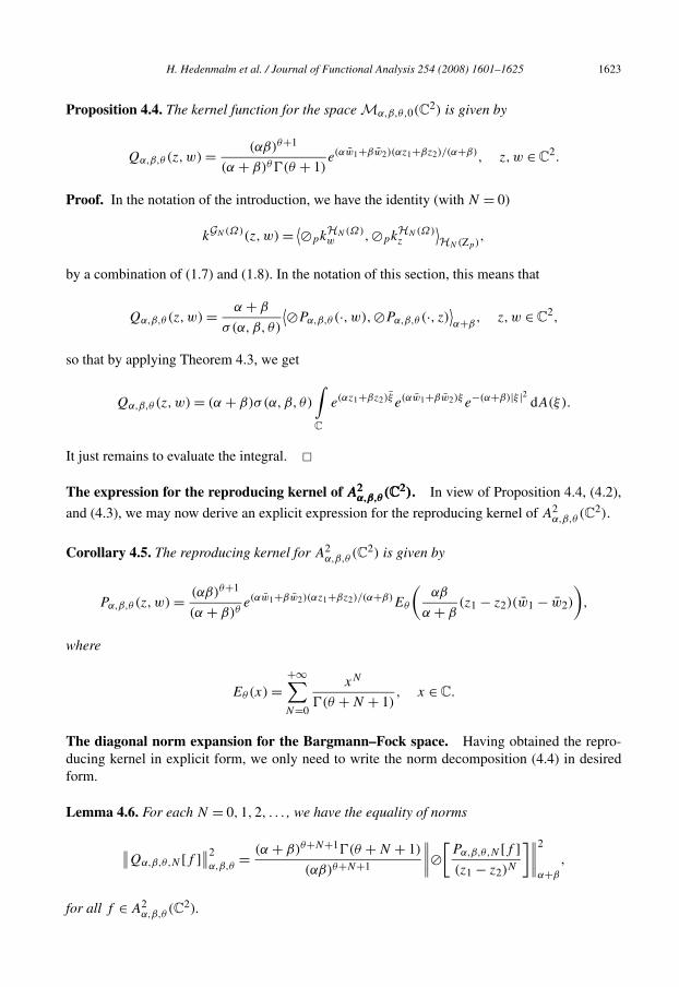
Proposition 4.4. The kernel function for the space Mα,β,θ,0(C2) is given by

Qα,β,θ (z,w) = (αβ)θ+1

(α + β)θ�(θ + 1)e(αw1+βw2)(αz1+βz2)/(α+β), z,w ∈ C

2.

Proof. In the notation of the introduction, we have the identity (with N = 0)

kGN (Ω)(z,w) = ⟨pkHN(Ω)w ,pkHN(Ω)

z

⟩HN (Zp)

,

by a combination of (1.7) and (1.8). In the notation of this section, this means that

Qα,β,θ (z,w) = α + β

σ(α,β, θ)

⟨Pα,β,θ (·,w),Pα,β,θ (·, z)⟩α+β

, z,w ∈ C2,

so that by applying Theorem 4.3, we get

Qα,β,θ (z,w) = (α + β)σ(α,β, θ)

∫C

e(αz1+βz2)ξ e(αw1+βw2)ξ e−(α+β)|ξ |2 dA(ξ).

It just remains to evaluate the integral. �The expression for the reproducing kernel of A2

α,β,θ (C2)A2

α,β,θ (C2)A2

α,β,θ (C2). In view of Proposition 4.4, (4.2),

and (4.3), we may now derive an explicit expression for the reproducing kernel of A2α,β,θ (C

2).

Corollary 4.5. The reproducing kernel for A2α,β,θ (C

2) is given by

Pα,β,θ (z,w) = (αβ)θ+1

(α + β)θe(αw1+βw2)(αz1+βz2)/(α+β)Eθ

(αβ

α + β(z1 − z2)(w1 − w2)

),

where

Eθ(x) =+∞∑N=0

xN

�(θ + N + 1), x ∈ C.

The diagonal norm expansion for the Bargmann–Fock space. Having obtained the repro-ducing kernel in explicit form, we only need to write the norm decomposition (4.4) in desiredform.

Lemma 4.6. For each N = 0,1,2, . . . , we have the equality of norms

∥∥Qα,β,θ,N [f ]∥∥2α,β,θ

= (α + β)θ+N+1�(θ + N + 1)

(αβ)θ+N+1

∥∥∥∥[Pα,β,θ,N [f ](z1 − z2)N

]∥∥∥∥2

α+β

,

for all f ∈ A2α,β,θ (C

2).


Proof. The statement follows from a combination of Lemma 4.1 and (4.6), plus the evaluationof σ(α,β, θ + N). �

All that remains for us to do is to make the right-hand side of the expression in Lemma 4.6sufficiently explicit.

Lemma 4.7. For all k = 0,1,2, . . . , and each f ∈ A2α,β,θ (C

2), we have

∂kz1

[f ] =k∑

n=0

n!(

k

n

)(α

α + β

)k−n

∂k−nz1

[Pα,β,θ,n[f ](z1 − z2)n

]. (4.7)

Proof. We observe that

[∂

jz1Qα,β,θ,N

](z1, (w1,w2)

) =(

α

α + β

)j

∂jz1 [Qα,β,θ,N ](z1, (w1,w2)

).

The rest of the proof is obtained by mimicking the arguments of Lemma 2.6. �It is quite easy to invert Lemma 4.7:

Lemma 4.8. For all N = 0,1,2, . . . and each f ∈ A2α,β,θ (C

2), the equality

[

Pα,β,θ [f ](z1 − z2)N

](z1) =

N∑k=0

(−1)N−k

k!(N − k)!(

α

α + β

)N−k

∂N−kz1

[∂kz1

f](z1), z1 ∈ C, (4.8)

holds for each f ∈ A2α,β,θ (C

2).

Proof. In view of Lemma 4.7, it is enough to check that

N∑k=n

(−1)N−k

k!(N − k)!n!(

k

n

)(α

α + β

)N−n

= δn,N ,

where δn,N is the Kronecker delta. Firstly, we observe that the equality holds for n = N . Sec-ondly, we observe that it is equivalent to show that

N∑k=n

(−1)N−k

k!(N − k)!n!(

k

n

)=

N∑k=n

(−1)N−k

(N − k)!(k − n)! = 0

whenever n < N . The expression in the middle is an (N −n)th difference of a constant function,which of course is 0 for n < N . We are done. �

We now combine our results and obtain the norm expansion for the Bargmann–Fock space.


Theorem 4.9. Let ck,N (α,β) be given by

ck,N (α,β) = (−1)N−k

(N

k

)[α

α + β

]N−k

.

Then, for each f ∈ A2α,β,θ (C

2), we have

‖f ‖2α,β,θ =

+∞∑N=0

(α + β)θ+N+1�(θ + N + 1)

(αβ)θ+N+1[N !]2

∥∥∥∥∥N∑

k=0

ck,N (α,β)∂N−kz1

[∂kz1

f]∥∥∥∥∥

2

α+β

.

Remark 4.10. There is an alternative way to obtain the norm expansion and the explicit ex-pression for the reproducing kernel in the Bargmann–Fock space A2

α,β,θ (C2). The change of

variables {z1 = w1 + βw2,

z2 = w1 − αw2

transforms the norm in A2α,β,θ (C

2) into the expression

‖f ‖α,β,θ = (α + β)2θ+2∫C

∫C

∣∣g(w1,w2)∣∣2|w2|2θ e−(α+β)|w1|2−αβ(α+β)|w2|2 dA(w1)dA(w2),

where g(w1,w2) = f (w1 + βw2,w1 − αw2). The reproducing kernel and the norm expansionabout the hyperplane w2 = 0 with respect to the latter norm can be calculated by separation ofvariables. Shifting back to the original variables (z1, z2), then, we obtain the reproducing kerneland norm expansion for A2

α,β,θ (C2).

References

[1] S. Bergman, The Kernel Function and Conformal Mapping, second, revised ed., Math. Surveys Monogr., vol. V,Amer. Math. Soc., Providence, RI, 1970.

[2] R.G. Douglas, G. Misra, Characterizing quotient Hilbert modules, in: Linear Algebra, Numerical Functional Analysisand Wavelet Analysis, Allied Publ., New Delhi, 2003, pp. 79–87.

[3] H. Hedenmalm, H.B. Korenblum, K. Zhu, Theory of Bergman Spaces, Grad. Texts in Math., vol. 199, Springer-Verlag, New York, 2000.

[4] H. Hedenmalm, S. Shimorin, Weighted Bergman spaces and the integral means spectrum of conformal mappings,Duke Math. J. 127 (2005) 341–393.

[5] S.G. Krantz, Function Theory of Several Complex Variables, Amer. Math. Soc./Chelsea, Providence, RI, 2001.Reprint of the 1992 edition.

[6] W. Rudin, Function Theory in Polydiscs, Benjamin, New York, 1969.[7] W. Rudin, Function Theory in the Unit Ball of C

n, Grundlehren Math. Wiss., vol. 241, Springer-Verlag, New York–Berlin, 1980.

[8] S. Saitoh, Theory of Reproducing Kernels and Its Applications, Pitman Res. Notes in Math., vol. 189, Wiley, NewYork, 1988.

Documents

Norm expansion along a zero variety