Urban-biased trends in Buenos Aires' mean temperature

CLIMATE RESEARCH Clim. Res.

1 Published April 28

Urban-biased trends in Buenos Aires' mean temperature

Vicente Barros, Ines Camilloni

Department of Atmospheric Sciences. University of Buenos Aires. Pabellon II ,2" piso, (1428) Buenos Aires, Argentina

ABSTRACT: The yearly mean temperature in northeastern Argentina is described by a simple model of geographic coordinates and elevation. According to the simulation tests, the mean temperature in a given year at any rural location can be estimated with a RMSE (root-mean-square error) of less than 0.5"C as long as there are data from at least 8 stations in the region. The mean temperature for a 5 yr period can be estimated with an even lower RMSE of less than 0.4 "C. In spite of the severe limitations of the available data, use of the model permits Buenos Aires' urban-rural temperature differences since 1929 to be calculated. During the 1940s and 1950s the urban-rural temperature difference increased linearly, later slowing and reaching a maximum during the 1960s. The decrease in the urban-rural temperature difference after the 1960s could be attributed at least in part to the general warming of the region. An extension of the latter finding to global surface mean temperature suggests the possibility that the presumed global warming is now being masked to a certain extent by the urban heat island effect, contrary to what happened during the first 60 yr of this century.

K E Y WORDS: Urban heat island Global warming . Temperature

INTRODUCTION

The global warming that may currently be under way due to human-induced increase of greenhouse gases has become a public and international issue during recent years, fostering a growing interest in climate change. The lack of sufficient observations during the last century and the beginning of the present one pre- sents a problem for assessing secular climate change. Yet surface temperature is generally used as an indica- tor of global climate change over the past 150 yr, despite the fact that global coverage of meteorological observations during the nineteenth and early twentieth centuries was extremely poor. In addition, many of the available records from that period are from stations which were located either from the outset in urban areas or in places later reached by urban expansion. Thus, these records are affected by the urban heat island, an effect first documented by Howard (1833).

The urban heat island effect has some influence on estimates of global mean temperature trends, which Jones et al. (1989) calculated to be no more than 0.1 "C during the first 8 decades of the twentieth century for

the land masses of the northern hemisphere. This over- estimate is about one-fifth that of the observed warming. On the other hand, while this may be the case for most of the last 150 yr, when the heat island effect was growing due to both urban expansion and energy con- sumption increase, at the present time an opposite bias could be affecting global temperature trend estimates because urban heat island warming could be lower during warmer years. This effect is discussed below in connection with Buenos Aires' heat island trends.

Many causes have been discussed for the urban heat island effect. Howard (1833) believed that urban temperatures were raised by self-heating due to industrial and domestic combustion. Kratzer (1956) attributed the heat island primarily to the blanketing effect of urban atmospheric pollution. Other authors have pointed out the importance of reduced evaporation in cities (Chan- dler 1962, Bornstein 1968). Mitchell (1961) emphasized the role of heat capacity and conductivity of building and paving materials. Cities can absorb larger amounts of heat than rural soils during the day, which then becomes available at night to partially balance the nocturnal radiation loss.

O Inter-Research 1994

34 Clim. Res 4: 33-45, 1994

Oke (1982) lists a number of factors contributing to the urban heat island, including altered energy balance terms leading to positive thermal anomaly: increased absorption of short-wave radiation due to canyon geometry, increased long-wave radiation from the sky due to air pollut~on, decreased long-wave radiation loss because of the reduction of the sky view factor, anthropogenic heat sources, increased sensible heat storage and decreased evapotranspiration due to construction materials, and decreased total turbulent heat transport due to wind speed reduction caused by canyon geometry. As pointed out by Karl & Jones (1989), it is necessary to estimate the urban effect on surface temperature series to achieve a better understanding of global and regional trends. Regional temperature trends are an important tool for relating the observed global increase of temperature to the greenhouse effect as well as for understanding climate variability. However, in many regions of the world there are few if any long temperature series that have not suffered either from changes of location or interrup- tions, or both. In addition, the few long series that are available are mostly from large cities and have been affected by urban growth. This is the case in southern South America, where records from Argentina, Chile and Uruguay have this type of problem. For instance, in a radius of 150 km around Buenos Aires there is only 1 station, Ezeiza, that is located in an approximately rural environment (Fig. 1, Stn 166). Since Ezeiza's records cover only the period since 1947, it remains a problem to assess the evolution of the heat island effect before that date. Even after 1947 there are difficulties because, although Ezeiza is located 30 km from the downtown area, it is now less than 10 km from the

urban borders and could be affected by the urban heat plume. To handle this data situation, we apply a geographic model to construct regional or local series for longer periods than contained in each original record. If the model series simulation is accurate enough, it will permit a calculation and ultimately a filtering out of the urban effect of large cities. The geographical approach was used by Goldreich (1987) to study changes in the spatial distribution of rainfall in Israel, and by Karl et al. (1988) to correct the urban-rural temperature difference (URTD) of pairs of stations sited at different latitudes and elevations. Here, the basic idea is that in a homogeneous region without significant topography or coastal irregularities, yearly surface temperature can be described by a simple function of the geographical coordinates and elevation. For the northeastern part of Argentina a description of this type is explored to model the 'rural' temperature in Buenos Aires, in order to assess the evolution of ~ t s urban heat island effect on the surface mean annual temperature.

MEAN YEARLY TEMPERATURE MODEL

The hypothesis on which the model is based is that yearly mean temperature in a region with smooth horizontal gradients in surface properties can be described by a simple function of latitude, longitude and elevation:

T = T(lat, lon, h) + e (1)

where lat, lon, and h stand for latitude, longitude and height above sea level and e is a departure from the

Present Urban Boundaries

More densely populated

Less densely populated

35" 00'

59" 00' 58" 30' 58" 00' resent meteorological stations

0 20 40 km

I I I Fig. 1 Greater Buenos Aires. Dots rep-

Barros & Camilloni: Urban-biased trends ~n temperature 35

Flg. 2. Base map of Argentina showing the study area , location of meteorological statlons and mean annual surface temperature isotherms ("C), after Hoffman

(1975)

model temperature which is expected to be sufficiently bounded error, if there is a small but still sufficient small to render the model useful. While temperature number of stations in the region. This is crucial for dependence on latitude and elevation could be modeling Buenos Aires' 'rural' temperature since, as expected everywhere, the dependence on longitude shown in Table 1, in many years there are only a few should be considered in those cases where the merid- records available across the entire region. ional extension of coasts or mountain ranges influences the surface temperature.

This hypothesis implies that local peculiarities such GEOGRAPHY AND DATA as type of soil or vegetation, while possibly affecting the annual and daily cycle of temperature, do not intro- The area between 26 and 36" S and 57 and 64" W duce significant changes into the annual mean. This was chosen for applying the model (Fig. 2). It is a part may be the case for regions such as the one studied of northeastern Argentina, a huge plain with only here, as will be seen in the next section. small areas where there are some sparse gentle hills of

We use a geographic model of yearly mean temper- less than 30 m height. The land is used for crops and ature, which is polynomial and includes linear, qua- cattle raising. To the north, there is a transition to open dratic and product terms of the normalized (indicated woodland, also used for cattle raising. The climate is by capitals) variables LAT, LON and H representing moderate to warm and humid with an average temper- latitude, longitude and elevation. The variables are ature of 19°C and an annual range of around 12"C, selected through the stepwise regression procedure of and is considered a Cfa climate in the Koppen classifi- Draper & Smith (1966). Up to 4 variables are included cation. The main geographical features are the huge if each one explains at least an additional 1 % of the Parana and Rio d e la Plata rivers and the delta between total variance. Another hypothesis is that an accept- them. The lack of any significant topography and the able estimate of the regression equation can be smooth vegetation gradients produce small gradients obtained for every year with a small number of sta- in the mean temperature field (Fig. 2). The main variations. In such a case the yearly mean temperature for tion in the mean temperature is with latitude, although any location in the region can be calculated with a some zonal gradient is present due in part to a small

3 6 Cljm. Res. 4: 33-45, 1994 -

2 the mean January and July temperatures (Flg. 3b). - To adjust the yearly mean tempera-

Ue 1.5 ture using geographical parameters, W records from 44 meteorological sta- :: W tions from the 1929 to 1991 period I.

1 were used (Fig. 2, Table 1). In order to

m describe rural temperature conditions, W

2 series from large cities were avoided U m and are not included in Table 1. A few I.

0.5 stations are in cities which now have a E population of more than 25 000, but in S each of these cases the stations are

0 located far from the city, usually at airports. This region is the most devel-

2 oped of Argentina, both economically and culturally. In spite of this, there is not a single complete series for the

p 1.5 63 yr period (Table 1). Only Buenos U

01 Aires (in an urban environment and

0 c thus not included in Table 1) has a Q, L complete record for this penod. This is g 1 illustrative of the difficulties in assess- U W L ing climatic variability in South Amer- 3 ica, where very few long meteorologi- crJ 2 0.5 cal records are available. Since many a records contain only 3 observations W a day at the main synoptic hours,

0 monthly averages were calculated in all series using only 12:00, 18:OO and

0-25 50-75 100-125 150-175 200-225 250-275 24:OO h UTC data, which roughly cor- distances between stations (km) respond to 08, 14 and 20 solar hours.

In northeastern Argentina, these aver-

Fig. 3. Averaged temperature differences between all possible pairs of stations. ages are near the 24 h with a (a) Averaged daily maximum, minimum and mean temperature differences. difference of generally less than 1 'C. (b) Averaged temperature differences for January, July and the annual mean Corrections to the 24 h average

depend on the month and location, and were done according to National Meteorological Service tables.

increase of the surface elevation toward the west and At least 20 d of data were required for the 3 selected to the prevailing northeastern winds that advect warm hours to compute a mean monthly average. In fact, most air from Brazil. of the incomplete months lacked all observations and

Local singularities produced by different surface only a few of them had more than 20 d. Yearly means conditions affect both the mean daily and annual tem- were only computed when all 12 months could be cal- perature cycles, but do not seem to introduce any sig- culated as explained. When these requirements were nificant effect into the mean value. In fact, when the not met, data from that year were considered absent. mean value of the absolute temperature difference Due to the lack of data, a few exceptions were made in calculated between all possible pairs of stations is the 1929 to 1933 period at some stations. In these years, depicted as a function of distance, the results are we estimated up to 2 missing months of the data set of practically zero for distances less than 50 km (Fig. 3). each year, based on the 10 yr average of the same In contrast, differences in the average maximum and months. Since we finally used at least 8 stations in each minimum daily temperatures do not diminish to zero year, these interpolated months amount to no more than for small distances (Fig. 3a), which indicates some sort 2 % of the total data used in the model, and so possible of local influence. The same can be said for the errors associated with them did not introduce any sig- annual cycle, which can be roughly represented by n~ficant difference into the final result.

Barros & Camllloni. Urban-biased trends in temperature 37

'able 1 Surface temperature senes In the study region (1929 to 1991) LAT latitude; LON: longitude, H helght above sea level Asterisks represent usable information

LAT (S) LON ( W )

MODEL VERIFICATION

The 2 points to be verified were that the mean yearly temperature calculated by the model was sufficient to estimate this parameter within certain bounds, and that to do so only required data from a few stations. The last point was necessary so that the model could be used in those years with very few available observations.

The 4 years with the most data were used to verify the model in the region described above. These years

(1968, 1970, 1974 and 1975) included data from at least 24 stations. Table 2 shows the model function calculated for these years, the explained varlance and the RMSE (root-mean-square error). The residual error for each station is more than 0.5 "C in only 2 % of the cases. These few cases do not seem to have any particular geographical distnbution, and they could be due either to observational or data-manipulation errors, or to real singularities in the temperature field.

To check the model's skill in calculating yearly mean temperatures in locations where data could not be fed

C6m. Res. 4: 33-45, 1994

Table 2. Model fit to data, n: number of stations; R2. explained variance

Year n Model ("C) R? RMSE ("C)

1968 24 T = 15.70 + 6.36LAT- 0.94H- 0 . 2 7 ( ~ O N ) ~ 0.97 0.27 1970 24 T = 15.01 + 8.46LAT- 1 ~ ~ ( L A T ) ~ 0.99 0.23 1974 26 T = 14.89 + 5.73LAT- 0 37LON- 1.05H 0.95 0.36 1975 24 T = 16.53 + 2.54LAT- 0.61LON+ 2 . 7 7 ( ~ ~ ~ ) ~ 0.97 0.29

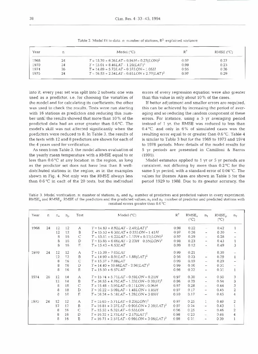
into it, every year set was split into 2 subsets: one was used as a predictor, i.e. for choosing the variables of the model and for calculating its coefficients; the other was used to check the results. Tests were run starting with 16 stations as predictors and reducing this number until the results showed that more than 10 % of the predicted data had an error greater than 0.6"C. The model's skill was not affected significantly when the predictors were reduced to 8. In Table 3, the results of the tests with 12 and 8 predictors are shown for each of the 4 years used for verification.

As seen from Table 3, the model allows evaluation of the yearly mean temperature with a RMSE equal to or less than 0.6OC at any location in the region, as long as the predictor set does not have less than 8 well- distributed stations in the region, as in the examples shown in Fig. 4. Not only was the RMSE always less than 0.6"C in each of the 20 tests, but the individual

errors of every regression equation were also greater than this value in only about 10 % of the cases.

If better adjustment and smaller errors are required, this can be achieved by increasing the period of averaging and so reducing the random component of these errors. For instance, using a 5 yr averaging period instead of 1 yr, the RMSE was reduced to less than 0.4"C, and only in 6 % of simulated cases was the resulting error equal to or greater than 0.6 "C. Table 4 is similar to Table 3 but for the 1969 to 1973 and 1974 to 1978 periods. More details of the model results for 5 yr periods are presented in Camilloni & Barros (1991).

Model estimates applied to 1 yr or 5 yr periods are consistent, not differing by more than 0.2OC for the same 5 yr period, with a standard error of 0.04 "C. The values for Buenos Aires are shown in Table 5 for the period 1929 to 1988. Due to its greater accuracy, the

Table 3 Model verification. n: number of stat~ons; n, and np: number of predictors and predlcted values In every experiment; RMSE, and RMSE,: RMSE of the predictors and the predlcted values; n, and n2: number of predictor and predlcted stations with

residual errors greater than 0.6 "C

Year n n, np Test Model ("C) R2 RMSE, nl RMSEp nl ("Cl ("Cl

1968 24 12 12 A T = 14.83 + 8.92LAT- 2.40(LAT)' 0.98 0.22 - 0.42 1 12 12 B T = 15.53 + 6.30LAT+ 0.22LON- 1.41H 0.97 0.26 - 0.30 -

8 16 C T = 15.51 + 6.22LAT- 1.17H+ 0 . 1 1 ( ~ 0 N ) ' 0.97 0.29 - 0.28 -

8 16 D T = 15.85 + 6.66LAT- 2.23H - 0 . 5 5 ( ~ 0 ~ ) * 0.98 0.23 - 0.43 1 8 16 E T = 15.43 + 6.53LAT 0.99 0.12 - 0.49 3

1970 24 12 12 A T = 15.39 + 7.05LAT 0.99 0.21 - 0.30 -

12 12 B T = 14.90 + 8 . 9 1 L A T 1 , 8 8 ( L ~ T ] ' 0.98 0.23 - 0.29 1 8 16 C T = 15.37 + 7.08LAT 0.99 0.19 - 0.29 -

8 16 L> T = 14.40 + 1 0 . 6 6 L ~ T - 2 . 9 6 ( L ~ T ) ~ 0.99 0.16 - 0.31 -

8 16 E T = 15.50 + 6.57LAT 0.98 0.22 - 0.31 1

1974 26 12 14 A T = 15 74 + 5.71LAT- 0.59LON+ 0.21H 0.97 0.30 - 0.50 3 12 14 B T = 16.55 + 4.75LAT- 1 . 2 3 L O N 0 20(H12 0.96 0.29 - 0.54 3 8 18 C T = 15.48 + 5.95LAT- 0.11LON- 0.96H 0.97 0.28 - 0.44 3 8 18 D T = 16.22 + 5.09LAT- 1.48LON+ 1.85H 0.97 0.17 - 0.45 2 8 18 E T = 16.34 + 5.18LAT- 1.28LON+ 0.89H 0.99 0.17 - 0.45 4

1975 74 12 12 A T = 15 65 + 5 . 7 1 L ~ ~ + 0.23(LON12 0.97 0 25 0.40 2 12 12 B T = 16.81 + 2.37LAT- 0.90LON+ 2.39(LAT12 0.97 0 24 - 0.43 1 8 16 C T = 15.52 + 6.32LAT- 0.53LON 0.96 0.25 - 0.46 2 8 16 D T = 16.32 + 2 . 7 3 L ~ ~ + ~ . ~ ? ( L A T ) ' 0.98 0.23 - 0.46 4 8 16 E T = 16 71 + 2 . 5 7 L ~ ~ - 0.99LON + 3 . 0 6 ( L ~ T ) ~ 0.98 0.21 - 0.39 1

Barros & Carmlloni: Urban-biased trends in temperature

Table 4. Model verification, as in Table 3 but for the 5 yr periods of 1969-1973 and 1974-1978

Year Test Model ('C) R2 RMSE, ("C)

T = 15.84 + 5.94LAT- 0.72(H)' 0 97 0.27 T = 15.99 + 5.55LAT- 0.42(H)2 0.97 0.26 T = 15.67 + 6.10LAT- 1.44H 0.99 0.23 7 - 16.54 + 5.19LAT- 0.93LON 0.98 0.21

T - 15.82 + 5.84LAT- 1.19LON 0.98 0.24 T = 15.58 + 6.34LAT- 0.83LON-t 0 . 4 8 ( L ~ T ) ~ 0.98 0.20 T = 15.88 + 6.06LAT- 1.31 LON- 0.38(H)2 0.97 0.24 T = 15.54 + 5.94LAT- 0.62LON 0.99 0.20

5 yr running mean of the model calculations is more reliable than the yearly model values. This averaging process constrains the use of the model results to only certain problems, but it is still applicable for many pur- poses. For instance, the model can be used to study the evolution of the URTD for large cities of the region, namely Buenos Aires and Rosario, since for these cities the urban heat island effect is greater than the model error (Camilloni & Mazzeo 1987).

Fig. 4. Location of stations used as predictors in some of the verification experiments

1968, y Test D - - _ _ - - - - -

9 8:7

l.08 1J5 ,!

472.

I

..P. . '.--. . .-. . - -

1974, Test E

8 '? 301 '

I 125 ;

451. 127

l 134 I

.-:.--. . ... . -- m

178 ._

MEAN YEARLY REGIONAL TEMPERATURE ESTIMATION

1970, Test E ,.' S -

41 6 --.__.- s;

3.09

-709 m113 ,'

l:' 472.

148 m -t. .. '.___

*. . . -. . -

1975, Test E ;' '--_ -----

% Q ~ 67

82 m m '

67

125 ; 451

, , .d. . '.--. .=.. .-.-.

l 188 .: 178

The yearly mean temperature model, Eq. (l), can be integrated for a particular area and elevation range to calculate its yearly mean regional temperature. Errors in the regional temperature model should be lower than those for individual locations within the region, since the averaging process should eliminate part of the errors due to both real local singularities and random errors.

The true yearly mean regional temperature cannot be determined exactly, but a good estimate may be calculated using a simple arithmetic average in those years when there is good observational coverage of the region. Therefore, in the tests using the 4 years with the most data for model verification, the yearly mean regional temperature was also calculated. The integral bounds were fixed according to the common space covered by the extreme coordinates and elevation of the predictor set of locations (Fig. 5). The integral val-

Table 5. Buenos Aires yearly mean temperature, 1929 to 1988. T,: yearly mean model temperature; To: Central Observatory yearly mean observed temperature; T',: 5 yr mean tempera-

ture produced by the model

Period Tm ( " c ) 7, ("c) Tarn (OC)

40 Clim. Res. 4: 33-45, 1994

years

ues calculated were compared with the arithmetic mean of the whole set of observations in that area (Table 6) . Table 6 shows that with only one exception the errors were less than 0.2'C, even in the cases where the predictor set had only 8 stations. In those cases the RMSE was only 0.03 "C.

Table 6. Mean regional temperature estimate for the region shown in Fig. 5. [ T J : mean regional temperature calculated with all available stations withln the region; Tmodcl: mean regional temperature calculated by model integration; Ta,,,,ye: mean regional temperature calculated with the sta-

tions used in each experiment

Year Test I Tl Tmodel Tsverage

Fig. 5. Yearly mean regional surface temperature calculated with the geographical model for the region depicted on the right

The arithmetic regional average temperatures of the stations within the integral area included in each test are also shown in Table 6. The errors are considerably greater than those of the model, showing that it is better to construct the regional series of yearly mean temperature based on the integration of the model equations.

In the study region, for the 1929 to 1991 period there are at least 8 locations every year with annual mean temperature data. Prior to 1929 there are many years with less than 8 useful records. Therefore, the yearly mean temperature series was constructed starting in 1929 for the common area that included the extreme coordinates of the locations with available data (Fig. 5).

The mean annual temperature for the region depicted in Fig. 5 shows a decrease of 0.5"C until the 1970s, and a similar increase d.uring the last 20 yr. Both the negative trend until the 1970s and the later recov- ery are essentially in phase with other locations in northern Argentina (Hoffmann 1990).

URBAN EFFECT ON BUENOS AIRES MEAN ANNUAL TEMPERATURE

Buenos Aires is one of the world's largest cities. Though its administrative boundaries enclose only 200 km2 and around 3 million people, the urban area in the so-called Great Buenos Aires extends for around 2000 km2 and has 11.3 million inhabitants. Its popu- la.tion grew steadily during the 19th and early 20th centuries, but from 1940 to 1960, the growth was accelerated by industrialization. The surface is relatively featureless, with only minor, gentle differences in height of less than 30 m. It is located at around 35" S

Barros & Camilloni: Urban-biased trends in temperature

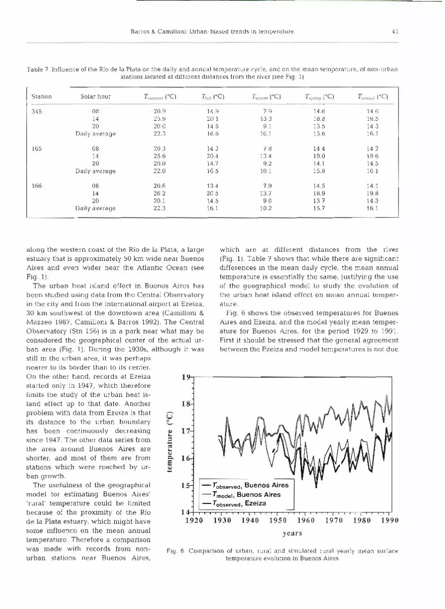
Table 7. Influence of the Rio de la Plata on the daily and annual temperature cycle, and on the mean temperature, of non-urban stations located at different distances from the river (see Fig. 1)

Station Solar hour T,,,,, ( "c ) Tf,u ("C) TWlnte, ("Cl Tsp,,", [ O C ) d o I 348 08 20.9 14.9 7.9 14.6 14.6

14 25.9 20.1 13.3 18.8 19.5 20 20.0 14.8 9.1 13.5 14.3

Daily average 22.3 16.6 10.1 15 6 16.1

08 14 20

Daily average

08 20.6 13.4 7.9 14.5 14.1 14 26.2 20.5 13.7 18.9 19.8 20 20.1 14.5 9.0 13.7 14.3

Daily average 22.3 16.1 10.2 15.7 16.1

along the western coast of the Rio de la Plata, a large estuary that is approximately 50 km wide near Buenos Aires and even wider near the Atlantic Ocean (see Fig. 1).

The urban heat island effect in Buenos Aires has been studied using data from the Central Observatory in the city and from the international airport at Ezeiza, 30 km southwest of the downtown area (Camilloni &

Mazzeo 1987, Camilloni & Barros 1992). The Central Observatory (Stn 156) is in a park near what may be considered the geographical center of the actual urban area (Fig. 1). During the 1930s, although it was still in the urban area, it was perhaps nearer to its border than to its center. On the other hand, records at Ezeiza started only in 1947, which therefore limits the study of the urban heat island effect up to that date. Another problem with data from Ezeiza is that its distance to the urban boundary has been continuously decreasing since 2947. The other data series from the area around Buenos Aires are shorter, and most of them are from stations which were reached by urban growth.

The usefulness of the geographical model for estimating Buenos Aires' 'rural' temperature could be limited because of the proximity of the Rio de la Plata estuary, which might have some influence on the mean annual temperature. Therefore a comparison was made with records from nonurban stations near Buenos Aires.

which are at different distances from the river (Fig. 1 ) . Table 7 shows that while there are significant differences in the mean daily cycle, the mean annual temperature is essentially the same, justifying the use of the geographical model to study the evolution of the urban heat island effect on mean annual temperature.

Fig. 6 shows the observed temperatures for Buenos Aires and Ezeiza, and the model yearly mean temperature for Buenos Aires, for the period 1929 to 1991. First it should be stressed that the general agreement between the Ezeiza and model temperatures is not due

154 1-Tobserved, Buenos Aires I v - Tmodel, Buenos Aires

1 4 1920 1930 1940 1950 1960 1970 1980 1990

years

Fig. 6. Comparison of urban, rural and simulated rural yearly mean surface temperature evolution in Buenos Aires

4 2 Clim. Res. 4 : 33-45, 1994

2 , I Ezeiza since 1947 may mean that the uncertainty is much lower than the error band depicted in Fig. 7. During 1929 to 1942, the difference remained inside the error band and it was lower than 0.5"C In most of those years. A possible reason for this low value is the relatlve position of the Central Observatory with respect to the urban area, as mentioned above. This difference increased during the period 1942 to 1960, showing remarkable agreement with industrial growth and accelerated population expansion. The urban effect on annual temperature after 1960 seems to be between

1920 1930 1940 1950 1960 1970 1980 1990 1.0 and 1 . 5 0 ~ . There is a small nega-

years tive trend in this difference after 1970, probably due to regional warming as

Fig. 7 Evolution of urban-rural yearly mean surface temperature difference discussed in the next section. This in Buenos Aires. Rural temperature was calculated from the geographical effect, together with lower industrial model. The shaded band depicts the RMSE of the 5 yr running mean of this and population growth, may have

difference contributed to stabilize the URTD since 1960. Oke (1973) and other authors used empirical methods to

to any adjustment of the model resulting from the establish relationships between city size and the inclusion of the Ezeiza values as one of its predictors. instantaneous maximum URTD. The parameter chosen In fact, with more than 11 predictor stations during to represent urbanization is the population of the city every year of the 1951 to 1991 period, and in many or metropolitan area. This is not the most desirable years more than 20, the parameters of the model show physical quantity for representing urbanization around only minor changes with the inclusion or the exclusion a meteorological station, but it is one of the few docu- of a single station. rnented statistics that is readily available for the past

While the Buenos Aires observed series shows a century and over much of the world (Oke 1973). clear positive trend of 0.02"C yr-' since 1929 that Several transformations of population were used, e.g. explains as much as the 55% of the total variance, the square-root (Mitchell 1953) and log (Oke 1973, 1976). model displays a slight negative, and non-significant, Karl et al. (1988) produced similar relationships but for trend since that date. Since 1965 there has been a gen- seasonal and annual URTDs in the United States. He era1 warming in the southern part of the region; in the found an approximate square-root (exponent of 0.45) few fairly complete records, namely at the Rosario and dependence of the annual mean differences on popu- Gualeguaychu airports (Stns 133 and 134), there is a lation. Coughlan et al. (1989) presented a similar rela- 0.02 "C yr-' trend. On the other hand, Ezeiza has a pos- tionship for Australian data, but with an even lower itive trend of 0.04 "C yr-' since 1965, while the model exponent (0.3). shows only a 0.02"C yr-' trend since that date. This Fig. 8 depicts the URTD as a function of varylng pop- suggests a growing urban influence on Ezeiza, as ulation size. This difference is lower than those of might be suspected by its proximity to the urban bor- American cities of similar sizes (Karl et al. 1988), even der (Fig. 1). Thus, the model should be preferred to the when the error margin of 0.4 "C is added to the calcu- Ezeiza data for calculating yearly mean URTD, even lated values. There could be 2 main causes for this after 1947. behavior. The first one is the location of the Central

Fig. 7 illustrates the difference between the ob- Observatory with respect to the urban border during served and the model mean yearly temperature of the 1930s and early 1940s, as previously explained. Buenos A~res , the 5 yr running mean of this differ- The second cause could be that the predominant winds ence and the error band of 0.4 "C due to the model's are from the northeast and the city is predominantly limited power in predicting the 5 yr running mean tem- extended in a perpendicular direction along the shore, perature of a location. Notwithstanding the different effectively producing a smaller size for the heat island trends, the general agreement between the model and effect.

Barros & Camilloni: Urban-blased trends in temperature

WARMING TRENDS AND URBAN TEMPERATURES

The URTD of Buenos Aires has decreased since the 1960s, although its population has been continually growing The mixing layer height over Buenos Aires is higher than 700 m most of the time, and even on 90 % of the winter mornings it is higher than 100 m (Scian &

Quinteros 1975). The lack of topographic features that could enhance pollutant concentration and a fair wind regime help the pollutant dispersion. For these rea- sons, air pollution is not a major problem in the city and perhaps does not substantially contribute to the heat island effect. Unfortunately, there are no long pollution records, and only in recent years have there been even sporadic and discontinuous measurements. These are not sufficient to allow any conclusion regarding pollutant concentration change as one of the potential causes for the decreasing trend in the URTD since the 1960s; however, it seems unlikely that pollution has played a significant role in it. To find other possible explanations we must look to changes in meteorological factors.

The dependency of the urban heat island effect on wind, clouds and the near-surface temperature lapse rate has been studied by many authors. Among the first were Sundborg (1950) and Chandler (1965). Lowry (1977) suggested that the weather type situation might be considered in conducting statistical studies of urban heat island effects. Ludwig & Kealoha (1968) found that near-surface temperature lapse rate is highly correlated with the urban mean temperature difference. Lee (1975) calculated the linear regression dependence of London's heat island on rural atmospheric stability, and Godowitch et al. (1985) studied the nocturnal inversion layer in both urban and nonurban environments. It is because of its dependence on low- level stability that the urban heat island effect is greater on the minimum than on the mean temperatures, almost disappearing for the maximum temperatures. Atmospheric vertical stability near the surface is greater during surface cooling processes, such as nocturnal radiational cooling. Mini- mum temperatures usually occur at times when there is pronounced vertical stability in the first few meters above ground. Maximum temperatures are generally observed after several hours of sunshine and are associated with unstable conditions, when the heat is more easily dissipated ver-

tically and later transported aloft by winds. It can be expected that, on average, in middle latitudes during warmer years there will be a greater frequency of unstable conditions. This will be true as long as the warmer years are not strongly associated with more frequent warm advection situations which might be conducive to more stable conditions. With this sole exception, it can be expected that the urban heat island effect in mid-latitudes will be lower during warmer years. Therefore, a negative correlation between annual mean URTD and annual mean rural temperature could be anticipated, as long as the rural temperatures represent regional atmospheric conditions.

In case of global warming, a decrease of the meridional surface temperature gradients is expected, as the result of the predicted greater warming at high latitudes for both hemispheres. This is a point on which the more advanced general circulation models agree without exception (Houghton et al. 1990). Thus, the lower meridional temperature gradient and temperature advection with increasing global temperature will favor more unstable conditions and a reduction of the urban heat island effect.

The Buenos Aires yearly mean temperature produced by the geographic model was used to test the anticipated negative correlation between URTD and rural temperature. To filter out the growth of the urban effect, it was removed from the URTD after modeling URTD with a linear function and with a more realistic

6 population, X 10

Fig. 8. Buenos Aires urban-rural temperature difference calculated from the geographical model as a function of population. Error bars represent the same

RMSE as in Fig. 7

44 Clim. Res. 4: 33-45, 1994

Table 8. Correlations and linear regression coefficients between urban-rural temperature difference (URTD) and rural temperature as calculated with the model (1929 to 1991) and observed in Ezeiza (1951 to 1991). Reduction of URTD explained by the

regression equatlon is also shown

R Significance Regression Reduction of level (%) coefficient URTD ("C) 1

URTD VS Tmodcl -0.50 URTDlLnear "end ltlrered VS Tindel -0.65 URTDquadrallc bend fzllered Tmodel -0.51 URTD VS TE,,, -0.57 URTDbnear trend llltered VS T~zekza -0.68 URTDq~adra$~c tmnd lrllered VS T E h ~ r a -0.35

adjusted quadratic function that reaches its maximum at the end of the 1960s. A similar calculation was done using Ezeiza as a rural station during the 1951 to 1991 period. Both results are shown in Table 8. A remarkable significant negative correlation exists, even after removal of the trend. The correlation increases substantially when the Linear URTD trend is removed. The removal of the linear trend may enhance the negative correlation because, for the 1980s -one of the warmer periods - the decline in URTD is artificially amplified by this process. In any event, the negative correlation is still high when the trend is removed using a quadratic adjustment.

Table 8 also shows the linear regression coefficients of the URTDs as a function of the model and Ezeiza temperatures. When the quadratic trend of the predicted variable is removed, the resulting regression equations can be used to estimate the response of URTD to a change in 'rural' temperature. The Ezeiza and model warming from 1965 to 1991 was calculated from a linear fit to be 1.1 and 0.6"C respectively. According to these results, the decrease in URTD due to regional warming since 1965 could be estimated to be at least 0.2"C. This is enough to explain the observed URTD decrease. Therefore it can be con- cluded that the positive trend in regional temperature over the last 30 yr is at least one possible cause for the decrease in URTD in Buenos Aires.

lf the negative correlation observed between the urban-rural yearly mean temperature difference and the rural yearly mean temperature exists in other regions of the world, this behavior might be helping to compensate for the artificial warmlng due to the still- growing urbanization in most of the Third World, espe- cially in Latin America and Africa. Failure to recognize this possible behavior could contribute to masking the possible global warming presently under way, since the urban effect in temperature is not only observed in large cities. The mean URTD was found to depend on population for the United States as a near-square-root function (Karl et al. 1988). Though the specific function

may change for other regions, there is little doubt about the dependence on city population, even for small cities. Therefore, even if large cities are avoided when calculating the mean global temperature, the urban effect would still be present because many of the remaining observations would be from stations sited in urban or quasi-urban environments.

While this situation may have produced an over- estimate of less than O.l°C in the global temperature trend until the 1960s or 1970s (Jones et al. 1989). the combined effect of lower urban growth in the mid- latitudes, together with global warming of the atmosphere, may be contributing to an underestimation of the present warming.

CONCLUSIONS

The geographical model of mean surface temperature, based on regression analysis techniques, has proven to be a useful tool for the simulation of local and regional temperature series in northeastern Argentina, a flat area with small gradients in surface properties at a regional scale. The model's data requirements are low, allowing for its use in those years when there are as few as 8 series in the region.

The model's rural temperature estimate for Buenos Aires allows Ezeiza to be replaced as the rural refer- ence for Buenos Aires (which is desirable due to Ezeiza's proximity to the urban border), and it permits the yearly mean URTD to be extended backward from 1947 to 1929.

Since 1960, the mean URTD of Buenos Aires has not increased and in fact has shown a slow decrease. Popu- lation has almost doubled in the last 30 yr, so the expla- nation for URTD behavior may be found in a change of meteorolog~cal conditions. The correlation between yearly mean rural temperature and URTD is significantly negative, indicating that warmer years are associated wi.th lower URTDs. Therefore, the regional warming observed since 1960 could explain, at least partially, the decrease in the URTD of Buenos Aires.

Barros & Camilloni Urban-biased trends in temperature 4 5

LITERATURE CITED

Bornstein, R D (1968). Observations of the urban heat island effect in New York City. J , appl. Meteorol 7 . s75 582

Camilloni, I . , Barros, V. (1991). Analysis of thermal effects of urbanization. In: Alvarez, S . , et al. (eds.) Architecture and urban space. Kluwer Academic Publishers, Dordrecht, p 47-52

Camilloni, I . , Barros, V (1992) Anal~sis del comportanliento d e la temperatura en series urbanas en la Republics Argentina Prepnnts of the Fifth lnteramerican Meteoro- logical Congress, Madrid, 1992. Asociacion Meterologica Espanola, Madrid, p. 196-200

Camilloni, I., Mazzeo, N (1987). Algunas caracteristicas ter- micas d e la atmosfera urbana d e Buenos Aires. Prepnnts of the Second Interamerican Meteorological Congress, Buenos Aires, 1987. Centro Argentino d e Meteorologos, Buenos Aires, p 14.2.1-14.2.5

Chandler, T. J . (1962) London's urban climate Geogr. J . 127: 279-302

Chandler, T. J (1965) The cllrnate of London. Hutchinson & Co., London

Coughlan, M. G . , Tapp, N. R., Kninmonth, W. R. (1989). Trends in Australian temperature records. In: Observed climate variations and change. contributions ln support of Section 7 of the 1990 IPCC Scient~fic Assessment Inter- governmental Panel on Climate Change, p. 1-28

Draper, N., Smith, H. (1966). Applied regression analysis John Wlley & Sons, New York

Godowitch, J. M., Ching, J . K S., Clarke, J . F. (1985). Evolu- tion of the nocturnal inversion layer at an urban and nonurban location. J Clim appl. Meteorol 24. 791-804

Goldreich, Y (1987). Advertent/inadvertent changes in the spatial dlstnbution of rainfall in the central coastal plain of Israel Clim Change 11 361-373

Hoffmann, J A J (1975) Chmatlc atlas of South Amenca World Meteorological Organization, Geneva

Hoffmann J A J (1990) De las vanaciones d e temperatura e n Argentina y la zona subantart~cci adyacente desde 1903 a 1985 In Preprints of the F ~ r s t Latin Amencan Confer-

Ed~tor. V Meentemeyer, Athens, Georg~a, USA

ence on Geophysics and Spatial Antarctic Research, Buenos Aires, 1990 Centro Latinamericano d e Fisica, Buenos Aires, p 160-168

Houghton, J. T , Jenklns, E J , Ephraumus, J . J . (eds ) (1990). Climatic change: the I P r r Scientific Assessment Cam- brtdge University Press, Cdrribndge

Howard, L (1833) Climate of London deduced from meteorological observations, 3rd edn. Harvey and Darton, London

Jones, P D., Kelly, P. M., Goodess, C. M., Karl, T (1989) The effect of ur-ban warming on the Northern Hemisphere temperature average J . Clim. 2 285-290

Karl, T R. , Diaz, H. F., Kukla, G. (1988) Urbanization: lts detection and effect in the United States climate record. J . Clim. 1 . 1099-1123

Karl, T R., Jones, P D (1989). Urban blas in area averaged surface air temperature trends. BuU. Am. Meteorol Soc 70. 265-270

Kratzer, A. (1956). Das Stadtkllma, 2nd edn Friedr. Vleweg & Sohn, Braunschweig

Lee, D. 0. (1975). Rural atmosphenc stability and the intensity of London's heat island. Weather 30: 102-109

Lowry, W. P. (1977). Empirical estlmatlon of urban effects on problem analysis. J. appl Meteorol 16: 124-135

Ludwig, F. L , Kealoha, J . H S. (1968). Urban climatological studies. OCD-DAHC-0936. Stanford Research Institute, Menlo Park, CA

Mitchell, J. M. (1953). On the causes of instrumentally observed secular temperature trends J. Meteorol. 10.244-261

Mitchell, J. M. (1961). The temperature of cities. Weatherwise 14 224-229

Oke, T. R . (1973). City size and the urban heat ~ s l a n d . Atmos. Environ. 7- 769-779

Oke, T. R. (1976). The distinction between canopy and boundary layer urban heat islands. Atmosphere 14: 268-277

Oke, T. R. (1982) The energetic basis of the urban heat island. Q. J . R. Meteor Soc. 108 1-24

Scian, B. V., Quinteros, S. R (1975). Capa d e mezcla e n la ciu- dad d e Buenos Aires. Meleorologica 6/7 145-156

Sundborg, A. (1950) Local climatological studies of the temperature conditions in an urban area Tellus 2: 222 -232

Manuscript first received: Apl-il 22, 1993 Revised verslon accepted: December 17, 1993

Documents

Urban-biased trends in Buenos Aires' mean temperature