Unpacking contemporary English blends: Morphological

Unpacking contemporary English blends: Morphological structure, meaning, processing

by

Natalia Beliaeva

A thesis

submitted to the Victoria University of Wellington

in fulfilment of the requirements for the degree of

Doctor of Philosophy

Victoria University of Wellington

(2014)

iii

Abstract

It is not coincidental that blend words (e. g. nutriceutical ← nutricious + pharmaceutical,

blizzaster ← blizzard + disaster) are more and more often used in media sources. In a

blend, two (or sometimes more) words become one compact and attention-catching

form, which is at the same time relatively transparent, so that the reader or listener can

still recognise several constituents in it. These features make blends one of the most

intriguing types of word formation. At the same time, blends are extremely challenging

to study. A classical morpheme-based morphological description is not suitable for

blends because their formation does not involve morphemes as such. This implies two

possible approaches: either to deny blends a place in regular morphology (as suggested

in Dressler (2000), for example), or to find grounds for including them into general

morphological descriptions and theories (as was done, using different frameworks, in

López Rúa (2004b), Gries (2012), Arndt-Lappe and Plag (2013) and other studies). The

growing number of blends observed in various media sources indicates that this

phenomenon is an important characteristic of the living contemporary language, and

therefore, blends cannot be ignored in a morphological description of the English

language (and many other typologically different languages). Moreover, I believe that

the general morphological theory has to embrace blends because of the vast amount of

regularity observed in their formation, despite their incredible diversity.

The formation of blends involves both addition and subtraction, which relates

them both to compounds and to clippings. This research aims to clarify the

morphological status of blends in relation to the neighbouring word formation

categories, in particular, to the so-called clipping compounds (e.g. digicam ← digital +

camera). To approach this problem, I compiled a collection of English neologisms

formed by merging two (in some cases, more) words into one, and analysed their formal

and semantic properties. The results of this analysis were used to distinguish between

blends and clipping compounds, and also to justify the classification of blends according

to different degrees of formal transparency (using the principles of Lehrer’s (1996,

2007) classification). The strength of the association between blends (or clipping

compounds) and their source words was then assessed in two experiments: an online

survey involving evaluating definitions of blends and clipping compounds, and a

psycholinguistic experiment involving a production and a lexical decision task. The

iv

experimental findings show that recognisability of the source words of blends and

clipping compounds has significant influence both on the evaluation of their definitions

and on their processing. The main implication of the experimental results is that blends,

unlike clipping compounds, are closer to compounds than to clippings. In addition to

this, significant differences are revealed between blends containing full source words

and blends containing only parts of them. Therefore, the structural type of blend, as

defined in this study, is a factor which has strong influence on the processing of blends

and their source words.

v

Acknowledgements

This thesis primarily concerns my contribution to the knowledge about blends. This

contribution, however, seems tiny in comparison to the amount of knowledge and

experience I acquired during my PhD journey. These were given to me by the people

who surrounded me at various stages of this project to a much greater extent than taken

from books and journals. To all these people, I express my heartfelt gratitude.

First of all, I am grateful to my primary supervisor, Professor Laurie Bauer, who did

much more for this research project than fulfil his supervisory duties. His friendly

support, inspiring feedback, and his genuine interest not only in the formation of blends,

but also in my own formation as an independent researcher have been crucial for the

progress of this thesis. I am also indebted to my secondary supervisor, Associate

Professor Paul Warren, who provided extremely valuable feedback at all the stages of

the experimental part of this project, and whose comments on my writing inspired me to

address the trickiest aspects of statistical analysis instead of avoiding them. I am further

grateful to Dr. Anna Siyanova, who agreed to join the supervisory team when this project

was well under way. Her expertise in experimental studies was very valuable for

shaping my own experimental methodology. I am also very grateful to her for positive

attitude to all aspects of my work, which was vital for getting me through bumps on this

road. I would like to add a special thank you to Professor Ingo Plag, who provided

stimulating feedback and advice at a crucial stage of my PhD, and who introduced me to

the exciting world of statistical analysis in R.

I also wish to thank my examiners Prof. Jen Hay, Dr Paula López Rúa and Dr. Carolyn

Wilshire for their genuine interest in my work and their insightful comments.

I would like to thank all the staff of School of Linguistics and Applied Language Studies

for being a lively, inspiring and supportive academic community. I also thank the School

for providing opportunities to gain teaching experience, and I must confess that I

learned at least as much from the courses I worked on as the students did. I am grateful

to all the teaching and the administrative staff of SLALS for making life at the School

easier in all sorts of ways, from sorting out administrative issues smoothly and almost

unnoticeably, to relaxing conversations over innumerable cups of coffee we had

together. And, of course, I am sincerely grateful to my fellow PhD students Anna Piasecki,

Sharon Marsden, Ewa Kusmierczyk, Kieran File, Keely Kidner, TJ Boutorwick, Deborah Chua

and many others, who provided valuable feedback during the exciting sessions of the thesis

vi

group, and who helped make Wellington my second home. A special thanks to Liza Tarasova,

for making my landing in New Zealand as soft as it could possibly be.

This research project would not have been possible without the financial support of the

grant from the Royal Society of New Zealand through its Marsden Fund to Laurie Bauer,

and also without the research grants of the Faculty of Humanities and Social Sciences.

Undertaking this research project would be much less exciting and much more solitary

without the support of my family and friends both in New Zealand and in Russia. I would

like to thank Dr Elena Myagkova, who first inspired my interest in linguistic research,

and Dr Vera Pishchalnikova, my mentor and supervisor of the Candidate of Philological

Sciences thesis. Words can hardly express my gratitude to my parents for their love and

support, and to my husband Aleksandr and my daughter Polina for constantly reminding

me there is life outside the PhD.

You gave me much more than I could ever give back. Thank you.

vii

Papers and presentations derived from this research

Journal papers:

Beliaeva, N. (2014). A study of English blends: From structure to meaning and back

again. Word Structure, 7(1), 29–54.

Conference presentations:

Beliaeva, N. (2012). The chemistry of blends: How people merge words together.

Presented at the 2nd Auckland Postgraduate Conference on Linguistics and Applied

Linguistics, Auckland, June 30.

Beliaeva, N. (2012). The power of slanguage: Form and meaning of English blends.

Presented at the Data-Rich Approaches to English Morphology, Wellington, July 4–6.

Beliaeva, N. (2012). The power of slanguage: Conceptual integration on the word

formation level. Presented at the 4th UK Cognitive Linguistics Conference, London, July

10–12.

Beliaeva, N. (2013). From phonology to morphology, from morphology to semantics: A

study of English blends. Presented at Morphology and its Interfaces, Lille, September

12–13.

viii

ix

Contents Abstract.............................................................................................................................................................. iii

Acknowledgements ......................................................................................................................................... v

Papers and presentations derived from this research ................................................................... vii

List of tables ................................................................................................................................................... xiii

List of figures .................................................................................................................................................. xv

Chapter 1. Introduction ................................................................................................................................ 1

1.1. Background and motivation of the thesis ............................................................................ 1

1.2. Aims of the thesis .......................................................................................................................... 2

1.3. The structure of the thesis ......................................................................................................... 3

Chapter 2. The dramality of the blendaverse: Research on blends .............................................. 5

2.1. Early classifications and classical discrepancies ................................................................... 5

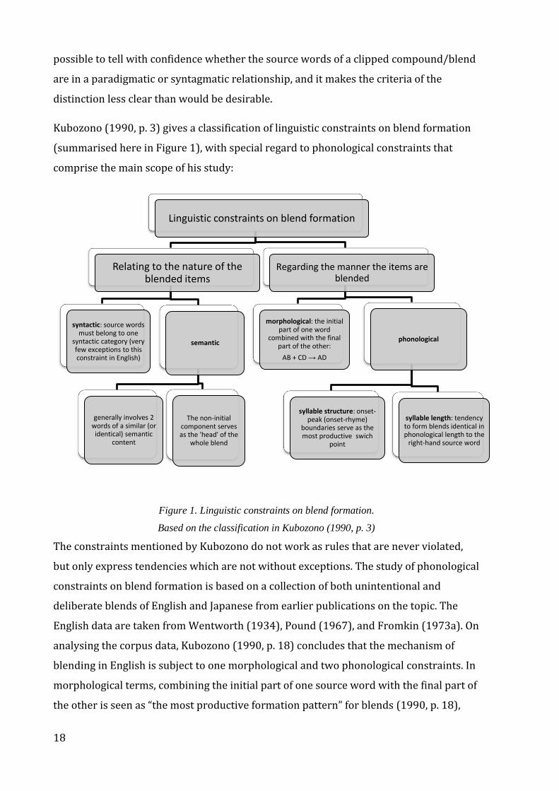
2.2. A closer look at the mechanism of blending .......................................................................... 17

2.3. Grammatical or extragrammatical? .......................................................................................... 29

2.4. The position of blends among the neighbouring morphological categories ............ 31

2.5. Gaps and beacons ............................................................................................................................ 41

Chapter 3. Basic terminology and rationale ....................................................................................... 45

3.1. Approach to defining blends ....................................................................................................... 45

3.2. The terminological toolkit and the scope of the study ...................................................... 47

Chapter 4. Lexical data: From structure to meaning and back again ....................................... 51

4.1. Data sampling and methodology ............................................................................................... 51

4.2. Phonological properties ................................................................................................................ 59

4.2.1. Data and methods ................................................................................................................... 59

4.2.2. Results and discussion .......................................................................................................... 62

4.3 Structural properties: Interaction with phonology ............................................................. 68

4.3.1. Data and methods ................................................................................................................... 68


4.4. Semantic properties: Interaction with structure ................................................................ 75

x

4.4.1. Data and methods ................................................................................................................... 75


4.5. Interim conclusions: Phonological and semantic factors which influence the

structure of blends .................................................................................................................................. 80

Chapter 5. Deconstructing blends: Insights from psycholinguistic and cognitive studies

............................................................................................................................................................................. 85

5.1. Cognitive mechanisms of blending revealed in the form of blends ............................. 85

5.2. What factors determine recognisability?............................................................................... 91

5.3. Methodological prerequisites for an experimental study of blends ......................... 102

Chapter 6. What can be predicted from the way predictionary and other blends are

defined? A web-based study. ................................................................................................................. 105

6.1. Objectives and hypotheses of the study ............................................................................... 105

6.2. Data and methods ......................................................................................................................... 108

6.2.1. Participants ............................................................................................................................. 108

6.2.2. Stimuli ....................................................................................................................................... 108

6.2.3. Procedure ................................................................................................................................ 109

6.2.4. Methods of analysis ............................................................................................................. 112

6.3 Results and discussion ................................................................................................................. 113

6.4. Interim conclusions: Perception and understanding of blends and clipping

compounds............................................................................................................................................... 130

Chapter 7. Can you find an academic in an acatramp? Priming effect of blends and

clipping compounds on the processing of their source words................................................. 135

7.1. Background and rationale ......................................................................................................... 135

7.2. Participants ..................................................................................................................................... 137

7.3. Stimuli................................................................................................................................................ 138

7.4. Procedure ......................................................................................................................................... 139

7.4.1. Task 1: An identification and production task .......................................................... 139

7.4.2. Task 2: A lexical decision task ......................................................................................... 141

7.5. Methods of data analysis ............................................................................................................ 143

xi

7.5.1. Task 1 ........................................................................................................................................ 143

7.5.2. Task 2 ........................................................................................................................................ 144

7.6. Results ............................................................................................................................................... 146

7.6.1. Identification and production task results ................................................................. 146

7.6.2. Lexical decision task results ............................................................................................. 158

7.7. Interim conclusions: Recognisability and recognition ................................................... 170

Chapter 8. Synthesis and conclusions ................................................................................................ 175

8.1. The design of this research revisited .................................................................................... 175

8.2. The main findings of the thesis ............................................................................................... 176

8.3. The implications of the research ............................................................................................ 184

8.3.1. Finding room for blends in English morphology: Implications for taxonomic

studies ................................................................................................................................................... 184

8.3.2. Finding room for blends in your ‘mind palace’: Implications for the studies of

word processing ............................................................................................................................... 186

8.4. The limitations of the study and the recommendations for future research ........ 188

References .................................................................................................................................................... 191

Appendix 1. Lexical data ......................................................................................................................... 201

Appendix 2. Ethics Approval ................................................................................................................. 213

Appendix 3. Information sheet for participants of the web-based survey .......................... 215

Appendix 4. Survey stimuli .................................................................................................................... 217

Appendix 5. Item variables used in the survey .............................................................................. 233

Appendix 6. Regression models predicting the responses in the survey ............................ 235

Appendix 7. Information sheet for the participants of the experiment ............................... 249

Appendix 8. Consent form for the participants of the experiment ......................................... 251

Appendix 9. Experimental stimuli ....................................................................................................... 253

Appendix 10. Item variables used for the analysis of experimental data ............................ 255

Appendix 11. Regression models predicting the response to the experimental stimuli 257

xii

xiii

List of tables

Table 1. Derivatives and compounds formed by adding recently established morphs .... 52

Table 2. Structural classification of lexemes in the collected corpus ....................................... 56

Table 3. Structural classification of lexemes in the collected corpus, revised ..................... 58

Table 4. Structural types of blends with non-central overlap ..................................................... 59

Table 5. The syllable structure of the four main types of blends ............................................... 70

Table 6.The distribution of the data with regard to the semantic origin and the type of

source word combinations attested in COCA..................................................................................... 77

Table 7. Source words combinations extracted from COCA ........................................................ 77

Table 8. Survey stimuli ............................................................................................................................ 109

Table 9. Observed median responses to definitions of different types of target words 116

Table 10. Likelihood ratio tests comparing models predicting the response in the main

survey with increasingly complex random effects structure ................................................... 124

Table 11. The effects of item and participant factors on the response in the main survey

........................................................................................................................................................................... 124

Table 12. Likelihood ratio test comparing the model with simple effects of blend type

and definition type with the model including the interaction of the two factors ............. 126

Table 13. The effects of blend type and definition type on the response in the main

survey ............................................................................................................................................................. 127

Table 14. Likelihood ratio test comparing the model with simple effects of blend type

and definition type with the model including the interaction of the two factors

(combined data from the main and the additional survey) ...................................................... 129

Table 15. Simple effects of blend type and definition type in the main and the additional

survey ............................................................................................................................................................. 129

Table 16. The effects of blend type and definition type, and the interaction of the two

factors in the main and the additional survey ................................................................................ 129

Table 17. Arrangement of word stimuli into groups according to priming conditions. 142

Table 18. Percentage of correct answers in Task 1 ...................................................................... 147

Table 19. The output of the regression model predicting SW1 naming ............................... 148

Table 20. The output of the regression model predicting SW2 naming ............................... 148

Table 21. The output of the regression model predicting SW2 naming in Group 1 ........ 149

Table 22. Likelihood ratio tests comparing models with splinter frequency and relative

frequency predicting SW1 naming ...................................................................................................... 151

xiv

Table 23. Likelihood ratio tests comparing models with splinter frequency and relative

frequency predicting SW2 naming ...................................................................................................... 151

Table 24. Likelihood ratio tests comparing models with correlating predictors of SW1

naming ............................................................................................................................................................ 152

Table 25. The output of the final model predicting SW1 identification ................................ 153

Table 26. Likelihood ratio tests comparing models with correlating predictors of SW2

naming ............................................................................................................................................................ 155

Table 27. The output of the final model predicting SW2 identification ................................ 156

Table 28. The output of the model predicting RT in Task 1 ...................................................... 157

Table 29. Mean reaction time to target words in Task 2 for different priming conditions,

millisecs (SD) ............................................................................................................................................... 160

Table 30. The output of the model predicting RT to words in Task 2, with simple effects

only .................................................................................................................................................................. 161

Table 31. The output of the model predicting RT to words in Task 2, for

PrimeShownTRUE condition ................................................................................................................. 162

Table 32. Likelihood ratio tests comparing models with increasingly complex structure

........................................................................................................................................................................... 163

Table 33. The output of the final model predicting RT to words in Task 2 ......................... 163

Table 34. Mean reaction time to nonwords in Task 2, millisecs (SD) .................................... 165


........................................................................................................................................................................... 166

Table 36. The output of the final model predicting RT to nonwords in Task 2 ................. 166

Table 37. The proportion of errors in Task 2 for different priming conditions,%. .......... 169

Table 38. The output of the model predicting error rate for words in Task 2 ................... 169

Table 39. The output of the model predicting error rate for nonwords in Task 2 ........... 170

xv

List of figures

Figure 1. Linguistic constraints on blend formation. ...................................................................... 18

Figure 2. The proportion of the first (SW1) and the second (SW2) source words

preserved in formations of different structural types.................................................................... 60

Figure 3. Boundary phonemes in blends and clipping compounds. ......................................... 61

Figure 4. Correlation between the length of the splinters and the length of the source

words. ................................................................................................................................................................ 63

Figure 5. Correlation between the length of the left splinter of the first source word (W1)

and the frequency rank of the boundary phonemes. ...................................................................... 65

Figure 6. Correlation between the length of the right splinter of the second source word

(W2) and the frequency rank of the boundary phonemes. .......................................................... 66

Figure 7. Correlation between the length of the left splinter of the second source word

(W2) and the frequency rank of the boundary phonemes in AC formations. ....................... 66

Figure 8. The results of the decision tree analysis of the influence of the switch point

placement and the phonological overlap on the structural type of a blend in the YN

group .................................................................................................................................................................. 72

Figure 9. The prosodic pattern of source words repeated in a blend as the predictor of

the structural type of the blend ............................................................................................................... 74

Figure 10. Frequency and type of source word combinations as the predictor of the

semantic type of blends. ............................................................................................................................. 78

Figure 11. Frequency and type of source word combinations as the predictors of the

structural type of blends. ........................................................................................................................... 79

Figure 12. The distribution of responses by the age group of the participants (a) and by

their education level (b).. ........................................................................................................................ 114

Figure 13. The distribution of responses by structural type of the target word (a) and by

definition type (b). ..................................................................................................................................... 115

Figure 14. A decision tree analysis of the response with item factors as independent

variables. ....................................................................................................................................................... 119

Figure 15. A decision tree analysis of the response to the main survey, with item and

participant factors as independent variables. ................................................................................ 121

Figure 16. A decision tree analysis of the response to the main survey, with item factors

as independent variables. ....................................................................................................................... 122

Figure 17. A quantile-to-quantile plot of the residuals of the regression model predicting

the responses in the main survey. ....................................................................................................... 125

xvi

Figure 18. Regression coefficients for response by blend type and definition type, in the

model with interaction of these experimental variables. ........................................................... 128

Figure 19. Regression coefficients for response by blend type and definition type, in the

model with interaction of these experimental variables. ........................................................... 130

Figure 20. The experimental procedure: Task 1 ............................................................................ 140

Figure 21. The experimental procedure: Task 2. ........................................................................... 141

Figure 22. Correlation matrix of a selection of item variables. ................................................ 150

Figure 23.The interaction of prime type and the relative frequency of SW1 splinter in the

model predicting SW1 naming in Task 1. ......................................................................................... 154

Figure 24. The distribution of RT in Task 2. .................................................................................... 159

Figure 25. Correlation matrix of a selection of target variables. ............................................. 162

Figure 26. The interaction of prime type and priming condition in the model predicting

RT in Task 2. ................................................................................................................................................. 164

Figure 27. The interaction of prime type and priming condition in the model predicting

RT to word targets (left panel) and nonword targets (right panel) in Task 2. .................. 168

1

Chapter 1. Introduction

1.1. Background and motivation of the thesis

A blend word used in advertisement (e.g. nutriceutical) or in a title (e.g. Lehrer’s (2007)

Blendalicious) is both attention-catching and thought-provoking. Putting together two

words to form a compound such as sugar bowl is one of the most straightforward ways

to form a new lexeme. A more complex and less frequent way of making one word from

two (or sometimes more, e.g. Christmahanukwanzadan) is merging them together so

that part of the material is lost in the process. Blends are formed in such a way that a

well-formed blend has the phonotactic structure of a simplex word, as observed, for

example, in Tomaszewitz (2012). At the same time, the constituent words remain

recoverable from the form of the blend (Gries, 2004a). These, among other, properties of

blends make them one of the most intriguing types of word formation. It has to be noted

that there is no agreement in the linguistic literature as to whether or not blending is a

productive process of regular word formation. One of the arguments to the contrary is

that the exceptional formal diversity of blends makes it appear that their formation is

completely unpredictable.

The considerations above explain why blends are extremely challenging to study. A

classical morpheme-based morphological description is not suitable for blends because

their formation does not involve morphemes as such. This situation implies two possible

approaches: either to deny blends a place in regular morphology, or to adjust

morphological description in order to embrace this phenomenon. The literature has

examples of both approaches. On the one hand, blends have been analysed as irregular,

creative formations (assuming that creativity is opposed to morphological productivity,

following Bauer’s (2001, p. 64) terminology), and hence excluded from morphological

analysis (Dressler, 2000; Mattiello, 2013). On the other hand, the surface structure of

blends, their phonology and semantics have been analysed in order to find grounds for

including them in general morphological descriptions. For example, the mechanisms of

blending have been investigated within constraint-based theoretical frameworks such as

Optimality Theory (Arndt-Lappe and Plag, 2013) and Schema Theory (Kemmer, 2003).

With regard to the relationship between blends and other word formation types, one

way of classifying them is as an intermediate link between compounding and clipping

(López Rúa, 2004b), or, in a wider sense, between productivity and creativity. Grey areas

2

like these, although difficult to research and yielding controversial results, can provide

insights into the different areas they adjoin. Hence, studying blends is not only

intellectually provocative, but potentially theoretically and practically valuable.

1.2. Aims of the thesis

With the assumption that blends lie in a border region between several morphological

categories, the primary aim of this research is to locate where exactly. In particular, the

purpose of this study is to investigate whether blending as a word formation process is a

type of compounding, a type of clipping, a combination of both processes, or neither of

them. This, in turn, leads to a question of whether and to what extent blends are

different from so-called clipping compounds which, like blends, have features in

common with both compounding and clipping.

Analysing the literature on the topic reveals not only the different and often

controversial views on blends mentioned above, it also makes clear that the definition of

blends and the criteria for including lexemes in this category have changed considerably

over time. Moreover, contemporary studies of blends are often based on lexical data

from earlier publications, which can be problematic for two reasons. First, a lot of

lexemes cited as blends in early studies may no longer be analysable as such because the

semantic link between the blend and the blended words may no longer be salient.

Second, the analysis of the blends, that is, the words they originate from, and the way

they are blended, may be biased by the views of the researchers who collected the

original data. The first aim of this research, therefore, is to describe blends as a

morphological phenomenon as accurately and objectively as possible, and to make this

description reflect the contemporary state of blends in the English language. Of course, it

is not possible to avoid relying on earlier theoretical accounts and practical methods. At

various stages of this study, I have made decisions driven by earlier findings, and

adopted definitions and theoretical assumptions provided by earlier research. However,

an important decision concerning my approach to data collection and analysis was to

compile a collection of contemporary blends from original sources other than linguistic

publications, and to analyse them as impartially as possible. Restricting the analysis to

comparatively recent formations comes at the cost of losing a considerable amount of

lexical data (many earlier studies analysed bigger collections of blends because they

included well-established blends alongside new ones). However, the observations and

3

generalisations made on the basis of neologisms can help to provide a more accurate

account of the formation and functioning of blends in contemporary language.

It has often been pointed out in literature (e.g. Gries, 2006; Bauer, 2012) that providing a

structural, phonological and/or semantic taxonomy of blends may not be a sufficient

way of analysing them, particularly because they are so diverse. To understand the

nature of this phenomenon, it is essential to consider the cognitive mechanisms that are

responsible for blend formation and processing. In other words, to analyse blends

adequately, it is important to know how language users process and analyse them.

In terms of processing blends, the question that is particularly important for this

research concerns the strength of the link between a blend word and its constituent

words. Presumably, if blending is a type of compounding, a blend should be processed

like a unit made of two constituents. But, unlike compounds, blends lack some of the

phonological and/or graphical material of their source words. If what remains is still

enough to recover the full constituents of blends, then the formations for which such

recovery is not possible (apart from lexicalised items which are, as I pointed out above,

deliberately excluded from the scope of my research) are to be discarded from the

category of blends, or at least prototypical blends. Lack of recognisability of constituents

makes such formations more similar to acronyms than to compounds. Alternatively, if

recoverability of the form and meaning of the source words is not a defining feature of

blends, then they should be regarded as a subtype of complex clippings with a primary

function of presenting several constituents in one compact form. With these

considerations in mind, I designed and carried out two experiments aiming to access the

strength of the association between blends and their source words. The significance of

the analysis of these experiments is twofold. First, as I mentioned above, information

about the processing of blends is valuable for their morphological description and

classification. But, perhaps, more importantly, it is valuable as a contribution (one of

many) to our knowledge about the representation and processing of words by language

users.

1.3. The structure of the thesis

In this thesis, Chapter 2 provides a review of the morphological studies of blends over an

extended period of time. The development of various approaches to defining and

classifying blends is tracked, and gaps in the research are identified.

4

In Chapter 3, the analysis of previous approaches to blends is used to work out a

definition of them. The key terms to be used throughout the thesis are defined, and the

scope of the research is outlined. Chapters 4-7 expound three different studies which

illuminate the formation of blends from different perspectives. The studies were carried

out successively so that foremost findings were used to specify more accurately the

hypotheses and methods of the subsequent studies.

Chapter 4 is dedicated to the description and analysis of the phonological, structural and

semantic features of blends. The chapter discusses the collection of over 500 English

neologisms formed by merging two or, in some cases, more words into one. The

collected neologisms are then classified in terms of formal and semantic regularities.

The results of this analysis are used to distinguish between blends and clipping

compounds, which supports earlier findings reported in Gries (2006). The results are

also applied to justify the classification of blends according to different degrees of formal

transparency (using the principles of Lehrer’s (1996, 2007) classification).

Chapter 5 provides an introduction into cognitive and psycholinguistic approaches to

studying blends, with a focus on the factors which may determine the recognisability of

their original constituents. The analysis of a selection of experimental studies of word

recognition is then used to outline the methodological and theoretical prerequisites of

my own experimental study.

The experimental part of this research includes two stages. The first stage is a web-

based survey in which readers evaluated definitions of blends and clipping compounds

as more or less successfully explaining their meaning. Chapter 6 provides a description

of the survey methods and procedure, and then discusses its results.

The final stage of the present research is a psycholinguistic experiment involving a

production task and a lexical decision task. The objective of the experiment is to reveal,

first, how successfully the readers of the blends and clipping compounds may retrieve

their source words and, second, to what extent getting these words activated in a

production task enhances the recognition of the same words in a lexical decision task.

The design and procedure of the experiment, its results and implications are discussed

in Chapter 7.

Chapter 8 recapitulates the main findings of this thesis, and provides a general

discussion of its implications, limitations, and perspectives for future research.

5

Chapter 2. The dramality of the blendaverse: Research on blends

The neologasm experienced by a linguist who comes across a good blend is often

overshadowed by the puzzlement posed by the structure of blends in general. For

instance, merging together the beginning of Twitter and the end of people gives the

blend Tweople, and one could expect digital and camera to form a blend *digamera or

*digera, following a similar pattern. However, instead of this, we attest digicam, which

combines the beginnings of both words. The formal structure of these words has long

been said to be unpredictable (e.g. Bauer 1983), and blending has been referred to, e.g.

in Dressler (2000) or, later, in Mattiello (2013) as an extragrammatical process, rather

than part of regular morphology. On the other hand, many recent studies of blends

(López Rúa 2004a; Gries 2006, 2012; Lehrer 2007, to name just a few) have shown that

the structure of blends is much more predictable than it might seem at first sight. For

example, the formation of blends of the Tweople type is subject to such factors as the

prosodic structure of their constituent words and their relative frequency. These factors,

however, seem not to work in the same way with digicam, and for this reason, some

classifications exclude these coinages, often called clipping compounds (Bauer 2012) or

complex clippings (Gries 2006), from the category of blends. This chapter will explore

the problem of the definition of blends and their delimitation from other morphological

categories. As a starting point, the following section will focus on approaches to defining

blends and will demonstrate that their definition is a subject of debate in the literature.

2.1. Early classifications and classical discrepancies

The word blend was not used as a linguistic term before the late 19th century, and even

then it did not mean what it means today. In the academic works of the late 19th century

the term was used mainly in the context of speech errors, e.g. Sweet in (1892: § 48)

mentioned that blending of different constructions may cause certain grammatical and

logical anomalies. The same use of the term can be seen in Jespersen (1918: 52):

“Contaminations or blendings of two constructions between which the speaker is

wavering occur in all languages”. Here, grammatical confusions are meant, e.g. should

better + V used instead of had better + V or should + V. The use of term “blend” for

phonologically or semantically based speech errors like needcessity (from need +

necessity) can be tracked down to Meringer and Mayer (1895).

It is in the linguistic works of early 20th century that the term blend begins to acquire the

meaning it has in contemporary morphology, that is, to name a word formed by fusing

6

two or more words into one. For instance, Bergström (1906 § 16) considers blending

“the result of an imperfect imitation, a partial analogy” that “is made up of two (or more)

previously existing, generally synonymous or similar elements, each of which

contributes one part to it”. It is clear that Bergström’s work is dedicated in the first place

to speech error blends, both syntactic and lexical (though the term ‘speech error blend’

is not used). However, invented ‘portmanteau-words’ are also mentioned: “there occur

some intentional or conscious ones, especially words” (1906 § 46). Bergström notes that

“they are common to different languages” (1906 § 47). That is not to say that the process

of blending as a way of producing new words did not exist before. Earlier examples of

haplologic blends from Sanskrit, Greek, Latin and French are mentioned in Wood

(1911). Nevertheless, in the 20th century blends seem to have become a more productive

way of word formation. The publication of “Through the looking glass” (1872) by Lewis

Carroll catalysed the popularity of blends, and also gave rise to the term portmanteau

word that is used in morphological studies either as a synonym of blend, e.g. in Pound

(1967[1914]) and in Thurner (1993), or as its hyponym, denoting a type of blend, as in

Algeo (1977), Piñeros (2004) or Tomaszewitz (2012). Now blend words are becoming a

notable feature of contemporary language. They are often used, for example, for hybrid

names (zorse ← zebra + horse), or as artistic devices in headlines and other media

sources (Brangelina ← Br(ad) [Pitt] + Angelina [Jolie]). Many contemporary linguists

agree that blending is no longer an exceptional way of producing new words. However,

the question of how exactly two or more different words can be blended into one, and to

what extent the result of blending is predictable, is still open. At the root of this question

is the problem of defining what kind of formations are to be classified as blends, which,

as will be discussed below, have been approached by several generations of linguists in a

number of ways, using various principles.

The most remarkable work of the early 20th century dealing with blends is by Pound

(1967[1914]) who gives a definition of blends, as well as their classification. Pound

defines blends as “two or more words, often of cognate sense, telescoped as it were into

one; as factitious conflations which retain, for a while at least, the suggestive power of

their various elements” (1967[1914], p. 1). The classification given is, on the one hand,

by the area of origin, on the other hand, by form. As for classification of blends

depending on their origin, Pound (1967[1914], pp. 20-21) names the following types

(the examples below are Pound’s):

7

1. Clever literary coinages, e.g. sneakret ← sneak + secret and other examples from

Carroll, Kipling, Wallace, Irwin, Habberton, etc.;

2. Political terms, coinages of cartoonists, editors, and other newspaper writers

(Popocrat: populist + democrat);

3. Nonce blends, “originating probably in a sort of aphasia”, e. g. sweedle as a result

of hesitation between swindle and wheedle (1967[1914], p. 20)

4. Children's coinages, “largely accidental also”, e. g. tremense ← tremendous +

immense (1967[1914], p. 21);

5. Conscious folk formations, “whimsical or facetous in intention and usage”

(1967[1914], p. 21). e.g solamncholy, sweatspiration, bumbershoot, scandiculous,

animule etc.;

6. Unconscious folk formations, “not jocular in intention but seriously meant”

(Pound, 1967) e.g. diphterobia, insinuendom rasparated, needcessity, clearn etc.;

7. Coined place names or personal names, e.g. Ohiowa: Ohio + Iowa;

8. Scientific names (mainly referring to names of new chemicals), e.g. dextrose ←

dextrorotary + glucose;

9. Names for articles of merchandise (electrolier ← electrical + chandelier).

As we can see, both speech error (types 3 and 4) and creative blends (types 1, 2, 5, 6, 7, 8

and 9) are listed. Blends used as hybrid names (such as plumcot ← plum + apricot) are

also mentioned in Pound’s work, although not included in the above classification

(1967[1914], p. 18). This classification is far from being exhaustive. Moreover, Pound

herself admits that “many blend-words may be classified under several of the heads

suggested at the same time” (1967[1914], p. 21). She is also sceptical as to classification

of blends by their form, considering that “no definite grouping seems advisable” in this

respect. Nevertheless, in a later analysis of Pound’s collection, Böhmerová (2010, p. 39)

mentions a number of types based on formal grounds. Thus, blends can be classified

according to:

– what syllable in the original word is affected by the superimposed syllable(s);

– the number of resulting syllables (admitting that monosyllabic blends cause the

most difficulties in deconstructing them into source words);

– whether both elements are truncated, or only one;

– the origin of elements;

– the number of blended elements;

– the word-class of the blended elements;

8

– the resulting word-class.

Pound is among the first authors who noticed the potential of blends to “achieve a

permanent place in the language” (1967[1914], p. 19). Moreover, concerning the time

when blends might appear, Pound (1967[1914], p. 6) observes that they “are probably

as old in our language history as composites, or cross-forms, or contaminations of

various kinds, in general”. She supports this view by examples from Shakespeare (rebuse

← rebuke + abuse), Southey (crazyologist ← crazy + craniologist), Howell (foolosopher ←

fool + philosopher), etc.

Much stricter criteria for the definition of blends are applied by Marchand (1960, 1969).

In his broad classification of English word formation types, Marchand distinguishes

between 1) words formed as grammatical syntagmas, i.e. combinations of full linguistic

signs, and 2) words which are not grammatical syntagmas, i.e. which are not made up of

full linguistic signs. His “non-grammatical” word-formation processes include

“expressive symbolism”, blending, clipping, and “word-manufacturing” (Marchand,

1969: 2f). Marchand also distinguishes between speech error blends and creative blends

(although the modern terms are not used in his book). From the point of view of their

meaning, blends are classified into two types: blends created for expressive purposes

and names for new products and scientific discoveries (1969, p. 452). This second type

includes the names of chemicals, animal and plant hybrids, trade mark names etc. From

the structural point of view, the category of blends as drawn by Marchand includes the

so-called ‘letter-words’ (i.e. acronyms and abbreviations), which are considered by the

majority of contemporary morphologists to be a different kind of word formation,

though there are marginal cases listed, for example, in López Rúa (2004b) and Mattiello

(2013) (see section 2.3 for details).

Marchand states that blending “can be considered relevant to word-formation only

insofar as it is an intentional process of word-coining” (1969, p. 451). Moreover, the

status of blends’ constituents, according to Marchand, is different from other, more

traditional, word formation units, because the constituents of blends are “morphemes

only for the individual speaker who blended them, while in terms of the linguistic

system as recognized by the community, they are not signs at all” (1969, p. 451). Two

consequential ideas arise from this analysis: 1) that blending “has no grammatical, but a

stylistic status” and 2) that “[t]he result of blending is, indeed, always a moneme, i.e. an

unanalysable, simple word, not a motivated syntagma” (1969, p. 451). The idea of non-

9

grammatical status of blends has been exploited by many linguists after Marchand (see

section 2.3). As for the non-morphemic status of the constituents of blends, it has to be

noted that some of them can eventually become morphemes (e.g. –(a)holic from

workaholic, shopaholic etc.). Another idea which is often questioned is that “blending is

compounding by means of curtailed words” (1969, p. 451). In fact, Marchand lists

clipping compounds and blends as different types of word formation, but neither the

given examples, nor the description of both types allow any exhaustive criteria for

distinguishing between the two types.

In later literature, blends are not always (in fact, less and less often) perceived as a

marginal phenomenon or as a grammatical anomaly. They have come all the way from

being treated as “resulting in striking grammatical anomalies” (Bergström, 1906 § 47) to

being considered the output of “a subconscious process assumed to be omnipresent in

everyday thought and language” (Böhmerová, 2010, p. 15).

One of the first works in which blends are treated as a frequent means of word

formation is Bryant (1974). The researcher compiles a list of 306 blends (251 nouns, 54

adjectives and 1 present participle) that appeared in the 20th century, belonging to

several semantic fields: fashion (60 blends); sports, travel, and entertainment (54);

science and technology (44); air and space (5); home (37); political issues (15);

education (3); art (7); high fidelity (13); youth (8); drug addiction (2); sex (7); health

(5); 45 blends are not referred as belonging to any semantic group and thus are

classified as ‘miscellaneous’ (1974, p. 163). Bryant (1974, pp. 163–164) made a few

observations concerning the formal properties of blends (the examples below are

Bryant’s):

– they combine the first sounds of one word with the final sounds of another;

– in many blends some sounds are shared by both original words

– some blends incorporate a complete word as one of their elements (e.g.

ambisextrous ← sex + ambidextrous);

– in some blends a combining form is used as one of the incorporated elements

(e.g. celebriana ← celebrity + -ana);

– proper names (e.g. names of persons and names of places) can be used in blends

(e.g. James Bondustry ← James Bond + industry);

10

Some of Bryant’s examples demonstrate that such complex units as two-word proper

names and abbreviations can be incorporated into a blend (e.g. James Bondustry; Max

Factory ← Max Factor + factory; Ziposium ← ZIP [Zone Improvement Plan] + symposium).

Not all the analyses of the internal structure of blends offered by Bryant are

unquestionable. Such formations as electronovision and electrofile could be classified

neo-classical compounds in accordance with contemporary terminology. There are

examples (acoustex ← acoustic + texture; Fortran ← formula translation; autodin ←

automatic + digital + network) that can be classified as clipping compounds or even

(autodin) as acronyms. On the whole, Bryant’s work is a collection of examples grouped

by various features rather than a classification of blends according to any consistent

criteria.

A detailed classification of blends regarding their formal structure and semantic

properties is given in Adams (1973). Blends are defined as words containing splinters,

i.e. “shorter substitutes” of words (1973, p. 142), which usually are “irregular in form”,

that is, not regular morphs. Adams mentions three major structural types of blends:

1. Words that “have to do with sound or movement of some kind” (e.g. squirl,

flimmer); they cannot be easily analysed into constituents, though it is possible to

state that they typically are composed by an initial consonant or consonant

cluster and an ending. Elements (clusters) are called phonaesthemes (1973, p.

143), and the author admits that there can be different opinions concerning the

impetus of these formations: sound symbolism, onomatopoeia, echoism, etc.

(1973, p. 144);

2. Compound blends – contracted forms of compounds;

3. Group-forming (e.g. folknik, scribacious).

The closest attention is given by Adams to ‘compound blends’, which can be classified

into several types structurally and semantically. According to their formal structure

three types are distinguished: 1) blends of which both elements are splinters (ballute ←

balloon + parachute); 2) blends where only the first element is a splinter (escalift ←

escalator + lift); 3) blends in which only the second element is a splinter (needcessity ←

need + necessity). As to the semantic classification, Adams (1973, pp. 153–160) mentions

the following relations between the original words that form blends:

11

1. Subject – V (screamager ← screaming teenager);

2. V – object (breathalyser ← breath analyser);

3. appositional of the coordinative kind (they are considered more frequent in

compound blends) (brunch ← breakfast + lunch , fantabulous ← fantastic +

fabulous, smothercate ← smother + suffocate);

4. appositional, not coordinative, i.e. the first element specifies or qualifies the

second (bromidiom ← bromide idiom, refujews ← refugee Jews);

5. instrumental (automania – mania caused by automobiles);

6. resemblance (bombphlet – pamphlet like a bomb);

7. composition (plastinaut – plastic astronaut);

8. synonymic (needcessity ← need + necessity).

This semantic classification is largely based on the semantic classification of compounds

in Adams (1973, pp. 64-89). This approach to classifying blends is justified only on

assumption that the cognitive operations underlying the formation of compounds are

the same for blends. It is important to note, however, that Adams herself, and many

other linguists, e.g. Renner (2008) observe that coordinative relations are more typical

for blends than for compounds.

The classification is revised in Adams (2001), where blending, together with

backformation and shortening, is included into a bigger word-formation category of

‘reanalysis’, and is understood as a process that “involves the analysis of words in new

ways” (2001, p. 139). Blends are defined as “made up of two contributory words, one or

both of which may be only partially present in the new word” (2001, p. 139). From the

point of view of origin and semantics, Adams outlines different kinds of blends

depending on the extent of intentionality in their formation. Thus, three groups of

blends are named: 1) unintentional blends (speech errors), that “are usually

combinations of near-synonyms” (2001, p. 139); 2) deliberate blends (no formal criteria

for them are provided); 3) phonaesthemic formations that occupy “an uncertain area

between spontaneous errors and deliberate inventions” (2001, p. 139). Adams (2001)

puts aside the definition of blends as contracted forms of compounds, but does not

provide any reliable criteria for distinguishing between blends and other forms of

‘reanalysis’, that is acronyms and clipping compounds.

12

Systematic categories of blends (both deliberate creations and lapsus linguae), outlined

in accordance with Saussurean understanding of syntagmatic and paradigmatic

relations, are given in Algeo (1977). All blends are classified into two main categories:

syntagmatic and associative. A syntagmatic blend is defined as “a combination of two

forms that occur sequentially in the speech chain”, e.g. Chicagorilla ← Chicago gorilla,

morphonemics ← morphophonemics, Amerind ← American Indian. (1977, p. 56). Algeo

admits that such forms are treated as blends only as a concession to traditional

classifications, but notes that “a consistent taxonomy would regard them merely as

contractions” (1977, p. 56). He also suggests using the term telescope words to name

these formations because “it is metaphorically most appropriate for this particular kind”

(1977, p. 57).

The other major category outlined by Algeo is associative blends, i.e. the ones which

have “two or more etyma that have been linked in the word-maker's mind and thence in

his language” (1977, p. 57). This category is subdivided into: 1) synonymic blends (e.g.

swellegant, needcessity); 2) blends that combine words from the same paradigmatic

class, or dvandva blends (smog) which may be also called paradigmatic; 3) jumble

blends, in which “etyma are associated with one another, but not by paradigmatic

equivalence” (1977, p. 58), e.g. foodoholic, dumbfound ← dumb + (con)found,

happenstance ← happen + (circum)stance. Algeo’s suggestion is to name the associative

type of blends portmanteau words, to differentiate them from telescope words. The

taxonomy looks very useful indeed, but the problem with this differentiation, as Algeo

confirms, is that these two processes can appear either sequentially or simultaneously

(1977, p. 61). An example of a combination of two kinds of blending named by Algeo is

electrocution, formed as a portmanteau blend of electro- and electricution, which, in its

turn, is a telescope blend of electrical and execution. Algeo (1977, p. 62) also points out

that in some cases it may be unclear whether the blend is a telescope or a portmanteau,

as, for example, shamateur which can be analysed as either a telescoping blend of sham

amateur meaning ‘one who pretends to be an amateur but is really a professional’, or as

a portmanteau of sham and amateur meaning ‘one who tries to deceive but is

amateurish’. As noted in Bauer (2012, p. 18), the problem of interpretation of blends as

either having a semantic head (i.e. telescope, using Algeo’s term) or coordinative

(portmanteau) is of the same nature as the problem of interpreting compounds like

fighter-bomber as either headed, or coordinative.

13

Nevertheless, the distinction between telescope and portmanteau blends has been

reconsidered by many linguists after Algeo. Some, among them Bauer (1983), Devereux

(1984), Cannon (1986), include both portmanteau and telescope words in the category

of blends. On the other hand, some researchers, such as Kubozono (1990), Berg (1998)

and others, restrict the category to portmanteaus only, whether using this term or an

alternative one, and sometimes, as in Renner (2006), subdividing them into subtler

semantic categories. Revision of the distinction between telescope and portmanteau

blends underlies Bauer’s (2012) categories of syntagmatic origin and paradigmatic

origin blends.

Apart from general systemic categories, Algeo also gives characteristics of different

types of blends from the point of view of their phonological and morphological

structure. In Algeo (1993), the following types of blends are named: 1) with clipped first

element; 2) with clipped second element; 3) with both elements clipped (1-3 including

cases with overlapping); 4) where the overlapping elements are sounds rather than

words (between-ager ← between + teenager; guesstimate). This structural classification

implies the presence of a number of marginal cases. As noted in Algeo (1977, p. 51),

“clippings are often shortened at morpheme boundaries” (e.g. betweenager – NB). In

such cases, it may be hard to make the distinction “between blending and compounding

under analogical influence”.

Concerning the phonological structure of syntagmatic blends, Algeo (1977, pp. 56–57)

mentions that the structure of blends can be the result of the phonological rules. This

observation can be extended to any blends, not just of this particular type, as the

influence of phonological rules on blend formation cannot be neglected, as is discussed

extensively in other academic works (section 2.2). As for the phonological

characteristics of associative blends, Algeo observes that in some cases such a formation

originates from a set of phonaesthemes, e.g. glop ← [gland, glare, glass, gloam, gloat,

glub, etc.] + [chop, drop, flop, plop, etc.] (1977, p. 60). This, on the one hand, resonates

with the category of phonaesthemic blend-like formations in Adams (1973), and, on the

other hand, provides another reason for considering the role of the phonological

properties of the source words in blend formation and the criteria for distinguishing

between some types of blends and onomatopoetical formations.

Blends as part of a general system of word formation in English are described in Bauer

(1983). According to Bauer, a blend “may be defined as a new lexeme formed from parts

14

of two (or possibly more) other words in such a way that there is no transparent

analysis into morphs.” (1983, p. 234). The criterion of analysability into morphs, called

by the author “the awkward part of this definition” (1983, p. 234) is, however, crucial for

the understanding of the nature of blends and may be used as one of the criteria for

defining the borders of the category, however vague they might seem at this point.

Devereux (1984) compares blends with other methods of word formation in English. He

mentions (1984, p. 210) two main ways of creating new words in English: 1) addition,

meaning by it adding affixes to existing words to create new ones; 2) subtraction, that is,

“taking letters in order from the original word or words”. Subtraction is then subdivided

into three subtypes:

1. Shortenings, which utilise “a group of consecutive letters contained in the

original word”;

2. Blends, which are “originally formed by taking the first few letters from one word

and combining these with the last few letters from the other” (including the cases

when either first or second word is fully preserved in the blend, e.g. pion ← pi +

meson; contrail ← condensation trail);

3. Acronyms, which can be distinguished from blends because 1) the order of their

constituents cannot be reversed (as in blends like liger ← lion + tiger vs. tigon ←

tiger + lion); 2) acronyms are built up from the initial letter(s), unlike blends

“which use terminal letters as well”.

Devereux’s definition of subtraction implies a focus on graphical, rather than

phonological, constituents of words, which may be not relevant to the same extend to all

the categories above. Devereux (1984, p. 210) compares blends to acronyms in which

“the resulting concatenation of letters is pronounced as a word”, unlike in initialisms

such as DDT where they are spelt out letter by letter. This distinction is similar to

Bauer’s (1983, p. 238). The distinction between blends and acronyms as defined by

Devereux is not clear-cut. Bauer (1983) admits that such formations as linac ←linear

accelerator can be analysed either as blends or as acronyms. In later works, e.g. in Bauer

(2006, 2012) such formations are labelled as clipping compounds. An important

conclusion made by Devereux is that the order of words in blends, unlike acronyms, is

potentially reversible. On the other hand, the constituents of many blends including

15

some of the examples above (e.g. pion) cannot be reversed as they preserve the right-

head structure of the underlying word combination (pi meson, i.e. a type of meson).

Two works by Cannon present an evaluation of the role of blends in English word

formation and their relations to other morphological categories. In Cannon (1986),

formal patterns of blending are described and analysed with regard to word formation

rules, as formulated in the literature on morphology. The results of a fundamental study

of English word formation from a historical perspective involving the analysis of trends

and changes in the vocabulary of the English language is enunciated in Cannon (1987).

All the new words and meanings, according to Cannon’s taxonomy, fall within four major

categories termed in Cannon (1986, p. 750) as “shifts (new meanings and functional

shifts – 19.6%), borrowings (7.5%), shortenings (18%), and additions (the rest)”. Blends

are classified in this taxonomy as a particular kind of shortening, along with

abbreviations, acronyms, clippings (Cannon uses the term ‘unabbreviated shortenings’),

and back-formations. Blends, according to Cannon’s taxonomy, are the smallest category

among the shortenings (4.6%). Yet “this category contains the most varied and perhaps

the most structurally complex items” (1986, p. 750). A corpus of blends which consists

of 118 noun, 11 adjective and 3 verb lexemes is analysed phonologically (with respect to

overlapping sounds and syllable structure), morphologically (with a conclusion that the

analysed blends come mainly from simplexes and derivations, many fewer from

compounds, and one acronym), and in terms of formal structure.

Cannon observes that syllable structure is “more crucial to blending than to any other

category of word formation”. In particular “[t]he structure of the longer of the two

source words usually dictates the maximum number of syllables, as well as the primary

stress” (1986, p. 746).

From the point of view of formal structure, blends are subdivided by Cannon into two

groups: 1) blends formed in such a way that both source-words share some of the

letters/sounds; 2) blends which combine the first part of one word with the last part of

another, but with no shared letters/sounds at the point of fusion, as in brunch ←

breakfast + lunch (1987, p. 144).

Concerning the semantics of various kinds of shortenings, including blends, it is stated

that “our shortenings usually denote scientific subjects like chemistry and biology,

though our blends primarily have commercial applications” (Cannon, 1987, p. 273). This

16

latter feature of blends supports the attitude to them as to rather ephemeral formations

on the marginal edge of morphology, an attitude which has been to a great extent

revised in later publications about blends.

Analysing blending from the point of view of its relation to other word formation

patterns, Cannon (as many other authors before and after) notes certain difficulty in

separating blends from neighbouring categories. For example, he suggests that blends

can be distinguished from compounds “by requiring that at least one of the two separate

elements which are fused must be reduced”, but at the same time he admits this

distinction is “somewhat arbitrary” (1986, p. 749). In Cannon (1987) formal criteria

distinguishing between various kinds of shortenings are worked out. Thus, Cannon

separates blends from acronyms because in blends “[t]he reduction usually consists of a

terminal loss in the first item, plus an initial loss in the second item, where there are

usually overlapping parts in the fusion” (1987, p. 144). This observation, however, is

unlikely to cover all cases of blending. Finally, blends are to be separated from

‘unabbreviated shortenings’ because, etymologically, blends are formed from more than

one item.

The category of ‘unabbreviated shortenings’ defined in Cannon (1986, 1987) covers

what is elsewhere referred to as clippings (such as lab from laboratory or fridge from

refridgerator), and also complex clippings or clipping compounds, exemplified by

Cointelpro (Counter Intelligence Program). The latter category, according to Cannon’s

criteria, includes also cases like prosage which originates from protein sausage. The idea

behind it is that a compound protein sausage is treated as one unit which is shortened to

prosage, not as two words protein and sausage blended into one. This argumentation is

hard to use for each and every case of blending because it is difficult to judge whether a

multiple word unit existed in the language prior to being shortened or not. However, the

idea underlying this criterion, i.e. that blends are formed from different lexical units

rather than contracted from a single one, is crucial for understanding the mechanism of

blending. Taking, thus, an etymological approach to the definition of blends, Cannon

returns to the understanding of their nature expressed earlier by Marchand and then by

Bauer: “Blending produces a new, technically simple, and often otherwise unanalyzable

morpheme” (Cannon, 1987, p. 144). Later, Cannon (1989, p. 108) highlights that blends

are “the only category of shortening that involves reduction of at least two preexisting

17

items (the other categories involve reduction of a single source-item)”. This quality of

blends distinguishes them from all the other types of shortenings.

In the above classifications the formal structure of blends is mainly described in terms of

categorical distinctions such as the presence/absence of shortening or overlap. It has to

be noted that the studies discussed in this section are primarily descriptive, that is, a

number of formal and, in some cases, semantic characteristics of blends are listed with

very little or no analysis of their mutual influence. As a result, the analysis of many

examples is based on arbitrary decisions, and some descriptive classifications contradict

one another. The classifications of blends discussed in the following section are derived

from analysing the mechanism of blend formation in relation to various factors (e.g.

phonological and semantic) that may influence it. Such an analysis may provide the basis

for clarifying the status of blends in the system of word formation, which is one of the

objectives of the present research.

2.2. A closer look at the mechanism of blending

A different view on blends, compared with earlier publications, is expressed in a report

on a corpus study of Japanese and English blends (Kubozono, 1990). Unlike many other

researchers, Kubozono considers blending a morphological process for two reasons:

simply because it is a part of word formation, and also because it “exhibits various

linguistic patterns, including one relating to the notion 'head', which are common to

ordinary word processes like compounding” (1990, p. 1).

Kubozono uses the term ‘blend’ in a narrow sense defined by Marchand (1969, p. 451)

as a unit which involves “merging parts of words into one new word”. Kubozono pays a

lot of attention to formulating the criteria for distinguishing blending from other

morphological processes. He observes that “it involves two source words in a

paradigmatic relation, i.e. words that might substitute for one another, as opposed to

words which occur side by side, and it is in this point that blending differs primarily

from clipping and clipped compound (compound shortening), the two processes which

tend to be confused with blending most often” (1990, pp. 1–2). The intention to make

the syntagmatic/paradigmatic relations between source words a distinguishing

criterion for different word formation patterns seems both very much justified and

problematic. It is justified because it could solve a morphological problem, the solution

to which has long been sought, but it is also problematic because it may not always be

18

possible to tell with confidence whether the source words of a clipped compound/blend

are in a paradigmatic or syntagmatic relationship, and it makes the criteria of the

distinction less clear than would be desirable.

Kubozono (1990, p. 3) gives a classification of linguistic constraints on blend formation

(summarised here in Figure 1), with special regard to phonological constraints that

comprise the main scope of his study:

Figure 1. Linguistic constraints on blend formation.

Based on the classification in Kubozono (1990, p. 3)

The constraints mentioned by Kubozono do not work as rules that are never violated,

but only express tendencies which are not without exceptions. The study of phonological

constraints on blend formation is based on a collection of both unintentional and

deliberate blends of English and Japanese from earlier publications on the topic. The

English data are taken from Wentworth (1934), Pound (1967), and Fromkin (1973a). On

analysing the corpus data, Kubozono (1990, p. 18) concludes that the mechanism of

blending in English is subject to one morphological and two phonological constraints. In

morphological terms, combining the initial part of one source word with the final part of

the other is seen as “the most productive formation pattern” for blends (1990, p. 18),

Linguistic constraints on blend formation

Relating to the nature of the blended items

syntactic: source words must belong to one

syntactic category (very few exceptions to this constraint in English)

semantic

generally involves 2 words of a similar (or identical) semantic

content

The non-initial component serves as the 'head' of the

whole blend

Regarding the manner the items are blended

morphological: the initial part of one word

combined with the final part of the other:

AB + CD → AD

phonological

syllable structure: onset-peak (onset-rhyme)

boundaries serve as the most productive swich

point

syllable length: tendency to form blends identical in phonological length to the

right-hand source word

19

this observation following Bauer (1983). Two phonological constraints that condition

the formation of blends are formulated by Kubozono. One constraint concerns the

syllable structure of blends. It conditions the position of the switch point in blends, that

is, where exactly in a blend the switch from one constituent word to the other will take

place. In these terms, “the most productive switch point”, as observed by Kubozono

(1990, p. 18), is between onset and rime. Similar observations can be found in later

works, for example, in Gries (2012), though in less categorical form, stating that the

switch point is most likely to occur at the boundaries of syllabic constituents, i.e. onsets,

rhymes and codas.

The other constraint is claimed to rule out “those blend forms that are not identical in

phonological length to the righthand source word” (Kubozono, 1990, p. 18). The

influence of the righthand source word on the length of the blend is also highlighted in

Bat-El (2006) and in Gries (2004a), but as a tendency only. Morphological and

phonological constraints described by Kubozono are claimed to be true not only for

English blends, but also for blends in Japanese, and thus might be regarded as part of

universal grammar (1990, p. 18). Though this is a very important observation as such, it

is beyond the scope of the present research to draw conclusions about the universal

character of any morphological rules or patterns. Nevertheless, the analysis of the

phonological properties of blends performed by Kubozono, and above all his conclusions

concerning the regularities governing blend formation, provided the basis for many

studies of blends.

Exploring rules and regularities that underlie blend formation was one of the objectives

of the research by Kelly (1998) that was based on three studies dealing with both speech

error blends and intentional blends. The first study dealt with blends as “contractions of

conjunctive phrases”, i.e. contracted forms of and phrases, e.g. fratority ← fraternity and

sorority (1998, p. 580), excluding blends whose component words were drawn from

different grammatical classes. The intention of this study was to predict how

components are ordered in blends. “In order to examine the similarities between blend

and conjunct structure” Kelly tested “whether the order of components in blends was

predictable from their frequencies and syllable numbers” (1998, p. 581), and predicted

“that shorter and more frequent words should be cannibalized for the first part of the

blends” (1998, p. 582). As a result of the study, both predictions were shown to be

supported. It was demonstrated that “words denoting prototypical members of

20

categories are preferred for first position in conjuncts over words denoting less typical

members” (1998, p. 583), as had been stated earlier in Kelly et al. (1986). These results

can be explained by the fact that shorter and more frequent words, as well as words

denoting prototypical members of categories, are accessed faster and more easily (as

shown in studies on word processing discussed in Chapter 5).

Phonological properties of breakpoints in speech error blends and intentional blends

were analysed by Kelly using the material from MacKay's (1982) investigation of speech

error blends in English and German and of his own corpus of intentional blends.

Following MacKay’s finding that in German and English blend errors “the component

words were generally broken at syllable boundaries” (Kelly, 1998, p. 585), Kelly

extended this analysis to his corpus of intentional blends, excluding blends with

overlappings, and reported that MacKay’s observation turned out to be true for

intentional blends as well, i.e. “the majority of breakpoints in the intentional blends

occurred at word or syllable boundaries” (1998, p. 585). Kelly’s corpus study shows that

breakpoints in blends “cluster at major phonological joints, such as syllable, rime, and

onset boundaries”, which is consistent with the findings of Kubozono and other studies

of the phonology of blends discussed above. Kelly explains this result by a general rule of

English phonology: “The strong preference for onset-rime over body-coda breaks

provides further evidence for an onset-rime representation of English syllables” (1998,

p. 586).

The third study reported in Kelly’s paper is dedicated to word junctures in blends. It was

hypothesised that blends “tend to be arranged so that the boundary involves similar

phonemes” (1998, p. 587). A consonant sonority hierarchy (Kelly uses the term

‘sonorance’) was worked out, in which every consonant received a rank from 1 to 7 as

follows:

1 – unvoiced stops;

2 – voiced stops;

3 – unvoiced fricatives and affricates;

4 – voiced fricatives and affricates;

5 – nasals;

6 – liquids;

7 – glides.

21

Kelly then uses this hierarchy to check the prediction that “the expected consonant from

the first word in a blend and the supplanting consonant from the second word should

come from similar places in the sonorance hierarchy” (1998, p. 587). The result of the

study confirms this hypothesis, but Kelly admits that further research is needed to

determine the effects of such phonological structure on the perception of blends.

In contrast to the conclusions concerning the marginal and peripheral character of

blending as a word formation pattern, formulated in Adams (1973), Algeo (1977),

Cannon (1986), to name just a few, Kelly’s findings “demonstrate that the variability in

English blend formations, though extensive, is far from random” (Kelly, 1998, p. 588). As

is suggested by Kelly, insights from cognitive linguistics and cross-linguistic

investigations could be helpful in checking the findings already reported, as well as in

further studying various properties of blends and the mechanisms of their formation.

In a descriptive study by Jin (2005), the following characteristics of blends are analysed:

1) the length and proportions of the source words (the frequency of the source words is

also analysed as a factor interconnected with their phonological features), 2) the

position of the switch point, and 3) the prosodic structure of the source words.

Considering the length, frequency and proportions of the source words in blends, as well

as their stress patterns, Jin agrees with the findings of Cannon (1986), Kubozono (1990)

and Kelly (1998) already summarised above, and focusses more on phonological

considerations regarding the position of the switch point.

Jin (2005, p. 203) observes that “the majority of blends with no segment overlapping

tend to split at sub-syllable boundaries: onset-rime splitting”. This is different from

Kelly’s observation above, because Kelly’s data includes overlapping blends. Analysing

the data in terms of the splitting point, Jin admits that of 466 blends with sub-syllable

splitting, 108 items with middle overlap are analysed as ambiguous, because it is not

clear whether in twiddle ←twist + fiddle, for example, the switch point is placed between

[tw] and [ı] or between [ı] and [d].

Some important generalisations made in Jin (2005, pp. 219–221) are related to the

syllable structure of blends and the phonological factors which regulate the order of

their constituents. First, it is observed that if one of the source words does not have an

onset consonant in word-initial position, it is likely to be positioned second in the blend,

as in fugly ← fat + ugly (2005, p. 219). Second, complex (word-initial) onset priority is

22

postulated: a more complex syllable onset is preferred in the blend-initial position (2-

phoneme onsets prevail over 1-phoneme onsets, e.g. in droob, which Jin describes as

originating from drip + boob, and 3-phonemes onsets over 2-phonemes and 1-phoneme

onsets, e.g. sprig ← spray + twig). Finally, lower sonority priority in the word-initial

onset position is postulated: a lower sonority onset is preferable to a higher sonority

one, e.g. dawk ← dove + hawk (2005, p. 221).

Applying these generalisations to further research, it is necessary to take into account

that Jin’s study addresses mainly blends which combine the first part of the first source

word with the second part of the second element, though some complex shortenings

combining two initial parts of words (e.g. modem ← modulator + demodulator) are

classified by Jin as blends. Jin’s study is no exception in this respect, as many researchers

mention the fuzzy boundaries between blends and the neighbouring word formation

categories. The principles of delimiting the category of blends and the problems with

finding their place in English (and general) morphology will be discussed in more detail

in section 2.3. The remainder of this section will be focussed on the research of the

phonological structure of blends which, to a large extent, provide the basis for such

delimitation.

An analysis of the phonological properties of blends from the point of view of different

varieties of Optimality Theory (OT) is performed in three studies presented in (Renner

et al. (eds.), 2012). They regard the mechanism of blending as subject to a number of

violable constraints, and model the formation of blends as a hierarchy of constraints

which work for a particular process (in this case blending) in a particular language. In

Bat-El and Cohen (2012), a constraint-based analysis of stress in English blends is

carried out. The researchers aim to explain and predict the position of stress in

polysyllabic English blends (deliberately excluding clipping compounds and fully

overlapping blends from the analysis). A set of faithfulness constraints is used to explain

the position of stress in blends with regard to the stress and the length of the source

words. This is done separately for the cases when the blend has the same number of

syllables as at least one of the source words and when it has a different number of

syllables. To account for the situation when the right-hand source word is a

monosyllable and for the fact that, despite the expected right-hand stress on this

element, a blend acquires the default word stress, the authors “assume that

23

monosyllabic words are not lexically stressed” (2012, p. 207), and the model based on

this assumption successfully explains nearly all the observed cases.

‘Output-to-output faithfulness in the phonological structure of English blends’ is

discussed in Tomaszewicz (2012). The study explains the phonological structure of

blends using the concept of a prosodic word, that is, a phonological constituent larger

than foot but smaller than phonological phrase. An important feature of prosodic word,

as described in Hall (1999, p. 2) is that it “must align with morpho(syntactic)

boundaries”. This implies that a monomorphemic word cannot contain more than one

prosodic word, unlike, for example, compounds, each constituent of which corresponds

to a prosodic word. In Tomaszewicz (2012), the regular patterns in the phonological

structure of blends are viewed as the output of the process of mapping the phonological

material of two source words onto a template of a single Prosodic word. The main

finding of the study is that metrical well-formedness and constraints on word-internal

phonotactics are crucial factors which determine the output of the blending process.

A similar finding is reported in Trommer and Zimmermann (2012), presenting an OT

analysis of a specific type of Spanish blends referred to as portmanteaus in the sense of

Piñeros (2004). Following the analysis of English truncations in Lappe (2007) as

mapping the phonological material of a word onto the template of a Minimal Prosodic

Word (that is, the prosodic word of a minimal size allowed by the phonology of the

language), Trommer and Zimmermann explain blending as mapping the phonological

material of one source word onto the prosodic template of another by substituting the

required segments. Their model, though, applies only to a specific type of blends

answering its criteria, which makes the main argument circular.

The problem with an OT analysis of blending is that, given the variability of the form of

blends, the set of constraints which successfully explains the formation of one structure

is not suitable for explaining the formation of another type of blends. As a result, each

particular set of constraints is used to successfully explain the formation of blends

answering a pre-selected set of structural criteria, which leaves the question of why a

particular set of criteria was chosen unanswered.

A possible way of avoiding the problems described above is to make taxonomically

relevant generalisations relying on the information provided by the analysis of the

lexical data. This is the approach adopted in the present research. In this respect, this

24

research largely builds up on a corpus study of the formation of blends by Gries (2004a;

2004b; 2004c; 2012). The definition of blends used in Gries (2004a, p. 416) specifically

distinguishes intentional blends from speech error blends:

Blending is the intentional coinage of a new word by fusing parts of at least two

source words. Usually, at least, the fore part of the first source word (sw1 ) is

combined with the hind part of the second source word (sw2) and there is some

phonemic or graphemic overlap of the source words

The definition proposed by Gries also implies that blends are different from clipping

compounds which are understood as consisting of clippings of initial parts of the source

words. This assumption is further tested in Chapter 4 of the present thesis using a set of

methods different from those used by Gries.

Among the blends that fall into the scope of his study, Gries (2004a, p. 415)

distinguishes the following types, regarding their formal structure (in the examples

below, as well as further in the thesis, the parts of the source words that are not retained

in blends are in parentheses, the overlapping segments are in bold type):

1. the source words do not overlap in the resulting blend: brunch ← br(eakfast) +

(l)unch;

2. the source words overlap: motel ← mot(or) + (h)otel;

3. the source words overlap, and the first word is entirely present in the blend:

foolosopher ← fool + (phi)losopher;

4. the source words overlap, and the second word is entirely present in the blend:

austern ← auster(e) + stern;

5. the source words overlap so that both words are entirely present in the blend:

alcoholiday ← alcohol + holiday.

Giving a suitable taxonomy of blends is not the ultimate aim postulated by Gries.

Claiming that the majority of the previous “studies on blending are mainly taxonomic in

nature [...] and contribute little to the explanation of why blends have the structure they

have” (2004a, p. 416), the researcher expresses the intention to provide this

explanation. Instead of attempting to provide evidence for a categorical distinction

between blends and other types of word formation, Gries adopts a probabilistic

25

approach, which he considers more apt to such diverse phenomenon as blends. In Gries

(2004b, p. 645) a profound analysis of previous definitions and classifications of blends

is given. The analysis demonstrates, on the one hand, that blends are incredibly various,

and on the other hand, that the studies of blends also vary in terms of parameters they

use to define and classify blends. Gries (2004b, p. 645) then concludes that most of the

studies provide “purely structural definitions” which “need to be taken with a grain of

salt, given that many criteria are not absolute”.

Among the studies that are not purely taxonomic, Gries names the above cited works

(Kelly, 1998; Kubozono, 1990) that take into consideration the similarity of the source

words to each other and their similarity to the blend (2004a, p. 416). Both these factors

are interpreted by Gries as related to ‘stages’ of creating a blend by an active subject

(2004, p. 426), although the ‘stages’ are, as Gries later (2012, p. 147) admits, not to be

treated as “isomorphic to the actual psycholinguistic processes”. The stages are: 1)

choosing the source words to be blended, and 2) merging the source words into a blend.

On the first stage the blend coiner chooses to blend source words that not only have the

necessary semantic qualities to fulfil the communicative intention of the blend coiner,

but “are similar to each other in terms of letters, phonemes and stress patterns” (2004,

p. 427).

On the second stage of blend creation, the source words are blended in such a way that

1) they are still recognisable, and 2) “the resulting blend is still sufficiently similar to

both source words in terms of letters, phonemes, length, and stress pattern” (2004, p.

427). Gries compared a collection of 988 blends to a corpus of simulated blends created

from the same source words (that is, for each real blend a cluster of simulated blends

was generated, combining various parts of their source words). The real blends were

compared to the simulated blends in two aspects: 1) the degree of preservation of the

source words in the blends, i.e. number of letters and phonemes of the blended words

included in the blends, and 2) the degree of similarity between the blends and their

source words. The comparison between showed that real blends preserved more

material from their source words, and also were more similar to their source words,

than random simulated blends.

It appears that two opposed factors interact in blending: on the one hand, maximisation

of the degree of recognisability of the source words, on the other hand, the desire of the

blend coiner to maximise similarity. The conclusions about the ‘desire’ of blend coiners

26

are, of course, assumptions only, as they are made on the basis of corpus research,

rather than received in any form from blend creators directly. It does not mean that the

conclusions are wrong, but different sets of factors included in corpus analysis may

reveal different regularities and thus lead to different conclusions about the formation of

blends. This is something to be kept in mind, and because of this it is important to check

the assumptions in a study involving human participants.

Two other publications by Gries (2004b, 2004c) present two case studies analysing

recognisability and similarity of source words in blends. The aims of the studies are

closely related to the problematic questions outlined in (2004a). To be precise, Gries

aims to investigate the reasons why intentional blends have the structure they have, and

also to compare them to speech error blends in order to define to what degree they are

similar to each other.

Concerning the degree of recognisability of the source words, the case study based on a

corpus of 988 intentional blends plus 90 authentic speech-error blends and 34

experimentally-induced speech-error blends demonstrated two characteristic patterns:

1. shorter source words contribute more of their material to the resulting blends (in

terms of the percentage of graphemes / phonemes of the source words retained

in the blend);

2. more material of the final (in terms of the order of presence in the blend) source

word tends to be retained in the blend than of the initial source word.

These results support the hypothesis of Kaunisto (2000), who, following Bergström

(1906), argues that the deletion of any part of the source words presents a threat to the

understandability of the blend. Therefore, Kaunisto concludes that ideal blends would

be “ones where the ending of the first source word and the beginning of the second

source one overlap, resulting in a way in no deletion at all”. Moreover, according to Gries

(2004a, p. 4), the recognisability of the second word is reduced because it loses its

beginning in blending, and therefore “is not processed in the normal way”. To

compensate for this, a greater portion of the second source word than of the first one

has to be preserved.

The findings of the study demonstrate that the recognisability of source words

influences the structure of intentional blends, and provide criteria for the distinction

27

between speech-error blends and intentional blends. In particular, intentional blends,

unlike speech error blends, tend to maximize the recognisability of their source words

and exhibit markedly distinct lengths and frequencies of the source words. However, the

degree of similarity of the source words to each other and also to the blend is similar in

speech error and intentional blends.

Considering the length and frequency of the source words, the following differences

between intentional and speech error blends are revealed by Gries: the average

frequencies of source words of error blends differ significantly such that the second

source word tends to be much more frequent than the first one. As to intentional blends,

the significant effect is in fact in the opposite direction, that is, the more frequent source

word usually comes first in the blend (cf. Kelly, 1998). As to the similarity between the

source words, the results described above are compatible with an important finding by

Kubozono (1990) that the source words of blends are significantly more similar to each

other than random words of approximately the same word classes.

The results of these studies were later re-analysed taking into consideration a corpus-

based investigation of various kinds of ‘subtractive word-formation’ (Gries, 2006),

extending the previous studies by including in the scope of the work comparative

analysis of intentional blends, speech error blends, and clipping compounds, or, to use

Gries’ term, ‘complex clippings’. The results of the studies and the theoretical

implications of them are summarised in Gries (2012), where intentional blending is

analysed regarding 1) the degree of similarity between the source words, 2) the

ordering of source words in blends, and 3) the position of the switch point. These

aspects of intentional blending are viewed by Gries as three interrelated temporal

stages: 1) the selection of source words; 2) the decision for a particular order of the

source words in the blend; 3) the “decision of how exactly to split up the words and

blend them” (2012, p. 146).

As one way of comparing intentional blends, error blends and clipping compounds in

terms of the choice of the source words, Gries used the similarity of the source words

and the resulting formations (measured in graphemes, phonemes, and graphemic and

phonemic n-grams). The analysis showed that the source words of error blends are

more similar to each other, as well as to the blend, than those of intentional blends. The

source words of intentional blends were proved to be on average more similar to each

other and to the blend than the source words of clipping compounds. Moreover, the

28

qualitative differences in similarity were shown. In particular, the locus of similarity in

intentional blends is concentrated around the middle and end of the blend, unlike in

speech error blends where it spreads across the word. In clipping compounds, the locus

of similarity was found to be concentrated at the beginning of the word.

The selection of the source words to blends, according to Gries, tends also to be subject

to their semantics. On analysing these types of relations in different kinds of blending

and in complex clippings, Gries comes to the conclusion that the source words of error

blends tend to be synonyms (e.g. need and necessity), while the source words of

intentional blends can be involved in various semantic relationships, synonymy being

only one of them. Such difference can be explained in terms of production processes.

Experimental studies of word production have shown that accessing a word from one’s

mental lexicon can involve simultaneous activation of other words which are

phonologically and/or graphically similar to it (see, for example, Marslen-Wilson (1987),

and also the discussion in Chapter 5). The source words of clipping compounds, unlike

those of blends, show a tendency towards expressing ‘contractive relations’ (2012, p.

155) , that is, are likely to be adjacent in a compound (e.g. scifi ← science fiction).

In terms of the ordering of the source words, Gries (2012, p. 158) observes the following

differences between intentional and error blends: the second source word of intentional

blends tends to be longer than the first one, and also is less frequent, which supports

earlier findings reported, for example, in Kelly (1998).

Gries pays a lot of attention to analysing the particular ways in which the source words

are blended, that is to the choice of the switch point and the amount of each source word

preserved in the blend. The placement of the switch point is related to the similarity and

its location in the source words, and also to recognisability of the source words. In

relation to the latter, Gries (2006) introduces the notion of ‘selection point’ which is the

point marking the border of a particular segment in a given word after which the word is

the most frequent word with that segment (Gries used the British National Corpus to

extract frequencies). The notion of selection point is closely related to the notion of

‘uniqueness point’ elaborated by Marslen-Wilson and his colleagues in the context of the

Cohort model of word recognition (Marslen-Wilson 1987; Tyler 1984). According to this

model, as soon as the beginning of a word is heard, all the words that start with the same

sequence of sounds become activated in the hearer’s mental lexicon, and this set of

words is referred to as ‘word-initial cohort’. The process of word recognition and the

29

research on it will be discussed in more detail in Chapter 5. What is relevant here is that

for any given word there is a certain point after which there are no other words which

start with exactly the same set of sounds. The location of this point is correlated with

that of the psycholinguistically relevant ‘recognition point’ defined in Marslen-Wilson

(1987, p. 80) as ‘the point at which, starting from word-onset, a word can be

discriminated from the other members of its word-initial cohort’. Gries relates his

selection point to the recognition point as well, and his findings show that the source

words of the intentional blends are split up in such a way as to facilitate their

recognisability (that is, the first source word tends to be split up “nearly exactly at the

selection point”, and the second source word is split up on average “half a phoneme too

early” (Gries, 2012, p. 162). In contrast, complex clippings tend to split up much earlier,

and thus to preserve much less of their source words than would be optimal for their

recognisability. These findings provide reliable criteria for distinguishing between

clipping compounds and blends and can be used as basis for further study of these

categories including other factors and methods.

2.3. Grammatical or extragrammatical?

The research findings overviewed in the previous section show that the amount of

knowledge about blending, and also the systematicity of this knowledge, has increased

dramatically in the last few decades. It is not surprising, therefore, that blends are less

and less often considered a marginal phenomenon in word formation, or at least the

notion of marginality in morphology has undergone a notable change in meaning. For

example, in Dressler (2000) blends are regarded as a phenomenon of extragrammatical

morphology (as opposed to marginal morphology), together with other

‘extragrammatical morphological operations’ such as abbreviation and reduplication.

Classifying these types of word formation as extragrammatical does not imply putting

them outside the scope of morphological studies, but highlights the importance of a

better understanding of them and the qualitative differences between them and “the

prototypical cores of morphological grammar” (2000, p. 8).

Similar theoretical assumptions underlie the work by Mattiello (2013) which aims to

draw a distinction between extragrammatical phenomena and the regular

morphological grammar (2013, p. 4), and to provide systematic analysis of the

phenomena of English word formation which the author classifies as extragrammatical,

i.e. abbreviations, blends, reduplications, back-formations, infixations and

30

phonaesthemes. Mattiello highlights that extragrammatical phenomena should not be

analysed in the same way and according to the same principles as regular morphological

grammar, or “marginal morphology” as defined in Dressler (2000), or “expressive

morphology” as defined in Zwicky and Pullum (1987). Mattiello thus opposes the claim

made in Bat-El (2000) and Plag (2003) that such formations, and blends in particular

“are highly systematic in nature and should therefore not be excluded from what has

been called ‘grammatical morphology’” (Plag, 2003, pp. 125–126).

A detailed classification of blends provided by Mattiello is based on three perspectives,

as follows:

1. Morphotactically (this term is exploited by the author), all blends are classified into

‘total’, that is, those in which both the source words are reduced, as in ballute ←

ball(oon) + (parach)ute, and ‘partial’, “in which only one source word is reduced”

(2013, p. 120), as in floordrobe ← floor + (wa)rdrobe. It has to be noted that blends in

which both source words are preserved intact, receive no label under this

classification.

2. Morphonologically and graphically, Mattiello classifies blends into non-overlapping

and overlapping, with more fine-grained subdivision of the latter into several types

depending on type of overlap (both graphical and phonological, as in mousewife ←

mouse + housewife, only phonological, as in cartune ← cartoon + tune, or only

graphical, as in smog ← smoke + fog) (2013, pp. 122–123).

3. Semantically, Mattiello differentiates between attributive blends, e.g. Fruitopia ←

fruit + utopia, and coordinative blends, e.g. chemagination ← chemistry + imagination.

The first type in other classifications is termed as ‘syntagmatic origin’ blends (Bauer,

2012) or ‘telescope’ blends (Algeo, 1977). The second type is what is elsewhere

referred to as ‘paradigmatic origin’ blends (Bauer, 2012) or ‘portmanteau’ blends

(Algeo, 1977).

On the one hand, Mattiello provides a scrupulous classification of a rich collection of

multiform examples, and a meticulous analysis of the well-formedness of diversified

phenomena. On the other hand, the criteria of classification used by Mattiello for blends

and other phenomena such as clippings are not always used consistently. For example,

clipping compounds are analysed as ‘back-clippings’ only when uninterrupted part of a

compound is retained, as in prefab ← prefabricated structure, while formations retaining

the initial parts of both compound constituents (e.g. biopic ← biographical picture) are

classified as ‘random clippings’ alongside with cases like HRN ← heroine (Mattiello,

31

2013, p. 82). At the same time, examples like agitprop ← agitation + propaganda (p. 113)

are assigned to the category of blends (2013, p. 113).

Examples of many different patterns of blends and clippings are given to support the

view that these formations are ‘variable and minimally predictable’ (2013, p. 96). It has

to be noted, though, that each of the ‘regularities’ of blends is analysed in isolation, and

the possibility of interaction of different constraints is not considered (cf., for example,

the violation of the length constraint in psychedelicatessen ← psychedelic + delicatessen,

which may be the result of high degree of preservation of the material from both the

source words).

One of the key claims made by Mattiello is to oppose such scholars as Bat-El (2000) and

Plag (2003) who admit a considerable degree of predictability of clippings, blends and

related phenomena. To support the argument that such formations ‘are

extragrammatical in nature, and regulated, at most, by analogical processes’ (Mattiello,

2013, p. 253) a lot of counterexamples to generalisations made in Bat-El (2000) are

offered. It is concluded that the output of all extragrammatical operations is

unpredictable or only partially predictable. However, if the prototypicality and

probability of the observed patterns is included in the analysis, as, for example, in Bod et

al. (2003), it is possible to develop an approach which stretches the boundaries of the

‘regular’ morphology and includes both ‘regular’ phenomena and those which are

treaded by Mattiello as extragrammatical in a unified picture. A number of studies that

provide successful attempts to predict the output of extragrammatical formations using

prosodic and morphophonological characteristics are not taken into consideration by

Mattiello, although the results reported there can show that the distinction between

‘grammatical’ and ‘extragrammatical’ may not be a categorical one. Rather, if the

regularity of blend formation is analysed in terms of tendencies, which are realised with

greater or lesser frequency (as was shown, for example in Gries (2012), Arndt-Lappe

and Plag (2013), and other studies discussed in section 2.2), it is possible to describe

them in terms of regular morphological constraints. What is not clear to date is the

status of blends in morphological taxonomy, which is envisaged in the following section.

2.4. The position of blends among the neighbouring morphological

categories

As it proves impractical to define and describe blends in terms of categorical

distinctions, another approach is to work out certain criteria of their well-formedness.

32

A prototypical approach to classification of word formation categories involving some

degree of shortening (including blends) is suggested by López Rúa (2002, 2004a,

2004b). The main purpose of the research reported in (2002, 2004a) is the analysis of

acronyms and alphabetisms, and blends as well as clippings are included in the scope of

the work as neighbouring categories to initialisms (2002, p. 33). It is necessary to add

that the understanding of what needs to be included in the category of blends, as

expressed by López Rúa, does not agree with most classifications (see the description of

prototypical and peripheral blends below). Nevertheless, the approach itself can provide

a lot of insights, as it differs radically from classical approach to building taxonomies, as

can be seen from the following (2002, p. 34):

I suggest that a comprehensive view of the categories under study can be

achieved by resorting to the radial polycentric model of categorial description:

while respecting the particularities of all the categories involved, this structure

efficiently represents the smooth transitions from the centres to the peripheries

of those categories, and provides a unifying link which subsumes them as

instantiations of the superordinate category of shortenings.

López Rúa analysed a corpus of 9,600 items (among them 7,848 initialisms, 1,100

abbreviations, 195 clippings, and 457 blends) according to a number of parameters

(2002, p. 35):

1. number of source forms (one or more) and type of ‘the morphosyntactic unit’

which is shortened (word or phrase);

2. pronunciation of the resulting form (pronounced as a word or letter by letter);

3. orthography (small letters, capitals, or a combination of both);

4. degree of shortening: from maximum (one or two initials replacing one source

word, as in laser), to medium or minimum, in which the resulting forms retain

splinters (brunch) or even complete words (e.g. bank in Eximbank ← Export

Import Bank) of the source;

5. degree of phonic integration of the constituents: high (sound intersection or

overlap, as in motel), medium (the adjacent sounds from the parts of the sources

are joined to form a syllable, as in brunch, or a “pronounceable sequence”, as in

33

radar), or low (each original constituent provides “an independent syllable”, as in

Nabisco ← National Biscuit Company);

6. mode of expression (speaking and writing, or only writing).

On applying these parameters to the items in the corpus, López Rúa then outlines the

prototypical characteristics of the categories under consideration. Blends are described

(2002, p. 41) as typically formed of two words, written in small letters, read as a word,

and used both in oral and in written speech. Prototypical blends are characterised by

medium degree of shortening, and high to medium degree of phonic integration

(meaning that they may or may not have phonological overlap). Using the same

characteristics, López Rúa names less prototypical, or peripheral cases of blends (2002,

p. 46):

– the borderline cases between acronyms and blends, e.g. Codesh: `COnvention for a

DEmocratic SoutH Africa', Cospar/COSPAR: `COmmittee on SPAce Research';

– blends retaining complete words or combining forms as constituents,

e.g. robomb ← robo(t) + bomb, minex ← mine (warfare) ex(ercise), slanguage ←

slang + language; these cases are considered to “lie closer to proper compounds”;

– letter compounds (also called 'semi-abbreviations'), e.g. e-mail (e: `electronic'),

PT boat (PT: `Patrol Torpedo');

– clipped compounds, in which the constituents are “initial splinters joined with a

low degree of phonic integration”, e,g, Alcan ← Al(aska) + Can(ada)

– clitics (didn't, I'll) which “could also be regarded as a very marginal type of blends

with some features of clippings”.

Still less prototypical cases than ones named above are regarded as hybrids: acronyms-

alphabetisms-blends, abbreviations-blends, or clippings-blends (terms used by López

Rúa).

The results of the analysis are presented in the form of radial polycentric model (2002,

p. 55), in which the five categories under consideration (clippings, blends, abbreviations,

alphabetisms and acronyms) are represented as apexes of a pentagon, with bilateral

connections between all categories with areas of borderline and hybrid cases marking

each of them.

34

The question that arises with regard to this classification is why the categories under

consideration are to be unified in one categorial continuum. In (López Rúa, 2004a, p.

123) an explanation for such approach is that “basically, they are all instances of

complex shortening”.

Thus, López Rúa (2004a, p. 124) regards shortening as “a superordinate word-formation

device, typically consisting in the reduction of old bases (one or more)”. The researcher

distinguishes between simple and complex shortening, simple shortening involving

“exclusively graphic”, and complex shortening involving both graphic and phonic

reductions. Thus, simple and compound abbreviations are regarded as simple

shortenings, and complex shortenings is said to include clippings, blends and initialisms

(the latter categories involving different degrees of reduction).

A closer look at blends and their relations to the neighbouring categories is taken in

(López Rúa, 2004b), where not only shortenings of various kinds are considered, but

also complex lexemes that are formed from more than one source word/root/bound

morph without shortening, i.e. compounds. The author “intended to establish a gradual

progression which could connect all the categories in a uniform and consistent way,

while providing a coherent account of troublesome irregularities (peripheral cases and

hybrids) commonly left aside” (2004b, p. 76). The 'categorial continuum' is, thus, built as

follows, taking into consideration the six parameters stated above and placing different

kinds of complex lexemes on one line from full presence of all the constituents of a

complex lexeme to the lowest degree of their presence (2004b, pp. 74–76).

1. compounds;

2. neo-classical compounds;

3. blends where the source words overlap and are retained in their entirety;

4. blends that consist of “clusterings, unions or intersections of splinters and stems

or combining forms” (2004b, p. 74);

5. “items only composed of splinters, thus involving a higher degree of shortening

than the previous group and also different degrees of phonic integration” (2004b,

p. 74);

6. 'letter compounds' (2004b, p. 74);

7. peripheral acronyms.

35

This continuum can then be logically finished by acronyms and abbreviations. A similar

conclusion is drawn in Bauer (1998), on the basis of a study of neoclassical compounds.

In particular, Bauer (1998, p. 414) considers blends and clipping compounds as

‘intermediate stages’ between compounds and abbreviations in terms of the degree of

shortening involved in their formation.

In the categorial continuum described by López Rúa, all lexemes which include parts of

other lexemes in this or that form are called blends, and clipped compounds are treated

as a marginal subcategory of blends. The placement of certain examples in the

continuum is unclear: many examples listed as blends can be classified as acronyms or

clipped compounds, even using the same six parameters but with slightly different

interpretation. If it is only a matter of terminological difference, the exact term may not

be important as long as the researcher provides definitions. But there may be semantic,

functional and/or processual differences between blends, clipped compounds and

acronyms, and if there are such, they will help to draw the borderlines (though they may

be fuzzy as well) between these lexeme classes. López Rúa (2004b, p. 67) admits that

there may be other criteria for analysis that were not considered in her study, to be

precise, “two other characteristics may be of help in the organization of blends, namely

word-stress and what Marchand (1969) calls ‘the psychological unity’ of the

combination, that is, the degree of semantic integration of the constituents” [my italics –

NB]. To this one can add that not only word stress, but a number of phonological

characteristics should be taken into consideration.

In Fradin (2000) blending is analysed together with other unorthodox word-formation

processes “for which it is difficult to know, at first glance, whether they belong to

morphology proper” (2000, p. 11), i.e. word formation using various kinds of combining

forms. Fradin’s classification of combining forms is a development of the one by Warren

(1990, p. 116) which includes the following groups:

1. Allomorphs of model words, e.g. astro- from Lat. astrum; -drome from Gk. dromos

- these forms are often called neo-classical and can occupy either initial or final

position in the word (as stated in Bauer (1983), often the same combining forms

can be used in different positions).

2. Truncated forms of model words, e.g. cyber- from cybernetics, -(a)holic from

alcoholic – these forms can also be both initial and final.

36

3. Parts of model words, which happen to be established morpheme-forms,

e.g. -gate from Watergate – these forms are initially parts of blends, only final

parts tend to become morpheme-forms.

The combining forms described by Warren may be formed in two different ways:

1. Phonetic modification of an existing morpheme: 1) minor modification, as in case

of neo-classical combining forms, or in case of adding a linking vowel; 2) clipping.

2. Secretion, which “is not simply an abbreviation process but is seen as a process

which makes it possible to create new morphemes” (B. Warren, 1990, p. 125), i.e.

involves not only shortening of the form, but also discarding part of the meaning

or creating new meanings.

A certain regularity reported by Warren, as later observed in Fradin (2000, p. 20), is that

first elements of complex formations such as ecosocialism, Eurofighter are abbreviated

forms, while second elements in spendaholic and bikeathon are secreted forms.

Fradin reconsidered this classification on analysing a corpus of French and English

examples with a focus on their semantics and also taking into consideration their

phonological properties. The heading of the combining forms is classified in Fradin

(2000, p. 53) into four types:

1. Learned word formation, that is, the formation of new learned forms using bound

morphs or affixes of heterolexical origin (e.g. bathyscaphe, hydrure); Fradin calls

them ‘classical combining forms’, and the formatives using bound roots of this

kind are often referred to as ‘neo-classical compounds’ (e.g. hydrophobe).

2. Blending, in which the formatives “are abbreviated lexemes whose meaning

combine in the same way as in compounding” (e.g. camcorder, motel).

3. Secreted affixing, which is a combination of a lexeme or an abbreviated lexeme

with a ‘secreted affix’, i.e. a part of a lexeme that has undergone secretion (e.g.

workaholic, Irangate, vodkatini).

4. Concealed compounding, that is, formation of a new lexeme out of an abbreviated

form of a model lexeme (also called fracto-morpheme) and another lexeme in full

or abbreviated form (e.g. éducatique, télévente, freeware, shareware).

37

Judging only by the formal representation, it is difficult or even impossible to distinguish

between lexemes in groups 2-4, all of them being referred to as blends in various

sources. The core difference, according to Fradin (2000, p. 46), lies in the semantics, and

is based on the nature of the process that the part of the lexeme undergoes on one of the

stages of word formation. The processes are: 1) abbreviation, which is understood as

“shortening phonological representation of a lexeme”, but preserving the meaning of it;

2) semantic selection – “shortening or sorting out semantic representation of a lexeme”;

and 3) abstraction – “abstracting over a predicate inside the semantic representation of

a lexeme” (2000, p. 53). It is stated that only if the semantic component of the source

lexemes is preserved in the new form, this new form deserves to be called a blend,

otherwise it is a different extragrammatical process. In diachronic perspective this

agrees with the observation that the constituents of blends may eventually become

combining forms (cf. Lehrer (1996), see also Chapter 5), but the semantic processes that

must take place in order to transform one kind of extragrammatical formation (in the

terminology used by Fradin) to another, can be very hard to track down. In addition to

this, Fradin’s classification implies that in terms of semantic relations between

constituents all kinds of word formation considered, except learned affixation, are

similar to compounding, but this may not always be so.

The idea of marginality of lexical blending is maintained in Brdar-Szabó and Brdar

(2008), presented in the light of contemporary cognitive linguistic studies. Following

Kemmer (2003), Brdar-Szabó and Brdar recognize lexical blending as an instance of

conceptual integration, “just one of the many ways in which conceptual integration or

blending may manifest itself” (2008, p. 172). The central question of their study is why,

notwithstanding the fact that conceptual integration is claimed to be one of the central

cognitive processes, lexical blending should be marginal and even “almost non-existent

as a word formation process in certain languages”. In order to answer this question, they

study phonological and structural properties of blends and neighbouring categories

(compounds and clippings) in a cross-linguistic perspective, on the material of English,

German, Hungaran and Croatian.

As many other linguists, Brdar-Szabó and Brdar (2008, p. 175) confirm that the study of

the blending is impossible without taking into consideration other methods of word

formation, such as clipping and compounding, because “we are in fact dealing with a

38

cluster of phenomena exhibiting family resemblance”. Semantic and phonological

criteria are used to build the classification (2008, p. 175), which includes:

1. The core items that should be treated as the most prototypical blends (though the

term ‘prototypical’ is not used). They are the lexemes formed so that “the input

words are shortened in their seam, i.e. the end of the left-hand item and the initial

segment of the right-hand item, or/and they share a phonological segment”, and

semantically “they are co-hyponyms of some third item”, e.g. goabex ← goat +

ibex, magalog ← magazine + catalog, prosumer ← producer + consumer.

2. Determinative compound-like blends, the input words of which fail to qualify as

co-hyponyms, e.g. spam ← spiced + ham, warphan ← war + orphan.

3. Clipping compounds, the elements of which are in a determinative relationship

and the resultant formations do not exhibit phonological overlap.

The items in the first category are described as typical blends because “they often

exhibit diagrammatic iconicity in the sense that semantic overlap tends to be

accompanied by phonological overlap” (2008, p. 175).

It should be noted that this classification is presented as a suggestion rather than a

formal taxonomy, and both the criteria could be questioned. Firstly, the semantic

relations between the input words cannot always be defined unmistakably. Secondly,

the criterion of having/not having a phonological overlap may not be sufficient in itself.

It is not known whether the factors of semantic closeness and phonological resemblance

are really connected, and if they are, whether the process of blending is really governed

by semantic closeness or is it more determined by phonological likeness.

According to Brdar-Szabó and Brdar (2008), compounding and clipping are not only

neighbouring word formation phenomena to blends, but also prerequisites for the

productivity/marginality of blending. In other words, the degree of productivity of

compounding and clipping in a certain language determines the status of blending in the

word formation of this language. The authors claim that the productivity of the three

word formation processes under consideration is closely connected, and illustrate this

argument by the example of four European languages as follows (2008, pp. 190–191):

“Croatian exhibits very little compounding and only peculiar types of clipping and also

has very few blends. English seems to be on the other pole of the productivity

39

continuum on all three counts. [...] German and Hungarian pattern somewhere in the

middle”. The findings of Brdar-Szabó and Brdar lead to further questions to be dealt

with in morphological research. Needless to say, it is important to find out if the patterns

outlined in their study work in other languages. However, the comparative study of this

kind is beyond the scope of the present research. Focussing particularly on English, one

might need to reconsider the interconnections between phonological and semantic

relations of the source words in blends and other related categories.

A view of blends in a broader range of related categories is taken in Fandrych (2004,

2008b). The study focusses on non-morphematic word-formation defined as “any word-

formation process that is not morpheme-based […], that is, which uses at least one

element which is not a morpheme; this element can be a splinter, a phonæstheme, part

of a syllable, an initial letter, a number or a letter used as a symbol” (Fandrych, 2004, p.

18, emphasis in the original). Thus, non-morphematic word formation includes: 1)

shortenings: acronyms, blends and clippings; 2) onomatopoeia. Fandrych considers it

unsuitable to analyse the three word formation categories as sub-categories of each

other, supporting this point of view by the observation that each word formation

category involves different “submorphemic concepts”: initials form acronyms, (bound)

splinters form blends, and ‘free splinters’ (the term used by Fandrych in analogy to ‘free

morphemes’) form clippings (2008b, p. 117). One of the key differences between blends

and clippings, according to Fandrych, is that the former contain bound splinters, while

the latter are formed by ‘free splinters’, e.g. the clipping blog, which is not equal to any of

the original morphemes of weblog, is classified as a ‘free splinter’ which, eventually,

acquires a status of a free morpheme. Although no clear criteria of distinguishing

between free and bound splinters are suggested in Fandrych (2004, 2008), the

distinction itself is important for the present research, as one of the criteria of data

sampling to be elaborated.

Studying blends in the surrounding of the neighbouring morphological categories may

be more fruitful than focusing on a category built in the limits drawn according to a set

of arbitrary criteria, but it implies its own hidden dangers. That is, the choice of criteria

used to define typicality / marginality of data, has to be chosen on certain grounds,

which can be very different in different studies. An example of the analysis of blends

relying on a set of criteria which are essentially different from those mentioned above is

40

Renner (2006). The following set of “yes/no” criteria is used for defining the typicality of

blends:

– double truncation

– internal truncation

– interpenetration (the term used by Renner for overlap)

– coordination (2006, p. 134)

Including coordination as a criterion of typicality is in accordance with the overall scope

of Renner’s research which aims to analyse coordinative relations in different kinds of

complex lexemes in English and covers blends as only one type of such lexemes (Renner

includes clipping compounds in this category). Renner (2006, pp. 158–159) subdivides

the coordinative relations between the source words into the following types:

– hybrid relations: 58% (e.g. ballute, beefalo, broccoflower, liger, dramedy,

infotainment, Spanglish, zebrass);

– additional relations: 24% (agitprop, Benelux, kidult, Eurasia, stagflation, tankini,

twinight, pro-am);

– polyvalent relations: 11% (cafetorium, codec, droodle, elevon, modem, ob-gyn,

Spork, transceiver, voltammeter);

– tautological relations: 3.5% (doohickey, hokum, ruckus, wuss);

– other: 3.5%

The relations between blend constituents distinguished by Renner intersect with the

ones distinguished in (Wälchli, 2005) for compounds, but it should be kept in mind that

all the observations made by Renner can be referred to “coordinative blends” only.

Making the criterion of one of the defining ones for “proper” blends would allow to refer

to them as to some kind of coordinative complex lexemes alongside with coordinative

compounds as opposed to subordinative (determinative) compounds (see (Bauer, 2009)

and Scalise and Bisetto (2009) for a detailed classification of compounds).

The criteria of typicality of blends listed by Renner are different from ones selected by,

for example, López Rúa. This illustrates that even though the prototypical approach has

advantages over the categorical, it can nevertheless be biased by arbitrarily selected

criteria, especially if the category in question is as fuzzy and formally diverse as blends.

41

2.5. Gaps and beacons

Summing up what the literature reveals concerning the structure and formation of

blends, the nature of the phenomenon still remain questionable, as well as the outlines

of the category itself. Perhaps the best-researched aspect of blends is their structural

properties, which go hand-in-hand with general phonological world building laws and

which are to a certain extent predictable for any given pair of words that can potentially

form a blend. These properties are summarised in Bauer (2012, pp. 14–17) as a set of

constraints on form, which are, nevertheless, violated by some existing blends (all

examples and counterexamples below are given by Bauer, unless specified otherwise):

1. “In a blend from words and , the number of syllables in ≤ the number

of syllables in the longer of and ”, e.g. beef(Ø)(buff)alo (=),

ball(oon)(parach)ute (<). But: baro(que)(ro)coco (= + 1)

2. “In a blend from words and , where is not a monosyllable, and are

each at least one syllable long”, e.g. dies(el)(alc)ohol. But: ch(annel)(t)unnel.

3. “The stressed syllable from at least one of the two elements will be retained in

the blend. Both may be. There is a preference for the stress pattern of the

righthand word to be retained”, e.g. posi(tively)(abso)lutely, vodka(Ø)(mar)tini,

Ox(ford)(Cam)bridge, alpha(betic)(nu)meric. But: ball(oon)(parach)ute.

4. “In a blend from words and , and are not null elements”, e.g.

edu(cation)(enter)tainment, tig(er)(li)on. But: key(Ø)(con)tainer ( is null),

jazz(Ø)(ex)ercise, identi(ty)(Ø)kit ( is null).

5. “In a blend from words and , where ends in a consonant and begins

in a consonant, the second consonant will be less sonorant than the first”, e.g.

slaŋ(Ø)(lan)guage. But: West(ern)(Aust)ralia

6. “The blend must meet all relevant phonotactic requirements”, e.g. (from

(Kubozono, 1990)) Smoke + drink cannot give /*sməʊŋk/

7. “In a blend from words and , where is a monosyllable, is a syllable

onset and is a syllable rhyme”, e.g. br(eakfast)(l)unch, sm(oke)(f)og,

d(ove)(h)awk. But: sh(irt)(d)ress (this counterexample is from my collection of

blends – NB).

42

8. “In a blend from words and , where is a phoneme/letter or

phoneme/letter string in common between the two base words, this overlap

defines the crossover point”, e.g. Chicago(go)rilla, gu(ess)estimate. But:

h(orse)(z)ebra, tig(er)(li)on, cam(era)(re)corder

9. “In a blend from the words and where and share no

phonemic/orthographic material, the break between and will fall at a

syllable break or, failing that, at an onset/rhyme break”, e.g.

posi(tively)(abso)lutely. But: tig(er)(li)on.

The fact that one can find counterexamples violating constraints is in itself in

accordance with the reality of any living language. To understand the reason why nearly

anyone studying blends admits that they are a problematic category, let us consider why

it is difficult to distinguish blends from neighbouring morphological categories and why

so many examples are either explained and classified controversially by different

authors, or treated as marginal cases.

Going back to Marchand, for instance, we can encounter examples given for clipping

compounds: while napalm, comintern or positron are mostly treated as ‘clipping

compounds proper’, there are many examples listed by Marchand among clipping

compounds that were elsewhere treated as neo-classical compounds (cf. Bauer, 1983)

(e.g. lexemes containing mono-, micro-, hydro-, photo-, etc.) or that might be analysed as

blends (e.g. greycing ← greyhound racing; mailomat ← mail-automat; pulmotor ←

pulmonary motor; Americanadian ← American + Canadian, etc.). It is necessary to add

here that there is a criterion according to which all the coinages combining first part of

one word with the second part of another should be called blends (e.g. Kubozono, 1990)

and thus positron also falls in the category of blends. The situation is so controversial

because sufficient criteria to distinguish between these morphological categories appear

not to have been well-elaborated.

Another inconsistency in taxonomy can be traced back to Algeo (1977) who admits that

certain forms are treated as blends only as a concession to traditional classifications, but

notes that “a consistent taxonomy would regard them merely as contractions” (1977, p.

56). There are a lot of arbitrary classifications, in which categories are outlined

according to certain criteria, but even in the framework of one classification it is not

always possible to resolve all the cases. Consider, for example, classification by Adams:

43

blends are stated to be “made up of two contributory words, one or both of which may

be only partially present in the new word” (2001, p. 139), acronyms “may include other

than initial letters to make them more word-like: radar” (2001, p. 142). Thus, the exact

criteria that would help distinguish between these two categories are not named.

Studying blends in the context of adjacent categories of complex shortenings, López Rúa

(2004a, pp. 111–116) criticises traditional approaches and definitions for lack of

discriminatory power, lack of homogenity, lack of method for choosing and ranking

parameters, lack of category structure, and lack of elaboration. She proposes a

prototypical approach to classification, which has advantage over other approaches that

it seems to reflect the processes taking place in real language more explicitly. As was

stated above, even the advantages of the prototypical approach do not save us from the

obvious questions such as what to count as prototype. To agree with Bauer (2012, p. 21),

“[w]e need more than new experiments on an ill-defined set of words. We also need a

flash of insight, which will allow us to capture the essence of blending and separate it

out from everything else (if, indeed, that is the appropriate solution)”.

It is not within my capacity to judge whether this research provides such a flash of

insight, but its objective is to integrate the previous findings concerning several aspects

of blending in one study in order to achieve a new quality of knowledge about this

complex phenomenon. The importance of such an approach is spelt out in Gries (2012,

p. 165):

More specifically, everything that has been done so far focused on one particular

level of resolution: phonemes, graphemes, syllables, and so on. However, this is

obviously not how speakers perceive words – naïve speakers have a much more

holistic approach, which is why we need measures that allow us to capture and

quantify similarity at many different levels at the same time.

This observation was made with regard to similarity, in particular, but its implications,

in my view, concern many aspects of blending. Therefore, this research, as outlined in

the Introduction, consists of three studies which, on the one hand, use different methods

and investigate different sets of data, and on the other hand, are related to each other.

The first study (Chapter 4) investigates in what way the phonological properties of the

source words influence the form of the shortening and in what way this form is

influenced by their semantic relations. The other two studies (Chapters 6 and 7) use the

44

findings concerning the phonological, structural and semantic properties of blends to

investigate cognitive mechanisms of their formation.

45

Chapter 3. Basic terminology and rationale

This chapter provides definitions to the key terms which are used throughout the thesis

and which are crucial for the understanding of the main findings of this research. One

might argue that such information could be provided much earlier than 45 pages into

the thesis. The previous chapter, however, maps out the route along which the

terminology and rationale given below was elaborated, and therefore is an important

prerequisite for the following.

3.1. Approach to defining blends

As becomes clear from the analysis of the literature in the field presented in the previous

chapter, whether a given formation is included in the category of blends or excluded

from it depends on the criteria used for defining blends. Currently, there is no unified set

of defining criteria for blends, which have often received contradictory definitions in the

linguistic literature. Different prototypical features might be chosen depending on

whether blending as a word formation type is considered:

1. an instance of compounding (Marchand 1969; Kubozono 1989; Renner 2006);

2. an instance of shortening (Adams 1973; Cannon 1986; Kelly 1998; López Rúa

2002, 2004);

3. a mixture of both processes (Gries 2004, 2006, 2012);

4. a result of an extragrammatical operation of a different nature from both

processes (Mattiello, 2013).

If we agree that blends are of the same nature as compounds (1 above) then being a two-

part formation would indeed become the condition for a blend to be considered

prototypical (as stated in Marchand (1969), Kubozono (1990), Kelly (1998), Adams

(2001) and other works). Other essential characteristics of blends as an instance of

compounding are, e.g., headedness, determinative or coordinative relations between

their constituents (see Bauer (2009), Scalise and Bisetto (2009) for detailed

classification). The degree of preservation of the original constituents is also important

for the comprehension of a blend. Formations combining only the beginnings of the

words (in various terminologies – complex clippings / clipping compounds, e.g. digicam

← digital camera) are difficult to deconstruct into the original constituents without prior

knowledge of them, which may be another reason for excluding them from the category

of blends (Plag 2003; Gries 2004, 2006).

46

On the other hand, if we assume that blending is an instance of shortening (2 above),

then accepting certain formations as typical members of the category should not depend

on the number of their constituents or how the shortening is achieved (i.e. whether the

beginning, ending or middle part is preserved). Many researchers, e.g. Algeo (1977),

Devereux (1984), López Rúa (2004a), Bauer (2012), include complex shortenings

consisting of more than two constituents in the category of blends.

The third approach to defining blends proposed above seems a reasonable alternative,

which, however, has to be chosen with regard to the properties of the actual data, not

simply to avoid choosing between the first two variants. Therefore, a data-driven

approach is taken in this research. The aim will be to describe patterns and regularities

which can be observed in a collection of lexical data, and to figure out which of the

patterns hold for enough data to be considered category-determining. This approach

implies that blending will be considered as subject to general laws of morphological

grammar, rather than as an extragrammatical process (4 above). Postulating the

extragrammaticality of blends (or of clipping compounds, or of any other word

formation category) would mean that it is possible, in principle, to make a categorical

distinction between grammatical and extragrammatical phenomena. A closer look at

real data, however, suggests that this is virtually never the case. On the contrary, even

the most ‘regular’ morphological categories often exhibit fuzzy boundaries and

controversial examples (a vast number of which are analysed and discussed in Bauer et

al. (2013) on the material of contemporary corpus data ). The data of contemporary

morphological studies force the researchers to analyse them in terms of tendencies and

probabilities (Bod et al., 2003) rather than in terms of qualitative distinctions.

Therefore, the conclusion made in Mattiello (2013, p. 251) that ‘the patterns forming

blends, acronyms, reduplicatives, and similar formations appear to be best described

and explained […] in terms of prototypical and marginal types’ does not necessarily

mean that these patterns cannot be woven in the cloth of regular morphology in general.

In the light of the considerations above, a working definition of blends has been

developed. The definition is designed primarily to provide grounds for data collection.

Therefore, while being consistent with the majority of the previous works published on

blends, it does not put any excessive restrictions on what data to include in the scope of

the research:

47

A blend is a lexical item formed by merging together two (or more) source forms,

so that 1) the resulting formation is shorter than its source words put together,

either as a result of partial loss of the orthographical and/or phonological

material, or as a result of overlap; 2) it has not been formed by concatenation of

morphs.

The formal criteria set above do not rule out clipping compounds or three- and four-

element blends, to allow for obtaining a wider spectrum of lexical data. The definition

will be reworked at a later stage to account for the results of the actual data analysis.

What is important at the moment is to filter out formations which cannot be analysed as

either blends or clipping compounds. This includes morphologically complex items

formed by concatenation of clippings if the clippings which were established as

morphemes before concatenation. For example, the lexeme enviropig is formed by

adding a free morph pig to a clipping enviro- (from environment) which is listed in

dictionaries (e.g. OED) as a morpheme. Therefore, enviropig should be analysed as a

compound rather than a blend or a clipping compound. One may argue that listing in a

dictionary is not necessarily a sufficient criterion because how morphemes are

perceived by language users does not have to be congruent with how dictionaries list

them. However, dealing with a fuzzy morphological category implies a need for some

boundaries to be imposed to filter out data. Therefore, although I admit that the true

state of things in language (e.g. whether a particular clipping has acquired a status of a

suffix or prefix) may not be correctly reflected by dictionaries, I choose to rely on

dictionaries as orienting beacons which can make the choice of data for the present

research better-grounded. A more detailed account of how lexical data was collected for

this study with regards to the principles outlined here will be provided in section 4.1.

The following section, on the other hand, will be more focussed on what is out of the

scope of this research, rather than on what is in it. In what follows I will outline the

criteria for data selection and specify the notions important for data analysis.

3.2. The terminological toolkit and the scope of the study

In addition to defining what lexemes are the objects of this research (as was done in the

previous section), it is important to provide here the approach to selecting lexical

material for the study, and the terminology accompanying the key notion of blending,

which will be used throughout the following chapters.

48

The features nearly all morphologists seem to admit as distinguishing ones for blends is

that they are formed out of two constituents which are clipped when being merged

together, and that blend formation does not employ morphemes, though even these

basic statements do not go without deviations and exceptions. To avoid too many

deliberate restrictions on the lexemes that are to be included in the data set for this

study, I will include those that are formed of two or more constituents. The maximum

number of constituents in the blends exemplified in this thesis is four, this number being

used not as a definitive criterion, but only as means of simplifying the data encoding and

analysis.

An analysis of the literature on blending has revealed various criteria for determining

either whether a formation is a blend at all, or whether a blend is a well-formed, or

prototypical, one. In addition to criteria already discussed involving the number of bases

taking part in blending, and of whether the bases should be right-clipped or left-clipped,

the following criteria for the well-formedness of blends are relevant for data selection:

1. Whether the base elements of a blend should be in co-ordinative semantic

relations. The collections of blends in, among others, Kubozono (1990), Kelly

(1998), Berg (1998), Renner (2006) and Brdar-Szabó and Brdar (2008) include

only lexemes formed out of coordinated bases. Other researchers, such as Algeo

(1977), Adams (2001) and Bauer (2012) classify such formations as a subtype of

blends. In this research, no restrictions on the semantic origin of blends are

imposed, but the semantic type of blends will be accounted for in the data

analysis.

2. Whether base elements of a blend are reversible. This criterion was suggested in

Algeo (1977) as a tendency, rather than a definitive constraint. It seems that

blends which conform to the reversability criterion are relatively rare, and

moreover, for many blends the order of the components is determined by either

semantic or phonological factors. Semantically, reversibility of constituents is, in

principle, possible only if they are in coordinative relations, while the scope of

this study is not restricted to such relationships, as stated above. But even in the

case where there are no semantic restrictions, the order of constituents can be

subject to such factors as frequency, length, and prosody. Therefore, the

reversibility of components will not be used as a restriction on data selection.

49

3. Whether at least one of the words that are blended necessarily undergoes

truncation. For example, according to López Rúa (2004b, p. 64) only those blends

which demonstrate a ‘medium degree of shortening’ deserve to be named prototypical.

A restriction like this would mean excluding words formed by two overlapping

words e.g. stoption ← stop + option, which, apart from being very interesting

material to study, are not infrequent. Hence, in this research these are included

but their structural type is kept in mind (see the classification of blends into

structural types in section 4.1)

The lexical units that come into blends are referred to as source words (Cannon, 1987;

Gries, 2004a; Kemmer, 2003; Kubozono, 1990; Lehrer, 1998), source forms (López Rúa,

2002, 2004a, 2004b, 2007), component words (Kelly, 1998), input words (Brdar-Szabó

and Brdar, 2008) or formatives (Fradin, 2000). The most widely accepted term ‘source

words’ will be used throughout this thesis. For cases when a different unit, for example,

an affix (see below) becomes a blend constituent, these units will be labelled as ‘source

forms’, but cases like these are marginal.

The disagreement concerning the parts of source words that actually become blend

constituents exists both in terms of labelling them and in terms of counting them as

blend constituents with regard to their (non)morphemic nature. The most widely used

term for blend parts is ‘splinters’ (Adams, 1973; Bertinetto, 2001; Fandrych, 2008a; Jin,

2005; López Rúa, 2004b). However, this term is used in at least two different senses.

According to one interpretation, any ‘shorter substitutes’ of words (Adams, 1973, p.

142) should be called splinters. The other approach is to use this term only for those

word parts that have started to be used productively in more than one blend,

e.g. -(a)holic, -(a)nomics (Bauer, 2006, p. 503). This labelling, however, is potentially the

cause of unnecessary polysemy of the term. If splinters are only the forms that have

already demonstrated some productivity, then it is not clear how to distinguish between

splinters and bound morphs. Indeed, some researchers use the terms bound morphemes

(Lehrer, 1998), combining forms (Lehrer, 1998; B. Warren, 1990) or bound splinters

(Fandrych, 2008a) for blend constituents that are used with some regularity. Moreover,

some of the morphs that are referred to as splinters in publications on blends (e.g. -ware,

e-, -holic), are listed as morphemes in contemporary dictionaries.

In this research I will use the term ‘splinters’ for any word parts that come into blends,

with two necessary conditions: 1) they are not full words; 2) they are not morphemes or

50

bound morphs registered in dictionaries (OED and CED were used to check this). The

second condition requires an additional clarification. In some cases a bound morph, e.g.

a neo-classical combining form, is merged together with a truncated form of another

word, i.e. with another splinter, as in pro-mia ← pro + bulimia. In this case the resultant

lexical item will be counted as blend originated from a combining form and a word.

There are also cases in which the part of the source word that is preserved in the blend

is a morpheme (if one of the source forms is a compound or another morphologically

complex word), i.e. cookprint ← cook + footprint. The resulting form is considered a

blend because it was formed not by compounding or derivation, i.e. putting two words

together or adding affixes to a base, but by merging together already complex lexical

units with deleting part of their orthographical and/or phonological material.

It is not possible in all cases to state that blends consist of splinters. In overlapping

blends like stoption the source words, technically, are preserved in full, but part of their

phonological / orthographical material is actually lost, otherwise there would have been

some repetition. Because of the overlap, it is impossible to say which of the source forms

loses its part. As a result, not all material of both source words is preserved, and thus the

new lexical unit is a blend, but each of the source forms separately is preserved in full,

and thus there are no splinters.

The scope of the research is restricted to blends, and not to neoclassical compounds or

regular compounds. This explains why it is important to restrict the lexical data to be

analysed to formations made up of full words or splinters, and not of free morphs, or

neoclassical combining forms. Section 4.1 provides a detailed account of how this is

controlled. The only thing which remains to note here is that the lexical material of this

study will be restricted to relatively recent blends. This is done for practical reasons: the

source words of newly coined blends can be traced relatively easily, which, in its turn,

makes it easier to control and analyse the parameters of blends and their source words

which have been specified.

51

Chapter 4. Lexical data: From structure to meaning and back again1

This chapter aims to analyse a corpus of contemporary English blends (including

formations which may be analysed as clipping compounds) with respect to their

phonological, structural and semantic properties, in order to find evidence that would

help clarify their status in the system of English word formation. The methods of data

sampling and the classification criteria are covered in section 4.1. Sections 4.2 and 4.3

focus on the statistical analysis of the formal and phonological properties of the words in

the collected corpus, adding to the previous studies in this field, in particular those

concerned with the distinction between blends and clipping compounds. Section 4.4

goes one step further in explaining the phonological and structural properties of

different types of formations, taking into consideration their semantics and origin.

4.1. Data sampling and methodology

The lexical data were obtained from a number of online collections of neologisms and

occasionalisms: Word Spy http://wordspy.com/, Urban Dictionary

http://www.urbandictionary.com/, The Rice University Neologisms Database created

by Suzanne Kemmer (http://neologisms.rice.edu/index.php), The Global Language

Monitor http://www.languagemonitor.com, Macmillan Dictionary online

http://www.macmillandictionary.com, the Unword Dictionary

http://www.unwords.com, The Word of the Year collections on http://www.merriam-

webster.com/info/woy_archive.htm, as well as from opportunistic sources such as

newspapers and magazines. The collection included all blends which appeared in the

sources no earlier than January 1, 2000 (a randomly chosen date, but one which allows

for a sufficient number of novel formations to be collected). If the source of the blend

words provided no date of the first occurrence (which was frequently the case), the

blend was looked up in the Corpus of Contemporary American English (COCA), and a

Google search within a timeframe of January 1, 1990 to January 1, 2000 was performed.

A blend was excluded from the data set if: 1) it was dated in COCA before January 1,

2000 (e.g. boomburb), or 2) it was found in Google with occurrences before January 1,

2000 (e.g. peoplerazzi).

The choice of words for the data set was subject to the working definition of blends

provided in section 3.1. In particular, their formation had to involve partial loss of the

material of the source words, and had not to be analysable as concatenation of morphs. 1 This chapter is a revised version of Beliaeva (2014)

http://wordspy.com/

http://www.urbandictionary.com/

http://neologisms.rice.edu/index.php

http://www.languagemonitor.com/

http://www.macmillandictionary.com/

http://www.unwords.com/

http://www.merriam-webster.com/info/woy_archive.htm

http://www.merriam-webster.com/info/woy_archive.htm

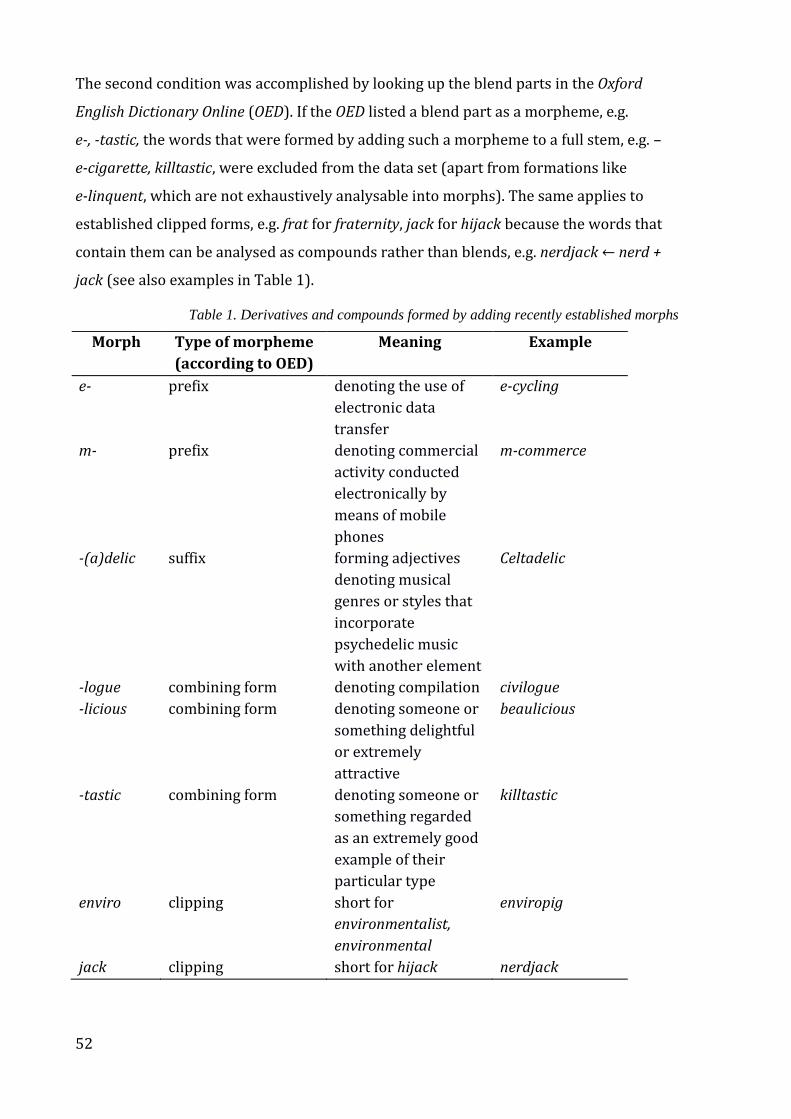
52

The second condition was accomplished by looking up the blend parts in the Oxford

English Dictionary Online (OED). If the OED listed a blend part as a morpheme, e.g.

e-, -tastic, the words that were formed by adding such a morpheme to a full stem, e.g. –

e-cigarette, killtastic, were excluded from the data set (apart from formations like

e-linquent, which are not exhaustively analysable into morphs). The same applies to

established clipped forms, e.g. frat for fraternity, jack for hijack because the words that

contain them can be analysed as compounds rather than blends, e.g. nerdjack ← nerd +

jack (see also examples in Table 1).

Table 1. Derivatives and compounds formed by adding recently established morphs

Morph Type of morpheme

(according to OED)

Meaning Example

e- prefix denoting the use of

electronic data

transfer

e-cycling

m- prefix denoting commercial

activity conducted

electronically by

means of mobile

phones

m-commerce

-(a)delic suffix forming adjectives

denoting musical

genres or styles that

incorporate

psychedelic music

with another element

Celtadelic

-logue combining form denoting compilation civilogue

-licious combining form denoting someone or

something delightful

or extremely

attractive

beaulicious

-tastic combining form denoting someone or

something regarded

as an extremely good

example of their

particular type

killtastic

enviro clipping short for

environmentalist,

environmental

enviropig

jack clipping short for hijack nerdjack

http://english.oxforddictionaries.com/view/

















53

Defining the number of source forms of a particular blend sometimes required a wider

context than just the morphological constituents. Thus, on-call-ogist can be analysed as a

three-constituent blend, i.e. on + call + oncologist, but it is obvious from the context in

which it appears, shown in (4.1), that it is a blend of on call and oncologist, and, therefore

has two source forms, as the majority of the blends do. On the other hand,

Thankshallowistmas ← Thanksgiving + Halloween + Christmas is definitely a three-part

blend.

(4.1) She looked at me, her eyebrows twisted. "Yeah, I'm on call three times a week."

"Doesn't that mean you're an on-call-ogist?" (McFedries 2011)

Using these methods, 506 neologisms were collected, among which 415 nouns, 50

adjectives, 39 verbs and 2 adverbs (the full list is given in Appendix 1). Out of those, 15

words can be analysed as either nouns or verbs (e.g. dweet / to dweet ← drunk + tweet /

drink + tweet) and 6 as either nouns or adjectives (e.g. cinematard ← cinema + retard). In

each case a category ambiguous word was assigned to one of the categories according to

the use in the sources the word was found in, or, if usage in both categories was attested,

to the category which corresponded to the majority of the examples that could be found.

The vast majority of the data are two-constituent formations, 8 are three-constituent,

and 4 are four-constituent.

There are parts of blends, which, although not listed in the OED as combining forms,

clipped forms or other kinds of morphemes, seem to demonstrate a certain productivity,

as they appear in more than one blend either in the present collection or in COCA. For

example, two blends in our data have the final part -coustic: elecoustic, funkcoustic; the

COCA search provides 10 words ending in -zilla: bridezilla, groomzilla, etc. The forms

like -coustic or -zilla are what Lehrer (1996, p. 361) calls ‘independent bound

morphemes’, or what in other sources (e.g. Bauer 2006; Bauer et al. 2013) are referred

to as splinters which are used productively in more than one word. Overall, 25 initial

and 52 final splinters in the data set can be regarded as productive to a greater or lesser

extent. They appear in 150 blends in total, which comprises a little over 28% of the data.

Excluding such words from the corpus of blends would mean taking a somewhat

extreme approach and stating that the only formations that can be classified as blends

are those that merge their source words in a unique way so that the same splinter has

never been used to form other words. A classification of this kind would risk the

establishment of a maze of categories even more ill-defined than the one I aim to pin

54

down. Moreover, in the course of data analysis, whatever method was used (see below),

the fact that a splinter could be found in one blend or in more than one did not appear to

be a factor that influenced the form of the blend. Therefore, blends with productive

splinters remain in the corpus. Their presence shows that, given appropriate conditions,

a part of a blend may undergo a gradual process of turning into a productive splinter

and eventually into a morpheme. The conditions that determine the productivity are

outside the scope of this study, but the fact that this process takes place is another

reason to focus on relatively novel blends.

To get a better understanding of how exactly the source forms are merged into blends,

their phonological, structural, and semantic properties were considered. The phonemic

transcriptions of the source words for all the blends were acquired from Cambridge

English Pronouncing Dictionary (CEPD). For obvious reasons, the transcriptions of the

blends themselves could not be found in any dictionaries, and not all the sources gave

transcriptions. If the source provided a transcription of the blend, it was brought into

compliance with the notation of CEPD. If no transcription of the blend was provided, it

was compiled from the transcriptions of the source words, in which case the country of

the blend’s origin was born in mind and the corresponding variant of transcription was

chosen, e.g. the US English transcription /kwɑːn.zə/ for Kwanzaa and /ˈræm.ə.dɑn/ for

Ramadan in a Northern American origin blend Christmahanukkwanzadan. In the

presentation of American transcriptions, the superscript for sounded r was omitted for

simplicity reasons, e.g. /ə/ instead of /ər/ is recorded. Quality changes of the sounds

were taken into consideration when deciding which phonemes were preserved in the

blends and which not. For example, even though on the graphical level all but one of the

letters of the word mascara are preserved in the blend mascary ← mascara + scary, on

the phonological level only /mæsˈk/ of /mæsˈkɑː.rə/ is preserved in /mæ'skeə.ri/,

because the stressed vowel comes from the second source word scary. Therefore, the

lengths of splinters and the degree of overlap for some of the blends are different

depending on whether graphemes or phonemes are the basis of the analysis.

For the purposes of computational analysis all transcriptions were re-coded using the

adapted version of the Speech Assessment Methods Phonetic Alphabet (SAMPA) (Wells

1997) based on IPA. The statistical analysis of the data was performed using R software

package (R Development Core Team 2012). For various steps of data analysis different

55

statistical methods were used, and a description of each particular method will follow

below where appropriate.

It is widely accepted (e.g. Cannon 1986; Renner 2006; Brdar-Szabó and Brdar 2008) that

the majority of blends combine the initial part of the first source word (W1) with the

final part of the second source word (W2); in terms of the formula from Plag (2003, p.

123):

(4.2) AB + CD = AD

The formula in (4.2) does not provide sufficient elements to deal with all the data

collected, particularly when more than two source words were involved. As a result of

applying the logic of Plag’s formula to the lexical data, depending on how many source

words took part in the formation and what parts of the source words were preserved,

new labels for structural types were created, as shown in (4.3). The parts of the source

words that do not enter blends are put in parentheses.

(4.3)

a) AB + CD = AC: for initial-initial splinter formations, e.g. hydrail ← hydr(ogen) +

rail(way)

b) AB + CD + EF (+ GH) = (X): for three- or four-constituent blends, e.g. SoLoMo ←

so(cial) + lo(cal) + mo(bile) (ACE), bastitcherbator ← bast(ard) +( b)itch +

(mast)urbator (ADF), afflufemza ← afflu(ent) + fem(inist) + m(others) + (influen)za

(ACEH)

The labelling system had also to account for cases of full preservation of one or more of

the source words, as in alcoholimia ← alcohol + (bu)limia. As a result, all the collected

neologisms were classified into structural types as illustrated in Table 2:

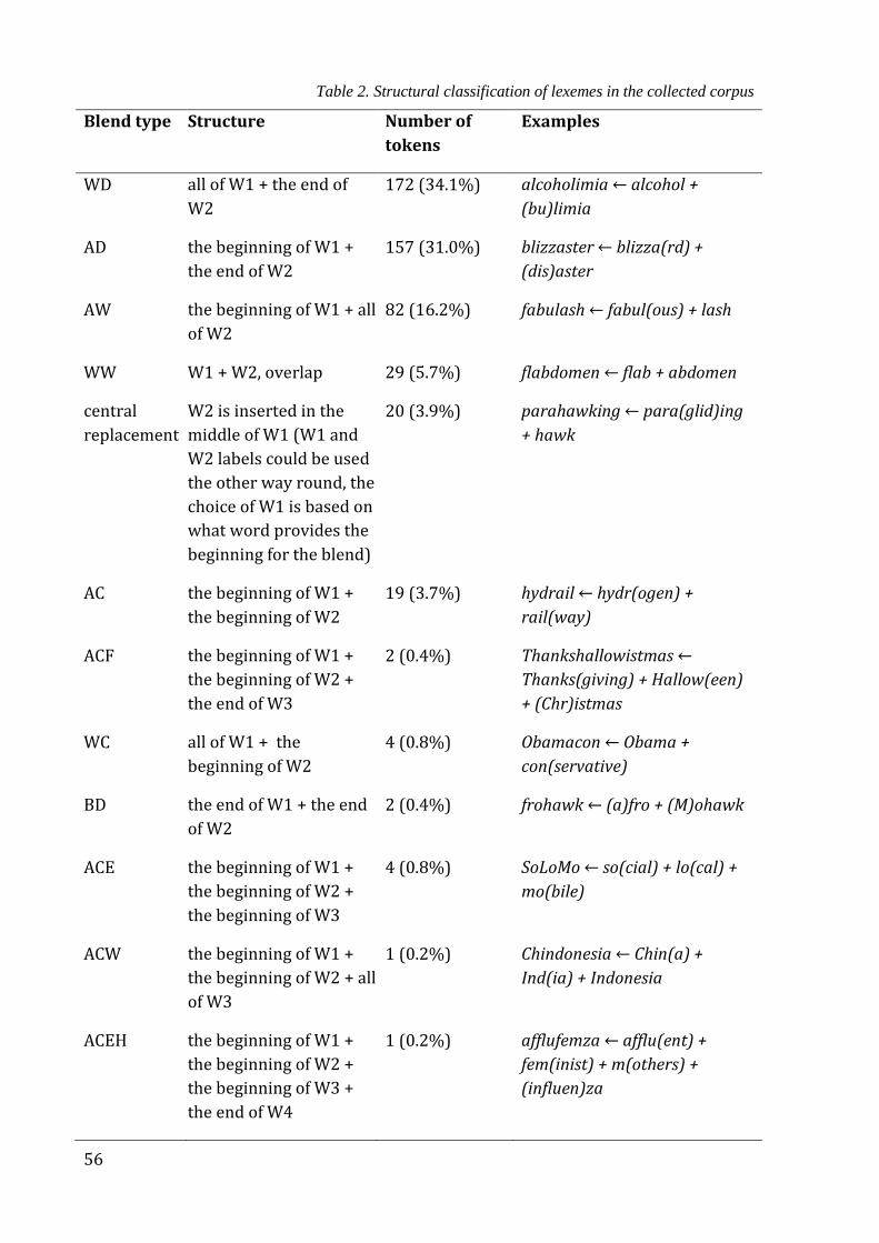
56

Table 2. Structural classification of lexemes in the collected corpus

Blend type Structure Number of

tokens

Examples

WD all of W1 + the end of

W2

172 (34.1%) alcoholimia ← alcohol +

(bu)limia

AD the beginning of W1 +

the end of W2

157 (31.0%) blizzaster ← blizza(rd) +

(dis)aster

AW the beginning of W1 + all

of W2

82 (16.2%) fabulash ← fabul(ous) + lash

WW W1 + W2, overlap 29 (5.7%) flabdomen ← flab + abdomen

central

replacement

W2 is inserted in the

middle of W1 (W1 and

W2 labels could be used

the other way round, the

choice of W1 is based on

what word provides the

beginning for the blend)

20 (3.9%) parahawking ← para(glid)ing

+ hawk

AC the beginning of W1 +

the beginning of W2

19 (3.7%) hydrail ← hydr(ogen) +

rail(way)

ACF the beginning of W1 +

the beginning of W2 +

the end of W3

2 (0.4%) Thankshallowistmas ←

Thanks(giving) + Hallow(een)

+ (Chr)istmas

WC all of W1 + the

beginning of W2

4 (0.8%) Obamacon ← Obama +

con(servative)

BD the end of W1 + the end

of W2

2 (0.4%) frohawk ← (a)fro + (M)ohawk

ACE the beginning of W1 +


the beginning of W3

4 (0.8%) SoLoMo ← so(cial) + lo(cal) +

mo(bile)

ACW the beginning of W1 +

the beginning of W2 + all

of W3

1 (0.2%) Chindonesia ← Chin(a) +

Ind(ia) + Indonesia

ACEH the beginning of W1 +



the end of W4

1 (0.2%) afflufemza ← afflu(ent) +

fem(inist) + m(others) +

(influen)za

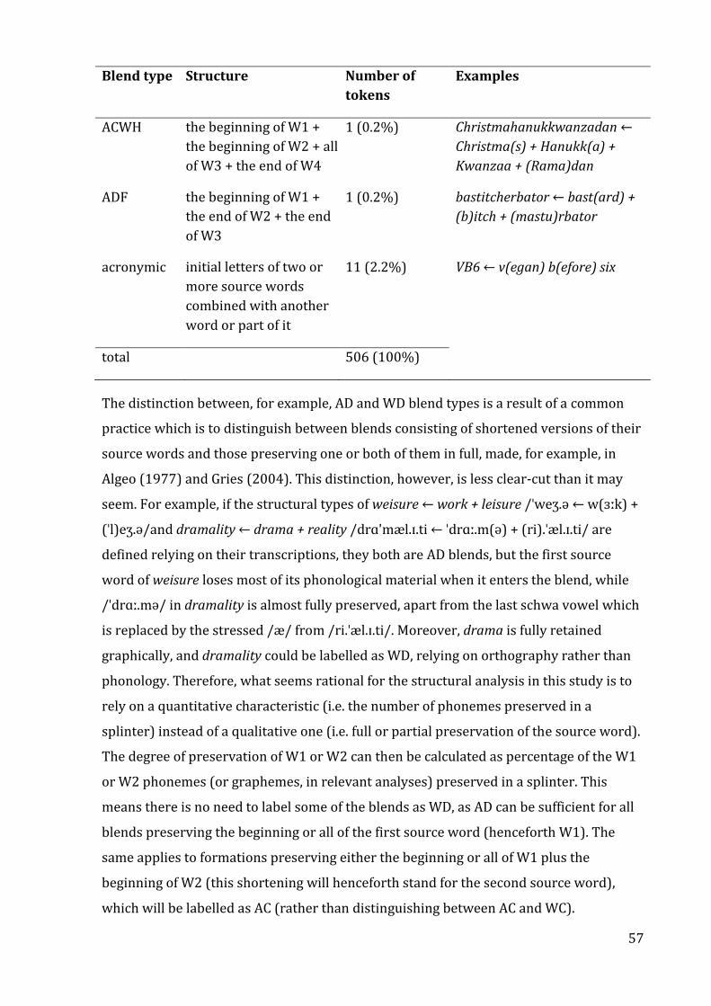
57


tokens

Examples

ACWH the beginning of W1 +

the beginning of W2 + all

of W3 + the end of W4

1 (0.2%) Christmahanukkwanzadan ←

Christma(s) + Hanukk(a) +

Kwanzaa + (Rama)dan

ADF the beginning of W1 +

the end of W2 + the end

of W3

1 (0.2%) bastitcherbator ← bast(ard) +

(b)itch + (mastu)rbator

acronymic initial letters of two or

more source words

combined with another

word or part of it

11 (2.2%) VB6 ← v(egan) b(efore) six

total 506 (100%)

The distinction between, for example, AD and WD blend types is a result of a common

practice which is to distinguish between blends consisting of shortened versions of their

source words and those preserving one or both of them in full, made, for example, in

Algeo (1977) and Gries (2004). This distinction, however, is less clear-cut than it may

seem. For example, if the structural types of weisure ← work + leisure /ˈweʒ.ə ← w(ɜːk) +

(ˈl)eʒ.ə/and dramality ← drama + reality /drɑ'mæl.ɪ.ti ← ˈdrɑː.m(ə) + (ri).ˈæl.ɪ.ti/ are

defined relying on their transcriptions, they both are AD blends, but the first source

word of weisure loses most of its phonological material when it enters the blend, while

/ˈdrɑː.mə/ in dramality is almost fully preserved, apart from the last schwa vowel which

is replaced by the stressed /æ/ from /ri.ˈæl.ɪ.ti/. Moreover, drama is fully retained

graphically, and dramality could be labelled as WD, relying on orthography rather than

phonology. Therefore, what seems rational for the structural analysis in this study is to

rely on a quantitative characteristic (i.e. the number of phonemes preserved in a

splinter) instead of a qualitative one (i.e. full or partial preservation of the source word).

The degree of preservation of W1 or W2 can then be calculated as percentage of the W1

or W2 phonemes (or graphemes, in relevant analyses) preserved in a splinter. This

means there is no need to label some of the blends as WD, as AD can be sufficient for all

blends preserving the beginning or all of the first source word (henceforth W1). The

same applies to formations preserving either the beginning or all of W1 plus the

beginning of W2 (this shortening will henceforth stand for the second source word),

which will be labelled as AC (rather than distinguishing between AC and WC).

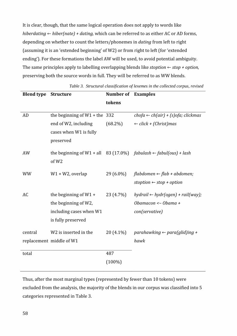
58

It is clear, though, that the same logical operation does not apply to words like

hiberdating ← hiber(nate) + dating, which can be referred to as either AC or AD forms,

depending on whether to count the letters/phonemes in dating from left to right

(assuming it is an ‘extended beginning’ of W2) or from right to left (for ‘extended

ending’). For these formations the label AW will be used, to avoid potential ambiguity.

The same principles apply to labelling overlapping blends like stoption ← stop + option,

preserving both the source words in full. They will be referred to as WW blends.

Table 3. Structural classification of lexemes in the collected corpus, revised


tokens

Examples

AD the beginning of W1 + the

end of W2, including

cases when W1 is fully

preserved

332

(68.2%)

chofa ← ch(air) + (s)ofa; clickmas

← click + (Christ)mas

AW the beginning of W1 + all

of W2

83 (17.0%) fabulash ← fabul(ous) + lash

WW W1 + W2, overlap 29 (6.0%) flabdomen ← flab + abdomen;

stoption ← stop + option

AC the beginning of W1 +

the beginning of W2,

including cases when W1

is fully preserved

23 (4.7%) hydrail ← hydr(ogen) + rail(way);

Obamacon <– Obama +

con(servative)

central

replacement

W2 is inserted in the

middle of W1

20 (4.1%) parahawking ← para(glid)ing +

hawk

total 487

(100%)

Thus, after the most marginal types (represented by fewer than 10 tokens) were

excluded from the analysis, the majority of the blends in our corpus was classified into 5

categories represented in Table 3.

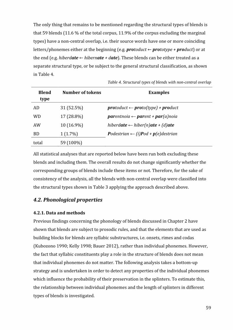
59

The only thing that remains to be mentioned regarding the structural types of blends is

that 59 blends (11.6 % of the total corpus, 11.9% of the corpus excluding the marginal

types) have a non-central overlap, i.e. their source words have one or more coinciding

letters/phonemes either at the beginning (e.g. protoduct ← prototype + product) or at

the end (e.g. hiberdate ← hibernate + date). These blends can be either treated as a

separate structural type, or be subject to the general structural classification, as shown

in Table 4.

Table 4. Structural types of blends with non-central overlap

Blend

type

Number of tokens Examples

AD 31 (52.5%) protoduct ← proto(type) + product

WD 17 (28.8%) parentnoia ← parent + par(a)noia

AW 10 (16.9%) hiberdate ← hiber(n)ate + (d)ate

BD 1 (1.7%) Podestrian ← (i)Pod + p(e)destrian

total 59 (100%)

All statistical analyses that are reported below have been run both excluding these

blends and including them. The overall results do not change significantly whether the

corresponding groups of blends include these items or not. Therefore, for the sake of

consistency of the analysis, all the blends with non-central overlap were classified into

the structural types shown in Table 3 applying the approach described above.

4.2. Phonological properties

4.2.1. Data and methods

Previous findings concerning the phonology of blends discussed in Chapter 2 have

shown that blends are subject to prosodic rules, and that the elements that are used as

building blocks for blends are syllabic substructures, i.e. onsets, rimes and codas

(Kubozono 1990; Kelly 1998; Bauer 2012), rather than individual phonemes. However,

the fact that syllabic constituents play a role in the structure of blends does not mean

that individual phonemes do not matter. The following analysis takes a bottom-up

strategy and is undertaken in order to detect any properties of the individual phonemes

which influence the probability of their preservation in the splinters. To estimate this,

the relationship between individual phonemes and the length of splinters in different

types of blends is investigated.

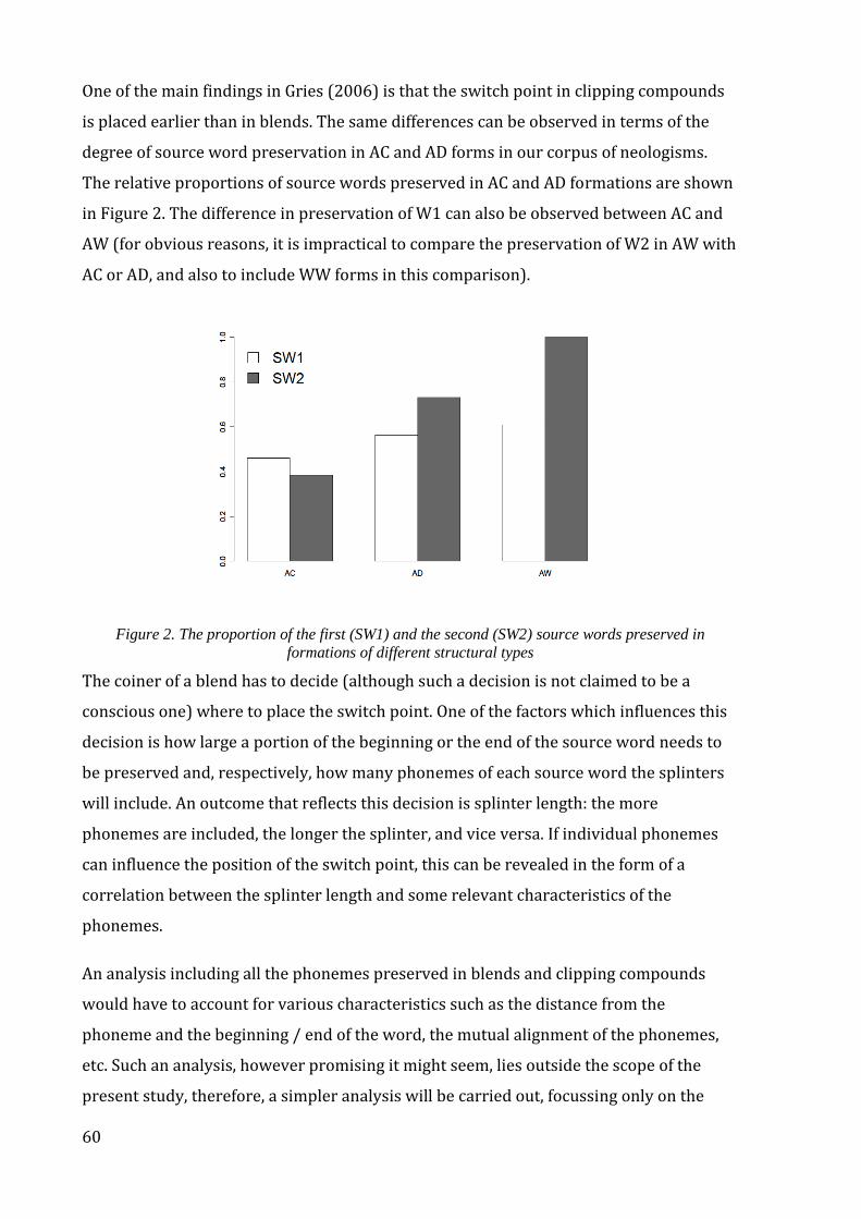
60

One of the main findings in Gries (2006) is that the switch point in clipping compounds

is placed earlier than in blends. The same differences can be observed in terms of the

degree of source word preservation in AC and AD forms in our corpus of neologisms.

The relative proportions of source words preserved in AC and AD formations are shown

in Figure 2. The difference in preservation of W1 can also be observed between AC and

AW (for obvious reasons, it is impractical to compare the preservation of W2 in AW with

AC or AD, and also to include WW forms in this comparison).

Figure 2. The proportion of the first (SW1) and the second (SW2) source words preserved in

formations of different structural types

The coiner of a blend has to decide (although such a decision is not claimed to be a

conscious one) where to place the switch point. One of the factors which influences this

decision is how large a portion of the beginning or the end of the source word needs to

be preserved and, respectively, how many phonemes of each source word the splinters

will include. An outcome that reflects this decision is splinter length: the more

phonemes are included, the longer the splinter, and vice versa. If individual phonemes

can influence the position of the switch point, this can be revealed in the form of a

correlation between the splinter length and some relevant characteristics of the

phonemes.

An analysis including all the phonemes preserved in blends and clipping compounds

would have to account for various characteristics such as the distance from the

phoneme and the beginning / end of the word, the mutual alignment of the phonemes,

etc. Such an analysis, however promising it might seem, lies outside the scope of the

present study, therefore, a simpler analysis will be carried out, focussing only on the

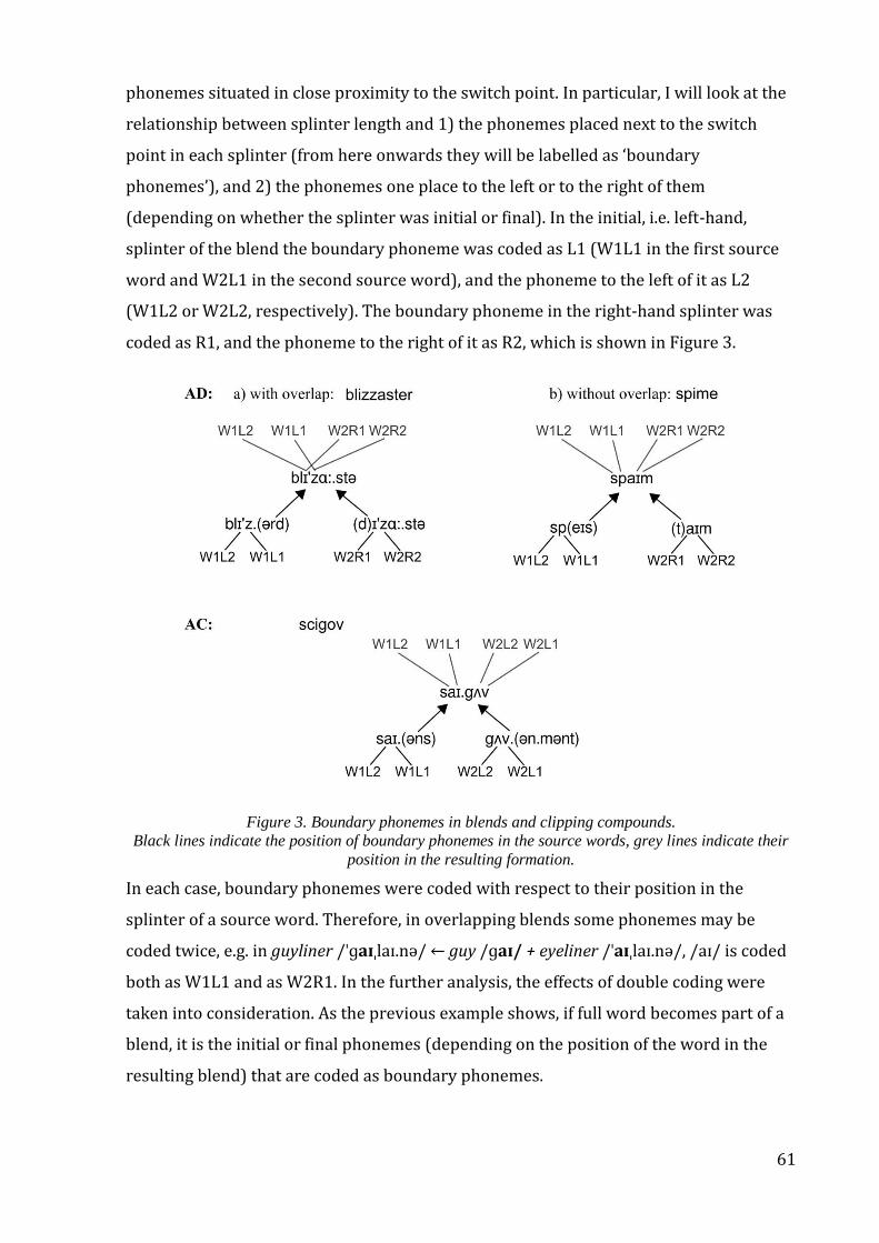
61

phonemes situated in close proximity to the switch point. In particular, I will look at the

relationship between splinter length and 1) the phonemes placed next to the switch

point in each splinter (from here onwards they will be labelled as ‘boundary

phonemes’), and 2) the phonemes one place to the left or to the right of them

(depending on whether the splinter was initial or final). In the initial, i.e. left-hand,

splinter of the blend the boundary phoneme was coded as L1 (W1L1 in the first source

word and W2L1 in the second source word), and the phoneme to the left of it as L2

(W1L2 or W2L2, respectively). The boundary phoneme in the right-hand splinter was

coded as R1, and the phoneme to the right of it as R2, which is shown in Figure 3.

Figure 3. Boundary phonemes in blends and clipping compounds.

Black lines indicate the position of boundary phonemes in the source words, grey lines indicate their

position in the resulting formation.

In each case, boundary phonemes were coded with respect to their position in the

splinter of a source word. Therefore, in overlapping blends some phonemes may be

coded twice, e.g. in guyliner /ˈɡaɪˌlaɪ.nə/ ← guy /ɡaɪ/ + eyeliner /ˈaɪˌlaɪ.nə/, /aɪ/ is coded

both as W1L1 and as W2R1. In the further analysis, the effects of double coding were

taken into consideration. As the previous example shows, if full word becomes part of a

blend, it is the initial or final phonemes (depending on the position of the word in the

resulting blend) that are coded as boundary phonemes.

62

The purpose of the analysis is to figure out whether there is any association between the

length of the splinter and the ranking of any of the two phonemes in close proximity to

the switch point (accounting also for the fact that longer splinters may come from longer

source words). The analysis included pairwise correlations between W1 and W2

splinter length and: 1) whole blend length, 2) source word length, 3) sonority/frequency

ranks of boundary phonemes.

The sonority ranking was adapted from Giegerich (1992, p. 152), grading from the most

sonorant low vowels to voiceless stops with minimal sonority. As for frequency ranking,

two methods were used. Firstly, the relative token frequencies of phonemes were

adapted from Mines et al. (1978) who used a database containing 103,887 phoneme

occurrences taken from casual conversational American English obtained from recorded

interviews. In addition to that, the frequency with which each phoneme appeared in the

current data set was calculated. All the frequency-based analyses (see below) showed

similar results with both measures of frequency.

It is important to note that the labels for the structural types (AC, AD and others) will

not be used as variables in any of the simple correlation analyses. The terms ‘initial

/final splinter’ and ‘left /right splinter’ mentioned interchangeably in section 4.2.2

reflect the position of the splinter in the source word, not in the resultant formation.

Therefore, the terms ‘initial splinter’ or ‘left splinter’ refer to the A part of AC, AD, and

AW forms, as well as the C part of the AC forms. Likewise, the terms ‘final splinter’ or

‘right splinter’ refer to the D part of AD forms, the W part of AW forms, and the right part

of the WW forms.

4.2.2. Results and discussion

The correlation analysis shows that both the initial and the final splinter lengths are

related to:

1) the length of the whole blend,

2) the source word lengths, and

3) the sonority and frequency ranks of the boundary phonemes.

Both W1 left splinter length and W2 right splinter length are positively correlated with

the length of the whole blend (r=0.64, p<0.001 for the correlation between blend length

and the length of the left splinter, r=0.48, p<0.001 for the correlation between blend

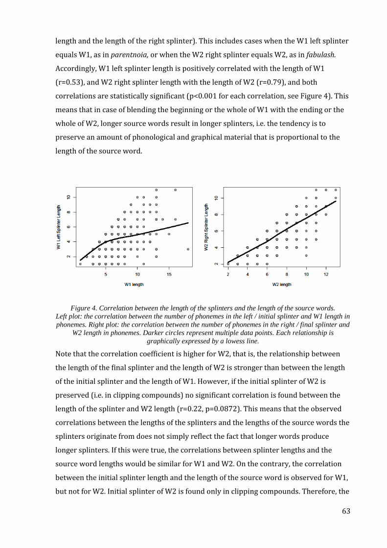
63

length and the length of the right splinter). This includes cases when the W1 left splinter

equals W1, as in parentnoia, or when the W2 right splinter equals W2, as in fabulash.

Accordingly, W1 left splinter length is positively correlated with the length of W1

(r=0.53), and W2 right splinter length with the length of W2 (r=0.79), and both

correlations are statistically significant (p<0.001 for each correlation, see Figure 4). This

means that in case of blending the beginning or the whole of W1 with the ending or the

whole of W2, longer source words result in longer splinters, i.e. the tendency is to

preserve an amount of phonological and graphical material that is proportional to the

length of the source word.

Figure 4. Correlation between the length of the splinters and the length of the source words.

Left plot: the correlation between the number of phonemes in the left / initial splinter and W1 length in

phonemes. Right plot: the correlation between the number of phonemes in the right / final splinter and

W2 length in phonemes. Darker circles represent multiple data points. Each relationship is

graphically expressed by a lowess line.

Note that the correlation coefficient is higher for W2, that is, the relationship between

the length of the final splinter and the length of W2 is stronger than between the length

of the initial splinter and the length of W1. However, if the initial splinter of W2 is

preserved (i.e. in clipping compounds) no significant correlation is found between the

length of the splinter and W2 length (r=0.22, p=0.0872). This means that the observed

correlations between the lengths of the splinters and the lengths of the source words the

splinters originate from does not simply reflect the fact that longer words produce

longer splinters. If this were true, the correlations between splinter lengths and the

source word lengths would be similar for W1 and W2. On the contrary, the correlation

between the initial splinter length and the length of the source word is observed for W1,

but not for W2. Initial splinter of W2 is found only in clipping compounds. Therefore, the

64

observed difference indicates that the splinters of AC-forms are shortened with less

regard to how much of the source word is retained than the splinters of other forms in

the present collection. Such a conclusion, however, has to be treated with caution

because the absence of the correlation between W2 initial splinter length and the length

of W2 may be due to low number of observations (only 23 AC formations in the collected

data set).

The relations between the splinter length and the ranking of the boundary phonemes

depend on whether the splinter is initial (left) or final (right). The correlation between

the length of the left splinter and the sonority of the boundary phonemes turned out to

be close to zero (rs=0, p=0.928 for the correlation between the length of the left splinter

and W1L1 sonority, rs=-0.08, p=0.0894 for the correlation between the length of the left

splinter and W1L2 sonority, rs stands for Spearman’s correlation coefficient, which is

used here and below when dealing with ranked data). This means that the sonority of

the phonemes in the data has no effect on the probability of them being included in the

initial splinter. There is, however, a weak correlation between the sonority rank of the

boundary phonemes in the right splinter and the right splinter length (rs=0.1, p=0.0345

for the correlation between the length of the right splinter and W2R1 sonority, rs=-0.26,

p<0.001 for the correlation between the length of the right splinter and W2R2 sonority).

The analysis also shows a moderate correlation between the sonority of the boundary

phonemes themselves (rs=-0.35, p<0.001 for the correlation between W1L1 and W2L2

in the left splinter, and rs=-0.51, p<0.001 for the correlation between W2R1 and W2R2

in the right splinter, rs=0.12, p<0.001 for the correlation between W1L1 and W2R1 at

the switch point of AD-formations). This suggests that the neighbouring sounds are not

independent of each other, and confirms that blends are subject to phonotactic

constraints, which in itself is not an unexpected finding.

The correlation between the sonority of neighbouring phonemes can be explained by

phonotactic constraints that operate for any words, not necessarily blends. Thus, the

sonority of a syllable gradually rises from the onset to the peak, and then gradually fades

into the coda (see, for example, Giegerich (1992) for a discussion of phonotactic

constraints in English). This means that the sonority ranks of any neighbouring

phonemes in a word are related, hence the above result. The observed correlation

between the sonorities of W1L1 and W2R1 reflects the fact that the left splinter of W1 is

often merged with the right splinter of W2 at the boundaries of syllable constituents

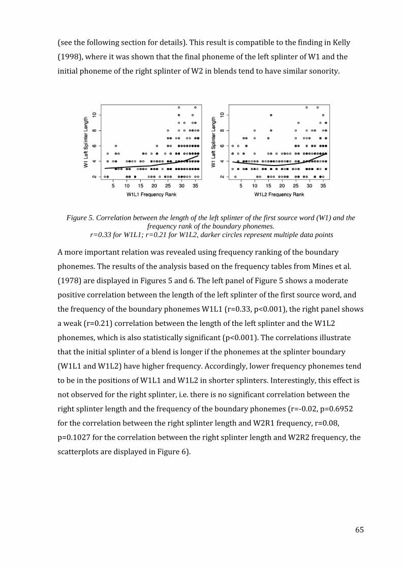
65

(see the following section for details). This result is compatible to the finding in Kelly

(1998), where it was shown that the final phoneme of the left splinter of W1 and the

initial phoneme of the right splinter of W2 in blends tend to have similar sonority.

Figure 5. Correlation between the length of the left splinter of the first source word (W1) and the

frequency rank of the boundary phonemes.

r=0.33 for W1L1; r=0.21 for W1L2, darker circles represent multiple data points

A more important relation was revealed using frequency ranking of the boundary

phonemes. The results of the analysis based on the frequency tables from Mines et al.

(1978) are displayed in Figures 5 and 6. The left panel of Figure 5 shows a moderate

positive correlation between the length of the left splinter of the first source word, and

the frequency of the boundary phonemes W1L1 (r=0.33, p<0.001), the right panel shows

a weak (r=0.21) correlation between the length of the left splinter and the W1L2

phonemes, which is also statistically significant (p<0.001). The correlations illustrate

that the initial splinter of a blend is longer if the phonemes at the splinter boundary

(W1L1 and W1L2) have higher frequency. Accordingly, lower frequency phonemes tend

to be in the positions of W1L1 and W1L2 in shorter splinters. Interestingly, this effect is

not observed for the right splinter, i.e. there is no significant correlation between the

right splinter length and the frequency of the boundary phonemes (r=-0.02, p=0.6952

for the correlation between the right splinter length and W2R1 frequency, r=0.08,

p=0.1027 for the correlation between the right splinter length and W2R2 frequency, the

scatterplots are displayed in Figure 6).

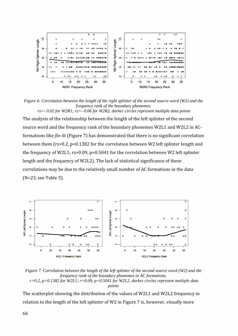
66

Figure 6. Correlation between the length of the right splinter of the second source word (W2) and the

frequency rank of the boundary phonemes.

rs=- 0.02 for W2R1; rs=- 0.06 for W2R2, darker circles represent multiple data points

The analysis of the relationship between the length of the left splinter of the second

source word and the frequency rank of the boundary phonemes W2L1 and W2L2 in AC-

formations like fin-lit (Figure 7) has demonstrated that there is no significant correlation

between them (rs=0.2, p=0.1382 for the correlation between W2 left splinter length and

the frequency of W2L1; rs=0.09, p=0.5041 for the correlation between W2 left splinter

length and the frequency of W2L2). The lack of statistical significance of these

correlations may be due to the relatively small number of AC formations in the data

(N=23, see Table 3).

Figure 7. Correlation between the length of the left splinter of the second source word (W2) and the

frequency rank of the boundary phonemes in AC formations.

r=0.2, p=0.1382 for W2L1; r=0.09, p=0.5041 for W2L2, darker circles represent multiple data

points

The scatterplot showing the distribution of the values of W2L1 and W2L2 frequency in

relation to the length of the left splinter of W2 in Figure 7 is, however, visually more

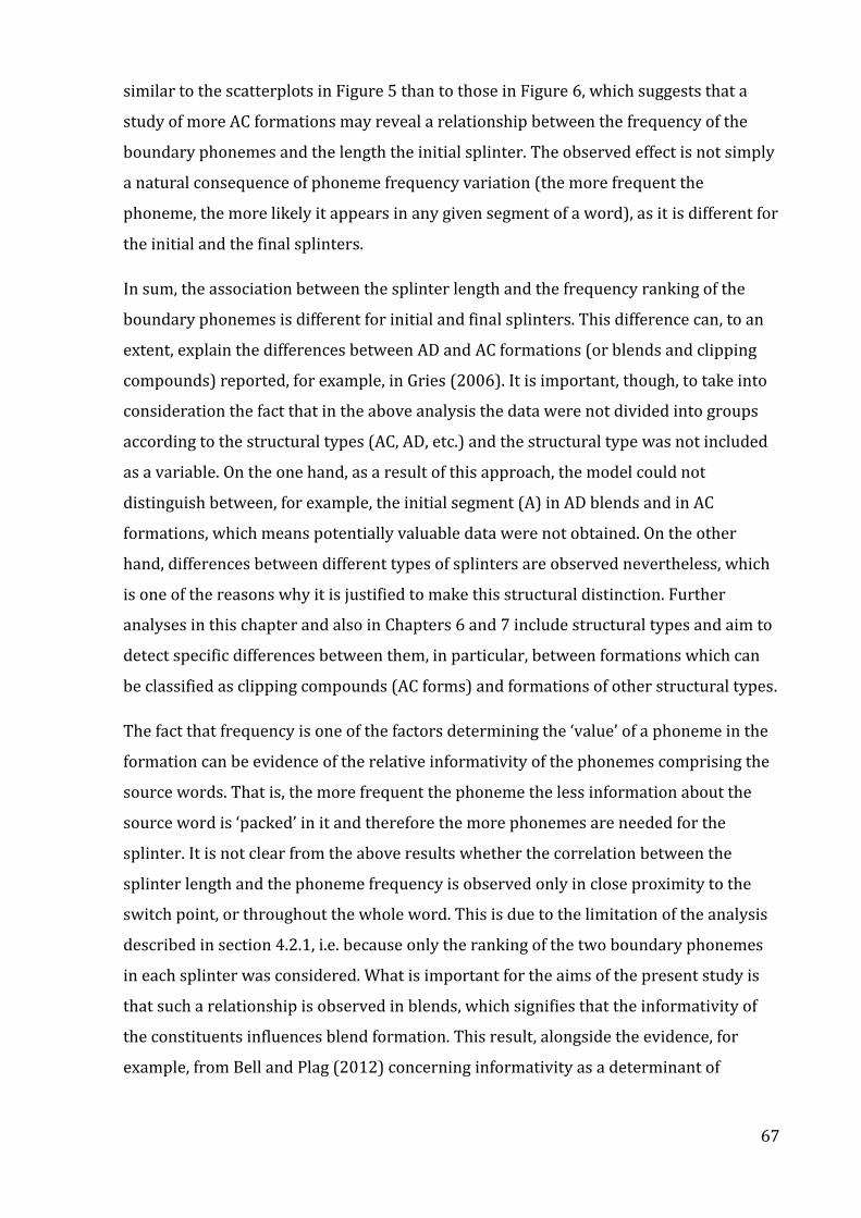
67

similar to the scatterplots in Figure 5 than to those in Figure 6, which suggests that a

study of more AC formations may reveal a relationship between the frequency of the

boundary phonemes and the length the initial splinter. The observed effect is not simply

a natural consequence of phoneme frequency variation (the more frequent the

phoneme, the more likely it appears in any given segment of a word), as it is different for

the initial and the final splinters.

In sum, the association between the splinter length and the frequency ranking of the

boundary phonemes is different for initial and final splinters. This difference can, to an

extent, explain the differences between AD and AC formations (or blends and clipping

compounds) reported, for example, in Gries (2006). It is important, though, to take into

consideration the fact that in the above analysis the data were not divided into groups

according to the structural types (AC, AD, etc.) and the structural type was not included

as a variable. On the one hand, as a result of this approach, the model could not

distinguish between, for example, the initial segment (A) in AD blends and in AC

formations, which means potentially valuable data were not obtained. On the other

hand, differences between different types of splinters are observed nevertheless, which

is one of the reasons why it is justified to make this structural distinction. Further

analyses in this chapter and also in Chapters 6 and 7 include structural types and aim to

detect specific differences between them, in particular, between formations which can

be classified as clipping compounds (AC forms) and formations of other structural types.

The fact that frequency is one of the factors determining the ‘value’ of a phoneme in the

formation can be evidence of the relative informativity of the phonemes comprising the

source words. That is, the more frequent the phoneme the less information about the

source word is ‘packed’ in it and therefore the more phonemes are needed for the

splinter. It is not clear from the above results whether the correlation between the

splinter length and the phoneme frequency is observed only in close proximity to the

switch point, or throughout the whole word. This is due to the limitation of the analysis

described in section 4.2.1, i.e. because only the ranking of the two boundary phonemes

in each splinter was considered. What is important for the aims of the present study is

that such a relationship is observed in blends, which signifies that the informativity of

the constituents influences blend formation. This result, alongside the evidence, for

example, from Bell and Plag (2012) concerning informativity as a determinant of

68

compound stress, signifies that informativity may work on different levels of word

formation.

It is clear that the frequency of the separate phonemes is not the only factor determining

the switch point position in a blend: earlier research (e.g Kubozono, 1990; Gries, 2012;

Arndt-Lappe and Plag, 2013) has shown the value of other factors. Some of these factors

will be considered in the following section.

4.3 Structural properties: Interaction with phonology


Many studies of the phonology of blends focus on the place of the switch point in their

syllabic structure. However, the relations between structural type and prosody

(considered here narrowly in terms of syllable structure) have not been taken into

consideration. In this section the interaction between the syllable structure of the blends

(more specifically, the position of the switch point in relation to the syllable structure)

and their structural type will be discussed. It will be considered whether the syllable

structure provides grounds for taxonomic differentiation between different structural

types, in particular blends and clipping compounds (AC forms).

It is mentioned in the literature (e.g. Kelly 1998; Bauer 2012) that the switch point in

blends usually goes either on the syllable boundary or between syllabic constituents, e.g.

between onset and rime. The position of the switch point for each blend and clipping

compound in the collected corpus was determined with regard to the syllable

constituents. It has to be noted, however, than in numerous cases of phonological

overlap it is not possible to unambiguously determine the position of the switch point.

For example, it is not clear whether the overlapping segment /ɪz/ in the blend

/blɪzɑːstə/ comes from W1 /blɪzərd/ or from W2 /dɪzɑːstə/, or indeed from both. That

is to say, there is no way to decide whether the two splinters comprising the blend are

/blɪ/ + /zɑːstə/, /blɪz/ + /ɑːstə/ or /bl/ + /ɪzɑːstə/. To avoid this ambiguity, the

phonological content of the splinters and the position of the switch point is determined

with regard to all the phonemes from both of the source words that are preserved in

blends, including the overlap. In other words, if an overlap takes place there are two

possible switch points, one before and one after the overlapping segment. In case of

/blɪzɑːstə/, such an analysis results in identifying the right splinter /blɪz/ with the

switch point after /z/, and the left splinter /ɪzɑːstə/, with the switch point before /ɪ/.

69

Because of this approach to determining splinter boundaries, the position of the switch

point(s) is in most cases inseparable from the position of the overlap. Therefore, two

possible switch points are accounted for in the analysis.

Depending on whether the full syllables of each source word are preserved or not, all the

blends in the collected corpus can be divided into four groups presented in (4.4). In the

transcriptions below the parts of the source words which are not retained in blends are

in parentheses, the overlapping segments are in bold type, and the syllable boundaries

are marked with dots (if not already indicated by stress marks).

(4.4)

a) YY – whole syllables are preserved both from W1 and W2, the switch point is on

the syllable boundary: shyPod ← shy + iPod /ˈʃaɪ.pɒd ← ʃaɪ + ˈaɪ.(pɒd)/, neologasm

← neologism + orgasm /niˈɒl.ə.ɡæz.əm ← niˈɒl.ə.(dʒɪ.zəm) + (ˈɔː).ɡæz.əm/;

b) YN – whole syllables are preserved from W1 but not from W2, the switch point is

on the syllable boundary of W1, often there is an overlap, e.g. in jewtheran

/ˈdʒuː.θər.ən/, Jew /dʒuː/ is retained in its entirety, while the syllable /luː/ in

Lutheran /(ˈl)uː.θər.ən/ loses its onset;

c) NY – whole syllables are preserved from W2 but not from W1, the switch point is

on the syllable boundary of W2, often there is an overlap, e.g. in microwait

/ˈmaɪ.krəʊ.weɪt/, microwave /ˈmaɪ.krəʊ.weɪ(v)/ loses its coda, while wait /weɪt/

is retained in full;

d) NN – whole syllables are not preserved from W1 or W2, the switch point is not on

the syllable boundary of either words: chofa ← chair + sofa /ˈtʃəʊ.fə ← tʃ(eə) +

(ˈs)əʊ.fə/.

Note that the syllable boundaries for the source words were taken from CEPD and that

overlapping segments were coded twice, separately for W1 and W2. In blend formation

resyllabification often takes place, and the syllable structure changes. The four groups in

(4.4) were formed according to what syllables of the source words are (partially)

preserved in the blend, irrespective of whether they are still whole syllables in the blend

or they undergo resyllabification.

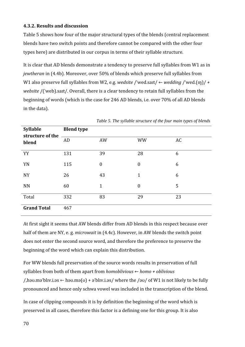
70


Table 5 shows how four of the major structural types of the blends (central replacement

blends have two switch points and therefore cannot be compared with the other four

types here) are distributed in our corpus in terms of their syllable structure.

It is clear that AD blends demonstrate a tendency to preserve full syllables from W1 as in

jewtheran in (4.4b). Moreover, over 50% of blends which preserve full syllables from

W1 also preserve full syllables from W2, e.g. wedsite /ˈwed.saɪt/ ← wedding /ˈwed.(ɪŋ)/ +

website /(ˈweb).saɪt/. Overall, there is a clear tendency to retain full syllables from the

beginning of words (which is the case for 246 AD blends, i.e. over 70% of all AD blends

in the data).

Table 5. The syllable structure of the four main types of blends

Syllable

structure of the

blend

Blend type

AD AW WW AC

YY 131 39 28 6

YN 115 0 0 6

NY 26 43 1 6

NN 60 1 0 5

Total 332 83 29 23

Grand Total 467

At first sight it seems that AW blends differ from AD blends in this respect because over

half of them are NY, e. g. microwait in (4.4c). However, in AW blends the switch point

does not enter the second source word, and therefore the preference to preserve the

beginning of the word which can explain this distribution.

For WW blends full preservation of the source words results in preservation of full

syllables from both of them apart from homoblivious ← homo + oblivious

/,həʊ.məˈblɪv.i.əs ← həʊ.mə(ʊ) + əˈblɪv.i.əs/ where the /əʊ/ of W1 is not likely to be fully

pronounced and hence only schwa vowel was included in the transcription of the blend.

In case of clipping compounds it is by definition the beginning of the word which is

preserved in all cases, therefore this factor is a defining one for this group. It is also

71

worth noting that no clear preference for any of the four situations in terms of syllable

preservation is observed for AC formations.

In the YY group, the position of the switch point is always on a syllable boundary. This

includes cases with overlap, in which both potential switch points fall onto syllable

boundaries. In YN and NY groups the switch point (or one of the two switch points, in

cases of overlap) was found in the following positions:

(4.5)

a) between onset and nucleus (119 observations), e. g. in W2 of blizzaster

/blɪˈzɑː.stə/ ← blizzard /ˈblɪz.(ərd)/ + disaster /(d)ɪˈzɑː.stə/;

b) between nucleus and coda (65 observations), e. g. both in W1 and W2 of

cheapuccino /ˌtʃiːp.ʊˈtʃiː.nəʊ/ ← cheap /tʃiːp/ + cappuccino /(ˌkæ)p.ʊˈtʃiː.nəʊ/;

c) within onset (8 observations), e. g. in W1 of awkfest /ˈɔːk.fest/ ← awkward

/ˈɔː.k(wəd)/ + fest /fest/;

d) within coda (1 observation) in W1 of frienvy /ˈfren.vi/ ← friend /fren(d)/ + envy

/ˈen.vi/.

A conditional inference tree (decision tree) analysis was performed to figure out if the

switch point placement is related to the structural type of blends. The method involves

estimating a regression relationship between the variables by binary recursive

partitioning in a conditional inference framework. In the process of building a decision

tree, the dependent variable is analysed in relation to one or several independent

variables. First, the algorithm tests the null hypothesis of independence between the

dependent variable and any of the independent variables. If the null hypothesis is

rejected, the independent variable which has the strongest association with the

dependent variable is selected. At this stage, the data is split into two groups (branches)

if the difference between the value of the outcome variable in two branches ‘growing’

from one node is statistically significant at the 5% level (that is, the p-value must be

smaller than 0.05 in order to split the node). Then this process is recursively repeated

until further splits are no longer justified. Each time the full set of independent variables

is taken into consideration for a potential node split, so that the same variable can cause

more than one split (see Hothorn et al. (2006) for a detailed description of the method).

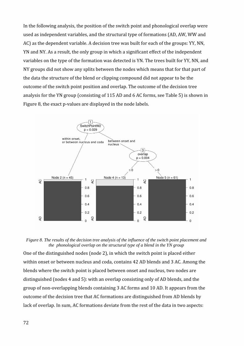
72

In the following analysis, the position of the switch point and phonological overlap were

used as independent variables, and the structural type of formations (AD, AW, WW and

AC) as the dependent variable. A decision tree was built for each of the groups: YY, NN,

YN and NY. As a result, the only group in which a significant effect of the independent

variables on the type of the formation was detected is YN. The trees built for YY, NN, and

NY groups did not show any splits between the nodes which means that for that part of

the data the structure of the blend or clipping compound did not appear to be the

outcome of the switch point position and overlap. The outcome of the decision tree

analysis for the YN group (consisting of 115 AD and 6 AC forms, see Table 5) is shown in

Figure 8, the exact p-values are displayed in the node labels.

Figure 8. The results of the decision tree analysis of the influence of the switch point placement and

the phonological overlap on the structural type of a blend in the YN group

One of the distinguished nodes (node 2), in which the switch point is placed either

within onset or between nucleus and coda, contains 42 AD blends and 3 AC. Among the

blends where the switch point is placed between onset and nucleus, two nodes are

distinguished (nodes 4 and 5): with an overlap consisting only of AD blends, and the

group of non-overlapping blends containing 3 AC forms and 10 AD. It appears from the

outcome of the decision tree that AC formations are distinguished from AD blends by

lack of overlap. In sum, AC formations deviate from the rest of the data in two aspects:

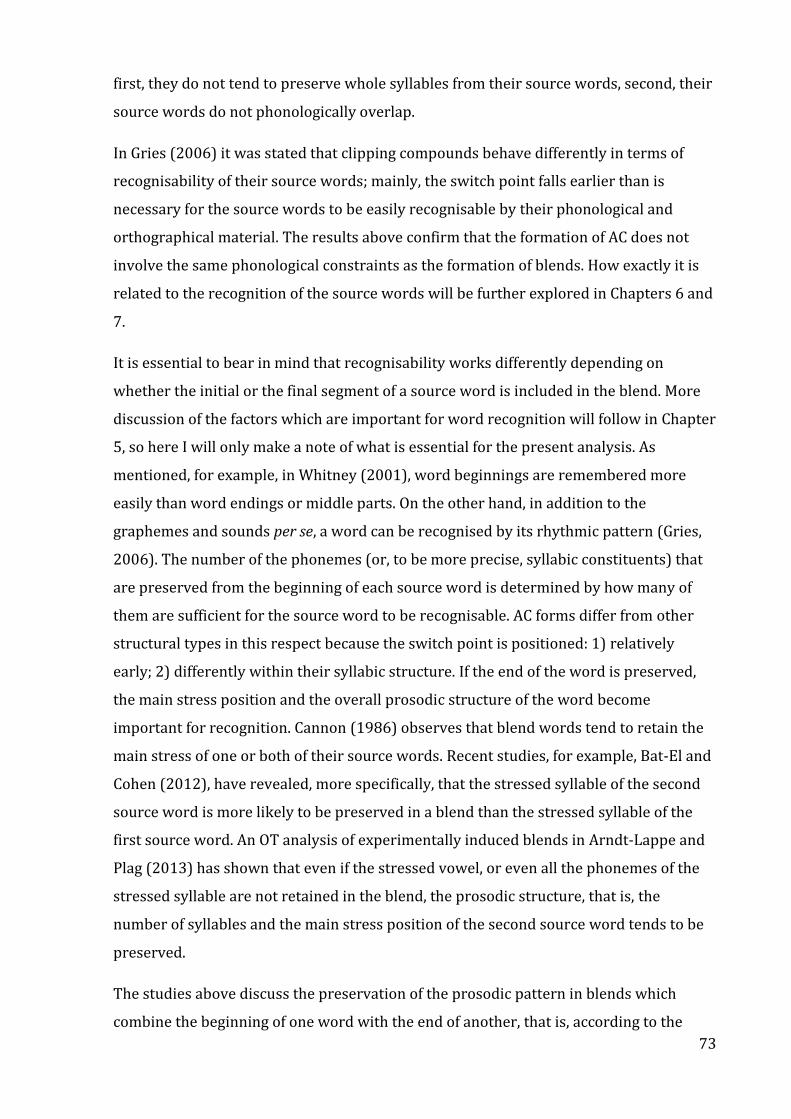
73

first, they do not tend to preserve whole syllables from their source words, second, their

source words do not phonologically overlap.

In Gries (2006) it was stated that clipping compounds behave differently in terms of

recognisability of their source words; mainly, the switch point falls earlier than is

necessary for the source words to be easily recognisable by their phonological and

orthographical material. The results above confirm that the formation of AC does not

involve the same phonological constraints as the formation of blends. How exactly it is

related to the recognition of the source words will be further explored in Chapters 6 and

7.

It is essential to bear in mind that recognisability works differently depending on

whether the initial or the final segment of a source word is included in the blend. More

discussion of the factors which are important for word recognition will follow in Chapter

5, so here I will only make a note of what is essential for the present analysis. As

mentioned, for example, in Whitney (2001), word beginnings are remembered more

easily than word endings or middle parts. On the other hand, in addition to the

graphemes and sounds per se, a word can be recognised by its rhythmic pattern (Gries,

2006). The number of the phonemes (or, to be more precise, syllabic constituents) that

are preserved from the beginning of each source word is determined by how many of

them are sufficient for the source word to be recognisable. AC forms differ from other

structural types in this respect because the switch point is positioned: 1) relatively

early; 2) differently within their syllabic structure. If the end of the word is preserved,

the main stress position and the overall prosodic structure of the word become

important for recognition. Cannon (1986) observes that blend words tend to retain the

main stress of one or both of their source words. Recent studies, for example, Bat-El and

Cohen (2012), have revealed, more specifically, that the stressed syllable of the second

source word is more likely to be preserved in a blend than the stressed syllable of the

first source word. An OT analysis of experimentally induced blends in Arndt-Lappe and

Plag (2013) has shown that even if the stressed vowel, or even all the phonemes of the

stressed syllable are not retained in the blend, the prosodic structure, that is, the

number of syllables and the main stress position of the second source word tends to be

preserved.

The studies above discuss the preservation of the prosodic pattern in blends which

combine the beginning of one word with the end of another, that is, according to the

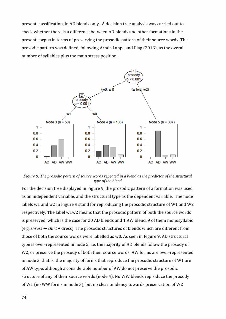
74

present classification, in AD blends only. A decision tree analysis was carried out to

check whether there is a difference between AD blends and other formations in the

present corpus in terms of preserving the prosodic pattern of their source words. The

prosodic pattern was defined, following Arndt-Lappe and Plag (2013), as the overall

number of syllables plus the main stress position.

Figure 9. The prosodic pattern of source words repeated in a blend as the predictor of the structural

type of the blend

For the decision tree displayed in Figure 9, the prosodic pattern of a formation was used

as an independent variable, and the structural type as the dependent variable. The node

labels w1 and w2 in Figure 9 stand for reproducing the prosodic structure of W1 and W2

respectively. The label w1w2 means that the prosodic pattern of both the source words

is preserved, which is the case for 20 AD blends and 1 AW blend, 9 of them monosyllabic

(e.g. shress ← shirt + dress). The prosodic structures of blends which are different from

those of both the source words were labelled as w0. As seen in Figure 9, AD structural

type is over-represented in node 5, i.e. the majority of AD blends follow the prosody of

W2, or preserve the prosody of both their source words. AW forms are over-represented

in node 3, that is, the majority of forms that reproduce the prosodic structure of W1 are

of AW type, although a considerable number of AW do not preserve the prosodic

structure of any of their source words (node 4). No WW blends reproduce the prosody

of W1 (no WW forms in node 3), but no clear tendency towards preservation of W2

75

prosody in WW can be determined either, as they are split between node 4 and node 5.

AC is the only structural type which almost categorically appears in one node (node 4),

which indicates that almost all AC forms do not follow the prosodic pattern of any of

their source words.

In sum, phonological differences between blends and clipping compounds have been

revealed at different levels: at the level of phonemes, syllable constituents, and the

word-level prosodic structure.

4.4. Semantic properties: Interaction with structure


The semantic properties of blends have often been used as the basis for their

classification according to the relationships between their source words, similar to the

classifications of compounds according to the semantic relationships between their

components, e.g. in Downing (1977), Bauer (1983), Benczes (2006) and Renner (2008).

In some cases particular semantic properties were used as distinguishing features of

blends. For example, in Adams (1973), Berg (1998), and Kelly (1998) a word is classified

as a blend (or at least as a typical blend) only if its source words are in some kind of

coordinative relation, e.g. synonymic or antonymic, or are hyponyms, otherwise it is a

clipping compound. Making this distinction seems, however, no less arbitrary then a

similar distinction based on purely formal properties of blends and clipping compounds,

as was shown in section 2.2. An integrative approach to this problem might help find

more reliable grounds for distinguishing and classifying blends. In this section, the

interaction between the form and the semantics of blends will be considered. An attempt

to make a subtle classification of semantic types and subtypes of blends is not among the

aims of the present research, therefore only two main semantic types were taken into

consideration, based on the classification from Bauer (2006):

1. paradigmatic origin blends (chofa ← chair + sofa, blizzaster ← blizzard + disaster);

2. syntagmatic origin blends (fake-ation ← fake vacation, briet ← bride diet).

These terms are synonymous to the terms ‘coordinative/determinative blends’ used, for

example, in Bauer (2012). Referring to the blends as having either paradigmatic or

syntagmatic origin implies looking at not only the semantics, but also the origin of the

blends. Paradigmatic origin blends can be glossed by linking their source words with an

76

and or or (chofa has properties of a chair and a sofa). Syntagmatic origin blends can be

glossed by modifying the second source word by the first one (e.g. briet is a bride diet, i.e.

a kind of diet). It is possible that a blend of either kind actually originates from an item-

familiar word combination of the corresponding type, but it is not necessarily the case.

Defining the semantic type of neologisms in my collection relies on the definitions and

the source words provided in the sources, and on the semantic relations between the

source words analysed in accordance with the criteria in Bauer (2006). Thus, the data

are distributed into the semantic categories in the following way: 391 formations have

syntagmatic origin, 109 have paradigmatic origin, and the remaining 6 are classified as

‘other’. The latter group includes formations which are problematic to assign to either

semantic type because the order of the source words in the explaining word

combination is reversed, as in epiphanot ← not an epiphany, or is questionable, as in

collelephant ← college + elephant, meaning ‘a large college’. Although one might argue

that the source words of collelephant are in subordinative relations, this blend is still

different from other subordinative origin blends. If we assume that it is a subordinative

blend parallel to others, this would imply that the second source word is the head word,

i.e. the meaning would be something like “an elephant with a college-like property”

which is not what the context demands.

Combinations of source words, i.e. cases of their immediate co-occurrence, were looked

up in COCA for each blend or clipping compound. Irrespective of the semantic type of the

blend or clipping compound in question, both subordinative and coordinative

combinations of its source words were looked up. The subordinative word combinations

could have only one possible word order, which was determined by the meaning of the

blend, and the coordinative word combinations could have different order of

constituents. In coordinative word combinations, the source words could be conjoined

by and or or, or could have a comma or a hyphen between them; all these variants were

looked up in the corpus.


For about one third of the data (149 of 506 lexemes) the source word combinations

could be found in COCA, and in the vast majority of cases only one type of combination

was attested, particularly, coordinative (either in direct or in reversed order, or both)

for paradigmatic origin formations, and subordinative for syntagmatic origin formations

(the exact numbers are given in Tables 6 and 7).

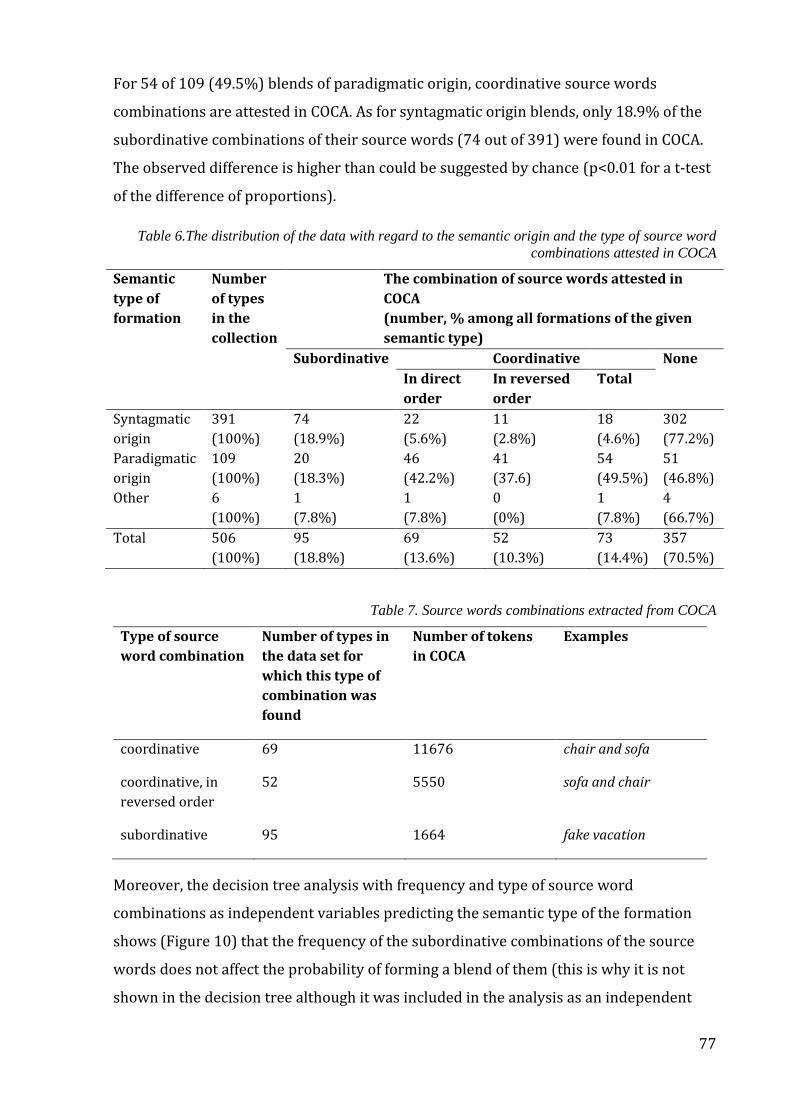
77

For 54 of 109 (49.5%) blends of paradigmatic origin, coordinative source words

combinations are attested in COCA. As for syntagmatic origin blends, only 18.9% of the

subordinative combinations of their source words (74 out of 391) were found in COCA.

The observed difference is higher than could be suggested by chance (p<0.01 for a t-test

of the difference of proportions).

Table 6.The distribution of the data with regard to the semantic origin and the type of source word

combinations attested in COCA

Semantic

type of

formation

Number

of types

in the

collection

The combination of source words attested in

COCA

(number, % among all formations of the given

semantic type)

Subordinative Coordinative None

In direct

order

In reversed

order

Total

Syntagmatic

origin

391

(100%)

74

(18.9%)

22

(5.6%)

11

(2.8%)

18

(4.6%)

302

(77.2%)

Paradigmatic

origin

109

(100%)

20

(18.3%)

46

(42.2%)

41

(37.6)

54

(49.5%)

51

(46.8%)

Other 6

(100%)

1

(7.8%)

1

(7.8%)

0

(0%)

1

(7.8%)

4

(66.7%)

Total 506

(100%)

95

(18.8%)

69

(13.6%)

52

(10.3%)

73

(14.4%)

357

(70.5%)

Table 7. Source words combinations extracted from COCA

Type of source

word combination

Number of types in

the data set for

which this type of

combination was

found

Number of tokens

in COCA

Examples

coordinative 69 11676 chair and sofa

coordinative, in

reversed order

52 5550 sofa and chair

subordinative 95 1664 fake vacation

Moreover, the decision tree analysis with frequency and type of source word

combinations as independent variables predicting the semantic type of the formation

shows (Figure 10) that the frequency of the subordinative combinations of the source

words does not affect the probability of forming a blend of them (this is why it is not

shown in the decision tree although it was included in the analysis as an independent

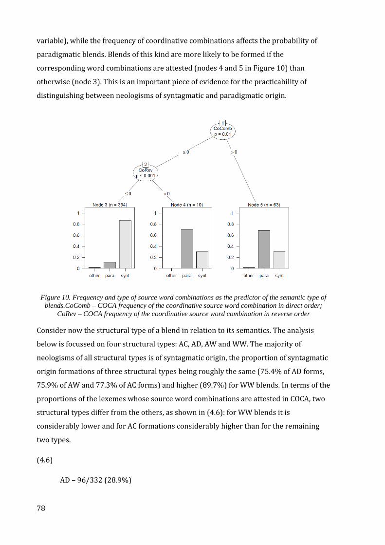
78

variable), while the frequency of coordinative combinations affects the probability of

paradigmatic blends. Blends of this kind are more likely to be formed if the

corresponding word combinations are attested (nodes 4 and 5 in Figure 10) than

otherwise (node 3). This is an important piece of evidence for the practicability of

distinguishing between neologisms of syntagmatic and paradigmatic origin.

Figure 10. Frequency and type of source word combinations as the predictor of the semantic type of

blends.CoComb – COCA frequency of the coordinative source word combination in direct order;

CoRev – COCA frequency of the coordinative source word combination in reverse order

Consider now the structural type of a blend in relation to its semantics. The analysis

below is focussed on four structural types: AC, AD, AW and WW. The majority of

neologisms of all structural types is of syntagmatic origin, the proportion of syntagmatic

origin formations of three structural types being roughly the same (75.4% of AD forms,

75.9% of AW and 77.3% of AC forms) and higher (89.7%) for WW blends. In terms of the

proportions of the lexemes whose source word combinations are attested in COCA, two

structural types differ from the others, as shown in (4.6): for WW blends it is

considerably lower and for AC formations considerably higher than for the remaining

two types.

(4.6)

AD – 96/332 (28.9%)

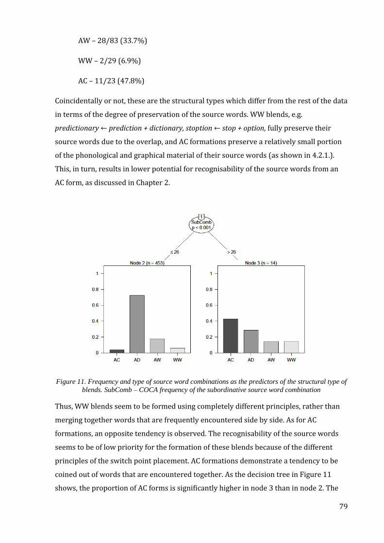
79

AW – 28/83 (33.7%)

WW – 2/29 (6.9%)

AC – 11/23 (47.8%)

Coincidentally or not, these are the structural types which differ from the rest of the data

in terms of the degree of preservation of the source words. WW blends, e.g.

predictionary ← prediction + dictionary, stoption ← stop + option, fully preserve their

source words due to the overlap, and AC formations preserve a relatively small portion

of the phonological and graphical material of their source words (as shown in 4.2.1.).

This, in turn, results in lower potential for recognisability of the source words from an

AC form, as discussed in Chapter 2.

Figure 11. Frequency and type of source word combinations as the predictors of the structural type of

blends. SubComb – COCA frequency of the subordinative source word combination

Thus, WW blends seem to be formed using completely different principles, rather than

merging together words that are frequently encountered side by side. As for AC

formations, an opposite tendency is observed. The recognisability of the source words

seems to be of low priority for the formation of these blends because of the different

principles of the switch point placement. AC formations demonstrate a tendency to be

coined out of words that are encountered together. As the decision tree in Figure 11

shows, the proportion of AC forms is significantly higher in node 3 than in node 2. The

80

subordinative source word combination frequency for node 3 is over 26, while the

frequency of the subordinative source word combinations of blends in node 3 is lower.

This means that a complex formation merging together two words is significantly more

likely to take the AC form if the frequency of the corresponding subordinative source

word combination exceeds 26. This result implies that an AC form is more likely to be

formed as a contraction of an established word combination (i.e. a clipping compound in

the sense that it is a clipping of an existing compound) than as a neologism naming a

completely new notion. The latter is, for example, the case with hybrid names such as

chofa ← chair + sofa.

If the semantic relationships between the source words are used for the classification of

blends among other morphological processes, then blends are often juxtaposed to

contractions of ‘words which occur side by side’, as formulated in Kubozono (1990, p. 2).

For example, Gries (2012, p. 155) reports evidence that ‘complex clippings have quite a

strong preference to involve contractive relations’, which means that, unlike blends,

complex clippings (AC formations here) tend to merge together words which could

appear as a compound. The analysis of the interaction of the structure of the formations

and the semantic relations between their source words shows that the structural type of

a neologism is indeed related to its actual origin.

4.5. Interim conclusions: Phonological and semantic factors which

influence the structure of blends

The coinage of blends does not employ morphemes but involves extraction of segments

of the source words and merging them together following prosodic rules, which

determine the position of the switch point. The findings described in sections 4.2–4.4

reveal the factors that influence the switch point placement: the sonority and frequency

of boundary phonemes, and the syllable structure of the source words. The correlation

between the sonority ranks of the phonemes adjacent to the switch point indicates that

blend words are formed in accordance with the phonological constraints for English

words. The positive correlation between the frequency of boundary phonemes and the

splinter length can be explained by the recognisability of the source words, which has

been shown to be an important factor in blend formation (Gries 2004, 2006, 2012). The

frequency of the phonemes, as an indirect indicator of their informativity can be related

to recognisability of the source words from the splinters in blends and clipping

compounds. This study has shown that in terms of the switch point position AC

81

formations behave differently from AD blends. Firstly, they preserve less material from

the source words than AD (or any other type of formations considered in the analysis

above). In addition to this, AC forms demonstrate a clear preference for the switch point

to be placed between onset and nucleus in the situation of no phonological overlap,

whilst AD blends do not show any preference in this respect at all. Although on the

surface (considering only the phoneme sequences) the phonology of both AD and AC

forms is similar to the phonology of other morphological categories, e.g.

monomorphemic English words, the picture becomes different if we take into

consideration the position of the switch point in the syllabic structure and the factor of

recognisability of the source words.

Another factor which must be taken into consideration in an analysis of the structure of

blends and clipping compounds is the prosodic contour of their source words. The

analysis in section 4.3 shows that whether the stress pattern of the first or the second

source word (or of none at all) is preserved, is not independent of the structural type of

the formation. The majority of AD forms preserve the prosodic pattern of the second

source words, which is compatible with earlier findings in literature. Unlike AD, AC

forms tend not to preserve the prosodic pattern of any of their source words. The fact

that AW blends tend to follow the prosodic pattern of W1 rather than W2 can be

explained by purely technical reasons. The first source word of AW blends usually has

more syllables than the second (or, to put it the other way round, W2 is fully preserved

in these blends due to the fact that it is short, usually mono- or disyllabic), e.g.

passthought ← password + thought. Therefore it is impossible for the whole blend to

reproduce the prosodic structure of the second source word. Besides, as the second

word is, by definition, fully preserved in AW blends, it ensures its recognisability and

makes its prosodic structure less important for recognition. It must be noted, however,

that a small group of AW blends, e.g. enviclean ← environment + clean do not follow these

tendencies and resemble AC formations in this respect.

It appears that two contradictory factors influence the formation of blend words. The

first is the relatively frequent co-occurrence of the source words and, therefore, the

possibility of an established semantic link between them. The second factor is the

creation of such a link simultaneously with the formation of a blend, which requires a

high degree of recognisability of both the source words. Recognisability is not so vital in

the first case because the semantic link is already there and the main aim of the

82

formation of a new lexeme is merging the source words together in a compact form. The

first factor, therefore, is responsible for producing clipping compounds, the second is

responsible for blending.

This model can explain the differences in the formation of blends and clipping

compounds. Recognisability of the source words is achieved by balancing the

preservation of the longest possible segment of both the source words (an ideal case

would be a WW blend) and the prosodic pattern of at least one of them. Which prosodic

pattern is preserved depends on the relative length of the source words and the blend,

the position of the source words (the second source word is more vulnerable if it loses

its beginning, so it is essential to preserve its prosodic pattern) as well as on which of

them is more valuable for the semantics of the blend. Thus, if one of the source words is

the semantic head, it may be the cause for the whole blend to reproduce its prosody, the

default pattern for English blends being the preservation of the second source word

prosodic pattern. The results of the experiments reported in Shaw et al. (2014) show

that, at least for blends labelled here as AD, this is indeed the case. The experiments by

Shaw et al. demonstrate that AD blends which can be analysed as right-headed tend to

preserve the prosodic pattern of the right-hand source word to a greater extent than

paradigmatic origin AD blends, which do not have a semantic head. In the present study,

this works for AD blends and the majority of AW but WW and AC forms behave

differently.

As for AC forms, recognisability seems to be a less important factor for their formation

than for AD blends. A detailed discussion of the matter and statistical evidence of the

differences between the two categories in terms of the recognisability and the similarity

of the source words is provided in Gries (2006, 2012). This study finds explanation for

these differences in the fact that AC forms originate as an instance of shortening which

often implies the existence of a frequently used combination of source words and the

existence of a certain semantic link between them prior to the formation of the new

lexeme. I tried to filter out such cases at the stage of data collection (see section 4.1), but

the analysis has shown that this might be the defining feature of AC forms.

WW blends are on the opposite end of the axis from AC forms. In WW blends, the

conditions for the recognisability of the source words are met more successfully than in

any other structural type of blends, because both words are preserved in full. The

frequent co-occurrence of the source words of these blends is, on the other hand, the

83

least probable case. A possible explanation of these features of WW blends is that they

are an instance of creative word formation introducing a new cognitive unit. To what

extent this is true, and whether this also relates to AD blends will be explored in the

following chapters.

Contrary to the claim, for example, in Tomaszewitcz (2012, p. 221) that “no relationship

between the phonological structure and syntactic origin is assumed to exist in the

English blends”, the analysis that involves AD, AW, AC and WW structural types shows

that the origin has its explanatory value. Considering the origin of a blend alongside its

structure, it is possible to distinguish two groups of AW forms, some of them likely to be

formed as blends (e.g. approximeeting), others as clipping compounds (e.g. enviclean,

see also contrail ← condensation + trail, lumist ← luminous mist in Tomaszewitcz (2012,

p. 228)), although some cases still may be debatable.

The results of this research make an important contribution to the resolution of a much

discussed problem: whether clipping compounds and blends are the same type of word

formation or not. In terms of purely formal or purely phonological features these two

groups of words demonstrate different behaviour, and the reason for this lies in their

semantic properties. AC-forms seem to appear contractions of existing compounds, and

therefore can be labelled as clipping compounds. Unlike AC-forms, other blends are

indeed more likely to be instances of creative word formation involving the formation of

new notions in the process of conceptual integration. In other circumstances, a blend of

digital and camera could be digamera, but because it was probably coined as the

shortening of already established digital camera it took the form of a clipping compound

digicam.

Going back to the different approaches to classifying blends as a word formation type

given in the Introduction, I have to note that to call blends either an instance of

shortening or an instance of compounding would be imprecise, as the process of blend

formation appears to be more complex. It is likely that blends or clipping compounds are

formed in one of two possible situations: either pure shortening takes place (in most

cases after compounding) which results in the formation of clipping compounds, or

shortening and compounding happen simultaneously. In both cases phonological rules

apply, but in the second case the output word not only has to sound like a normal

English word, but also has to preserve enough material from its source words for them

to be recognisable. This is achieved by preserving a certain amount of the phonological

84

material from the source words, as well as prosodic patterns of the appropriate source

word. This leads to a conclusion that both formal criteria that were stated in the working

definition in section 3.1 (i.e. partial loss of the phonological/graphical material and not

being formed by concatenation of morphs) are important for distinguishing blends from

the neighbouring word formation categories.

Applying these criteria to the corpus of data which was analysed in the present chapter

leads to a somewhat paradoxical conclusion: blends and clipping compounds are

definitely not the same because they have different reasons for appearing and

morphologically (if this word indeed can be applied to their formation) they are formed

according to different principles. Yet the ultimate boundary between the two categories

is impossible to draw because there are, however few, marginal cases the formation of

which may be equally successfully explained by either principle.

It has to be noted with regard to the results presented here that some of the conclusions

(in particular, the analysis of the syllable structure of the data in section 4.3) are based

on small data samples, and therefore should be treated with caution. Despite these

limitations, the results presented in this chapter provide important evidence of the

influence on the co-occurrence of constituents on the form of the output items. The

relations between the structural type of the items and the recognisability of their source

words are further explored in two experimental studies described in Chapters 6 and 7.

Some ways to provide further confirmations to the claims made here will be suggested

in the following chapter.

85

Chapter 5. Deconstructing blends: Insights from psycholinguistic and

cognitive studies

Studying phonological and structural regularities of blends and related morphological

phenomena consistently leads to the questions of 1) how blends are constructed from

the point of view of their coiners, and 2) how the readers or hearers of blends perceive

and understand them. As is clear from Chapter 2, these questions have often been raised

by researchers conducting descriptive and corpus-based studies of blends within

various theoretical frameworks. The findings of the lexical data analysis presented in

Chapter 4 also reveal that the differences between structural types of blends and

clipping compounds are related to factors involved in producing blends and to the

recognisability of the source words. It appears that it is difficult to make inferences

about the mechanism of blending without referring to psycholinguistic and cognitive

phenomena related to the formation and processing of blends. A closer look will be

taken at these in the present chapter. Section 5.1 provides an overview of studies

discussing the selection of the source words that make up potential blends, and the

semantic features of blends related to this selection. In section 5.2 the recognisability of

the source words of blends and clipping compounds is considered in the light of

psycholinguistic studies of word recognition. Section 5.3 outlines the theoretical and

methodological assumptions that are utilised for the experimental study of the

processing of blends and clipping compounds undertaken in the current research.

5.1. Cognitive mechanisms of blending revealed in the form of blends

In psycholinguistics, studies of blends were initially concerned with speech error blends

as part of the research on lapsus linguae in general. Speech error blends occur, as

proposed in Fromkin (1973b, p. 235), when two words seem to be able to express what

the speaker has in mind, and therefore the speaker “brings them both into a buffer

storage compartment, with their phonological specifications”. Examples of speech error

blends analysed, for example, in Fromkin (1973b) and Garrett (1975), are seen as a

result of simultaneous activation of two words, when the speaker produces both

competing words instead of selecting one of them. The competing words tend to be

semantically related, as, for example, baggage and luggage (which are in synonymic

relations).

86

Production constraints that regulate intentional blends and speech error blends are

considered in Berg (1998). Using the collection of blends from Pound (1967), Berg tests

the predictions that: 1) “intentional blends are subject to the same basic constraints as

unintentional ones”; 2) “these constraints should be less pronounced (but still be

present) in wilful language patterns than in slips of the tongue [...] because speakers’

intentions may reduce, but not annul, the impact of the processing principles” (Berg,

1998, p. 152). The following similarities between intentional and unintentional blends

are revealed and analysed:

– the source words of both intentional and unintentional blends (Berg uses the

term ‘interactants’) are almost always of the same syntactic category (1998, p.

152);

– if one of the source words begins with a consonant and another with a vowel, the

unintentional blends tend to begin with the consonant (thus, the source word

which starts with a consonant is put in the first position) and the intentional

blends “follow the same trend, though to a lesser extent” (1998, p. 154);

– with regard to the length of the blend, the speech error blends are more often

longer than each of their source words, but this is not as frequently the case with

intentional blends (1998, p. 155);

– more than half (59.6%) of intentional blends have an overlap (called “bridge

effect” by Berg), which is also a characteristic of speech error blends (1998, p.

156);

– in terms of the semantic relationships, the source words of speech error blends

are often synonyms; while this tendency is weaker in intentional blends, due to

the fact that “[t]he volitional element in intentional blends is the rearrangement

of semantic features from different lexical items so as to create a word with new

meaning” (1998, p. 157).

Berg concludes that the formation of both intentional and error blends is regulated by

the same production constraints, but the influence of these constraints on the form of

intentional blends is weakened by the interference of the intentions of their creators.

The differences in production processes are reflected in the formal differences. Berg,

however, argues that the observed differences between intentional and error blends are

minor in comparison with what they have in common. This agrees with the results of

other studies that show that blends are subject to the same general production

87

constraints that are at work in the given language. It should be noted though that the

tendencies revealed by Berg apply only to a part of Pound’s data because Berg

intentionally excluded formations of syntagmatic origin, e.g. prinister ← Prime minister

which he considers to be of a different nature.

A comparative study of phonological and semantic properties of speech error blends and

intentional blends by Gries (2006), discussed in Chapter 2, showed that the degree of

phonological and graphical similarity between the source words of intentional blends is

higher than in random word pairs, but lower than in the source words of error blends. In

terms of the relative length of the source words, Gries observes the following: error

blends tend to be formed of words of approximately equal lengths, while the first source

word of intentional blends is often shorter than the second source word (see also similar

findings in other studies discussed in Chapter 2). From the point of view of semantics,

Gries’ findings are compatible with Berg’s assumption that the relations between the

source words of error blends are more often of synonymic nature than in intentional

blends. Moreover, the findings in Gries (2006) reveal that the semantic relationships

between the source words of intentional blends are of a more constrained nature than

between randomly selected words. The semantic relations between the source words

differ for error blends and intentional blends, as also shown by Berg.

In sum, the findings of the studies above demonstrate that intentional blends and error

blends are formed under the influence of similar production constraints, which,

however, affect the formation of error blends and intentional blends in a different way.

Studying the processing of speech error blends is not the aim of this study. Therefore,

this section will further cover the research on the cognitive aspects of intentional

blending.

Some recent cognitive treatments of blends are formulated within the framework of the

conceptual integration theory by Fauconnier and Turner ( Turner and Fauconnier, 1995;

Fauconnier and Turner, 1998, 2002). While Fauconnier and Turner use the term ‘blend’,

their theory is not developed to deal with lexical blends as defined in this thesis.

However, more recent cognitive works on lexical blends (e.g. Kemmer, 2003) have been

based on conceptual integration theory, so it is useful to provide here a general outline

of the theory.

88

Fauconnier and Turner introduce the notion of conceptual integration, a cognitive

process that operates over ‘mental spaces’ defined as the “small conceptual packets

constructed as we think and talk, for purposes of understanding and action” (Fauconnier

and Turner, 2002, p. 40). The mechanism of conceptual integration includes two ‘input

spaces’ which are projected to a newly created space – the ‘blend’, and this blended

mental space “inherits partial structure from the input spaces, and has emergent

structure of its own” (Fauconnier and Turner, 1998, p. 1). The cognitive spaces

discussed by Facounnier and Turner may include a range of elements such as the roles

of the speaker and the listener, time, space, and various characteristic features of a

denotatum (for instance, questions and answers are elements of the cognitive space

‘debate’). As a result of conceptual integration, or conceptual blending, as the authors

prefer to call it (Fauconnier and Turner, 1998, p. 3), various connections between

elements of the input spaces are exploited and brought into the blended space. Some of

the connections that may be activated are similar speaker roles in two input spaces,

similar characteristic features of the two denotata, associative and metaphorical

connections.

The main sphere of use of conceptual blending theory for analysing language or speech

is at the textual level, or as method of discourse analysis. It is possible though, as is

postulated by its authors, to apply it to the analysis of noun-noun compounds. For

example, in a compound land yacht (‘a luxurious car’), the semantic characteristic

‘expensive’ which is associated with yacht is brought to the blended space of the

compound meaning.

Some linguists extend the field of application of this theoretical framework to the

analysis of lexical blends, in which both the form and the meaning of the source words

are integrated. A prime example is Kemmer (2003). First of all, Kemmer confirms that

the analysis of blends as a morphological phenomenon must not involve attempts to

divide them into traditional morphemes or morpheme-like parts, and therefore suggests

a schema-based approach (which she concedes is not rule-based but constraint-based),

grounded on the principles of cognitive grammar. Her study is focussed on intentional

blends.

Following Langacker (1987, 2000) and MacWhinney (2000), Kemmer (2003, p. 78)

defines schemas as “generalizations extracted from linguistic forms and meanings”, and

cognitive representations as “consisting of perceived similarities across many instances

89

of usage”. Linguistic schemas work on different levels of language, for example, on the

phonological level a schema would be a specific phonotactic pattern, or a repeated string

of phonemes such as /str/ for words like strength and strip (2003, p. 78).

The following characteristics of lexical blends (not necessarily conditions of defining

them but rather tendencies that are observed in instances of blending) are given in

Kemmer (2003, pp. 75–77):

– blends combine parts of ‘lexical source words’ (term used by Kemmer), and this

distinguishes them from compounds;

– morphological structure is not particularly relevant to blends because blends are

“not really composed of morphemes in the sense of recurrent minimal

meaningful parts” (2003, p. 77);

– phonological properties are, on the contrary, highly relevant to blending; this is

closely connected to the fact that, instead of morphemes, blends are composed

“of phonological strings that trigger meanings” (2003, p. 77).

Kemmer’s conclusions concerning the formation of blends and their lack of

morphological analysability are compatible with similar observations in other studies on

blends (e.g. Bauer (1983) and Cannon (1986), see also Chapter 2). According to Kemmer

(2003, p. 93, ff.), the last characteristic listed above, i.e. the notion that there are

“phonological strings that trigger meanings”, concerns the association between sound

and meaning that is realised in the words in general. Some examples of this are

phonaesthemes and clippings. They, alongside blends, are instances of a more general

phenomenon of association between sound and meaning which does not necessarily

take place at a word or morpheme level.

Regarding lexical blends, Kemmer reiterates, on the one hand, that phonological

patterns play a crucial role in the formation of blends. On the other hand, she claims that

blends involve conceptual integration of meaning, that is, the meaning of the blend

includes certain (but not all) elements of the meanings of the source words. Thus, the

meanings of the source words are associated in this interpretation with the 'input

spaces' of Fauconnier and Turner. The meaning of the blend may also include some

emergent structures that may not have been present in either of the initial mental

spaces. Altogether this meaning represents the 'blended space' (as Fauconnier and

Turner term it) that emerges as a result of conceptual integration. Thus, “[t]he semantics

90

of a lexical blend is a coherent cognitive structure that selectively incorporates and

integrates aspects of the semantics of the activated words” (Kemmer, 2003, p. 71).

Kemmer also underlines (2003, p. 83) that the degree of conceptual integration in the

case of blends is higher than in the case of compounds. Similarly to the compound

constituents, the constituents of established blends can gradually lose their associations

with their sources, i.e. the source words of blends, and also may undergo partial

meaning loss. For example, blends like glitterati, Briterati, chatterati, etc., are picked by

Kemmer to illustrate the observation that blending can give start to a productive

process the result of which will be a lexical family and, eventually, a bound morph. The

common splinter in this case is perceived as a phonological schema repeated in different

lexemes. To this one can add that the relation to the original source word literati can be

weakened or eventually lost in such a lexical family, and therefore it will no longer be

possible to talk about the conceptual integration based on the words literati and glitter,

etc., or about the recognisability of the word literati in glitterati or chatterati. Such

weakening of the semantic content of splinters as a result of frequent usage is

compatible with the effects of the weakening of the literal meaning in multi-word units

such as going to, discussed, for example, in Bybee (2006). Kemmer observes that

splinters which are used in more than one blend may undergo partial meaning loss. A

similar tendency is discussed in Lehrer (1998): in blends such as shopaholic, workaholic

etc. the splinter –(a)holic has lost the semantic connection with the word it originated

from, i.e. alcoholic and acquired a specific meaning of its own: ‘addicted to something’.

The reasons for such changes can be explained in the framework of Exemplar Theory

(e.g. Goldberg, 1995; Pierrehumbert, 2001; Bybee, 2006). According to exemplar models

of language use, individual memories of linguistic phenomena such as sounds, words or

multi-word combinations (i.e. exemplars) are stored in the memory of language users.

The remembered exemplars represent a range of manifestations or, for example, sound

or meaning, and further exposure to similar phenomena can alter the stored

representations. In particular, new tokens which are similar to the remembered tokens

in respect to a particular feature can result in strengthening of the representation of this

feature. On the other hand, multiple new tokens which are different from the

remembered tokens can cause a change in the stored representation, reflecting the

observed differences. The changes in the meaning of productive splinters such

as -(a)holic or -(a)thon, therefore, may be the result of their frequent use in words which

91

do not have certain semantic components present in the source words of the splinters

(e.g. relatedness to alcohol, or a running distance).

Returning to the material of this research, I must note here that the strength of the

semantic link between blends and their source words has to be taken into account if we

make comparisons between different structural types of blends (and also between

blends and clipping compounds) in terms of their potential to be decomposed into

source words. The principles of selecting lexical data for this study (that is,

concentrating on novel blends, see section 4.1) can help filter out cases where the

semantic link between the source word and the splinter has been weakened or lost.

Controlling this factor to the extent possible makes it easier to study the influence of

other factors, in the present case that of the structural type.

5.2. What factors determine recognisability?

Word recognition is studied in psycholinguistics in relation to the mental lexicon, which,

as described in Marslen-Wilson et al. (1994), stores “the listener's mental representation

of what words sound like and what they mean”. Extensive research on mental lexicon,

e.g. Badecker (2001, 2007), Moore et al. (2009), has presented evidence that the mental

lexicon stores various information not only about the sound and meaning of words, but

also about morphological structure, collocations, relations between compound

constituents, etc. The information stored in the mental lexicon is, on the one hand,

enormously diverse and, on the other hand, structured in multiple ways that allow

relatively easy access to its various bits. Models of the mental lexicon (see, for example,

Aitchison (2002) for a summary) reflect two essential features assigned to the lexicon by

different researchers to a greater or lesser extent: 1) the lexicon stores whole lexemes;

2) the lexicon stores sub-lexical constituents together with the rules or schemas

according to which lexemes are to be constructed online when needed. Whether rules or

representations (or both) are more characteristic of the mental lexicon has been the

subject of debate in psycholinguistics since at least the 1970s (see Pinker (1999) for an

overview). According to the first approach which is often called the word-based

approach, the key feature of the lexicon is the storage of full lexemes. This approach is

maintained, for example, in Bybee (1995) and Blevins (2003), and has received

extensive support from experimental studies, such as Bertram et al. (2000) and Baayen

et al. (2002). On the other hand, supporters of the decompositional approach, e.g. Taft

92

and Forster (1975), Halle and Marantz (1993), assume that morphologically complex

words have morphologically complex representations in the mental lexicon (see, for

example, Taft (2004) for experimental evidence).

Extensive experimental evidence for the storage and retrieval of words has been derived

using the priming technique. In priming experiments, the response of participants to a

stimulus referred to as the ‘target’ or ‘probe’ (auditory or visual, word or nonword, etc.)

is studied in relation to another stimulus presented before the target, the ‘prime’. The

relatedness of prime to target (that is, whether the prime is identical to the target,

phonologically or graphically, morphologically or semantically related to it, or

unrelated) is manipulated in order to detect whether the primes which are related to

targets in a particular way enhance or inhibit the participants’ reaction to targets (Neely,

1991; Marslen-Wilson et al., 1994). The prime can either be presented overtly (that is, so

that the participants in an experiment are consciously aware of the prime), or, according

to the ‘masked priming paradigm’ developed by Forster and Davis (1984), presented

only for a fraction of a second, with no intervening items between the prime and the

target stimulus presentation. In the case of masked priming, most of the participants fail

to consciously notice the prime stimulus. On the assumption that recognition starts

before the results of this process are registered by consciousness, the effects of masked

primes on the facilitation or inhibition of target stimuli indicate quite early stages of

word recognition.

Among the variety of tasks used in priming experiments perhaps the most widely used

are the lexical decision task and the naming task. In a lexical decision task, participants

have to answer whether the target stimulus is a word or not (usually by pressing either

a ‘yes’ or a ‘no’ button). In a naming task, participants have to produce a word, sentence

or another piece of lexical information as a response to a stimulus (word, picture, etc.).

Naming tasks are often used in studies of word production, while lexical decision tasks

are used in studies of word recognition.

Growing evidence from psycholinguistic studies (in particular, from priming

experiments) suggests that both word storage and morphological (de)composition is

found in the mental lexicon, and that there are factors which influence whether, during

the process of word retrieval, the full form is more easily accessible than its

morphological constituents or vice versa. For example, according to Marslen-Wilson et

93

al. (1994), not all morphologically complex forms are represented in the lexicon in the

same manner (in particular, they highlight differences between semantically

transparent and semantically opaque complex forms). The factors which seem the most

plausible candidates for explaining the choice between full word storage and online

construction in each particular case are the frequency of the word and the productivity

of the morphological pattern. Concerning the productivity of the morphological pattern,

Bauer (2001, p. 122) notes that evidence from experiments on word processing, and

also studies on language acquisition suggest that “some morphological processes are

stored in the brain independently of the words in which they occur”. An explanation of

this in the framework of probabilistic approach to linguistic phenomena is provided in

Hay and Baayen (2005).

Research on the representation of morphologically complex words has been conducted

on material of various morphological categories, but the studies of the representation of

compounds are of particular interest in the context of the present research for two

reasons. Firstly, as expressed by Libben (2006, p. 2), compounding can be “considered to

be the universally fundamental word formation process” in the sense that in most world

languages compounding is a productive type of word formation. This claim is supported,

for example, by Štekauer et al. (2012), who recorded compounding in 50 (90.91%) of

the sample of 55 languages used for a typological study of word formation. Therefore,

the insights from studies of compounds are likely to be generalisable to all

morphological processes. Secondly, as blending is similar to compounding in many

aspects and can be regarded as a subtype of compounding (see section 3.1. for detailed

argumentation), it is reasonable to assume that the processing and understanding of

blends will be similar to those of compounds. Moreover, given that experimental studies

of blends are rather scarce, the research on compounds (which is, on the contrary, quite

extensive) can be especially useful.

An overview of the findings in psycholinguistic studies of the representation and

processing of compounds is given in Jarema (2006). The following effects on compound

representation and processing are reported:

– semantic: semantically related primes have been reported to influence the

processing of semantically transparent (Sandra, 1990), or even of semantically

opaque (Libben et al., 2003) compounds;

94

– morphological family effects: the morphological family size of constituents, i.e.

the number of words that contain morphemes that are also the constituent parts

of a compound has an effect on the accessibility of each constituent in a

compound;

– position effects: experimental results testify a “significantly greater magnitude of

priming of first constituents as compared to second constituents”, i.e. that the

first elements of compounds are more easily primed than the second ones

(Jarema, 2006, p. 54);

– headedness effects which interact with position effects: the priming of the head

element in compounds depends on the semantic transparency of this element

and also on whether the right-hand or left-hand element is the semantic head

(Jarema, 2006, p. 56).

As summarised in Libben (2006, p. 6), the way in which compounds are represented in

the mental lexicon can be modelled differently, depending on whether computational

efficiency or storage efficiency is assumed to have higher priority in the organisation of

the mental lexicon. Three types of models are distinguished by Libben, as outlined in

(5.1):

(5.1)

a) According to the models assuming maximization of computational efficiency,

compounds are represented in the lexicon as full forms independently of the

representation of their constituents, to allow immediate access to the full form,

without reconstructing it from the constituents.

b) According to the models assuming maximization of storage efficiency, only the

constituents are represented, and the full form is constructed online from the

constituents, instead of being accessed directly.

c) According to the models assuming maximization of computational and storage

opportunity, both compound constituents and full compounds are represented,

and their representations are linked in the lexicon.

Experimental studies reported in Libben and Jarema (2006), e.g. Myers (2006), Semenza

and Mondini (2006), provide evidence for (5.1c). In sum, the findings of the research on

the representation and processing of morphologically complex words (including

compounds) suggest that in each particular case of word recognition the mechanism of

95

accessing mental representation depends on the various properties of the words that

are processed. In relation to word frequency, for example, this can be illustrated by the

differences in processing low frequency words and high frequency words. As

summarised in (Libben, 2006, p. 9), “novel words will only be processed in terms of

their constituent morphemes because there is no whole-word representation to

activate”. Known words which can have whole-words representations “may show

graded trade-offs between whole-word and constituent activation”. In this respect, high

frequency words differ from lower frequency words: “For very frequent words, whole-

word activation would be expected to be both stronger and faster. For less frequent

words, the morphological route might, in fact, ‘get there first'”.

On the one hand, this is applicable to blends as well as to compounds because blend

words can be accessed both as a whole and through the mental representations of their

source words. The former case especially concerns well-known blends such as brunch or

motel which not only have long been functioning in the language, but may have started

to lose the semantic connection to their source words. Novel blends, such as those

collected for the present study, are more likely to be processed through access to their

source words. On the other hand, the representation of blends should be viewed as

different from the representation of compounds because of the formal differences

between these morphological categories. To be more precise, the fact that blends only

partly retain the material of their source words can result in the failure to access the

representations of the source words. The following chapters explore how and to what

degree the forms of blends and, in particular, the degree of preservation of their source

words, influences the processing of these words.

As already stated above, the experimental studies dealing with blends are scarce. One

exception is a series of experimental studies on intentional lexical blends presented by

Lehrer (Lehrer, 1996, 1998, 2003, 2007; Lehrer and Veres, 2010). The aim of the earliest

of these studies was to identify the factors that influence recognisability of the blends’

constituents, i.e. the original source words which had formed blends. The hypothesis

suggested in Lehrer (1996, pp. 360–361) is as follows: “[…]the factors that lead to the

successful identification of the words that make up the blends (the targets) and their

interpretation are sensitive to the same factors that have been found relevant in

psycholinguistic studies of lexical access: frequency, neighborhood density, and

semantic priming”.

96

From a common sense point of view, this hypothesis seems very likely to be confirmed

because lexical access to blends or their parts should work according to the same

mechanisms as lexical access in general, unless there are strong reasons for blends to be

different from all other lexemes in this respect.

Lehrer’s definition of blends is related to her understanding of compounds, the principle

difference between compounds and blends being that “in compounding, complete

morphemes are present, whereas in blending, one or both parts are clipped” (1996, p.

360). Another important assumption made by Lehrer is that the constituent parts of

blends may include the following: 1) clippings (which means that Lehrer’s approach

does not allow for an etymological distinction between blends and clipping compounds);

2) splinters, defined as “parts of words in blends which are intended to be recognized as

belonging to a target word, but which are not independent formatives”; 3) combining

forms, i.e. either neoclassical combining forms such as electro, or semantically

independent bound morphemes such as -scape, -fare (1996, p. 361). Lehrer approaches

the three types of blend constituents diachronically: it is postulated that splinters from

blends can with the course of time become combining forms, and that both combining

forms and splinters can eventually (though not always) become clippings or affixes (cf.

Kemmer’s diachronic analysis of blend constituents discussed in section 5.1).

The experiment reported in Lehrer (1996) did not involve time pressure. The

participants were shown 72 blend words and were asked to identify their source words

and to provide glosses for them. Some of the participants had to read blend words in

isolation, some in a sentence context. As a result of this experiment, the initial

hypothesis was confirmed, and it was claimed that the mechanisms that are involved in

identifying and interpreting blends “are the same as those for the lexical retrieval of any

other words” (1996, p. 385). Strictly speaking, given that this study included an off-line

task only, its results cannot be used for evaluating automatic processes of lexical

retrieval. Therefore, Lehrer’s claim above can be referred to the processing of blends in

a more general sense, rather than their retrieval. Nevertheless, these results allowed

Lehrer to come to a conclusion that “blends are not so exotic after all” (1996, p. 385).

This is in agreement with more recent studies that aim to investigate the characteristic

patterns of the formation and processing of blends (see below). In addition, it was

concluded that the source words are identified more easily if blends are presented in

context. This finding is in line with earlier findings concerning the role of context in

97

understanding new words (see, for example, Baayen and Neijt (1997) for the discussion

of contextual anchoring of derivatives, and Bayer and Renouf (2000) for a study of the

role of context in understanding compounds). Such a result suggests that contextual

clues may be used to reconstruct the full form of the source words of blends, in addition

to the graphical or phonological material that is preserved in the blends.

A later experiment reported in Lehrer (2003) targeted the recognisability of the source

words within blends, and introduced time pressure. During the experiment, a blend

appeared on the screen, participants were asked to press a YES button if they were able

to identify the two source words of the blend and then to pronounce these words into

the microphone. If they failed to identify the source words, then after 20 seconds

the blend word disappeared. A subsequent task was used to determine which blends

were not known to the participants. That is, after the experimental task, participants

were provided with a list of all the blend words from the task, and were asked to circle

those words which they had never seen before the experiment. Reaction times and

accuracy rates (i.e., whether the source words were identified correctly or incorrectly)

were compared across four types of blends:

(5.2)

a) word + splinter (WD, a subtype of AD in the notation adopted in this thesis);

b) splinter + word (AW);

c) two splinters (AD);

d) complete overlap (WW).

The results of the experiment show that the source words of blends consisting of two

splinters (c) were less often named correctly than the source words of other blends.

However, the differences between the four blend types in terms of accuracy rates were

not statistically significant. Nevertheless, the observed tendency suggested that the

source words of AD blends were more difficult to identify than the source words of

blends from other groups.

Semantic relationships between blends and their constituents are studied in Lehrer

(1998). Lehrer examines compound-like neologisms that result from blending, focussing

on the dynamic process in which a splinter becomes a productive bound morpheme, i.e.

a combining form which is neither a root nor an affix and which resembles neoclassical

bound morphemes in its morphological properties. The results of the experiments

98

reported in Lehrer (1998) demonstrated that the coinages that contain combining forms

that were initially parts of blends and which subsequently became productive are

perceived as hyponyms to the blends with those combining forms, rather than their co-

hyponyms. For example, Cinerama can be explained as a kind of panorama, and catnap

as a kind of kidnap. This is contrary to the claim in Warren (1990, p. 123) that forming

new words with final combining forms results in producing co-hyponyms of the original

formations with those combining forms, not their hyponyms (e.g. spendaholic is not a

type of alcoholic but a type of addict). The findings in Lehrer (1998) suggest that there is

(at least temporarily) a semantic link between the blend as a whole and its splinters.

Comparing such productive splinters with the neoclassical combining forms they

resemble, Lehrer observes certain differences between them. Firstly, while most

neoclassical combining forms are not associated (at least in contemporary English) with

specific source words, the “productive splinters from blends retain a connection to their

source words” (Lehrer, 1998, p. 16). As Lehrer (1998, p. 16) further admits, the semantic

connection between the productive splinters and the words they originate from may be

lost over time “if for some reason the source word were to become archaic or obsolete”.

I would add to this that the weakening or complete loss of this semantic link may not

necessarily happen only if the source words become archaic. As exemplar models (see

above) suggest, frequent use as a combining form (i.e. without direct association with a

particular source word) may be sufficient for such a semantic change. This would

explain the perception of new formations with well-established combining forms as co-

hyponyms, observed in Warren (1990). Another difference between splinters and neo-

classical combining forms is that “[s]plinters, unlike neoclassical compounding forms,

may reflect radical resegmentation of words, quite different from expected

segmentation” (Lehrer, 1998, p. 16). However, from this statement it is not clear what

kind of segmentation should be expected.

Evidence of automatic and rapid decomposition of blends was sought in an experiment

with a lexical decision task described in Lehrer (2003, also reported in 2007).

Participants in the experiment saw blend words (e.g. fruitopia) presented as masked

primes for 100 ms before target words (e.g. FRUIT). They were required to decide, as

quickly and accurately as possible, whether or not the targets were real English words.

The experiment involved three conditions, each using masked priming, with different

participant groups in each condition: 1) the masked prime was a blend and the target

word was one of the source words (e.g. fruitopia-FRUIT); 2) the masked prime was

99

identical to the target (e.g. fruit-FRUIT); 3) the masked prime, matched in length with the

blend prime was orthographically and semantically not related to the target (e.g.

stillborn-FRUIT). The main hypothesis was that blends would facilitate the recognition of

their source words. In particular, it was hypothesised that the strongest priming effect

would be caused by presenting identical primes, unrelated primes would have the least

effect on the recognition of target words, and that blend primes would facilitate the

recognition of target words, but not as successfully as identical primes. The facilitating

effect of blend primes would, thus, be the evidence of rapid automatic decomposition of

the blend (Lehrer, 2003, p. 378). In this task, target words (e.g. FRUIT) were recognised

faster in the condition where they were preceded by identical primes (e.g. fruit) than in

both other conditions. However, the difference between the conditions with blend

primes and with unrelated primes was very small (7 ms) i.e. there was no significant

facilitation of the recognition of the source word by blend primes. The results reported

may seem unreliable because “the order was as predicted, but an analysis of variance

showed that the time differences were not significant at the .05 level” (Lehrer, 2007, p.

128). This means that no evidence of automatic decomposition of blends into their

source words in the process of word recognition was found in the experiment, either

because no automatic decomposition of blends really takes place, or because it has to be

elicited using different methods from those in Lehrer’s experiment. It may also be the

case that the decomposition of blends takes place during later stages of processing and

therefore cannot be detected using the masked priming technique.

Other experiments reported in Lehrer (2003, 2007) demonstrated evidence of

associations between blends and their source words in language users’ memories. In an

identification and production task, the participants were shown a blend on the screen

and were asked to press a foot pedal as soon as they identified the constituent words,

and then to pronounce the constituent words. Following this, the same participants

were asked to complete a 3-letter sequence so that it made an English word. It was

found that those who saw a blend (e.g. dramedy) were twice as likely to produce a blend

source word (e.g. comedy) as their completion of the letter sequence (e.g. COM) as the

respondents who did not see the blend. Such an effect can be the result of pre-activating

the source words of the blend in the identification and production task, so that their

representations remain active during the stem completion task. However, one cannot be

sure that the effect is not due simply to graphical overlap regardless of whether or not

100

the overlap is linked to blend structure, as the experiment did control for simple

graphical overlap.

As predicted by the researchers, participants in the identification and production task

were more likely to name both source words of a blend correctly in the case of fully

overlapping blends, and blends consisting of two splinters turned out to be the most

difficult to decipher. However, the difference in the percentages of correct responses for

these groups of stimuli was not found to be significant. As discussed in Lehrer (2003:

376), one of the possible reasons could be that the lists of blends used for the task ‘were

not matched for difficulty’. In addition to this, there could be other factors at play, such

as different degrees of lexicalisation of the blend stimuli, or different degrees of

productivity of the splinters (some blends in Lehrer’s tasks contained splinters that had

already lost their connection to the source words and became affixes, e.g. –licious).

Lehrer (2003) makes an important pragmatic observation concerning blends. She notes

that some of the creative blends are unlikely to have been created in order to facilitate

communication, despite their compact and handy form. Rather, they create additional

difficulties in understanding due to the opacity of their meaning (this is regarded not as

the result of lexicalisation process, but as an immanent quality of the creative blends

from the moment of their coinage). Thus, the author concludes that the users of such

novel blends must have the perlocutory intention “to catch the hearer's attention”

(2003, p. 370), to make the neologisms memorable. It is worth mentioning that this is

not the only observation of this ‘attention-catching’ property of creative blends, a

property that may be seen as distinguishing blends from other types of coinages (see, for

example, Renner (2006) and Fandrych (2008a) for similar claims).

As was later summarised in Lehrer (2007), where the experiments above were reviewed

in the light of more recent findings and theoretical insights, the following factors were

shown “to contribute to the identification of the source words making up the blend and

to facilitate an interpretation” (Lehrer, 2007, p. 126):

– context;

– the number and percentage of letters (or phonemes) of the source word present

in the splinter;

– the frequency of the source words of the splinter;

101

– the number of graphical ‘neighbours’ of the source words (i.e. words that differ

from the targets by one letter or phoneme);

– the semantics of the blend, more precisely, the semantic link between the source

words.

Some clues to the mechanisms of blend formation can be drawn from recent

experiments on eliciting blends. Two examples are experiments during which the

participants were asked to name non-existing hybrid objects shown in pictures. The

experiments were carried out in German and Hungarian (Borgwaldt and Benczes, 2011)

and, later, in Ukrainian (Borgwaldt et al., 2012). The semantics of the blends created in

the course of the experiments was restricted by the underlying semantics of the input

stimuli. The same is true for the experimentally elicited blends in German and

Hungarian. Thus, two types of hybrid objects were displayed in the experiments: 1)

hybrids of two identifiable objects such as plants or animals, e.g. a hybrid of a chicken

and a fox; 2) objects having a salient shape, such as a clock in the shape of a flower. The

first type of objects can therefore be named by a coordinative compound like fox-chicken

or chicken-fox, and the compounds that can be produced as names for the second type of

objects are more likely to be endocentric, such as flower clock (a kind of clock).

The majority of the hybrid names produced by both German-speaking and Hungarian-

speaking participants of the first study were noun-noun compounds, and only 5% of

responses for both groups were blends. In contrast to this, in an experiment with

Ukrainian participants using the same picture stimuli, 55% of the hybrid names were

classified as blends and clipping compounds (out of which 10% were clipping

compounds). Analysing the Ukrainian data, Borgwaldt et al. (2012) investigate the

structure of the blends and compare their features to the ones in other corpora of lexical

blends. In the Ukrainian data, the first source word of blends was on average longer than

the second one, which had been observed before as a characteristic of speech error

blends, but not intentional blends (Borgwaldt et al., 2012, p. 90). Some structural

features of blends produced by Ukrainian speakers seem to differ from what is

described in Bat-El (2006), Gries (2012) and other publications, in terms of the relative

length of the source words and the contribution of the second source word to the body

of the blend. These differences may be either a feature of Ukrainian blends in general, or

only of the spoken blends induced using a particular experimental technique.

102

English blends coined under experimental conditions are analysed in Arndt-Lappe and

Plag (2013). In their study, English-speaking participants were provided with a list of 60

pairs of words, and were asked to produce a blend on the basis of each pair. The word

pairs were made of words which could potentially be interpreted as coordinative

compounds, e.g. bar + restaurant (Arndt-Lappe and Plag, 2013, p. 543), with the

assumption that blends are typically made of words in coordinative relationships. The

findings concern the overall structure of the experimentally induced blends, the position

of the switch point and the position of the main stress in blends in relation to one in the

source words.

In terms of the general structure, Arndt-Lappe and Plag (2013) observe that 24% of

blends preserve at least one of their source words in full, the remaining being AD blends

in the notation used in this thesis. Out of those which retain all the material of at least

one source word, two-thirds (that is, about 16% of all data) preserve W2 in full, that is,

they are AW blends. Arndt-Lappe and Plag (2013, p. 546) note that this reflects the

tendency of blends to retain more material from W2 than from W1 (cf. 55.7% of blends

preserving W2 in full in Gries (2004, p. 664) and 16.2% of AW plus 5.7% of WW in my

collection discussed in Chapter 4).

Arndt-Lappe and Plag (2013) argue that the position of the switch point and the position

of the main stress in blends are closely related because in their data the switch point

tends to be placed on the main-stressed syllable of W2. In section 4.3 this tendency is

observed for AD blends, but not for the other structural types in the present collection.

The studies described in Borgwaldt et al. (2012) and Arndt-Lappe and Plag (2013)

involved experiments in which respondents were either explicitly or implicitly asked to

create blends. The data from these experiments allow inferences to be made about the

factors which influence the formation of blends in language. However, it is not known to

what extent the factors regulating the formation of experimentally induced blends

reflect the formation of blends outside the experimental conditions. Another way to look

at the same issue is to study the comprehension and evaluation of existing blends by

language users, which is done in this research.

5.3. Methodological prerequisites for an experimental study of blends

As was discussed in Chapter 4, the switch point in blends is related to the uniqueness

point, ‘a point in the word where it no longer overlaps with other words in the initial

103

cohort’ (Warren, 2013, p. 129). In Gries (2006), a theoretical construct of ‘selection

point’ is used for the analysis of recognisability of the source words and clipping

compounds. The selection point in Gries’ sense is not the same as the uniqueness point,

although the two notions are related. The selection point is the point after which the

word is not necessarily the only one starting with a certain letter / phoneme string, but

the most frequent one. In order to identify the position of the selection point for the first

source words of blends (W1), Gries extracted all the tokens in the CELEX database which

start with a given string of letters / phonemes. For the second source word (W2) of

blends (not of clipping compounds), word endings were looked up in the CELEX

database, and the graphemes or phonemes necessary for recognising W2 were counted

from left to right, accordingly.

However, experiments with rhyming word pairs (Marslen-Wilson and Zwitserlood,

1989) have shown that it is the initial portion of the word for which recognisability can

be thus assessed, not any part of the word. This does not necessarily mean words cannot

be recognised by their endings. It is possible that the recognition of a word by its ending

does not work in the same way as by its beginning, especially if we bear in mind that the

recognition of words by their beginnings is a consequence of how the words are heard in

naturally occurring speech. According to the Cohort model of word recognition

(Marslen-Wilson and Welsh, 1978; Marslen-Wilson, 1987), when a word is heard,

several words with the same beginnings are contacted in parallel, and this set of words

forms the ‘word-initial cohort’, but this does not work in the same way with word

endings or other parts of words.

Thus, although one can compare the recognisability of W1 in blends and clipping

compounds using the notion of uniqueness point, the situation becomes different when

it comes to W2 recognition. On the one hand, W2 of clipping compounds seems to be in a

privileged position in comparison with AD blends because the beginning of W2 is

retained in clipping compounds, and this can be the reason why it may be sufficient to

retain a smaller portion of W2 in clipping compounds than in blends. On the other hand,

the recognition of W2 can be hindered in clipping compounds because: 1) the W2

splinter is positioned not at the beginning of AC and therefore may not be perceived as

the beginning of a word; 2) the W2 splinter of AC (as well as W1 splinter, according to

Gries) may be too short to reach the recognition point. As for AD, because the beginning

of W2 is not available for recognition, it is not possible to talk about the recognisability

104

of W2 in AD using the left-to-right notion of recognition point in the sense of Marslen-

Wilson’s Cohort model.

For these reasons, it is important to study the recognition of both W1 and W2 in blends

and clipping compounds using an experimental paradigm, rather than relying only on

corpus findings. As was noted in section 4.5, some of the conclusions regarding the

differences between AC formations and blends require further evidence because they

are founded on scarce data. The corpus of novel blends and clipping compounds that

was collected for this research is not balanced, and contains only 23 formations that can

be classified as clipping compounds, because such formations are extremely rare in the

sources that were used for lexical data collection (and perhaps reflect the general

tendency in English). The unequal numbers of lexemes of different structural types and,

in particular, the low numbers of AC forms, constrained the statistical power of the

analysis in Chapter 4. However, even if the generalisations concerning the phonological,

structural and semantic properties of clipping compounds had to be formulated using a

small sample, it is possible to get a sufficient number of observations regarding the

recognition of their source words from human participants in an experimental study.

The following two chapters of this thesis present the results of two experiments

addressing the recognisability of the source words of blends and clipping compounds.

The first (Chapter 6) is a web-based survey studying the evaluation of the definitions of

blends and clipping compounds and the influence of the source words on it. The second

(Chapter 7) is a psycholinguistic experiment focussing on the recognition of the source

words of blends and clipping compounds. I must note here that I do not aim to find

evidence of automatic decomposition of blends into source words during word

recognition (as was the aim of one of Lehrer’s experiments), nor do I attempt to

determine at which stage of word processing such decomposition may happen. Before

such questions can be addressed, it is necessary to determine whether such

decomposition takes place at all. In addition, the aim of the experimental study is to

check whether both blends and clipping compounds are decomposed equally

successfully, and whether any differences in this respect can be observed for blends with

different types of structure.

105

Chapter 6. What can be predicted from the way predictionary and

other blends are defined? A web-based study.

The analysis of corpus data in Chapter 4 has contributed to earlier findings concerning

the phonology, structure and semantics of blends, and has revealed some structural

differences between blends and clipping compounds. The next objective of this research

is to investigate how the phonological and orthographic material from the source words

that is retained in the blends affects the way language users understand the blends. This

implies finding out whether blends and clipping compounds are formed in such a way

that language users can recover the meanings of their full constituents. I have attempted

to achieve this goal by looking at readers’ evaluation of alternative definitions of the

blended words provided in a web-based survey.

6.1. Objectives and hypotheses of the study

As discussed in sections 4.2–4.4, clipping compounds such as finlit are more likely to

have been formed as contractions of (relatively) frequently used collocations, e.g.

financial literacy, than blends formed by fusing together the beginning of one word with

the end of another, e.g. collabulary ← collaborative + vocabulary. Where blends are

concerned, I have found no reasons to believe that shortening is the primary mechanism

underlying their formation. On the contrary, the data from the research on blends

support the assumption that preserving enough material from the source words for

their full form to be recognisable from the blend is a crucial factor of blend formation.

The findings from studies comparing speech error blends and intentional blends (as

summarised in Chapter 5) demonstrate that in intentional blends, unlike in error blends,

the shorter source word usually provides the initial splinter, and the final splinter tends

to come from the longer source word. One possible explanation is that in a blend, when

the beginning of a word has to be lost, the tendency is to preserve as much material of

this word as possible, in order to enhance recognition (at least as much as is possible

while also shortening the whole formation in order for it to appear a single word).

Clipping compounds differ from blends not only in terms of formal structure, but also

because they preserve relatively smaller portion of each of their source words, as is

claimed in Gries (2006), and further discussed in Chapter 4. As suggested above, clipping

compounds are instances of shortening, and therefore the compactness of their form can

be prioritised over the recognisability of their source words. If this is the case, the

readers or hearers of clipping compounds will have more difficulty reconstructing their

106

source words than the source words of blends. That is, to understand the meaning of the

AD blend collabulary, a reader / hearer will not need to be exposed to the words

collaborative and vocabulary, while to understand what the clipping compound (AC)

finlit means one may need to know that it stands for financial literacy. What could be

considered as evidence in favour of this assumption? Meanings of words are reflected in

their definitions. An indirect way to estimate understanding of blends and clipping

compounds is, therefore, to study the response of readers / hearers to their definitions.

If a form with low recognisability leads to difficulty in the retrieval of its source words,

then readers / hearers may need an overt explanation of what the formation stands for,

that is, the source words should be present in the definition. The survey presented in

this chapter aims to investigate whether the presence of the source words in the

definitions of blends and clipping compounds influences the responses of readers to

those definitions.

If no systematic differences in responses to the definitions of blends and clipping

compounds can be found, irrespective of whether the source words are present in the

definitions or not, this would suggest the above assumption is not true. Such a finding

could then mean that the source words of clipping compounds can be recognised as

easily as the source words of blends (or as W1 of blends) because the word onsets are

preserved both from W1 and W2 of clipping compounds. Hence there will be no

significant difference between responses to the definitions of blend words and of

clipping compounds, at least in respect of the presence of W1. Alternatively, such a

result might mean that shortening is the primary mechanism underlying the formation

of both blends and clipping compounds, which would cause no systematic difference in

the recognisability of the source words.

I propose to use readers’ evaluation of the definitions of existing blends and clipping

compounds as an indirect measure that might reflect some aspects of how these words

are processed. Assuming that full preservation of source words results in a higher

degree of transparency than partial preservation, it is reasonable to compare the

structural types exemplified in 6.1. The use of structural types here is according to the

same principles as in Chapter 4, the only difference being that it was decided to

distinguish between WD and AD (b and d in 6.1) to check whether full versus partial

preservation of W1 is important.

107

(6.1)

a) blends preserving both source words (WW), as in predictionary ← prediction +

dictionary;

b) blends preserving the first source word in full (WD), as in jazzerina ← jazz +

(ball)erina;

c) blends preserving the second source word in full (AW), as in voluntourism ←

volunt(eer) + tourism;

d) blends preserving only parts of both the source words (AD), as in blizzaster ←

blizz(ard) + (dis)aster;

e) clipping compounds, consisting of the beginnings of two source words (AC), e.g.

scigov ←sci(ence) + gov(ernment).

Because of the low degree of formal transparency of clipping compounds, the easiest

and most efficient way to define, for example, foco would be to provide its full

counterpart, i.e. food court. On the other hand, using the words collaborative and

vocabulary may be not so crucial for defining the blend collabulary which has a high

degree of transparency (see Chapter 4 for the discussion of the degrees of transparency

of different types of blends and clipping compounds).

The data for this study come from a web-based survey inviting native speakers of

English to read a number of sentences containing novel blends or clipping compounds

(selected from the corpus described in Chapter 4) and to evaluate definitions provided

for these blends or clipping compounds. The experimental stimuli were presented

visually to the participants, and so for each of the target words the decision about

inclusion or exclusion of material from the source words (marked by parentheses in 6.1)

is based on orthography.

The following hypotheses are tested in the experiment:

1. Participants’ evaluation of the definition of a target word will be higher for more

transparent target words (a-c above) than for less transparent ones (d-e).

2. The definitions of target words of different structural types will be evaluated

differently depending on the type of the definition. Specifically, if a target word

retains only a fraction of one (AW, WD) or both (AD, AC) its source words, then

108

the definitions which contain these source words will be given a significantly

higher evaluation. No such difference will be observed for definitions of blends

which fully retain both source words (WW).

6.2. Data and methods

6.2.1. Participants

Native speakers of English, aged over 18, were invited to participate in the web-based

survey via e-mail lists and online announcements containing the link to the survey

webpage (see Appendix 3). No restrictions were placed on which particular variety of

English the participants should speak. Even though the information about the survey

was circulated mainly among students and staff at the Victoria University of Wellington

(New Zealand), there was a possibility that residents of other English-speaking

countries took part in the survey. Likewise, the stimuli came from various sources (as

they were selected from the collection discussed in Chapter 4, see 6.2.2) and originated

from different varieties of English. Because of this, no a priori decisions about the

spelling of the stimuli were made, and the spelling of the original sources was preserved

(see section 6.2.3, and also the full set of stimuli and instructions in Appendix 4). The

participants entered a prize draw as a reward for taking part in the survey (full

instructions for the participants are provided in Appendices 3 and 4). Participation was

anonymous, but the survey included questions about the respondents’ age group, sex,

first language, and whether or not they had taken a university course in linguistics. The

full list of survey questions is provided in Appendix 4.

Responses from 117 people were received, but 5 were excluded from the analysis

because 1) the first language of 2 respondents was not English, 2) 3 respondents gave

answers to only a small fraction of the survey.

6.2.2. Stimuli

The set of experimental data consisted of 79 lexemes of the following structural types

exemplified in Table 8. The blends were selected in such a way that groups of AC, AD,

AW, WD and WW forms were of approximately equal size (one of the AC forms – totes

awk ← totally awkward – was excluded from the set of stimuli because the way totes is

formed from totally deviated significantly from the rest of the words of the same

structural type). The remaining three groups are smaller because these forms are

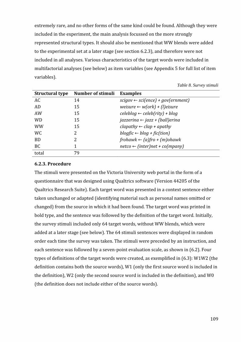
109

extremely rare, and no other forms of the same kind could be found. Although they were

included in the experiment, the main analysis focussed on the more strongly

represented structural types. It should also be mentioned that WW blends were added

to the experimental set at a later stage (see section 6.2.3), and therefore were not

included in all analyses. Various characteristics of the target words were included in

multifactorial analyses (see below) as item variables (see Appendix 5 for full list of item

variables).

Table 8. Survey stimuli

Structural type Number of stimuli Examples

AC 14 scigov ← sci(ence) + gov(ernment)

AD 15 weisure ← w(ork) + (l)eisure

AW 15 celeblog ← celeb(rity) + blog

WD 15 jazzerina ← jazz + (ball)erina

WW 15 clapathy ← clap + apathy

WC 2 blogfic ← blog + fic(tion)

BD 2 frohawk ← (a)fro + (m)ohawk

BC 1 netco ← (inter)net + co(mpany)

total 79

6.2.3. Procedure

The stimuli were presented on the Victoria University web portal in the form of a

questionnaire that was designed using Qualtrics software (Version 44205 of the

Qualtrics Research Suite). Each target word was presented in a context sentence either

taken unchanged or adapted (identifying material such as personal names omitted or

changed) from the source in which it had been found. The target word was printed in

bold type, and the sentence was followed by the definition of the target word. Initially,

the survey stimuli included only 64 target words, without WW blends, which were

added at a later stage (see below). The 64 stimuli sentences were displayed in random

order each time the survey was taken. The stimuli were preceded by an instruction, and

each sentence was followed by a seven-point evaluation scale, as shown in (6.2). Four

types of definitions of the target words were created, as exemplified in (6.3): W1W2 (the

definition contains both the source words), W1 (only the first source word is included in

the definition), W2 (only the second source word is included in the definition), and W0

(the definition does not include either of the source words).

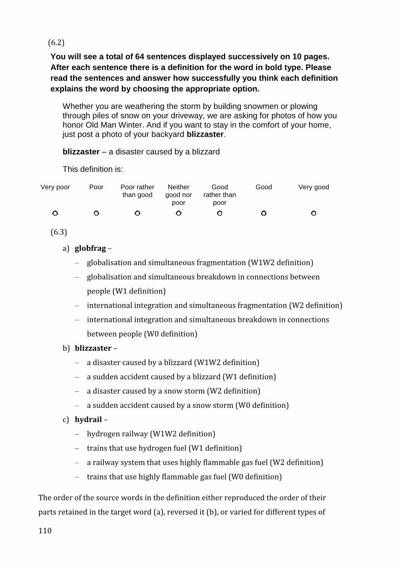
110

(6.2)

You will see a total of 64 sentences displayed successively on 10 pages.

After each sentence there is a definition for the word in bold type. Please

read the sentences and answer how successfully you think each definition

explains the word by choosing the appropriate option.

Whether you are weathering the storm by building snowmen or plowing through piles of snow on your driveway, we are asking for photos of how you honor Old Man Winter. And if you want to stay in the comfort of your home, just post a photo of your backyard blizzaster.

blizzaster – a disaster caused by a blizzard

This definition is: Very poor Poor Poor rather

than good Neither

good nor poor

Good rather than

poor

Good Very good

(6.3)

a) globfrag –

– globalisation and simultaneous fragmentation (W1W2 definition)

– globalisation and simultaneous breakdown in connections between

people (W1 definition)

– international integration and simultaneous fragmentation (W2 definition)

– international integration and simultaneous breakdown in connections

between people (W0 definition)

b) blizzaster –

– a disaster caused by a blizzard (W1W2 definition)

– a sudden accident caused by a blizzard (W1 definition)

– a disaster caused by a snow storm (W2 definition)

– a sudden accident caused by a snow storm (W0 definition)

c) hydrail –

– hydrogen railway (W1W2 definition)

– trains that use hydrogen fuel (W1 definition)

– a railway system that uses highly flammable gas fuel (W2 definition)

– trains that use highly flammable gas fuel (W0 definition)

The order of the source words in the definition either reproduced the order of their

parts retained in the target word (a), reversed it (b), or varied for different types of

111

definitions (c). This was not manipulated purposefully, but was a consequence of

expressing the meaning of a compound-like formation by a phrase. The reason for this is

that syntagmatic origin blends are normally right-headed, as are most English

compounds (Bauer 2009), and the definitions take the left head which is characteristic

of phrases. The order of the source words of paradigmatic origin blends like (a) above,

on the other hand, is not determined by semantics. The general intention was to make

all the definitions sound as natural as possible (given the restrictions imposed by the

definition type), and to explain the target word as successfully as possible, irrespective

of the source word order and the number of source words retained. To achieve this, I

asked 10 native speakers of English to read the full list of sentences with the stimuli and

with all four definitions for each target word and to comment upon how successfully

they thought the definitions explained the meaning of the target words. The feedback

and comments from the testers were taken into consideration, and some definitions

were rephrased. Even these measures could not, however, guarantee that the glosses are

equivalent to the words they replace. There remains a possibility that the judgements

about the quality of definitions might be affected not by the presence of the source

words, but by some other factor influencing the appropriateness of the gloss, which is

not accounted for in this study. Nevertheless, because there is no obvious way of

measuring the appropriateness of the gloss and because the judgements regarding it are

likely to be subjective, it seems appropriate to focus on the influence of the experimental

factor, i.e. the presence of the source words in the definition, and to assume that all other

influences can be treated as random item factors.

Four groups of stimuli were created, so that each target word had a definition from one

of the four types in each group, and so that each group contained equal numbers of

W1W2, W1, W2 and W0 definitions. The participants were randomly assigned to one of

the four groups (27, 28, 28 and 29 participants, out of the 112 whose responses were

included in the analysis). The survey was run with 64 stimuli (only two-element blends

or clipping compounds that included some degree of shortening, i.e. AC, AD, AW, WD,

WC, BD, and BC forms, see Table 1 above). Preliminary results of the study suggested

that that it would be valuable to also assess fully overlapping WW blends because it

appeared that the full preservation of source words was emerging as a significant factor

influencing the evaluation of blend definitions. An additional survey was therefore

created with just the 15 WW target words and their definitions. The methods of

presenting the stimuli and assigning them to the groups according to the definition type

112

were exactly the same as described above. An e-mail was sent to the participants of the

previous survey (99 e-mails were collected for the purpose of the prize draw, the names

of the addressees were not known to the researcher) asking them to answer 15

additional questions. Out of the 99 participants that received the invitations, 58

completed the survey. No responses had to be excluded from the analysis, so all 58 were

included. Because the email addresses in the new survey were not connected to the

demographic data in the old survey (for the sake of anonymity), the demographic

questions were included only in the main survey. Therefore, the information about the

participants’ age group, sex and linguistics education could not be used in the analyses

which included WW blends, but all analyses included participant as a random factor.

6.2.4. Methods of analysis

It is often the case in linguistic studies that the effect of the experimental conditions can

be quite hard to estimate because of the presence of many other effects which are not

part of the experimental design. In this survey, the readers can evaluate the definitions

of target words as more or less appropriate depending on many factors, such as the

length of the blend itself and its source words, their frequency, orthographic or phonetic

similarity, and many other factors which are not experimental variables. A way to

approach this situation is to control for as many factors as possible by including the

known properties of target words as factors in a statistical analysis. So, a number of

characteristics of target words, and also demographic information about the

participants were included in the analyses presented below. In the course of the

analysis, it was sometimes necessary to choose between various ways to define certain

item characteristics. Thus, various measures of similarity of blend words to their source

words were used, including the orthographic similarity measure described in van Orden

(1987). However, a simpler method of calculating the degree of similarity that is

described below turned out to produce the predictor variable which outperformed other

measures of similarity. Similarly, the method of calculating the average similarity

between the source words and the blend by Levenshtein distance (see the discussion of

item variables below) was selected as the most effective from several methods.

The statistical analysis of the survey results involved two qualitatively different

approaches: conditional inference tree and mixed effects multiple regression modelling.

The conditional inference tree (decision tree) method was used at various stages of the

analysis, in order to estimate the hierarchy of independent variables that have

113

significant influence on the dependent variable. This methodology was discussed in

Chapter 4 (see also Hothorn et al. (2006) for more details). The results of the decision

tree analysis were then used to inform the selection of factors in the regression analysis.

The influence of the two experimental variables on the dependent variable (alongside

the influence of other item and participant factors) was estimated in a series of mixed

effects regression models. For regression modelling, the dependent variable was

transformed from a scalar value (having seven possible levels ranging from ‘Very poor’

to ‘Very good’) to a numeric value ranging from 1 to 7 (1 standing for ‘Very poor’, and 7

for ‘Very good’). It has to be noted that presenting the scalar dependent variable in the

form of a numeric one is an approximation, but this approximation provides a means of

building more easily interpretable regression models, with more degrees of freedom

(the latter is especially important when including interactions in the models). The

assumption which underlies the decision to present the scalar variable as a numeric one

is that there is an underlying continuous value (in this case, the ‘goodness’ of definition)

which is indirectly measured on the scale used in the questionnaire. The relationship

between this underlying variable and the independent variables will therefore be

analysed in the regression models (see Bock and Diday (2000) for a discussion of such

an approach to scalar variables).

The role of each factor and of possible interactions of factors was estimated by building

a series of regression models which included different independent variables and by

selecting the models that best predict the observed results. To separate out the effect of

the experimental variables from all the other effects, I used a two-step approach to

regression modelling (Hofmeister 2011). First, all variables except the experimental

ones were used to build a series of regression models, and a model which best explained

the influence of different factors on the response was selected out of the series. At the

second stage a new model was built which used the residuals from the first model as the

dependent variable, and which was used to estimate the influence of the experimental

conditions on it. All statistical analyses were performed using the R software package (R

Development Core Team 2012).

6.3 Results and discussion

The analysis below is based on responses received from 112 participants to the 64 items

of the main survey, and from 58 participants to the 15 items of the additional survey.

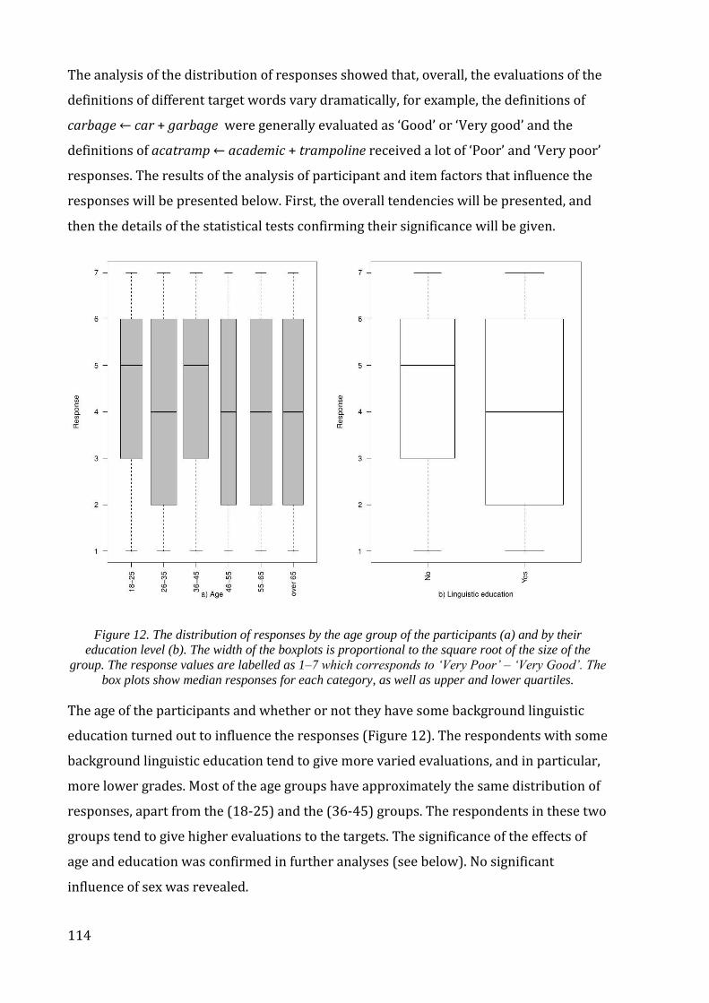
114

The analysis of the distribution of responses showed that, overall, the evaluations of the

definitions of different target words vary dramatically, for example, the definitions of

carbage ← car + garbage were generally evaluated as ‘Good’ or ‘Very good’ and the

definitions of acatramp ← academic + trampoline received a lot of ‘Poor’ and ‘Very poor’

responses. The results of the analysis of participant and item factors that influence the

responses will be presented below. First, the overall tendencies will be presented, and

then the details of the statistical tests confirming their significance will be given.

Figure 12. The distribution of responses by the age group of the participants (a) and by their

education level (b). The width of the boxplots is proportional to the square root of the size of the

group. The response values are labelled as 1–7 which corresponds to ‘Very Poor’ – ‘Very Good’. The

box plots show median responses for each category, as well as upper and lower quartiles.

The age of the participants and whether or not they have some background linguistic

education turned out to influence the responses (Figure 12). The respondents with some

background linguistic education tend to give more varied evaluations, and in particular,

more lower grades. Most of the age groups have approximately the same distribution of

responses, apart from the (18-25) and the (36-45) groups. The respondents in these two

groups tend to give higher evaluations to the targets. The significance of the effects of

age and education was confirmed in further analyses (see below). No significant

influence of sex was revealed.

115

In terms of the structural type of the target words, the median response for the

definitions of AW, WD and WW forms is higher than for the definitions of AC and AD

forms (Figure 13a). In terms of definition type (Figure 13b) the responses tend to be

lower for the definitions containing no source words (W0) than for definitions

containing one of the source words (W1 or W2) or both (W1W2).

Figure 13. The distribution of responses by structural type of the target word (a) and by definition type

(b).

The observed median responses differ across definition types in ways that reflect

differences between the structural types of the target words. For AW, BC, WD and WW

blends the median responses are the same for all four types of definitions, whilst the

definitions of AC, AD, BD and WC target words are given higher evaluations if they

contain the source words (see Table 9).

The results of an ANOVA show that both the effect of blend type and that of definition

type on the response is significant (F[4, 6872]=69.58, p<0.0001 for blend type; F[3,

6872]=6.06, p=0.0004 for definition type). Moreover, the effect of the interaction of

blend type and definition type on the response is also significant (F[12, 6872]=2.35,

p=0.0052). It has to be noted, however, that the observed effect could be due to factors

other than blend type or definition type, or could be a cumulative effect of several

different factors. This is especially important in a situation when, as in the present study,

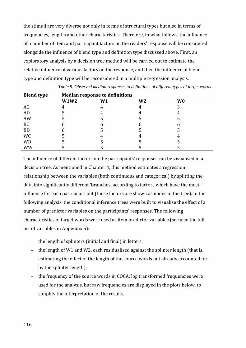
116

the stimuli are very diverse not only in terms of structural types but also in terms of

frequencies, lengths and other characteristics. Therefore, in what follows, the influence

of a number of item and participant factors on the readers’ response will be considered

alongside the influence of blend type and definition type discussed above. First, an

exploratory analysis by a decision tree method will be carried out to estimate the

relative influence of various factors on the response, and then the influence of blend

type and definition type will be reconsidered in a multiple regression analysis.

Table 9. Observed median responses to definitions of different types of target words

Blend type Median response to definitions W1W2 W1 W2 W0

AC 4 4 4 3 AD 5 4 4 4 AW 5 5 5 5 BC 6 6 6 6 BD 6 5 5 5 WC 5 4 4 4 WD 5 5 5 5 WW 5 5 5 5

The influence of different factors on the participants’ responses can be visualised in a

decision tree. As mentioned in Chapter 4, this method estimates a regression

relationship between the variables (both continuous and categorical) by splitting the

data into significantly different ‘branches’ according to factors which have the most

influence for each particular split (these factors are shown as nodes in the tree). In the

following analysis, the conditional inference trees were built to visualise the effect of a

number of predictor variables on the participants’ responses. The following

characteristics of target words were used as item predictor variables (see also the full

list of variables in Appendix 5):

– the length of splinters (initial and final) in letters;

– the length of W1 and W2, each residualised against the splinter length (that is,

estimating the effect of the length of the source words not already accounted for

by the splinter length);

– the frequency of the source words in COCA: log transformed frequencies were

used for the analysis, but raw frequencies are displayed in the plots below, to

simplify the interpretation of the results;

117

– the log transformed frequency of the blend word measured by the number of hits

in Google search (as, for obvious reasons, COCA frequency could not be used for

blends – see the discussion of data collection in section 4.1);

– the semantic type of the target word, that is, whether it is of paradigmatic origin,

e.g. weisure (meaning both work and leisure)or of syntagmatic origin, e.g.

intellidating (meaning ‘intelligent dating’), as discussed in section 4.1;

– the orthographic similarity of the source words to the target words, i.e. the

number of letters that the target word, e.g. advergame shares with the source

word, e.g. advertisement, divided by total number of letters in the source word,

calculated separately for W1 and W2;

– the average string edit distance (ASED) between the source words and the target

word, also known as Levenshtein distance (Levenshtein, 1966), and calculated in

the following way (Gries, 2012): (W1 → Blend + W2 → Blend) /2, i.e. the average

of the number of letters that have to be inserted/deleted/substituted to turn W1

into the target word plus the number of insertions/deletions/substitutions that

are necessary to turn W2 into the target word;

– whether the target word preserves the prosodic pattern (i.e. the number of

syllables and the main stress position) of W1 or W2, or none of them;

– the frequency position of the source words in COCA among all the words

beginning/ending with the letter string in the splinter (that is, whether the

source words are the most frequent among all the words in COCA beginning or

ending with that letter string, see also Appendix 5 for details);

– the COCA frequency of the coordinative combination (with and, or, or a comma)

of the source words of the target word;

– the COCA frequency of the subordinative combination of the source words of the

target word

– the structural type of the target word, i.e. AC, AD, AW, WD, or WW;

– the type of the definition, i.e. W1W2, W1, W2, or W0.

In addition to the item variables, the participants’ age, sex, and background linguistic

education were included in the analysis as participant variables. However, the

participant variables could only be accounted for when analysing the data from the main

survey (that is, the responses to the 64 target words of AC, AD, AW and WD types). The

analysis including the data from the additional survey on 15 WW blends included only

item variables.

118

Not all variables that were initially included in the analysis actually appear in the

decision trees and in the regression models. Firstly, the decision trees do not display

variables which do not have significant influence on the dependent variable. Secondly,

some of the variables considered for including in regression models highly correlated

with each other, which meant that some steps had to be taken in order to de-correlate

them. In the process of regression model building, some predictors were residualised

against one another or entirely excluded for this reason (see Dormann et al. (2013) for

this approach to reducing multicollinearity in the data). Random intercepts for items

and participants, and also random slopes where relevant, were added to the regression

models because they account for item and participant properties not measured directly.

To save space, the responses are presented in the plots below on a scale from 1 to 7,

rather than on a scale from ‘Very poor’ to ‘Very good’. However, it should be kept in

mind that the response in this study is not a continuous measure like, for example,

height or temperature, but, rather, an ordinal variable. This means that each response is

a value on a scale with presumably unknown distances between the neighbouring values

(it is assumed, for instance that ‘Very good’ is a higher value than ‘Good’ and ‘Good’ is a

higher value than ‘Good rather than poor’, but it is not known whether the distance

between the first pair of values is equal to the distance between the second pair). For

these reasons, the type of the decision tree analysis below was ordinal regression, and

therefore the results displayed in Figures 14–16 are not in terms of mean values, but,

rather, in terms of distributions of the responses shown as bar plots in the terminal

nodes of the trees.

In what follows, the analysis of the combined data from the main and the additional

survey will be presented. Therefore, the focus will be on the item factors because the

participant statistics was not collected in the additional survey and therefore could not

be included in the combined data analysis. In addition to the combined data analysis, the

analysis of the main survey only will be presented, to estimate the influence of the

participant factors.

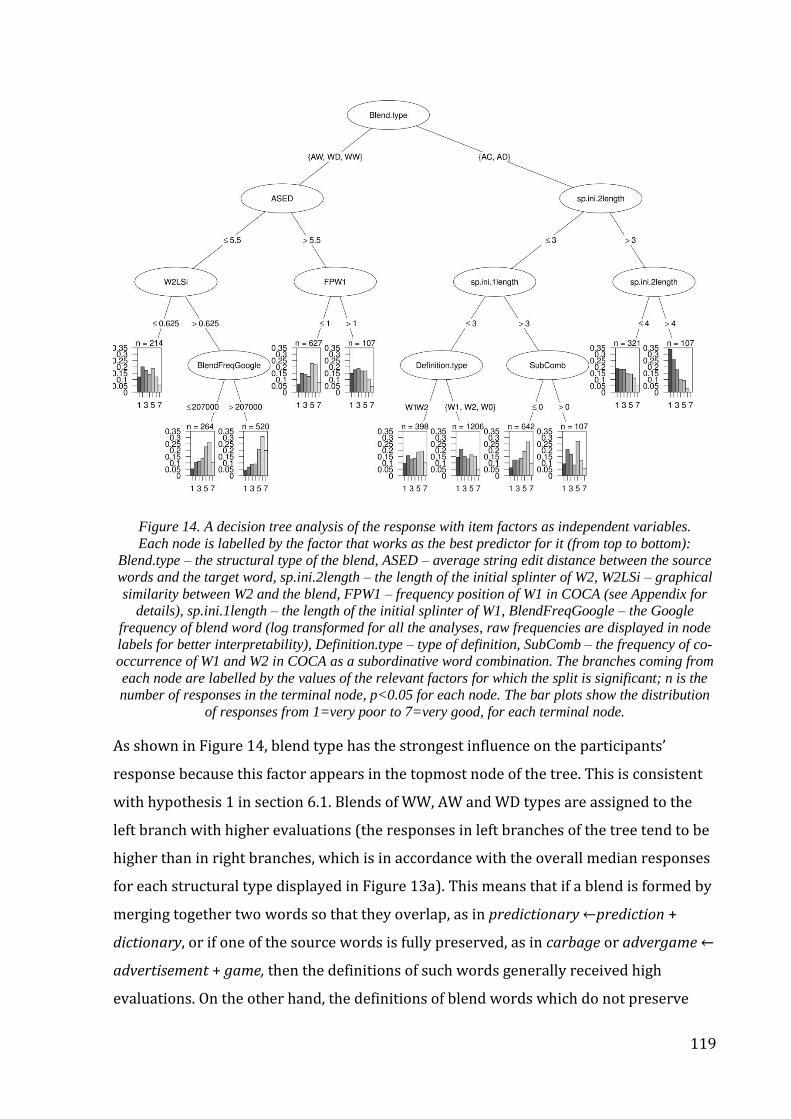
119

Figure 14. A decision tree analysis of the response with item factors as independent variables.

Each node is labelled by the factor that works as the best predictor for it (from top to bottom):

Blend.type – the structural type of the blend, ASED – average string edit distance between the source

words and the target word, sp.ini.2length – the length of the initial splinter of W2, W2LSi – graphical

similarity between W2 and the blend, FPW1 – frequency position of W1 in COCA (see Appendix for

details), sp.ini.1length – the length of the initial splinter of W1, BlendFreqGoogle – the Google

frequency of blend word (log transformed for all the analyses, raw frequencies are displayed in node

labels for better interpretability), Definition.type – type of definition, SubComb – the frequency of co-

occurrence of W1 and W2 in COCA as a subordinative word combination. The branches coming from

each node are labelled by the values of the relevant factors for which the split is significant; n is the

number of responses in the terminal node, p<0.05 for each node. The bar plots show the distribution

of responses from 1=very poor to 7=very good, for each terminal node.

As shown in Figure 14, blend type has the strongest influence on the participants’

response because this factor appears in the topmost node of the tree. This is consistent

with hypothesis 1 in section 6.1. Blends of WW, AW and WD types are assigned to the

left branch with higher evaluations (the responses in left branches of the tree tend to be

higher than in right branches, which is in accordance with the overall median responses

for each structural type displayed in Figure 13a). This means that if a blend is formed by

merging together two words so that they overlap, as in predictionary ←prediction +

dictionary, or if one of the source words is fully preserved, as in carbage or advergame ←

advertisement + game, then the definitions of such words generally received high

evaluations. On the other hand, the definitions of blend words which do not preserve

120

any of their source words in full, such as weisure ← work + leisure, and of clipping

compounds such as scigov, were less frequently evaluated as good or very good.

Therefore, AD and AC forms appear in the right branch of the tree with lower

evaluations.

A number of other predictors appear in the tree which means they also have a

significant effect on the response (the higher the node in the tree the greater predictive

power the corresponding variable has). The numbers displayed on top of terminal nodes

indicate the number of responses in each node. The nodes with small n are informative

as descriptive statistics, rather than as a basis for generalisations. More valuable

information can be drawn from analysing nodes with larger n and tracking down (or up)

the tree in order to see which factors have a significant influence on the responses to

larger groups of target words. For instance, the responses to AW, WD and WW blend

definitions appear to depend on the mean similarity of the two source words to the

blend (ASED) and the frequency position of W1 (FPW1). The definitions of AW, WD and

WW blends which are relatively similar to their source words, i.e. with ASED less than

5.5 (e.g. intellidating ← intelligent + dating), tend to receive higher evaluations than

those of blends which are relatively less similar to both the source words (ASED greater

than or equal 5.5). In the latter group, higher evaluations are received if W1 of the blend

is the most frequent word among all the words beginning with a particular letter string:

this is measured by frequency position (FPW1, e.g. 1 for advergames ← advertisement +

games, and 15 for chofa ← chair + sofa). For ASED=5.5 or less orthographic similarity of

W2 to the target word (W2LSi) is significant: for less similar words (W2LSi=0.625 or

lower), lower evaluations are given.

The evaluations of definitions of AC and AD target words (right branches of the tree)

appear to be sensitive to a different set of factors than those of AW, WD and WW blends.

These factors are the length of the initial splinter of W2 (sp.ini.2length) and W1

(sp.ini.1length), and, for the blends with both initial splinters of 3 letters or less, the type

of definition (Definition.type). For a subset of the data corresponding to 1602 responses

(the sum of 396 and 1206 in the two terminal nodes under the Definition.type node),

W1W2 definitions receive fewer ‘Very poor’ / ‘Poor’ responses and more ‘Good’

responses than the other three types of definitions. The relevant nodes include 9

clipping compounds out of 14, and 7 AD blends out of 15, and all of them preserve fewer

than 3 graphemes of the beginning of the first source word (that is, the length of the

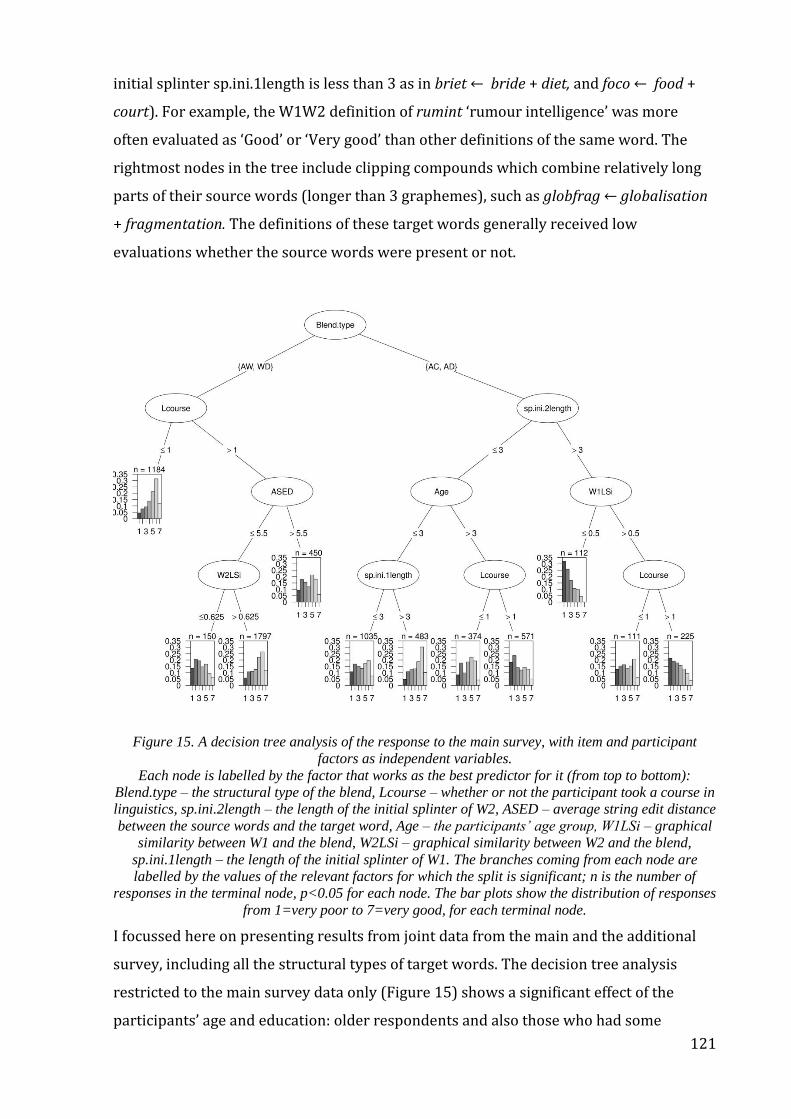
121

initial splinter sp.ini.1length is less than 3 as in briet ← bride + diet, and foco ← food +

court). For example, the W1W2 definition of rumint ‘rumour intelligence’ was more

often evaluated as ‘Good’ or ‘Very good’ than other definitions of the same word. The

rightmost nodes in the tree include clipping compounds which combine relatively long

parts of their source words (longer than 3 graphemes), such as globfrag ← globalisation

+ fragmentation. The definitions of these target words generally received low

evaluations whether the source words were present or not.

Figure 15. A decision tree analysis of the response to the main survey, with item and participant

factors as independent variables.


Blend.type – the structural type of the blend, Lcourse – whether or not the participant took a course in

linguistics, sp.ini.2length – the length of the initial splinter of W2, ASED – average string edit distance

between the source words and the target word, Age – the participants’ age group, W1LSi – graphical

similarity between W1 and the blend, W2LSi – graphical similarity between W2 and the blend,

sp.ini.1length – the length of the initial splinter of W1. The branches coming from each node are

labelled by the values of the relevant factors for which the split is significant; n is the number of

responses in the terminal node, p<0.05 for each node. The bar plots show the distribution of responses

from 1=very poor to 7=very good, for each terminal node.

I focussed here on presenting results from joint data from the main and the additional

survey, including all the structural types of target words. The decision tree analysis

restricted to the main survey data only (Figure 15) shows a significant effect of the

participants’ age and education: older respondents and also those who had some

122

linguistic education tend to give lower evaluations to the definitions, which is

compatible with the distributions displayed in Figure 12 above.

Figure 16. A decision tree analysis of the response to the main survey, with item factors as

independent variables.


Blend.type – the structural type of the blend, ASED – average string edit distance between the source

words and the target word, sp.ini.2length – the length of the initial splinter of W2, W2LSi – graphical

similarity between W2 and the blend, FPW1 – frequency position of W1 in COCA, sp.ini.1length – the

length of the initial splinter of W1, W1LSi – graphical similarity between W1 and the blend,

SemanticType – whether the target word is of syntagmatic (synt) or paradigmatic (para) origin,

Definition.type – type of definition, SubComb – the frequency of co-occurrence of W1 and W2 in

COCA as a subordinative word combination. The branches coming from each node are labelled by the

values of the relevant factors for which the split is significant; n is the number of responses in the

terminal node, p<0.05 for each node. The bar plots show the distribution of responses from 1=very

poor to 7=very good, for each terminal node.

The results of the analysis shown in Figure 15 confirm that blends containing one of the

source words in full (AW and WD) receive higher ratings than blends containing only

clipped forms (AD and AC). The effects of the splinter length and the orthographical

similarity between the source words and the blend are also observed in the main survey

analysis. The definition type, on the other hand, does not appear in the tree, which

means that the effect of the definition type is no longer significant once the effects of

participant variables are accounted for. To check this, another decision tree of the main

123

survey data was built, this time with item predictor variables only. The decision tree in

Figure 16 is very similar to the one in Figure 14, which is not surprising because most of

the data used for the two trees are the same. It should be noted that among the item

variables that turn out to be significant for the main survey data is the semantic type of

the blend, and not frequency, as was the case with the joint data from the main and the

additional survey. Another difference is in the rightmost node of the tree, corresponding

to AC and AD blends with the initial splinter of more than 3 graphemes. The joint data

tree (Figure 14) assigns the difference in the responses to the length of the initial

splinter, while the main survey tree (Figure 16) assigns this difference to the similarity

of W1 to the target word. This may be due to the fact that some significant differences in

responses relevant to particular subsets of data can be explained by different factors, or

could even be due to random properties of particular target words which cannot be

accounted for in this analysis.

In sum, the decision tree analysis of the responses has shown that the structural type of

the target word has a significant influence on how the definitions of the target words are

evaluated. It has also shown that different sets of item factors are significant predictors

of the responses for AW, WD and WW blends on the one hand, and for AD and AC target

words on the other hand, and that the definition type appears to be significant only for a

subset of the data. To better understand the role of the structural type of the target word

and of the definition type as predictors of the response variable, a multiple regression

analysis was performed. It is essential to complete the analysis above with regression

modelling because the latter can account for random item and participant factors.

As mentioned in section 6.2.4, a two-step approach to regression modelling was applied

in order to more carefully investigate the influence of two experimental variables on the

response. First, a series of models was built to predict the response with regard to

significant effects other than those of blend type and definition type. The models were

built with the same independent item and participant variables as the tree models

above, excluding the two experimental variables. As was the case with the variables in

the tree analyses, W1 length and W2 length were residualised against the length of W1

splinters and W2 splinters, respectively, to avoid high correlations between the

variables. Therefore, the variables ‘w1length’ and ‘w2length’ in the models below stand

for the length of W1 and W2 not already accounted for by the length of the splinters.

Random intercepts for items (qID) and participants (uID) were included in the model, as

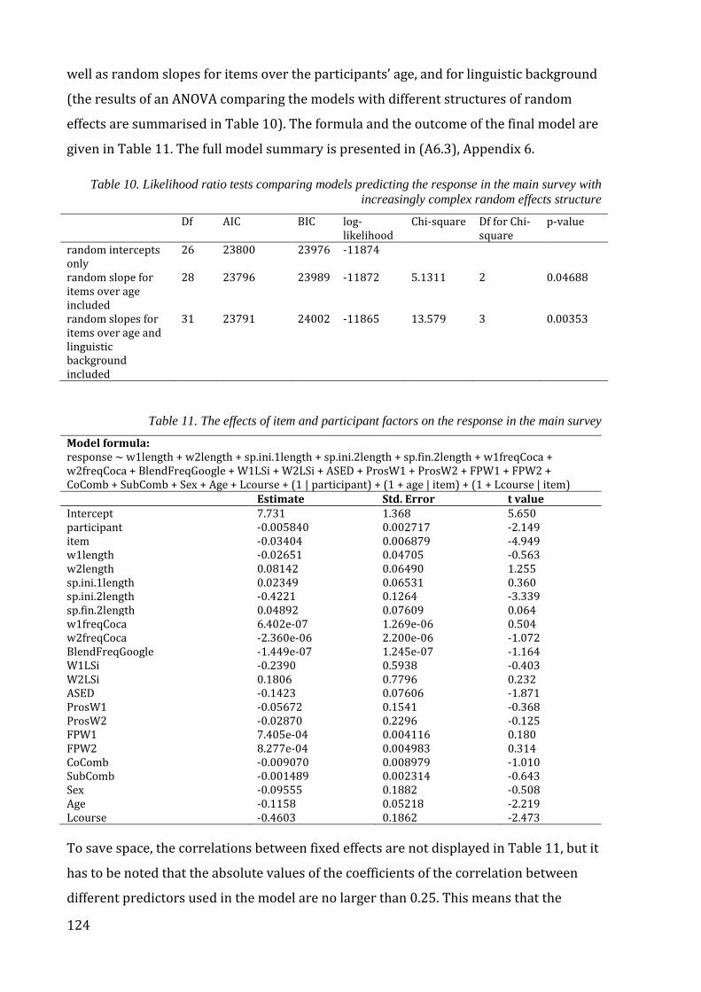
124

well as random slopes for items over the participants’ age, and for linguistic background

(the results of an ANOVA comparing the models with different structures of random

effects are summarised in Table 10). The formula and the outcome of the final model are

given in Table 11. The full model summary is presented in (A6.3), Appendix 6.

Table 10. Likelihood ratio tests comparing models predicting the response in the main survey with

increasingly complex random effects structure

Df AIC BIC log-likelihood

Chi-square Df for Chi-square

p-value

random intercepts only

26 23800 23976 -11874

random slope for items over age included

28 23796 23989 -11872 5.1311 2 0.04688

random slopes for items over age and linguistic background included

31 23791 24002 -11865 13.579 3 0.00353

Table 11. The effects of item and participant factors on the response in the main survey

Model formula: response ~ w1length + w2length + sp.ini.1length + sp.ini.2length + sp.fin.2length + w1freqCoca + w2freqCoca + BlendFreqGoogle + W1LSi + W2LSi + ASED + ProsW1 + ProsW2 + FPW1 + FPW2 + CoComb + SubComb + Sex + Age + Lcourse + (1 | participant) + (1 + age | item) + (1 + Lcourse | item) Estimate Std. Error t value Intercept 7.731 1.368 5.650 participant -0.005840 0.002717 -2.149 item -0.03404 0.006879 -4.949 w1length -0.02651 0.04705 -0.563 w2length 0.08142 0.06490 1.255 sp.ini.1length 0.02349 0.06531 0.360 sp.ini.2length -0.4221 0.1264 -3.339 sp.fin.2length 0.04892 0.07609 0.064 w1freqCoca 6.402e-07 1.269e-06 0.504 w2freqCoca -2.360e-06 2.200e-06 -1.072 BlendFreqGoogle -1.449e-07 1.245e-07 -1.164 W1LSi -0.2390 0.5938 -0.403 W2LSi 0.1806 0.7796 0.232 ASED -0.1423 0.07606 -1.871 ProsW1 -0.05672 0.1541 -0.368 ProsW2 -0.02870 0.2296 -0.125 FPW1 7.405e-04 0.004116 0.180 FPW2 8.277e-04 0.004983 0.314 CoComb -0.009070 0.008979 -1.010 SubComb -0.001489 0.002314 -0.643 Sex -0.09555 0.1882 -0.508 Age -0.1158 0.05218 -2.219 Lcourse -0.4603 0.1862 -2.473

To save space, the correlations between fixed effects are not displayed in Table 11, but it

has to be noted that the absolute values of the coefficients of the correlation between

different predictors used in the model are no larger than 0.25. This means that the

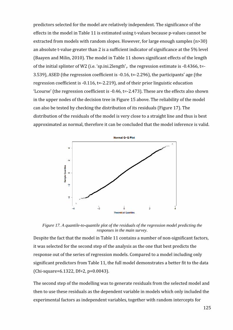
125

predictors selected for the model are relatively independent. The significance of the

effects in the model in Table 11 is estimated using t-values because p-values cannot be

extracted from models with random slopes. However, for large enough samples (n>30)

an absolute t-value greater than 2 is a sufficient indicator of significance at the 5% level

(Baayen and Milin, 2010). The model in Table 11 shows significant effects of the length

of the initial splinter of W2 (i.e. ‘sp.ini.2length’, the regression estimate is -0.4366, t=-

3.539), ASED (the regression coefficient is -0.16, t=-2.296), the participants’ age (the

regression coefficient is -0.116, t=-2.219), and of their prior linguistic education

‘Lcourse’ (the regression coefficient is -0.46, t=-2.473). These are the effects also shown

in the upper nodes of the decision tree in Figure 15 above. The reliability of the model

can also be tested by checking the distribution of its residuals (Figure 17). The

distribution of the residuals of the model is very close to a straight line and thus is best

approximated as normal, therefore it can be concluded that the model inference is valid.

Figure 17. A quantile-to-quantile plot of the residuals of the regression model predicting the

responses in the main survey.

Despite the fact that the model in Table 11 contains a number of non-significant factors,

it was selected for the second step of the analysis as the one that best predicts the

response out of the series of regression models. Compared to a model including only

significant predictors from Table 11, the full model demonstrates a better fit to the data

(Chi-square=6.1322, Df=2, p=0.0043).

The second step of the modelling was to generate residuals from the selected model and

then to use these residuals as the dependent variable in models which only included the

experimental factors as independent variables, together with random intercepts for

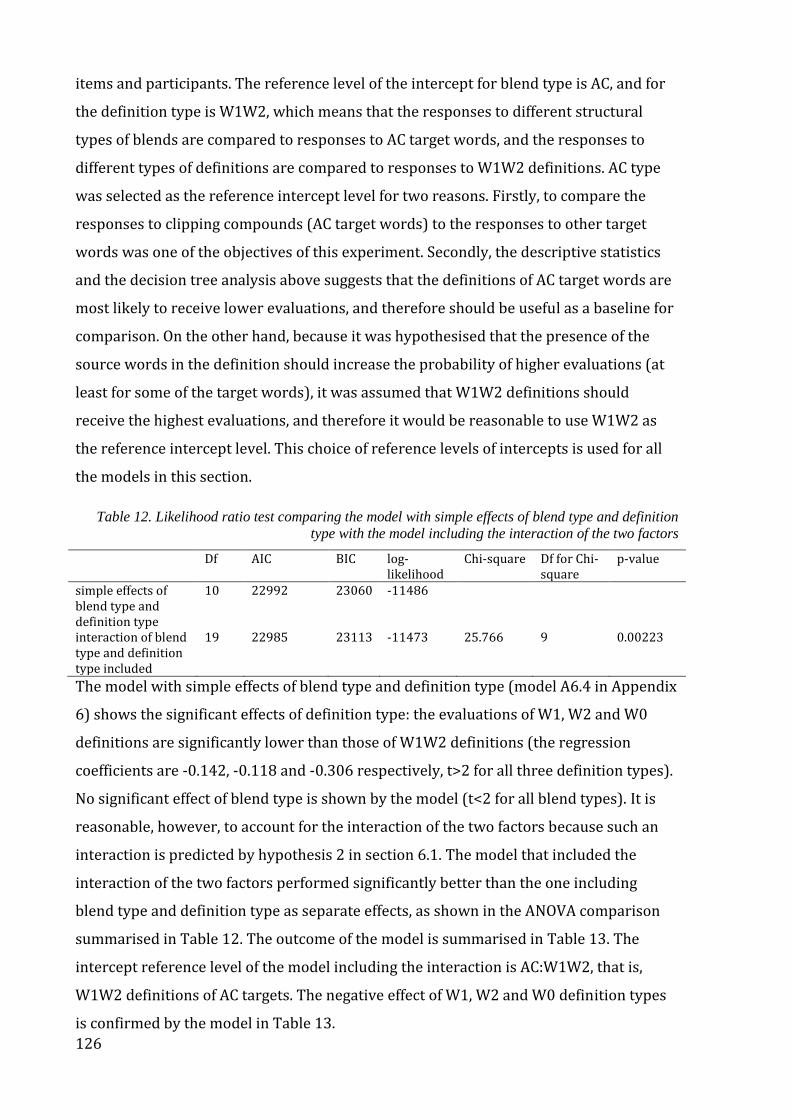
126

items and participants. The reference level of the intercept for blend type is AC, and for

the definition type is W1W2, which means that the responses to different structural

types of blends are compared to responses to AC target words, and the responses to

different types of definitions are compared to responses to W1W2 definitions. AC type

was selected as the reference intercept level for two reasons. Firstly, to compare the

responses to clipping compounds (AC target words) to the responses to other target

words was one of the objectives of this experiment. Secondly, the descriptive statistics

and the decision tree analysis above suggests that the definitions of AC target words are

most likely to receive lower evaluations, and therefore should be useful as a baseline for

comparison. On the other hand, because it was hypothesised that the presence of the

source words in the definition should increase the probability of higher evaluations (at

least for some of the target words), it was assumed that W1W2 definitions should

receive the highest evaluations, and therefore it would be reasonable to use W1W2 as

the reference intercept level. This choice of reference levels of intercepts is used for all

the models in this section.

Table 12. Likelihood ratio test comparing the model with simple effects of blend type and definition

type with the model including the interaction of the two factors



p-value

simple effects of blend type and definition type

10 22992 23060 -11486

interaction of blend type and definition type included

19 22985 23113 -11473 25.766 9 0.00223

The model with simple effects of blend type and definition type (model A6.4 in Appendix

6) shows the significant effects of definition type: the evaluations of W1, W2 and W0

definitions are significantly lower than those of W1W2 definitions (the regression

coefficients are -0.142, -0.118 and -0.306 respectively, t>2 for all three definition types).

No significant effect of blend type is shown by the model (t<2 for all blend types). It is

reasonable, however, to account for the interaction of the two factors because such an

interaction is predicted by hypothesis 2 in section 6.1. The model that included the

interaction of the two factors performed significantly better than the one including

blend type and definition type as separate effects, as shown in the ANOVA comparison

summarised in Table 12. The outcome of the model is summarised in Table 13. The

intercept reference level of the model including the interaction is AC:W1W2, that is,

W1W2 definitions of AC targets. The negative effect of W1, W2 and W0 definition types

is confirmed by the model in Table 13.

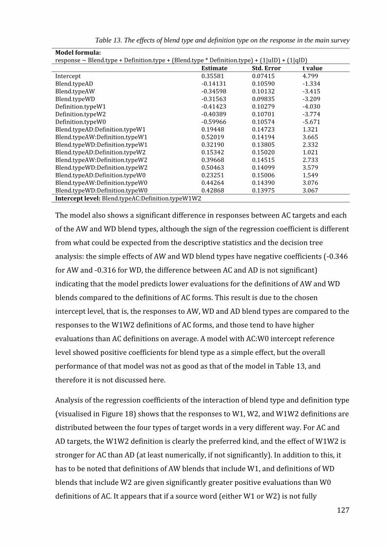
127

Table 13. The effects of blend type and definition type on the response in the main survey

Model formula: response ~ Blend.type + Definition.type + (Blend.type * Definition.type) + (1|uID) + (1|qID) Estimate Std. Error t value Intercept 0.35581 0.07415 4.799 Blend.typeAD -0.14131 0.10590 -1.334 Blend.typeAW -0.34598 0.10132 -3.415 Blend.typeWD -0.31563 0.09835 -3.209 Definition.typeW1 -0.41423 0.10279 -4.030 Definition.typeW2 -0.40389 0.10701 -3.774 Definition.typeW0 -0.59966 0.10574 -5.671 Blend.typeAD:Definition.typeW1 0.19448 0.14723 1.321 Blend.typeAW:Definition.typeW1 0.52019 0.14194 3.665 Blend.typeWD:Definition.typeW1 0.32190 0.13805 2.332 Blend.typeAD:Definition.typeW2 0.15342 0.15020 1.021 Blend.typeAW:Definition.typeW2 0.39668 0.14515 2.733 Blend.typeWD:Definition.typeW2 0.50463 0.14099 3.579 Blend.typeAD:Definition.typeW0 0.23251 0.15006 1.549 Blend.typeAW:Definition.typeW0 0.44264 0.14390 3.076 Blend.typeWD:Definition.typeW0 0.42868 0.13975 3.067 Intercept level: Blend.typeAC:Definition.typeW1W2

The model also shows a significant difference in responses between AC targets and each

of the AW and WD blend types, although the sign of the regression coefficient is different

from what could be expected from the descriptive statistics and the decision tree

analysis: the simple effects of AW and WD blend types have negative coefficients (-0.346

for AW and -0.316 for WD, the difference between AC and AD is not significant)

indicating that the model predicts lower evaluations for the definitions of AW and WD

blends compared to the definitions of AC forms. This result is due to the chosen

intercept level, that is, the responses to AW, WD and AD blend types are compared to the

responses to the W1W2 definitions of AC forms, and those tend to have higher

evaluations than AC definitions on average. A model with AC:W0 intercept reference

level showed positive coefficients for blend type as a simple effect, but the overall

performance of that model was not as good as that of the model in Table 13, and

therefore it is not discussed here.

Analysis of the regression coefficients of the interaction of blend type and definition type

(visualised in Figure 18) shows that the responses to W1, W2, and W1W2 definitions are

distributed between the four types of target words in a very different way. For AC and

AD targets, the W1W2 definition is clearly the preferred kind, and the effect of W1W2 is

stronger for AC than AD (at least numerically, if not significantly). In addition to this, it

has to be noted that definitions of AW blends that include W1, and definitions of WD

blends that include W2 are given significantly greater positive evaluations than W0

definitions of AC. It appears that if a source word (either W1 or W2) is not fully

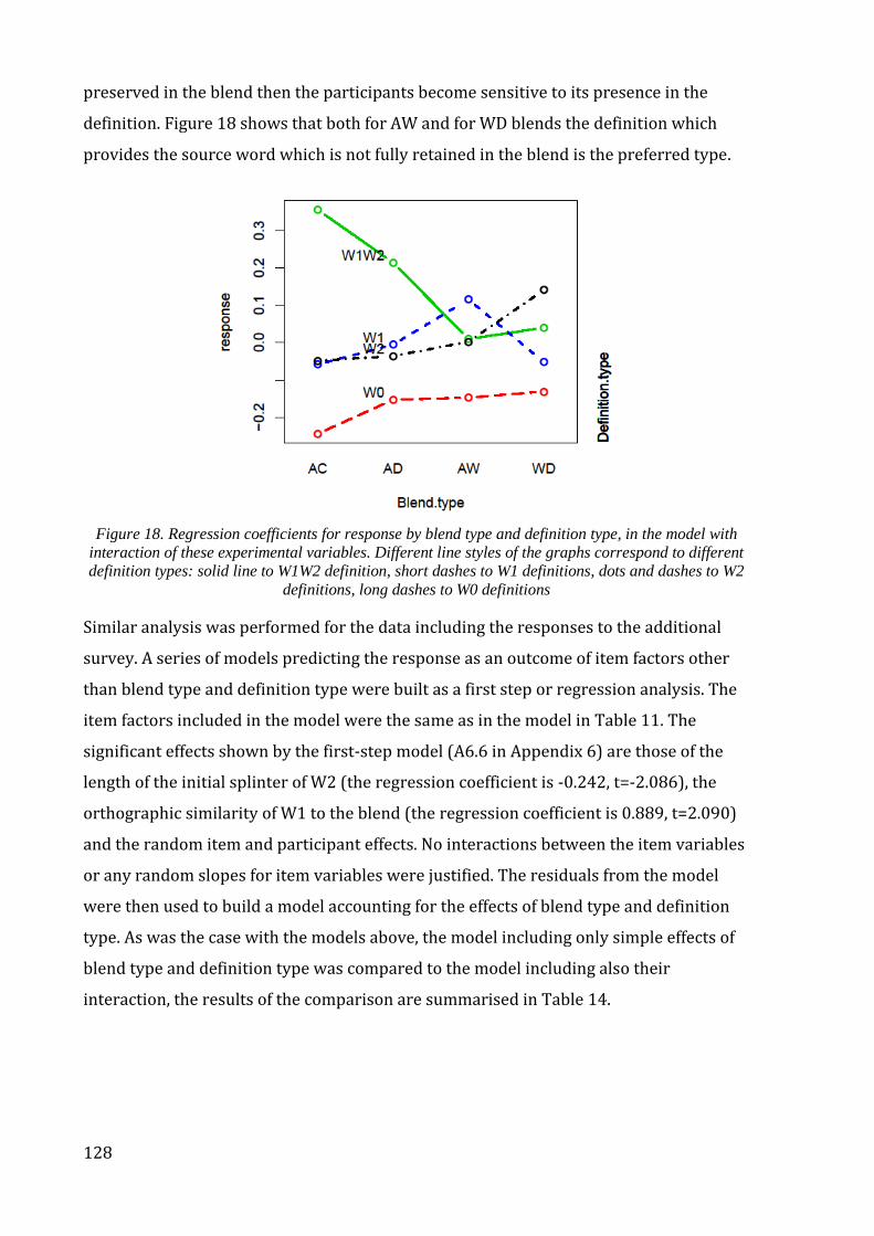
128

preserved in the blend then the participants become sensitive to its presence in the

definition. Figure 18 shows that both for AW and for WD blends the definition which

provides the source word which is not fully retained in the blend is the preferred type.

Figure 18. Regression coefficients for response by blend type and definition type, in the model with

interaction of these experimental variables. Different line styles of the graphs correspond to different

definition types: solid line to W1W2 definition, short dashes to W1 definitions, dots and dashes to W2

definitions, long dashes to W0 definitions

Similar analysis was performed for the data including the responses to the additional

survey. A series of models predicting the response as an outcome of item factors other

than blend type and definition type were built as a first step or regression analysis. The

item factors included in the model were the same as in the model in Table 11. The

significant effects shown by the first-step model (A6.6 in Appendix 6) are those of the

length of the initial splinter of W2 (the regression coefficient is -0.242, t=-2.086), the

orthographic similarity of W1 to the blend (the regression coefficient is 0.889, t=2.090)

and the random item and participant effects. No interactions between the item variables

or any random slopes for item variables were justified. The residuals from the model

were then used to build a model accounting for the effects of blend type and definition

type. As was the case with the models above, the model including only simple effects of

blend type and definition type was compared to the model including also their

interaction, the results of the comparison are summarised in Table 14.

129

Table 14. Likelihood ratio test comparing the model with simple effects of blend type and definition

type with the model including the interaction of the two factors (combined data from the main and the

additional survey)



p-value

simple effects of blend type and definition type

11 25016 25091 -12497

interaction of blend type and definition type included

23 25005 25162 -12480 34.702 12 0.00052

Overall, the output of the regression models in Tables 15 and 16 predicting the

responses to both main and additional survey is very similar to the output of the models

accounting only for the main survey data (which is not surprising because a great part of

the data used for all models is the same).

Table 15. Simple effects of blend type and definition type in the main and the additional survey

Model formula: response ~ Blend.type + Definition.type + (1|uID) + (1|qID) Estimate Std. Error t value Intercept 0.122380 0.050329 2.432 Blend.typeAD -0.010040 0.056266 -0.178 Blend.typeAW -0.007946 0.053582 -0.148 Blend.typeWD -0.011097 0.053577 -0.207 Blend.typeWW 0.017108 0.069088 0.248 Definition.typeW1 -0.124132 0.050319 -2.467 Definition.typeW2 -0.086284 0.050715 -1.701 Definition.typeW0 -0.259037 0.050583 -5.121 Intercept levels: Blend.typeAC, Definition.typeW1W2

Table 16. The effects of blend type and definition type, and the interaction of the two factors in the

main and the additional survey

Model formula: response ~ Blend.type + Definition.type +(Blend.type * Definition.type)+ (1|uID) + (1|qID) Estimate Std. Error t value Intercept 0.36195 0.07886 4.590 Blend.typeAD -0.14014 0.11268 -1.244 Blend.typeAW -0.33244 0.10624 -3.129 Blend.typeWD -0.34681 0.10641 -3.259 Blend.typeWW -0.47334 0.13738 -3.445 Definition.typeW1 -0.42556 0.10953 -3.886 Definition.typeW2 -0.39733 0.11428 -3.477 Definition.typeW0 -0.61075 0.11259 -5.424 Blend.typeAD:Definition.typeW1 0.20014 0.15675 1.277 Blend.typeAW:Definition.typeW1 0.49381 0.14917 3.310 Blend.typeWD:Definition.typeW1 0.36462 0.14933 2.442 Blend.typeWW:Definition.typeW1 0.48853 0.19334 2.527 Blend.typeAD:Definition.typeW2 0.10867 0.16044 0.677 Blend.typeAW:Definition.typeW2 0.37413 0.15270 2.450 Blend.typeWD:Definition.typeW2 0.52732 0.15250 3.458 Blend.typeWW:Definition.typeW2 0.63790 0.19570 3.260 Blend.typeAD:Definition.typeW0 0.22129 0.15992 1.384 Blend.typeAW:Definition.typeW0 0.43791 0.15096 2.901 Blend.typeWD:Definition.typeW0 0.45588 0.15120 3.015 Blend.typeWW:Definition.typeW0 0.84323 0.19528 4.318 Intercept level: Blend.typeAC:Definition.typeW1W2

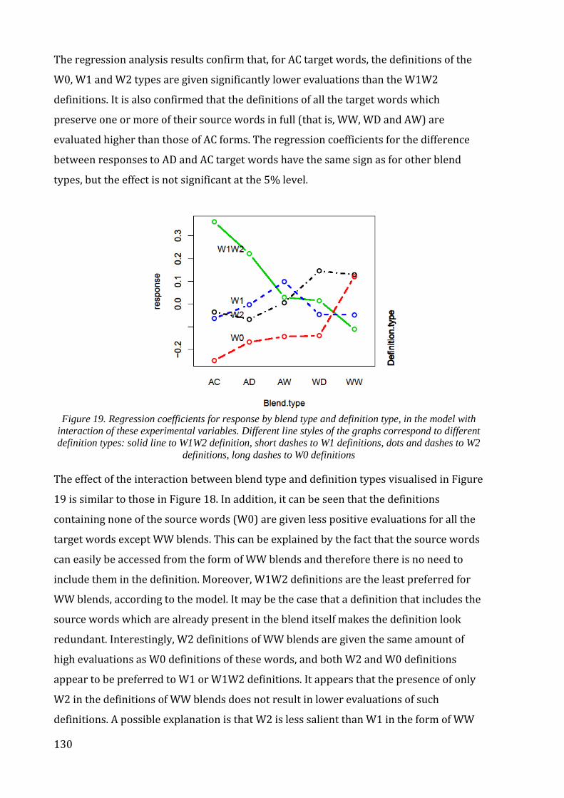
130

The regression analysis results confirm that, for AC target words, the definitions of the

W0, W1 and W2 types are given significantly lower evaluations than the W1W2

definitions. It is also confirmed that the definitions of all the target words which

preserve one or more of their source words in full (that is, WW, WD and AW) are

evaluated higher than those of AC forms. The regression coefficients for the difference

between responses to AD and AC target words have the same sign as for other blend

types, but the effect is not significant at the 5% level.

Figure 19. Regression coefficients for response by blend type and definition type, in the model with

interaction of these experimental variables. Different line styles of the graphs correspond to different

definition types: solid line to W1W2 definition, short dashes to W1 definitions, dots and dashes to W2

definitions, long dashes to W0 definitions

The effect of the interaction between blend type and definition types visualised in Figure

19 is similar to those in Figure 18. In addition, it can be seen that the definitions

containing none of the source words (W0) are given less positive evaluations for all the

target words except WW blends. This can be explained by the fact that the source words

can easily be accessed from the form of WW blends and therefore there is no need to

include them in the definition. Moreover, W1W2 definitions are the least preferred for

WW blends, according to the model. It may be the case that a definition that includes the

source words which are already present in the blend itself makes the definition look

redundant. Interestingly, W2 definitions of WW blends are given the same amount of

high evaluations as W0 definitions of these words, and both W2 and W0 definitions

appear to be preferred to W1 or W1W2 definitions. It appears that the presence of only

W2 in the definitions of WW blends does not result in lower evaluations of such

definitions. A possible explanation is that W2 is less salient than W1 in the form of WW

131

blends because the beginning of W2 does not coincide with the beginning of the blend,

and therefore may not be easily recognised as a word onset (in fact, some of the findings

in Chapter 7 suggest this is the case). The fact that including the interaction between

blend type and definition type has significantly improved the model fit implies that

whether or not the evaluation of the target words’ definition is sensitive to the presence

or absence of their source words, depends on the type of the target words. The decision

tree analysis described above demonstrates qualitative characteristics of the target

words which are more successfully explained by definitions containing both the source

words – these are clipping compounds preserving relatively small portion of the

graphical material of their source words. The outcome of the regression analysis

provides a quantitative estimate of these effects.

6.4. Interim conclusions: Perception and understanding of blends and

clipping compounds

The survey results strongly support the hypothesis that the structural type of the

blend/clipping compound influences the readers’ evaluation of its definition (hypothesis

1). The results also suggest that, when evaluating the definitions of target words, the

readers appear to be sensitive to their structural type. It was confirmed that the readers

give higher evaluations to less formally transparent target words if their source words are

included in the definitions (hypothesis 2). It would be intuitively clear that any blend

word or clipping compound is easier to explain by using the words it is made of, rather

than by paraphrasing them. What is striking about the results of this survey is that this

factor turns out to have an impact on the definitions of a subset of words with specific

characteristics. If the source words cannot be easily recovered from the form of a blend or

a clipping compound (as it appears to be the case for weisure and scigov), then it is

essential to use these words in order to explain the meaning of the blend or clipping

compound. This is also true for cases when only one source word cannot be recovered

from the blend, as the readers give numerically higher evaluations to W1 definitions of

AW blends and W2 definitions of WD blends. That is, the readers seem to prefer

definitions in which the full counterparts of the incomplete splinters of blends are

provided, as in the W1 definition of approximeeting which includes the word approximate,

and in the W2 definition of complimentsult which includes the word insult. On the other

hand, if the source words are recoverable well enough from the blend itself, as in the case

of predictionary, their presence in the definition becomes less important because the

132

formal transparency of the blend enhances the recoverability of their source words. The

results of the survey reveal that the structural type of target words explains the variance

in the response to a considerable extent. The construct of the structural type introduced

in Chapter 4 reflects two aspects of blend formation: formal transparency (that is, full

versus partial preservation of the source words and preserving word beginnings versus

word ends) and, albeit indirectly, recognisability of the source words. The results above

confirm that full preservation of the source words (which is true for AW, WD and WW

blends) makes the respondents less sensitive to the types of definition, which clearly

distinguishes AW, WD and WW target words from the ones which do not preserve the

source words in full (i.e. AD or AC). Having said this, I must admit that different patterns

are observed for AW, WD and WW blends with respect to W1 and W2 definitions. This

means that full preservation of only one of the source words influences the evaluation of

the definitions depending on the presence of that source word in them.

The participants of the survey were asked to evaluate how well each definition explained

the highlighted words. This instruction could potentially be interpreted in two different

ways. On the one hand, the participants could have interpreted it as an invitation to judge

how well the given definitions matched their own interpretations of the stimuli words. On

the other hand, they could be evaluating how well the information provided in the

definitions compensated for their lack of knowledge of the meaning of the stimuli words.

It could also be the case that the choice between the two interpretations varied across

participants, or across items. Although the procedure of this survey did not have a

separate measure of whether or not the participants were able to derive their own ‘a

priori’ interpretation, the observed results suggest that, at least for less transparent types,

the participants appeared to lack the sufficient prior knowledge, and therefore had to rely

upon the definition. This can explain higher evaluations of W1W2 definitions of AD and

AC formations. The present results support the claim in Gries (2006) that recognisability

of the source words can be used as a criterion of well-formedness of blends, which helps

to distinguish them from clipping compounds. The most apparent difference between

evaluations of blends that was revealed in this study is that blends with high degree of

formal transparency, i.e. blends which preserve at least one of their source words in full,

are evaluated differently from those with low formal transparency (AD blends like

blizzaster). Clipping compounds (or AC forms, such as rumint ← rumour + intelligence),

behave similarly to low transparency AD blends. It is worth noting that clipping

compounds seem to be more sensitive to the presence of the source words in the

133

definition than even low transparency blends. Although this tendency did not reach the

level of statistical significance to be revealed in the decision tree or regression analysis,

the overall distribution of the responses by blend type (Figure 13) suggests that clipping

compounds are given lower evaluations than any other target words in the sample. These

observations indicate that clipping compounds may be processed differently from all

types of blends, including lower transparency AD forms. Judging by the low marks words

like rumint get, people have difficulty understanding them, and the only thing that seems

to be able to save the situation is the presence of both their source words in the definition.

However, further study is needed to investigate whether AC forms are significantly

different from AD forms in this respect.

This research is, to the best of my knowledge, the first study of English blends which 1)

attempts to evaluate readers’ understanding of blends by analysing experimentally

induced responses, 2) compares the participants’ evaluation of blends and clipping

compounds. Moreover, the study focusses entirely on novel blends, which distinguishes it

from a number of earlier works in the field. On the one hand, this combination of new

materials and new methods can help look at blending from a new angle and, perhaps, find

‘a flash of insight’ Bauer (2012) hoped for. On the other hand, it means choosing a path

‘less traveled by’, with a lot of bumps on the way, and possibly a dead end. Among the

factors which may be regarded as ‘bumps’ in that they may have caused difficulty in

interpreting the results is, for example, the form of the experiment that was used, that is, a

questionnaire. Such a method implies using a subjective measure of the plausibility of the

definition, which can depend on a variety of factors, both linguistic and extralinguistic,

and only a small number of those (in this case, a few demographic characteristics of the

participants and formal and semantic characteristics of target words) can be formalised

for statistical analysis. When questionnaire responses form the dependent variable for

analysis, a great deal may depend on how the questions were interpreted by the

participants, and whether they were interpreted in the same way as the researcher

expected them to be. In this study there is no guarantee that the responses that were

produced were indeed the evaluations of the definitions, rather than of the target words

themselves. A further study involving online measures and reducing the possibility of

strategic and/or conscious answers on the part of the participants is needed to further

investigate the relationships between the source words’ recognisability and

recoverability, on the one hand, and the processing of the blends and clipping compounds,

on the other hand. Another factor which may have decreased the interpretability of the

134

results is the high degree of variance of the lexical material (various structural types of

the target words, differences in their semantics, length, frequency of the source words,

etc.). It is hardly possible to find a satisfying number of blends and clipping compounds

which would be matched for length, frequency, etc. The results of this research, however,

can help select those characteristics of target words which are important to control

because they appear to influence the participants’ responses to them. For instance, as the

structural type appeared to be an important predictor of the response, I propose

restricting future study to fewer structural types in order to be able to make reliable

comparisons between them. It may be the case that some information will be not

available if we are not testing the full range of structural types which can be found, but

concentrating on fewer distinctly different types of target words can help provide more

well-supported explanations of their processing which can afterwards be tested on more

structural types.

Despite the drawbacks outlined above, the results of this survey provide some clues about

the importance of the different formal properties of the target words, as well as their

understanding. The observed results can be regarded as further evidence, in addition to

those reported, e.g. in Gries (2012) and in Chapter 4 of the present thesis, that the

process of blending results in formations consisting of the beginning of one word and the

ending of another (with a possible overlap), which are different from clipping compounds

(combining the beginnings of two or more words) not only in terms of form, but also in

terms of the relationships between the formation and its source words. The results of the

survey also imply that the relationship between the structure of the blend and its

plausibility from the reader’s point of view is not straightforward, and it is possible that

different cognitive factors are involved in the perception and understanding of blends of

different structural types and of clipping compounds. To get a closer look at the

perception of blends and clipping compounds, I carried out a psycholinguistic experiment

which is discussed in the following chapter. On the one hand, the methods used for the

next stage of this research allow us to look at the recognition of the source words in a

more straightforward way than the questionnaire discussed in this chapter, on the other

hand, I will henceforward use fewer structural types of target words which, as the above

analysis suggests, is more practical for the aims of the study.

135

Chapter 7. Can you find an academic in an acatramp? Priming effect of

blends and clipping compounds on the processing of their source

words

The study described in this chapter has been inspired not only by the analysis of gaps in

the literature on blends and the corpus data analysis, but to a great extent by the results

of the web survey discussed in the previous chapter. In particular, it was found that full

preservation of the source words in a blend word clearly influences the evaluation of the

definition of the blend. It is not so clear, however, whether blend words which do not

preserve any of their source words in full (AD) are significantly different from clipping

compounds (AC) in terms of the recognition of their source words. Both earlier research

and my own analysis of the structural properties of both types of formations suggest

there should be differences. Therefore, the next stage of this research is an experimental

study in which AC and AD forms are compared in terms of the recognition and

processing of the W1 and W2 source words contained in those forms. Both groups will

be compared to WW blends which fully preserve their source words and are therefore

more transparent than both AD and AC.

Studies of visual word recognition reveal different effects of word properties on lexical

decision latencies, as discussed in Chapter 5. The research presented in the current

chapter studies the link between formal transparency (i.e. what portion of the original

word is preserved in the shortening) and the recoverability of meaning in two types of

complex formations: blends and clipping compounds. The results presented in Chapter 6

suggest that WW blends with a higher degree of formal transparency (such as

predictionary) may produce stronger priming of their source words in a lexical decision

task than either AD blends with a lower degree of formal transparency (e.g. scoratorium)

or clipping compounds (e.g. finlit). The experiment involves an unconventional way of

presenting primes via an identification and production task which precedes lexical

decision task.

7.1. Background and rationale

Are blend words processed in the same way as regular and productive formations such

as compounds and derivatives? This question has been approached in a number of

experiments by Lehrer (1996, 2003) and Lehrer and Veres (2010). The researchers tried

to find evidence for rapid and automatic decomposition of blends into their source

136

words, and, as stated in Chapter 5, did not succeed. Nevertheless, the results of Lehrer’s

experiments demonstrated evidence of associations between blends and their source

words in language users’ memories. In particular, presenting a blend in a task which

requires participants to identify its source words results (if the words are recognisable

from the blend) in activation of their mental representations. This in turn can influence

the participants’ performance in a subsequent task (in Lehrer and Veres (2010), a stem

completion task). If this is the case, then different results should be obtained for

different structural types of blends, depending on the recognisability of their source

words. In Lehrer and Veres’ study, blends of four structural types were used as stimuli

for the identification and production task: splinter + word (AW in my notation, e.g.

qualatex ← quality + latex), word + splinter (WD, e.g. beermare ← beer + nightmare), two

splinters (AD, e.g. snizzle ← snow + drizzle) and complete overlap (WW, e.g. palimony ←

pal + alimony). The difference between the structural types found in the study was,

however, not statistically significant (see section 5.2 for details).

For this research I adapted some of the methods used by Lehrer and Veres and used

them on a different set of data to study the differences between processing fully

overlapping WW blends, non-overlapping AD blends (the ‘two splinters’ type in Lehrer’s

terminology) and clipping compounds, or AC forms. Comparing blends with clipping

compounds did not form part of Lehrer and Veres’ study, so this research is not simply a

replication of their experiment. Rather, taking inspiration from their findings, I am

trying to build on them and to extend their implications in new directions. Another

important difference between my experiments and those of Lehrer and Veres is that I

restrict my stimuli to relatively new blends with splinters which are not likely to have

developed into productive combining forms (see criteria in section 4.1). Such a

restriction on data sampling is essential because it allows us to separate the effects of

recognisability of source words from those of lexicalisation (the case of older blends)

and of analogy (the case of productive splinters). Choosing the stimuli for the

experiment, I avoided including blends whose splinters showed signs of productivity,

such as the initial splinter edu- which is a part of edutainment, edupunk, etc., or the final

splinter –noia (present in juvenoia, parentnoia, etc.).

The experiment was designed to verify two hypotheses. The first of them concerns the

actual recognition of the source words of blends and clipping compounds:

137

1) The source words of blends with a higher degree of formal transparency (WW,

e.g. predictionary) will be more easily identified than those of blends with a lower

degree of formal transparency (AD, e.g. blizzaster), and of clipping compounds

(AC, e.g. finlit). It is also hypothesised that because AC forms are less transparent

than any blends (including AD), according to the criteria developed in Chapter 4,

their source words will be less easily identified than the source words of AD

blends.

The second hypothesis concerns the effect of blends or clipping compounds on the

processing of their source words. In a masked priming experiment reported by Lehrer

(2003, 2007), no priming effect of blends on the processing of source words was found

and this result was reported as showing no effect of rapid automatic decomposition of

blend words into their constituents. Assuming that, indeed, blends “present a processing

challenge” (Lehrer, 2003, p. 379), I focussed not on automatic decomposition but on the

effect of prior retrieval of the representation of the source words. Thus, it was decided

not to use blends or clipping compounds as masked or unmasked primes in the lexical

decision task. Rather, the long-term priming effect of the source words retrieved in an

identification and production task was considered to be an experimental variable (see

details of the procedure in section 7.4).

2) Prior exposure to blends will facilitate recognition of their source words in a

lexical decision task. This effect will be greater for blends with a higher degree of

formal transparency (WW) than for blends with a lower degree of formal

transparency (AD). This is because the source words of higher transparency

blends are more likely to be recognised in the identification / production task

which will mediate recognition in the subsequent task. For clipping compounds

(AC) no priming effect is expected.

The conditions for the long-time priming effect were created by combining an

identification and production task and a lexical decision task so that the blends and

clipping compounds used in the former could prime their source words presented as

stimuli in the latter.

7.2. Participants

Native speakers of English were offered gift vouchers for their voluntary participation in

this experiment (the information sheet offered to the participants is provided in

138

Appendix 7, and an example of the consent form filled out by each participant is given in

Appendix 8). Overall, there were 107 participants (37 male and 70 female), recruited

among undergraduate students or staff at Victoria University of Wellington. The age of

participants ranged between 18 and 45, the mean age being 22 years, SD=5.5 years.

7.3. Stimuli

As pointed out above, the objective of the experiment was to compare blends with a high

degree of formal transparency to lower transparency blends and to clipping compounds.

Therefore, three groups of complex formations with different degrees of formal

transparency were contrasted:

- AC forms (clipping compounds), e.g. hydrail ← hydr(ogen) + rail(way) (low

transparency);

- AD blends, e.g. virtopsy ← virt(ual)+ ( au)topsy (moderate transparency);

- WW blends (fully overlapping blends), e.g. stoption ← stop + option (high

transparency)

The notation for the structural types of stimuli was used according to the same criteria

as in Chapter 6, i.e. only those of AC and AD forms which do not preserve either of their

source words in full were selected as experimental stimuli because full versus partial

preservation can be an important factor influencing word recognition and therefore it is

essential to control for it.

In total, 30 words were used for the identification and production task, 10 of each

structural type. All the stimuli were selected from the collection discussed in Chapter 4

and therefore attested in media/ corpora no earlier than 1/1/2000. None of these words

contain productive combining forms registered in dictionaries. However, 6 of 10

clipping compounds contain splinters which appear in other blends or clipping

compounds found either in COCA or among those collected for the present research.

The source words of the blends and clipping compounds were then presented as targets

in a lexical decision task, 60 target words in total. The same number of pseudowords

was also included in the lexical decision task. The pseudowords were created

specifically for this experiment, and were matched with the target words in length and

also in the degree of orthographic similarity to primes. For example, the blend blizzaster

is made of the source words blizzard and disaster so that the letter string blizza- is

139

common for the first source word and the blend, and the letter string -aster for the

second source word and the blend. The corresponding pseudowords blizzant and

colaster have the same letter strings common with the blend blizzaster, and are also

matched with the real words blizzard and disaster for the number of syllables. These

principles were followed with most of the pseudowords orthographically similar to the

real source words of blends and clipping compounds used as stimuli in this experiment.

However, the pseudowords similar to the source words of WW blends demanded a

slightly different approach. As both the source words are fully preserved in blends like

stoption and predictionary, it is impossible to simply retain the relevant part of blend in a

pseudoword because it would repeat an existing word, e.g. stop or dictionary. Therefore,

pseudowords similar to the source words of WW blends were generated from the

corresponding words by replacing some of the letters and/or changing the order of

letters in them, e.g. tosp was generated from stop, and doctoilary was generated from

dictionary. Thus, such pseudowords had the necessary high degree of orthographic

similarity to the source words of blends and at the same time did not look exactly like

real words. The parts of the pseudowords which did not repeat the letter strings from

real words were either taken from ARC online nonword database (Rastle et al. 2002), or

created in such a way that the letter strings resembled those in the database. This

approach to generating pseudowords was maintained to make sure that they followed

general orthographic and phonological restrictions of English. In addition, the list of

experimental stimuli was checked by three native speakers of English, to ensure that

they conformed to the phonological and orthographic constraints of English.

7.4. Procedure

The experiment consisted of two tasks, completed one after another. Both tasks were

created and run in the E-Prime 2.0 software package (Schneider et al. 2002). A response

box with NO, OK, and YES buttons was used to input answers for the two tasks. The

participants were told that they were going to do two tasks, and that they should use the

OK button only for the first task, and YES and NO buttons for the second task.

7.4.1. Task 1: An identification and production task

The stimuli were arranged into two lists, with 15 words in each (5 AD blends, 5 WW

blends, and 5 clipping compounds per list), in order to create a priming condition for the

lexical decision task (see section 7.4.2 for details). The participants were randomly

assigned to two groups (Group 1 and Group 2), so that one Group 1 was shown one list

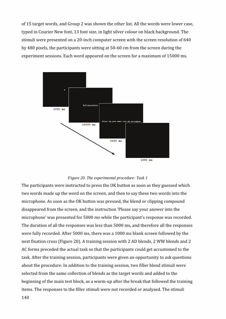
140

of 15 target words, and Group 2 was shown the other list. All the words were lower case,

typed in Courier New font, 13 font size, in light silver colour on black background. The

stimuli were presented on a 20-inch computer screen with the screen resolution of 640

by 480 pixels, the participants were sitting at 50-60 cm from the screen during the

experiment sessions. Each word appeared on the screen for a maximum of 15000 ms.

Figure 20. The experimental procedure: Task 1

The participants were instructed to press the OK button as soon as they guessed which

two words made up the word on the screen, and then to say these two words into the

microphone. As soon as the OK button was pressed, the blend or clipping compound

disappeared from the screen, and the instruction ‘Please say your answer into the

microphone’ was presented for 5000 ms while the participant’s response was recorded.

The duration of all the responses was less than 5000 ms, and therefore all the responses

were fully recorded. After 5000 ms, there was a 1000 ms blank screen followed by the

next fixation cross (Figure 20). A training session with 2 AD blends, 2 WW blends and 2

AC forms preceded the actual task so that the participants could get accustomed to the

task. After the training session, participants were given an opportunity to ask questions

about the procedure. In addition to the training session, two filler blend stimuli were

selected from the same collection of blends as the target words and added to the

beginning of the main test block, as a warm-up after the break that followed the training

items. The responses to the filler stimuli were not recorded or analysed. The stimuli

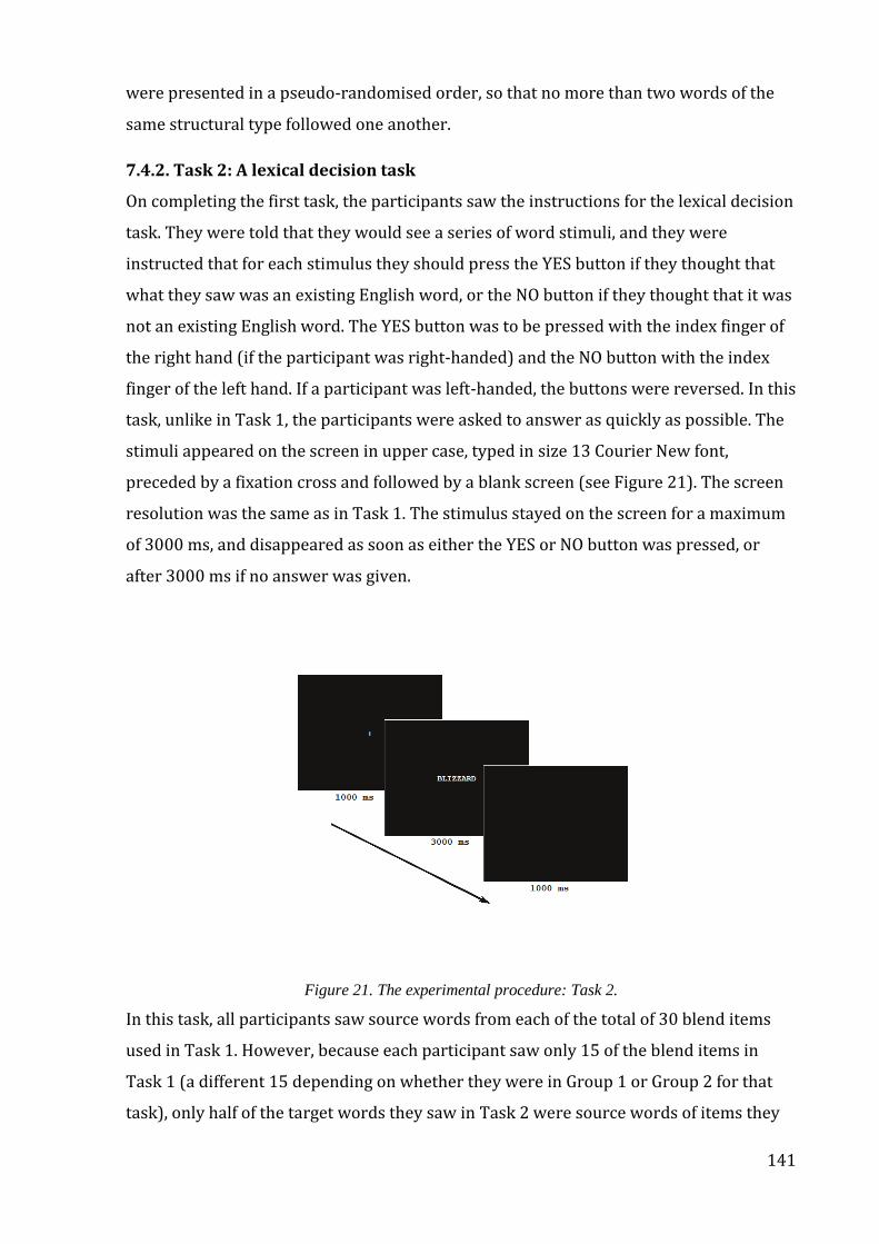
141

were presented in a pseudo-randomised order, so that no more than two words of the

same structural type followed one another.

7.4.2. Task 2: A lexical decision task

On completing the first task, the participants saw the instructions for the lexical decision

task. They were told that they would see a series of word stimuli, and they were

instructed that for each stimulus they should press the YES button if they thought that

what they saw was an existing English word, or the NO button if they thought that it was

not an existing English word. The YES button was to be pressed with the index finger of

the right hand (if the participant was right-handed) and the NO button with the index

finger of the left hand. If a participant was left-handed, the buttons were reversed. In this

task, unlike in Task 1, the participants were asked to answer as quickly as possible. The

stimuli appeared on the screen in upper case, typed in size 13 Courier New font,

preceded by a fixation cross and followed by a blank screen (see Figure 21). The screen

resolution was the same as in Task 1. The stimulus stayed on the screen for a maximum

of 3000 ms, and disappeared as soon as either the YES or NO button was pressed, or

after 3000 ms if no answer was given.

Figure 21. The experimental procedure: Task 2.

In this task, all participants saw source words from each of the total of 30 blend items

used in Task 1. However, because each participant saw only 15 of the blend items in

Task 1 (a different 15 depending on whether they were in Group 1 or Group 2 for that

task), only half of the target words they saw in Task 2 were source words of items they

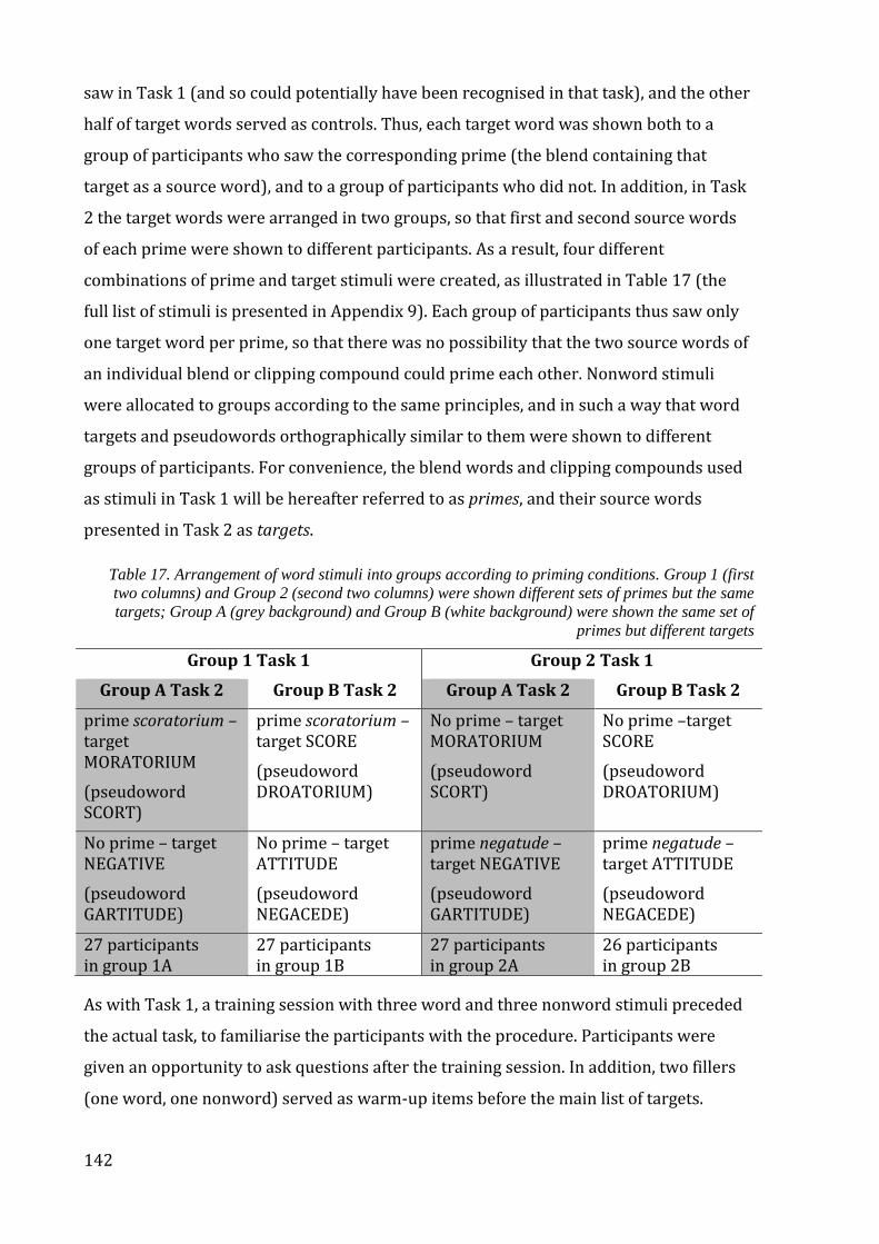
142

saw in Task 1 (and so could potentially have been recognised in that task), and the other

half of target words served as controls. Thus, each target word was shown both to a

group of participants who saw the corresponding prime (the blend containing that

target as a source word), and to a group of participants who did not. In addition, in Task

2 the target words were arranged in two groups, so that first and second source words

of each prime were shown to different participants. As a result, four different

combinations of prime and target stimuli were created, as illustrated in Table 17 (the

full list of stimuli is presented in Appendix 9). Each group of participants thus saw only

one target word per prime, so that there was no possibility that the two source words of

an individual blend or clipping compound could prime each other. Nonword stimuli

were allocated to groups according to the same principles, and in such a way that word

targets and pseudowords orthographically similar to them were shown to different

groups of participants. For convenience, the blend words and clipping compounds used

as stimuli in Task 1 will be hereafter referred to as primes, and their source words

presented in Task 2 as targets.

Table 17. Arrangement of word stimuli into groups according to priming conditions. Group 1 (first

two columns) and Group 2 (second two columns) were shown different sets of primes but the same

targets; Group A (grey background) and Group B (white background) were shown the same set of

primes but different targets

Group 1 Task 1 Group 2 Task 1

Group A Task 2 Group B Task 2 Group A Task 2 Group B Task 2

prime scoratorium – target MORATORIUM

(pseudoword SCORT)

prime scoratorium – target SCORE

(pseudoword DROATORIUM)

No prime – target MORATORIUM

(pseudoword SCORT)

No prime –target SCORE

(pseudoword DROATORIUM)

No prime – target NEGATIVE

(pseudoword GARTITUDE)

No prime – target ATTITUDE

(pseudoword NEGACEDE)

prime negatude – target NEGATIVE

(pseudoword GARTITUDE)

prime negatude – target ATTITUDE

(pseudoword NEGACEDE)

27 participants in group 1A

27 participants in group 1B

27 participants in group 2A

26 participants in group 2B

As with Task 1, a training session with three word and three nonword stimuli preceded

the actual task, to familiarise the participants with the procedure. Participants were

given an opportunity to ask questions after the training session. In addition, two fillers

(one word, one nonword) served as warm-up items before the main list of targets.

143

In sum, the following targets were presented to each of the four groups (1A, 1B, 2A and

2B), arranged in such a way that formal overlap between items seen in a) to h) was

minimised:

(7.1)

a) first source words of blends/clipping compounds that were previously shown in

Task 1

b) first source words of blends/clipping compounds that were not shown in Task 1

c) second source words of blends/clipping compounds that were previously shown

in Task 1

d) second source words of blends/clipping compounds that were not shown in Task 1

e) pseudowords orthographically similar to (a)

f) pseudowords orthographically similar to (b)

g) pseudowords orthographically similar to (c)

h) pseudowords orthographically similar to (d)

7.5. Methods of data analysis

7.5.1. Task 1

As outlined in section 7.1, it was hypothesised that the constituents of WW blends will

be the easiest to identify, AD blends will cause more difficulties, and the constituents of

AC forms will be the least recoverable. In accordance with this hypothesis, it is expected

that the response choice (and the percentage of correct responses, accordingly) in Task

1 will be different for different target words. In addition to response choice, reaction

time was also measured. However, with no time pressure introduced in Task 1, the

reaction time analysis was used as supplementary to the analysis of the responses. The

percentage of correct answers in naming the first and second source words of all targets

in Task 1 was analysed in mixed effects logistic regression models, in which the

predictors were the structural type of the target, along with other features of target

words (as specified below). The logistic regression models included random intercepts

for both item and participant. The random intercepts for items were introduced to

account for the fact that the source words of some primes may be more easily

recognisable or more difficult to recognise for some reasons which were not already

accounted for as fixed item effects. Similarly, random intercepts for participants were

introduced to account for the fact that certain participants could recognise more source

144

words correctly, or, on the contrary, could give more incorrect answers than other

participants. No random slopes for any item or participant effects were included in the

logistic models, as adding random slopes did not significantly improve the models.

The mixed effects linear regression analysis of response latencies in Task 1 was run in

addition to the logistic regression analysis of the responses. The linear regression

models built in the course of this analysis predicted the time it took the participants to

give the answer. The reaction time was included in the models as the dependent

variable, and various item and participant factors (see the model description in section

7.6.1 for details) as independent variables. The models also included random item and

participant factors, and random slope for participant over the length of the primes.

7.5.2. Task 2

For Task 2, unlike for Task 1, the primary focus of the analysis was on reaction times: it

was hypothesised that response times to word stimuli in Task 2 would be shorter if the

relevant primes had previously been shown in Task 1, and that the priming effect would

be stronger for source words of higher transparency blends. Therefore, the structural

type of primes shown in Task 1, i.e. AD blends, WW blends, or clipping compounds (AC

forms), will be referred to as prime type and will be used as the experimental variable in

the data analysis.

To estimate the priming effect, a mixed effects regression analysis of reaction times (RT)

was performed. The models included as independent variables both structural type of

primes (i.e. AC, AD or WW) and the priming condition (i.e. whether or not the target had

a potential prime in the Task 1 stimuli seen by the participant group, and whether or not

the prime was correctly identified by participants in Task 1). To adequately interpret the

observed values of the dependent variables (that is, reaction time and response choice,

in both tasks), a number of other factors had to be accounted for, in addition to

experimental conditions. These factors are, on the one hand, participant characteristics,

i.e. sex, age and handedness, and, on the other hand, various characteristics of primes

and targets. The choice of item variables to be used in the analysis was motivated by the

properties of blends observed in Chapter 4, and also by theoretical assumptions from

studies on word recognition. Previous studies on visual word recognition reveal the

effects of word length (Weekes, 1997), frequency (Grainger, 1990), and, in case of

morphologically complex words, family size, or cumulative frequency of all tokens

having a particular morpheme (Chialant and Caramazza, 1995).

145

Thus, the set of item variables includes frequency of the source words and of the

resulting blends/clipping compounds, the length of the splinter, whether the splinter is

initial (as is the case for both splinters in AC forms) or final, how similar the blend or

clipping compound is to its source words, and how frequently these words co-occur. The

full list of item variables is given in Appendix 10, and those variables which are relevant

for describing and interpreting the results will be discussed in more detail in the

relevant sections. The models in this chapter also include random intercepts for prime

and participant, and a nested random effect for Group (to account for the fact that

participants of different groups saw different sets of primes). Random slopes for

participants over the frequency of the targets, and for item over the age of the

participants are also included in the models.

In is essential to check whether the priming effect of the stimuli in Task 1 is due to the

recognition of the source words of primes, or simply due to orthographic similarity

between primes and targets. One way of looking at this would be to control for

orthographic similarity by having a group of control primes with the same degree of

orthographic relatedness to targets as the experimental primes. However, such an

approach is problematic for the present study for two reasons. Firstly, it would be very

difficult (and in some cases not possible at all) to find control words which are as

orthographically similar to targets as primes are, and at the same time not

morphologically related to targets. Secondly, the identification task which was used to

introduce primes could not be used with morphologically simple words. Therefore, in

order to look at possible effects of the orthographic similarity between primes and

targets, the responses to pseudoword targets were analysed. The regression analysis of

pseudoword data was performed in a similar way as the analysis of responses to word

targets. The item and participant factors which turned out to have significant effect on

the response latencies are different for word and nonword targets, as will be discussed

in section 7.6.2. The models for nonword data also included random effects for item and

participant, and a random slope for participants over the orthographic similarity

between prime and target.

In addition to reaction time analysis, response choices for both words and pseudowords

were analysed by means of mixed effect logistic regression modelling (i.e. the dependent

variable was the type of response given to each stimulus by each participant, coded as

‘correct’ or ‘incorrect’). Both incorrect and correct responses were used in the analysis

146

of response choice, but the reaction time analysis was restricted to correct responses

only.

7.6. Results

One participant did not give answers to any questions in Task 1, and the same

participant and three further participants gave incorrect answers to more than 20% of

the stimuli presented in Task 2. Responses from this total of four participants were

excluded from the analysis. The analysis below is therefore based on the responses

received from 103 of the original 107 participants: 26 in group 1A, 26 in group 1B, 25 in

group 2A and 26 in group 2B. In this section I will first present the analysis of Task 1

(7.6.1) and then the analysis of Task 2, the lexical decision task (7.6.2).

7.6.1. Identification and production task results

7.6.1.1. Identifying SW1 and SW2 of primes

The percentage of the source words named correctly is different for all three types of

stimuli, as shown in Table 18. Correct answers include all cases when the source words

were named in exactly the same form as found in the sources, e.g. text and extrovert for

textrovert, globalisation and fragmentation for globfrag, and also cases when the same

lemma was named, e.g. texting instead of text. Morphologically related, but different

lemmas, as globular instead of globalisation were marked as incorrect. This was done

not because the clipping compound globfrag cannot possibly mean globular fragment

instead of globalisation and fragmentation, according to the original source. The

criterion that was used to determine whether the responses were correct or incorrect,

was the formal and semantic equivalence between the words named by participants and

the actual source words of primes which were subsequently used as targets in the lexical

decision task. Despite the fact that globular is both morphologically and semantically

related to the target globalisation, it is not possible to conclude they are equivalent.

Correct answers for the first and second source words were coded as two separate

variables.

As predicted, the source words of WW blends turned out to be the easiest to identify. It

is also evident from the table that there is a dramatic difference in the percentage of

correct responses between groups, especially for clipping compound stimuli (AC). This

might have occurred because the stimuli in Group 1 and Group 2 were not matched for

difficulty, or because participants in Group 2 were more capable of recognising the

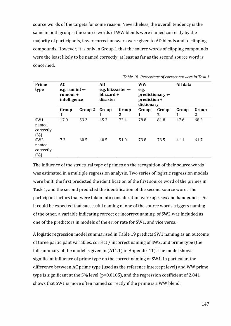
147

source words of the targets for some reason. Nevertheless, the overall tendency is the

same in both groups: the source words of WW blends were named correctly by the

majority of participants, fewer correct answers were given to AD blends and to clipping

compounds. However, it is only in Group 1 that the source words of clipping compounds

were the least likely to be named correctly, at least as far as the second source word is

concerned.

Table 18. Percentage of correct answers in Task 1

Prime type

AC e.g. rumint ← rumour + intelligence

AD e.g. blizzaster ← blizzard + disaster

WW e.g. predictionary ← prediction + dictionary

All data

Group 1

Group 2 Group 1

Group 2

Group 1

Group 2

Group 1

Group 2

SW1 named correctly (%)

17.0 53.2 45.2 72.4 78.8 81.8 47.6 68.2

SW2 named correctly (%)

7.3 60.5 40.5 51.0 73.8 73.5 41.1 61.7

The influence of the structural type of primes on the recognition of their source words

was estimated in a multiple regression analysis. Two series of logistic regression models

were built: the first predicted the identification of the first source word of the primes in

Task 1, and the second predicted the identification of the second source word. The

participant factors that were taken into consideration were age, sex and handedness. As

it could be expected that successful naming of one of the source words triggers naming

of the other, a variable indicating correct or incorrect naming of SW2 was included as

one of the predictors in models of the error rate for SW1, and vice versa.

A logistic regression model summarised in Table 19 predicts SW1 naming as an outcome

of three participant variables, correct / incorrect naming of SW2, and prime type (the

full summary of the model is given in (A11.1) in Appendix 11). The model shows

significant influence of prime type on the correct naming of SW1. In particular, the

difference between AC prime type (used as the reference intercept level) and WW prime

type is significant at the 5% level (p=0.0105), and the regression coefficient of 2.841

shows that SW1 is more often named correctly if the prime is a WW blend.

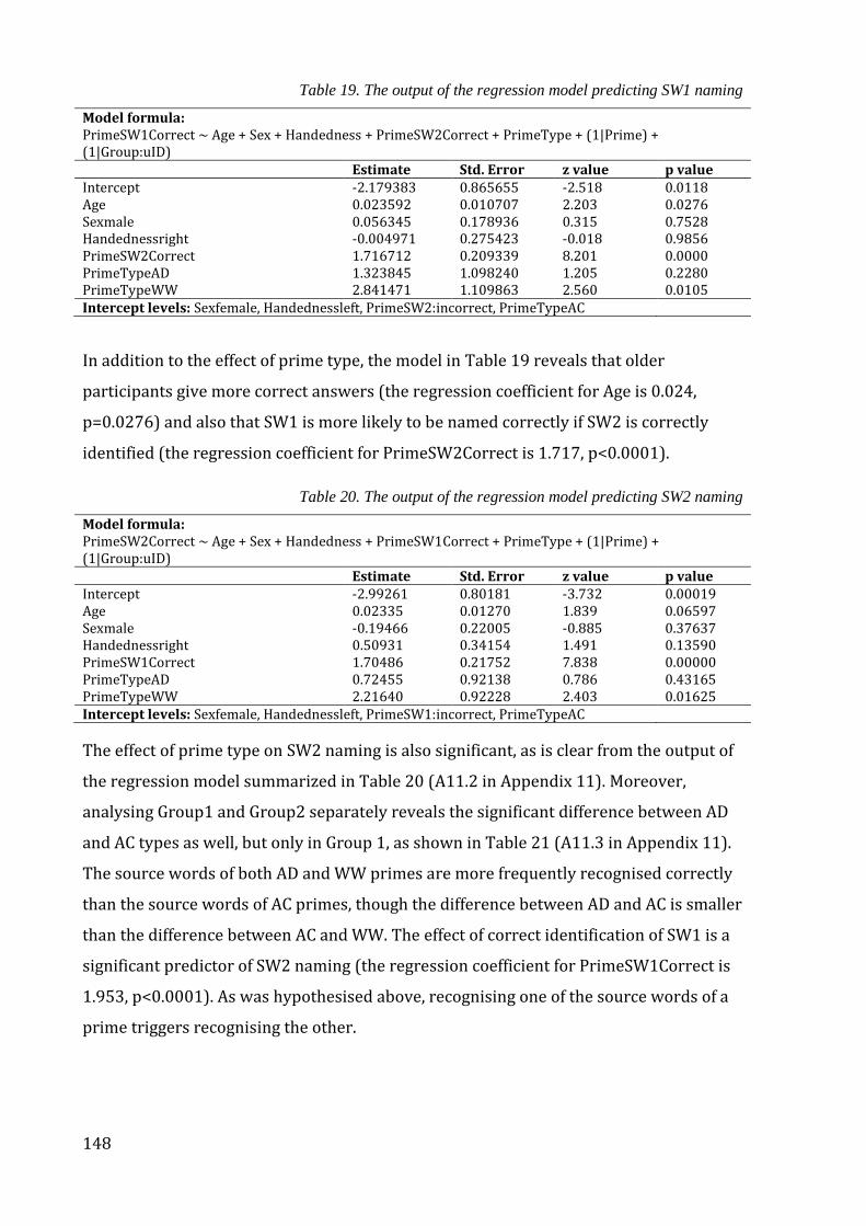
148

Table 19. The output of the regression model predicting SW1 naming

Model formula: PrimeSW1Correct ~ Age + Sex + Handedness + PrimeSW2Correct + PrimeType + (1|Prime) + (1|Group:uID) Estimate Std. Error z value p value Intercept -2.179383 0.865655 -2.518 0.0118 Age 0.023592 0.010707 2.203 0.0276 Sexmale 0.056345 0.178936 0.315 0.7528 Handednessright -0.004971 0.275423 -0.018 0.9856 PrimeSW2Correct 1.716712 0.209339 8.201 0.0000 PrimeTypeAD 1.323845 1.098240 1.205 0.2280 PrimeTypeWW 2.841471 1.109863 2.560 0.0105 Intercept levels: Sexfemale, Handednessleft, PrimeSW2:incorrect, PrimeTypeAC

In addition to the effect of prime type, the model in Table 19 reveals that older

participants give more correct answers (the regression coefficient for Age is 0.024,

p=0.0276) and also that SW1 is more likely to be named correctly if SW2 is correctly

identified (the regression coefficient for PrimeSW2Correct is 1.717, p<0.0001).

Table 20. The output of the regression model predicting SW2 naming

Model formula: PrimeSW2Correct ~ Age + Sex + Handedness + PrimeSW1Correct + PrimeType + (1|Prime) + (1|Group:uID) Estimate Std. Error z value p value Intercept -2.99261 0.80181 -3.732 0.00019 Age 0.02335 0.01270 1.839 0.06597 Sexmale -0.19466 0.22005 -0.885 0.37637 Handednessright 0.50931 0.34154 1.491 0.13590 PrimeSW1Correct 1.70486 0.21752 7.838 0.00000 PrimeTypeAD 0.72455 0.92138 0.786 0.43165 PrimeTypeWW 2.21640 0.92228 2.403 0.01625 Intercept levels: Sexfemale, Handednessleft, PrimeSW1:incorrect, PrimeTypeAC

The effect of prime type on SW2 naming is also significant, as is clear from the output of

the regression model summarized in Table 20 (A11.2 in Appendix 11). Moreover,

analysing Group1 and Group2 separately reveals the significant difference between AD

and AC types as well, but only in Group 1, as shown in Table 21 (A11.3 in Appendix 11).

The source words of both AD and WW primes are more frequently recognised correctly

than the source words of AC primes, though the difference between AD and AC is smaller

than the difference between AC and WW. The effect of correct identification of SW1 is a

significant predictor of SW2 naming (the regression coefficient for PrimeSW1Correct is

1.953, p<0.0001). As was hypothesised above, recognising one of the source words of a

prime triggers recognising the other.

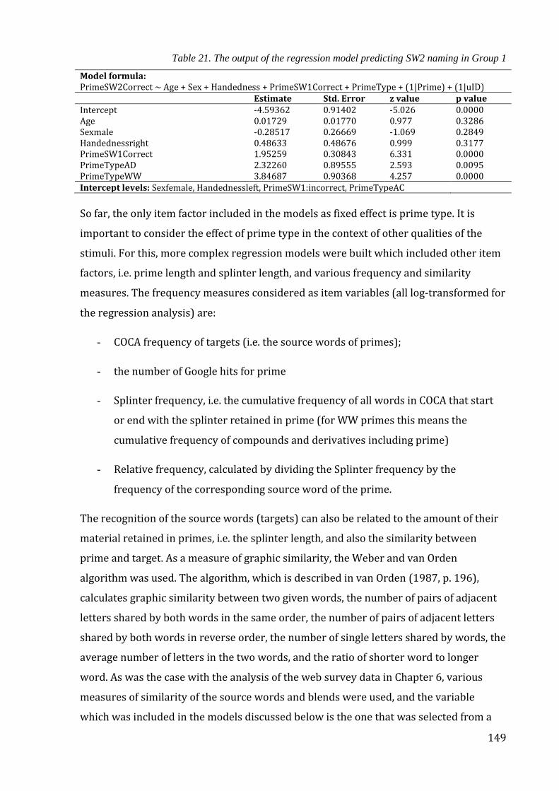
149

Table 21. The output of the regression model predicting SW2 naming in Group 1

Model formula: PrimeSW2Correct ~ Age + Sex + Handedness + PrimeSW1Correct + PrimeType + (1|Prime) + (1|uID) Estimate Std. Error z value p value Intercept -4.59362 0.91402 -5.026 0.0000 Age 0.01729 0.01770 0.977 0.3286 Sexmale -0.28517 0.26669 -1.069 0.2849 Handednessright 0.48633 0.48676 0.999 0.3177 PrimeSW1Correct 1.95259 0.30843 6.331 0.0000 PrimeTypeAD 2.32260 0.89555 2.593 0.0095 PrimeTypeWW 3.84687 0.90368 4.257 0.0000 Intercept levels: Sexfemale, Handednessleft, PrimeSW1:incorrect, PrimeTypeAC

So far, the only item factor included in the models as fixed effect is prime type. It is

important to consider the effect of prime type in the context of other qualities of the

stimuli. For this, more complex regression models were built which included other item

factors, i.e. prime length and splinter length, and various frequency and similarity

measures. The frequency measures considered as item variables (all log-transformed for

the regression analysis) are:

- COCA frequency of targets (i.e. the source words of primes);

- the number of Google hits for prime

- Splinter frequency, i.e. the cumulative frequency of all words in COCA that start

or end with the splinter retained in prime (for WW primes this means the

cumulative frequency of compounds and derivatives including prime)

- Relative frequency, calculated by dividing the Splinter frequency by the

frequency of the corresponding source word of the prime.

The recognition of the source words (targets) can also be related to the amount of their

material retained in primes, i.e. the splinter length, and also the similarity between

prime and target. As a measure of graphic similarity, the Weber and van Orden

algorithm was used. The algorithm, which is described in van Orden (1987, p. 196),

calculates graphic similarity between two given words, the number of pairs of adjacent

letters shared by both words in the same order, the number of pairs of adjacent letters

shared by both words in reverse order, the number of single letters shared by words, the

average number of letters in the two words, and the ratio of shorter word to longer

word. As was the case with the analysis of the web survey data in Chapter 6, various

measures of similarity of the source words and blends were used, and the variable

which was included in the models discussed below is the one that was selected from a

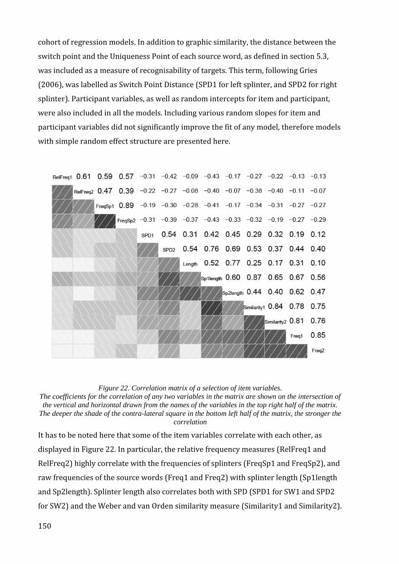
150

cohort of regression models. In addition to graphic similarity, the distance between the

switch point and the Uniqueness Point of each source word, as defined in section 5.3,

was included as a measure of recognisability of targets. This term, following Gries

(2006), was labelled as Switch Point Distance (SPD1 for left splinter, and SPD2 for right

splinter). Participant variables, as well as random intercepts for item and participant,

were also included in all the models. Including various random slopes for item and

participant variables did not significantly improve the fit of any model, therefore models

with simple random effect structure are presented here.

Figure 22. Correlation matrix of a selection of item variables.

The coefficients for the correlation of any two variables in the matrix are shown on the intersection of

the vertical and horizontal drawn from the names of the variables in the top right half of the matrix.

The deeper the shade of the contra-lateral square in the bottom left half of the matrix, the stronger the

correlation

It has to be noted here that some of the item variables correlate with each other, as

displayed in Figure 22. In particular, the relative frequency measures (RelFreq1 and

RelFreq2) highly correlate with the frequencies of splinters (FreqSp1 and FreqSp2), and

raw frequencies of the source words (Freq1 and Freq2) with splinter length (Sp1length

and Sp2length). Splinter length also correlates both with SPD (SPD1 for SW1 and SPD2

for SW2) and the Weber and van Orden similarity measure (Similarity1 and Similarity2).

151

On the one hand, an analysis of the systematic relations between these various

characteristics of blend words is an interesting subject in itself, and looking into these

relations might prove sensible, although would need a much larger lexical data sample

than the 30 words used for this experiment. On the other hand, multiple correlations

shown in Figure 22 are problematic for predicting the effect of these factors on the

probability of correct identification of targets, or on the reaction time (see, for example,

Baayen (2008) for a detailed discussion of the problem of multicollinearity caused by

such situations).

Table 22. Likelihood ratio tests comparing models with splinter frequency and relative frequency

predicting SW1 naming


Chi-square

Df for Chi-square

p-value

model including splinter frequency

9 1064.5 1112.6 -523.27

model including relative frequency

9 1048.1 1096.2 -515.07 16.395 0 <0.0001

One approach to multicollinearity is to select one variable out of a cluster of correlating

predictors. This method is appropriate in our case because some of the variables

discussed here are different ways of estimating the same property. For example, splinter

frequency is built into relative frequency by the way relative frequency is calculated.

Such variables as similarity, splinter length and SPD are all related to the degree of

preservation of the material of the source words in a blend. Therefore, a series of

regression models was built, each of the models including only one variable from each

cluster of correlating predictors. The full model predicting the number of correct

responses in the identification and production task was built in several steps. Firstly,

either splinter frequency (FreqSp) or relative splinter frequency (RelFreq) was selected

to account for the splinter frequency effect. The influence of splinter frequency on the

identification of source words was better grasped by the relative frequency variables,

which is true both for SW1 (as shown in Table 22) and SW2 naming (as shown in Table

23).

Table 23. Likelihood ratio tests comparing models with splinter frequency and relative frequency

predicting SW2 naming


Chi-square

Df for Chi-square

p-value

model including splinter frequency

9 1232.2 1280.3 -607.09

model including relative frequency

9 1230.0 1278.1 -606.01 2.1589 0 <0.0001

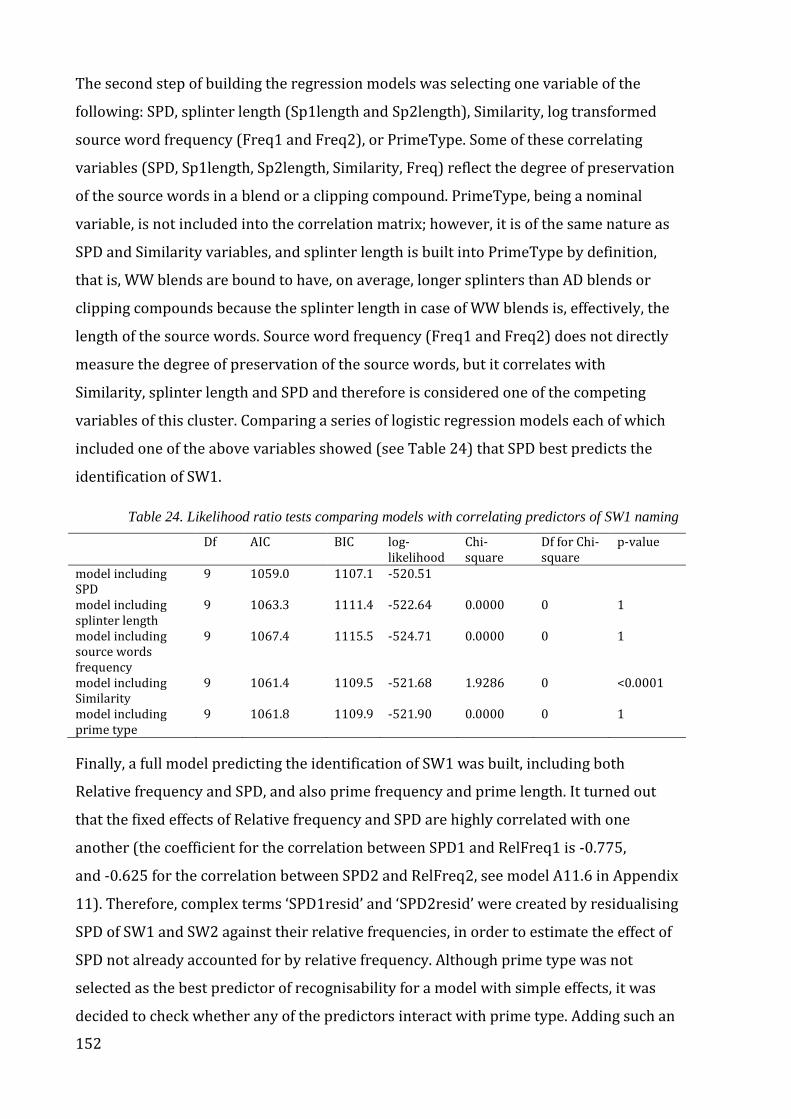
152

The second step of building the regression models was selecting one variable of the

following: SPD, splinter length (Sp1length and Sp2length), Similarity, log transformed

source word frequency (Freq1 and Freq2), or PrimeType. Some of these correlating

variables (SPD, Sp1length, Sp2length, Similarity, Freq) reflect the degree of preservation

of the source words in a blend or a clipping compound. PrimeType, being a nominal

variable, is not included into the correlation matrix; however, it is of the same nature as

SPD and Similarity variables, and splinter length is built into PrimeType by definition,

that is, WW blends are bound to have, on average, longer splinters than AD blends or

clipping compounds because the splinter length in case of WW blends is, effectively, the

length of the source words. Source word frequency (Freq1 and Freq2) does not directly

measure the degree of preservation of the source words, but it correlates with

Similarity, splinter length and SPD and therefore is considered one of the competing

variables of this cluster. Comparing a series of logistic regression models each of which

included one of the above variables showed (see Table 24) that SPD best predicts the

identification of SW1.

Table 24. Likelihood ratio tests comparing models with correlating predictors of SW1 naming


Chi-square

Df for Chi-square

p-value

model including SPD

9 1059.0 1107.1 -520.51

model including splinter length

9 1063.3 1111.4 -522.64 0.0000 0 1

model including source words frequency

9 1067.4 1115.5 -524.71 0.0000 0 1

model including Similarity

9 1061.4 1109.5 -521.68 1.9286 0 <0.0001

model including prime type

9 1061.8 1109.9 -521.90 0.0000 0 1

Finally, a full model predicting the identification of SW1 was built, including both

Relative frequency and SPD, and also prime frequency and prime length. It turned out

that the fixed effects of Relative frequency and SPD are highly correlated with one

another (the coefficient for the correlation between SPD1 and RelFreq1 is -0.775,

and -0.625 for the correlation between SPD2 and RelFreq2, see model A11.6 in Appendix

11). Therefore, complex terms ‘SPD1resid’ and ‘SPD2resid’ were created by residualising

SPD of SW1 and SW2 against their relative frequencies, in order to estimate the effect of

SPD not already accounted for by relative frequency. Although prime type was not

selected as the best predictor of recognisability for a model with simple effects, it was

decided to check whether any of the predictors interact with prime type. Adding such an

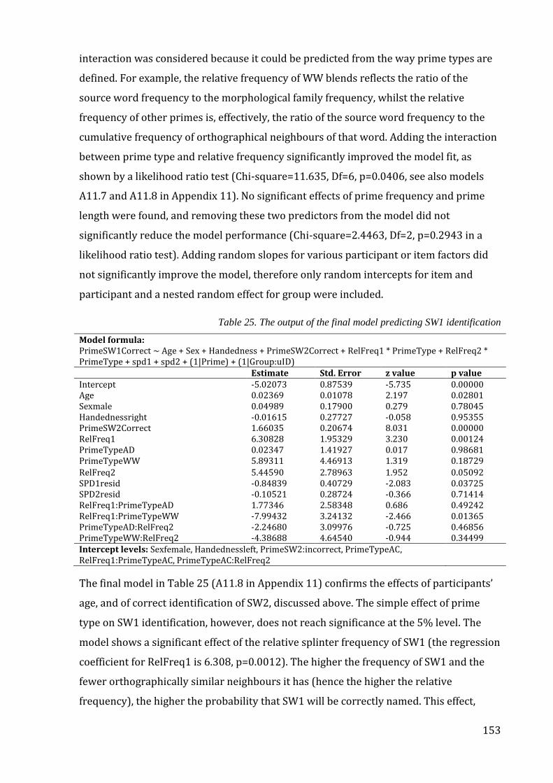
153

interaction was considered because it could be predicted from the way prime types are

defined. For example, the relative frequency of WW blends reflects the ratio of the

source word frequency to the morphological family frequency, whilst the relative

frequency of other primes is, effectively, the ratio of the source word frequency to the

cumulative frequency of orthographical neighbours of that word. Adding the interaction

between prime type and relative frequency significantly improved the model fit, as

shown by a likelihood ratio test (Chi-square=11.635, Df=6, p=0.0406, see also models

A11.7 and A11.8 in Appendix 11). No significant effects of prime frequency and prime

length were found, and removing these two predictors from the model did not

significantly reduce the model performance (Chi-square=2.4463, Df=2, p=0.2943 in a

likelihood ratio test). Adding random slopes for various participant or item factors did

not significantly improve the model, therefore only random intercepts for item and

participant and a nested random effect for group were included.

Table 25. The output of the final model predicting SW1 identification

Model formula: PrimeSW1Correct ~ Age + Sex + Handedness + PrimeSW2Correct + RelFreq1 * PrimeType + RelFreq2 * PrimeType + spd1 + spd2 + (1|Prime) + (1|Group:uID) Estimate Std. Error z value p value Intercept -5.02073 0.87539 -5.735 0.00000 Age 0.02369 0.01078 2.197 0.02801 Sexmale 0.04989 0.17900 0.279 0.78045 Handednessright -0.01615 0.27727 -0.058 0.95355 PrimeSW2Correct 1.66035 0.20674 8.031 0.00000 RelFreq1 6.30828 1.95329 3.230 0.00124 PrimeTypeAD 0.02347 1.41927 0.017 0.98681 PrimeTypeWW 5.89311 4.46913 1.319 0.18729

RelFreq2 5.44590 2.78963 1.952 0.05092 SPD1resid -0.84839 0.40729 -2.083 0.03725 SPD2resid -0.10521 0.28724 -0.366 0.71414 RelFreq1:PrimeTypeAD 1.77346 2.58348 0.686 0.49242 RelFreq1:PrimeTypeWW -7.99432 3.24132 -2.466 0.01365 PrimeTypeAD:RelFreq2 -2.24680 3.09976 -0.725 0.46856 PrimeTypeWW:RelFreq2 -4.38688 4.64540 -0.944 0.34499 Intercept levels: Sexfemale, Handednessleft, PrimeSW2:incorrect, PrimeTypeAC, RelFreq1:PrimeTypeAC, PrimeTypeAC:RelFreq2

The final model in Table 25 (A11.8 in Appendix 11) confirms the effects of participants’

age, and of correct identification of SW2, discussed above. The simple effect of prime

type on SW1 identification, however, does not reach significance at the 5% level. The

model shows a significant effect of the relative splinter frequency of SW1 (the regression

coefficient for RelFreq1 is 6.308, p=0.0012). The higher the frequency of SW1 and the

fewer orthographically similar neighbours it has (hence the higher the relative

frequency), the higher the probability that SW1 will be correctly named. This effect,

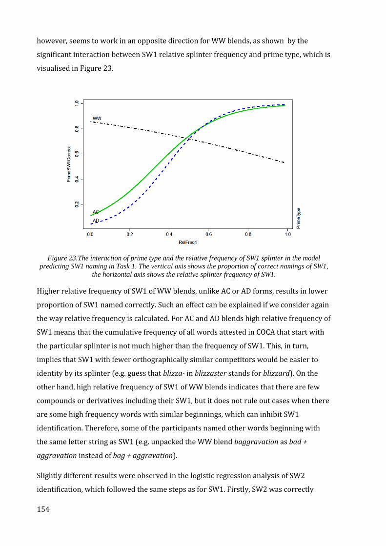
154

however, seems to work in an opposite direction for WW blends, as shown by the

significant interaction between SW1 relative splinter frequency and prime type, which is

visualised in Figure 23.

Figure 23.The interaction of prime type and the relative frequency of SW1 splinter in the model

predicting SW1 naming in Task 1. The vertical axis shows the proportion of correct namings of SW1,

the horizontal axis shows the relative splinter frequency of SW1.

Higher relative frequency of SW1 of WW blends, unlike AC or AD forms, results in lower

proportion of SW1 named correctly. Such an effect can be explained if we consider again

the way relative frequency is calculated. For AC and AD blends high relative frequency of

SW1 means that the cumulative frequency of all words attested in COCA that start with

the particular splinter is not much higher than the frequency of SW1. This, in turn,

implies that SW1 with fewer orthographically similar competitors would be easier to

identity by its splinter (e.g. guess that blizza- in blizzaster stands for blizzard). On the

other hand, high relative frequency of SW1 of WW blends indicates that there are few

compounds or derivatives including their SW1, but it does not rule out cases when there

are some high frequency words with similar beginnings, which can inhibit SW1

identification. Therefore, some of the participants named other words beginning with

the same letter string as SW1 (e.g. unpacked the WW blend baggravation as bad +

aggravation instead of bag + aggravation).

Slightly different results were observed in the logistic regression analysis of SW2

identification, which followed the same steps as for SW1. Firstly, SW2 was correctly

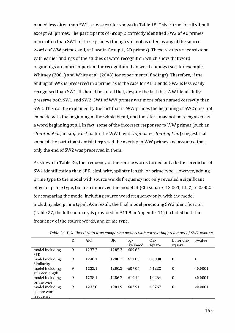
155

named less often than SW1, as was earlier shown in Table 18. This is true for all stimuli

except AC primes. The participants of Group 2 correctly identified SW2 of AC primes

more often than SW1 of those primes (though still not as often as any of the source

words of WW primes and, at least in Group 1, AD primes). These results are consistent

with earlier findings of the studies of word recognition which show that word

beginnings are more important for recognition than word endings (see, for example,

Whitney (2001) and White et al. (2008) for experimental findings). Therefore, if the

ending of SW2 is preserved in a prime, as is the case for AD blends, SW2 is less easily

recognised than SW1. It should be noted that, despite the fact that WW blends fully

preserve both SW1 and SW2, SW1 of WW primes was more often named correctly than

SW2. This can be explained by the fact that in WW primes the beginning of SW2 does not

coincide with the beginning of the whole blend, and therefore may not be recognised as

a word beginning at all. In fact, some of the incorrect responses to WW primes (such as

stop + motion, or stop + action for the WW blend stoption ← stop + option) suggest that

some of the participants misinterpreted the overlap in WW primes and assumed that

only the end of SW2 was preserved in them.

As shown in Table 26, the frequency of the source words turned out a better predictor of

SW2 identification than SPD, similarity, splinter length, or prime type. However, adding

prime type to the model with source words frequency not only revealed a significant

effect of prime type, but also improved the model fit (Chi square=12.001, Df=2, p=0.0025

for comparing the model including source word frequency only, with the model

including also prime type). As a result, the final model predicting SW2 identification

(Table 27, the full summary is provided in A11.9 in Appendix 11) included both the

frequency of the source words, and prime type.

Table 26. Likelihood ratio tests comparing models with correlating predictors of SW2 naming


Chi-square

Df for Chi-square

p-value

model including SPD

9 1237.2 1285.3 -609.62

model including Similarity

9 1240.1 1288.3 -611.06 0.0000 0 1

model including splinter length

9 1232.1 1280.2 -607.06 5.1222 0 <0.0001

model including prime type

9 1238.1 1286.3 -610.10 1.9264 0 <0.0001

model including source word frequency

9 1233.8 1281.9 -607.91 4.3767 0 <0.0001

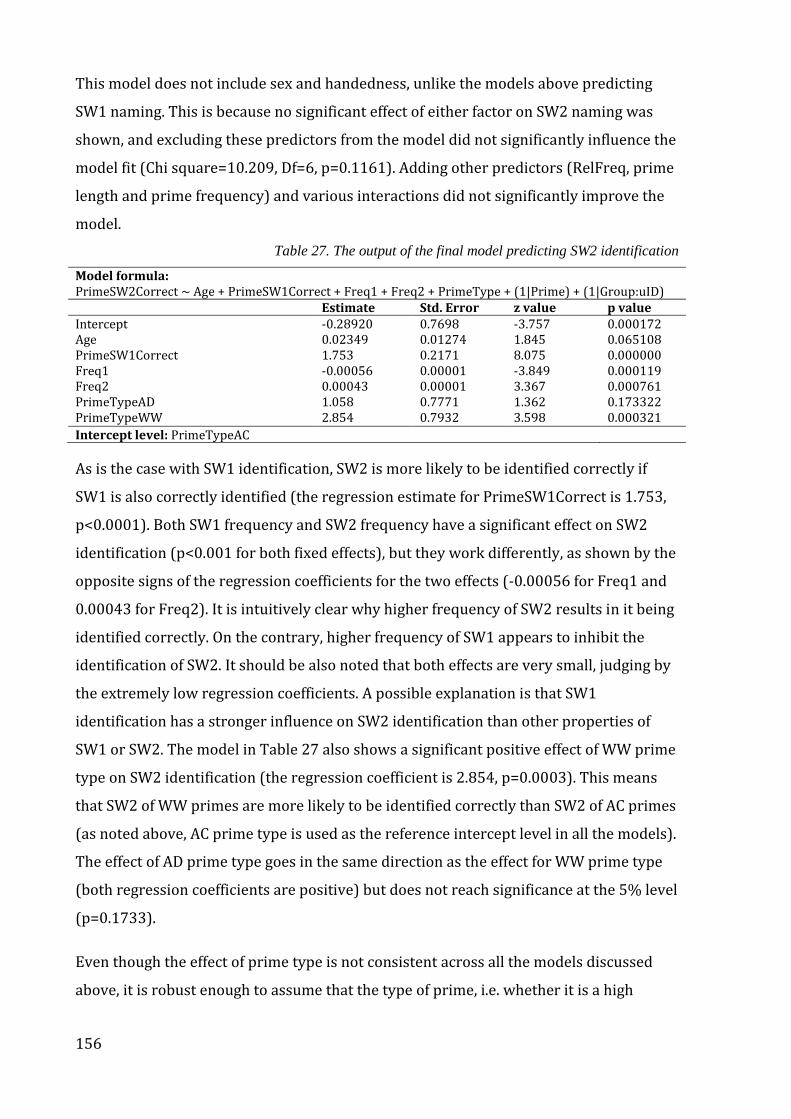
156

This model does not include sex and handedness, unlike the models above predicting

SW1 naming. This is because no significant effect of either factor on SW2 naming was

shown, and excluding these predictors from the model did not significantly influence the

model fit (Chi square=10.209, Df=6, p=0.1161). Adding other predictors (RelFreq, prime

length and prime frequency) and various interactions did not significantly improve the

model.

Table 27. The output of the final model predicting SW2 identification

Model formula: PrimeSW2Correct ~ Age + PrimeSW1Correct + Freq1 + Freq2 + PrimeType + (1|Prime) + (1|Group:uID) Estimate Std. Error z value p value Intercept -0.28920 0.7698 -3.757 0.000172 Age 0.02349 0.01274 1.845 0.065108 PrimeSW1Correct 1.753 0.2171 8.075 0.000000 Freq1 -0.00056 0.00001 -3.849 0.000119 Freq2 0.00043 0.00001 3.367 0.000761 PrimeTypeAD 1.058 0.7771 1.362 0.173322 PrimeTypeWW 2.854 0.7932 3.598 0.000321

Intercept level: PrimeTypeAC

As is the case with SW1 identification, SW2 is more likely to be identified correctly if

SW1 is also correctly identified (the regression estimate for PrimeSW1Correct is 1.753,

p<0.0001). Both SW1 frequency and SW2 frequency have a significant effect on SW2

identification (p<0.001 for both fixed effects), but they work differently, as shown by the

opposite signs of the regression coefficients for the two effects (-0.00056 for Freq1 and

0.00043 for Freq2). It is intuitively clear why higher frequency of SW2 results in it being

identified correctly. On the contrary, higher frequency of SW1 appears to inhibit the

identification of SW2. It should be also noted that both effects are very small, judging by

the extremely low regression coefficients. A possible explanation is that SW1

identification has a stronger influence on SW2 identification than other properties of

SW1 or SW2. The model in Table 27 also shows a significant positive effect of WW prime

type on SW2 identification (the regression coefficient is 2.854, p=0.0003). This means

that SW2 of WW primes are more likely to be identified correctly than SW2 of AC primes

(as noted above, AC prime type is used as the reference intercept level in all the models).

The effect of AD prime type goes in the same direction as the effect for WW prime type

(both regression coefficients are positive) but does not reach significance at the 5% level

(p=0.1733).

Even though the effect of prime type is not consistent across all the models discussed

above, it is robust enough to assume that the type of prime, i.e. whether it is a high

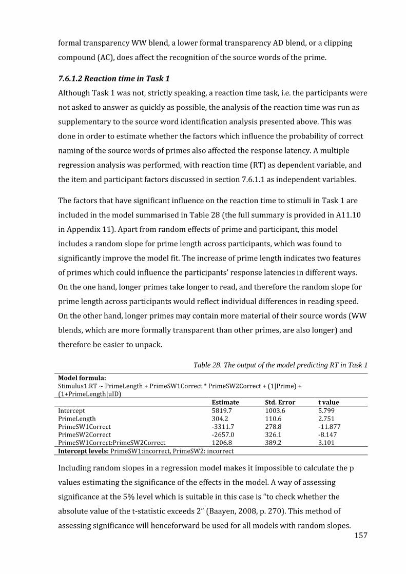
157

formal transparency WW blend, a lower formal transparency AD blend, or a clipping

compound (AC), does affect the recognition of the source words of the prime.

7.6.1.2 Reaction time in Task 1

Although Task 1 was not, strictly speaking, a reaction time task, i.e. the participants were

not asked to answer as quickly as possible, the analysis of the reaction time was run as

supplementary to the source word identification analysis presented above. This was

done in order to estimate whether the factors which influence the probability of correct

naming of the source words of primes also affected the response latency. A multiple

regression analysis was performed, with reaction time (RT) as dependent variable, and

the item and participant factors discussed in section 7.6.1.1 as independent variables.

The factors that have significant influence on the reaction time to stimuli in Task 1 are

included in the model summarised in Table 28 (the full summary is provided in A11.10

in Appendix 11). Apart from random effects of prime and participant, this model

includes a random slope for prime length across participants, which was found to

significantly improve the model fit. The increase of prime length indicates two features

of primes which could influence the participants’ response latencies in different ways.

On the one hand, longer primes take longer to read, and therefore the random slope for

prime length across participants would reflect individual differences in reading speed.

On the other hand, longer primes may contain more material of their source words (WW

blends, which are more formally transparent than other primes, are also longer) and

therefore be easier to unpack.

Table 28. The output of the model predicting RT in Task 1

Model formula: Stimulus1.RT ~ PrimeLength + PrimeSW1Correct * PrimeSW2Correct + (1|Prime) + (1+PrimeLength|uID) Estimate Std. Error t value Intercept 5819.7 1003.6 5.799 PrimeLength 304.2 110.6 2.751 PrimeSW1Correct -3311.7 278.8 -11.877 PrimeSW2Correct -2657.0 326.1 -8.147 PrimeSW1Correct:PrimeSW2Correct 1206.8 389.2 3.101 Intercept levels: PrimeSW1:incorrect, PrimeSW2: incorrect

Including random slopes in a regression model makes it impossible to calculate the p

values estimating the significance of the effects in the model. A way of assessing

significance at the 5% level which is suitable in this case is “to check whether the

absolute value of the t-statistic exceeds 2” (Baayen, 2008, p. 270). This method of

assessing significance will henceforward be used for all models with random slopes.

158

The model in Table 28 shows that it takes longer to identify the source words in longer

primes (hence the positive value of the regression coefficient for prime length). The

model also includes negative separate effects of the correct identification of SW1 and

SW2 on the RT, which indicate that it takes less time for the participants to give their

answer if they correctly identify either SW1 or SW2. This is also true for cases when

both SW1 and SW2 are named correctly, but the positive regression coefficient for the

interaction of these two factors shows that these effects are not simply additive. The

model shows that the participants who name both SW1 and SW2 correctly tend to

answer faster but not as fast one would expect if SW1 and SW2 were acting completely

independently of each other, which is most likely a floor effect.

As is clear from the analysis above, although the structural type of prime appears to

influence the identification of targets, it does not affect the speed of response. The

following section discusses whether the type of prime influences the recognition of

targets in a subsequent lexical decision task.

7.6.2. Lexical decision task results

As mentioned in section 7.5, the primary focus of the analysis of the lexical decision task

is on the reaction time. An analysis of errors will also be presented in addition to the RT

analysis.

7.6.2.1. Reaction time analysis

The RT analysis is based on responses from 103 participants whose overall error rate in

Task 2 is smaller than 20%. Incorrect answers (i.e. pressing the NO button for word

stimuli or YES answers to pseudoword stimuli, making up 4.5% of all responses to word

stimuli and 8.7% of responses to pseudoword stimuli) are also excluded from the

analysis. A lower response threshold of 200 ms was set, but no responses were faster

than this. On the other hand, about 3% of responses were more than 2.5 SD above the

overall mean RT. On studying the distribution of RT it was decided, however, to keep the

slow responses in the data set. The reason they cannot be simply discarded as outliers is

that the responses are not normally distributed, as illustrated in the density plot in

Figure 24. The strong right skew of the distribution reflects the large number of slow

responses observed in the data.

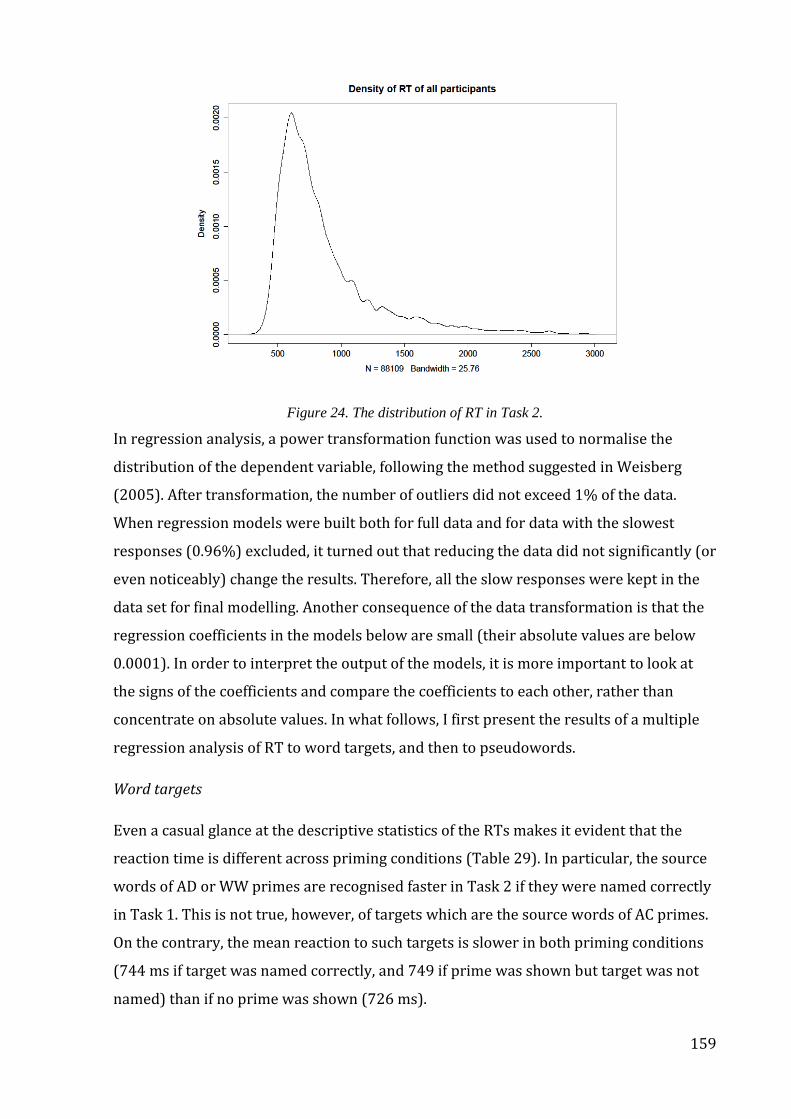
159

Figure 24. The distribution of RT in Task 2.

In regression analysis, a power transformation function was used to normalise the

distribution of the dependent variable, following the method suggested in Weisberg

(2005). After transformation, the number of outliers did not exceed 1% of the data.

When regression models were built both for full data and for data with the slowest

responses (0.96%) excluded, it turned out that reducing the data did not significantly (or

even noticeably) change the results. Therefore, all the slow responses were kept in the

data set for final modelling. Another consequence of the data transformation is that the

regression coefficients in the models below are small (their absolute values are below

0.0001). In order to interpret the output of the models, it is more important to look at

the signs of the coefficients and compare the coefficients to each other, rather than

concentrate on absolute values. In what follows, I first present the results of a multiple

regression analysis of RT to word targets, and then to pseudowords.

Word targets

Even a casual glance at the descriptive statistics of the RTs makes it evident that the

reaction time is different across priming conditions (Table 29). In particular, the source

words of AD or WW primes are recognised faster in Task 2 if they were named correctly

in Task 1. This is not true, however, of targets which are the source words of AC primes.

On the contrary, the mean reaction to such targets is slower in both priming conditions

(744 ms if target was named correctly, and 749 if prime was shown but target was not

named) than if no prime was shown (726 ms).

160

Table 29. Mean reaction time to target words in Task 2 for different priming conditions, millisecs (SD)

Priming condition Prime shown in Task 1, and target named correctly

Prime shown in Task 1, and target not named correctly

No prime

AC prime AD prime WW prime All words

744 (292) 682 (244) 683 (235) 704 (260)

749 (275) 703 (271) 703 (237) 718 (262)

726 (260) 705 (278) 726 (267) 719 (269)

The effect of both prime type and priming condition (i.e. whether the prime was shown

in Task 1 or not, and whether the target was named) on the response latency in the

lexical decision task was explored in multiple regression analysis. The regression

models presented below include the same participant variables as the models in section

7.6.1. The item variables used for the analysis were selected and labelled in a different

way, accounting for the fact that two targets can share the same prime. The following

item variables were used for the regression analysis (the full list of abbreviations for

item variables is given in Appendix 10):

– log transformed Google frequency of prime (LogPfreq);

– log transformed COCA frequency of the target (LogTfreq);

– relative splinter frequency of the corresponding splinter of prime (Prelfreq),

calculated as the cumulative frequency of words beginning or ending with the

splinter divided by the frequency of the target, using the method suggested in

Cook and Stevenson (2007);

– similarity between target and prime (Weber and van Orden (1987) spelling

distance between target and prime, labelled as Similarity);

– SPD between prime and target (Pspd):

– prime length (Plength);

– target length (Tlength);

– Splinter length (SpLength);

– prime type (AC, AD or WW)

The effect of the exposure to primes in Task 1 on the response latency is revealed in the

regression model displayed in Table 30 (the full summary of the model is given in

A11.11 in Appendix 11). Judging by the negative regression coefficient (-0.00001079)

for PrimeShownTRUE variable, RT in Task 2 decreases (i.e. the recognition of targets is

facilitated) if the prime was shown in Task 1. On the other hand, no significant effect of

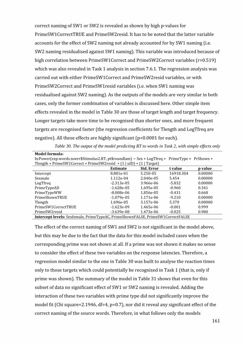
161

correct naming of SW1 or SW2 is revealed as shown by high p-values for

PrimeSW1CorrectTRUE and PrimeSW2resid. It has to be noted that the latter variable

accounts for the effect of SW2 naming not already accounted for by SW1 naming (i.e.

SW2 naming residualised against SW1 naming). This variable was introduced because of

high correlation between PrimeSW1Correct and PrimeSW2Correct variables (r=0.519)

which was also revealed in Task 1 analysis in section 7.6.1. The regression analysis was

carried out with either PrimeSW1Correct and PrimeSW2resid variables, or with

PrimeSW2Correct and PrimeSW1resid variables (i.e. when SW1 naming was

residualised against SW2 naming). As the outputs of the models are very similar in both

cases, only the former combination of variables is discussed here. Other simple item

effects revealed in the model in Table 30 are those of target length and target frequency.

Longer targets take more time to be recognised than shorter ones, and more frequent

targets are recognised faster (the regression coefficients for Tlength and LogTfreq are

negative). All these effects are highly significant (p<0.0001 for each).

Table 30. The output of the model predicting RT to words in Task 2, with simple effects only

Model formula: bcPower(exp.words.noerr$Stimulus2.RT, pt$roundlam) ~ Sex + LogTfreq + PrimeType + PrShown + Tlength + PrimeSW1Correct + PrimeSW2resid + (1 | uID) + (1 | Target) Estimate Std. Error t value p value Intercept 8.881e-01 5.250-05 16918.304 0.00000 Sexmale 1.112e-04 2.040e-05 5.454 0.00000 LogTfreq -2.313e-05 3.966e-06 -5.832 0.00000 PrimeTypeAD -1.628e-05 1.695e-05 -0.960 0.341 PrimeTypeWW -8.008e-06 1.856e-05 -0.431 0.668 PrimeShownTRUE -1.079e-05 1.171e-06 -9.210 0.00000 Tlength 1.696e-05 3.157e-06 5.370 0.00000 PrimeSW1CorrectTRUE -1.623e-09 1.465e-06 -0.001 0.999 PrimeSW2resid -3.639e-08 1.473e-06 -0.025 0.980 Intercept levels: Sexfemale, PrimeTypeAC, PrimeShownFALSE, PrimeSW1CorrectFALSE

The effect of the correct naming of SW1 and SW2 is not significant in the model above,

but this may be due to the fact that the data for this model included cases when the

corresponding prime was not shown at all. If a prime was not shown it makes no sense

to consider the effect of these two variables on the response latencies. Therefore, a

regression model similar to the one in Table 30 was built to analyse the reaction times

only to those targets which could potentially be recognised in Task 1 (that is, only if

prime was shown). The summary of the model in Table 31 shows that even for this

subset of data no significant effect of SW1 or SW2 naming is revealed. Adding the

interaction of these two variables with prime type did not significantly improve the

model fit (Chi square=2.1946, df=4, p=0.7), nor did it reveal any significant effect of the

correct naming of the source words. Therefore, in what follows only the models

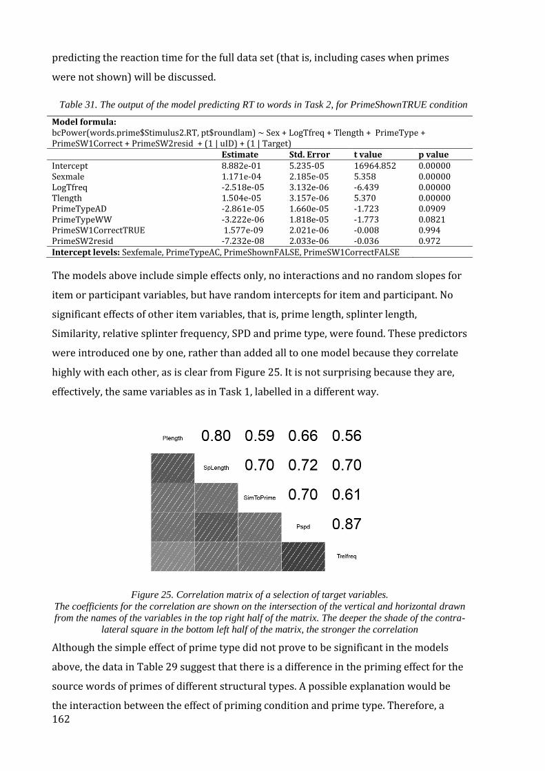
162

predicting the reaction time for the full data set (that is, including cases when primes

were not shown) will be discussed.

Table 31. The output of the model predicting RT to words in Task 2, for PrimeShownTRUE condition

Model formula: bcPower(words.prime$Stimulus2.RT, pt$roundlam) ~ Sex + LogTfreq + Tlength + PrimeType + PrimeSW1Correct + PrimeSW2resid + (1 | uID) + (1 | Target) Estimate Std. Error t value p value Intercept 8.882e-01 5.235-05 16964.852 0.00000 Sexmale 1.171e-04 2.185e-05 5.358 0.00000 LogTfreq -2.518e-05 3.132e-06 -6.439 0.00000 Tlength 1.504e-05 3.157e-06 5.370 0.00000 PrimeTypeAD -2.861e-05 1.660e-05 -1.723 0.0909 PrimeTypeWW -3.222e-06 1.818e-05 -1.773 0.0821 PrimeSW1CorrectTRUE 1.577e-09 2.021e-06 -0.008 0.994 PrimeSW2resid -7.232e-08 2.033e-06 -0.036 0.972 Intercept levels: Sexfemale, PrimeTypeAC, PrimeShownFALSE, PrimeSW1CorrectFALSE

The models above include simple effects only, no interactions and no random slopes for

item or participant variables, but have random intercepts for item and participant. No

significant effects of other item variables, that is, prime length, splinter length,

Similarity, relative splinter frequency, SPD and prime type, were found. These predictors

were introduced one by one, rather than added all to one model because they correlate

highly with each other, as is clear from Figure 25. It is not surprising because they are,

effectively, the same variables as in Task 1, labelled in a different way.

Figure 25. Correlation matrix of a selection of target variables.

The coefficients for the correlation are shown on the intersection of the vertical and horizontal drawn

from the names of the variables in the top right half of the matrix. The deeper the shade of the contra-

lateral square in the bottom left half of the matrix, the stronger the correlation

Although the simple effect of prime type did not prove to be significant in the models

above, the data in Table 29 suggest that there is a difference in the priming effect for the

source words of primes of different structural types. A possible explanation would be

the interaction between the effect of priming condition and prime type. Therefore, a

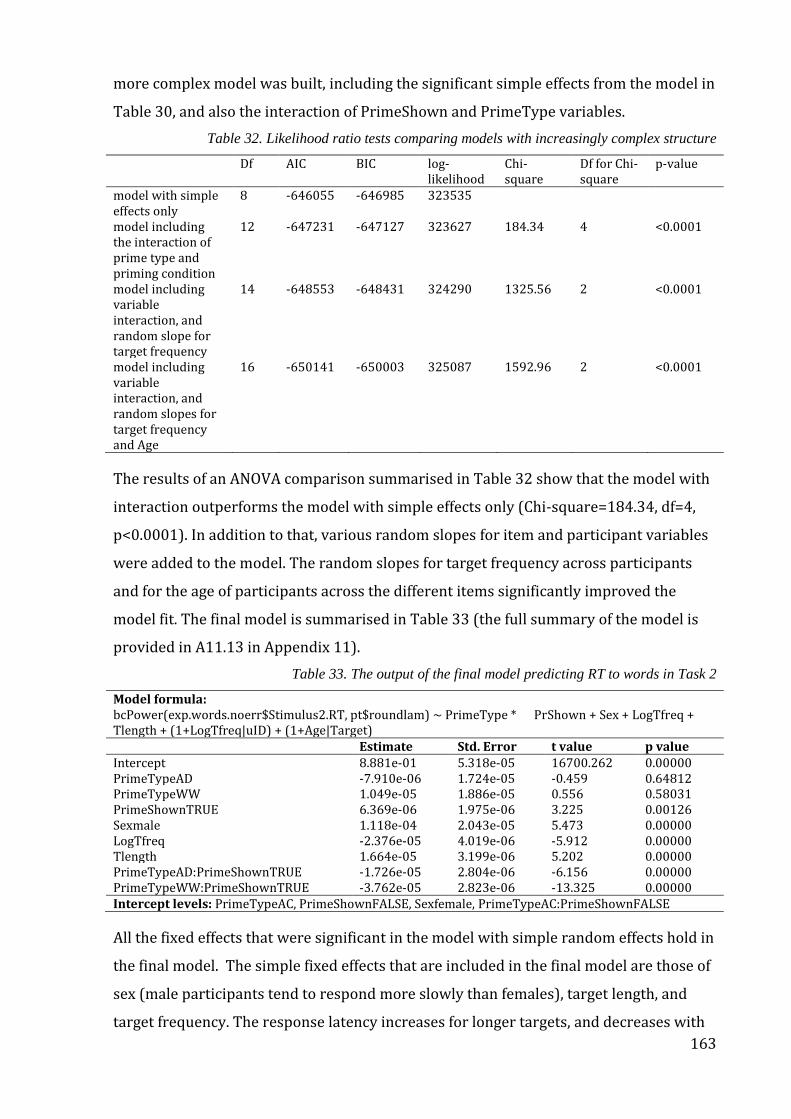
163

more complex model was built, including the significant simple effects from the model in

Table 30, and also the interaction of PrimeShown and PrimeType variables.



Chi-square

Df for Chi-square

p-value

model with simple effects only

8 -646055 -646985 323535

model including the interaction of prime type and priming condition

12 -647231 -647127 323627 184.34 4 <0.0001

model including variable interaction, and random slope for target frequency

14 -648553 -648431 324290 1325.56 2 <0.0001

model including variable interaction, and random slopes for target frequency and Age

16 -650141 -650003 325087 1592.96 2 <0.0001

The results of an ANOVA comparison summarised in Table 32 show that the model with

interaction outperforms the model with simple effects only (Chi-square=184.34, df=4,

p<0.0001). In addition to that, various random slopes for item and participant variables

were added to the model. The random slopes for target frequency across participants

and for the age of participants across the different items significantly improved the

model fit. The final model is summarised in Table 33 (the full summary of the model is

provided in A11.13 in Appendix 11).

Table 33. The output of the final model predicting RT to words in Task 2

Model formula: bcPower(exp.words.noerr$Stimulus2.RT, pt$roundlam) ~ PrimeType * PrShown + Sex + LogTfreq + Tlength + (1+LogTfreq|uID) + (1+Age|Target) Estimate Std. Error t value p value Intercept 8.881e-01 5.318e-05 16700.262 0.00000 PrimeTypeAD -7.910e-06 1.724e-05 -0.459 0.64812 PrimeTypeWW 1.049e-05 1.886e-05 0.556 0.58031 PrimeShownTRUE 6.369e-06 1.975e-06 3.225 0.00126 Sexmale 1.118e-04 2.043e-05 5.473 0.00000 LogTfreq -2.376e-05 4.019e-06 -5.912 0.00000 Tlength 1.664e-05 3.199e-06 5.202 0.00000 PrimeTypeAD:PrimeShownTRUE -1.726e-05 2.804e-06 -6.156 0.00000 PrimeTypeWW:PrimeShownTRUE -3.762e-05 2.823e-06 -13.325 0.00000 Intercept levels: PrimeTypeAC, PrimeShownFALSE, Sexfemale, PrimeTypeAC:PrimeShownFALSE

All the fixed effects that were significant in the model with simple random effects hold in

the final model. The simple fixed effects that are included in the final model are those of

sex (male participants tend to respond more slowly than females), target length, and

target frequency. The response latency increases for longer targets, and decreases with

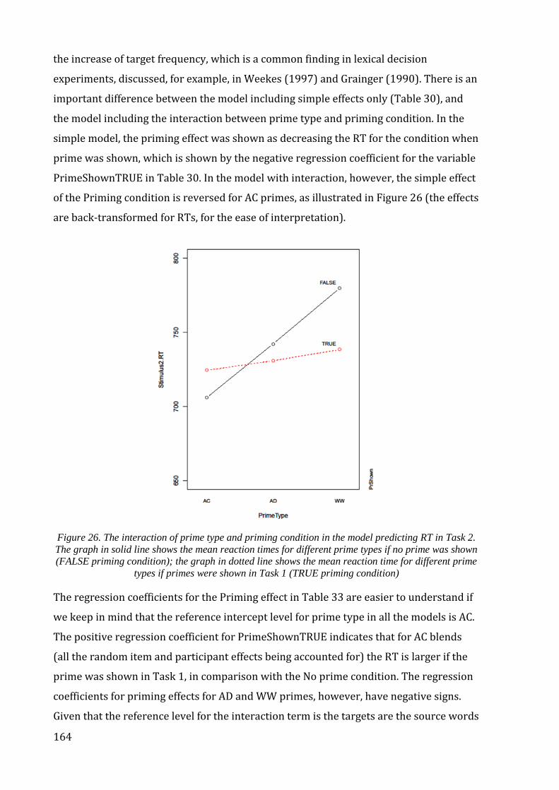
164

the increase of target frequency, which is a common finding in lexical decision

experiments, discussed, for example, in Weekes (1997) and Grainger (1990). There is an

important difference between the model including simple effects only (Table 30), and

the model including the interaction between prime type and priming condition. In the

simple model, the priming effect was shown as decreasing the RT for the condition when

prime was shown, which is shown by the negative regression coefficient for the variable

PrimeShownTRUE in Table 30. In the model with interaction, however, the simple effect

of the Priming condition is reversed for AC primes, as illustrated in Figure 26 (the effects

are back-transformed for RTs, for the ease of interpretation).

Figure 26. The interaction of prime type and priming condition in the model predicting RT in Task 2.

The graph in solid line shows the mean reaction times for different prime types if no prime was shown

(FALSE priming condition); the graph in dotted line shows the mean reaction time for different prime

types if primes were shown in Task 1 (TRUE priming condition)

The regression coefficients for the Priming effect in Table 33 are easier to understand if

we keep in mind that the reference intercept level for prime type in all the models is AC.

The positive regression coefficient for PrimeShownTRUE indicates that for AC blends

(all the random item and participant effects being accounted for) the RT is larger if the

prime was shown in Task 1, in comparison with the No prime condition. The regression

coefficients for priming effects for AD and WW primes, however, have negative signs.

Given that the reference level for the interaction term is the targets are the source words

165

of AC primes, with no primes shown in Task 1, this means that the response to the

source words of AD and WW primes in Task 2 (if the primes were shown in Task 1) is

significantly faster than the response to the source words of AC primes for which no

primes were shown. Moreover, the model in Table 33 confirms that both AD primes and

WW primes are significantly different from AC in this respect (p<0.0001 both for

PrimeShownTRUE:AD and PrimeShownTRUE:WW). The partial effects of prime type

and priming condition plotted in Figure 26 suggest that the exposure to AD and WW

Primes in Task 1 results in faster recognition of Targets in Task 2.

The facilitating effect of exposure to AD and WW primes on the recognition of Tagrets is

in agreement with Hypothesis 2 in section 7.1. As for AC primes, not only does prior

exposure to them not facilitate the recognition of their source words, but it also appears

to inhibit their recognition. The nature of this effect may become more evident if we look

at the recognition of nonword targets in the same task.

Nonword targets

Nonword targets created for Task 2 were matched with the word targets for syllabic

length and orthographic similarity to primes, as described in section 7.3. The mean

reaction time to nonword targets in the lexical decision task (987 ms) is higher than to

word targets (714 ms). This is consistent with earlier findings of many lexical decision

experiments, e.g. (Forster and Davis, 1984) which show that nonwords are generally

responded to more slowly than words. Partially this is because the NO button in this

experiment was pressed with the nondominant hand, but also because ‘non-acceptance’

judgements are generally slower than ‘acceptance’ judgements if the task is to determine

if a given letter string is a word (not to judge if it is a nonword).

Table 34. Mean reaction time to nonwords in Task 2, millisecs (SD)

Priming condition Prime shown in Task 1, and target word named correctly

Prime shown in Task 1, and target word not named correctly

No prime

AC prime AD prime WW prime All nonwords

1014 (475) 1016 (415) 934 (402) 987 (433)

1022 (463) 1010 (415) 977 (435) 1003 (439)

973 (430) 1012 (436) 911 (391) 964 (421)

What is interesting about the reaction to nonwords in this study is that the mean

reaction time is larger for nonwords orthographically similar to AC and WW primes if

the participants had seen the primes in Task 1. For nonwords similar to AD primes there

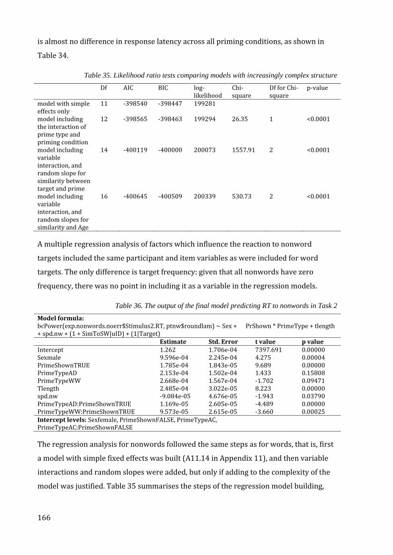
166

is almost no difference in response latency across all priming conditions, as shown in

Table 34.



Chi-square

Df for Chi-square

p-value

model with simple effects only

11 -398540 -398447 199281

model including the interaction of prime type and priming condition

12 -398565 -398463 199294 26.35 1 <0.0001

model including variable interaction, and random slope for similarity between target and prime

14 -400119 -400000 200073 1557.91 2 <0.0001

model including variable interaction, and random slopes for similarity and Age

16 -400645 -400509 200339 530.73 2 <0.0001

A multiple regression analysis of factors which influence the reaction to nonword

targets included the same participant and item variables as were included for word

targets. The only difference is target frequency: given that all nonwords have zero

frequency, there was no point in including it as a variable in the regression models.

Table 36. The output of the final model predicting RT to nonwords in Task 2

Model formula: bcPower(exp.nonwords.noerr$Stimulus2.RT, ptnw$roundlam) ~ Sex + PrShown * PrimeType + tlength + spd.nw + (1 + SimToSW|uID) + (1|Target) Estimate Std. Error t value p value Intercept 1.262 1.706e-04 7397.691 0.00000 Sexmale 9.596e-04 2.245e-04 4.275 0.00004 PrimeShownTRUE 1.785e-04 1.843e-05 9.689 0.00000 PrimeTypeAD 2.153e-04 1.502e-04 1.433 0.15808 PrimeTypeWW 2.668e-04 1.567e-04 -1.702 0.09471 Tlength 2.485e-04 3.022e-05 8.223 0.00000 spd.nw -9.084e-05 4.676e-05 -1.943 0.03790 PrimeTypeAD:PrimeShownTRUE 1.169e-05 2.605e-05 -4.489 0.00000 PrimeTypeWW:PrimeShownTRUE 9.573e-05 2.615e-05 -3.660 0.00025 Intercept levels: Sexfemale, PrimeShownFALSE, PrimeTypeAC, PrimeTypeAC:PrimeShownFALSE

The regression analysis for nonwords followed the same steps as for words, that is, first

a model with simple fixed effects was built (A11.14 in Appendix 11), and then variable

interactions and random slopes were added, but only if adding to the complexity of the

model was justified. Table 35 summarises the steps of the regression model building,

167

and the final model is shown in Table 36 (the full summary of the model is given in

A11.14 in Appendix 11).

Some factors appear to influence the response times for decisions made to nonword and

word targets in the same way. In particular, male participants react more slowly both to

word and nonword targets (hence the positive regression coefficients for Sexmale in the

model in Table 36, as well as in Table 33 above). Longer nonword targets take more

time to reject as not being words, as indicated by positive regression coefficient for

target length in Table 36. The main difference between the models predicting the

reaction time to word and nonword targets is in the direction and strength of the effect

of PrimeType, in interaction with the priming condition. Responses to nonword targets

orthographically similar to AD and WW primes were slower if the primes were shown in

Task 1. The main effect for PrimeShownTRUE variable also has a positive regression

coefficient. The regression analysis shows that responses to all nonwords were slower if

orthographically similar primes were shown in the task preceding the lexical decision.

However, the strength of this effect is different for different structural types of primes,

which is revealed by the significant effect of the interaction between prime type and

priming condition, as shown in Table 36.

Partial effects of prime type and priming condition in the models predicting RT for

words and nonwords are displayed in Figure 27. As it is clear from the left panel (which

shows the same effects as Figure 26 above), prior exposure to WW or AD primes

reduces the reaction time to their source words in the lexical decision task. The

facilitative effect is weaker for AD primes than for WW primes, and exposure to AC

primes results in slower reactions rather than faster ones. The right panel of the plot

demonstrates that prior exposure to primes slows down the reaction to targets, and this

is true for all three prime types, although the inhibitory effect of AD primes is smaller

than that of AC and WW primes.

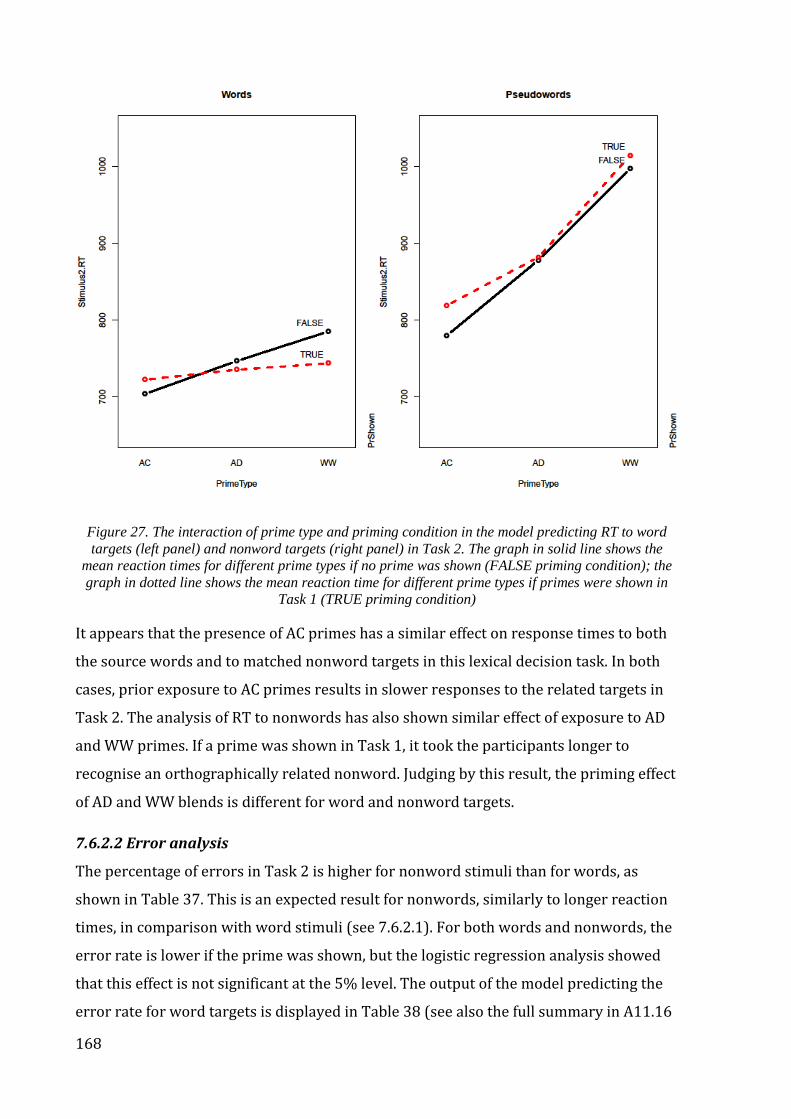
168

Figure 27. The interaction of prime type and priming condition in the model predicting RT to word

targets (left panel) and nonword targets (right panel) in Task 2. The graph in solid line shows the

mean reaction times for different prime types if no prime was shown (FALSE priming condition); the

graph in dotted line shows the mean reaction time for different prime types if primes were shown in

Task 1 (TRUE priming condition)

It appears that the presence of AC primes has a similar effect on response times to both

the source words and to matched nonword targets in this lexical decision task. In both

cases, prior exposure to AC primes results in slower responses to the related targets in

Task 2. The analysis of RT to nonwords has also shown similar effect of exposure to AD

and WW primes. If a prime was shown in Task 1, it took the participants longer to

recognise an orthographically related nonword. Judging by this result, the priming effect

of AD and WW blends is different for word and nonword targets.

7.6.2.2 Error analysis

The percentage of errors in Task 2 is higher for nonword stimuli than for words, as

shown in Table 37. This is an expected result for nonwords, similarly to longer reaction

times, in comparison with word stimuli (see 7.6.2.1). For both words and nonwords, the

error rate is lower if the prime was shown, but the logistic regression analysis showed

that this effect is not significant at the 5% level. The output of the model predicting the

error rate for word targets is displayed in Table 38 (see also the full summary in A11.16

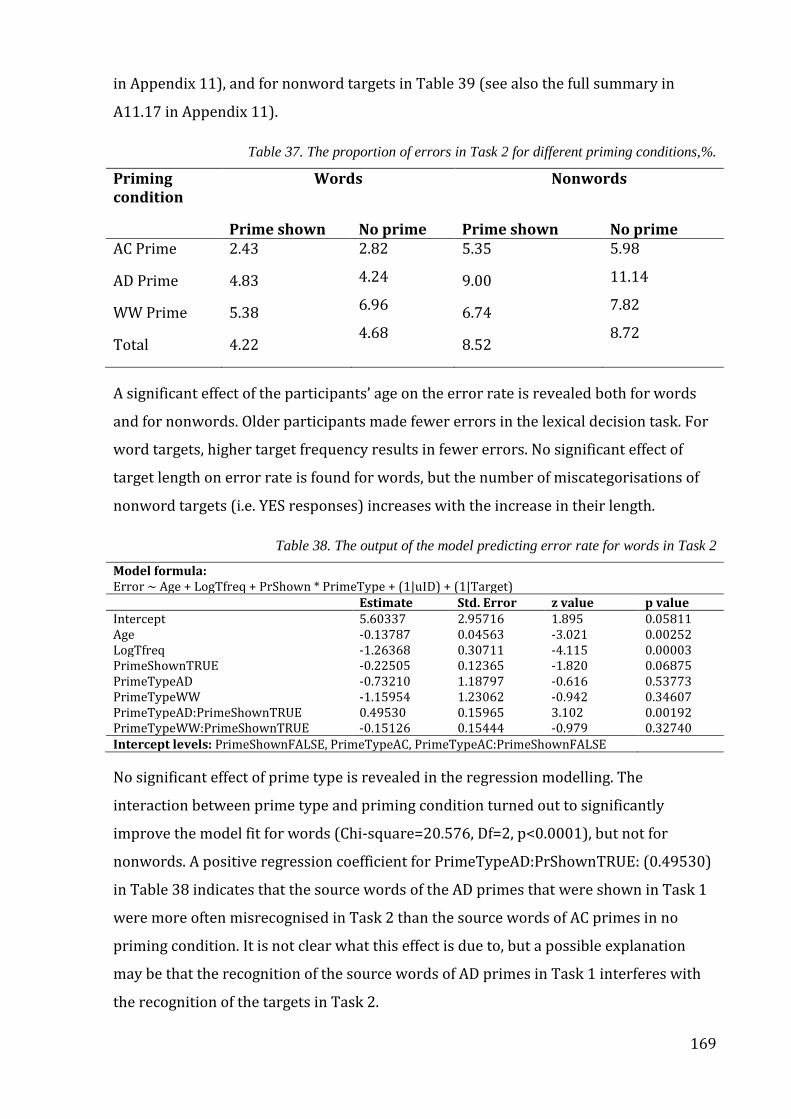
169

in Appendix 11), and for nonword targets in Table 39 (see also the full summary in

A11.17 in Appendix 11).

Table 37. The proportion of errors in Task 2 for different priming conditions,%.

Priming condition

Words Nonwords

Prime shown No prime Prime shown No prime AC Prime

AD Prime

WW Prime

Total

2.43

4.83

5.38

4.22

2.82

4.24

6.96

4.68

5.35

9.00

6.74

8.52

5.98

11.14

7.82

8.72

A significant effect of the participants’ age on the error rate is revealed both for words

and for nonwords. Older participants made fewer errors in the lexical decision task. For

word targets, higher target frequency results in fewer errors. No significant effect of

target length on error rate is found for words, but the number of miscategorisations of

nonword targets (i.e. YES responses) increases with the increase in their length.

Table 38. The output of the model predicting error rate for words in Task 2

Model formula: Error ~ Age + LogTfreq + PrShown * PrimeType + (1|uID) + (1|Target) Estimate Std. Error z value p value Intercept 5.60337 2.95716 1.895 0.05811 Age -0.13787 0.04563 -3.021 0.00252 LogTfreq -1.26368 0.30711 -4.115 0.00003 PrimeShownTRUE -0.22505 0.12365 -1.820 0.06875 PrimeTypeAD -0.73210 1.18797 -0.616 0.53773 PrimeTypeWW -1.15954 1.23062 -0.942 0.34607 PrimeTypeAD:PrimeShownTRUE 0.49530 0.15965 3.102 0.00192 PrimeTypeWW:PrimeShownTRUE -0.15126 0.15444 -0.979 0.32740 Intercept levels: PrimeShownFALSE, PrimeTypeAC, PrimeTypeAC:PrimeShownFALSE

No significant effect of prime type is revealed in the regression modelling. The

interaction between prime type and priming condition turned out to significantly

improve the model fit for words (Chi-square=20.576, Df=2, p<0.0001), but not for

nonwords. A positive regression coefficient for PrimeTypeAD:PrShownTRUE: (0.49530)

in Table 38 indicates that the source words of the AD primes that were shown in Task 1

were more often misrecognised in Task 2 than the source words of AC primes in no

priming condition. It is not clear what this effect is due to, but a possible explanation

may be that the recognition of the source words of AD primes in Task 1 interferes with

the recognition of the targets in Task 2.

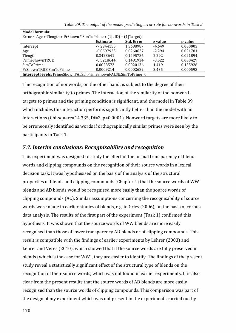
170

Table 39. The output of the model predicting error rate for nonwords in Task 2

Model formula: Error ~ Age + Tlength + PrShown * SimToPrime + (1|uID) + (1|Target) Estimate Std. Error z value p value Intercept -7.2944155 1.5688987 -4.649 0.000003 Age -0.0597923 0.0260627 -2.294 0.021781 Tlength 0.3428641 0.1495786 2.292 0.021894 PrimeShownTRUE -0.5218644 0.1481934 -3.522 0.000429 SimToPrime 0.0028572 0.0020136 1.419 0.155926 PrShownTRUE:SimToPrime 0.0009214 0.0002682 3.435 0.000593 Intercept levels: PrimeShownFALSE, PrimeShownFALSE:SimToPrime=0

The recognition of nonwords, on the other hand, is subject to the degree of their

orthographic similarity to primes. The interaction of the similarity of the nonword

targets to primes and the priming condition is significant, and the model in Table 39

which includes this interaction performs significantly better than the model with no

interactions (Chi-square=14.335, Df=2, p<0.0001). Nonword targets are more likely to

be erroneously identified as words if orthographically similar primes were seen by the

participants in Task 1.

7.7. Interim conclusions: Recognisability and recognition

This experiment was designed to study the effect of the formal transparency of blend

words and clipping compounds on the recognition of their source words in a lexical

decision task. It was hypothesised on the basis of the analysis of the structural

properties of blends and clipping compounds (Chapter 4) that the source words of WW

blends and AD blends would be recognised more easily than the source words of

clipping compounds (AC). Similar assumptions concerning the recognisability of source

words were made in earlier studies of blends, e.g. in Gries (2006), on the basis of corpus

data analysis. The results of the first part of the experiment (Task 1) confirmed this

hypothesis. It was shown that the source words of WW blends are more easily

recognised than those of lower transparency AD blends or of clipping compounds. This

result is compatible with the findings of earlier experiments by Lehrer (2003) and

Lehrer and Veres (2010), which showed that if the source words are fully preserved in

blends (which is the case for WW), they are easier to identify. The findings of the present

study reveal a statistically significant effect of the structural type of blends on the

recognition of their source words, which was not found in earlier experiments. It is also

clear from the present results that the source words of AD blends are more easily

recognised than the source words of clipping compounds. This comparison was part of

the design of my experiment which was not present in the experiments carried out by

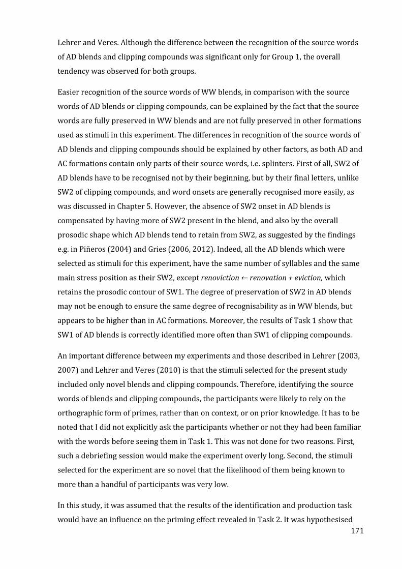
171

Lehrer and Veres. Although the difference between the recognition of the source words

of AD blends and clipping compounds was significant only for Group 1, the overall

tendency was observed for both groups.

Easier recognition of the source words of WW blends, in comparison with the source

words of AD blends or clipping compounds, can be explained by the fact that the source

words are fully preserved in WW blends and are not fully preserved in other formations

used as stimuli in this experiment. The differences in recognition of the source words of

AD blends and clipping compounds should be explained by other factors, as both AD and

AC formations contain only parts of their source words, i.e. splinters. First of all, SW2 of

AD blends have to be recognised not by their beginning, but by their final letters, unlike

SW2 of clipping compounds, and word onsets are generally recognised more easily, as

was discussed in Chapter 5. However, the absence of SW2 onset in AD blends is

compensated by having more of SW2 present in the blend, and also by the overall

prosodic shape which AD blends tend to retain from SW2, as suggested by the findings

e.g. in Piñeros (2004) and Gries (2006, 2012). Indeed, all the AD blends which were

selected as stimuli for this experiment, have the same number of syllables and the same

main stress position as their SW2, except renoviction ← renovation + eviction, which

retains the prosodic contour of SW1. The degree of preservation of SW2 in AD blends

may not be enough to ensure the same degree of recognisability as in WW blends, but

appears to be higher than in AC formations. Moreover, the results of Task 1 show that

SW1 of AD blends is correctly identified more often than SW1 of clipping compounds.

An important difference between my experiments and those described in Lehrer (2003,

2007) and Lehrer and Veres (2010) is that the stimuli selected for the present study

included only novel blends and clipping compounds. Therefore, identifying the source

words of blends and clipping compounds, the participants were likely to rely on the

orthographic form of primes, rather than on context, or on prior knowledge. It has to be

noted that I did not explicitly ask the participants whether or not they had been familiar

with the words before seeing them in Task 1. This was not done for two reasons. First,

such a debriefing session would make the experiment overly long. Second, the stimuli

selected for the experiment are so novel that the likelihood of them being known to

more than a handful of participants was very low.

In this study, it was assumed that the results of the identification and production task

would have an influence on the priming effect revealed in Task 2. It was hypothesised

172

that as a result of recognising the source words from blends in Task 1, the recognition of

the same source words in Task 2 would be facilitated. The results of Task 2 confirm the

priming effect of WW and AD blends on the recognition of their source words. It is also

confirmed that the priming effect is stronger for WW blends than for AD, as was

predicted. As for clipping compounds, no priming effect on the recognition of their

source words was predicted. The experiment results did not only show that, in

accordance with hypothesis 2, AC formations do not prime their source words, but they

also demonstrated that, in fact, there is an inhibitory effect of exposure to AC formations.

Such an effect is in line with the finding that the source words of AC formations were

most difficult to identify in Task 1. It was discussed in Chapter 5 that the source words of

AC are difficult to recognise because the splinters in AC formations are cut off too early

to reach the recognition point (as shown in Gries (2006) on the basis of corpus data).

The results of the identification and production task show that the source words of at

least some novel clipping compounds can be correctly identified (in Group 2, more than

in half cases). This may be due to the fact that AC primes contain splinters which appear

also in other blends or clippings (as noted in section 7.3). Nevertheless, it appears that

the source words of AC primes are less easily identified than those of AD blends. If so, it

is possible that several words were considered as candidates to be named in Task 1, and

therefore, more than one word was activated (in accordance with the cohort model of

word recognition, see Chapter 5 and references therein). Competition between those

words could be a reason why the source words of AC primes were recognised more

slowly. It is also important to note that in the regression analysis of the reaction time in

Task 2, the priming condition (i.e. whether a prime was shown in Task 1 or not) turned

out to be a significant predictor of the response latency, but no significant effect of the

actual response in Task 1 was found. It appears that the exposure to primes in Task 1

may result in facilitating the response to the corresponding source words in Task 2 even

if these source words were not named correctly. It is possible, therefore, that the source

words of higher transparency blends for which the priming effect was observed (i.e. WW

and AD) were activated in Task 1, even if the participants did not actually name them.

It may be argued that the priming effect observed in the experiment was due to

orthographic similarity between blends and their source words. However, prime type,

rather than similarity, turned out to be a significant predictor of both the reaction time

to word targets, and the proportion of misrecognised words. The error analysis of

nonword data demonstrates the difference between nonwords and words in this

173

respect, and gives further evidence that the priming effect of blends on the recognition

of their source words is due to the activation of the representations of words during

Task 1, rather than to mere orthographic similarity between blends and their source

words.

Exposure to AD and WW primes in the identification and production task was found to

facilitate the recognition of word targets, but was shown to inhibit the recognition of

nonwords orthographically similar to primes. This may be the consequence of high

resemblance of WW-like nonword targets to real words. As discussed earlier, word and

nonword targets were matched in orthographic similarity to primes. For example, both

the word target rumour (SW1 of an AC prime rumint) and the corresponding nonword

*rumacks begin with the same letter string (rum-) as the prime. Likewise, the nonwords

*picknell and *rackade contain the same amount of orthographic material of the AD

prime pickade, as its source words picket and blockade. The nonwords matched with the

source words of WW targets, therefore, look very similar to words (compare

aggravation and *garravation, text and *twext), and for this reason it may take more

time to distinguish them from real words. The inhibitory effect of AC primes on nonword

targets may be due to the fact that they share the initial letter string with the

corresponding source words, which means that activating one or more real words from

the initial cohort could cause a delay in recognition. The inhibitory effect of AD primes

was smaller than that of WW and AC primes, which may be due to the fact that only half

of AD primes share initial letter strings with nonwords. The other half of AD primes

which share the final letter string with nonword targets do not affect the recognition of

their source words in the same way as AC primes. This is, however, an assumption only,

because the difference between targets similar to SW1 and SW2 of primes did not

appear significant in any of the analyses, perhaps due to the limited number of primes.

In sum, the experiment presents evidence for the differences between blends and

clipping compounds, not only in terms of their form, but also in terms of the way they

are processed. The results of the identification and production task show that the degree

of formal transparency of different types of blends determines whether or not their

source words can be easily identified. The results of the lexical decision task

demonstrate that the degree of formal transparency of primes influences the effect the

primes have on the speed of the recognition of their source words. The results of the

experiment imply that priming effect of blends on the recognition of their source words

174

is related to the activation of the source words during the processing of blends, rather

than to orthographic similarity between the source words and the blends.

175

Chapter 8. Synthesis and conclusions

The aim of this thesis was to study blends as a phenomenon of contemporary word

formation in English. In particular, the thesis aimed to explore the formal regularities of

blends, and their relation to other word formation categories. A definition of blends was

provided in Chapter 3, based on a systematic analysis of the relevant literature. This

definition outlines the criteria for distinguishing blends from compounds and

derivatives, but does not specify the criteria for distinguishing them from clipping

compounds. As is clear from the analysis of linguistic studies of blends presented in

Chapter 2, such a distinction requires us to consider various aspects of blend formation:

their formal features alongside their semantics, and issues to do with how they are

processed. The primary aim of the present research was to provide a description of

blends which reflects the cognitive mechanisms involved in their formation, and which

is also relevant for defining their place in contemporary English word formation.

8.1. The design of this research revisited

Blends are formally diverse to such an extent that generalisations about their formation

made on purely formal grounds are often controversial, or even lead to the conclusion

that no sensible generalisations about blends are possible at all. The argument about

whether blends are a marginal morphological phenomenon or a productive type of word

formation regulated by predictable constraints is still continuing, although many

researchers now agree that blends are less marginal than used to be believed. A number

of studies (Kubozono, 1990; Kelly, 1998; Gries, 2004a, 2006; Arndt-Lappe and Plag,

2013) have presented extensive evidence that the process of blend formation involves a

considerable degree of regularity and predictability. This predictability concerns, in the

first place, the phonological and phonotactic structure of blends. In particular, it has

been shown that the formation of blends follows the same general rules that any English

word, monomorphemic or polymorphemic, is bound to follow (compare fin-lit (AC) and

shress (AD) with unlit and shrink). Thus, phonotactically, blends are not marginal. A

number of publications on blends discussed in Chapter 2 also provide criteria of well-

formedness that are applicable to blends and that can be used to describe the formation

of prototypical blends. Among the criteria of well-formedness that are named in various

studies are the degree of preservation of the source words (e.g. Algeo, 1977; Cannon,

1986; Kubozono, 1990; López Rúa, 2004), the degree of overlap (e.g. Adams, 1973;

Algeo, 1977; Kelly, 1998; Brdar-Szabó and Brdar, 2008), and the preservation of the

prosodic contour of the source words (Gries, 2012; Arndt-Lappe and Plag, 2013). All

176

these criteria can be related to the degree of recognisability of the source words of the

blends. This is important for the distinction between blends and clipping compounds,

which was one of the areas of interest in the present research. Finding reliable criteria

for this distinction has been problematic for many studies which either focussed

specifically on blends, or only touched upon them in broader contexts. As a result, a

number of studies (e.g. Bryant, 1974; Cannon, 1986; Borgwaldt et al., 2012) exclude

clipping compounds from their scope on purely formal grounds, that is, because clipping

compounds include the initial part of the second source word, unlike more frequently

encountered blends which include the final part or the whole of the second source word.

The review of the literature presented in Chapter 2 revealed some reasons why such a

formal distinction is arbitrary, and why it is important to take into account more than

simply formal considerations when discussing the differences between blends and

clipping compounds. Some of the studies which are not purely taxonomic in nature

address possible reasons that may underlie the differences between blends and closely

related word formation categories (such as clipping compounds). In particular, it is

essential to consider the formal regularities of blends alongside the cognitive

mechanisms involved in their formation, as suggested in Gries (2006, 2012). The aim of

bringing the description of blends in line with what is really observed in contemporary

language can justify considering blends and clipping compounds as prototypes rather

than as clearly delimited categories. A prototypical approach is taken, for example, in

López Rúa (2004), and is also earlier discussed in Bauer (1998) in relation to

compounds. The approach taken in the present research (as also described in detail in

Chapter 3) was to find grounds for placing blends on a continuum of word formation

categories, based on psycholinguistic and cognitive considerations. To achieve this, the

research combined corpus data analysis with the experimental study of the recognition

of the source words of blends and clipping compounds. What makes this study different

from earlier experiments on blends is 1) the principles of selecting targets, that is,

focussing on novel formations, and 2) comparing blends to clipping compounds.

8.2. The main findings of the thesis

The analysis of the phonological, structural and semantic properties of contemporary

blends (Chapter 4) provided a description and classification of blends, and criteria

distinguishing them from compounds, derivatives, and clipping compounds. A collection

of neologisms created by merging together two or more (up to four) words was

177

described and classified into structural types. The principles underlying the formal

classification into structural types are based on the approach developed in Plag (2003),

and also taxonomic studies on blends such as Algeo (1977), Cannon (1986) and

Bertinetto (2001). What distinguishes the classification suggested in this thesis is that, in

addition to a practical description of the morphological phenomenon under

consideration, the classification aimed to reflect psycholinguistically relevant features of

blends, primarily the recognisability of their source words. As stated in Gries (2006),

clipping compounds differ from blends in terms of the recognisability of their source

words because the splinters included in clipping compounds are, on average, too short

to allow for successful recognition of the source words. The present research builds on

these findings, also taking into consideration the findings of psycholinguistic studies on

word recognition (e.g. Johnson-Laird, 1987; Luzzatti et al., 2001; Whitney, 2001;

Mondini et al., 2002; Badecker, 2007; Scaltritti and Balota, 2013). In particular, the

parameters which are considered crucial for recognisability of the source words are 1)

preserving the initial vs. the final parts of the source words, and 2) full vs. partial

preservation of the source words. The formal classification worked out in Chapter 4 was

based on the first of these parameters, but the categorical distinction between full or

partial preservation was not made. That is to say, the AD structural type was assumed to

include not only blends preserving the beginning of W1 and the end of W2, e.g. negatude

← negative + attitude, but also blends preserving the whole of W1 and the end of W2, e.g.

cheapuccino ← cheap + cappuccino. Similarly, the AC structural type was assumed to

include not only formations preserving the beginning of W1 and the beginning of W2,

e.g. rumint ← rumour + intelligence, but also formations preserving the whole of W1 and

the beginning of W2, e.g. blogfic ← blog + fiction. This was justified for the corpus study

reported in Chapter 4, because 1) the length of the splinter and the proportion of each of

the source words retained in a particular blend were also taken into account, and 2) it

was important to impose as few arbitrary decisions as possible on the classification into

structural types. In other words, the category of structural type was used not for the

sake of classification per se, but, rather, to help describe the mechanisms that underlie

blend formation.

The analysis presented in Chapter 4 showed that blend words are different from

clipping compounds in various aspects, apart from purely formal ones. Mainly, the two

types of word formation differ in terms of the position of the switch point in the syllabic

structure, and also in terms of the relative frequency of co-occurrence of the source

178

words. The fact that a relatively high frequency of co-occurrence of two words may

result in these words forming a clipping compound can be explained in terms of

exemplar theory (Pierrehumbert, 2001; Bybee, 2006; Goldberg, 2006). According to

exemplar theory, the representations of particular words, collocations, phonetic or

sematic features, etc., which are stored in memory influence subsequent language use,

and the strength of their influence depends on how frequent and how recent the

representations are. For example, the more frequently collocating words are used

together, the more likely it is that this collocation undergoes phonetic reduction. What is

observed with clipping compounds is more complex than the phonetic reduction

described in Bybee and Scheibman (1999) and Bybee (2001). In clipping compounds,

the source words are reduced to their shorter versions to a greater extent than would be

the case if it were only a result of fast articulation.

The results of the corpus study in Chapter 4 implied that the process of merging two

words into one is driven by two factors: relatively frequent co-occurrence of these two

words, or the possibility to merge them in one in such a way that both remain

recognisable. It was found that blends, unlike clipping compounds, are more likely to be

formed not as a result of simple co-occurrence of their source words, but as a result of

some other process, such as a conscious attempt to bring them together to express a

specific meaning. The analysis in Chapter 4 provides evidence in support of findings

reported by, for example, Kubozono (1990) and Gries (2006, 2012). This contribution to

earlier findings is especially important because the conclusions in Chapter 4 were

arrived at using different principles of data collection and different methods to those in

the studies above. The conclusions concerning different degrees of recognisability of

blends of different structural types based on the results of corpus analysis had to be

further verified in an experimental study.

The principles and methods of such an experimental study were discussed in Chapter 5.

A review of literature on word recognition was presented, and the experimental design

appropriate for the aims of the present research was elaborated. Two experiments were

carried out in the course of the present research, each designed in accordance with the

aims of the research outlined above. The structural classification developed in Chapter 4

was used for selecting the stimuli for both experiments. In order to account for possible

effects of full / partial preservation of the source words, this structural distinction was

introduced for the experimental stimuli.

179

The experiment presented in Chapter 6 was a web-based survey during which native

speakers of English were asked to read sentences containing blends and clipping

compounds, and to evaluate the definitions of their source words. The evaluations of

four types of definitions were compared: 1) those containing both source words; 2)

those containing only W1; 3) those containing only W2; 4) those containing neither of

the source words. The study results indicate that the structural type of the target words

(i.e. whether they are blends retaining both their source words in full, blends retaining

only one of the source words in full, or none at all, or clipping compounds) influences

the readers’ evaluation of the definitions of these words. In particular, the definitions of

blends which preserve at least one of the source words in full (e.g. clapathy ← clap +

apathy, bigature ← big + (mini)ature, approximeeting ← approxim(ate) + meeting), were

given significantly higher evaluations than the definitions of clipping compounds

(rumint ← rumour + intelligence), or AD blends that preserve neither of their source

words in full (e.g. pickade ← picket + blockade). This tendency was observed regardless

of the definition type. Moreover, the survey results have shown that the presence of the

source words in the definition influenced the evaluations in a different way, depending

on the structural type of the defined word. The definitions of clipping compounds and

AD blends were given a higher rating if the source words were given in the text of the

definitions. This effect was not observed for WW blends, which preserve both the source

words in full. It appears that the readers did not need the presence of the source words

in a definition of a WW blend to decide how successfully the definition explained the

meaning of the blend. Such a result indicates that the source words are recognisable

from the form of WW blends well enough not to be needed in the definition. This

conclusion is also supported by the numeric differences in the evaluations of definitions

of AW and WD blends. If a source word was not fully present in the blend (as, for

example, miniature in the WD blend bigature, or approximate in the AW blend

approximeeting), its presence in the definition resulted in a higher evaluation of that

definition. As for clipping compounds, and also blends which preserve neither of their

source words in full, the presence of both the source words in the definitions of these

words appears to be important for the definitions to be given high evaluations. It has to

be noted that the definitions of clipping compounds containing neither of their source

words were given lower evaluations than the same type of definitions of AD blends. On

the other hand, the definitions of clipping compounds containing both the source words

were given higher evaluations than the same type of definitions of AD blends. These

180

numeric differences between the evaluation scores for clipping compounds and AD

blends suggest that the source words of clipping compounds are less recognisable than

the source words of AD blends. The results of the survey implied 1) that full

preservation of the source words in blends is an important factor influencing their

recognition, and 2) that the differences in recognisability between AD blends and

clipping compounds had to be further explored.

In order to reveal the difference in recognisability between AD blends and clipping

compounds, and also to find further confirmation of the above results, a psycholinguistic

experiment was carried out. The purpose of the experiment described in Chapter 7 was

to study the effect which recognising the source words from the form of blends and

clipping compounds had on the recognition of those words in a lexical decision task. The

experimental design was inspired by earlier studies by Lehrer (1996, 2007). Unlike

Lehrer, I did not aim to find evidence of rapid and automatic decomposition of blends

into their source words. Instead, the evidence of a long-term priming effect of blends

and clipping compounds on the recognition of their source words was sought. The

conditions for long-term priming were created by combining an identification and

production task and a lexical decision task in one experiment. Another way in which this

study differs from Lehrer’s, and also from the other experimental studies on blends, e.g.

Tomaszewicz (2012), is that it compares blends to clipping compounds, which is not

usually done. For such comparison to be made possible, experimental stimuli included

clipping compounds and AD blends which did not fully preserve any of their source

words. As it was also essential to control for full preservation of the source words, a

group of WW blends fully preserving both the source words was also included in the set

of experimental stimuli.

The first task of the experiment was an identification and production task, during which

the participants were asked to identify the source words of blends and clipping

compounds displayed on the screen. The analysis of the responses showed that the

source words of fully overlapping blends (e.g. predictionary) were retrieved more easily

than those of non-overlapping blends (e.g. renoviction), and that the source words of

clipping compounds (e.g. finlit) were the most difficult to identify. In a subsequent task,

the participants were shown the source words of blends and clipping compounds and

were asked to decide whether or not they were real words in English. The main finding

of this experiment is as follows. If the participants were shown a blend in the

181

identification task, then it facilitated the recognition of its source words in the

subsequent lexical decision task. Importantly, this priming effect was stronger for fully

overlapping blends, weaker for non-overlapping blends, and no priming effect was

found for clipping compounds. Moreover, it was observed that exposure to clipping

compounds in the identification task resulted in slower recognition of their source

words in the lexical decision task (compared to blends).

An analysis of the responses to nonword targets matched with the word targets in terms

of orthographic similarity to the primes (i.e. the blends and clipping compounds

presented in the identification task) provided an explanation of the observed differences

in priming effects for blends and clipping compounds. First, it has to be pointed out that

the exposure to primes in the identification and production task resulted in slower

responses to the matched nonword targets. This effect was observed for all three types

of primes, but it was strongest for nonword targets orthographically similar to clipping

compounds. The responses to nonword targets orthographically similar to AD blends

and WW blends were generally slower than the responses to nonwords similar to

clipping compounds, whether the primes were shown or not, and prior exposure to

clipping compounds resulted in slower responses to the matched nonwords. Such

results can be explained by the effect of orthographic similarity between nonword

targets and real words. As shown, for example, by Grainger and Jacobs (1996), if

nonword targets have orthographically similar neighbours among real words, that is, if

they are more word-like, they take longer to reject as not being words. Because the

nonword targets in the present experiment were matched with the primes for

orthographic similarity, the nonword targets matched with WW blends were, as a result,

the most word-like, because the degree of preservation of the source words in WW

blends was the highest. This can explain the slow reaction to nonwords matched with

WW primes. The nonword targets matched with AD blends were, accordingly, less word-

like, and the nonword targets matched with clipping compounds, the least word-like of

all the nonwords among the present experimental stimuli. This means that the amount

of material from the beginning of a real word preserved in such nonword targets (e.g.

fin- from financial, preserved in the nonword target *finerniel) does not make the

nonwords word-like enough to cause the similar inhibitory effect to that observed for

other prime types. This is also compatible with the results of the identification task

showing that the source words of clipping compounds are harder to identify than the

182

source words of blends, which suggests that the amount of the source words that is

preserved in clipping compounds is not enough for their identification.

Given that nonword targets matched with clipping compounds were not similar enough

to real words to be perceived as word-like, exposure to clipping compounds might have

caused the participants to begin treating such nonwords as word-like, and therefore to

be more reluctant to reject them as words. This can be explained by the fact that both

clipping compounds and the matched nonwords have beginnings similar to other

English words. Presenting clipping compounds in the identification and production task,

and moreover, the nature of the task itself, i.e. asking the participants to identify the

source words of the presented formation, might cause the activation of multiple words

with similar beginnings in the participants’ mental lexicon. In terms of the Cohort Model

of word recognition (Marslen-Wilson and Welsh, 1978; Marslen-Wilson, 1987),

presenting a clipping compound in an identification task might cause the activation of

the word-initial cohorts of its source words. This, in turn, could be the reason for the

slower reaction to the nonwords starting with the same letter string. It is important to

note that the activation of the word-initial cohorts happens irrespective of the actual

response (or lack thereof) in the identification task. Even if the relevant source word of a

clipping compound was not named (or named incorrectly) in the identification task, the

activation of one or more words beginning with the same letter string as the nonword

target results in slower rejection of that nonword target. The same applies to the

recognition of the source words of clipping compounds. The possibility of activation of

more than one word from the relevant word-initial cohorts can explain the inhibitory

effect of clipping compounds as primes on the recognition of their source words.

The results of the experiment have shown that presenting the prime words in an

identification task had different effects on the recognition of their source words and on

the processing of orthographically similar nonwords. Therefore, it can be concluded that

the observed priming effect is due not purely to orthographical similarity between

blends and their source words, but, rather, to activation of the representations of the

source words during the processing of blends. The results can be used to re-interpret

earlier findings of Lehrer (1996, 2007), and Lehrer and Veres (2010): it is confirmed

that a direct retrieval task works better for facilitating the recognition of the source

words than masked priming.

183

In sum, the results of the present research reveal that blends differ from clipping

compounds not only formally, but also in terms of their processing. In addition to the

distinction between blends and clipping compounds, the differences between different

types of blends were demonstrated. High degree of formal transparency (e.g. in WW

blends like predictionary) results in higher recoverability of their source words. The

source words of AD blends with a low degree of formal transparency (e.g. blizzaster) are

less recoverable, and clipping compounds like globfrag are characterised by lower

recoverability of the source words than even low transparency blends.

The findings of the research show that it is practical to define the criteria of well-

formedness of blends in terms of the recognisability of their source words, which is

determined by the degree of similarity between the source words and the resulting

formations, the preservation of beginning or ending, the retention of the prosodic

pattern, and full or partial preservation of the source words. In the light of these

findings, a typical blend can be defined as a lexical item formed by merging together two

source forms, so that 1) only part of their orthographical and/or phonological material

is preserved, and 2) the full constituents remain retrievable from the blend. The second

part of this definition is hard to use for practical purposes of classification. Therefore,

the definition based on formal criteria which is provided in Chapter 3 is more suitable

for taxonomic purposes. This definition, however, should be complemented by a formal

criterion distinguishing blends from clipping compounds, as given below:

A blend is a lexical item formed by merging together two source forms, so that 1)

it includes the beginning or the whole of the first word, and the ending or the

whole of the second word, 2) only part of their orthographical and/or

phonological material is preserved, 3) no transparent analysis into morphs is

possible.

The results of this research suggest that including the formal criterion 1) in the

definition above is not an arbitrary decision, but is based on the psycholinguistically

relevant characteristics of blend words which are important factors of their well-

formedness. The definition above does not cover cases of central replacement blends

such as intextication ←intoxication + text, or blends formed of more than two source

words such as Christmahanukwanzadan ← Christmas +Hanukkah + Kwanza + Ramadan.

This is because, firstly, blends like these are less typical, and secondly, working out the

criteria of recognisability of the source words in such blends was outside the scope of

184

the present research. Nevertheless, even formations which do not conform to all the

formal criteria given in the definition above can be referred to as blends if their source

words are recognisable, in line with the general considerations of well-formedness

outlined in this thesis.

8.3. The implications of the research

This research combined the analysis of corpus data with the study of the responses of

participants in two experiments. As a result, the findings of the research cover a wide

range of facts related to the phenomenon of blending. These findings have implications

for both descriptive and taxonomic studies in morphology, as well as psycholinguistic

studies of word processing.

8.3.1. Finding room for blends in English morphology: Implications for taxonomic

studies

One of the aims of the present research was to distinguish between blends and the

neighbouring word formation categories, primarily clipping compounds. The common

feature of compounds, fully overlapping blends, partially overlapping blends and

clipping compounds is that in all of these formations two or sometimes more words are

joined in a single lexeme. The difference between these formations is in the degree of

shortening of the original constituents: from no shortening at all in compounds, to

substantial shortening in clipping compounds (an extreme degree of shortening would

in this case be represented by acronyms). This conceptualisation of the word formation

categories is very similar to the ’categorical continuum’ described in López Rúa (2004b),

and also to the conclusions regarding compounds in Bauer (1998), arrived at using

different data and different methodology. The present research has also revealed that

the degree of shortening (and therefore, the recoverability of the source words from the

resulting formation) is related to the frequency of co-occurrence of the source words.

Such characteristics as the degree of shortening and the frequency of co-occurrence are

continuous values, rather than categorical distinctions. Therefore, in light of the findings

presented in the thesis, the distinction between blends and other types of formations

which combine various parts of words into one lexeme seems not categorical, but,

rather, involving points on a continuum.

This thesis presented strong evidence for the distinction between blends and clipping

compounds. This distinction, however, is of a different nature to that made, for example,

185

in Gries (2006, p. 536) wherein blends, clipping compounds and acronyms are classified

as ‘other’ types of word formation, different both from derivation and compounding.

What is important about the present findings is that, in addition to the distinction

between blends and clipping compounds, significant differences were revealed between

blends containing full source words and blends containing only shortened versions of

the source words. In sum, the research presented evidence in support of a prototypical

approach to relations between different types of blends. One of the questions raised in

this thesis is whether the primary mechanism of blending is addition (as in

compounding) or shortening. The results of this research have shown that with respect

to blends this should not be a categorical distinction. The formation of blends that fully

preserve both of their source words can be analysed as compounding rather than

shortening. On the other hand, the formation of clipping compounds can be analysed as

a type of shortening. These results imply that blends (at least in English) should be

analysed as a productive type of word formation, as suggested, for example, in Plag

(2003), rather than an extragrammatical and unpredictable way of creating new words,

as claimed in Dressler (2000) and Mattiello (2013).

The implications of the present research go beyond a simple distinction between blends

and clipping compounds. The dissertation outlines a number of distinctive features of

various types of blends which, as a result of the study, can be pictured as points in a

continuum space of formations governed by two processes: compounding and clipping.

This continuum can potentially embrace those data points which for their marginality

have been excluded from the analysis (e.g. SoLoMo ← So(cial) + Lo(cal) + Mo(bile) and

other three-constituent formations, and various acronym-like formations). In this light,

one of the key implications of this research is in revealing psycholinguistically relevant

differences between items with different degrees of shortening of the original

constituents: from no shortening at all in compounds, to a substantial shortening in

clipping compounds (an extreme degree of shortening would in this case be represented

by acronyms). This conceptualisation of the word formation categories is similar to what

is postulated in Bauer (1998), and in López Rúa (2004), and the results of the present

research comprise empirical evidence supporting the claims therein.

186

8.3.2. Finding room for blends in your ‘mind palace’: Implications for the studies

of word processing

One of the key findings of the present research is that formal transparency (related to

the recognisability of the constituents) not only distinguishes between blends and

clipping compounds, but is also essential for the processing of these formations.

Moreover, the results of this research suggest that the prototypicality of blends is

determined by the degree of recognisability of their source words. The structural type of

blends, as defined in this thesis, directly reflects two features that determine the degree

of recognisability of the source words from the form of the blend: full or partial

preservation of the source words, and preserving the initial or final part of the source

words. Other factors which were found to be related to recognisability are to a large

extent reflected in the structural type of blends. One such factor is the proportion of the

source words preserved in the blend, which, by definition is the highest in WW blends,

and tends to be lower in clipping compounds than in blends of any type (as shown in

Chapter 4). The findings of two experimental studies reported in the thesis concerning

the recognition of the source words in blends and clipping compounds have implications

not only for further research on blends and clippings. More importantly, the findings of

this thesis can be used for the development of models of word processing (such as the

Cohort Model (Marslen-Wilson, 1987) of word recognition).

The recognisability of blend constituents can also be related to the degree of similarity

between the blend and its source words, partly reflected in the phonological and / or

graphical overlap which characterises some of the blends (primarily, the WW type). In

the studies of blends, similarity is discussed in terms of the degree of overlap (Algeo,

1977; Kelly, 1998; López Rúa, 2004b), and also using more complex measures of

similarity such as the degree of phonetic similarity of the neighbouring sounds (Kelly,

1998), and the number of graphemic and phonemic n-grams shared by blends with their

source words (Gries, 2012). In Gries (2006), recognisability is discussed in terms of the

switch-point distance, which is the distance between the ‘uniqueness point’ after which

the source word becomes easily recognisable among all the other words beginning or

ending with a given letter string and the actual switch point in a blend. The switch point

distance can be argued to also reflect the degree of similarity between the source words

and the blend. A number of similarity measures, including the switch point distance,

were used in the present study to evaluate the influence of similarity on the response in

187

the experimental tasks. In the course of data analysis it was found that these similarity

measures correlate highly with each other, and that different similarity measures turned

out to be optimal for different types of analysis. This indicates that, effectively, any of the

similarity variables discussed in Chapters 6 and 7 can be used to estimate similarity

between two given words. Moreover, the analysis has shown that a single measure is

often not enough, as such factors as the length of the shared phonological and graphical

segments, the presence or absence of the shared beginning, and also the overall syllable

length and the stress position can be relevant for different formations, depending on

their structure.

Another feature which is associated with recognisability is the prosodic pattern of the

source words, i.e. the number of syllables and the position of the main stress. The role of

prosodic structure as a factor that enhances recognisability is discussed, for example, in

Gries (2004a, 2006), Renner (2006), Bat-El and Cohen (2012), Arndt-Lappe and Plag

(2013) primarily on the basis of collections of blends defined here as AD. In the current

study the prosodic similarity between various types of blends and their source words is

considered, and blends are compared to clipping compounds in this respect.

Another factor which is important for the recognition of words (and also other items,

both at the sublexical and supralexical level) is frequency. Frequency effects can be

discussed in relation to productivity (Bauer, 2001; Plag, 2006), and also in relation to

informativity (see, for example, Bell and Plag (2012) for a discussion of frequency as an

informativity effect in compounds). In this research, the frequency of individual

phonemes was found to be related to the length of splinters in blends, which suggests

that some phonemes are more informative than others. Word frequency and splinter

frequency turned out to influence the recognition of the source words in the lexical

decision task, as demonstrated in Chapter 7. This is not simply a further confirmation of

word frequency effects discussed in many publications on word recognition. What is

more important, the relative splinter frequency, as defined in Chapter 6, can be a useful

factor to be considered in studies on the productivity of splinters, combining forms, and

affixes. The role of the frequency of word constituents that is discussed in the thesis is

often considered in contemporary studies which apply a probabilistic approach to

linguistic phenomena (e.g. Feldman et al., 2004; Hay and Baayen, 2005). The results of

this research provide further evidence that probability plays an important role in word

formation and justify the inclusion of probability effects in the discussion of

188

morphological phenomena, e.g. in the framework of exemplar theory (Goldberg, 1995;

Pierrehumbert, 2001; Bybee, 2006).

8.4. The limitations of the study and the recommendations for future research

As pointed out above, this research combined a variety of methods of data collection and

analysis. The thesis reported the results of three separate studies looking at different

aspects of one phenomenon. While this is a clear strength of the approach taken in the

thesis, it is also inevitable that the combination of such different tasks in one piece of

research means that I was less well able to engage deeply in any of them. For example, in

terms of formal analysis, to provide a complete and exhaustive account of all the

phonetic and phonological factors involved in blend formation would probably require a

whole PhD-level study, and the same applies to all aspects of the processing of blends.

The task of getting a view of the phenomenon from different perspectives implied that

the depth of the analysis was limited to some extent. One of the limitations in this

respect, as was pointed out in section 4.2, is that the association between the frequency

/sonority ranking of the phonemes was considered only for the two boundary

phonemes, rather than for all phonemes in the splinter. Because of this, it is not possible

to determine within the context of the present research whether the observed

correlations are representative of the tendencies working along the whole splinter, or

whether they are only valid for the phonemes positioned close to the switch point.

Perhaps one of the most important limitations of this study is that semantic aspects of

blending did not provide a main focus of the thesis. Both syntagmatic origin blends (that

is, blends which have semantic heads) and paradigmatic origin blends (also termed

coordinative blends) were included in the data for this study. However, a more subtle

semantic classification, or a discussion concerning which semantic relations are more

prototypical in blends did not form part of my approach. Some of the findings in this

thesis suggest that the semantic factors and the formal structure of blends are related.

For example, it was found that WW blends are almost categorically headed, and the

source words of AD blends tend to be in coordinative relations. This can be regarded as

a problem for the discussion of the well-formedness of blends. If the coordinative

relations between the source words are viewed as one of the criteria of well-

formedness, as in Kubozono (1990), Kelly (1998) or Renner (2006), then WW blends are

less typical than AD blends. A more detailed analysis of the interaction between the

structure and the semantics of blends should be considered in further research.

189

The recognisability of the source words in blends was discussed primarily in terms of

orthographic and phonological factors; what was not considered in this thesis is the

degree of morphological relatedness between blends and their source words. For

example, in the analysis of responses to Task 1 of the experiment described in Chapter 7,

morphologically related responses such as globular instead of globalisation were treated

as incorrect. However, it could be argued that morphologically related responses should

be treated differently from unrelated responses. The analysis presented in Chapter 7

shows the priming effect of exposure to blends, whether or not the responses were

correct or not, but it could be the case that morphological relatedness also influences the

recognition of blend constituents (see, for example, Marslen-Wilson et al. (1994),

Schreuder and Baayen (1995), Rastle et al. (2000) for discussion of morphological

effects in word processing). It has to be noted that the experimental stimuli used in the

present study are not the best material for the study of morphological relatedness. The

relevant data that can be extracted from my experiment (that is, the words named in

Task 1 that do not share lemmas with the source words, but are morphologically

related) are too scarce to reveal any patterns if they exist at all. It would take another

experiment, with a different design and different stimuli, to look into the effects of

morphological relatedness in blends.

It was pointed out more than once throughout this thesis that the productivity of a

splinter influences the recognition of the words formed with that splinter, and the

higher the productivity, the weaker the semantic link between the splinter and the word

it originates from, e.g. –holic and alcoholic. An increase in productivity can result in the

grammaticalisation of the splinter and turning it into a combining form or an affix, so

that new formations with such splinters will be formed by derivation, not blending. A

thorough study of the productivity of splinters was beyond the scope of the present

investigation, but it turned out that considering the productivity of splinters is one of the

necessary prerequisites of a study of blends. Selecting data for the structural and

phonological analysis in Chapter 4, and also stimuli for the experiment in Chapter 7, I

aimed to filter out formations with productive splinters, but even the steps that were

taken could not guarantee that the effect of productivity was entirely controlled for. An

alternative approach would be to carry out an experimental study with made-up blends

and clipping compounds, created with regard to the factors which have been found to

influence the formation of real blends and clipping compounds (including the factors

discussed in the present thesis).

190

To conclude, this research, as is frequently the case, raises a number of questions to be

answered in future studies, alongside answers to the questions which inspired it. The

thesis contains a number of important findings concerning the formation, structure and

processing of blends, but it by no means exhausts the subject of blending in English.

Finally, it provides some openings for future investigations in morphology and

psycholinguistics.

191

References

Adams, V. (1973). An introduction to modern English word formation. London: Longman.

Adams, V. (2001). Complex words in English. Harlow: Longman.

Aitchison, J. (2002). Words in the mind: An introduction to the mental lexicon (3rd ed.).

Oxford: Blackwell Pub.

Algeo, J. (1977). Blends, a structural and systemic view. American Speech, 52, 47–64.

Algeo, J. (Ed.). (1993). Fifty years among the new words: A dictionary of neologisms 1941-

1991 (2nd ed.). New York & Oakleigh: Cambridge University Press.

Arndt-Lappe, S., & Plag, I. (2013). The role of prosodic structure in the formation of English

blends. English Language and Linguistics, 17(3), 357–563.

doi:10.1017/S1360674313000154

Baayen, H. R. (2008). Analyzing linguistic data. Cambridge University Press.

Baayen, H. R., & Milin, P. (2010). Analyzing reaction times. Journal of Psychological

Research, 3(2), 12–28.

Baayen, H. R., & Neijt, A. (1997). Productivity in context: A case study of a Dutch suffix.

Linguistics, 35(3), 565–587.

Baayen, H. R., Schreuder, R., De Jong, N., & Krott, A. (2002). Dutch inflection: The rules

that prove the exception. In S. Nooteboom, F. Weerman, & F. Wijnen (Eds.), Storage

and computation in the language faculty (pp. 61–92). Dordrecht: Kluwer.

Badecker, W. (2001). Lexical composition and the production of compounds: Evidence from

errors in naming. Language and Cognitive Processes, 16(4), 337–366.

Badecker, W. (2007). Processing compound words: An introduction to the issues. Brain and

Language, 103(1), 16–17.

Bat-El, O. (2000). The grammaticality of extragrammatical morphology. In U. Doleschal &

A. M. Thornton (Eds.), Extragrammatical and marginal morphology (pp. 61–84).

München: Lincom Europa.

Bat-El, O. (2006). Blend. In K. Brown (Ed.), Encyclopedia of language and linguistics (pp.

66–70). Amsterdam: Elsevier.

Bat-El, O., & Cohen, E.-G. (2012). Stress in English blends: A constraint-based analysis. In

V. Renner, F. Maniez, & P. J. L. Arnaud (Eds.), Cross-disciplinary perspectives on

lexical blending (pp. 193–211). Berlin: De Gruyter Mouton.

Bauer, L. (1983). English word-formation. Cambridge: Cambridge University Press.

Bauer, L. (1998). Is there a class of neoclassical compounds, and if so is it productive?

Linguistics, 36(3), 403–422. doi:10.1515/ling.1998.36.3.403

Bauer, L. (2001). Morphological productivity. Cambridge: Cambridge University Press.

Bauer, L. (2006). Compounds and minor word-formation types. In B. Aarts & A. McMahon

(Eds.), The handbook of English linguistics (pp. 483–506). Oxford: Blackwell.

192

Bauer, L. (2009). Typology of compounds. In R. Lieber & P. Štekauer (Eds.), The Oxford

handbook of compounding (pp. 343–356). Oxford: Oxford University Press.

Bauer, L. (2012). Blends: Core and periphery. In V. Renner, F. Maniez, & P. J. L. Arnaud

(Eds.), Cross-disciplinary perspectives on lexical blending (pp. 11–22). Berlin: De

Gruyter Mouton.

Bauer, L., Lieber, R., & Plag, I. (2013). The Oxford reference guide to English morphology.

Oxford: Oxford University Press.

Bauer, L., & Renouf, A. (2000). Contextual clues to word-meaning. International Journal of

Corpus Linguistics, 5(2), 231–258.

Beliaeva, N. (2014). A study of English blends: From structure to meaning and back again.

Word Structure, 7(1), 29–54.

Bell, M. J., & Plag, I. (2012). Informativeness is a determinant of compound stress in English.

Journal of Linguistics, 48(3), 485–520.

Benczes, R. (2006). Creative compounding in English: The semantics of metaphorical and

metonymical noun-noun combinations. Amsterdam & Philadelphia: Benjamins.

Berg, T. (1998). Linguistic structure and change: An explanation from language processing.


Bergström, G. A. (1906). On blendings of synonymous or cognate expressions in English: A

contribution to the study of contamination. Lund: H. Osslon. Retrieved from

http://www.archive.org/details/onblendingsofsyn00bergrich

Bertinetto, P. M. (2001). Blends and syllabic structure: A four-fold comparison. In M.

Lorente, N. Alturo, E. Boix, M.-R. Lloret, & L. Payrató (Eds.), La gramàtica i la

semàntica per a l’estudi de la variació (pp. 59–112). Barcelona: Promociones y

Publicaciones Universitarias.

Bertram, R., Laine, M., Harald Baayen, R., Schreuder, R., & Hyönä, J. (2000). Affixal

Homonymy triggers full-form storage, even with inflected words, even in a

morphologically rich language. Cognition, 74(2), B13–B25. doi:10.1016/S0010-

0277(99)00068-2

Blevins, J. P. (2003). Stems and paradigms. Language, 79, 737–767.

Bock, H.-H., & Diday, E. (Eds.). (2000). Analysis of symbolic data: Exploratory methods for

extracting statistical information from complex data. Berlin: Springer-Verlag.

Bod, R., Hay, J., & Jannedy, S. (Eds.). (2003). Probabilistic linguistics. Cambridge, MA:

MIT Press.

Böhmerová, A. (2010). Blending as lexical amalgamation and its onomatological and

lexicographical status in English and in Slovak. Bratislava: ŠEVT.

Borgwaldt, S., & Benczes, R. (2011). Word-formation patterns in a cross-linguistic

perspective: Testing predictions for novel object naming in Hungarian and German. In

D. Schönefeld (Ed.), Converging evidence: Methodological and theoretical issues for

linguistic research (pp. 221–246). Amsterdam & Philadelphia: Benjamins.

193

Borgwaldt, S. R., Kulish, T., & Bose, A. (2012). Ukrainian blends: Elicitation paradigm and

structural analysis. In V. Renner, F. Maniez, & P. J. L. Arnaud (Eds.), Cross-

disciplinary perspectives on lexical blending (pp. 75–92). Berlin: De Gruyter Mouton.

Brdar-Szabó, R., & Brdar, M. (2008). On the marginality of lexical blending. Jezikoslovlje,

9(1-2), 171–194.

Bryant, M. M. (1974). Blends are increasing. American Speech, 49, 163–184.

Bybee, J. (1995). Regular morphology and the lexicon. Language and Cognitive Processes,

10, 425–455.

Bybee, J. L. (2001). Phonology and language use. Cambridge: Cambridge University Press.

Bybee, J. L. (2006). From usage to grammar: The mind’s response to repetition. Language,

82(4), 711–733.

Bybee, J. L., & Scheibman, J. (1999). The effect of usage on degrees of constituency: The

reduction of don’t in English. Linguistics, 37, 575–596.

Cannon, G. (1986). Blends in English word formation. Linguistics, 24(4), 725–753.

Cannon, G. (1987). Historical change and English word-formation. New York, Berlin,

Frankfurt am Main & Paris: Peter Lang.

Cannon, G. (1989). Abbreviations and acronyms in English word-formation. American

Speech, 64(2), 99–127.

Chialant, D., & Caramazza, A. (1995). Where is morphology and how it is processed? The

case of written word recognition. In L. B. Feldman (Ed.), Morphological aspects of

language processing (pp. 55–76). Hillsdale, NJ & Hove, UK: Laurence Erlbaum

Associates.

Cook, P., & Stevenson, S. (2007). Automagically inferring the source words of lexical blends.

In Proceedings of the 10th Conference of the Pacific Association for Computational

Linguistics (PACLING 2007) (pp. 289–297). Melbourne, Australia.

Davies, M. (2008). The Corpus of Contemporary American English (COCA): 400+ million

words, 1990-present. Retrieved from http://www.americancorpus.org/

Devereux, R. (1984). Shortenings, blends and acronyms. Word Ways, 17, 210–215.

Dormann, C. F., Elith, J., Bacher, S., Buchmann, C., Carl, G., Carré, G., Marquéz, J. R. G.,

Gruber, B., Lafourcade, B., Leitão, P. J., Münkemüller, T., McClean, C., Osborne, P.

E., Reineking, B., Schröder, B., Skidmore, A. K., Zurell, D., Lautenbach, S. (2013).

Collinearity: A review of methods to deal with it and a simulation study evaluating

their performance. Ecography, 36(1), 27–46. doi:10.1111/j.1600-0587.2012.07348.x

Downing, P. A. (1977). On the creation and use of English compound nouns. Language, 53,

810–842.

Dressler, W. U. (2000). Extragrammatical vs. marginal morphology. In U. Doleschal & A. M.

Thornton (Eds.), Extragrammatical and marginal morphology (pp. 1–10). München:

Lincom Europa.

194

Fandrych, I. (2004). Non-morphematic word-formation processes: A multi-level approach to

acronyms, blends, clippings and onomatopoeia (PhD thesis). University of the Free

State, Bloemfontein.

Fandrych, I. (2008a). Pagad, chillax and jozi: A multi-level approach to acronyms, blends,

and clippings. Nawa Journal of Language and Communication, 2(2), 71–88.

Fandrych, I. (2008b). Submorphemic elements in the formation of acronyms, blends and

clippings. Lexis: Lexical Submophemics / La Submorphémique Lexicale, 2, 105–123.

Fauconnier, G., & Turner, M. (1998). Blending as a central process of grammar. Retrieved

from http://www.cogsci.ucsd.edu/~faucon/BEIJING/blending-grammar.pdf

Fauconnier, G., & Turner, M. (2002). The way we think: Conceptual blending and the mind’s

hidden complexities. New York: Basic Books.

Feldman, L. B., Soltano, E. G., Pastizzo, M. J., & Francis, S. E. (2004). What do graded

effects of semantic transparency reveal about morphological processing? Brain and

Language, 90, 17–30.

Forster, K. I., & Davis, C. (1984). Repetition priming and frequency attenuation in lexical

access. Journal of Experimental Psychology: Learning, Memory, and Cognition,

10(4), 680–698.

Fradin, B. (2000). Combining forms, blends and related phenomena. In U. Doleschal & A. M.

Thornton (Eds.), Extragrammatical and marginal morphology (pp. 11–59). München:

Lincom Europa.

Fromkin, V. A. (Ed.). (1973a). Speech errors as linguistic evidence. The Hague: Mouton de

Gruyter.

Fromkin, V. A. (1973b). The non-anomalous nature of anomalous utterances. In V. A.

Fromkin (Ed.), Speech errors as linguistic evidence (pp. 215–242). The Hague:

Mouton de Gruyter.

Garrett, M. F. (1975). The analysis of sentence production. In G. H. Bower (Ed.), The

psychology of learning and motivation (Vol. 9). New York: Academic Press.

Giegerich, H. J. (1992). English phonology: An introduction. Cambridge: Cambridge

University Press.

Goldberg, A. E. (1995). Constructions. Chicago: The University of Chicago.

Goldberg, A. E. (2006). Constructions at work: The nature of generalization in language.


Grainger, J. (1990). Word frequency and neighborhood frequency effects in lexical decision

and naming. Journal of Memory and Language, 29, 228–244.

Grainger, J., & Jacobs, A. M. (1996). Orthographic processing in visual word recognition: A

Multiple Read-Out Model. Psychological Review, 103(3), 518–565.

Gries, S. T. (2004b). Shouldn’t it be breakfunch? A quantitative analysis of blend structure in

English. Linguistics, 42(3), 639–667.

195

Gries, S. T. (2004b). Some characteristics of English morphological blends. In M. A.

Andronis, E. Debenport, A. Pycha, & K. Yoshimura (Eds.), Papers from the 38th

Regional Meeting of the Chicago Linguistics Society (Vol. 2: The panels, pp. 201–

216). Chicago: Chicago Linguistic Society.

Gries, S. T. (2006). Cognitive determinants of subtractive word-formation processes: A

corpus-based perspective. Linguistics, 17(4), 535–558.

Gries, S. T. (2012). Quantitative corpus data on blend formation: Psycho- and cognitive-

linguistic perspectives. In V. Renner, F. Maniez, & P. J. L. Arnaud (Eds.), Cross-

disciplinary perspectives on lexical blending (pp. 145–167). Berlin: De Gruyter

Mouton.

Gries, S. T., Achard, M., & Kemmer, S. (2004). Isn’t that fantabulous? How similarity

motivates intentional morphological blends in English. In Language, culture and mind

(pp. 415–428). Stanford, CA: Center for the Study of Language and Information

(CSLI).

Hall, T. A. (1999). The phonological word: A review. In T. A. Hall & U. Kleinhenz (Eds.),

Studies on the phonological word (pp. 1–22). Amsterdam: Benjamins.

Halle, M., & Marantz, A. (1993). Distributed morphology and the pieces of inflection. In K.

L. Hale, S. J. Keyser, & S. Bromberher (Eds.), The view from building 20: Essays in

linguistics in honor of Sylvain Bromberger (pp. 111–176). Cambridge, MA: MIT

Press.

Hay, J. B., & Baayen, H. R. (2005). Shifting paradigms: Gradient structure in morphology.

Trends in Cognitive Sciences, 9(7), 342–348.

Hofmeister, P. (2011). Representational complexity and memory retrieval in language

comprehension. Language and Cognitive Processes, 26(3), 376–405.

doi:10.1080/01690965.2010.492642

Hothorn, T., Hornik, K., van de Wiel, M. A., & Zeileis, A. (2006). A Lego system of

conditional inference. The American Statistician, 60(3), 257–263.

Hothorn, T., Hornik, K., & Zeileis, A. (2006). Unbiased recursive partitioning: A conditional

inference framework. Journal of Computational and Graphical Statistics, 15(3), 651–

674.

Jarema, G. (2006). Compound representation and processing: A cross-language perspective.

In G. Libben & G. Jarema (Eds.), The representation and processing of compound

words (pp. 45–70). Oxford: Oxford University Press.

Jespersen, O. (1918). Chapters on English. London: George Allen & Unwin. Retrieved from

http://www.archive.org/stream/chaptersonenglis00jesprich

Jin, M.-J. (2005). English blends: A descriptive study of their distributional patterns and

prosodic features. The Modern Linguistic Society of Korea, 20(3), 195–231.

Johnson-Laird, P. N. (1987). The mental representation of the meaning of words. Cognition,

25, 189–211.

196

Jones, D. (2011). Cambridge English pronouncing dictionary. (P. Roach, J. Setter, & J.

Esling, Eds.) (18th ed.). Cambridge: Cambridge University Press.

Kaunisto, M. (2000). Relations and proportions in the formation of blend words. Presented at

the International Quantitative Linguistic Conference (QUALICO) 2000, Prague.

Kelly, M. H. (1998). To “brunch” or to “brench”: Some aspects of blend structure.

Linguistics, 36, 579–90.

Kelly, M. H., Bock, J. K., & Keil, F. C. (1986). Prototypicality in a linguistic context: Effects

on sentence structure. Journal of Memory and Language, 25, 59–74.

Kemmer, S. (2003). Schemas and lexical blends. In H. Cuyckens, T. Berg, R. Dirven, & K.-

U. Panther (Eds.), Motivation in language: From case grammar to cognitive

linguistics. A Festschrift for Gunter Radden (pp. 69–97). Amsterdam & Philadelphia:

Benjamins.

Kubozono, H. (1989). Syntactic and rhythmic effects on downstep in Japanese. Phonology, 6,

39–67.

Kubozono, H. (1990). Phonological constraints on blending in English as a case for

phonology-morphology interface. Yearbook of Morphology, (3), 1–20.

Langacker, R. W. (1987). Foundations of cognitive grammar (Vol. 1). Stanford, CA: Stanford

University Press.

Langacker, R. W. (2000). A dynamic usage-based model. In M. Barlow & S. Kemmer (Eds.),

Usage-based models of language (pp. 1–63). Stanford, CA: CSLI Publications.

Lappe, S. (2007). English Prosodic Morphology. Dordrecht: Springer.

Lehrer, A. (1996). Identifying and interpreting blends: An experimental approach. Cognitive

Linguistics, 4(7), 359–390.

Lehrer, A. (1998). Scapes, holics, and thons: The semantics of combining forms. American

Speech, 73, 3–28.

Lehrer, A. (2003). Understanding trendy neologisms. Italian Journal of Linguistics. Rivista Di

Linguistica, 15(2), 369–382.

Lehrer, A. (2007). Blendalicious. In J. Munat (Ed.), Lexical creativity, texts and contexts: The

morphology/stylistic interface (pp. 115–133). Amsterdam & Philadelphia: Benjamins.

Lehrer, A., & Veres, C. (2010). Two experiments on processing lexical blends. Presented at

the International Conference on Lexical Blending, Lyon.

Левенштейн, В. И. [Levenshtein, V. I.]. (1966). Binary codes capable of correcting deletions,

insertions, and reversals. Soviet Physics Doklady, 10, 707–710.

Libben, G. (2006). Why study compound processing? An overview of the issues. In G.

Libben & G. Jarema (Eds.), The representation and processing of compound words

(pp. 1–22). Oxford: Oxford University Press.

Libben, G., Gibson, M., Yoon, Y. B., & Sandra, D. (2003). Compound fracture: The role of

semantic transparency and morphological headedness. Brain and Language, 84, 50–

64.

197

Libben, G., & Jarema, G. (Eds.). (2006). The representation and processing of compound

words. Oxford: Oxford University Press.

López Rúa, P. (2002). On the structure of acronyms and neighbouring categories: A

prototype-based account. English Language and Linguistics, 6(1), 31–60.

doi:10.1017/S136067430200103X

López Rúa, P. (2004a). Acronyms & Co.: A typology of typologies. Estudios Ingleses de La

Universidad Complutense, 12, 109–129.

López Rúa, P. (2004b). The categorial continuum of English blends. English Studies, 85(1),

63–76.

López Rúa, P. (2007). Keeping up with the times: Lexical creativity in electronic

communication. In J. Munat (Ed.), Lexical creativity, texts and contexts (pp. 137–

159). Amsterdam & Philadelfia: Benjamins.

Luzzatti, C., Mondini, S., & Semenza, C. (2001). Lexical representation and processing of

morphologically complex words: Evidence from the reading performance of an Italian

agrammatic patient. Brain and Language, 79, 345–359. doi:10.1006/brln.2001.2475

MacKay, D. G. (1982). The structure of words and syllables: Evidence from errors in speech.

Cognitive Psychology, 3, 210–227.

MacWhinney, B. (2000). Connectionism and language learning. In M. Barlow & S. Kemmer

(Eds.), Usage-based models of language (pp. 121–149). Stanford, CA: CSLI

Publications.

Marchand, H. (1960). The categories and types of present-day English word-formation: A

synchronic-diachronic approach. Wiesbaden: Otto Harrasowitz.

Marchand, H. (1969). The categories and types of present-day English word-formation: A

synchronic-diachronic approach (2nd ed.). München: Beck.

Marslen-Wilson, W. D. (1987). Functional parallelism in spoken word-recognition.

Cognition, 25(1–2), 71–102. doi:10.1016/0010-0277(87)90005-9

Marslen-Wilson, W. D., Tyler, L. K., Waksler, R., & Older, L. (1994). Morphology and

meaning in the English mental lexicon. Psychological Review, 101, 3–33.

Marslen-Wilson, W. D., & Welsh, A. (1978). Processing interactions and lexical access

during word recognition in continuous speech. Cognitive Psychology, 10(1), 29–63.

Marslen-Wilson, W. D., & Zwitserlood, P. (1989). Accessing spoken words: The importance

of word onsets. Journal of Experimental Psychology: Human Perception and

Performance, 15(3), 576–585.

Mattiello, E. (2013). Extra-grammatical morphology in English: Abbreviations, blends,

reduplicatives, and related phenomena. Berlin: Mouton de Gruyter.

McFedries, P. (2011). On-call-ogist. Word spy: The word lover’s guide to new words.

Retrieved from http://www.wordspy.com/words/on-call-ogist.asp

Meringer, R., & Mayer, C. (1978). Versprechen und Verlessen: Eine psychologisch-

linguistische Studie. Amsterdam: Benjamins.

198

Mines, M. A., Hanson, B. F., & Shoup, J. E. (1978). Frequency of occurrence of phonemes in

conversational English. Language and Speech, 21(3), 221–241.

Mondini, S., Jarema, G., Luzzatti, C., Burani, C., & Semenza, C. (2002). Why is “red cross”

different from “yellow cross”? A neuropsychological study of noun–adjective

agreement within Italian compounds. Brain and Language, 81, 621–634.

Moore, B. C. J., Tyler, L. K., & Marslen-Wilson, W. D. (Eds.). (2009). The perception of

speech: From sound to meaning. Oxford: Oxford University Press.

Myers, J. (2006). Processing Chinese compounds: A survey of the literature. In G. Libben &

G. Jarema (Eds.), The representation and processing of compound words (pp. 169–

196). Oxford: Oxford University Press.

Neely, J. H. (1991). Semantic priming in visual word recognition: A selective review of

current theories and findings. In D. Besner & G. W. Humphries (Eds.), Basic

processes in reading: Visual word recognition (pp. 264–336). Hillsdale, NJ: Erlbaum.

OED Online. Oxford University Press. Retrieved from http://www.oed.com/

Pierrehumbert, J. B. (2001). Exemplar dynamics: Word frequency, lenition and contrast. In J.

Bybee & P. Hopper (Eds.), Frequency and the emergence of linguistic structure (pp.

137–158). Amsterdam: Benjamins.

Piñeros, C.-E. (2004). The creation of portmanteaus in the extragrammatical morphology of

Spanish. Probus, 16(2), 203–240.

Pinker, S. (1999). Words and rules: The ingredients of language. New York: Basic Books.

Plag, I. (2003). Word-formation in English. Cambridge: Cambridge University Press.

Plag, I. (2006). Productivity. In B. Aarts & A. McMahon (Eds.), The handbook of English

linguistics (pp. 537–556). Oxford: Blackwell.

Pound, L. (1967). Blends: Their relation to English word formation. Amsterdam: Swets &

Zeitlinger. Reprint: Heidelberg: Winter.

R Development Core Team. (2012). R: A language and environment for statistical computing.

R foundation for statistical computing. Vienna. Retrieved from http://www.R-

project.org/

Rastle, K., Davis, M. H., Marslen-Wilson, W. D., & Tyler, L. K. (2000). Morphological and

semantic effects in visual word recognition: A time-course study. Language and

Cognitive Processes, 15(4-5), 507–537.

Rastle, K., Harrington, J., Coltheart, M., & Thomas, B. (2002). 358,534 nonwords: The ARC

Nonword Database. Quarterly Journal of Experimental Psychology, 55A, 1339–1362.

Renner, V. (2006). Les composés coordinatifs en anglais contemporain (PhD thesis).

Université Lumière-Lyon 2, Lyon.

Renner, V. (2008). On the semantics of English coordinate compounds. English Studies,

89(5), 606–613.

Renner, V., Maniez, F., & Arnaud, P. J. L. (Eds.). (2012). Cross-disciplinary perspectives on

lexical blending. Berlin: De Gruyter Mouton.

199

Sandra, D. (1990). On the representation and processing of compound words: Automatic

access to constituent morphemes does not occur. Quarterly Journal of Experimental

Psychology, 42A, 529–567.

Scalise, S., & Bisetto, A. (2009). The classification of compounds. In R. Lieber & P. Štekauer

(Eds.), The Oxford handbook of compounding (pp. 34–53). Oxford: Oxford University

Press.

Scaltritti, M., & Balota, D. A. (2013). Are all letters really processed equally and in parallel?

Further evidence of a robust first letter advantage. Acta Psychologica, 144(2), 397–

410. doi:10.1016/j.actpsy.2013.07.018

Schneider, W., Eschman, A., & Zuccolotto, A. (2002). E-Prime reference guide. Pittsburgh:

Psychology Software Tools, Inc.

Schreuder, R., & Baayen, H. R. (1995). Modeling morphological processing. In L. B.

Feldman (Ed.), Morphological aspects of language processing (pp. 131–154).

Hillsdale, NJ & Hove, UK: Laurence Erlbaum Associates.

Semenza, C., & Mondini, S. (2006). The neuropsychology of compound words. In G. Libben

& G. Jarema (Eds.), The representation and processing of compound words (pp. 71–

95). Oxford: Oxford University Press.

Shaw, K. E., White, A. M., Moreton, E., & Monrose, F. (2014). Emergent faithfulness to

morphological and semantic heads in lexical blends. In Proceedings of Phonology

2013. The Linguistic Society of America. Retrieved from

http://journals.linguisticsociety.org/proceedings/index.php/amphonology/article/view/

45

Štekauer, P., Valera, S., & Kőrtvélyessy, L. (2012). Word-formation in the world’s

languages: A typological survey. Cambridge: Cambridge University Press.

Sweet, H. (1892). A new English grammar, logical and historical (Vol. 1). Retrieved from

http://www.archive.org/details/newenglishgramma100sweeuoft

Taft, M. (2004). Morphological decomposition and the reverse base frequency effect.

Quarterly Journal of Experimental Psychology, 57, 745–765.

Taft, M., & Forster, K. I. (1975). Lexical storage and retrieval of prefixed words. Journal of

Verbal Learning and Verbal Behavior, 14, 638–647.

Thurner, D. (1993). Portmanteau dictionary: Blend words in English language, including

trademarks and brand names. Ann Arbor, MI: McFarland & Co.

Tomaszewicz, E. (2012). Output-to-output faithfulness in the phonological structure of

English blends. In V. Renner, F. Maniez, & P. J. L. Arnaud (Eds.), Cross-disciplinary

perspectives on lexical blending (pp. 213–232). Berlin: De Gruyter Mouton.

Trommer, J., & Zimmermann, E. (2012). Portmanteaus as generalized templates. In V.

Renner, F. Maniez, & P. J. L. Arnaud (Eds.), Cross-disciplinary perspectives on

lexical blending (pp. 233–258). Berlin: De Gruyter Mouton.

Turner, M., & Fauconnier, G. (1995). Conceptual integration and formal expression.

Metaphor & Symbolic Activity, 10(3), 183–204.

200

Tyler, L. K. (1984). The structure of the initial cohort: Evidence from gating. Perception &

Psychophysics, 36, 217–222.

Van Orden, G. C. (1987). A rows is a rose: Spelling, sound and reading. Memory and

Cognition, 15, 181–198.

Wälchli, B. (2005). Co-compounds and natural coordination. Oxford: Oxford University

Press.

Warren, B. (1990). The importance of combining forms. In W. U. Dressler, H. Luschützky, O.

E. Pfeiffer, & J. R. Rennison (Eds.), Contemporary morphology (pp. 111–132).

Berlin: Walter de Gruyter.

Warren, P. (2013). Introducing psycholinguistics. Cambridge: Cambridge University Press.

Weekes, B. S. (1997). Differential effects of number of letters on word and nonword naming

latency. Quarterly Journal of Experimental Psychology, 50(2), 439–456.

Weisberg, S. (2005). Applied linear regression. Hoboken, NJ: Wiley.

Wells, J. C. (1997). SAMPA computer readable phonetic alphabet. In D. Gibbon, R. Moore,

& R. Winski (Eds.), Handbook of standards and resources for spoken language

systems (pp. 684–732). Berlin & New York: Mouton de Gruyter.

Wentworth, H. (1934). Blend-words in English (PhD thesis). Cornell University.

White, S. J., Johnson, R. L., Liversedge, S. P., & Rayner, K. (2008). Eye movements when

reading transposed text: The importance of word-beginning letters. Journal of

Experimental Psychology. Human Perception and Performance, 34(5), 1261–1276.

doi:10.1037/0096-1523.34.5.1261

Whitney, C. (2001). How the brain encodes the order of letters in a printed word: The

SERIOL model and selective literature review. Psychonomic Bulletin and Review,

8(2), 221–243.

Wood, F. A. (1911). Iteratives, blends, and “streckformen.” Modern Philology, 9(2), 157–

194.

Zwicky, A. M., & Pullum, G. K. (1987). Plain morphology and expressive morphology. In J.

Aske, N. Beery, L. Michaelis, & H. Filip (Eds.), Proceedings of the 13th Annual

Meeting of the Berkeley Linguistic Society (pp. 330–340). Berkeley, CA: Berkeley

Linguistic Society.

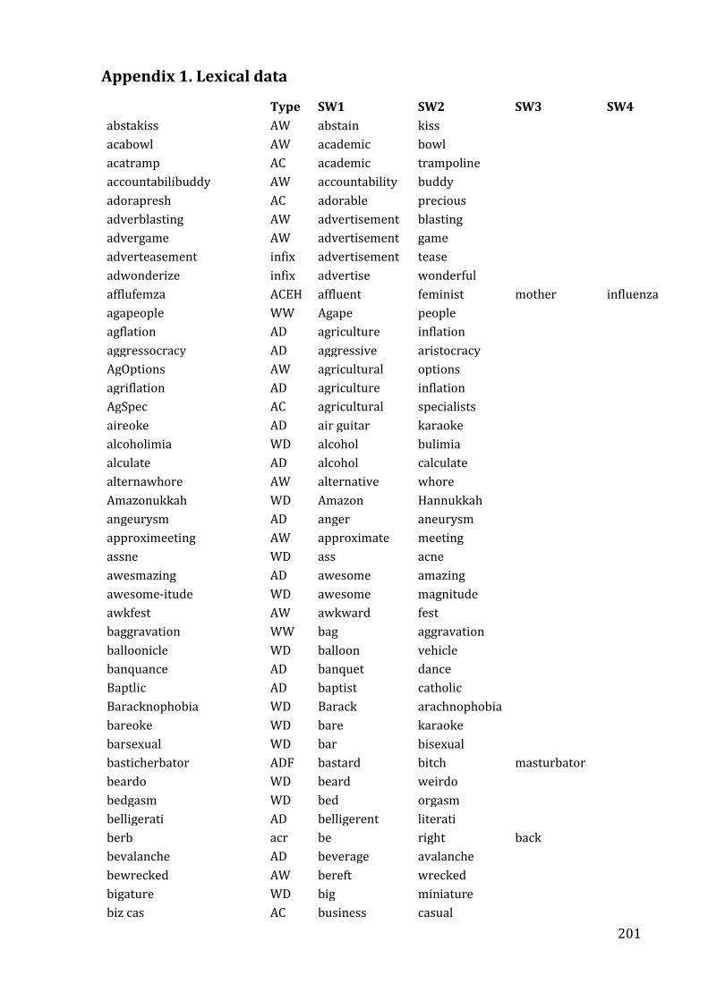
201

Appendix 1. Lexical data

Type SW1 SW2 SW3 SW4

abstakiss AW abstain kiss acabowl AW academic bowl acatramp AC academic trampoline accountabilibuddy AW accountability buddy adorapresh AC adorable precious adverblasting AW advertisement blasting advergame AW advertisement game adverteasement infix advertisement tease adwonderize infix advertise wonderful afflufemza ACEH affluent feminist mother influenza

agapeople WW Agape people agflation AD agriculture inflation aggressocracy AD aggressive aristocracy AgOptions AW agricultural options agriflation AD agriculture inflation AgSpec AC agricultural specialists aireoke AD air guitar karaoke alcoholimia WD alcohol bulimia alculate AD alcohol calculate alternawhore AW alternative whore Amazonukkah WD Amazon Hannukkah angeurysm AD anger aneurysm approximeeting AW approximate meeting assne WD ass acne awesmazing AD awesome amazing awesome-itude WD awesome magnitude awkfest AW awkward fest baggravation WW bag aggravation balloonicle WD balloon vehicle banquance AD banquet dance Baptlic AD baptist catholic Baracknophobia WD Barack arachnophobia bareoke WD bare karaoke barsexual WD bar bisexual basticherbator ADF bastard bitch masturbator

beardo WD beard weirdo bedgasm WD bed orgasm belligerati AD belligerent literati berb acr be right back

bevalanche AD beverage avalanche bewrecked AW bereft wrecked bigature WD big miniature biz cas AC business casual

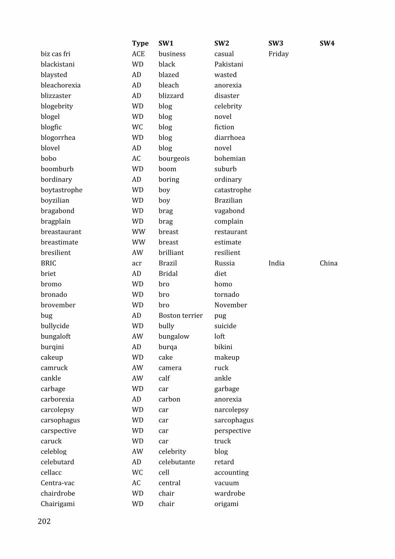
202


biz cas fri ACE business casual Friday blackistani WD black Pakistani

blaysted AD blazed wasted bleachorexia AD bleach anorexia blizzaster AD blizzard disaster blogebrity WD blog celebrity blogel WD blog novel blogfic WC blog fiction blogorrhea WD blog diarrhoea blovel AD blog novel bobo AC bourgeois bohemian boomburb WD boom suburb bordinary AD boring ordinary boytastrophe WD boy catastrophe boyzilian WD boy Brazilian bragabond WD brag vagabond bragplain WD brag complain breastaurant WW breast restaurant breastimate WW breast estimate bresilient AW brilliant resilient BRIC acr Brazil Russia India China

briet AD Bridal diet bromo WD bro homo bronado WD bro tornado brovember WD bro November bug AD Boston terrier pug bullycide WD bully suicide bungaloft AW bungalow loft burqini AD burqa bikini cakeup WD cake makeup camruck AW camera ruck cankle AW calf ankle carbage WD car garbage carborexia AD carbon anorexia carcolepsy WD car narcolepsy carsophagus WD car sarcophagus carspective WD car perspective caruck WD car truck celeblog AW celebrity blog celebutard AD celebutante retard cellacc WC cell accounting Centra-vac AC central vacuum chairdrobe WD chair wardrobe Chairigami WD chair origami

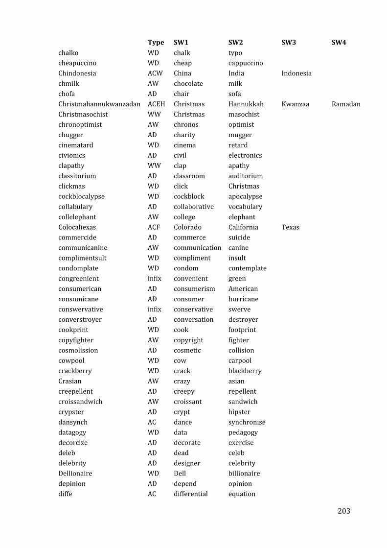
203


chalko WD chalk typo cheapuccino WD cheap cappuccino Chindonesia ACW China India Indonesia

chmilk AW chocolate milk chofa AD chair sofa Christmahannukwanzadan ACEH Christmas Hannukkah Kwanzaa Ramadan

Christmasochist WW Christmas masochist chronoptimist AW chronos optimist chugger AD charity mugger cinematard WD cinema retard civionics AD civil electronics clapathy WW clap apathy classitorium AD classroom auditorium clickmas WD click Christmas cockblocalypse WD cockblock apocalypse collabulary AD collaborative vocabulary collelephant AW college elephant Colocaliexas ACF Colorado California Texas

commercide AD commerce suicide communicanine AW communication canine complimentsult WD compliment insult condomplate WD condom contemplate congreenient infix convenient green consumerican AD consumerism American consumicane AD consumer hurricane conswervative infix conservative swerve converstroyer AD conversation destroyer cookprint WD cook footprint copyfighter AW copyright fighter cosmolission AD cosmetic collision cowpool WD cow carpool crackberry WD crack blackberry Crasian AW crazy asian creepellent AD creepy repellent croissandwich AW croissant sandwich crypster AD crypt hipster dansynch AC dance synchronise datagogy WD data pedagogy decorcize AD decorate exercise deleb AD dead celeb delebrity AD designer celebrity Dellionaire WD Dell billionaire depinion AD depend opinion diffe AC differential equation

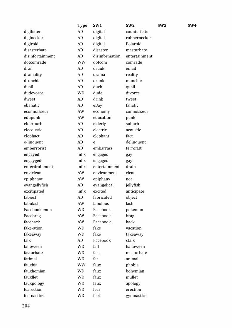
204


digifeiter AD digital counterfeiter diginecker AD digital rubbernecker digiroid AD digital Polaroid disasterbate AD disaster masturbate disinfortainment AD disinformation entertainment dotcomrade WW dotcom comrade drail AD drunk email dramality AD drama reality drunchie AD drunk munchie duail AD duck quail dudevorce WD dude divorce dweet AD drink tweet ebanatic AD eBay fanatic econnoisseur AW economy connoisseur edupunk AW education punk elderburb AD elderly suburb elecoustic AD electric acoustic elephact AD elephant fact e-linquent AD e delinquent emberrorist AD embarrass terrorist engayed infix engaged gay engayged infix engaged gay enterdrainment infix entertainment drain enviclean AW environment clean epiphanot AW epiphany not evangellyfish AD evangelical jellyfish excitipated infix excited anticipate fabject AD fabricated object fabulash AW fabulous lash Facebookemon WD Facebook pokemon Facebrag AW Facebook brag facehack AW Facebook hack fake-ation WD fake vacation fakeaway WD fake takeaway falk AD Facebook stalk falloween WD fall halloween fasturbate WD fast masturbate fatimal WD fat animal fauxbia WW faux phobia fauxhemian WD faux bohemian fauxllet WD faux mullet fauxpology WD faux apology fearection WD fear erection feetnastics WD feet gymnastics

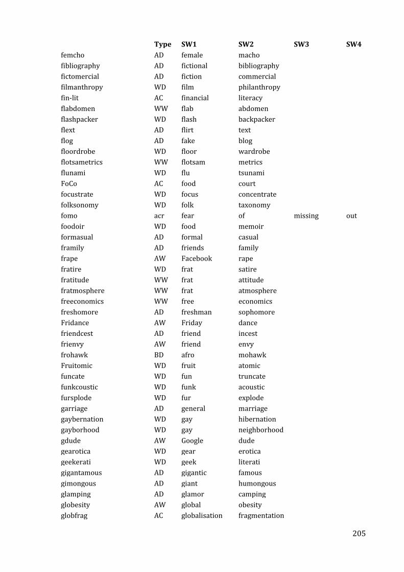
205


femcho AD female macho fibliography AD fictional bibliography fictomercial AD fiction commercial filmanthropy WD film philanthropy fin-lit AC financial literacy flabdomen WW flab abdomen flashpacker WD flash backpacker flext AD flirt text flog AD fake blog floordrobe WD floor wardrobe flotsametrics WW flotsam metrics flunami WD flu tsunami FoCo AC food court focustrate WD focus concentrate folksonomy WD folk taxonomy fomo acr fear of missing out

foodoir WD food memoir formasual AD formal casual framily AD friends family frape AW Facebook rape fratire WD frat satire fratitude WW frat attitude fratmosphere WW frat atmosphere freeconomics WW free economics freshomore AD freshman sophomore Fridance AW Friday dance friendcest AD friend incest frienvy AW friend envy frohawk BD afro mohawk Fruitomic WD fruit atomic funcate WD fun truncate funkcoustic WD funk acoustic fursplode WD fur explode garriage AD general marriage gaybernation WD gay hibernation gayborhood WD gay neighborhood gdude AW Google dude gearotica WD gear erotica geekerati WD geek literati gigantamous AD gigantic famous gimongous AD giant humongous glamping AD glamor camping globesity AW global obesity globfrag AC globalisation fragmentation

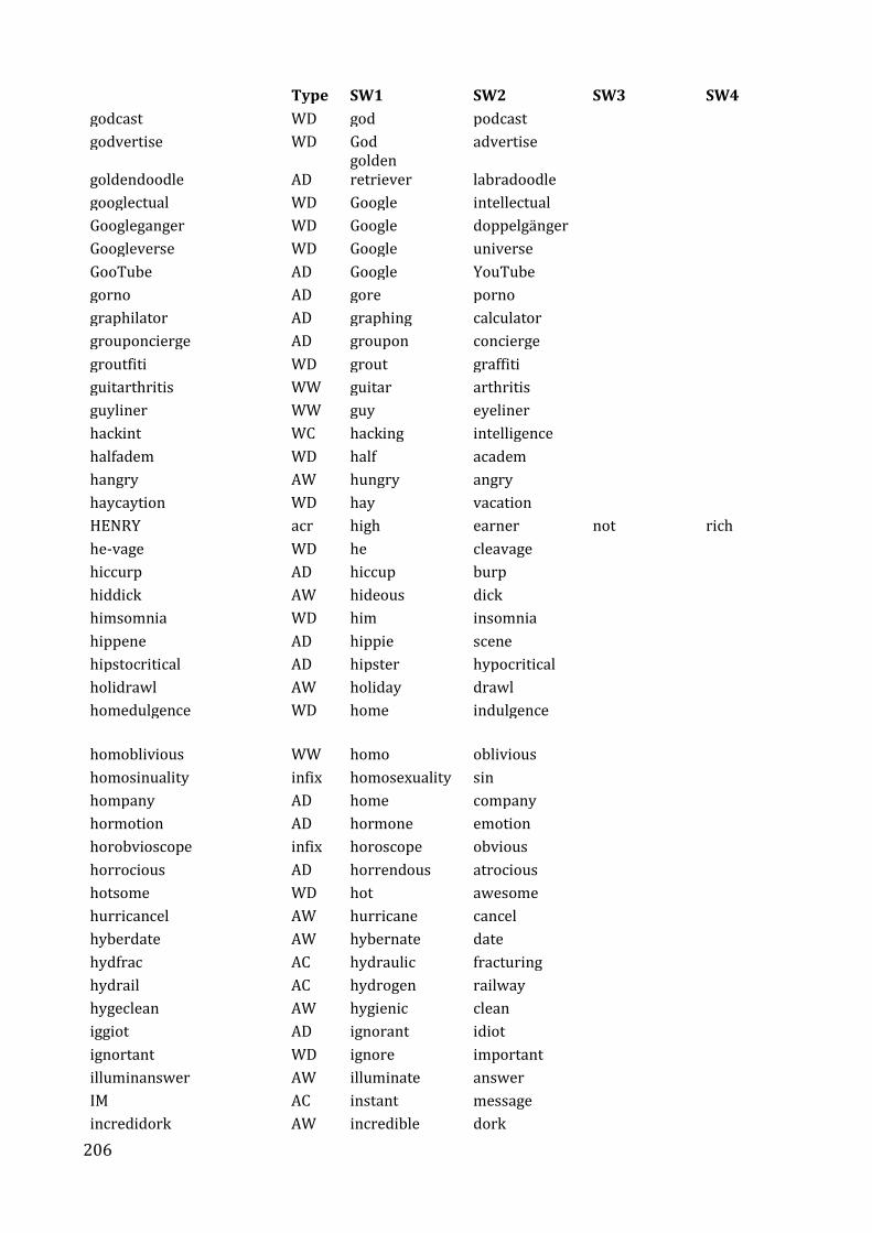
206


godcast WD god podcast godvertise WD God advertise

goldendoodle AD golden retriever labradoodle

googlectual WD Google intellectual Googleganger WD Google doppelgänger Googleverse WD Google universe GooTube AD Google YouTube gorno AD gore porno graphilator AD graphing calculator grouponcierge AD groupon concierge groutfiti WD grout graffiti guitarthritis WW guitar arthritis guyliner WW guy eyeliner hackint WC hacking intelligence halfadem WD half academ hangry AW hungry angry haycaytion WD hay vacation HENRY acr high earner not rich

he-vage WD he cleavage hiccurp AD hiccup burp hiddick AW hideous dick himsomnia WD him insomnia hippene AD hippie scene hipstocritical AD hipster hypocritical holidrawl AW holiday drawl homedulgence WD home indulgence

homoblivious WW homo oblivious homosinuality infix homosexuality sin hompany AD home company hormotion AD hormone emotion horobvioscope infix horoscope obvious horrocious AD horrendous atrocious hotsome WD hot awesome hurricancel AW hurricane cancel hyberdate AW hybernate date hydfrac AC hydraulic fracturing hydrail AC hydrogen railway hygeclean AW hygienic clean iggiot AD ignorant idiot ignortant WD ignore important illuminanswer AW illuminate answer IM AC instant message incredidork AW incredible dork

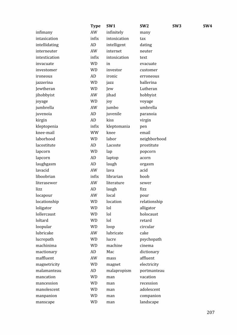
207


infimany AW infinitely many intaxication infix intoxication tax intellidating AD intelligent dating interneuter AW internet neuter intextication infix intoxication text invacuate WD in evacuate investomer WD investor customer ironeous AD ironic erroneous jazzerina WD jazz ballerina Jewtheran WD Jew Lutheran jihobbyist AW jihad hobbyist joyage WD joy voyage jumbrella AW jumbo umbrella juvenoia AD juvenile paranoia kirgin AD kiss virgin kleptopenia infix kleptomania pen knee-mail WW knee email laborhood WD labor neighborhood lacostitute AD Lacoste prostitute lapcorn WD lap popcorn lapcorn AD laptop acorn laughgasm AD laugh orgasm lavacid AW lava acid liboobrian infix librarian boob literasewer AW literature sewer lizz AD laugh fizz locapour AW local pour locationship WD location relationship loligator WD lol alligator lollercaust WD lol holocaust loltard WD lol retard loopular WD loop circular lubricake AW lubricate cake lucrepath WD lucre psychopath machinima WD machine cinema mactionary AD Mac dictionary maffluent AW mass affluent magnetricity WD magnet electricity malamanteau AD malapropism portmanteau mancation WD man vacation mancession WD man recession manolescent WD man adolescent manpanion WD man companion manscape WD man landscape

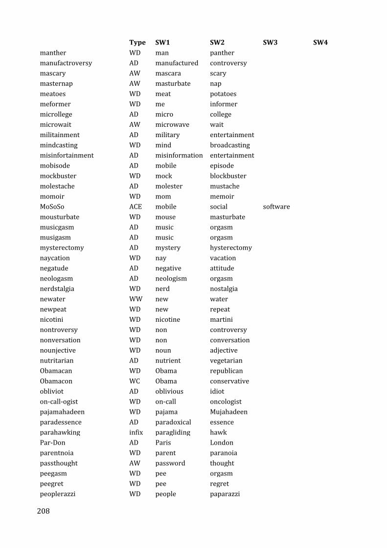
208


manther WD man panther manufactroversy AD manufactured controversy mascary AW mascara scary masternap AW masturbate nap meatoes WD meat potatoes meformer WD me informer microllege AD micro college microwait AW microwave wait militainment AD military entertainment mindcasting WD mind broadcasting misinfortainment AD misinformation entertainment mobisode AD mobile episode mockbuster WD mock blockbuster molestache AD molester mustache momoir WD mom memoir MoSoSo ACE mobile social software

mousturbate WD mouse masturbate musicgasm AD music orgasm musigasm AD music orgasm mysterectomy AD mystery hysterectomy naycation WD nay vacation negatude AD negative attitude neologasm AD neologism orgasm nerdstalgia WD nerd nostalgia newater WW new water newpeat WD new repeat nicotini WD nicotine martini nontroversy WD non controversy nonversation WD non conversation nounjective WD noun adjective nutritarian AD nutrient vegetarian Obamacan WD Obama republican Obamacon WC Obama conservative obliviot AD oblivious idiot on-call-ogist WD on-call oncologist pajamahadeen WD pajama Mujahadeen paradessence AD paradoxical essence parahawking infix paragliding hawk Par-Don AD Paris London parentnoia WD parent paranoia passthought AW password thought peegasm WD pee orgasm peegret WD pee regret peoplerazzi WD people paparazzi

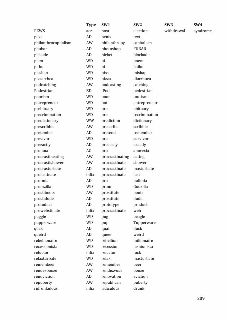
209


PEWS acr post election withdrawal syndrome

pext AD penis text philanthrocapitalism AW philanthropy capitalism phobar AD photoshop FUBAR pickade AD picket blockade piem WD pi poem pi-ku WD pi haiku pisshap WD piss mishap pizzarrhea WD pizza diarrhoea podcatching AW podcasting catching Podestrian BD iPod pedestrian poorism WD poor tourism potrepreneur WD pot entrepreneur prebituary WD pre obituary precrimination WD pre recrimination predictionary WW prediction dictionary prescribble AW prescribe scribble pretember AD pretend remember previvor WD pre survivor prezactly AD precisely exactly pro-ana AC pro anorexia procrastineating AW procrastinating eating procrastishower AW procrastinate shower procrasturbate AD procrastinate masturbate profastinate infix procrastinate fast pro-mia AD pro bulimia promzilla WD prom Godzilla prostiboots AW prostitute boots prostidude AD prostitute dude protoduct AD prototype product prowebstinate infix procrastinate web puggle WD pug beagle pupperware WD pup Tupperware quck AD quail duck queird AD queer weird rebellionaire WD rebellion millionaire recessionista WD recession fashionista refuctor infix refactor fuck relaxturbate WD relax masturbate remembeer AW remember beer rendezbooze AW rendezvous booze renoviction AD renovation eviction repuberty AW republican puberty ridrunkulous infix ridiculous drunk

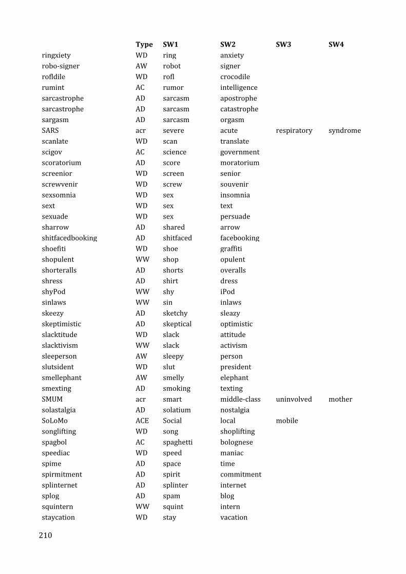
210


ringxiety WD ring anxiety robo-signer AW robot signer rofldile WD rofl crocodile rumint AC rumor intelligence sarcastrophe AD sarcasm apostrophe sarcastrophe AD sarcasm catastrophe sargasm AD sarcasm orgasm SARS acr severe acute respiratory syndrome

scanlate WD scan translate scigov AC science government scoratorium AD score moratorium screenior WD screen senior screwvenir WD screw souvenir sexsomnia WD sex insomnia sext WD sex text sexuade WD sex persuade sharrow AD shared arrow shitfacedbooking AD shitfaced facebooking shoefiti WD shoe graffiti shopulent WW shop opulent shorteralls AD shorts overalls shress AD shirt dress shyPod WW shy iPod sinlaws WW sin inlaws skeezy AD sketchy sleazy skeptimistic AD skeptical optimistic slacktitude WD slack attitude slacktivism WW slack activism sleeperson AW sleepy person slutsident WD slut president smellephant AW smelly elephant smexting AD smoking texting SMUM acr smart middle-class uninvolved mother

solastalgia AD solatium nostalgia SoLoMo ACE Social local mobile

songlifting WD song shoplifting spagbol AC spaghetti bolognese speediac WD speed maniac spime AD space time spirmitment AD spirit commitment splinternet AD splinter internet splog AD spam blog squintern WW squint intern staycation WD stay vacation

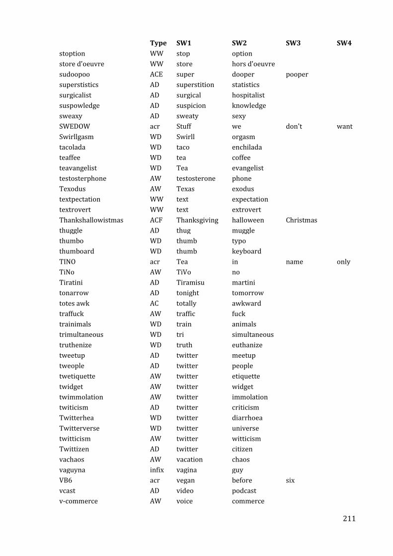
211


stoption WW stop option store d'oeuvre WW store hors d'oeuvre sudoopoo ACE super dooper pooper

superstistics AD superstition statistics surgicalist AD surgical hospitalist suspowledge AD suspicion knowledge sweaxy AD sweaty sexy SWEDOW acr Stuff we don't want

Swirllgasm WD Swirll orgasm tacolada WD taco enchilada teaffee WD tea coffee teavangelist WD Tea evangelist testosterphone AW testosterone phone Texodus AW Texas exodus textpectation WW text expectation textrovert WW text extrovert Thankshallowistmas ACF Thanksgiving halloween Christmas

thuggle AD thug muggle thumbo WD thumb typo thumboard WD thumb keyboard TINO acr Tea in name only

TiNo AW TiVo no Tiratini AD Tiramisu martini tonarrow AD tonight tomorrow totes awk AC totally awkward traffuck AW traffic fuck trainimals WD train animals trimultaneous WD tri simultaneous truthenize WD truth euthanize tweetup AD twitter meetup tweople AD twitter people twetiquette AW twitter etiquette twidget AW twitter widget twimmolation AW twitter immolation twiticism AD twitter criticism Twitterhea WD twitter diarrhoea Twitterverse WD twitter universe twitticism AW twitter witticism Twittizen AD twitter citizen vachaos AW vacation chaos vaguyna infix vagina guy VB6 acr vegan before six

vcast AD video podcast v-commerce AW voice commerce

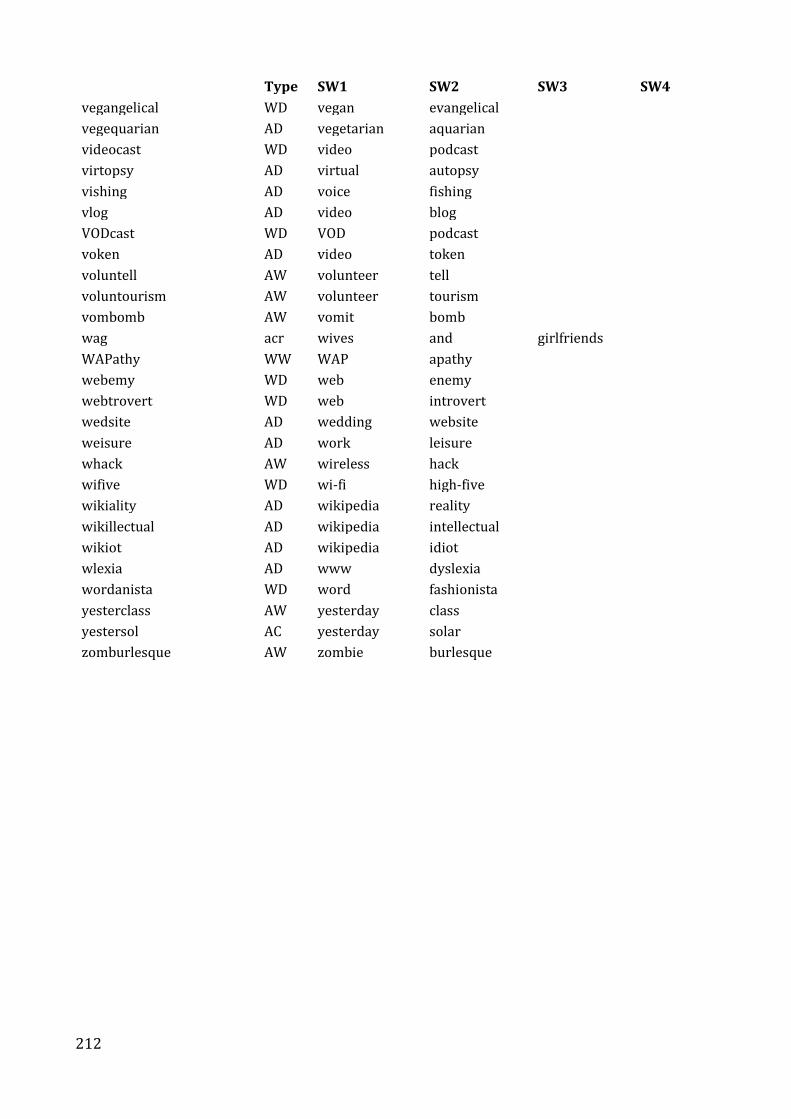
212


vegangelical WD vegan evangelical vegequarian AD vegetarian aquarian videocast WD video podcast virtopsy AD virtual autopsy vishing AD voice fishing vlog AD video blog VODcast WD VOD podcast voken AD video token voluntell AW volunteer tell voluntourism AW volunteer tourism vombomb AW vomit bomb wag acr wives and girlfriends

WAPathy WW WAP apathy webemy WD web enemy webtrovert WD web introvert wedsite AD wedding website weisure AD work leisure whack AW wireless hack wifive WD wi-fi high-five wikiality AD wikipedia reality wikillectual AD wikipedia intellectual wikiot AD wikipedia idiot wlexia AD www dyslexia wordanista WD word fashionista yesterclass AW yesterday class yestersol AC yesterday solar zomburlesque AW zombie burlesque

213

Appendix 2. Ethics Approval

214

215

Appendix 3. Information sheet for participants of the web-based

survey

School of Linguistics and Applied Language Studies

PO Box 600, Wellington 6140

tel: 4635600

fax: 4635604

Researcher: Natalia Beliaeva: [email protected]

Supervisors: Laurie Bauer: [email protected]

Paul Warren: [email protected]

Let’s have a word about words!

I am a PhD student in Linguistics at Victoria University of Wellington undertaking a research

project that will lead to a thesis. With this project, I am looking at how people use language

and understand new words.

This project has been granted ethical approval by the Victoria University of Wellington

Human Ethics Committee.

I am inviting native speakers of English to complete an online questionnaire which will take

around 15 minutes. In acknowledgement of your time and effort we will include you in the

prize draw for a gift voucher worth 100 NZ dollars.

By following the link below you give your consent for me to use your responses in the

research project.

The survey is strictly anonymous. Any personal information, e.g. age or first language, will be

collected for statistical reasons only and no identities will be associated with any responses.

The collected data will be stored in password protected file for the duration of this study.

The thesis will be submitted for marking to Victoria University of Wellington and deposited

in the University Library, after which it will become available electronically. I also intend to

publish articles based on the data in scholarly journals. Additionally, I will produce a

summary report of the findings of the project for participants which will be sent to you if you

make this request by ticking the appropriate box on the survey webpage. The collected data

will be destroyed 2 years after the conclusion of the research.

If you have any questions or would like to receive further information about the project, feel

free to contact me or my supervisors using the details provided above.

To start the survey, follow this link: http://vuw.qualtrics.com/SE/?SID=SV_bBJRbTNWX8CTMod

mailto:[email protected]



http://vuw.qualtrics.com/SE/?SID=SV_bBJRbTNWX8CTMod

216

217

Appendix 4. Survey stimuli

Main survey

The questions in Part 1 were presented to the participants in a random order, preceded by the instruction that is given below. Each question contained only one of the four definitions of the word in bold type. Part 2 questions and were presented after Part 1, in the same order as in this sample. Part 1 Thank you for agreeing to participate in our survey. It should take around 15 minutes to answer all the questions. You will see a total of 64 sentences displayed successively on 10 pages. After each sentence there is a definition for the word in bold type. Please read the sentences and answer how successfully you think each definition explains the word by choosing the appropriate option.

1. In fact, Ontario may have some catching up to do if it's serious about being a world leader in hydrails. A European consortium called The Hydrogen Train concluded a study last year that looked at what it would take to demonstrate a hydrogen train in Denmark by 2010.

hydrail – 1) hydrogen railway 2) trains that use hydrogen fuel 3) a railway system that uses highly flammable gas fuel 4) trains that use highly flammable gas fuel

2. I am a scigov double major.

scigov – 1) science and government studies 2) science and politics studies 3) natural and government studies 4) natural and politics studies

3. Bobos talk like hippies but walk like yuppies, decrying materialism while

indulging in all manner of luxuries. bobo –

1) a bourgeois bohemian 2) a socially unconventional bourgeois person 3) a person who likes both a bohemian and a luxurious lifestyle 4) a socially unconventional person who likes a luxurious lifestyle

4. For 18 year Consolidated Credit Counseling Services focused on educating youth

about money management and finlit topics. finlit –

1) financial literacy 2) the ability to understand financial texts 3) literacy in the field of money and economics 4) the ability to understand texts related to money and economics

218

5. He says, and others back him up, that the Pentagon took dubious accounts from émigrés close to Ibrahim Zuhair and gave these tales credibility they did not deserve. Intelligence analysts ... refer contemptuously to recent work as “rumint”...

rumint – 1) rumour intelligence 2) sophisticated information based on rumours rather than facts 3) intelligence information from unreliable sources 4) sophisticated information from unreliable sources

6. You only need to look into a person's bedroom to realize the seriousness of

globfrag. He is stuck on his computer 24/7 with instant knowledge from all over the globe at his fingertips, yet does not know what his family is up to.

globfrag – 1) globalisation and simultaneous fragmentation 2) globalisation and simultaneous breakdown in connections between people 3) international integration and simultaneous fragmentation 4) international integration and simultaneous breakdown in connections between

people

7. Someone lounges lazily on the Acatramp, ... diligent studiers read on chairs outside as the stacks blare, groups cluster on the fourth floor balcony, and a Frisbee whizzes past my ear: it’s Friday afternoon.

acatramp – 1) an academic trampoline 2) an academic bouncing device 3) a trampoline for students and professors 4) a bouncing device for students and professors

8. "Oh my goodness, Michael gave me the most beautiful bouquet for our six-month

anniversary today.” – “Aww, that’s adorapresh!” adorapresh –

1) adorable and precious 2) adorable and valuable 3) enchanting and precious 4) enchanting and valuable

9. Whip out your best biz cas for this event.

biz cas – 1) business casual clothing 2) business informal clothing 3) workplace casual clothing 4) workplace informal clothing

10. IM me later

IM – 1) instant message 2) instant communication 3) real-time online message 4) real-time online communication

219

11. When she heard music coming over the grocery store's PA system, Amie started

to dansynch until the music was over. dansynch –

1) dance in synchronization with the music 2) dance in time with the music 3) move rhythmically in synchronization with the music 4) move rhythmically in time with the music

12. Diffe is the hardest and perhaps most widely taken math class at our university.

diffe – 1) differential equations 2) mathematical statements involving differentials 3) equations involving derivatives of functions 4) mathematical statements involving derivatives of functions

13. Do you want to eat at the FoCo tonight?

FoCo – 1) a food court 2) an area with food outlets 3) a snack bar and restaurant court 4) an area with snack bars and restaurants

14. With the rushed passage into law of the Digital Economy Act this month, the fight

over copyright enters a new phase. Previous to this, most copyfighters operated under the rubric that a negotiated peace was possible between the thrashing entertainment giants and civil society.

copyfighter – 1) a copyright fighter 2) a person who protests against copyright 3) a person who fights against legal control over created work 4) a person who protests against legal control over created work

15. The journalistic celeblog has its roots in fertile soil — the hallowed tradition of

"Nobody asked me, but..." columns that newspaper hacks have for decades used to fill space with short-paragraph rambles on the folly of Liberals, the folly of Conservatives, or the folly of the guy who invented the shrink wrap on compact disks.

celeblog – 1) a blog written by or about a celebrity 2) a web journal written by or about a celebrity 3) a blog written by or about a famous person 4) a web journal written by or about a famous person

16. A growing number of tourists – especially aging Baby Boomers and students – are

keen to explore some of the darkest corners of the world, and maybe even work there for a while on “voluntourism” projects.

voluntourism – 1) volunteer tourism 2) volunteering while travelling 3) tourism that involves doing unpaid work

220

4) doing unpaid work while travelling

17. But this kind of flexibility – we call it approximeeting – can also engender a new sense of insecurity.

approximeeting – 1) an approximate meeting arrangement 2) an approximate appointment arrangement 3) a meeting arrangement with no precise details specified 4) an appointment arrangement with no precise details specified

18. While people may be tricked into giving up their passwords, smartcards may be

lost or stolen, as can biometric templates stored on computers for comparing eye or fingerprint scans, so-called “passthoughts” are unique.

passthought – 1) a thought pattern used as a password 2) a brain signal used as a password 3) a thought pattern giving access to a computer system 4) a brain signal giving access to a computer system

19. Most of these will be redevelopments into what some people call "bungalofts" —

houses bought for about $180,000 by young professionals and modernized ... with clear sight lines to the backyard and custom millwork.

bungaloft – 1) a bungalow with a loft 2) a bungalow with an attic 3) a detached low-rise house with a loft 4) a detached low-rise house with an attic

20. Officials say advergames promote repeat traffic to Web sites and reinforce

brands in compelling ways. Because users choose to register to be eligible for prizes, the games help marketers collect customer data.

advergames – 1) games that incorporate advertisement 2) entertainment programmes that incorporate advertisement 3) games that incorporate commercial announcements 4) entertainment programmes that incorporate commercial announcements

21. Where is that steak I ordered? We've been waiting for an hour and a half here. The service here is terrible! I'm starving! I don't know about you, but I'm starting to feel really hangry!

hangry – 1) hungry and angry 2) hungry and strongly displeased 3) feeling need for food and angry 4) feeling need for food and strongly displeased

22. Hey, did you see Jane's newest Facebrag? Eesh.

Facebrag – 1) Facebook bragging 2) Facebook boasting

221

3) bragging in a social network 4) boasting in a social network

23. Crammer News uses the opinions of politiclones to bolster support for the

President’s Administration. politiclones –

1) people who clone their political opinions from others 2) people who copy their political opinions from others 3) people who clone their opinions about governmental actions from others 4) people who copy their opinions about governmental actions from others

24. Jackie was filled with frienvy as she walked through the halls with her best

friend Tracey, because all of the guys were complimenting Tracey on her hot new look.

frienvy – 1) envy of a friend 2) desire for something that a friend might have 3) envy of a close acquaintance 4) desire for something that a close acquaintance might have

25. Try eating our new Croissandwich!

croissandwich – 1) the hybrid of croissant and sandwich 2) a croissant which is sliced and filled 3) a sandwich made of a crescent shaped bread roll 4) a sliced and filled crescent shaped bread roll

26. Classes are hurricancelled!

hurricancelled – 1) cancelled because of a hurricane 2) called off because of a hurricane 3) cancelled because of a severe storm 4) called off because of a severe storm

27. The Twitter-based application, twhirl, is an example of a handy twidget.

twidget – 1) a Twitter widget 2) a small software application for Twitter 3) a widget for a microblogging service 4) a small software application for a microblogging service

28. Call it the courtship equivalent to the slow-food movement. Call it a backlash

against point and click matchmaking. Whichever, intellidating – an unhurried, decidedly highbrow approach to mating – is catching on in Boston, New York, Toronto and beyond…

intellidating – 1) dating that emphasizes intelligence 2) romantic relationships that emphasize intelligence 3) dating that involves mentally stimulating activity 4) romantic relationships that involve mentally stimulating activity

222

29. “Investomers”, or people who both hold stock in a particular company and buy products from that company, are generally more loyal and more profitable than their nonequity-owning counterparts.

investomer – 1) a customer who is also an investor 2) a client who is also an investor 3) a customer who is also a shareholder 4) a client who is also a shareholder

30. So, after a year of trying to figure out what I was going to do, I decided to quit my

ballet life and become a "Jazzerina!" jazzerina –

1) a ballerina who performs a jazz dance 2) a classical dancer who performs a jazz dance 3) a ballerina who performs an improvisation dance to syncopated music 4) a classical dancer who performs an improvisation dance to syncopated music

31. “Those pants don‘t make your butt look so big” – that’s a complimentsult!

complimentsult – 1) a compliment which is also an insult 2) a compliment which is also offensive 3) praise which is also an insult 4) praise which is also offensive

32. The move to "homedulgence" is one way consumers can ride out the recession

and it is predicted it will soon extend to many other areas of life, such as mix-your-own cocktails evenings and home dining clubs.

homedulgence – 1) home-based indulgence 2) home-based entertainment 3) indulgence without going out 4) entertainment without going out

33. Shoppers trying to survive the credit crunch are also spending less on takeaways

and making home-made "fakeaways" of their favourite dishes. fakeaway –

1) a fake takeaway 2) a fake restaurant meal 3) a homemade meal similar to takeaway 4) a homemade meal similar to one made in a restaurant

34. Uh, you might want to get rid of all this carbage before you pick up your date

tonight. carbage –

1) garbage in one’s car 2) trash in one’s car 3) garbage in one’s vehicle 4) trash in one’s vehicle

35. The deluded women who bought Boyzilians as gifts for their boyfriends need a

reality check.

223

boyzilian – 1) Brazilian waxing for boys 2) bikini waxing for boys 3) Brazilian waxing for men 4) bikini waxing for men

36. Look up around your city and what do you see? A bird? A plane? No, it's a pair of

mangy sneakers dangling from the powerlines. Shoe-flinging, or shoefiti, has emerged as one of the more inexplicable forms of cultural expression in inner-city Melbourne.

shoefiti – 1) graffiti made of shoes 2) street decoration made of shoes 3) graffiti made of footwear 4) street decoration made of footwear

37. "I want all viewers to feel a part of this mission." Some might liken this type of

documentary and fundraising event to the trend toward "filmanthrophy." filmanthropy –

1) making films for philanthropic reasons 2) making films to raise money for charity 3) moviemaking for philanthropic reasons 4) moviemaking to raise money for charity

38. Many of us will be familiar with the basest form of ringxiety — when one phone

rings and everyone in the vicinity suddenly starts checking their pockets or handbags with frantic abandon.

ringxiety – 1) anxiety caused by telephone ringing 2) uneasiness caused by telephone ringing 3) anxiety caused by the sound of a telephone call 4) uneasiness caused by the sound of a telephone call

39. Just as we continue to educate fans about the right ways to enjoy music online,

we will continue to enforce our rights through the legal system. Songlifting is not without consequences.

songlifting – 1) online shoplifting of songs 2) unauthorised downloading of songs 3) online shoplifting of musical copyright material 4) unauthorised downloading of musical copyright material

40. Of the 68 miniature sets and models in The Lord Of The Rings, about 30 were

dubbed "bigatures" because they were so large and detailed, people could have actually lived in them.

bigature – 1) a big miniature 2) a big, rather than small, replica or model 3) a large scale model rather than miniature 4) a large scale, rather than small, replica or model

224

41. “Man, she was on Facebook flirting with everyone and talking about all her wild parties, but when we met in person she just stared at the floor and mumbled everytime I asked her something.” – “Yeah, sounds like she's kind of a webtrovert. “

webtrovert – 1) a web extrovert 2) a person who is socially confident and outgoing on the web 3) an internet extrovert 4) a person who is socially confident and outgoing on the internet

42. Tagging often produces strange, overlapping characterizations with surprisingly

beneficial results. Some have called the results a "folksonomy." folksonomy –

1) a folk taxonomy 2) a folk classification 3) a taxonomy based on people’s opinions 4) a classification based on people’s opinions

43. This is where I work with other people to scanlate manga. You're welcome to

help, no commitment needed. scanlate –

1) scan and translate 2) scan and convert into another language 3) convert into digital form and translate 4) convert into digital form and into another language

44. Magazines have taken to publishing before and after shots of "painfully thin

Kate", calling her "Queen of diets" and "Slimline Kate", and speculating on the "briet".

briet – 1) a diet for brides 2) a special course of food for brides 3) a diet for women just before marriage 4) a special course of food for women just before marriage

45. Is ‘sceptimistic’ the ideal mindset for a strategist?

sceptimistic – 1) both sceptical and optimistic 2) both sceptical and confident about the future 3) both doubting and optimistic 4) both doubting and confident about the future

46. Whether you are weathering the storm by building snowmen or plowing through

piles of snow on your driveway, we are asking for photos of how you honor Old Man Winter. And if you want to stay in the comfort of your home, just post a photo of your backyard blizzaster.

blizzaster – 1) a disaster caused by a blizzard 2) a sudden accident caused by a blizzard 3) a disaster caused by a snow storm 4) a sudden accident caused by a snow storm

225

47. 'Products blessed with paradessence somehow combine two mutually exclusive

states and satisfy both simultaneously. Ice cream melds eroticism and innocence. Air travel offers sanitised adventure. Amusement parks provide terror and reassurance. Automobiles render drivers reckless and safe.

paradessence – 1) a paradoxical essence 2) a paradoxical characteristic 3) a self-contradictory essence 4) a self-contradictory characteristic

48. Weisure has been fuelled by social networking sites like Facebook and MySpace,

where “friends” may actually be business partners or work colleagues. weisure –

1) a combination of work and leisure 2) a combination of business-related tasks and leisure 3) a combination of work and free time 4) a combination of business-related tasks and free time

49. While the IFA is protesting — and not "pickading" any of the plants — farmers

will not deliver animals across those protest lines. While some factories have their own supplies, these are estimated to be less than a fortnight's kill. With relations between the two sides deteriorating, "pickades" could well be the next step.

pickade – 1) a picket which is also a blockade 2) a picket which prevents goods or people from entering or leaving a place 3) people gathering outside a building to protest and to make a blockade 4) people gathering at a place to protest and to prevent goods or people from

entering or leaving it

50. I am promoting a new protoduct on this website. protoduct –

1) a prototype which is also a product 2) a prototype which is also released for sale 3) a preliminary version of something which is also a product 4) a preliminary version of something which is also released for sale

51. Once out, the tenants are not allowed to renew their leases until they agree to

monstrous rent increases, sometimes double what they paid before the renoviction.

renoviction – 1) renovation of an apartment coupled with the eviction of its tenants 2) renovation of an apartment coupled with the expulsion of its tenants 3) repair works in an apartment coupled with the eviction of its tenants 4) repair works in an apartment coupled with the expulsion of its tenants

52. If I want to share my word tags with a community, I’m contributing to a

collabulary. collabulary –

226

1) collaboratively compiled vocabulary 2) collaboratively compiled body of words 3) a vocabulary compiled by several parties working together 4) a body of words compiled by several parties working together

53. Last year chuggers coaxed 700,000 donors into pledging $240 million to

charities over the next five years. About 100 charities hire chuggers to boost revenues. Although one high-street fundraiser can cost as much as $100 a day, charities say they are good value.

chugger – 1) a charity mugger 2) a person who forces people to donate money for charity 3) a fundraising mugger 4) a person who forces people to donate money for fundraising

54. "No one's allowed in the living room — only adults," says Zalta, flopping down on

his favourite piece of furniture, the "chofa". chofa –

1) a hybrid of a chair and a sofa 2) a wide and soft chair 3) a small sofa for one person 4) a wide and soft seat for one person

55. "Dramalities," they say, are satiating people's needs for sanitized gossip, Peeping

Tomism, and the pathetic desire to feel superior. dramality –

1) a combination of drama and reality 2) a combination of drama and real-life events 3) a combination of role play and reality 4) a combination of role play and real-life events

56. Where once there were objects, now there are well, fabjects.

fabject – 1) a fabricated object 2) a fabricated thing 3) an object invented in order to deceive 4) a thing invented in order to deceive

57. Lenny’s neighbours called the cops to complain about his late night guitar solos,

so now he has to go elecoustic. elecoustic –

1) an electric guitar used as an acoustic one 2) an electric guitar used unplugged 3) an amplified guitar used as an acoustic guitar 4) an amplified guitar used unplugged

58. Put down your phone and stop flexting.

flexting – 1) flirting while texting 2) flirting while sending SMS 3) demonstrating playfully amorous behaviour while texting

227

4) demonstrating playfully amorous behaviour while sending SMS 59. I really like this blogfic. I plan on continuing to read it until it's abandoned or the

writer brings it to a sensible conclusion. blogfic –

1) blog fiction 2) blog literature 3) web journal fiction 4) web journal literature

60. According to a US presidential commission, the global population with the

computer skills required for hackint operations and other forms of cyber-attack against important Western targets has grown from a few thousand 20 years ago to about 19 million today.

hackint – 1) hacking intelligence 2) obtaining secret information by hacking 3) unauthorised accessing a computer system to get intelligence 4) obtaining secret information unauthorised accessing a computer system

61. According to stock-tracking firm IPO.com, more than a quarter of the 71 netcos

that went public in the past year are now trading under their offering price. netco –

1) an internet company 2) an internet business 3) an online company 4) an online business

62. See the white earphones, she's got to be a podestrian.

podestrian – 1) a pedestrian with an iPod 2) a person walking on the street with an iPod 3) a pedestrian with a specific portable digital media player 4) a person walking on the street with a specific portable digital media player

63. Sporting a sharp 'frohawk’ that day, though, he was not exactly easy to picture in

a choir robe. frohawk –

1) an afro hairstyle shaped as a mohawk 2) an afro hairstyle in which both sides of the head are shaven 3) a hairstyle with frizzy hair shaped as a mohawk 4) a hairstyle with frizzy hair in which both sides of the head are shaven

64. The largest group of Obamacons hail from the libertarian wing of the movement.

Obamacon – 1) a Conservative who supports Obama 2) a person who does not support the Democratic party but supports Obama 3) a Conservative who supports the Democratic president 4) a person who does not support the Democratic party but supports the

Democratic president

228

Part 2 Please answer the following questions about yourself

1. Are you male or female? male_____; female_____

2. What is your age? 18-25_____; 26-30_____; 31-40_____; 41-50_____; 51-60_____; over 60_____;

3. What is your native language? English_____; other (please specify) ________________

4. Have you taken a university course in linguistics? Y____; N_____ .

5. Do you want to take part in the prize draw for a gift voucher worth 100 NZ dollars? Y_____; N_____; if yes, please provide your e-mail address: __________________________________________________

6. Do you want to receive an e-mail with a report of the research when it is completed? Y_____; N_____.

(the e-mail address will not be associated with your responses and will not be used for any purposes other than prize draw and sending a report of the research).

Additional survey stimuli (with WW target words)

65. Ebbesmeyer has found that rubber duckies and sneakers lost off container ships have a

way of capturing the public’s attention. He has used them over the past two decades to

illustrate the persistence of plastics and other floating trash in the oceans. Now, along with

science writer Eric Scigliano, he has written Flotsametrics and the Floating World: How One

Man’s Obsession with Runaway Sneakers and Rubber Ducks Revolutionized Ocean Science.

flotsametrics –

1) a system of metrics using flotsam

2) calculating something using flotsam

3) a system of metrics using wreckage or cargo floating on the sea

4) calculating something using wreckage or cargo floating on the sea

66. In general, you can't fight against your genetic strengths and come off the conqueror. If

you're the type of young adult that gets called "cute" and "sweet" over "hot," guyliner isn't

likely for you. Eye makeup doesn't tend to make "hot" out of "sweet," but it certainly can

make "yikes."

guyliner - 1) an eyeliner for guys

2) an eye makeup product for guys

3) an eyeliner for men

4) an eye makeup product for men

67. Predictionary is about blank spaces in language and culture and their formative role in

conceptual and artistic creativity.

predictionary - 1) a dictionary containing predictions

2) a reference book containing predictions

229

3) a dictionary containing statements about the future

4) a reference book containing statements about the future

68. Michael Robertson says teachers setting up Internet projects underestimate the pleasure

people get out of doing something that feels like a public service yet requires no more than a

few keystrokes. "It's all fed by slacktivism," he said, "the desire people have to do something

good without getting out of their chair."

slacktivism - 1) slack activism

2) slack efforts to promote or impede changes

3) lazy activism

4) lazy efforts to promote or impede changes

69. Ryan's uncomfortable laughter at the Secret Santa Pot Luck indicated he was a

Christmasochist.

Christmasochist - 1) a Christmas masochist

2) a person involved in Christmas activities despite suffering from them

3) a yuletide masochist

4) a person involved in yuletide activities despite suffering from them

70. Because Doug downloaded the new hit "Outrageous" he was totally shyPod when Dru

wanted to take a peek at his Library.

ShyPod - 1) feeling shy about sharing the contents of one's iPod

2) feeling shy about sharing the contents of one's portable media player

3) feeling bashful about sharing the contents of one's iPod

4) feeling bashful about sharing the contents of one's portable media player

71. "That graduation ceremony was so long, I got clapathy!"

clapathy - 1) apathy caused by excessive clapping

2) indifference caused by excessive clapping

3) apathy caused by excessive applauding

4) indifference caused by excessive applauding

72. Kelly: "So how'd the conversation go with Bill last night?"

Wendy: "Ah he's such a textrovert. We didn't make any progress until I went home and he

spilled his guts over texts."

textrovert - 1) a texting extrovert

2) a person who is socially outgoing while texting

3) an SMS extrovert

4) a person who is socially outgoing while sending SMS

73. “Man my wrists hurt from my guitarthritis”

guitarthritis -

230

1) arthritis caused by playing the guitar

2) inflammation of a joint caused by playing the guitar

3) arthritis caused by playing a musical instrument

4) inflammation of a joint caused by playing a musical instrument

74. “So who’s this NrdPowr32 guy?”

“I dunno. Just a dotcomrade of mine.”

dotcomrade - 1) a dotcom comrade

2) a dotcom friend

3) an internet comrade

4) an internet friend

75. “A marvellous beginning to pure shopulence! Our fabulous Weekender opener will

include an exclusive wine tasting and fashion preview at a private, VIP venue”

shopulence - 1) the opulence of a shop

2) the extensive decorations and luxury of a shop

3) the opulence of a place where goods are sold

4) the extensive decorations and luxury of a place where goods are sold

76. I couldn't help but feel baggravation as I watched other passengers get their luggage and

leave the airport.

baggravation - 1) aggravation caused by waiting for bags

2) continuing irritation caused by waiting for bags

3) aggravation caused by waiting for luggage

4) continuing irritation caused by waiting for luggage

77. Customer: Hi there, I would like a bra fitting please.

Shop assistant: OK, well I breastimate you are a 10/32C so let’s start there, shall we?

breastimate - 1) to estimate the size of one's breasts

2) to make a judgement about the size of one's breasts

3) to estimate the size of one's bra cups

4) to make a judgement about the size of one's bra cups

78. "I need to work out, I'm getting a flabdomen."

flabdomen - 1) a flabby abdomen

2) a flabby belly

3) unwanted body fat on one's abdomen

4) unwanted body fat on one's belly

79. "Dude, I went to this party last night with some of my college buddies and we hit the two-

story beer bong just like old times... I'm not usually one to get that wild anymore, but I got

sucked into the fratmosphere of the party.”

231

fratmosphere - 1) a frat atmoshpere

2) an atmoshpere typical of a college students social club

3) a frat environment

4) an environment typical of a college students social club

232

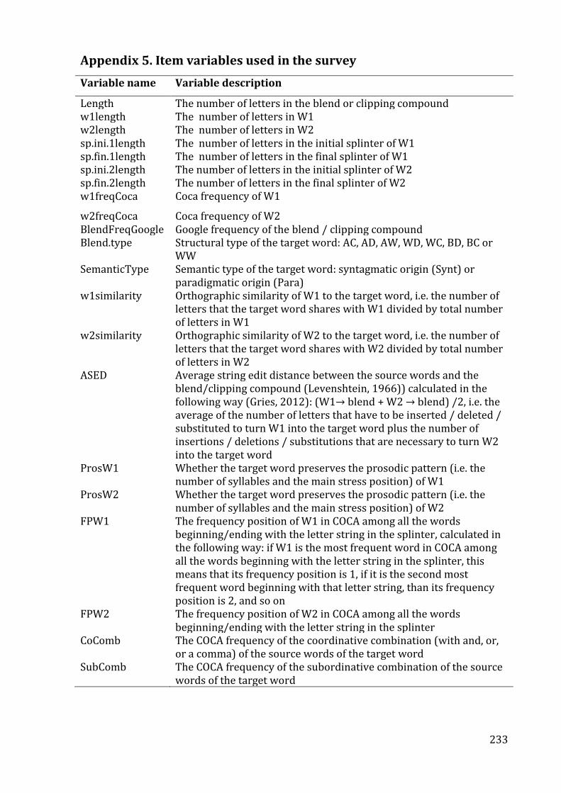
233

Appendix 5. Item variables used in the survey

Variable name Variable description

Length The number of letters in the blend or clipping compound w1length The number of letters in W1 w2length The number of letters in W2 sp.ini.1length The number of letters in the initial splinter of W1 sp.fin.1length The number of letters in the final splinter of W1 sp.ini.2length The number of letters in the initial splinter of W2 sp.fin.2length The number of letters in the final splinter of W2 w1freqCoca Coca frequency of W1

w2freqCoca Coca frequency of W2 BlendFreqGoogle Google frequency of the blend / clipping compound Blend.type Structural type of the target word: AC, AD, AW, WD, WC, BD, BC or

WW SemanticType Semantic type of the target word: syntagmatic origin (Synt) or

paradigmatic origin (Para) w1similarity Orthographic similarity of W1 to the target word, i.e. the number of

letters that the target word shares with W1 divided by total number of letters in W1

w2similarity Orthographic similarity of W2 to the target word, i.e. the number of letters that the target word shares with W2 divided by total number of letters in W2

ASED Average string edit distance between the source words and the blend/clipping compound (Levenshtein, 1966)) calculated in the following way (Gries, 2012): (W1→ blend + W2 → blend) /2, i.e. the average of the number of letters that have to be inserted / deleted / substituted to turn W1 into the target word plus the number of insertions / deletions / substitutions that are necessary to turn W2 into the target word

ProsW1 Whether the target word preserves the prosodic pattern (i.e. the number of syllables and the main stress position) of W1

ProsW2 Whether the target word preserves the prosodic pattern (i.e. the number of syllables and the main stress position) of W2

FPW1 The frequency position of W1 in COCA among all the words beginning/ending with the letter string in the splinter, calculated in the following way: if W1 is the most frequent word in COCA among all the words beginning with the letter string in the splinter, this means that its frequency position is 1, if it is the second most frequent word beginning with that letter string, than its frequency position is 2, and so on

FPW2 The frequency position of W2 in COCA among all the words beginning/ending with the letter string in the splinter

CoComb The COCA frequency of the coordinative combination (with and, or, or a comma) of the source words of the target word

SubComb The COCA frequency of the subordinative combination of the source words of the target word

234

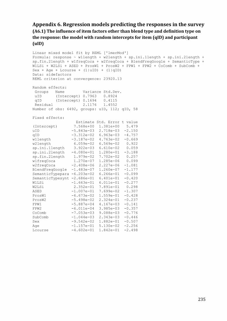
235

Appendix 6. Regression models predicting the responses in the survey (A6.1) The influence of item factors other than blend type and definition type on

the response: the model with random intercepts for item (qID) and participant

(uID)

Linear mixed model fit by REML ['lmerMod']

Formula: response ~ w1length + w2length + sp.ini.1length + sp.ini.2length +

sp.fin.2length + w1freqCoca + w2freqCoca + BlendFreqGoogle + SemanticType +

W1LSi + W2LSi + ASED + ProsW1 + ProsW2 + FPW1 + FPW2 + CoComb + SubComb +

Sex + Age + Lcourse + (1|uID) + (1|qID)

Data: sidefactors

REML criterion at convergence: 23920.13

Random effects:

Groups Name Variance Std.Dev.

uID (Intercept) 0.7963 0.8924

qID (Intercept) 0.1694 0.4115

Residual 2.1176 1.4552

Number of obs: 6492, groups: uID, 112; qID, 58

Fixed effects:

Estimate Std. Error t value

(Intercept) 7.568e+00 1.381e+00 5.479

uID -5.843e-03 2.718e-03 -2.150

qID -3.312e-02 6.963e-03 -4.757

w1length -3.187e-02 4.763e-02 -0.669

w2length 6.059e-02 6.569e-02 0.922

sp.ini.1length 3.922e-03 6.610e-02 0.059

sp.ini.2length -4.080e-01 1.280e-01 -3.188

sp.fin.2length 1.979e-02 7.702e-02 0.257

w1freqCoca 1.270e-07 1.285e-06 0.099

w2freqCoca -2.408e-06 2.227e-06 -1.081

BlendFreqGoogle -1.483e-07 1.260e-07 -1.177

SemanticTypepara -6.203e-02 6.266e-01 -0.099

SemanticTypesynt -2.686e-01 6.401e-01 -0.420

W1LSi -1.663e-01 6.011e-01 -0.277

W2LSi 2.352e-01 7.891e-01 0.298

ASED -1.007e-01 7.699e-02 -1.307

ProsW1 -6.673e-02 1.559e-01 -0.428

ProsW2 -5.498e-02 2.324e-01 -0.237

FPW1 -5.887e-04 4.167e-03 -0.141

FPW2 -6.011e-04 3.985e-03 -0.357

CoComb -7.053e-03 9.088e-03 -0.776

SubComb -1.044e-03 2.343e-03 -0.446

Sex -9.542e-02 1.882e-01 -0.507

Age -1.157e-01 5.130e-02 -2.256

Lcourse -4.602e-01 1.842e-01 -2.498

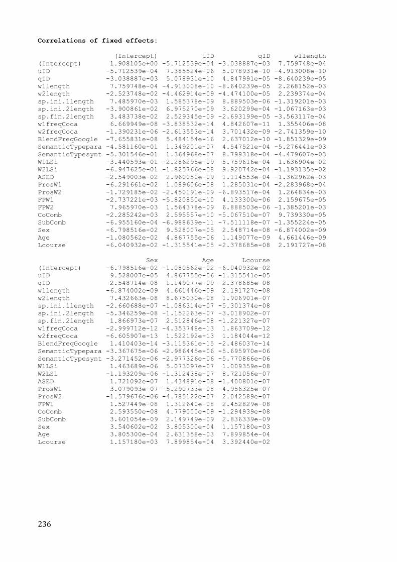
236

Correlations of fixed effects:

(Intercept) uID qID w1length

(Intercept) 1.908105e+00 -5.712539e-04 -3.038887e-03 7.759748e-04

uID -5.712539e-04 7.385524e-06 5.078931e-10 -4.913008e-10

qID -3.038887e-03 5.078931e-10 4.847991e-05 -8.640239e-05

w1length 7.759748e-04 -4.913008e-10 -8.640239e-05 2.268152e-03

w2length -2.523748e-02 -4.462914e-09 -4.474100e-05 2.239374e-04

sp.ini.1length 7.485970e-03 1.585378e-09 8.889503e-06 -1.319201e-03

sp.ini.2length -3.900861e-02 6.975270e-09 3.620299e-04 -1.067163e-03

sp.fin.2length 3.483738e-02 2.529345e-09 -2.693199e-05 -3.563117e-04

w1freqCoca 6.669949e-08 -3.838532e-14 4.842607e-11 1.355406e-08

w2freqCoca -1.390231e-06 -2.613553e-14 3.701432e-09 -2.741359e-10

BlendFreqGoogle -7.655831e-08 5.484154e-16 2.637012e-10 -1.851329e-09

SemanticTypepara -4.581160e-01 1.349201e-07 4.547521e-04 -5.276441e-03

SemanticTypesynt -5.301546e-01 1.364968e-07 8.799318e-04 -4.479607e-03

W1LSi -3.440593e-01 -2.286295e-09 5.759616e-04 1.636904e-02

W2LSi -6.947625e-01 -1.825766e-08 9.920742e-04 -1.193135e-02

ASED -2.549003e-02 2.960050e-09 1.114553e-04 -1.362962e-03

ProsW1 -6.291661e-02 1.089606e-08 1.285031e-04 -2.283968e-04

ProsW2 -1.729185e-02 -2.450191e-09 -6.893517e-04 1.264834e-03

FPW1 -2.737221e-03 -5.820850e-10 4.133300e-06 2.159675e-05

FPW2 7.965970e-03 1.564378e-09 6.888503e-06 -1.385201e-03

CoComb -2.285242e-03 2.595557e-10 -5.067510e-07 9.739330e-05

SubComb -6.955160e-04 -6.988639e-11 -7.511118e-07 -1.355224e-05

Sex -6.798516e-02 9.528007e-05 2.548714e-08 -6.874002e-09

Age -1.080562e-02 4.867755e-06 1.149077e-09 4.661446e-09

Lcourse -6.040932e-02 -1.315541e-05 -2.378685e-08 2.191727e-08

Sex Age Lcourse

(Intercept) -6.798516e-02 -1.080562e-02 -6.040932e-02

uID 9.528007e-05 4.867755e-06 -1.315541e-05

qID 2.548714e-08 1.149077e-09 -2.378685e-08

w1length -6.874002e-09 4.661446e-09 2.191727e-08

w2length 7.432663e-08 8.675030e-08 1.906901e-07

sp.ini.1length -2.660688e-07 -1.086314e-07 -5.301374e-08

sp.ini.2length -5.346259e-08 -1.152263e-07 -3.018902e-07

sp.fin.2length 1.866973e-07 2.512846e-08 -1.221327e-07

w1freqCoca -2.999712e-12 -4.353748e-13 1.863709e-12

w2freqCoca -6.605907e-13 1.522192e-13 1.184044e-12

BlendFreqGoogle 1.410403e-14 -3.115361e-15 -2.486037e-14

SemanticTypepara -3.367675e-06 -2.986445e-06 -5.695970e-06

SemanticTypesynt -3.271452e-06 -2.977326e-06 -5.770866e-06

W1LSi 1.463689e-06 5.073097e-07 1.009359e-08

W2LSi -1.193209e-06 -1.312438e-07 8.721056e-07

ASED 1.721092e-07 1.434891e-08 -1.400801e-07

ProsW1 3.079093e-07 -5.290733e-08 -4.956325e-07

ProsW2 -1.579676e-06 -4.785122e-07 2.042589e-07

FPW1 1.527449e-08 1.312640e-08 2.452829e-08

CoComb 2.593550e-08 4.779000e-09 -1.294939e-08

SubComb 3.601054e-09 2.149749e-09 2.836339e-09

Sex 3.540602e-02 3.805300e-04 1.157180e-03

Age 3.805300e-04 2.631358e-03 7.899854e-04

Lcourse 1.157180e-03 7.899854e-04 3.392440e-02

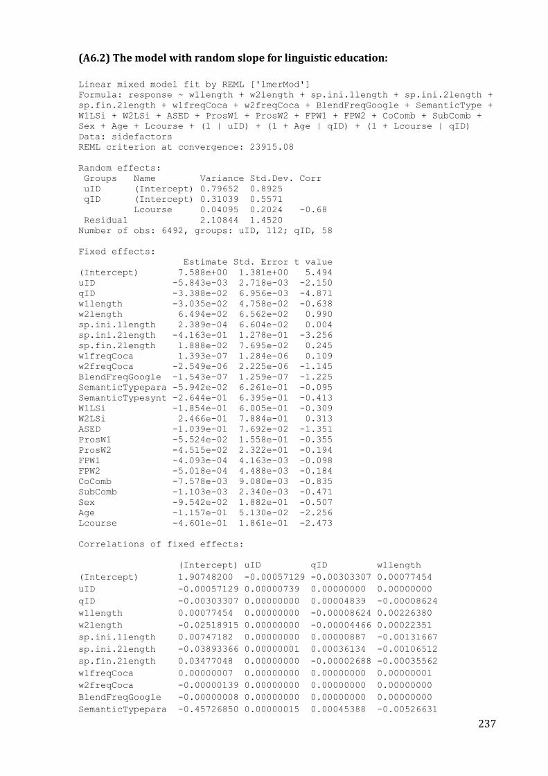
237

(A6.2) The model with random slope for linguistic education:

Linear mixed model fit by REML ['lmerMod']




Sex + Age + Lcourse + (1 | uID) + (1 + Age | qID) + (1 + Lcourse | qID)

Data: sidefactors


Random effects:

Groups Name Variance Std.Dev. Corr



Lcourse 0.04095 0.2024 -0.68

Residual 2.10844 1.4520


Fixed effects:


(Intercept) 7.588e+00 1.381e+00 5.494

uID -5.843e-03 2.718e-03 -2.150

qID -3.388e-02 6.956e-03 -4.871

w1length -3.035e-02 4.758e-02 -0.638

w2length 6.494e-02 6.562e-02 0.990

sp.ini.1length 2.389e-04 6.604e-02 0.004

sp.ini.2length -4.163e-01 1.278e-01 -3.256

sp.fin.2length 1.888e-02 7.695e-02 0.245

w1freqCoca 1.393e-07 1.284e-06 0.109

w2freqCoca -2.549e-06 2.225e-06 -1.145




W1LSi -1.854e-01 6.005e-01 -0.309

W2LSi 2.466e-01 7.884e-01 0.313

ASED -1.039e-01 7.692e-02 -1.351

ProsW1 -5.524e-02 1.558e-01 -0.355

ProsW2 -4.515e-02 2.322e-01 -0.194

FPW1 -4.093e-04 4.163e-03 -0.098

FPW2 -5.018e-04 4.488e-03 -0.184

CoComb -7.578e-03 9.080e-03 -0.835

SubComb -1.103e-03 2.340e-03 -0.471

Sex -9.542e-02 1.882e-01 -0.507

Age -1.157e-01 5.130e-02 -2.256

Lcourse -4.601e-01 1.861e-01 -2.473

Correlations of fixed effects:


(Intercept) 1.90748200 -0.00057129 -0.00303307 0.00077454

uID -0.00057129 0.00000739 0.00000000 0.00000000

qID -0.00303307 0.00000000 0.00004839 -0.00008624

w1length 0.00077454 0.00000000 -0.00008624 0.00226380

w2length -0.02518915 0.00000000 -0.00004466 0.00022351

sp.ini.1length 0.00747182 0.00000000 0.00000887 -0.00131667

sp.ini.2length -0.03893366 0.00000001 0.00036134 -0.00106512

sp.fin.2length 0.03477048 0.00000000 -0.00002688 -0.00035562

w1freqCoca 0.00000007 0.00000000 0.00000000 0.00000001

w2freqCoca -0.00000139 0.00000000 0.00000000 0.00000000

BlendFreqGoogle -0.00000008 0.00000000 0.00000000 0.00000000

SemanticTypepara -0.45726850 0.00000015 0.00045388 -0.00526631

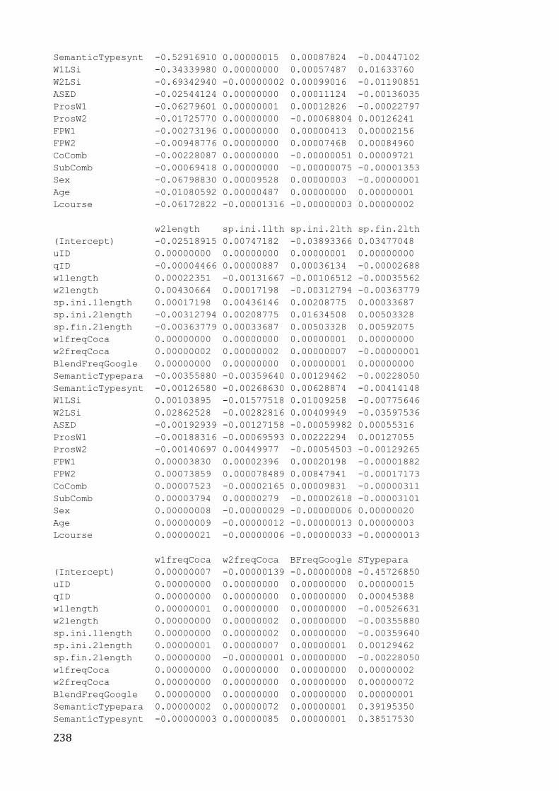
238

SemanticTypesynt -0.52916910 0.00000015 0.00087824 -0.00447102

W1LSi -0.34339980 0.00000000 0.00057487 0.01633760

W2LSi -0.69342940 -0.00000002 0.00099016 -0.01190851

ASED -0.02544124 0.00000000 0.00011124 -0.00136035

ProsW1 -0.06279601 0.00000001 0.00012826 -0.00022797

ProsW2 -0.01725770 0.00000000 -0.00068804 0.00126241

FPW1 -0.00273196 0.00000000 0.00000413 0.00002156

FPW2 -0.00948776 0.00000000 0.00007468 0.00084960

CoComb -0.00228087 0.00000000 -0.00000051 0.00009721

SubComb -0.00069418 0.00000000 -0.00000075 -0.00001353

Sex -0.06798830 0.00009528 0.00000003 -0.00000001

Age -0.01080592 0.00000487 0.00000000 0.00000001

Lcourse -0.06172822 -0.00001316 -0.00000003 0.00000002

w2length sp.ini.1lth sp.ini.2lth sp.fin.2lth

(Intercept) -0.02518915 0.00747182 -0.03893366 0.03477048

uID 0.00000000 0.00000000 0.00000001 0.00000000

qID -0.00004466 0.00000887 0.00036134 -0.00002688

w1length 0.00022351 -0.00131667 -0.00106512 -0.00035562

w2length 0.00430664 0.00017198 -0.00312794 -0.00363779

sp.ini.1length 0.00017198 0.00436146 0.00208775 0.00033687

sp.ini.2length -0.00312794 0.00208775 0.01634508 0.00503328

sp.fin.2length -0.00363779 0.00033687 0.00503328 0.00592075

w1freqCoca 0.00000000 0.00000000 0.00000001 0.00000000

w2freqCoca 0.00000002 0.00000002 0.00000007 -0.00000001

BlendFreqGoogle 0.00000000 0.00000000 0.00000001 0.00000000

SemanticTypepara -0.00355880 -0.00359640 0.00129462 -0.00228050

SemanticTypesynt -0.00126580 -0.00268630 0.00628874 -0.00414148

W1LSi 0.00103895 -0.01577518 0.01009258 -0.00775646

W2LSi 0.02862528 -0.00282816 0.00409949 -0.03597536

ASED -0.00192939 -0.00127158 -0.00059982 0.00055316

ProsW1 -0.00188316 -0.00069593 0.00222294 0.00127055

ProsW2 -0.00140697 0.00449977 -0.00054503 -0.00129265

FPW1 0.00003830 0.00002396 0.00020198 -0.00001882

FPW2 0.00073859 0.000078489 0.00847941 -0.00017173

CoComb 0.00007523 -0.00002165 0.00009831 -0.00000311

SubComb 0.00003794 0.00000279 -0.00002618 -0.00003101

Sex 0.00000008 -0.00000029 -0.00000006 0.00000020

Age 0.00000009 -0.00000012 -0.00000013 0.00000003

Lcourse 0.00000021 -0.00000006 -0.00000033 -0.00000013

w1freqCoca w2freqCoca BFreqGoogle STypepara

(Intercept) 0.00000007 -0.00000139 -0.00000008 -0.45726850

uID 0.00000000 0.00000000 0.00000000 0.00000015

qID 0.00000000 0.00000000 0.00000000 0.00045388

w1length 0.00000001 0.00000000 0.00000000 -0.00526631

w2length 0.00000000 0.00000002 0.00000000 -0.00355880

sp.ini.1length 0.00000000 0.00000002 0.00000000 -0.00359640

sp.ini.2length 0.00000001 0.00000007 0.00000001 0.00129462

sp.fin.2length 0.00000000 -0.00000001 0.00000000 -0.00228050

w1freqCoca 0.00000000 0.00000000 0.00000000 0.00000002

w2freqCoca 0.00000000 0.00000000 0.00000000 0.00000072


SemanticTypepara 0.00000002 0.00000072 0.00000001 0.39195350

SemanticTypesynt -0.00000003 0.00000085 0.00000001 0.38517530

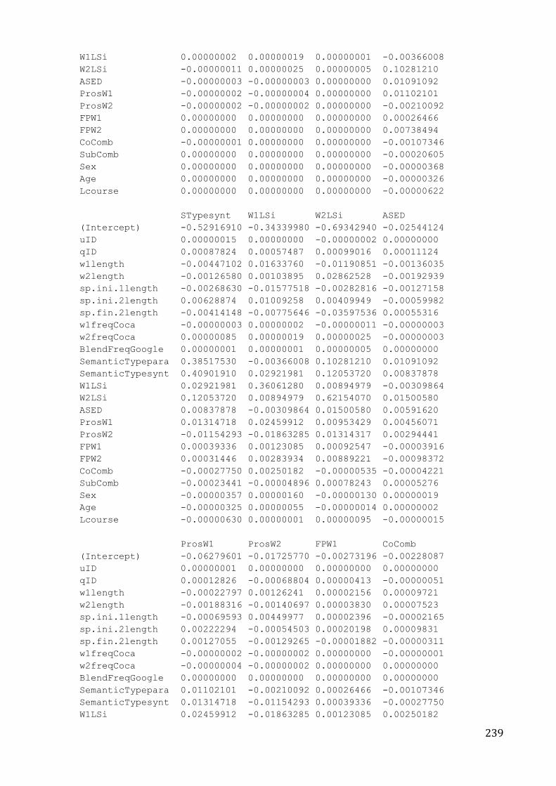
239

W1LSi 0.00000002 0.00000019 0.00000001 -0.00366008

W2LSi -0.00000011 0.00000025 0.00000005 0.10281210

ASED -0.00000003 -0.00000003 0.00000000 0.01091092

ProsW1 -0.00000002 -0.00000004 0.00000000 0.01102101

ProsW2 -0.00000002 -0.00000002 0.00000000 -0.00210092

FPW1 0.00000000 0.00000000 0.00000000 0.00026466

FPW2 0.00000000 0.00000000 0.00000000 0.00738494

CoComb -0.00000001 0.00000000 0.00000000 -0.00107346

SubComb 0.00000000 0.00000000 0.00000000 -0.00020605

Sex 0.00000000 0.00000000 0.00000000 -0.00000368

Age 0.00000000 0.00000000 0.00000000 -0.00000326

Lcourse 0.00000000 0.00000000 0.00000000 -0.00000622

STypesynt W1LSi W2LSi ASED

(Intercept) -0.52916910 -0.34339980 -0.69342940 -0.02544124

uID 0.00000015 0.00000000 -0.00000002 0.00000000

qID 0.00087824 0.00057487 0.00099016 0.00011124

w1length -0.00447102 0.01633760 -0.01190851 -0.00136035

w2length -0.00126580 0.00103895 0.02862528 -0.00192939

sp.ini.1length -0.00268630 -0.01577518 -0.00282816 -0.00127158

sp.ini.2length 0.00628874 0.01009258 0.00409949 -0.00059982

sp.fin.2length -0.00414148 -0.00775646 -0.03597536 0.00055316

w1freqCoca -0.00000003 0.00000002 -0.00000011 -0.00000003

w2freqCoca 0.00000085 0.00000019 0.00000025 -0.00000003


SemanticTypepara 0.38517530 -0.00366008 0.10281210 0.01091092

SemanticTypesynt 0.40901910 0.02921981 0.12053720 0.00837878

W1LSi 0.02921981 0.36061280 0.00894979 -0.00309864

W2LSi 0.12053720 0.00894979 0.62154070 0.01500580

ASED 0.00837878 -0.00309864 0.01500580 0.00591620

ProsW1 0.01314718 0.02459912 0.00953429 0.00456071

ProsW2 -0.01154293 -0.01863285 0.01314317 0.00294441

FPW1 0.00039336 0.00123085 0.00092547 -0.00003916

FPW2 0.00031446 0.00283934 0.00889221 -0.00098372

CoComb -0.00027750 0.00250182 -0.00000535 -0.00004221

SubComb -0.00023441 -0.00004896 0.00078243 0.00005276

Sex -0.00000357 0.00000160 -0.00000130 0.00000019

Age -0.00000325 0.00000055 -0.00000014 0.00000002

Lcourse -0.00000630 0.00000001 0.00000095 -0.00000015

ProsW1 ProsW2 FPW1 CoComb

(Intercept) -0.06279601 -0.01725770 -0.00273196 -0.00228087

uID 0.00000001 0.00000000 0.00000000 0.00000000

qID 0.00012826 -0.00068804 0.00000413 -0.00000051

w1length -0.00022797 0.00126241 0.00002156 0.00009721

w2length -0.00188316 -0.00140697 0.00003830 0.00007523

sp.ini.1length -0.00069593 0.00449977 0.00002396 -0.00002165

sp.ini.2length 0.00222294 -0.00054503 0.00020198 0.00009831

sp.fin.2length 0.00127055 -0.00129265 -0.00001882 -0.00000311

w1freqCoca -0.00000002 -0.00000002 0.00000000 -0.00000001

w2freqCoca -0.00000004 -0.00000002 0.00000000 0.00000000


SemanticTypepara 0.01102101 -0.00210092 0.00026466 -0.00107346

SemanticTypesynt 0.01314718 -0.01154293 0.00039336 -0.00027750

W1LSi 0.02459912 -0.01863285 0.00123085 0.00250182

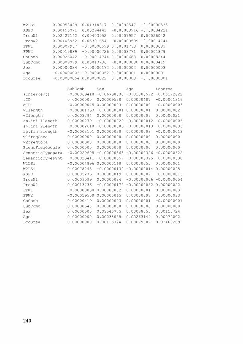
240

W2LSi 0.00953429 0.01314317 0.00092547 -0.00000535

ASED 0.00456071 0.00294441 -0.00003916 -0.00004221

ProsW1 0.02427142 0.00403952 0.00007957 0.00026042

ProsW2 0.00403952 0.05391654 -0.00000599 -0.00014744

FPW1 0.00007957 -0.00000599 0.00001733 0.00000683

FPW2 0.00019889 -0.00000726 0.00003771 0.00001879

CoComb 0.00026042 -0.00014744 0.00000683 0.00008244

SubComb 0.00009099 0.00013736 -0.00000030 0.00000419

Sex 0.00000034 -0.00000172 0.00000002 0.00000003

Age -0.00000006 -0.00000052 0.00000001 0.00000001

Lcourse -0.00000054 0.00000022 0.00000003 -0.00000001

SubComb Sex Age Lcourse

(Intercept) -0.00069418 -0.06798830 -0.01080592 -0.06172822

uID 0.00000000 0.00009528 0.00000487 -0.00001316

qID -0.00000075 0.00000003 0.00000000 -0.00000003

w1length -0.00001353 -0.00000001 0.00000001 0.00000002

w2length 0.00003794 0.00000008 0.00000009 0.00000021

sp.ini.1length 0.00000279 -0.00000029 -0.00000012 -0.00000006

sp.ini.2length -0.00002618 -0.00000006 -0.00000013 -0.00000033

sp.fin.2length -0.00003101 0.00000020 0.00000003 -0.00000013

w1freqCoca 0.00000000 0.00000000 0.00000000 0.00000000

w2freqCoca 0.00000000 0.00000000 0.00000000 0.00000000


SemanticTypepara -0.00020605 -0.00000368 -0.00000326 -0.00000622

SemanticTypesynt -0.00023441 -0.00000357 -0.00000325 -0.00000630

W1LSi -0.00004896 0.00000160 0.00000055 0.00000001

W2LSi 0.00078243 -0.00000130 -0.00000014 0.00000095

ASED 0.00005276 0.00000019 0.00000002 -0.00000015

ProsW1 0.00009099 0.00000034 -0.00000006 -0.00000054

ProsW2 0.00013736 -0.00000172 -0.00000052 0.00000022

FPW1 -0.00000030 0.00000002 0.00000001 0.00000003

FPW2 -0.00019559 0.00000065 0.00000097 0.00000033

CoComb 0.00000419 0.00000003 0.00000001 -0.00000001

SubComb 0.00000548 0.00000000 0.00000000 0.00000000

Sex 0.00000000 0.03540775 0.00038055 0.00115724

Age 0.00000000 0.00038055 0.00263149 0.00079002

Lcourse 0.00000000 0.00115724 0.00079002 0.03463209

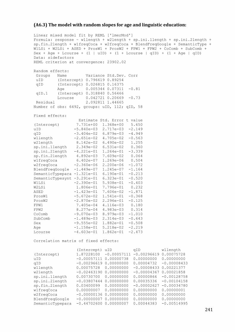
241

(A6.3) The model with random slopes for age and linguistic education: Linear mixed model fit by REML ['lmerMod']




Sex + Age + Lcourse + (1 | uID) + (1 + Lcourse | qID) + (1 + Age | qID)

Data: sidefactors


Random effects:


uID (Intercept) 0.796619 0.89254

qID (Intercept) 0.026815 0.16375

Age 0.005344 0.07311 -0.81

qID.1 (Intercept) 0.318840 0.56466

Lcourse 0.042721 0.20669 -0.73

Residual 2.092811 1.44665


Fixed effects:


(Intercept) 7.731e+00 1.368e+00 5.650

uID -5.840e-03 2.717e-03 -2.149

qID -3.404e-02 6.879e-03 -4.949

w1length -2.651e-02 4.705e-02 -0.563

w2length 8.142e-02 6.490e-02 1.255

sp.ini.1length 2.349e-02 6.531e-02 0.360

sp.ini.2length -4.221e-01 1.264e-01 -3.339

sp.fin.2length 4.892e-03 7.609e-02 0.064

w1freqCoca 6.402e-07 1.269e-06 0.504

w2freqCoca -2.360e-06 2.200e-06 -1.072




W1LSi -2.390e-01 5.938e-01 -0.403

W2LSi 1.806e-01 7.796e-01 0.232

ASED -1.423e-01 7.606e-02 -1.871

ProsW1 -5.672e-02 1.541e-01 -0.368

ProsW2 -2.870e-02 2.296e-01 -0.125

FPW1 7.405e-04 4.116e-03 0.180

FPW2 8.277e-04 4.983e-03 0.314

CoComb -9.070e-03 8.979e-03 -1.010

SubComb -1.489e-03 2.314e-03 -0.643

Sex -9.555e-02 1.882e-01 -0.508

Age -1.158e-01 5.218e-02 -2.219

Lcourse -4.603e-01 1.862e-01 -2.473

Correlation matrix of fixed effects:


(Intercept) 1.87228100 -0.00057111 -0.00296619 0.00075728

uID -0.00057111 0.00000738 0.00000000 0.00000000

qID -0.00296619 0.00000000 0.00004732 -0.00008433

w1length 0.00075728 0.00000000 -0.00008433 0.00221377

w2length -0.02463190 0.00000000 -0.00004367 0.00021858

sp.ini.1length 0.00730700 0.00000000 0.00000866 -0.00128758

sp.ini.2length -0.03807444 0.00000000 0.00035336 -0.00104158

sp.fin.2length 0.03400099 0.00000000 -0.00002627 -0.00034780

w1freqCoca 0.00000007 0.00000000 0.00000000 0.00000001

w2freqCoca -0.00000136 0.00000000 0.00000000 0.00000000

BlendFreqGoogle -0.00000007 0.00000000 0.00000000 0.00000000

SemanticTypepara -0.44702600 0.00000007 0.00044383 -0.00514995

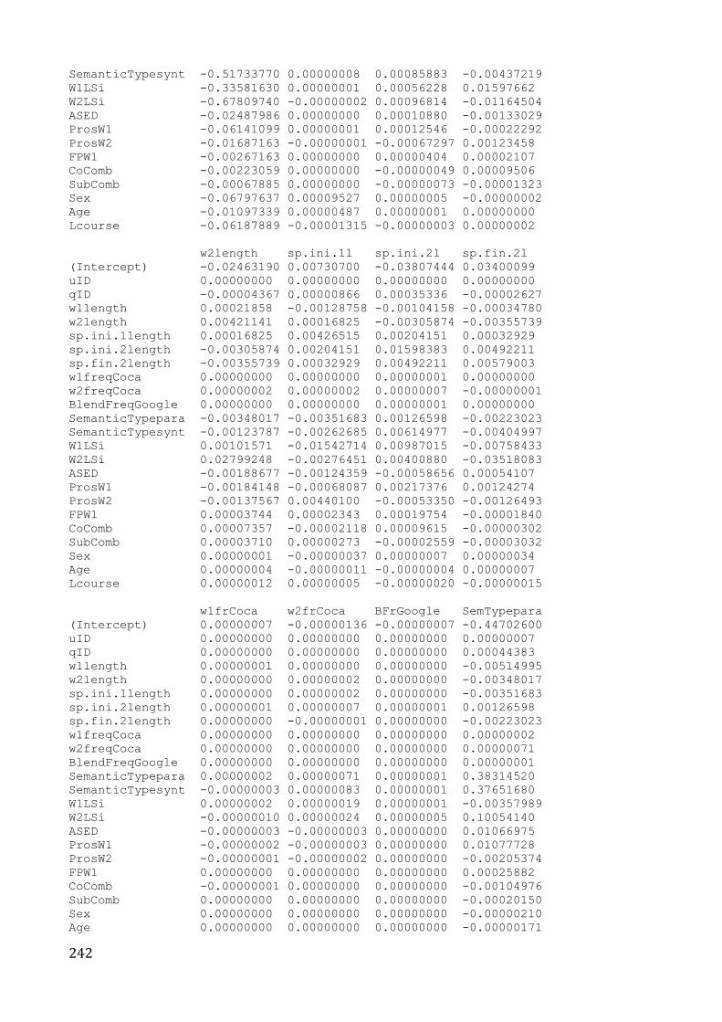
242

SemanticTypesynt -0.51733770 0.00000008 0.00085883 -0.00437219

W1LSi -0.33581630 0.00000001 0.00056228 0.01597662

W2LSi -0.67809740 -0.00000002 0.00096814 -0.01164504

ASED -0.02487986 0.00000000 0.00010880 -0.00133029

ProsW1 -0.06141099 0.00000001 0.00012546 -0.00022292

ProsW2 -0.01687163 -0.00000001 -0.00067297 0.00123458

FPW1 -0.00267163 0.00000000 0.00000404 0.00002107

CoComb -0.00223059 0.00000000 -0.00000049 0.00009506

SubComb -0.00067885 0.00000000 -0.00000073 -0.00001323

Sex -0.06797637 0.00009527 0.00000005 -0.00000002

Age -0.01097339 0.00000487 0.00000001 0.00000000

Lcourse -0.06187889 -0.00001315 -0.00000003 0.00000002

w2length sp.ini.1l sp.ini.2l sp.fin.2l

(Intercept) -0.02463190 0.00730700 -0.03807444 0.03400099

uID 0.00000000 0.00000000 0.00000000 0.00000000

qID -0.00004367 0.00000866 0.00035336 -0.00002627

w1length 0.00021858 -0.00128758 -0.00104158 -0.00034780

w2length 0.00421141 0.00016825 -0.00305874 -0.00355739

sp.ini.1length 0.00016825 0.00426515 0.00204151 0.00032929

sp.ini.2length -0.00305874 0.00204151 0.01598383 0.00492211

sp.fin.2length -0.00355739 0.00032929 0.00492211 0.00579003

w1freqCoca 0.00000000 0.00000000 0.00000001 0.00000000

w2freqCoca 0.00000002 0.00000002 0.00000007 -0.00000001


SemanticTypepara -0.00348017 -0.00351683 0.00126598 -0.00223023

SemanticTypesynt -0.00123787 -0.00262685 0.00614977 -0.00404997

W1LSi 0.00101571 -0.01542714 0.00987015 -0.00758433

W2LSi 0.02799248 -0.00276451 0.00400880 -0.03518083

ASED -0.00188677 -0.00124359 -0.00058656 0.00054107

ProsW1 -0.00184148 -0.00068087 0.00217376 0.00124274

ProsW2 -0.00137567 0.00440100 -0.00053350 -0.00126493

FPW1 0.00003744 0.00002343 0.00019754 -0.00001840

CoComb 0.00007357 -0.00002118 0.00009615 -0.00000302

SubComb 0.00003710 0.00000273 -0.00002559 -0.00003032

Sex 0.00000001 -0.00000037 0.00000007 0.00000034

Age 0.00000004 -0.00000011 -0.00000004 0.00000007

Lcourse 0.00000012 0.00000005 -0.00000020 -0.00000015

w1frCoca w2frCoca BFrGoogle SemTypepara

(Intercept) 0.00000007 -0.00000136 -0.00000007 -0.44702600

uID 0.00000000 0.00000000 0.00000000 0.00000007

qID 0.00000000 0.00000000 0.00000000 0.00044383

w1length 0.00000001 0.00000000 0.00000000 -0.00514995

w2length 0.00000000 0.00000002 0.00000000 -0.00348017

sp.ini.1length 0.00000000 0.00000002 0.00000000 -0.00351683

sp.ini.2length 0.00000001 0.00000007 0.00000001 0.00126598

sp.fin.2length 0.00000000 -0.00000001 0.00000000 -0.00223023

w1freqCoca 0.00000000 0.00000000 0.00000000 0.00000002

w2freqCoca 0.00000000 0.00000000 0.00000000 0.00000071


SemanticTypepara 0.00000002 0.00000071 0.00000001 0.38314520

SemanticTypesynt -0.00000003 0.00000083 0.00000001 0.37651680

W1LSi 0.00000002 0.00000019 0.00000001 -0.00357989

W2LSi -0.00000010 0.00000024 0.00000005 0.10054140

ASED -0.00000003 -0.00000003 0.00000000 0.01066975

ProsW1 -0.00000002 -0.00000003 0.00000000 0.01077728

ProsW2 -0.00000001 -0.00000002 0.00000000 -0.00205374

FPW1 0.00000000 0.00000000 0.00000000 0.00025882

CoComb -0.00000001 0.00000000 0.00000000 -0.00104976

SubComb 0.00000000 0.00000000 0.00000000 -0.00020150

Sex 0.00000000 0.00000000 0.00000000 -0.00000210

Age 0.00000000 0.00000000 0.00000000 -0.00000171

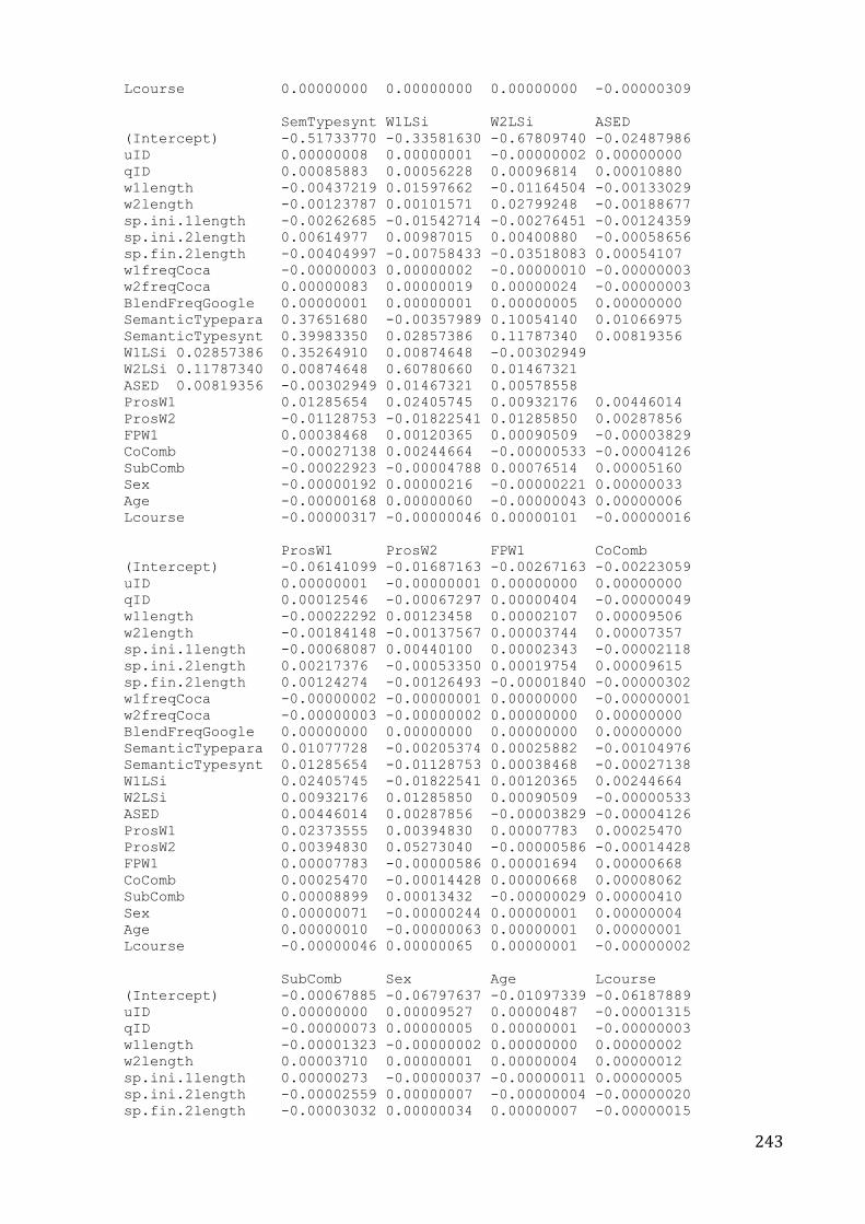
243

Lcourse 0.00000000 0.00000000 0.00000000 -0.00000309

SemTypesynt W1LSi W2LSi ASED

(Intercept) -0.51733770 -0.33581630 -0.67809740 -0.02487986

uID 0.00000008 0.00000001 -0.00000002 0.00000000

qID 0.00085883 0.00056228 0.00096814 0.00010880

w1length -0.00437219 0.01597662 -0.01164504 -0.00133029

w2length -0.00123787 0.00101571 0.02799248 -0.00188677

sp.ini.1length -0.00262685 -0.01542714 -0.00276451 -0.00124359

sp.ini.2length 0.00614977 0.00987015 0.00400880 -0.00058656

sp.fin.2length -0.00404997 -0.00758433 -0.03518083 0.00054107

w1freqCoca -0.00000003 0.00000002 -0.00000010 -0.00000003

w2freqCoca 0.00000083 0.00000019 0.00000024 -0.00000003


SemanticTypepara 0.37651680 -0.00357989 0.10054140 0.01066975

SemanticTypesynt 0.39983350 0.02857386 0.11787340 0.00819356

W1LSi 0.02857386 0.35264910 0.00874648 -0.00302949

W2LSi 0.11787340 0.00874648 0.60780660 0.01467321

ASED 0.00819356 -0.00302949 0.01467321 0.00578558

ProsW1 0.01285654 0.02405745 0.00932176 0.00446014

ProsW2 -0.01128753 -0.01822541 0.01285850 0.00287856

FPW1 0.00038468 0.00120365 0.00090509 -0.00003829

CoComb -0.00027138 0.00244664 -0.00000533 -0.00004126

SubComb -0.00022923 -0.00004788 0.00076514 0.00005160

Sex -0.00000192 0.00000216 -0.00000221 0.00000033

Age -0.00000168 0.00000060 -0.00000043 0.00000006

Lcourse -0.00000317 -0.00000046 0.00000101 -0.00000016

ProsW1 ProsW2 FPW1 CoComb

(Intercept) -0.06141099 -0.01687163 -0.00267163 -0.00223059

uID 0.00000001 -0.00000001 0.00000000 0.00000000

qID 0.00012546 -0.00067297 0.00000404 -0.00000049

w1length -0.00022292 0.00123458 0.00002107 0.00009506

w2length -0.00184148 -0.00137567 0.00003744 0.00007357

sp.ini.1length -0.00068087 0.00440100 0.00002343 -0.00002118

sp.ini.2length 0.00217376 -0.00053350 0.00019754 0.00009615

sp.fin.2length 0.00124274 -0.00126493 -0.00001840 -0.00000302

w1freqCoca -0.00000002 -0.00000001 0.00000000 -0.00000001

w2freqCoca -0.00000003 -0.00000002 0.00000000 0.00000000


SemanticTypepara 0.01077728 -0.00205374 0.00025882 -0.00104976

SemanticTypesynt 0.01285654 -0.01128753 0.00038468 -0.00027138

W1LSi 0.02405745 -0.01822541 0.00120365 0.00244664

W2LSi 0.00932176 0.01285850 0.00090509 -0.00000533

ASED 0.00446014 0.00287856 -0.00003829 -0.00004126

ProsW1 0.02373555 0.00394830 0.00007783 0.00025470

ProsW2 0.00394830 0.05273040 -0.00000586 -0.00014428

FPW1 0.00007783 -0.00000586 0.00001694 0.00000668

CoComb 0.00025470 -0.00014428 0.00000668 0.00008062

SubComb 0.00008899 0.00013432 -0.00000029 0.00000410

Sex 0.00000071 -0.00000244 0.00000001 0.00000004

Age 0.00000010 -0.00000063 0.00000001 0.00000001

Lcourse -0.00000046 0.00000065 0.00000001 -0.00000002

SubComb Sex Age Lcourse

(Intercept) -0.00067885 -0.06797637 -0.01097339 -0.06187889

uID 0.00000000 0.00009527 0.00000487 -0.00001315

qID -0.00000073 0.00000005 0.00000001 -0.00000003

w1length -0.00001323 -0.00000002 0.00000000 0.00000002

w2length 0.00003710 0.00000001 0.00000004 0.00000012

sp.ini.1length 0.00000273 -0.00000037 -0.00000011 0.00000005

sp.ini.2length -0.00002559 0.00000007 -0.00000004 -0.00000020

sp.fin.2length -0.00003032 0.00000034 0.00000007 -0.00000015

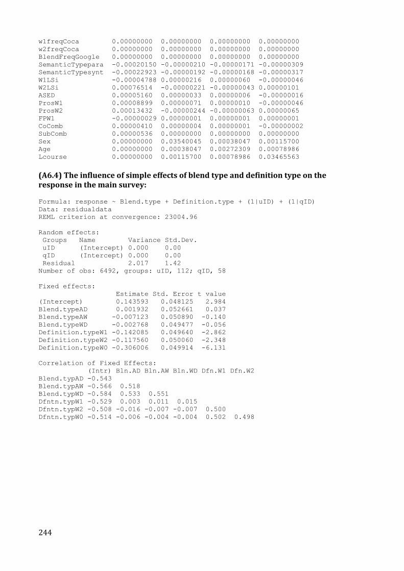
244

w1freqCoca 0.00000000 0.00000000 0.00000000 0.00000000

w2freqCoca 0.00000000 0.00000000 0.00000000 0.00000000


SemanticTypepara -0.00020150 -0.00000210 -0.00000171 -0.00000309

SemanticTypesynt -0.00022923 -0.00000192 -0.00000168 -0.00000317

W1LSi -0.00004788 0.00000216 0.00000060 -0.00000046

W2LSi 0.00076514 -0.00000221 -0.00000043 0.00000101

ASED 0.00005160 0.00000033 0.00000006 -0.00000016

ProsW1 0.00008899 0.00000071 0.00000010 -0.00000046

ProsW2 0.00013432 -0.00000244 -0.00000063 0.00000065

FPW1 -0.00000029 0.00000001 0.00000001 0.00000001

CoComb 0.00000410 0.00000004 0.00000001 -0.00000002

SubComb 0.00000536 0.00000000 0.00000000 0.00000000

Sex 0.00000000 0.03540045 0.00038047 0.00115700

Age 0.00000000 0.00038047 0.00272309 0.00078986

Lcourse 0.00000000 0.00115700 0.00078986 0.03465563

(A6.4) The influence of simple effects of blend type and definition type on the response in the main survey:

Formula: response ~ Blend.type + Definition.type + (1|uID) + (1|qID)

Data: residualdata


Random effects:




Residual 2.017 1.42


Fixed effects:


(Intercept) 0.143593 0.048125 2.984

Blend.typeAD 0.001932 0.052661 0.037

Blend.typeAW -0.007123 0.050890 -0.140

Blend.typeWD -0.002768 0.049477 -0.056

Definition.typeW1 -0.142085 0.049640 -2.862



Correlation of Fixed Effects:

(Intr) Bln.AD Bln.AW Bln.WD Dfn.W1 Dfn.W2

Blend.typAD -0.543

Blend.typAW -0.566 0.518

Blend.typWD -0.584 0.533 0.551

Dfntn.typW1 -0.529 0.003 0.011 0.015

Dfntn.typW2 -0.508 -0.016 -0.007 -0.007 0.500

Dfntn.typW0 -0.514 -0.006 -0.004 -0.004 0.502 0.498

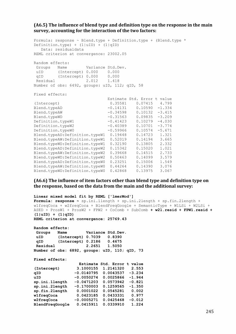
245

(A6.5) The influence of blend type and definition type on the response in the main survey, accounting for the interaction of the two factors:

Formula: response ~ Blend.type + Definition.type + (Blend.type *

Definition.type) + (1|uID) + (1|qID)

Data: residualdata


Random effects:




Residual 2.012 1.418


Fixed effects:


(Intercept) 0.35581 0.07415 4.799

Blend.typeAD -0.14131 0.10590 -1.334

Blend.typeAW -0.34598 0.10132 -3.415

Blend.typeWD -0.31563 0.09835 -3.209




Blend.typeAD:Definition.typeW1 0.19448 0.14723 1.321

Blend.typeAW:Definition.typeW1 0.52019 0.14194 3.665

Blend.typeWD:Definition.typeW1 0.32190 0.13805 2.332







(A6.6) The influence of item factors other than blend type and definition type on the response, based on the data from the main and the additional survey: Linear mixed model fit by REML ['lmerMod']

Formula: response ~ sp.ini.1length + sp.ini.2length + sp.fin.2length +

w1freqCoca + w2freqCoca + BlendFreqGoogle + SemanticType + W1LSi + W2LSi +

ASED + ProsW1 + ProsW2 + FPW2 + CoComb + SubComb + w2l.resid + FPW1.resid +

(1|uID) + (1|qID)


Random effects:




Residual 2.2651 1.5050


Fixed effects:


(Intercept) 3.1000155 1.2141320 2.553

qID -0.0140795 0.0043537 -3.234

uID -0.0050274 0.0025866 -1.944

sp.ini.1length -0.0471203 0.0573942 -0.821

sp.ini.2length -0.1700003 0.1259565 -1.350

sp.fin.2length 0.0001022 0.0545281 0.002

w1freqCoca 0.0423185 0.0433331 0.977

w2freqCoca -0.0005271 0.0425468 -0.012

BlendFreqGoogle 0.0415911 0.0339910 1.224

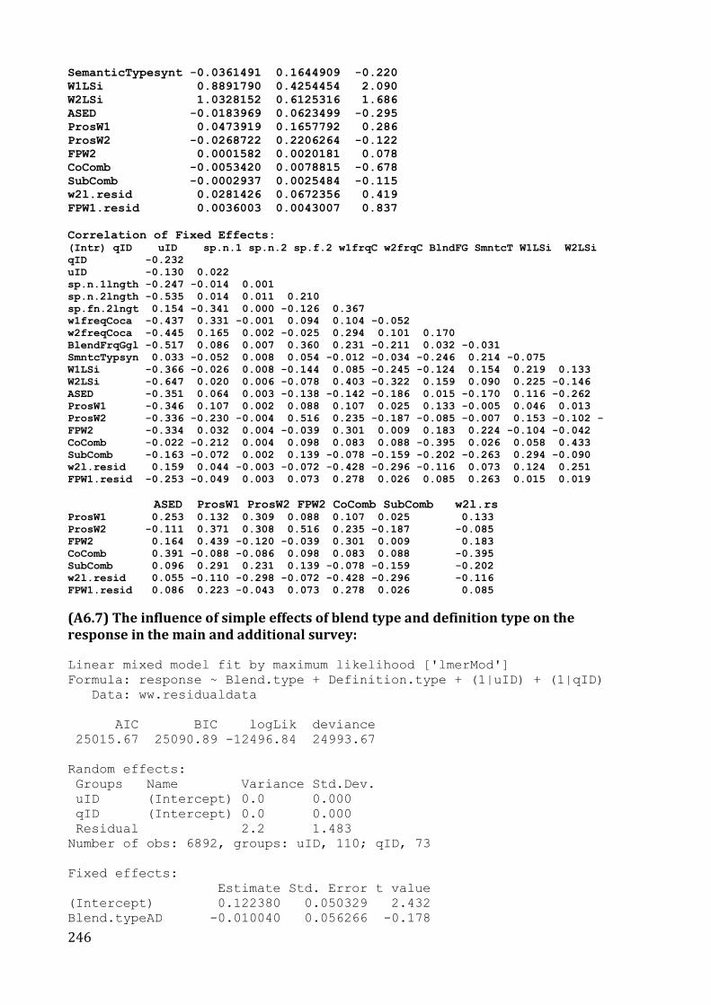
246

SemanticTypesynt -0.0361491 0.1644909 -0.220

W1LSi 0.8891790 0.4254454 2.090

W2LSi 1.0328152 0.6125316 1.686

ASED -0.0183969 0.0623499 -0.295

ProsW1 0.0473919 0.1657792 0.286

ProsW2 -0.0268722 0.2206264 -0.122

FPW2 0.0001582 0.0020181 0.078

CoComb -0.0053420 0.0078815 -0.678

SubComb -0.0002937 0.0025484 -0.115

w2l.resid 0.0281426 0.0672356 0.419

FPW1.resid 0.0036003 0.0043007 0.837

Correlation of Fixed Effects: (Intr) qID uID sp.n.1 sp.n.2 sp.f.2 w1frqC w2frqC BlndFG SmntcT W1LSi W2LSi

qID -0.232

uID -0.130 0.022

sp.n.1lngth -0.247 -0.014 0.001

sp.n.2lngth -0.535 0.014 0.011 0.210

sp.fn.2lngt 0.154 -0.341 0.000 -0.126 0.367

w1freqCoca -0.437 0.331 -0.001 0.094 0.104 -0.052

w2freqCoca -0.445 0.165 0.002 -0.025 0.294 0.101 0.170

BlendFrqGgl -0.517 0.086 0.007 0.360 0.231 -0.211 0.032 -0.031

SmntcTypsyn 0.033 -0.052 0.008 0.054 -0.012 -0.034 -0.246 0.214 -0.075

W1LSi -0.366 -0.026 0.008 -0.144 0.085 -0.245 -0.124 0.154 0.219 0.133

W2LSi -0.647 0.020 0.006 -0.078 0.403 -0.322 0.159 0.090 0.225 -0.146

ASED -0.351 0.064 0.003 -0.138 -0.142 -0.186 0.015 -0.170 0.116 -0.262

ProsW1 -0.346 0.107 0.002 0.088 0.107 0.025 0.133 -0.005 0.046 0.013

ProsW2 -0.336 -0.230 -0.004 0.516 0.235 -0.187 -0.085 -0.007 0.153 -0.102 -

FPW2 -0.334 0.032 0.004 -0.039 0.301 0.009 0.183 0.224 -0.104 -0.042

CoComb -0.022 -0.212 0.004 0.098 0.083 0.088 -0.395 0.026 0.058 0.433

SubComb -0.163 -0.072 0.002 0.139 -0.078 -0.159 -0.202 -0.263 0.294 -0.090

w2l.resid 0.159 0.044 -0.003 -0.072 -0.428 -0.296 -0.116 0.073 0.124 0.251

FPW1.resid -0.253 -0.049 0.003 0.073 0.278 0.026 0.085 0.263 0.015 0.019

ASED ProsW1 ProsW2 FPW2 CoComb SubComb w2l.rs ProsW1 0.253 0.132 0.309 0.088 0.107 0.025 0.133

ProsW2 -0.111 0.371 0.308 0.516 0.235 -0.187 -0.085

FPW2 0.164 0.439 -0.120 -0.039 0.301 0.009 0.183

CoComb 0.391 -0.088 -0.086 0.098 0.083 0.088 -0.395

SubComb 0.096 0.291 0.231 0.139 -0.078 -0.159 -0.202

w2l.resid 0.055 -0.110 -0.298 -0.072 -0.428 -0.296 -0.116

FPW1.resid 0.086 0.223 -0.043 0.073 0.278 0.026 0.085

(A6.7) The influence of simple effects of blend type and definition type on the response in the main and additional survey:

Linear mixed model fit by maximum likelihood ['lmerMod']

Formula: response ~ Blend.type + Definition.type + (1|uID) + (1|qID)

Data: ww.residualdata

AIC BIC logLik deviance

25015.67 25090.89 -12496.84 24993.67

Random effects:




Residual 2.2 1.483


Fixed effects:


(Intercept) 0.122380 0.050329 2.432

Blend.typeAD -0.010040 0.056266 -0.178

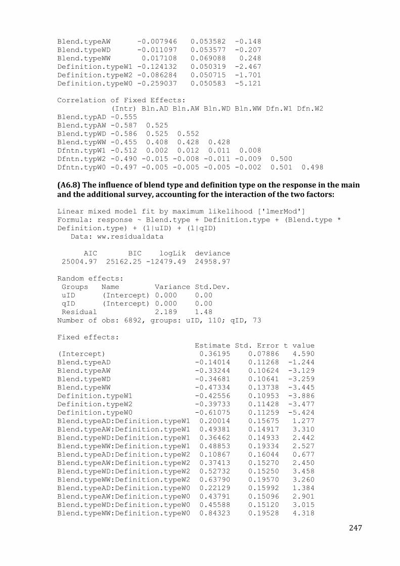
247

Blend.typeAW -0.007946 0.053582 -0.148

Blend.typeWD -0.011097 0.053577 -0.207

Blend.typeWW 0.017108 0.069088 0.248





(Intr) Bln.AD Bln.AW Bln.WD Bln.WW Dfn.W1 Dfn.W2

Blend.typAD -0.555

Blend.typAW -0.587 0.525

Blend.typWD -0.586 0.525 0.552

Blend.typWW -0.455 0.408 0.428 0.428

Dfntn.typW1 -0.512 0.002 0.012 0.011 0.008

Dfntn.typW2 -0.490 -0.015 -0.008 -0.011 -0.009 0.500

Dfntn.typW0 -0.497 -0.005 -0.005 -0.005 -0.002 0.501 0.498

(A6.8) The influence of blend type and definition type on the response in the main and the additional survey, accounting for the interaction of the two factors:

Linear mixed model fit by maximum likelihood ['lmerMod']

Formula: response ~ Blend.type + Definition.type + (Blend.type *

Definition.type) + (1|uID) + (1|qID)

Data: ww.residualdata


25004.97 25162.25 -12479.49 24958.97

Random effects:




Residual 2.189 1.48


Fixed effects:


(Intercept) 0.36195 0.07886 4.590

Blend.typeAD -0.14014 0.11268 -1.244

Blend.typeAW -0.33244 0.10624 -3.129

Blend.typeWD -0.34681 0.10641 -3.259

Blend.typeWW -0.47334 0.13738 -3.445







Blend.typeWW:Definition.typeW1 0.48853 0.19334 2.527









248

249

Appendix 7. Information sheet for the participants of the experiment



tel: 4635600

fax: 4635604




Anna Siyanova: [email protected]

INFORMATION SHEET FOR PARTICIPANTS

Thank you for participating in my study. My name is Natalia Beliaeva and I am a PhD

student in Linguistics at Victoria University of Wellington in New Zealand. I am looking at

how people understand new words that appear in English.

This project has been granted ethical approval by the Victoria University of Wellington

Human Ethics Committee.

I am asking you to agree to take part in a linguistic experiment, during which you will

complete two tasks. First, you will be shown a number of complex words on the computer

screen and will be asked to guess what parts they consist of. Then, you will be shown a series

of word-sized stimuli on the computer screen and will be asked to indicate for each stimulus

whether it is a word of English or not by pressing one of two response buttons.

The experiment will take about 15 minutes. In acknowledgement of your time and effort you

will receive a $10 gift voucher.

The study is strictly confidential, i.e. your name will not be associated with any responses.

The data will be used for my PhD thesis as well as for conference presentations based on the

thesis research and for publication in academic journals. The thesis will be submitted for

marking to Victoria University of Wellington and deposited in the University Library, after

which it will become available electronically.

If you decide at any time during the experiment that you wish to withdraw from it, you may

simply let me know and I will stop the experiment and will not use any of your responses.

Once the experimental session is complete, I will not be able to identify your responses, and

so will not at that stage be able to remove your responses.

At the end of the project, a summary report will be available, and if you wish to receive a

copy you may request one by providing your email address, which will be used only for

sending a report of the research and will not be associated with your responses.





250

251

Appendix 8. Consent form for the participants of the experiment



tel: 4635600

fax: 4635604




Anna Siyanova: [email protected]

CONSENT TO PARTICIPATE IN RESEARCH

Please read the following carefully and sign below if you agree to the terms.

I understand the procedure of this research as set out in the information sheet. I have been

informed that this project received ethical approval from the Victoria University of

Wellington Human Ethics Committee. My participation in this research is voluntary.

I understand that the data I provide in the experimental session will be used for a research

conducted in the School of Linguistics and Applied Language Studies at Victoria University

of Wellington. I also understand that this research is strictly confidential and that my name

will not be associated with any responses, and that all personal information, e.g. age or first

language, will be collected for statistical reasons only and will not be linked to the identities

of individual participants. I also understand that if I wish to withdraw from the experiment

during the experimental session, I can do so without giving reasons, and my responses will

not be used for the research.

I understand that, on my request, a summary of results from the study will be sent to me at a

later date.

I have read and understood the consent form and I agree to its terms:

Name (please print):

Signature: Date:

Please tick here if you would like to receive a copy of summary report of the study:

Email address to which the report can be sent:

(the e-mail address will not be associated with your responses and will not be used for any purposes

other than sending a report of the research).





252

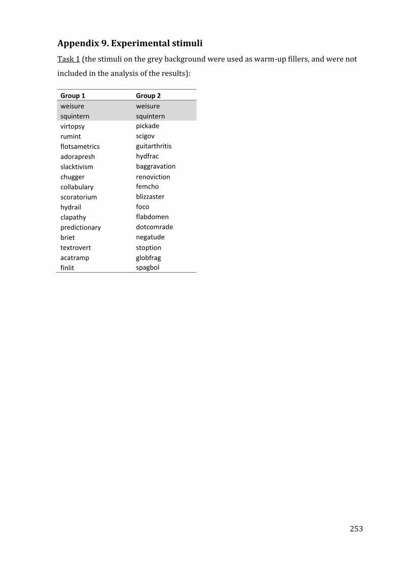
253

Appendix 9. Experimental stimuli

Task 1 (the stimuli on the grey background were used as warm-up fillers, and were not

included in the analysis of the results):

Group 1 Group 2

weisure weisure

squintern squintern

virtopsy pickade

rumint scigov

flotsametrics guitarthritis

adorapresh hydfrac

slacktivism baggravation

chugger renoviction

collabulary femcho

scoratorium blizzaster

hydrail foco

clapathy flabdomen

predictionary dotcomrade

briet negatude

textrovert stoption

acatramp globfrag

finlit spagbol

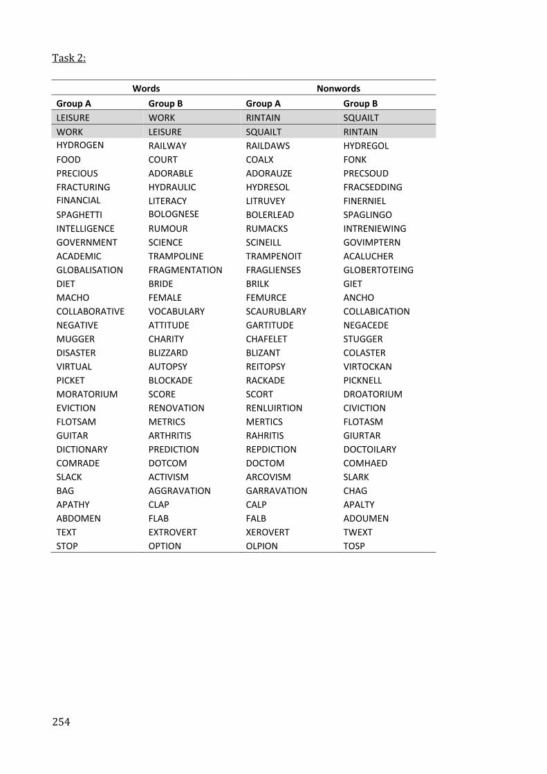
254

Task 2:

Words Nonwords

Group A Group B Group A Group B

LEISURE WORK RINTAIN SQUAILT

WORK LEISURE SQUAILT RINTAIN

HYDROGEN RAILWAY RAILDAWS HYDREGOL

FOOD COURT COALX FONK

PRECIOUS ADORABLE ADORAUZE PRECSOUD

FRACTURING HYDRAULIC HYDRESOL FRACSEDDING

FINANCIAL LITERACY LITRUVEY FINERNIEL

SPAGHETTI BOLOGNESE BOLERLEAD SPAGLINGO

INTELLIGENCE RUMOUR RUMACKS INTRENIEWING

GOVERNMENT SCIENCE SCINEILL GOVIMPTERN

ACADEMIC TRAMPOLINE TRAMPENOIT ACALUCHER

GLOBALISATION FRAGMENTATION FRAGLIENSES GLOBERTOTEING

DIET BRIDE BRILK GIET

MACHO FEMALE FEMURCE ANCHO

COLLABORATIVE VOCABULARY SCAURUBLARY COLLABICATION

NEGATIVE ATTITUDE GARTITUDE NEGACEDE

MUGGER CHARITY CHAFELET STUGGER

DISASTER BLIZZARD BLIZANT COLASTER

VIRTUAL AUTOPSY REITOPSY VIRTOCKAN

PICKET BLOCKADE RACKADE PICKNELL

MORATORIUM SCORE SCORT DROATORIUM

EVICTION RENOVATION RENLUIRTION CIVICTION

FLOTSAM METRICS MERTICS FLOTASM

GUITAR ARTHRITIS RAHRITIS GIURTAR

DICTIONARY PREDICTION REPDICTION DOCTOILARY

COMRADE DOTCOM DOCTOM COMHAED

SLACK ACTIVISM ARCOVISM SLARK

BAG AGGRAVATION GARRAVATION CHAG

APATHY CLAP CALP APALTY

ABDOMEN FLAB FALB ADOUMEN

TEXT EXTROVERT XEROVERT TWEXT

STOP OPTION OLPION TOSP

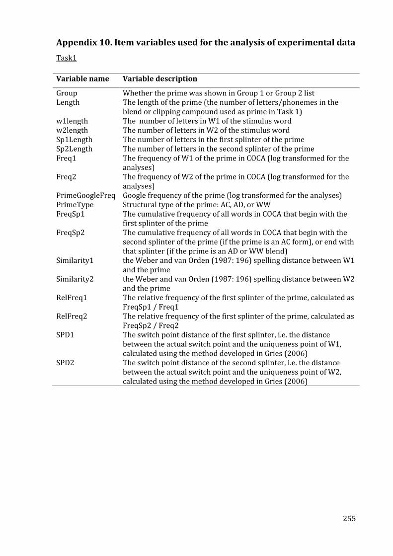
255

Appendix 10. Item variables used for the analysis of experimental data

Task1

Variable name Variable description

Group Whether the prime was shown in Group 1 or Group 2 list Length The length of the prime (the number of letters/phonemes in the

blend or clipping compound used as prime in Task 1) w1length The number of letters in W1 of the stimulus word w2length The number of letters in W2 of the stimulus word Sp1Length The number of letters in the first splinter of the prime Sp2Length The number of letters in the second splinter of the prime Freq1 The frequency of W1 of the prime in COCA (log transformed for the

analyses) Freq2 The frequency of W2 of the prime in COCA (log transformed for the

analyses) PrimeGoogleFreq Google frequency of the prime (log transformed for the analyses) PrimeType Structural type of the prime: AC, AD, or WW FreqSp1 The cumulative frequency of all words in COCA that begin with the

first splinter of the prime FreqSp2 The cumulative frequency of all words in COCA that begin with the

second splinter of the prime (if the prime is an AC form), or end with that splinter (if the prime is an AD or WW blend)

Similarity1 the Weber and van Orden (1987: 196) spelling distance between W1 and the prime

Similarity2 the Weber and van Orden (1987: 196) spelling distance between W2 and the prime

RelFreq1 The relative frequency of the first splinter of the prime, calculated as FreqSp1 / Freq1

RelFreq2 The relative frequency of the first splinter of the prime, calculated as FreqSp2 / Freq2

SPD1 The switch point distance of the first splinter, i.e. the distance between the actual switch point and the uniqueness point of W1, calculated using the method developed in Gries (2006)

SPD2 The switch point distance of the second splinter, i.e. the distance between the actual switch point and the uniqueness point of W2, calculated using the method developed in Gries (2006)

256

Task 2

Variable name Variable description PrimeShown Whether the prime for this target was shown to this group of

participants or not Tword Whether the target is a word or not Tlength The length of the target in letters LogTfreq Log-transformed COCA frequency of target PrSW Which source word of the prime is target (1 if target is the

W1 of the prime, 2 if target is the W2) Plength The length of the prime in letters LogPfreq Log-transformed Google frequency of prime PrimeType The structural type of prime (AC, AD, WW) SpLength The length of the splinter in letters (how many letters from

target are contained in prime) Similarity The Weber and van Orden spelling distance between target

and prime Pspd The switch point distance relevant for the target, i.e. the

distance between the actual switch point in the corresponding prime, and the uniqueness point of target, calculated using the method developed in Gries (2006)

Prelfreq The relative splinter frequency of the corresponding splinter of the prime, calculated by dividing the cumulative frequency of words beginning/ending with the splinter, using the method suggested in Cook and Stevenson (2007)

SimToSW The Weber and van Orden spelling distance between target and the relevant source word of prime (measured for nonword targets only)

TOrphSimilarity The proportion of the corresponding target word retained in the nonword target, calculated as the length of the letter string from target word preserved in the nonword divided by the length of the target word (measured for nonword targets only)

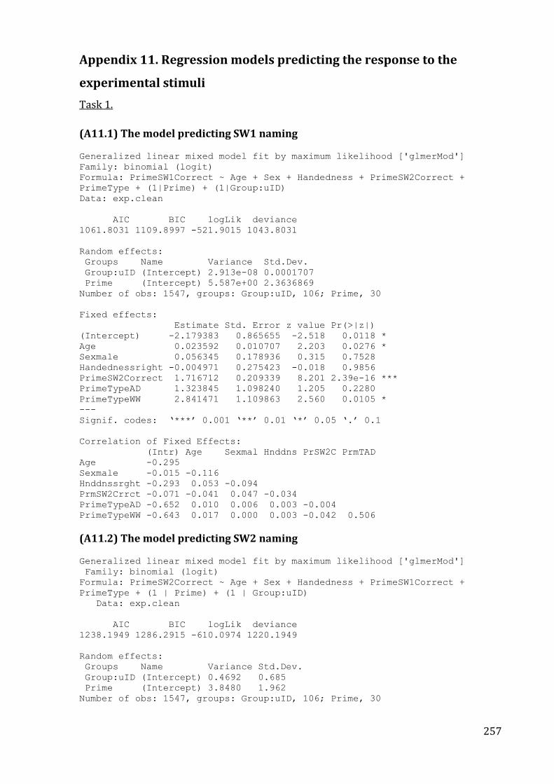
257

Appendix 11. Regression models predicting the response to the

experimental stimuli

Task 1.

(A11.1) The model predicting SW1 naming

Generalized linear mixed model fit by maximum likelihood ['glmerMod']

Family: binomial (logit)

Formula: PrimeSW1Correct ~ Age + Sex + Handedness + PrimeSW2Correct +

PrimeType + (1|Prime) + (1|Group:uID)

Data: exp.clean


1061.8031 1109.8997 -521.9015 1043.8031

Random effects:


Group:uID (Intercept) 2.913e-08 0.0001707

Prime (Intercept) 5.587e+00 2.3636869

Number of obs: 1547, groups: Group:uID, 106; Prime, 30

Fixed effects:

Estimate Std. Error z value Pr(>|z|)

(Intercept) -2.179383 0.865655 -2.518 0.0118 *

Age 0.023592 0.010707 2.203 0.0276 *

Sexmale 0.056345 0.178936 0.315 0.7528

Handednessright -0.004971 0.275423 -0.018 0.9856

PrimeSW2Correct 1.716712 0.209339 8.201 2.39e-16 ***

PrimeTypeAD 1.323845 1.098240 1.205 0.2280

PrimeTypeWW 2.841471 1.109863 2.560 0.0105 *

---

Signif. codes: ‘***’ 0.001 ‘**’ 0.01 ‘*’ 0.05 ‘.’ 0.1


(Intr) Age Sexmal Hnddns PrSW2C PrmTAD

Age -0.295

Sexmale -0.015 -0.116

Hnddnssrght -0.293 0.053 -0.094

PrmSW2Crrct -0.071 -0.041 0.047 -0.034

PrimeTypeAD -0.652 0.010 0.006 0.003 -0.004

PrimeTypeWW -0.643 0.017 0.000 0.003 -0.042 0.506

(A11.2) The model predicting SW2 naming




PrimeType + (1 | Prime) + (1 | Group:uID)

Data: exp.clean


1238.1949 1286.2915 -610.0974 1220.1949

Random effects:


Group:uID (Intercept) 0.4692 0.685

Prime (Intercept) 3.8480 1.962


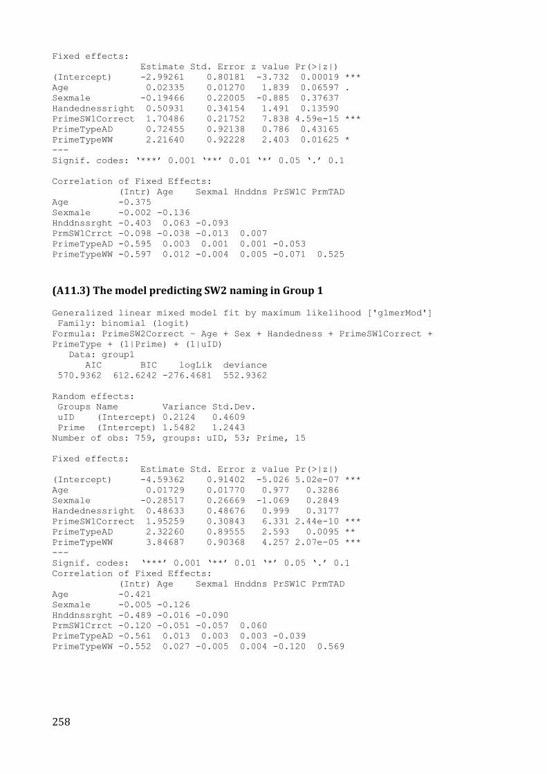
258

Fixed effects:


(Intercept) -2.99261 0.80181 -3.732 0.00019 ***

Age 0.02335 0.01270 1.839 0.06597 .

Sexmale -0.19466 0.22005 -0.885 0.37637

Handednessright 0.50931 0.34154 1.491 0.13590


PrimeTypeAD 0.72455 0.92138 0.786 0.43165

PrimeTypeWW 2.21640 0.92228 2.403 0.01625 *

---

Signif. codes: ‘***’ 0.001 ‘**’ 0.01 ‘*’ 0.05 ‘.’ 0.1



Age -0.375

Sexmale -0.002 -0.136

Hnddnssrght -0.403 0.063 -0.093

PrmSW1Crrct -0.098 -0.038 -0.013 0.007

PrimeTypeAD -0.595 0.003 0.001 0.001 -0.053

PrimeTypeWW -0.597 0.012 -0.004 0.005 -0.071 0.525

(A11.3) The model predicting SW2 naming in Group 1




PrimeType + (1|Prime) + (1|uID)

Data: group1


570.9362 612.6242 -276.4681 552.9362

Random effects:




Number of obs: 759, groups: uID, 53; Prime, 15

Fixed effects:


(Intercept) -4.59362 0.91402 -5.026 5.02e-07 ***

Age 0.01729 0.01770 0.977 0.3286

Sexmale -0.28517 0.26669 -1.069 0.2849



PrimeTypeAD 2.32260 0.89555 2.593 0.0095 **

PrimeTypeWW 3.84687 0.90368 4.257 2.07e-05 ***

---

Signif. codes: ‘***’ 0.001 ‘**’ 0.01 ‘*’ 0.05 ‘.’ 0.1



Age -0.421

Sexmale -0.005 -0.126

Hnddnssrght -0.489 -0.016 -0.090

PrmSW1Crrct -0.120 -0.051 -0.057 0.060

PrimeTypeAD -0.561 0.013 0.003 0.003 -0.039

PrimeTypeWW -0.552 0.027 -0.005 0.004 -0.120 0.569

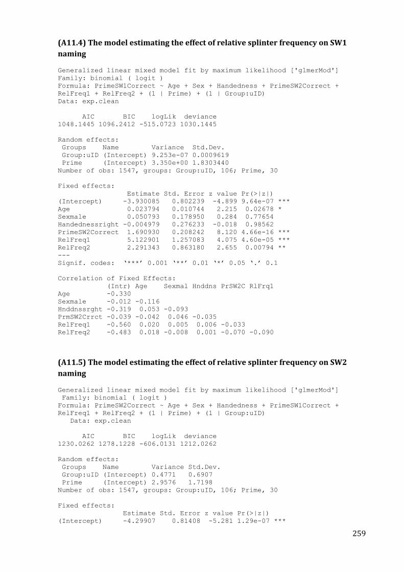
259

(A11.4) The model estimating the effect of relative splinter frequency on SW1

naming


Family: binomial ( logit )


RelFreq1 + RelFreq2 + (1 | Prime) + (1 | Group:uID)

Data: exp.clean


1048.1445 1096.2412 -515.0723 1030.1445

Random effects:





Fixed effects:


(Intercept) -3.930085 0.802239 -4.899 9.64e-07 ***

Age 0.023794 0.010744 2.215 0.02678 *

Sexmale 0.050793 0.178950 0.284 0.77654



RelFreq1 5.122901 1.257083 4.075 4.60e-05 ***

RelFreq2 2.291343 0.863180 2.655 0.00794 **

---

Signif. codes: ‘***’ 0.001 ‘**’ 0.01 ‘*’ 0.05 ‘.’ 0.1


(Intr) Age Sexmal Hnddns PrSW2C RlFrq1

Age -0.330

Sexmale -0.012 -0.116

Hnddnssrght -0.319 0.053 -0.093

PrmSW2Crrct -0.039 -0.042 0.046 -0.035

RelFreq1 -0.560 0.020 0.005 0.006 -0.033

RelFreq2 -0.483 0.018 -0.008 0.001 -0.070 -0.090

(A11.5) The model estimating the effect of relative splinter frequency on SW2

naming




RelFreq1 + RelFreq2 + (1 | Prime) + (1 | Group:uID)

Data: exp.clean


1230.0262 1278.1228 -606.0131 1212.0262

Random effects:





Fixed effects:


(Intercept) -4.29907 0.81408 -5.281 1.29e-07 ***

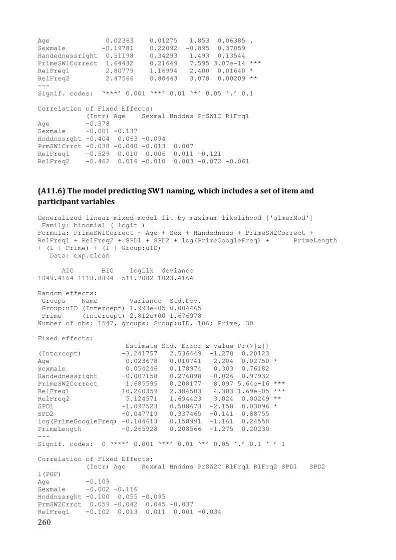
260

Age 0.02363 0.01275 1.853 0.06385 .

Sexmale -0.19781 0.22092 -0.895 0.37059



RelFreq1 2.80779 1.16994 2.400 0.01640 *

RelFreq2 2.47566 0.80443 3.078 0.00209 **

---

Signif. codes: ‘***’ 0.001 ‘**’ 0.01 ‘*’ 0.05 ‘.’ 0.1


(Intr) Age Sexmal Hnddns PrSW1C RlFrq1

Age -0.378

Sexmale -0.001 -0.137

Hnddnssrght -0.404 0.063 -0.094

PrmSW1Crrct -0.038 -0.040 -0.013 0.007

RelFreq1 -0.529 0.010 0.006 0.011 -0.121

RelFreq2 -0.462 0.016 -0.010 0.003 -0.072 -0.061

(A11.6) The model predicting SW1 naming, which includes a set of item and

participant variables




RelFreq1 + RelFreq2 + SPD1 + SPD2 + log(PrimeGoogleFreq) + PrimeLength

+ (1 | Prime) + (1 | Group:uID)

Data: exp.clean


1049.4164 1118.8894 -511.7082 1023.4164

Random effects:





Fixed effects:


(Intercept) -3.241757 2.536449 -1.278 0.20123

Age 0.023678 0.010741 2.204 0.02750 *

Sexmale 0.054246 0.178974 0.303 0.76182



RelFreq1 10.260359 2.384503 4.303 1.69e-05 ***

RelFreq2 5.124571 1.694423 3.024 0.00249 **

SPD1 -1.097523 0.508673 -2.158 0.03096 *

SPD2 -0.047719 0.337465 -0.141 0.88755

log(PrimeGoogleFreq) -0.184613 0.158991 -1.161 0.24558

PrimeLength -0.265928 0.208566 -1.275 0.20230

---

Signif. codes: 0 ‘***’ 0.001 ‘**’ 0.01 ‘*’ 0.05 ‘.’ 0.1 ‘ ’ 1


(Intr) Age Sexmal Hnddns PrSW2C RlFrq1 RlFrq2 SPD1 SPD2

l(PGF)

Age -0.109

Sexmale -0.002 -0.116

Hnddnssrght -0.100 0.055 -0.095

PrmSW2Crrct 0.059 -0.042 0.045 -0.037

RelFreq1 -0.102 0.013 0.011 0.001 -0.034

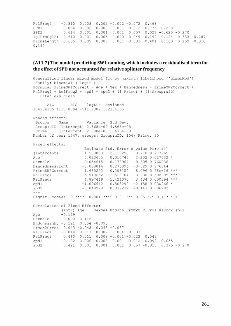
261

RelFreq2 -0.310 0.008 0.002 -0.002 -0.072 0.463

SPD1 0.054 -0.006 -0.008 0.001 0.012 -0.775 -0.298

SPD2 0.614 0.001 0.001 0.001 0.057 0.027 -0.625 -0.270

lg(PrmGglF) -0.610 0.001 -0.003 0.000 -0.049 -0.199 -0.124 0.333 -0.287

PrimeLength -0.635 0.005 -0.007 0.001 -0.033 -0.401 -0.180 0.159 -0.310

0.190

(A11.7) The model predicting SW1 naming, which includes a residualised term for

the effect of SPD not accounted for relative splinter frequency




RelFreq1 + RelFreq2 + spd1 + spd2 + (1|Prime) + (1|Group:uID)

Data: exp.clean


1049.4165 1118.8894 -511.7082 1023.4165

Random effects:


Group:uID (Intercept) 2.368e-09 4.866e-05

Prime (Intercept) 2.808e+00 1.676e+00


Fixed effects:


(Intercept) -1.503803 2.119290 -0.710 0.477965

Age 0.023655 0.010740 2.202 0.027632 *

Sexmale 0.054615 0.178964 0.305 0.760236



RelFreq1 5.948652 1.513704 3.930 8.50e-05 ***

RelFreq2 4.897469 1.426070 3.434 0.000594 ***

spd1 -1.096642 0.508292 -2.158 0.030966 *

spd2 -0.048228 0.337232 -0.143 0.886282

---

Signif. codes: 0 ‘***’ 0.001 ‘**’ 0.01 ‘*’ 0.05 ‘.’ 0.1 ‘ ’ 1


(Intr) Age Sexmal Hnddns PrSW2C RlFrq1 RlFrq2 spd1

Age -0.129

Sexmale 0.000 -0.116

Hnddnssrght -0.121 0.054 -0.095

PrmSW2Crrct 0.043 -0.043 0.045 -0.037

RelFreq1 -0.014 0.013 0.007 0.004 -0.037

RelFreq2 0.460 0.011 0.003 -0.001 -0.022 0.049

spd1 -0.182 -0.006 -0.008 0.001 0.012 0.099 -0.655

spd2 0.421 0.001 0.001 0.001 0.057 -0.313 0.375 -0.270

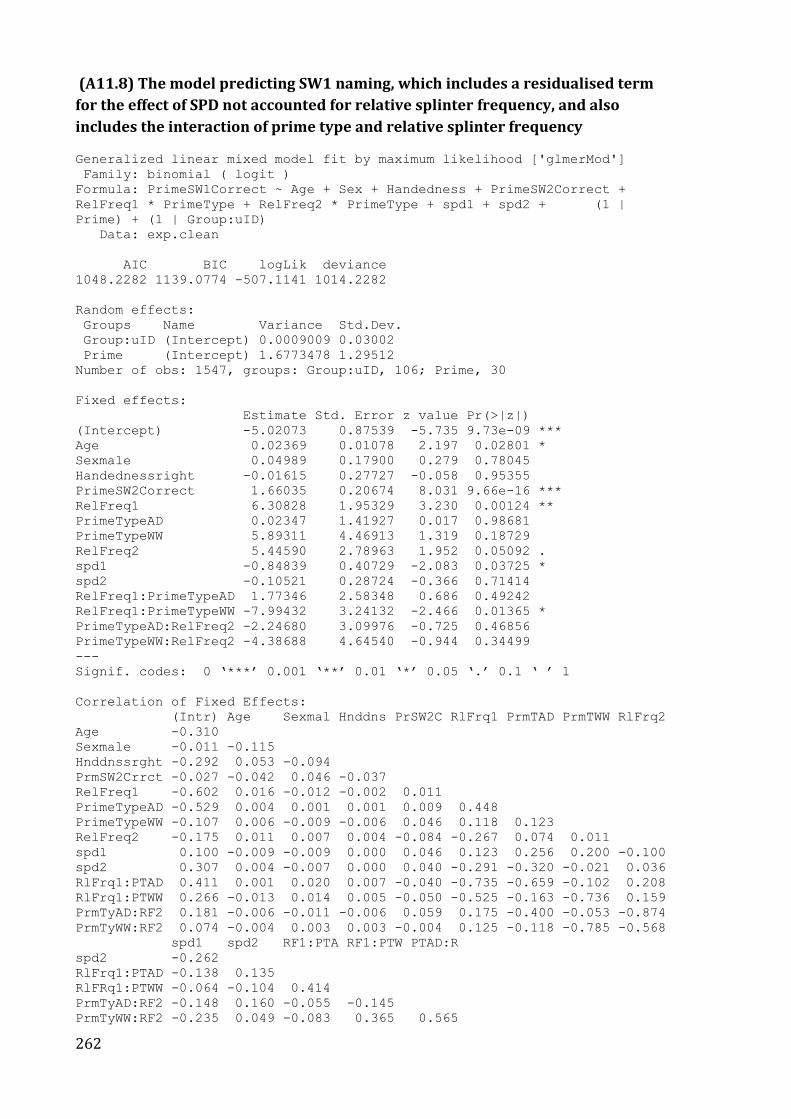
262

(A11.8) The model predicting SW1 naming, which includes a residualised term

for the effect of SPD not accounted for relative splinter frequency, and also

includes the interaction of prime type and relative splinter frequency




RelFreq1 * PrimeType + RelFreq2 * PrimeType + spd1 + spd2 + (1 |

Prime) + (1 | Group:uID)

Data: exp.clean


1048.2282 1139.0774 -507.1141 1014.2282

Random effects:





Fixed effects:


(Intercept) -5.02073 0.87539 -5.735 9.73e-09 ***

Age 0.02369 0.01078 2.197 0.02801 *

Sexmale 0.04989 0.17900 0.279 0.78045



RelFreq1 6.30828 1.95329 3.230 0.00124 **

PrimeTypeAD 0.02347 1.41927 0.017 0.98681

PrimeTypeWW 5.89311 4.46913 1.319 0.18729

RelFreq2 5.44590 2.78963 1.952 0.05092 .

spd1 -0.84839 0.40729 -2.083 0.03725 *

spd2 -0.10521 0.28724 -0.366 0.71414

RelFreq1:PrimeTypeAD 1.77346 2.58348 0.686 0.49242

RelFreq1:PrimeTypeWW -7.99432 3.24132 -2.466 0.01365 *

PrimeTypeAD:RelFreq2 -2.24680 3.09976 -0.725 0.46856

PrimeTypeWW:RelFreq2 -4.38688 4.64540 -0.944 0.34499

---

Signif. codes: 0 ‘***’ 0.001 ‘**’ 0.01 ‘*’ 0.05 ‘.’ 0.1 ‘ ’ 1


(Intr) Age Sexmal Hnddns PrSW2C RlFrq1 PrmTAD PrmTWW RlFrq2

Age -0.310

Sexmale -0.011 -0.115

Hnddnssrght -0.292 0.053 -0.094

PrmSW2Crrct -0.027 -0.042 0.046 -0.037

RelFreq1 -0.602 0.016 -0.012 -0.002 0.011

PrimeTypeAD -0.529 0.004 0.001 0.001 0.009 0.448

PrimeTypeWW -0.107 0.006 -0.009 -0.006 0.046 0.118 0.123

RelFreq2 -0.175 0.011 0.007 0.004 -0.084 -0.267 0.074 0.011

spd1 0.100 -0.009 -0.009 0.000 0.046 0.123 0.256 0.200 -0.100

spd2 0.307 0.004 -0.007 0.000 0.040 -0.291 -0.320 -0.021 0.036

RlFrq1:PTAD 0.411 0.001 0.020 0.007 -0.040 -0.735 -0.659 -0.102 0.208

RlFrq1:PTWW 0.266 -0.013 0.014 0.005 -0.050 -0.525 -0.163 -0.736 0.159

PrmTyAD:RF2 0.181 -0.006 -0.011 -0.006 0.059 0.175 -0.400 -0.053 -0.874

PrmTyWW:RF2 0.074 -0.004 0.003 0.003 -0.004 0.125 -0.118 -0.785 -0.568

spd1 spd2 RF1:PTA RF1:PTW PTAD:R

spd2 -0.262

RlFrq1:PTAD -0.138 0.135

RlFRq1:PTWW -0.064 -0.104 0.414

PrmTyAD:RF2 -0.148 0.160 -0.055 -0.145

PrmTyWW:RF2 -0.235 0.049 -0.083 0.365 0.565

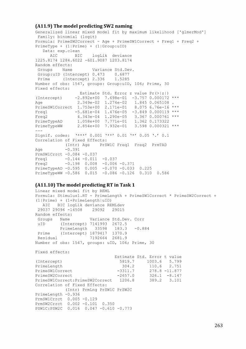
263

(A11.9) The model predicting SW2 naming Generalized linear mixed model fit by maximum likelihood ['glmerMod']


Formula: PrimeSW2Correct ~ Age + PrimeSW1Correct + Freq1 + Freq2 +

PrimeType + (1|Prime) + (1|Group:uID)

Data: exp.clean


1225.8174 1284.6022 -601.9087 1203.8174

Random effects:





Fixed effects:


(Intercept) -2.892e+00 7.698e-01 -3.757 0.000172 ***

Age 2.349e-02 1.274e-02 1.845 0.065108 .

PrimeSW1Correct 1.753e+00 2.171e-01 8.075 6.76e-16 ***

Freq1 -5.681e-04 1.476e-05 -3.849 0.000119 ***

Freq2 4.343e-04 1.290e-05 3.367 0.000761 ***

PrimeTypeAD 1.058e+00 7.771e-01 1.362 0.173322

PrimeTypeWW 2.854e+00 7.932e-01 3.598 0.000321 ***

---

Signif. codes: ‘***’ 0.001 ‘**’ 0.01 ‘*’ 0.05 ‘.’ 0.1


(Intr) Age PrSW1C Freq1 Freq2 PrmTAD

Age -0.391

PrmSW1Crrct -0.084 -0.037

Freq1 -0.144 -0.011 -0.037

Freq2 -0.198 0.008 -0.006 -0.371

PrimeTypeAD -0.595 0.005 -0.070 -0.033 0.225

PrimeTypeWW -0.586 0.015 -0.086 -0.126 0.310 0.586

(A11.10) The model predicting RT in Task 1 Linear mixed model fit by REML

Formula: Stimulus1.RT ~ PrimeLength + PrimeSW1Correct * PrimeSW2Correct +

(1|Prime) + (1+PrimeLength|uID)

AIC BIC logLik deviance REMLdev

29037 29096 -14508 29092 29015

Random effects:


uID (Intercept) 7141993 2672.5

PrimeLength 33598 183.3 -0.884

Prime (Intercept) 1879417 1370.9

Residual 7192664 2681.9

Number of obs: 1547, groups: uID, 106; Prime, 30

Fixed effects:


(Intercept) 5819.7 1003.6 5.799

PrimeLength 304.2 110.6 2.751

PrimeSW1Correct -3311.7 278.8 -11.877

PrimeSW2Correct -2657.0 326.1 -8.147

PrimeSW1Correct:PrimeSW2Correct 1206.8 389.2 3.101


(Intr) PrmLng PrSW1C PrSW2C

PrimeLength -0.936

PrmSW1Crrct 0.005 -0.129

PrmSW2Crrct 0.002 -0.101 0.350

PSW1C:PSW2C 0.016 0.047 -0.610 -0.773

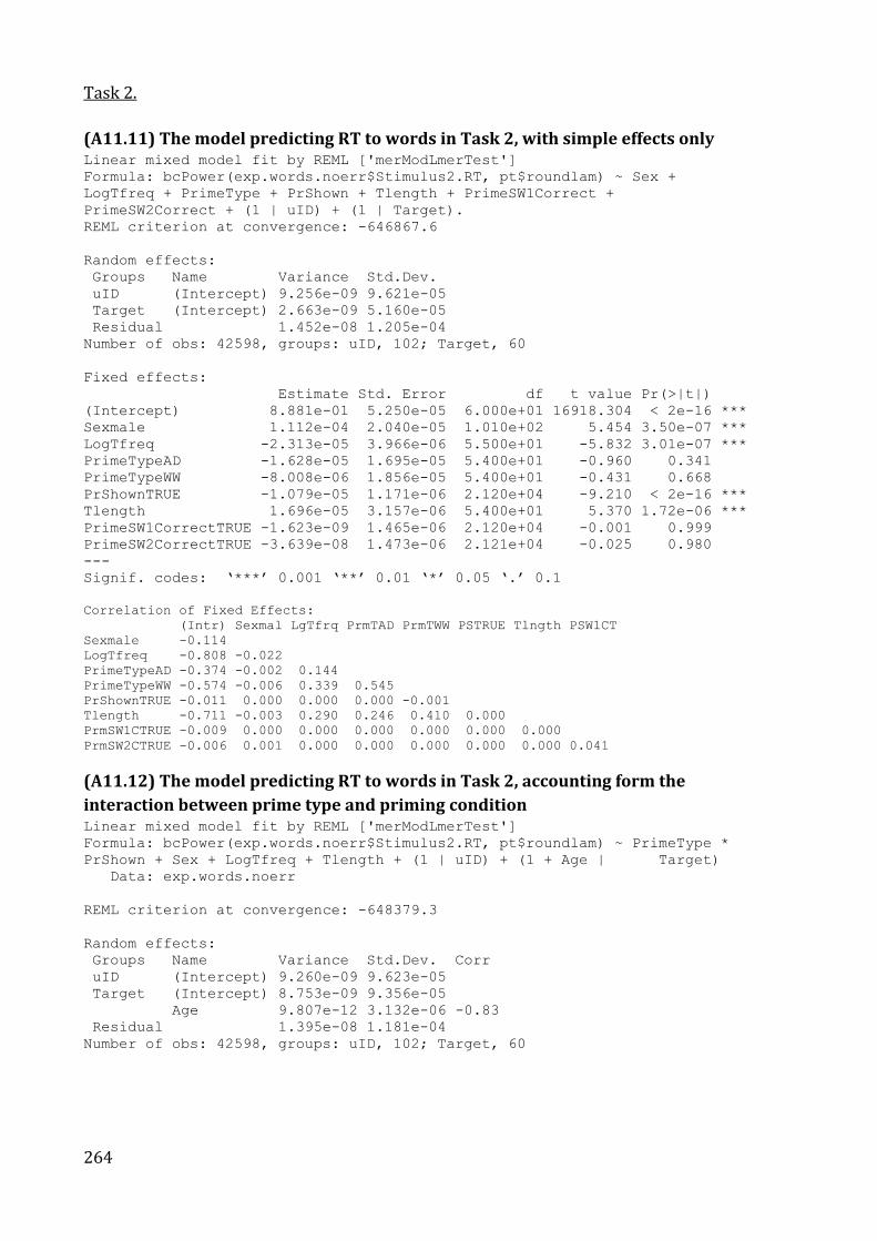
264

Task 2.

(A11.11) The model predicting RT to words in Task 2, with simple effects only Linear mixed model fit by REML ['merModLmerTest']

Formula: bcPower(exp.words.noerr$Stimulus2.RT, pt$roundlam) ~ Sex +

LogTfreq + PrimeType + PrShown + Tlength + PrimeSW1Correct +

PrimeSW2Correct + (1 | uID) + (1 | Target).

REML criterion at convergence: -646867.6

Random effects:


uID (Intercept) 9.256e-09 9.621e-05

Target (Intercept) 2.663e-09 5.160e-05

Residual 1.452e-08 1.205e-04

Number of obs: 42598, groups: uID, 102; Target, 60

Fixed effects:

Estimate Std. Error df t value Pr(>|t|)

(Intercept) 8.881e-01 5.250e-05 6.000e+01 16918.304 < 2e-16 ***

Sexmale 1.112e-04 2.040e-05 1.010e+02 5.454 3.50e-07 ***

LogTfreq -2.313e-05 3.966e-06 5.500e+01 -5.832 3.01e-07 ***

PrimeTypeAD -1.628e-05 1.695e-05 5.400e+01 -0.960 0.341

PrimeTypeWW -8.008e-06 1.856e-05 5.400e+01 -0.431 0.668

PrShownTRUE -1.079e-05 1.171e-06 2.120e+04 -9.210 < 2e-16 ***

Tlength 1.696e-05 3.157e-06 5.400e+01 5.370 1.72e-06 ***

PrimeSW1CorrectTRUE -1.623e-09 1.465e-06 2.120e+04 -0.001 0.999

PrimeSW2CorrectTRUE -3.639e-08 1.473e-06 2.121e+04 -0.025 0.980

---

Signif. codes: ‘***’ 0.001 ‘**’ 0.01 ‘*’ 0.05 ‘.’ 0.1


(Intr) Sexmal LgTfrq PrmTAD PrmTWW PSTRUE Tlngth PSW1CT

Sexmale -0.114

LogTfreq -0.808 -0.022

PrimeTypeAD -0.374 -0.002 0.144

PrimeTypeWW -0.574 -0.006 0.339 0.545

PrShownTRUE -0.011 0.000 0.000 0.000 -0.001

Tlength -0.711 -0.003 0.290 0.246 0.410 0.000

PrmSW1CTRUE -0.009 0.000 0.000 0.000 0.000 0.000 0.000

PrmSW2CTRUE -0.006 0.001 0.000 0.000 0.000 0.000 0.000 0.041

(A11.12) The model predicting RT to words in Task 2, accounting form the

interaction between prime type and priming condition Linear mixed model fit by REML ['merModLmerTest']

Formula: bcPower(exp.words.noerr$Stimulus2.RT, pt$roundlam) ~ PrimeType *

PrShown + Sex + LogTfreq + Tlength + (1 | uID) + (1 + Age | Target)

Data: exp.words.noerr


Random effects:




Age 9.807e-12 3.132e-06 -0.83

Residual 1.395e-08 1.181e-04


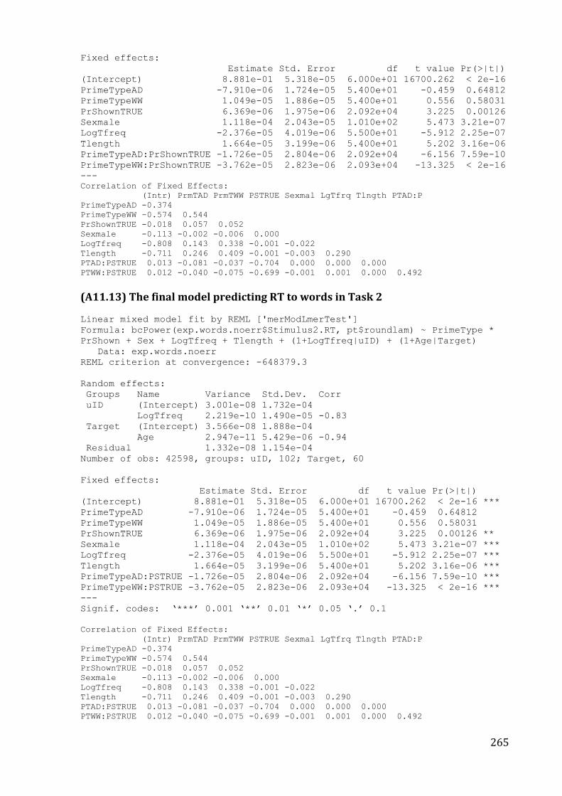
265

Fixed effects:


(Intercept) 8.881e-01 5.318e-05 6.000e+01 16700.262 < 2e-16

PrimeTypeAD -7.910e-06 1.724e-05 5.400e+01 -0.459 0.64812

PrimeTypeWW 1.049e-05 1.886e-05 5.400e+01 0.556 0.58031

PrShownTRUE 6.369e-06 1.975e-06 2.092e+04 3.225 0.00126

Sexmale 1.118e-04 2.043e-05 1.010e+02 5.473 3.21e-07

LogTfreq -2.376e-05 4.019e-06 5.500e+01 -5.912 2.25e-07

Tlength 1.664e-05 3.199e-06 5.400e+01 5.202 3.16e-06

PrimeTypeAD:PrShownTRUE -1.726e-05 2.804e-06 2.092e+04 -6.156 7.59e-10

PrimeTypeWW:PrShownTRUE -3.762e-05 2.823e-06 2.093e+04 -13.325 < 2e-16

---


(Intr) PrmTAD PrmTWW PSTRUE Sexmal LgTfrq Tlngth PTAD:P

PrimeTypeAD -0.374

PrimeTypeWW -0.574 0.544

PrShownTRUE -0.018 0.057 0.052

Sexmale -0.113 -0.002 -0.006 0.000

LogTfreq -0.808 0.143 0.338 -0.001 -0.022

Tlength -0.711 0.246 0.409 -0.001 -0.003 0.290

PTAD:PSTRUE 0.013 -0.081 -0.037 -0.704 0.000 0.000 0.000

PTWW:PSTRUE 0.012 -0.040 -0.075 -0.699 -0.001 0.001 0.000 0.492

(A11.13) The final model predicting RT to words in Task 2

Linear mixed model fit by REML ['merModLmerTest']

Formula: bcPower(exp.words.noerr$Stimulus2.RT, pt$roundlam) ~ PrimeType *

PrShown + Sex + LogTfreq + Tlength + (1+LogTfreq|uID) + (1+Age|Target)

Data: exp.words.noerr


Random effects:



LogTfreq 2.219e-10 1.490e-05 -0.83


Age 2.947e-11 5.429e-06 -0.94

Residual 1.332e-08 1.154e-04


Fixed effects:


(Intercept) 8.881e-01 5.318e-05 6.000e+01 16700.262 < 2e-16 ***

PrimeTypeAD -7.910e-06 1.724e-05 5.400e+01 -0.459 0.64812

PrimeTypeWW 1.049e-05 1.886e-05 5.400e+01 0.556 0.58031

PrShownTRUE 6.369e-06 1.975e-06 2.092e+04 3.225 0.00126 **

Sexmale 1.118e-04 2.043e-05 1.010e+02 5.473 3.21e-07 ***

LogTfreq -2.376e-05 4.019e-06 5.500e+01 -5.912 2.25e-07 ***

Tlength 1.664e-05 3.199e-06 5.400e+01 5.202 3.16e-06 ***

PrimeTypeAD:PSTRUE -1.726e-05 2.804e-06 2.092e+04 -6.156 7.59e-10 ***

PrimeTypeWW:PSTRUE -3.762e-05 2.823e-06 2.093e+04 -13.325 < 2e-16 ***

---

Signif. codes: ‘***’ 0.001 ‘**’ 0.01 ‘*’ 0.05 ‘.’ 0.1


(Intr) PrmTAD PrmTWW PSTRUE Sexmal LgTfrq Tlngth PTAD:P

PrimeTypeAD -0.374

PrimeTypeWW -0.574 0.544

PrShownTRUE -0.018 0.057 0.052

Sexmale -0.113 -0.002 -0.006 0.000

LogTfreq -0.808 0.143 0.338 -0.001 -0.022

Tlength -0.711 0.246 0.409 -0.001 -0.003 0.290

PTAD:PSTRUE 0.013 -0.081 -0.037 -0.704 0.000 0.000 0.000

PTWW:PSTRUE 0.012 -0.040 -0.075 -0.699 -0.001 0.001 0.000 0.492

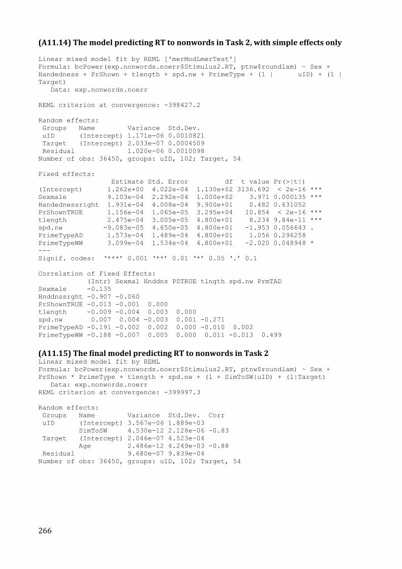
266

(A11.14) The model predicting RT to nonwords in Task 2, with simple effects only

Linear mixed model fit by REML ['merModLmerTest']

Formula: bcPower(exp.nonwords.noerr$Stimulus2.RT, ptnw$roundlam) ~ Sex +

Handedness + PrShown + tlength + spd.nw + PrimeType + (1 | uID) + (1 |

Target)

Data: exp.nonwords.noerr


Random effects:


uID (Intercept) 1.171e-06 0.0010821

Target (Intercept) 2.033e-07 0.0004509

Residual 1.020e-06 0.0010098


Fixed effects:


(Intercept) 1.262e+00 4.022e-04 1.130e+02 3136.692 < 2e-16 ***

Sexmale 9.103e-04 2.292e-04 1.000e+02 3.971 0.000135 ***

Handednessright 1.931e-04 4.008e-04 9.900e+01 0.482 0.631052

PrShownTRUE 1.156e-04 1.065e-05 3.295e+04 10.854 < 2e-16 ***

tlength 2.475e-04 3.005e-05 4.800e+01 8.234 9.84e-11 ***

spd.nw -9.083e-05 4.650e-05 4.800e+01 -1.953 0.056643 .

PrimeTypeAD 1.573e-04 1.489e-04 4.800e+01 1.056 0.296258

PrimeTypeWW 3.099e-04 1.534e-04 4.800e+01 -2.020 0.048948 *

---

Signif. codes: ‘***’ 0.001 ‘**’ 0.01 ‘*’ 0.05 ‘.’ 0.1


(Intr) Sexmal Hnddns PSTRUE tlngth spd.nw PrmTAD

Sexmale -0.135

Hnddnssrght -0.907 -0.060

PrShownTRUE -0.013 -0.001 0.000

tlength -0.009 -0.004 0.003 0.000

spd.nw 0.007 0.004 -0.003 0.001 -0.271

PrimeTypeAD -0.191 -0.002 0.002 0.000 -0.010 0.002

PrimeTypeWW -0.188 -0.007 0.005 0.000 0.011 -0.013 0.499

(A11.15) The final model predicting RT to nonwords in Task 2 Linear mixed model fit by REML

Formula: bcPower(exp.nonwords.noerr$Stimulus2.RT, ptnw$roundlam) ~ Sex +

PrShown * PrimeType + tlength + spd.nw + (1 + SimToSW|uID) + (1|Target)

Data: exp.nonwords.noerr


Random effects:



SimToSW 4.530e-12 2.128e-06 -0.83


Age 2.486e-12 4.249e-03 -0.88

Residual 9.680e-07 9.839e-04


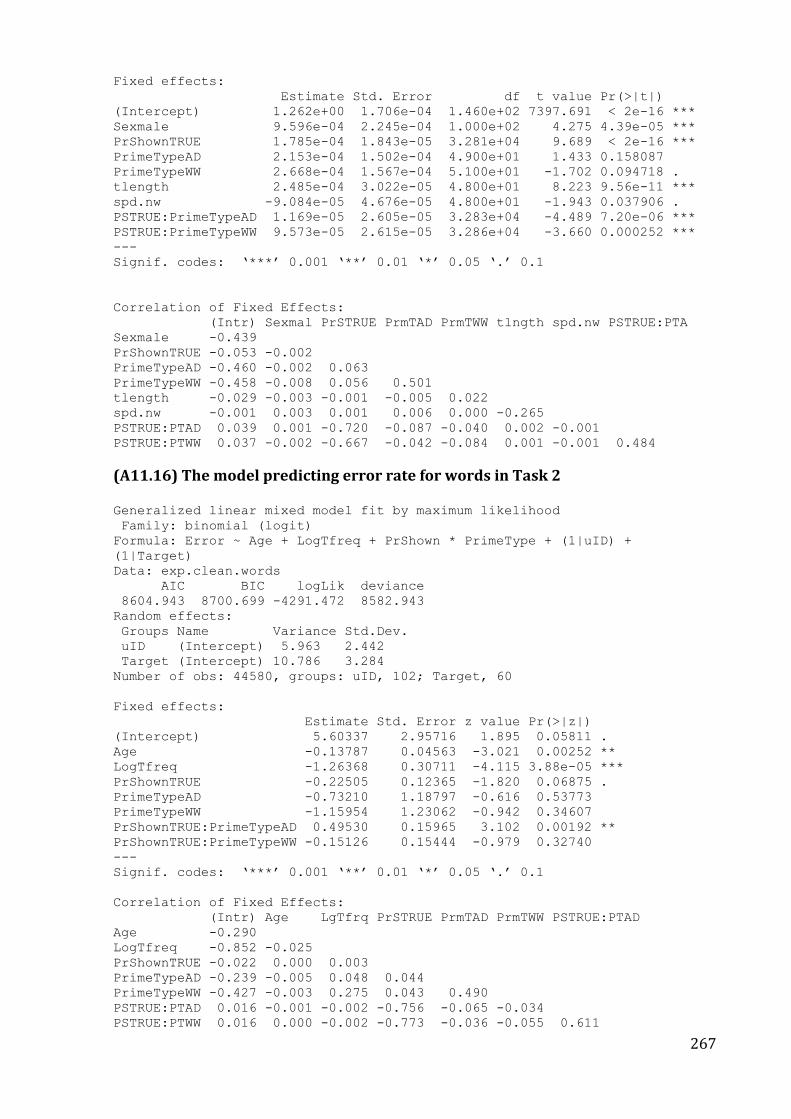
267

Fixed effects:


(Intercept) 1.262e+00 1.706e-04 1.460e+02 7397.691 < 2e-16 ***

Sexmale 9.596e-04 2.245e-04 1.000e+02 4.275 4.39e-05 ***

PrShownTRUE 1.785e-04 1.843e-05 3.281e+04 9.689 < 2e-16 ***

PrimeTypeAD 2.153e-04 1.502e-04 4.900e+01 1.433 0.158087

PrimeTypeWW 2.668e-04 1.567e-04 5.100e+01 -1.702 0.094718 .

tlength 2.485e-04 3.022e-05 4.800e+01 8.223 9.56e-11 ***

spd.nw -9.084e-05 4.676e-05 4.800e+01 -1.943 0.037906 .

PSTRUE:PrimeTypeAD 1.169e-05 2.605e-05 3.283e+04 -4.489 7.20e-06 ***

PSTRUE:PrimeTypeWW 9.573e-05 2.615e-05 3.286e+04 -3.660 0.000252 ***

---

Signif. codes: ‘***’ 0.001 ‘**’ 0.01 ‘*’ 0.05 ‘.’ 0.1


(Intr) Sexmal PrSTRUE PrmTAD PrmTWW tlngth spd.nw PSTRUE:PTA

Sexmale -0.439

PrShownTRUE -0.053 -0.002

PrimeTypeAD -0.460 -0.002 0.063

PrimeTypeWW -0.458 -0.008 0.056 0.501

tlength -0.029 -0.003 -0.001 -0.005 0.022

spd.nw -0.001 0.003 0.001 0.006 0.000 -0.265

PSTRUE:PTAD 0.039 0.001 -0.720 -0.087 -0.040 0.002 -0.001

PSTRUE:PTWW 0.037 -0.002 -0.667 -0.042 -0.084 0.001 -0.001 0.484

(A11.16) The model predicting error rate for words in Task 2 Generalized linear mixed model fit by maximum likelihood


Formula: Error ~ Age + LogTfreq + PrShown * PrimeType + (1|uID) +

(1|Target)

Data: exp.clean.words


8604.943 8700.699 -4291.472 8582.943

Random effects:



Target (Intercept) 10.786 3.284


Fixed effects:


(Intercept) 5.60337 2.95716 1.895 0.05811 .

Age -0.13787 0.04563 -3.021 0.00252 **

LogTfreq -1.26368 0.30711 -4.115 3.88e-05 ***

PrShownTRUE -0.22505 0.12365 -1.820 0.06875 .

PrimeTypeAD -0.73210 1.18797 -0.616 0.53773

PrimeTypeWW -1.15954 1.23062 -0.942 0.34607

PrShownTRUE:PrimeTypeAD 0.49530 0.15965 3.102 0.00192 **

PrShownTRUE:PrimeTypeWW -0.15126 0.15444 -0.979 0.32740

---

Signif. codes: ‘***’ 0.001 ‘**’ 0.01 ‘*’ 0.05 ‘.’ 0.1


(Intr) Age LgTfrq PrSTRUE PrmTAD PrmTWW PSTRUE:PTAD

Age -0.290

LogTfreq -0.852 -0.025

PrShownTRUE -0.022 0.000 0.003

PrimeTypeAD -0.239 -0.005 0.048 0.044

PrimeTypeWW -0.427 -0.003 0.275 0.043 0.490

PSTRUE:PTAD 0.016 -0.001 -0.002 -0.756 -0.065 -0.034

PSTRUE:PTWW 0.016 0.000 -0.002 -0.773 -0.036 -0.055 0.611

268

(A11.17) The model predicting error rate for nonwords in Task 2 Generalized linear mixed model fit by maximum likelihood


Formula: Error ~ Age + Tlength + PrShown * SimToPrime + (1|uID) +

(1|Target)

Data: exp.clean.nonwords


16175.789 16244.539 -8079.894 16159.789

Random effects:



Target (Intercept) 5.686 2.385


Fixed effects:


(Intercept) -7.2944155 1.5688987 -4.649 3.33e-06 ***

Age -0.0597923 0.0260627 -2.294 0.021781 *

Tlength 0.3428641 0.1495786 2.292 0.021894 *

PrShownTRUE -0.5218644 0.1481934 -3.522 0.000429 ***

SimToPrime 0.0028572 0.0020136 1.419 0.155926

PrShownTRUE:SimToPrime 0.0009214 0.0002682 3.435 0.000593 ***

---

Signif. codes: ‘***’ 0.001 ‘**’ 0.01 ‘*’ 0.05 ‘.’ 0.1


(Intr) Age Tlngth PrSTRUE SmTPrm

Age -0.381

Tlength -0.627 0.001

PrShownTRUE -0.045 -0.001 0.001

SimToPrime -0.502 0.006 -0.194 0.061

PrSTRUE:STP 0.043 0.000 -0.001 -0.960 -0.064

Documents

Unpacking contemporary English blends: Morphological