Understanding Evolved Genetic Programs for a Real World Object Detection Problem

Understanding Evolved Genetic Programs for aReal World Object Detection Problem

Victor Ciesielski1, Andrew Innes1, Sabu John2, and John Mamutil3

1 School of Computer Science and Information Technology,RMIT University, GPO Box 2476V, Melbourne, Vic Australia 3001

{vc, ainnes}@cs.rmit.edu.au2 School of Aerospace, Mechanical and Manufacturing Engineering,

RMIT University3 Braces Pty Ltd, 404 Windsor Road, NSW 2153, Australia

Abstract. We describe an approach to understanding evolved programsfor a real world object detection problem, that of finding orthodonticlandmarks in cranio-facial X-Rays. The approach involves modifying thefitness function to encourage the evolution of small programs, limiting thefunction set to a minimal number of operators and limiting the number ofterminals (features). When this was done for two landmarks, an easy oneand a difficult one, the evolved programs implemented a linear function ofthe features. Analysis of these linear functions revealed that underlyingregularities were being captured and that successful evolutionary runsusually terminated with the best programs implementing one of a smallnumber of underlying algorithms. Analysis of these algorithms revealedthat they are a realistic solution to the object detection problem, giventhe features and operators available.

1 Introduction

Genetic programming has been used with considerable success for a wide rangeof problems, both toy and real world. In the area of image processing therehave been a number of successful applications to difficult problems. One of thedrawbacks of genetic programming solutions is that the evolved programs arevery hard to understand and can be very big. This makes it hard to sell geneticprogramming solutions as many engineers and other professionals, particularlyin the medical area, are very unhappy with black box solutions. They want tounderstand the operation of any solution to better appreciate its limitations andgenerality.

There has been very little prior work on the problem of understanding evolvedprogram trees. Most work is focused on finding acceptable solutions to problemswithout any major concern for their understandability. However, [1] describes‘trait mining’, a method of finding sub-trees, or traits, in the evolved programs.Traits are associated with high fitness and provide some insight into the evolvedsolutions. The basic idea is that even if the whole program cannot be understood,

M. Keijzer et al. (Eds.): EuroGP 2005, LNCS 3447, pp. 351–360, 2005.c© Springer-Verlag Berlin Heidelberg 2005

352 V. Ciesielski et al.

being able to understand some of the subtrees means that the evolved programis not a black box. [2] describes the evolution of classification rules with geneticprogramming. The rules are intended to be understandable to humans. This isachieved by evolving the rules in a predetermined if-then format, rather than asfull genetic programs. [3] describes an approach to finding the underlying reg-ularities in evolved programs which use pixel inputs for texture discrimination.A strategy of limiting the function set and penalising large programs was used.Analysis of the resulting programs revealed that a number of masks of pixelpositions were being used to discriminate textures. Systematic regularities wereconsistently being discovered in the different runs, arbitrary positions of pixelswere not being used.

We have recently had considerable success in using genetic programming toevolve object detection programs for finding orthodontic landmarks in cranio-facial X-Rays [4]. Orthodontists are not comfortable with genetic programmingand there is a need to explain the evolved programs in ways that are credibleto them. The aim of the work presented in this paper is to determine whetherwe can explain how evolved programs work for the object detection problem. Inparticular we are interested in:

1. Can we develop a methodology for analysing evolved programs?2. Are regularities being discovered? If so what are they?3. Can we express, in some reasonable way, the underlying algorithms in the

evolved programs.

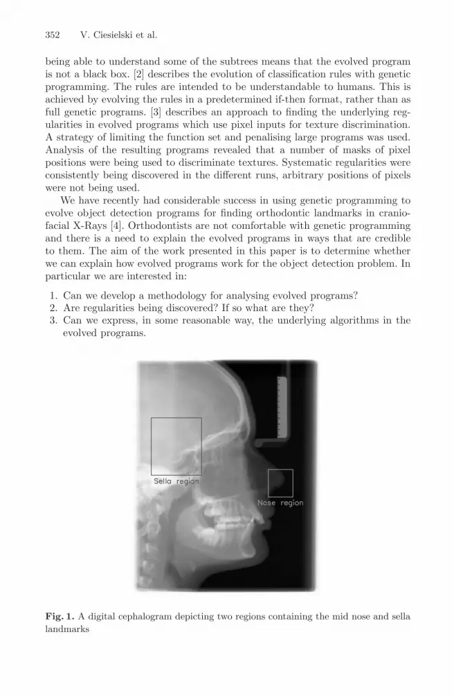
Fig. 1. A digital cephalogram depicting two regions containing the mid nose and sella

landmarks

Understanding Evolved Genetic Programs 353

square size=14

Features Local regionsµ σ

M1 S1 full square A-B-C-D

M2 S2 left half A-E-F-D

M3 S3 right half E-D-C-F

M4 S4 2 centre columns E-F

M5 S5 2 centre rows G-H

square size=40

Features Local regionsµ σ

M1 S1 shaded region

M2 S2 unshaded region

M3 S3 full square A-B-C-D

M4 S4 top left A-E-o-G

M5 S5 top right E-B-H-o

M6 S6 bottom left G-o-F-D

M7 S7 bottom right o-H-C-F

Fig. 2. The diagrams in the left column depict the feature maps used for the nose and

sella landmarks. The features consist of the mean and standard deviation calculated

for each shape from grey level intensities. The corresponding pictures in the middle

column depict the size of the feature map (shown as the white square) relative to the

image

2 The Object Detection Problem

The object detection problem is to locate, to within 2mm, a number of keylandmarks used by orthodontists in treatment planning. Full details of thisproblem can be found in [4, 5, 6]. For this paper we focus on just two land-marks, an easy one, the tip of the nose and a very difficult one, the sella.These landmarks are shown in figures 1 and 2. We consider the finding of eachlandmark as an independent object detection problem. Using prior knowledgeof facial geometry we identify regions in the picture where the landmark shouldbe with respect to the edge of the ruler which is easy to find by classical im-age processing methods. Each of these individual problems is solved indepen-dently using the method described in the next section. It might appear thatthe problem of finding the nose tip would be very straight forward, but thisis not the case due to the wide variation between humans in nose shapes andvarious noise effects on the X-Rays.


3 Finding Object Detection Programs by GeneticProgramming

The basic method is to take an input window of pixels and slide the windowover all positions in the region to find the location of the landmark [4]. Thisis similar to the template matching approach in classical vision except that thetemplate is implemented as a genetic program. The output of the program isinterpreted as the presence or absence of the landmark at the pixel position atthe centre of the window. Since we know that there can be only one landmarkin the region and that it must occur, we use the position with the largest outputas the predicted position of the object.

The evolved programs use a feature set of pixel statistics of regions, or shapes,customised for each landmark. The features are obtained from a square inputwindow centred on the landmark and large enough to contain key landmarkcharacteristics, but not large enough to introduce unnecessary clutter, as shownin figure 2. For the nose point the input window has been partitioned manuallyinto the shapes shown and the means and standard deviations of the pixels ineach shape are the features. For the sella point the input window has been seg-mented into shapes by the use of pulse coded neural networks as described in [7].The feature values are used as the terminals and the function set is {+,−,×,%}(% denotes protected division).

A data base of images marked up by an orthodontist is used in training.To evaluate fitness during training, each program is applied, in moving windowfashion, across each of the training images and the detection rate is computed.The detection rate is used as the fitness measure.

The method was tested on a number of landmark points, ranging from rel-atively easy to very difficult. Detection performance on the easier points wasexcellent and the performance on the difficult points was quite good [4].

4 Methodology for Analysing Evolved Programs

The evolved programs from the system described in the previous section are largeand difficult to understand. To evolve smaller programs which have a higherlikelihood of being understood we repeat the evolutionary process with:

1. A size penalty for large programs. The fitness function is

fitness = (1 − Dr) × 100 +Program Size

511× 1

10, (1)

where Dr is the detection rate.

Program Size is the number of nodes in the program and there are 511nodes in a full tree of depth 9, which is the max depth used in the runs.The size component represents constant parsimony pressure. The weightingsof the two terms ensures that accuracy is the primary objective and size issecondary.


2. A reduced function set. For the nose point we use the two function sets {+}and {+,−}. By keeping the operators to plus and minus we ensure that anevolved program will be a linear function of the inputs, possibly making itless accurate, but hopefully, easy to analyse.

3. A reduced terminal set. For the sella point we first use a terminal set whichcontains only the most obviously useful features together with the terminalset {+,−}. We then extend the analysis to the full terminal set.

5 Analysis of Evolved Programs

5.1 Easy Landmark: Nose

Function Set is {+}: The fittest individual, which was evolved in all 80 evolu-tionary runs, was:

Output = S5 (2)

Recalling that the position of the highest output is the predicted positionof the object, and noting from figure 2 that S5 is the standard deviation ofthe centre 2 rows of pixels, this program implements a reasonable algorithm fordetecting the nose point. Inspection of figure 2 confirms that S5 will be at amaximum when the input window is positioned over the nose tip. This programhas a detection accuracy of 65.9%. It fails on a number of images, like the lowerimage in figure 3, in which there are some edge effects near the nose. However,it appears that the methodology is producing the best program possible giventhe restricted function set.

Function Set is {+,−}: In this situation all of the evolved programs can besimplified to the form given in equation 3. All αi and βi will be integers.

Output = α1M1 + β1S1 + α2M2 + β2S2 + · · · + α5M5 + β5S5 (3)

Analysis of the best programs evolved in 80 runs revealed the following un-derlying algorithms:

Output = M1 − S2 − S3 − 2M4 + M5 (4)Output = M2 − 2S2 − 2M4 + M5 (5)Output = 2M1 − S1 − 2M4 − S4 (6)Output = M2 − 2S2 − 2M4 + M5 (7)

Analysis of an Individual Program: The following is an analysis of how the de-tection program described in equation 4 predicts the position of the landmarkbased on the values of features at six carefully chosen positions on an image.Each position used in figure 3 is indicative of regular patterns that occur in thetraining images. The window is located on soft tissue(1), the background(2),soft-tissue/background edge(3) and centred on the known position of the nose


Position Output

M1 - S2 - S3 - 2M4 + M5

1 23.3-0.9-1.3-45.8+22.3=-2.4

2 4.5-0.5-0.5- 8.6+ 4.8=-0.3

3 11.6-5.1-3.3-22.4+12.0=-7.2

4 10.2-3.9-0.3-14.2+10.8= 2.6

Highest Err =(1,-1) 9.2-4.7-0.2-10.5+ 9.8= 3.6

5 10.1-3.1-1.4-15.5+10.6= 0.7

6 6.8-1.3-2.7-11.0+ 6.7=-1.5

Highest Err =(1,0) 9.5-3.9-1.8-10.2+10.0= 3.6

Fig. 3. Sample output using detection program, M1 −S2 −S3 − 2M4 + M5, applied to

six different positions. Output is based on features calculated using a greyscale image

landmark(4). Positions 5 and 6 are on an image which has some edge effects nearthe nose.

If the program is evaluated when the input window is located on an area ofconstant brightness, such as positions 1 and 2, the output of the program is ≈0. The mean pixel intensities of each of the shapes, Mi, will be approximatelythe same and the standard deviations, Si, will be ≈ 0. On edge position (3) theprogram output will be negative because S1 and S2 will be large. When the inputwindow is centred on the true position (4), the program produces a high outputin comparison to the previous positions. If we compare the outputs at positions3 and 4 we observe that when the input window is located on a diagonal edgethe most significant component for varying the output is terminal M4. If theinput window moves either side of the soft-tissue/boundary, the value of eitherS2, the standard deviation of the left half, or S3, the standard deviation of theright half, will decrease the output because of the negative coefficients. Figure 3also shows the value of the highest output of the evolved program and the errorin pixels in the x and y directions from the true position.

The analysis is consistent with the graph shown in Figure 4 which is a vi-sualisation of the output of the program superimposed on a grey level image.From this analysis we can conclude that the program implements a reasonable al-gorithm for finding the nose point. A similar analysis performed for equations 5-7


0 5

10 15

20 25

30 35

40 45

50 0 5 10 15 20 25 30 35 40 45 50 55

0 5 10 15 20 25 30 35 40 45 50 55

Fig. 4. Output from individual, M1 − S2 − S3 − 2M4 + M5

reveals that they also implement reasonable algorithms. The accuracy achievedby these programs is no different from the accuracy achieved by programs usingthe full function set {+,−,×,%} which indicates a linear problem.Analysis of regularly occurring patterns across programs: It is clear that thefunction set used contains some redundancy, M1, M2 and M3, for example, areobviously related. If we remove some of the redundancy by using the relationshipsM1 = 1

2 (M2 + M3) and M1 ≈ M5, we obtain the programs shown in the centralcolumn of table 1. The program of equation 4 reduces to the fourth one in thistable. Simplifying the best programs from 80 runs in the same way revealed thata number of underlying algorithms were repeatedly being evolved. For example,13 runs produced the program shown in the first line of the table. Also, in allevolved programs that achieved a 100% detection rate, the sum of the coefficientsof the Mi features used was 0 and the coefficients of the Si features were alwaysnegative.

Figure 5 shows that there is a very large variation at the LISP level in pro-grams that implement the same underlying algorithm.

5.2 Difficult Landmark: Sella

Due to the complexity of this landmark and the large number of features, wehave carried out the analysis of the evolved programs in two stages. In the firststage we analyse runs using a reduced terminal set and in the second stage we

Table 1. Frequency of occurrence of detection program in 80 runs

Frequency Program Detection Rate13/80 1.5M2 − 2S2 + .5M3 − 2M4 100% (82/82)13/80 1.5M2 − S2 + .5M3 − 2M4 − S4 100% (82/82)7/80 0.5M2 − S2 − .5M3 − S3 + S5 98.7% (81/82)6/80 M2 − S2 + M3 − S3 − 2M4 100% (82/82)4/80 −S1 + M2 + M3 − 2M4 − S4 100% (82/82)


(- (- M5 S2) (+ M4 (+ S2 (- M4 M2))))

(- (+ (- M5 (+ M4 (+ M4 (- S2 M2)))) S5) (+ M1 S2))

(+ (+ (+ (- (- S5 M4) S2) (- (- (- S2 (+ S2 M3)) M4) (+ S1 S5)))(+ M4 M3))(- (- (+ (+ M4 M5) (+ (+ M5 S1) (+ M3 M1))) (+ M3 M1))(+ (+ S5 (+ (+ M4 M3)M4)) (- M2 (+ (- M2 S2) (+ M1 M2))))))

Fig. 5. Programs equivalent to 1.5M2 − 2S2 + 0.5M3 − 2M4

use the full terminal set. In both stages we use the function set {+,−}. Runswith just {+} for the function set did not result in programs that were accurateenough to be worth analysing.

Reduced Terminal Set. The full feature set used for this landmark are shownin the lower half of figure 2. Features M1, M2, S1 and S2 were obtained from asegmentation of training images using pulse coupled neural networks [7] and areclearly the most discriminating features. Due to the large number of features wefirst analyse runs which use just these four features. After performing 80 runsand simplifying the evolved programs, we found that the best programs were allvariants of two underlying algorithms:

Output = 5M1 − 5S1 − 5M2 − 2S2 (8)= M1 − S1 − M2 − 0.4S2

Output = 3M1 − 3S1 − 3M2 − S2 (9)≈ M1 − S1 − M2 − 0.3S2

Programs implementing equation 8 achieved a test accuracy of 70.7% whileprograms implementing equation 9 achieved a test accuracy of 69.5%.

Analysis of an Individual Program: We performed similar analyses to that shownin figure 3 for equations 8 and 9. As before, the analyses revealed that thealgorithms are reasonable ones in the context of the window sweeping throughthe image with the position of highest output chosen as the predicted position ofthe sella landmark. In summary, features M1 and M2 assist with differentiatingbetween the true position and a scene of constant brightness by the positiveoutput of M1−M2, while S1 and S2 are used for differentiating between clutteredscenes and the known position.

Analysis of Regularly Occurring Patterns Across Programs: As for the nosepoint, in all of the best evolved programs, the sum of the coefficients of the Mi

features used was 0 and the coefficients of the Si features were always negative.

Full Terminal Set. Eighty evolutionary runs using the full set of fourteen fea-tures shown in figure 2 were carried out. The linear functions shown in Equations10-13 are the fittest programs from four randomly chosen evolutionary runs.

Output = 5M1 − 2M2 − S2 − 2M3 − 3S3 − 2S4 + S5 − M6 + S7 (10)


0 10

20 30

40 50

60 70

80 90

100 0 10 20 30 40 50 60 70 80 90 100 110 120View A

View A

0 10

20 30

40 50

60 70

80 90

100 0 10 20 30 40 50 60 70 80 90 100 110 120View A

View A

(a) 5M1 − 5S1 − 5M2 − 2S2 (b) 5M1 − 2M2 − S2 − 2M3 − 3S3

− 2S4 + S5 − M6 + S7

Fig. 6. Visualisation of output landscape, sella point, reduced function set (a), full

function set (b)

Output = 6M1 − 2S1 − 5M2 − 3S2 − M3 − 3S4 + M5 + S5 (11)Output = 3M1 − 3S1 − M2 − 4S2 − M3 + 4S3 − S4 − M6 + S7 (12)Output = 6M1 − S1 − 5M3 − 3S3 − 2S4 + S5 − 2M6 + M7 + S7 (13)

Analysis of an Individual Program: Comparison of these functions with equa-tions 8 and 9 reveals that equation 11 could be considered as a refinement ofequation 8. However, other similarities are difficult to find. Placing the inputwindow in a number of positions and computing the outputs as before, showsthat the output is highest around the true position of the landmark, but, unlikethe previous two cases, does not reveal any intuition about why the programworks.

Analysis of regularly occurring patterns across programs: After performing sim-ilar simplifications and substitutions as for the nose point, we found that the sumof the coefficients of the Mi terms in an equation was 0, as in the previous twosituations. We have not been able to determine the significance of this, howeverthe regularity is striking. However, the coefficients of the Si were no longer allnegative, as before. We have examined three dimensional views, such as figure 4,of program output. Many of these views are minor variations of the landscapesshown in figure 6. This provides additional evidence that the same underlyingalgorithms are being evolved.

6 Conclusions

Our aim was to determine whether we could develop explanations of how theevolved programs work for an object detection problem. We have succeeded inthis to a large extent. The programs no longer need to be presented as some


kind of black box that works by magic. We have shown that a methodology ofsimplifying function and terminal sets and simplifying the resulting programs tolinear functions yields insight into the underlying algorithms implemented in theevolved programs. We found that underlying regularities were being consistentlydiscovered in many repeated runs and that the regularities could be expressed aslinear functions which were realistic in the context of the input window sweepingacross the image to find the point of interest.

In the context of this particular object detection problem, the methodologyworks well for up to 4 terminals. For this number of terminals it is possible tocomprehend the inter-relationships between the components of the linear func-tion in the context of the sweeping process. For more than 4 terminals this isvery difficult. However, the fact we have been able to identify the underlying al-gorithms for simplified problem instances gives us confidence that, in situationswhere there are too many terminals and functions to permit understanding, thatthe evolved programs are still capturing regularities of the domain.

We were surprised that the accuracy of the best programs did not drop withthe reduced function set. It appears that genetic programming is very good atfinding linear models for these kinds of problems.

References

1. Walter Alden Tackett. Mining the genetic program. IEEE Expert, 10(3):28–38, June1995.

2. I. De Falco, A. Della Cioppa, and E. Tarantino. Discovering interesting classificationrules with genetic programming. Applied Soft Computing, 1(4):257–269, May 2001.

3. Andy Song and Vic Ciesielski. Texture analysis by genetic programming. In GarrisonGreenwood, editor, Proceedings of the 2004 Congress on Evolutionary Computation(CEC2004), volume 2, pages 2092–2099. IEEE, June 2004.

4. Vic Ciesielski, Andrew Innes, John Mamutil, and Sabu John. Landmark detectionfor cephalometric radiology images using genetic programming. International Jour-nal of Knowledge Based Intelligent Engineering Systems, 7(3):164–171, July 2003.

5. J. Cardillo and M.A. Sid-Ahmed. An image processing system for locating cran-iofacial landmarks. IEEE Transactions on Medical Imaging, 13(2):275–289, Jun1994.

6. Y. Chen, K. Cheng, and J. Liu. Improving cephalogram analysis through fea-ture subimage extraction. IEEE, Engineering in Medicine and Biology Magazine,18(1):25–31, Jan–Feb 1999.

7. Andrew Innes, Vic Ciesielski, John Mamutil, and Sabu John. Landmark detectionfor cephalometric radiology images using pulse coupled neural networks. In HamidArabnia and Youngsong Mun, editors, Proceedings of the International Conferenceon Artificial Intelligence (IC-AI’02), volume 2, pages 511–517, Las Vegas, June2002. CSREA Press.

Documents

Understanding Evolved Genetic Programs for a Real World Object Detection Problem